Parallel Multi-Graph Convolution Network ForMetro Passenger Volume Prediction

Fuchen Gao 1

College of Information Science andEngineering

East China University of Science andTechnology

Shanghai, Chinay30190782@outlook.com

Zhanquan Wang 2,*

College of Information Science andEngineering

East China University of Science andTechnology

Shanghai, Chinazhqwang@ecust.edu.cn

Zhenguang Liu 3

College of Computer Science andTechnology

Zhejiang UniversityZhejiang, China

liuzhenguang2008@gmail.com

Abstract—Accurate prediction of metro passenger volume(number of passengers) is valuable to realize real-time metrosystem management, which is a pivotal yet challenging taskin intelligent transportation. Due to the complex spatialcorrelation and temporal variation of urban subway ridershipbehavior, deep learning has been widely used to capturenon-linear spatial-temporal dependencies. Unfortunately, thecurrent deep learning methods only adopt graph convolutionalnetwork as a component to model spatial relationship, withoutmaking full use of the different spatial correlation patternsbetween stations. In order to further improve the accuracy ofmetro passenger volume prediction, a deep learning modelcomposed of Parallel multi-graph convolution and stackedBidirectional unidirectional Gated Recurrent Unit (PB-GRU)was proposed in this paper. The parallel multi-graph con-volution captures the origin-destination (OD) distributionand similar flow pattern between the metro stations, whilebidirectional gated recurrent unit considers the passengervolume sequence in forward and backward directions andlearns complex temporal features. Extensive experiments ontwo real-world datasets of subway passenger flow show theefficacy of the model. Surprisingly, compared with the existingmethods, PB-GRU achieves much lower prediction error.

Keywords—Passenger volume prediction, Graph convolu-tional network, traffic patterns, spatial-temporal correlation

I. INTRODUCTION

Traffic prediction is one of the fundamental tasks ofurban traffic management, which provides necessary in-formation for intelligent transportation applications suchas travel route planning and travel demand assessment[1]. With the rapid expansion of cities, metro plays animproving role in the urban public transportation system,and the prediction of metro ridership has gradually becomea hot topic.

In recent years, the development of deep learning pro-vides new paradigms for traffic forecasting, which promotesthe vigorous progress of this area [2]. In particular, GraphConvolutional Network (GCN) provides a more feasibleway for modeling spatial dependencies in traffic networks[10]. Given the inherent graph structure of the transporta-tion network, GCN is able to preserve the real topology andcapture the dependencies between metro stations. However,the effective construction of the graph and the structure ofthe GCN network are still two important problems remainto be solved. For the first issue, previous work directlyuses the physical topology to build the graph [3]. However,

besides the physical adjacency relationship, two stationsmay also have other semantic correlations. For example,two stations may share similar passenger volume patternsor have stable passenger flows between them. Consideringthese facts, in this paper additionally utilizes two usefulstation connections which are shown in the Fig. 1. Morespecifically, they are:

Flow Pattern Similarity: Intuitively, two different sta-tions in the city that belong to the same functional area(e.g. residential area) may have the same passenger flowpattern.

Origin-Destination Flow Direction: The Origin-Destination (OD) distribution of ridership represents thecorrelation between two stations. For example, if most ofthe passenger flow at a residential area station flows intoa commercial area station, the two stations are related.The connection between them is undoubtedly valuablefor future passenger volume prediction. However, usingonly the physical topology of the metro system wouldunfortunately miss this useful information.

Fig. 1. The spatial correlation

On the other hand, there is still no appropriate graphconvolutional network that could elegantly incorporatesuch three kinds of semantic correlations, namely physicaladjacency, flow pattern similarity, and origin-destinationflow direction. This motivates us to proposes Parallel multi-graph convolution and stacked Bidirectional unidirectionalgated recurrent unit model (PB-GRU) for metro passengervolume prediction. In PB-GRU, two graph convolutionmodules with different structures, FSGCN and FDGCN,are constructed to model the Flow Pattern Similarity andOD Flow Direction respectively. The Stacked bidirectional

arX

iv:2

109.

0092

4v1

[cs

.LG

] 2

9 A

ug 2

021

unidirectional temporal Attention Gated Recurrent Unit(SAGRU) is used to deal with time series and is capable ofcapturing long-term temporal dependencies. This networkstructure focuses on modeling different spatial correlationsin the metro system simultaneously, and decouples theprediction of inflow and outflow series to reduce networkcomplexity. In summary, the key contributions can besummarized as follows:

• We propose a new deep learning model termedPB-GRU for spatial-temporal representation learning.It incorporates three predefined graph and historicalpassenger flow series for passenger volume prediction.

• We design different graph convolution networksto capture Flow pattern similarity and OD flowdirection between metro stations. We introduceSimple Graph Convolution (SGC) to decouple themessage passing mechanism from GCN. This allowsthe graph convolution modules to incorporate customtransform learning network for better performance.

• Extensive experiments on two real-world metroridership benchmark datasets show that our methodhas much improved performance compared to theexisting methods on station-level passenger volumeprediction. The ablation studies further verify theeffectiveness of the two proposed graph convolutionmodules.

II. REALATED WORKDeep learning’s achievements in computer vision [29]

and natural language processing have made it widely usedin traffic prediction [14], [15]. In early works, traffic datawas directly used to train a Recurrent Neural Network(RNN) for learning long or short-term dependencies [19].Cui et al. studied the performance of stacked LSTM intraffic prediction and obtained promising results by usingpure RNN structure [20]. Nonetheless, RNN still hasinherent shortcomings in capturing spatial relationships,which led the researchers to introduce CNN as a spatialmodule. Shi et al. embedded convolution into the gatemechanism and built Conv-LSTM to solve precipitationnowcasting [22]. Zhang et al. designed an end-to-endresidual convolution network to predict the crowds in everycity region [21].

In fact, traditional convolutional neural network can onlybe applied for Euclidean data. [17], [18] However , thegraph convolution generalizes the traditional convolutionto non-Euclidean structure data. In recent years, the devel-opment of graph-neural networks with different structureshas promoted the research of spatial correlations in trafficprediction [23]–[25]. Graph convolution method consistsof spectral-based and spatial-based methods. The spectral-based methods process the graph signal by introducing fil-ters, while the spatial methods directly aggregating featureinformation from node’s neighbors. Li et al. [4] proposedto model the spatial dependence of traffic as a diffusionprocess, and designed the DCRNN model with Encode-Decode structure by integrating GRU and spectrum-based

GCN. Yu et al. [5] used Gated Linear Unit Convolution toreplace RNN and selected Chebyshev convolution operatorto construct a pure convolutional structure to extract spatial-temporal features. Wu et al. [6]proposed a method togenerate the adaptive adjacent matrix. This spatial-basedapproach can learn spatial associations without predefinedgraphs. However, the adjacent matrix obtained by nodeembedding only learned the overall similarity of nodes inthe training set, resulting in the risk of over-fitting. Liu et al.[7] incorporated the physical topology, ridership similarity,and inter-station ridership into a Graph Convolution GatedRecurrent Unit. However, due to the large number ofparameters in PVGCN, the model is hard to be trained.Thanks to the research on parallel deep learning structure[8], Chen et al. [9] proposed a parallel GCN-SUBLSTMframework for subway passenger volume prediction. Theresults show that this parallel structure can significantlyimprove the accuracy of prediction and has high trainingefficiency. Nevertheless, GCN-SUBLSTM lacks the designof graph convolutional network structure. Therefore , it isunable to completely surpass PVGCN in accuracy.

To address these limitations, this paper proposes aparallel multi-graph convolution and stacked BidirectionalUnidirectional Gated Recurrent Unit improving the GCN-SUBLSTM. After carefully investigating the recent re-search about graph convolution structure [26]–[28], weuse SGC as graph convolution operation, [11] and designdifferent network structures for transform learning. Thisenables our model to obtain lower prediction error.

III. PRELIMINARIES

A. Problem Definition

The inflow and outflow volumes of station i at timeinterval t are denoted as a two-dimensional vector xt

i ∈ R2,where the first element represents inflow volume while thesecond element captures outflow volume. The whole metrosystem at time interval t is represented as (xt

1,xt2,· · · ,xt

n)∈ R2×n, where n is the number of stations. Assume futurevolume series is (Xt+1,Xt+2,· · · ,Xt+T ) ∈ R2×n×T , ourmodel can be viewed as learning a mapping function f (·)that:(

X1, X2, · · · , Xt) f(·)⇒

(Xt+1, Xt+2, · · · , Xt+T

)(1)

B. Graph Definition Units

Multi-hop Physical Graph. It is widely recognized thatthere is a close ridership relationship between two stationsthat are physically adjacent to each other. Therefore, thispaper designs a multi-hop physical graph to describe thespatial structure of the subway network. Given a positiveinteger K, if station i only can reach station j by a minimumof K edges, we set A(k)

ij to 1.

A(K)ij =

{1, ∂ = K0, otherwise (2)

where ∂ represents the minimum number of edges requiredto connect from station i and station j. When K=1, the first-order physical graph can be regarded as a special case ofmulti-hop graph, which does not affect the realization oftraditional graph convolution. The advantage of multi-hop

physical graph is that it extends the representation abilityof traditional graph convolution.Passenger Volume Pattern Similarity Graph. If thepassenger volume curves of two metro stations are similar,the two stations may have similar functions in the physicalworld and similar passenger volume patterns. Consideringthe order of magnitude difference of passenger volume indifferent metro stations, Dynamic Time Warping (DTW) isengaged for constructing thus share similar graphs. [16]According to the definition of the DTW algorithm, thepassenger volume pattern similarity matrix is given by:

Sij = exp (DTW (xixj)) (3)

where xi and xj represent the historical sequence of thenode i and j. S is the passenger volume pattern similaritymatrix obtained through DTW algorithm. Finally, Top-kand threshold method are used to further filter out the edgeswith smaller values to avoid the matrix being too dense.OD Flow Direction Graph. Ridership direction is also animportant of correlation between metro stations, reflectingthe regular daily migration of urban population. The modeluses the origin and destination distribution of ridership toconstruct the OD flow direction graph. Let F(i, j) be thetotal number of passengers from station j to station i in thewhole training set. The weight Cij is calculated as follow:

Cij =F (i, j)∑N

n=1 F (i, n)(4)

where N represents the number of nodes with passengerflow to station i, and C represents the overall OD flowdirection matrix. Since the sum of each row in the matrixis always less than or equal to 1, only some edges withvery small weight will be removed to eliminate the noise.Multi-hop Degree Matrix. Graph regularization can effec-tively improve the performance of graph neural network infeature extraction. In this section, a new multi-hop degreematrix is proposed to achieve more flexible and reasonablegraph regularization for the multi-hop random diffusionprocess of passenger flow in the metro system. The multi-hop matrix can be expressed as:

D(k) =

d(A

(k)ij

), k = 1

D(k−1) + d(A

(k)ij

), otherwise

(5)

where d(·) represents the operation of the degree matrix,k stands for the hops of the physical graph, and Dk isa unique diagonal matrix. Note that the adjacency matrixA

(k)ij of the physical graph is defined as a symmetric matrix.

IV. THE PB-GRU MODEL

Our model mainly consists of three modules: Stackedbidirectional unidirectional temporal Attention Gated Re-current Unit (SAGRU), Flow Similarity Graph ConvolutionNetwork (FSGCN), and Flow Direction Graph ConvolutionNetwork (FDGCN). SAGRU is used to learn the complextime dependency from the historical passenger flow series.Considering the differences in graph structure and seman-tics, two completely different structures are designed for thegraph convolution modules to better extract the spatial andtemporal correlations between the station nodes. Finally,

the output embeddings of all modules are passed throughthe dropout layer, and two fully connected layers to predictthe inflow and outflow volumes respectively.

A. Stacked Bidirectional Unidirectional Temporal AttentionGated Recurrent Unit

As a variant of LSTM, GRU has been widely usedfor time series modeling. We would like to point outthat the single-layer GRU can only capture the positivedependencies within the time series due to the presenceof reset gates, which inevitably loses useful information inthe implicit states when new inputs are absorbed.

Bidirectional GRU (Bi-GRU) can help address this issueby building a two-directional GRU layer. It uses hiddenstates from both directions to compensate for the informa-tion loss in forward propagation. Therefore, for time seriesprediction, the Bi-GRU has better ability to capture long-term dependencies and make more accurate predictions.As shown in Fig. 2, the bidirectional GRU contains twoparallel GRU layers in forward and backward directionsrespectively. In SAGRU, the output of bidirectional GRUcan be formulated as:

~ht = GRUforward(Xt,~ht−1) (6)

~ht = GRUbackward(Xt,←−h t+1) (7)

bt = ~ht +←−h t (8)

where GRUforward and GRUbackward represent the for-ward and backward GRU respectively, and ~ht and

←−ht are

two hidden states learned from the Bi-GRU. bt representsthe output of each time step. Bidirectional hidden statescan be fused in the form of concatenation or addition.The addition function is chosen in the model, which caneffectively reduce the number of parameters in the nextlayer.

The predictive ability of neural networks can be im-proved by deepening the model structure. Stacked Unidirec-tional Bidirectional Recurrent Neural Network (SUBRNN)has been shown to be able to generate higher level featurerepresentations from time series [13]. Therefore, this studyconstructed SAGRU to learn the temporal dependence ofpassenger volume sequences. As Fig. 2, the output Ht ofthe bidirectional GRU is fed into the stacked GRU layerfor higher-level representation learning. The output of thestacked forward GRU is given as:

ut = GRUstack(bt, ut−1) (9)

where GRUstack represents the stacking GRU, and ut−1

is the output of time step t. In existing methods, vector ut

can be directly fed into a decoding network for prediction,but SAGRU additionally adopts a lightweight temporalattention to assign more weights to important features inthe fusion tensor. Formally,

et = tanh (Wuut + bu) (10)

at =exp(et)∑Ht=1 exp(et)

(11)

OGRU =H∑t=1

atut (12)

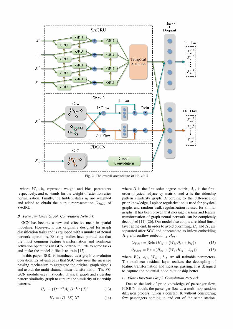
Fig. 2. The overall architecture of PB-GRU

where Wu, bu represent weight and bias parametersrespectively, and at stands for the weight of attention afternormalization. Finally, the hidden states ut are weightedand added to obtain the output representation ORGU ofSAGRU.

B. Flow similarity Graph Convolution Network

GCN has become a new and effective mean in spatialmodeling. However, it was originally designed for graphclassification tasks and is equipped with a number of neuralnetwork operations. Existing studies have pointed out thatthe most common feature transformation and nonlinearactivation operations in GCN contribute little to some tasksand make the model difficult to train [12].

In this paper, SGC is introduced as a graph convolutionoperation. Its advantage is that SGC only uses the messagepassing mechanism to aggregate the original graph signalsand avoids the multi-channel linear transformation. The FS-GCN module uses first-order physical graph and ridershippattern similarity graph to capture the similarity of ridershippatterns.

HP =(D−1/2AijD

−1/2)Xt (13)

HS =(D−1S

)Xt (14)

where D is the first-order degree matrix, Aij is the first-order physical adjacency matrix, and S is the ridershippattern similarity graph. According to the difference ofprior knowledge, Laplace regularization is used for physicalgraphs and random walk regularization is used for similargraphs. It has been proven that message passing and featuretransformation of graph neural network can be completelydecoupled [11],[26]. Our model also adopts a residual linearlayer at the end. In order to avoid overfitting, Hp and Hs areseparated after SGC and concatenate as inflow embeddingHif and outflow embedding Hof .

OFSif = Relu (Hif + (WifHif + bif )) (15)

OFSof = Relu (Hof + (WofHif + bof )) (16)

where Wif , bif , Wif , bif are all trainable parameters.The nonlinear residual layer realizes the decoupling offeature transformation and message passing. It is designedto capture the potential node relationship better.

C. Flow Direction Graph Convolution Network

Due to the lack of prior knowledge of passenger flow,FDGCN models the passenger flow as a multi-hop randomdiffusion process. Given a constant K without consideringfew passengers coming in and out of the same station,

the model assumes that the passengers are equally likelyto arrive at all stations within K hop, and builds a groupof K-hop flow direction graphs to aggregate fine-grainedhierarchical flow information.

h(K) =((

A(K) � C)D(K)−1

)Xif (17)

where A(k) represents the k-hop physical graph, C repre-sents the OD Flow Direction graph, D(k) represents theK-hop degree matrix, � represents the Hadamard product,and K is a hyper parameter. We denoted the this set ofgraph convolution results as hhid , which represents thepotential passenger flow between subway stations in k hop.

For a station in the metro system, the farther the station,the later the arrival time. The K-hop potential passengerflow can be regarded as time series, and due to the predictedtime interval, the beneficial flow for prediction should bea subset of hhid. Next, a causal convolution is applied tofurther extract the potential passenger flow, as shown inFig. 3 Before each convolution layer, zero padding wasapplied. Thus, the output has the same length as the input,and the network can only use the information of past timesteps. In addition, gate mechanism is also used in causalconvolution:

P = w1 ∗ hhid + b1 (18)

Q = w2 ∗ hhid + b2 (19)

hout = tanh (P + hhid)� sigmoid(Q) (20)

P and Q are the results of input hhid through differentconvolution kernels w1 and w2, parameters b1 and b2 arebias, and � represents Hadamard product. By stacking asmall number of causal convolution layers, the model canobtain the appropriate size of the receptive field to capturethe local continuous passenger flow. The final output isrepresented as OFDof after being cut.

Fig. 3. Causal Convolution

D. Output layer

Finally, the model uses two independent fully connectedlayers to fuse the embeddings in order to predict the futureinflow and outflow volumes respectively. It can obtain thepredicted value of T time steps at one time.

Y in = Win (OGRU‖OFSif ) + bin (21)

Y out = Wout (OGRU ‖OFSof‖OFDof ) + bout (22)

where Win, Wout, bin, bout represent the trainable weightand bias parameters, ‖ represents the concatenate operation,Y in and Y out are the inflow and outflow of all subwaystations respectively. Finally, Y in and Y out are stacked toY as the predicted output of our model.

V. EXPERIMENTS

A. Data sets

Two metro ridership benchmark datasets, HZMetro andSHMetro, are used to evaluate the performance of ourmethod. The details of these two datasets are summarizedin Table I. The training set, verification set, and test setare divided according to the proportion of the originalsource [7], and only Z-score normalization is used forpreprocessing.

B. Parameter Settings and Evaluation Metrics

Hyper-parameters: When training on HZMetro, thebatchsize is set to 48, the hidden state size of the GRU is650. As for SHMetro, batchsize and hidden state size are96 and 1,200 respectively. The ADAM optimizer is usedto minimize the L1 loss to train 350 epochs. The initiallearning rate is set at 10−3 and decays to 0.5 per 40 epochs.The regularization method is Dropout p = 0.4, for SAGRUand FDGCN, and p = 0.1 for others.

Evaluation Metrics: Average absolute error (MAE),mean absolute percentage error (MAPE) and root meansquare error (RMSE) are used to evaluate the performanceof different methods. The three indexes are defined asfollows:

MAE = 1N

N∑i=1

∣∣yi − yi∣∣ (23)

MAPE = 1N

N∑i=1

|yi−yi|yi (24)

RMSE = 1N

N∑i=1

|yi−yi|yi (25)

where yi represents the ground-truth , yi represents thepredicted value, and N represents the number of metrostation.

TABLE I: DATA SETS

Dataset HZMetro SHMetro

City HangZhou,China

ShangHai,China

Station 80 288

Physical Edge 248 958

Ridership/Day 2.35 million 8.82 million

Time Interval 15min 15min

Training Set 1/01/2019 –1/18/2019

7/01/2016 –8/31/2016

Validation Set 1/19/2019 –1/20/2019

9/01/2016 –9/09/2016

Testing Set 1/21/2019 –1/25/2019

9/10/2016 –9/30/2016

TABLE II. EXPERIMENTAL RESULTS ON HZMetro

Model15min 30min 60min

MAE MAPE RMSE MAE MAPE RMSE MAE MAPE RMSELSTM 23.43 14.41 40.13 24.38 15.54 42.33 26.74 19.88 47.90GCN 24.21 21.05 49.20 25.75 24.26 52.34 33.44 27.62 62.39

DCRNN 23.24 13.65 41.43 25.78 15.32 43.23 27.15 18.64 48.56STGCN 23.86 12.48 45.03 26.07 13.72 49.16 31.47 16.95 59.74

Graph-Wavenet 23.50 13.77 41.88 24.75 15.68 43.70 27.85 20.45 48.69PVGCN 22.20 13.15 38.12 23.13 13.87 40.00 24.55 16.35 42.26

GCN-SUBLSTM 22.22 13.16 39.83 22.84 13.76 41.08 24.58 15.73 44.48PB-GRU 22.13 13.30 36.55 22.90 13.75 38.33 23.91 14.87 40.02

TABLE III. EXPERIMENTAL RESULTS ON SHMETRO

Model15min 30min 60min

MAE MAPE RMSE MAE MAPE RMSE MAE MAPE RMSELSTM 23.50 20.23 47.08 24.50 22.64 49.63 26.87 26.16 56.53GCN 24.21 21.05 49.20 25.75 24.26 52.34 31.60 34.25 63.24

DCRNN 23.34 18.02 47.24 25.33 19.12 51.31 29.01 21.52 63.32STGCN 23.84 18.71 47.18 26.99 19.41 57.40 33.82 23.69 77.00

Graph-Wavenet 23.75 20.23 45.73 27.12 21.42 54.15 31.56 24.92 68.10PVGCN 22.85 16.95 45.47 24.16 18.83 50.18 26.37 19.67 58.49

GCN-SUBLSTM 22.75 16.50 46.09 23.77 17.62 49.04 25.87 20.21 55.41PB-GRU 22.70 15.98 43.35 23.74 16.52 46.46 25.72 17.90 51.80

TABLE IV. EXPERIMENTAL RESULTS OF FSGCN VARIANTS ON HZMETRO

Model15min 30min 60min

MAE MAPE RMSE MAE MAPE RMSE MAE MAPE RMSEBASE 23.19 13.86 38.43 23 .75 13.94 42.01 25.23 15.86 43.12

P-BASE 22.31 13.49 37.12 23.20 13.79 39.42 24.01 14.82 40.66D-BASE 22.45 13.58 37.41 23.23 13.82 39.05 24.17 14.83 40.96

PD-BASE 22.21 13.42 37.01 22.96 13.76 38.51 23.94 14.71 40.47

TABLE V. EXPERIMENTAL RESULTS OF FSGCN VARIANTS ON SHMETRO

Model15min 30min 60min

MAE MAPE RMSE MAE MAPE RMSE MAE MAPE RMSEBASE 23.46 16.25 45.78 24 .30 17.72 48.46 26.18 19.61 55.14

P-BASE 23.00 16.03 44.04 23.97 16.50 46.98 26.06 17.77 53.31D-BASE 23.02 16.03 44.21 24.07 16.51 47.36 26.25 17.70 54.17

PD-BASE 22.80 15.96 43.76 23.79 16.42 46.86 25.79 17.50 52.05

C. Compared Models

We compared our method with a variety of existingmodels including:

LSTM: Long-short term memory neural network, thispaper uses encoder - decoder structure to achieve predic-tion.

GCN: Graph convolution neural network, implementedaccording to [10].

DCRNN [4]: The diffusion convolutional recurrent neu-ral network uses the bidirectional random walk on the graphcombined with the encoder-decoder structure to learn thespatial-temporal dependence.

STGCN [5]: Spatial and Temporal Graph ConvolutionalNetwork, using Chebyshev Graph Convolution and GLU tocapture spatial-temporal dependence respectively.

Graph-Wavenet [6]: The method proposes an adaptivedependency matrix to capture hidden spatial correlationsand uses stacked causal convolution to process time series.

PVGCN [7]: The physical virtual graph convolutionalnetwork combines multi-graph convolution with GRU’sgating mechanism, and uses encode-decoder structure toachieve multi-step prediction.

GCN-SUBLSTM [9]: This model constructs a compos-ite graph, which uses double-layer multi-channel generalGCN to capture the spatial correlation of metro stations.

D. Performance Comparison

Performance of different models on HZMetro andSHMetro datasets are shown in Table II and Table III.For all the models, only LSTM and GCN capture a singletemporal or spatial correlation. The GCN model performsthe worst since it completely ignores the modeling ofthe time dimension. The LSTM achieves competitiveresults, but its MAPE is higher than the other models.This empirical evidence suggests that LSTM has poorfitting ability for medium and low passenger flow stations.STGCN and Graph-Wavenet are both time convolutionmodel with Graph convolution, but MAE and RMSE onthe two data sets are inferior to LSTM. This indicatesthat the temporal convolution model is not suitable forshort sequences with long time intervals. Both PVGCNand GCN-SUBLSTM have relatively accuracy. PVGCNhas a better prediction result on HZMetro, while GCN-SUBLSTM has a greater advantage in the long-termprediction of RMSE index in SHMetro. However, thesetwo models did not use independent graph convolutionmethod to model different spatial-temporal correlationpatterns of subway passenger flow. Our PB-GRU achievesthe best accuracy in almost all indicators, especiallyin SHMetro with complex subway network and largepassenger flow, the prediction performance is better thanall other models. Experimental results show that RMSEof the model is significantly improved compared with thesuboptimal model. This proves that the model is moresensitive to the sudden changes of passenger volume andcan better predict the marginal values.

E. Ablation Study

In order to study the contribution of each componentin our method, we further conduct extensive experimentsby removing each individual component respectively. Inparticular, we tried the following structures and conductedperformance comparison.

Base: Only SAGRU was used for the prediction.P-Base: FSGCN with first-order physical graph and

SAGRU were used for prediction.D-Base: FSGCN with ridership pattern similarity graph

and SAGRU were used for prediction.PD-Base: Complete FSGCN and SAGRU were used for

co-prediction.

Fig. 4. Influence of hyper-parameter K on HZMetro

Fig. 5. Influence of hyper-parameter K on SHMetro

The results are shown in Table IV and Table V. Itcan be seen from the tables that FSGCN , which isconstructed based on the similarity of traffic patternsbetween stations, significantly reduces the prediction error.As the predicted time interval becomes longer, the RMSEof PD-Base grows more gently than that of Base, whichproves that FSGCN captures the similar patterns betweenmetro stations. When only a single similar graph is usedfor convolution, the accuracy of P-base is higher than D-base, especially on SHMetro. In capturing similar trafficpatterns, the first-order physical graph is stronger than thesimilar graph constructed by DTW, which means that thetraffic patterns of adjacent subway stations in big cities areclosely correlated. Finally, PD-Base obtained the result withlower error by integrating the embeddings from two kindsof graph convolution, which is competitive with PB-GRUto a certain extent.

Fig. 6. The optimal value of K for different prediction intervals

In order to explore the influence of different K-hophyper-parameter in FDGCN, Fig. 4 and Fig. 5 show MAEand RMSE values of different K values ranging from 1to 10 in 15min prediction task . In the table, RMSE andMAE start at a high value, then gradually decrease to aminimum value, and finally increase as K become larger.In the predicted time interval of 15min, the optimal K valueof Shanghai Metro and Hangzhou Metro was set to 4 and 5,respectively. Fig. 6 shows the best hyper-parameter setting

when the minimum error is obtained in different predictedinterval tasks. It is very consistent with the common sensethat the longer the interval is, the larger the travel range ofpassengers will be. It effectively proves that FDGCN canimprove the prediction accuracy by modeling the inflowof the metro station within the K-hop. However, it alsoshould be noted that the inappropriate K value has a certainnegative impact on the prediction. Due to the differencesbetween subway and urban planning, how to determinethe value of K in different metro systems remain an openproblem.

Finally, the training time of different methods is furthercompared on the same workstation. Table VI shows thetime required to train an epoch for each method. Specif-ically, PVGCN and GCN-SUBLSTM, which are recentlyproposed for passenger volume prediction, are engagedin the comparison. We can see that PVGCN requires thelongest time to train. This is because the computationsof GRU cannot be paralleled, PVGCN integrates graphconvolution into GRU’s gating mechanism, and three graphconvolution operations are performed for each forwardpropagation. PB-GRU and GCN-SUBLSTM require similartraining time. It is worthy pointing out that our model hasless training time. It is due to the fact that both FSGCNand FDGCN use SGC as graph convolution, which reducesa large number of parameters compared with the traditionalGCN. In order to prove the efficiency of temporal attention,the additional training time of SAGRU was provided in thetable. The attention in the model could be regarded as a gatemechanism with temporal complexity O(n), so increasingthe size of training set will not lead to the exponential levelincrease of training time.

TABLE VI. COMPARISON OF TRAINING TIME PEREPOCH

Model HZMetro SHMetro

PVGCN 190.13s 345.64s

SAGRU 1.05s 1.78s

GCN-SUBLSTM 1.44s 2.83s

PB-GRU 1.27s 2.19s

F. VisualizationWe visualized the prediction results of SHMetro to

better demonstrate the model performance. Three instancesare selected to illustrate the performance of PB-GRU ondifferent passenger volumes. As shown in Fig. 7, PB-GRU is accurate in fitting both the overall trend andthe peaks. With the help of FDGCN, the model is lesslikely to underestimate the out flow peak. This is animportant reason why our model is lower than PVGCNand GCN-SUBLSTM on RMSE. Besides, we found thatthe periodicity of passenger flow in some subway stations(e.g. #166 station) is quite different. These special stationsare major source of prediction error. However, thanks toFSGCN and FDGCN, our method is able to handle suchcases according to the visualization of station #166.

VI. CONCLUSION AND FUTURE WORKS

In this paper, a deep learning model PB-GRU is proposedfor metro passenger volume prediction. In the model, We

design two completely different graph convolution modulesto capture flow pattern similarity and OD flow directionrespectively. Based on the experiments on two real-worlddatasets, the proposed PB-GRU is superior to the existingmodels in terms of precision and training efficiency. Moreablation studies further verify the effectiveness of the twograph convolution modules. In the future, we would furtherconsider the variation of the passenger flow pattern withinthe daily period and the functions of different stations, soas to achieve more accurate prediction in specific city area.

REFERENCES

[1] C. Ding, D. Wang, X. Ma, and H. Li, ”Predicting short-termsubway ridership and prioritizing its influential factors using gradientboosting decision trees,” Sustainability, vol. 8, pp. 1100, 2016.

[2] W. Jiang and J. Luo, ”Graph Neural Network for Traffic Forecasting:A Survey,” arXiv preprint arXiv:2101.11174, 2021.

[3] L. Zhao, Y. Song, C. Zhang, Y. Liu, P. Wang, T. Lin, et al., ”T-gcn: A temporal graph convolutional network for traffic prediction,”IEEE Transactions on Intelligent Transportation Systems, vol. 21,pp. 3848-3858, 2019.

[4] Y. Li, R. Yu, C. Shahabi, and Y. Liu, ”Diffusion ConvolutionalRecurrent Neural Network: Data-Driven Traffic Forecasting,” inInternational Conference on Learning Representations, 2018.

[5] B. Yu, H. Yin, and Z. Zhu, ”Spatio-temporal graph convolutionalnetworks: a deep learning framework for traffic forecasting,” inProceedings of the 27th International Joint Conference on ArtificialIntelligence, 2018, pp. 3634-3640.

[6] Z. Wu, S. Pan, G. Long, J. Jiang, and C. Zhang, ”Graph WaveNetfor deep spatial-temporal graph modeling,” in International JointConference on Artificial Intelligence 2019, 2019, pp. 1907-1913.

[7] L. Liu, J. Chen, H. Wu, J. Zhen, G. Li, and L. Lin,”Physical-Virtual Collaboration Modeling for Intra-and Inter-StationMetro Ridership Prediction,” IEEE Transactions on IntelligentTransportation Systems, 2020.

[8] X. Ma, J. Zhang, B. Du, C. Ding, and L. Sun, ”Parallel architectureof convolutional bi-directional LSTM neural networks for network-wide metro ridership prediction,” IEEE Transactions on IntelligentTransportation Systems, vol. 20, pp. 2278-2288, 2018.

[9] P. Chen, X. Fu, and X. Wang, ”A Graph ConvolutionalStacked Bidirectional Unidirectional-LSTM Neural Network forMetro Ridership Prediction,” IEEE Transactions on IntelligentTransportation Systems, 2021.

[10] T. N. Kipf and M. Welling, ”Semi-supervised classification withgraph convolutional networks,” arXiv preprint arXiv:1609.02907,2016.

[11] F. Wu, A. Souza, T. Zhang, C. Fifty, T. Yu, and K. Weinberger, ”Sim-plifying graph convolutional networks,” in International conferenceon machine learning, 2019, pp. 6861-6871.

[12] X. He, K. Deng, X. Wang, Y. Li, Y. Zhang, and M. Wang,”Lightgcn: Simplifying and powering graph convolution network forrecommendation,” in Proceedings of the 43rd International ACMSIGIR Conference on Research and Development in InformationRetrieval, 2020, pp. 639-648.

[13] Z. Cui, R. Ke, Z. Pu, and Y. Wang, ”Deep bidirectional andunidirectional LSTM recurrent neural network for network-widetraffic speed prediction,” arXiv preprint arXiv:1801.02143, 2018.

[14] J. Ye, J. Zhao, K. Ye, and C. Xu, ”How to build a graph-based deeplearning architecture in traffic domain: A survey,” IEEE Transactionson Intelligent Transportation Systems, 2020.

[15] W. Jiang and J. Luo, ”Big Data for Traffic Estimation and Prediction:A Survey of Data and Tools,” arXiv preprint arXiv:2103.11824,2021.

[16] T. Rakthanmanon, B. Campana, A. Mueen, G. Batista, B. Westover,Q. Zhu, et al., ”Searching and mining trillions of time seriessubsequences under dynamic time warping,” in Proceedings ofthe 18th ACM SIGKDD international conference on Knowledgediscovery and data mining, 2012, pp. 262-270.

[17] A. Miglani and N. Kumar, ”Deep learning models for trafficflow prediction in autonomous vehicles: A review, solutions, andchallenges,” Vehicular Communications, vol. 20, p. 100184, 2019.

[18] H. Yao, F. Wu, J. Ke, X. Tang, Y. Jia, S. Lu, et al., ”Deep multi-viewspatial-temporal network for taxi demand prediction,” in Proceedingsof the AAAI Conference on Artificial Intelligence, 2018.

[19] I. Sutskever, O. Vinyals, and Q. V. Le, ”Sequence to sequencelearning with neural networks,” arXiv preprint arXiv:1409.3215,2014.

[20] Z. Cui, R. Ke, Z. Pu, and Y. Wang, ”Deep bidirectional andunidirectional LSTM recurrent neural network for network-widetraffic speed prediction,” arXiv preprint arXiv:1801.02143, 2018.

[21] J. Zhang, Y. Zheng, and D. Qi, ”Deep spatio-temporal residualnetworks for citywide crowd flows prediction,” in Proceedings ofthe AAAI Conference on Artificial Intelligence, 2017.

[22] X. Shi, Z. Chen, H. Wang, D.-Y. Yeung, W.-K. Wong, and W.-c.Woo, ”Convolutional LSTM network: A machine learning approachfor precipitation nowcasting,” Advances in neural informationprocessing systems, vol. 28, 2015.

[23] W. Chen, L. Chen, Y. Xie, W. Cao, Y. Gao, and X. Feng, ”Multi-Range Attentive Bicomponent Graph Convolutional Network forTraffic Forecasting,” Proceedings of the AAAI Conference onArtificial Intelligence, vol. 34, pp. 3529-3536, 2020.

[24] C. Zheng, X. Fan, C. Wang, and J. Qi, ”Gman: A graph multi-

attention network for traffic prediction,” in Proceedings of the AAAIConference on Artificial Intelligence, pp. 1234-1241, 2020,

[25] C. Song, Y. Lin, S. Guo, and H. Wan, ”Spatial-temporal synchronousgraph convolutional networks: A new framework for spatial-temporalnetwork data forecasting,” in Proceedings of the AAAI Conferenceon Artificial Intelligence, 2020, pp. 914-921.

[26] J. Klicpera, A. Bojchevski, and S. Gunnemann, ”Predict thenpropagate: Graph neural networks meet personalized pagerank,”arXiv preprint arXiv:1810.05997, 2018.

[27] M. Liu, H. Gao, and S. Ji, ”Towards deeper graph neural networks,”in Proceedings of the 26th ACM SIGKDD International Conferenceon Knowledge Discovery & Data Mining, 2020, pp. 338-348.

[28] H. Zhu and P. Koniusz, ”Simple spectral graph convolution,” inInternational Conference on Learning Representations, 2021.

[29] Z. Liu, H. Chen, R. Feng, S. Wu, S. Ji, B. Yang, et al., ”Deep DualConsecutive Network for Human Pose Estimation,” in Proceedingsof the IEEE/CVF Conference on Computer Vision and PatternRecognition, 2021, pp. 525-534.

Fig. 7. Snapshot of three prediction instances. Station #277 and #12 are the lowest and highest average passenger volume in SHMetrorespectively, Station #166 is a more general instance with a different passenger volume pattern.