parallel local graph clustering - samsi · pdf fileparallel local graph clustering kimon...

Parallel Local Graph ClusteringKimon Fountoulakis, joint work with J. Shun, X. Cheng, F. Roosta-Khorasani, M. Mahoney, D. Gleich

University of California Berkeley and Purdue University

Based onJ. Shun, F. Roosta-Khorasani, KF, M. Mahoney. Parallel local graph clustering, VLDB 2016.

KF, X. Cheng, J. Shun, F. Roosta-Khorasani, M. Mahoney. Exploiting optimization for local graph clustering, arXiv:1602.01886v1.

KF, D. Gleich, M. Mahoney. An optimization approach to locally-biased graph algorithms, arXiv:1607.04940.

Local graph clustering: motivation

Facebook social network: colour denotes class year

Data: Facebook John Hopkins, A. L. Traud, P. J. Mucha and M. A. Porter, Physica A, 391(16), 2012

Normalized cuts: finds 20% of the graph


Local graph clustering: finds 3% of the graph


Local graph clustering: finds 17% of the graph


Current algorithms and running time

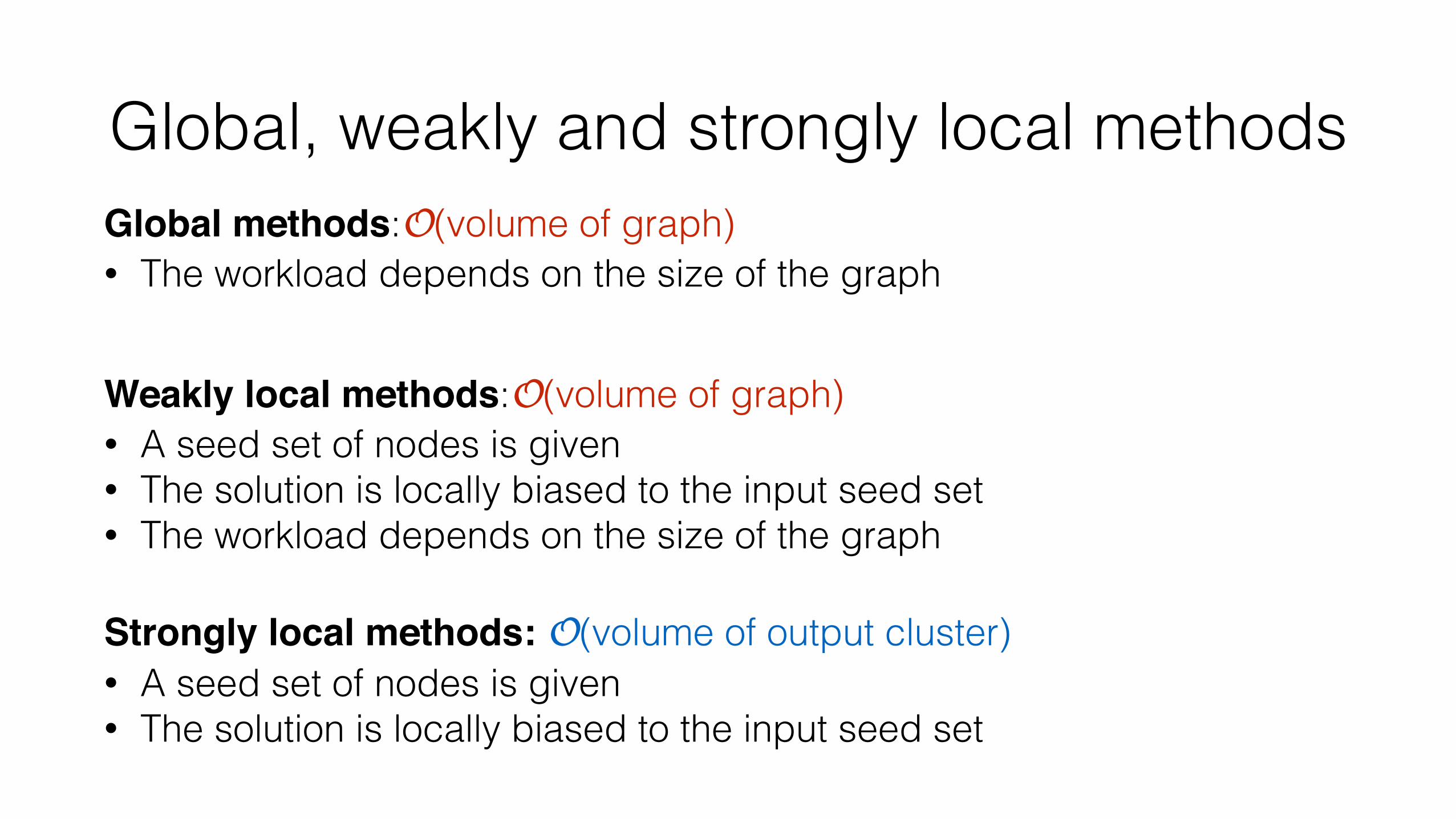
Global, weakly and strongly local methodsGlobal methods:O(volume of graph) • The workload depends on the size of the graph

Weakly local methods:O(volume of graph) • A seed set of nodes is given • The solution is locally biased to the input seed set • The workload depends on the size of the graph

Strongly local methods: O(volume of output cluster) • A seed set of nodes is given • The solution is locally biased to the input seed set

Global, weakly and strongly local methods

Global Weakly local Strongly local

Data: US Senate, P. Mucha, T. Richardson, K. Macon, M. Porter and J. Onnela, Science, vol. 328, no. 5980, pp. 876-878, 2010

2008191418601789

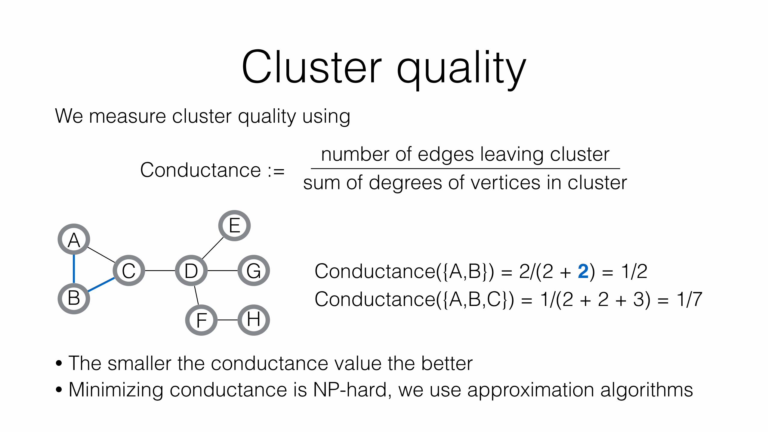
Cluster qualityWe measure cluster quality using

Conductance :=number of edges leaving cluster

sum of degrees of vertices in cluster

A

BC D

E

F

G

H

Conductance({A,B}) = 2/(2 + 2) = 1/2Conductance({A,B,C}) = 1/(2 + 2 + 3) = 1/7

• The smaller the conductance value the better • Minimizing conductance is NP-hard, we use approximation algorithms

Local graph clustering methods• MQI (strongly local): Lang and Rao, 2004 • Approximate Page Rank (strongly local): Andersen, Chung, Lang, 2006 • spectral MQI (strongly local): Chung, 2007 • Flow-Improve (weakly local): Andersen and Lang, 2008 • MOV (weakly local): Mahoney, Orecchia, Vishnoi, 2012 • Nibble (strongly local): Spielman and Teng, 2013 • Local Flow-Improve (strongly local): Orecchia, Zhu, 2014 • Deterministic HeatKernel PR (strongly local): Kloster, Gleich, 2014 • Randomized HeatKernel PR (strongly local): Chung, Simpson, 2015

• Sweep cut rounding algorithm

Shared memory parallel methodsthis talk

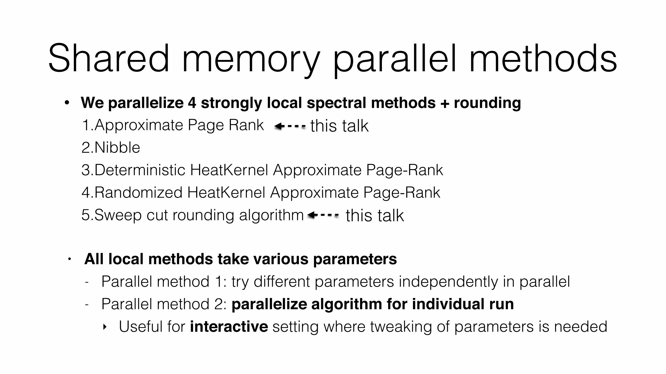
• We parallelize 4 strongly local spectral methods + rounding 1.Approximate Page Rank 2.Nibble 3.Deterministic HeatKernel Approximate Page-Rank 4.Randomized HeatKernel Approximate Page-Rank 5.Sweep cut rounding algorithm

• All local methods take various parameters- Parallel method 1: try different parameters independently in parallel - Parallel method 2: parallelize algorithm for individual run ‣ Useful for interactive setting where tweaking of parameters is needed

this talk

Approximate Page-Rank

Personalized Page-Rank vectorDegree matrix D

A B C D E F G HA 2

B 2

C 3

D 4

E 1

F 2

G 1

H 1

Pick a vertex u of interest and define a vector:

a teleportation parameter 0 ≤ α ≤ 1 and W = AD-1 then the PPR vector is given by solving:

((1� ↵)W + ↵seT )p = p , (I � (1� ↵)W )p = ↵s

A

BC D

E

F

G

H

Adjacency matrix AA B C D E F G H

A 1 1

B 1 1

C 1 1 1

D 1 1 1 1

E 1

F 1 1

G 1

H 1

s[u] = 1, s[v] = 0 8v 6= u

Approximate Personalized Page-RankR. Andersen, F. Chung and K. Lang. Local graph partitioning using Page-Rank, FOCS, 2006

Run a coordinate descent solver for PPR until: any vertex u satisfies r[u] ≥ -αρd[u]

• r is the residual vector, p is the solution vector • ρ>0 is tolerance parameter

Initialize: p = 0, r = -αsWhile termination criterion is not met do1. Choose any vertex u where r[u] < -αρd[u]2. p[u] = p[u] - r[u]3. For all neighbours v of u: r[v] = r[v] + (1-α)r[u]A[u,v]/d[u]4. r[u] = 0

{residual update

Final step: round the solution p using sweep cut.

Algorithm idea: iteratively spread probability mass from vector s around the graph.


Initialize: p = 0, r = -αs While termination criterion is not met do 1. Choose any vertex u where r[u] < -αρd[u] 2. p[u] = p[u] - r[u] 3. For all neighbours v of u: r[v] = r[v] + (1-α)r[u]A[u,v]/d[u] 4. r[u] = 0

A

B

C D

E

F

G

Hp=0, r=0

p=0, r=-α

p=0, r=0

p=0,r=0

p=0, r=0

p=0, r=0

p=0, r=0

p=0, r=0

krk1↵

= 1, kpk1 = 0,krk1↵

+ kpk1 = 1



A

B

C D

E

F

G

Hp=0, r=0

p=0.1, r=-α

p=0, r=0

p=0,r=0

p=0, r=0

p=0, r=0

p=0, r=0

p=0, r=0

krk1↵

= 1, kpk1 = 0.1,krk1↵

+ kpk1 = 1.1


Initialize: p = 0, r = -αs, where s is a probability vector While termination criterion is not met do 1. Choose any vertex u where r[u] < -αρd[u] 2. p[u] = p[u] - r[u] 3. For all neighbours v of u: r[v] = r[v] + (1-α)r[u]A[u,v]/d[u]4. r[u] = 0

A

B

C D

E

F

G

Hp=0, r=-0.45

p=0.1, r=0

p=0, r=-0.45

p=0,r=0

p=0, r=0

p=0, r=0

p=0, r=0

p=0, r=0

krk1↵

= 0.9, kpk1 = 0.1,krk1↵

+ kpk1 = 1.0



A

B

C D

E

F

G

Hp=0.045, r=0

p=0.1, r=-0.2025

p=0, r=-0.6525

p=0,r=0

p=0, r=0

p=0, r=0

p=0, r=0

p=0, r=0

krk1↵

= 0.855, kpk1 = 0.145,krk1↵

+ kpk1 = 1.0


Initialize: p = 0, r = -αs, where s is a probability vector While termination criterion is not met do 1. Choose any vertex u where r[u] < -αρd[u] 2. p[u] = p[u] - r[u] 3. For all neighbours v of u: r[v] = r[v] + (1-α)r[u]A[u,v]/d[u] 4. r[u] = 0

A

B

C D

E

F

G

Hp=0.045, r=-0.1957

p=0.1, r=-0.3982

p=0.0653, r=0

p=0,r=-0.1957

p=0, r=0

p=0, r=0

p=0, r=0

p=0, r=0

krk1↵

= 0.7897, kpk1 = 0.2103,krk1↵

+ kpk1 = 1.0

Running time APPR

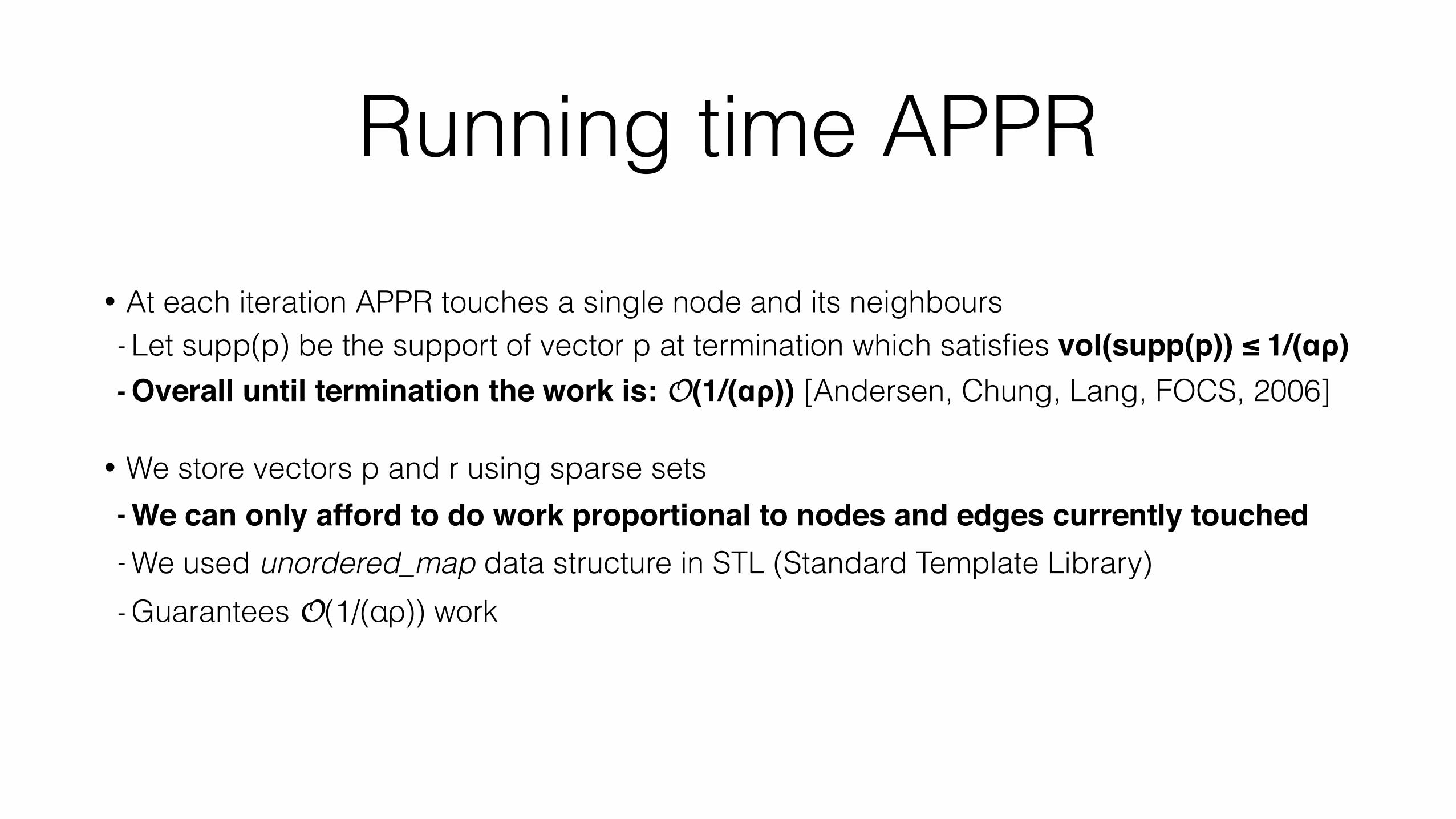
• At each iteration APPR touches a single node and its neighbours - Let supp(p) be the support of vector p at termination which satisfies vol(supp(p)) ≤ 1/(αρ) - Overall until termination the work is: O(1/(αρ)) [Andersen, Chung, Lang, FOCS, 2006]

• We store vectors p and r using sparse sets - We can only afford to do work proportional to nodes and edges currently touched- We used unordered_map data structure in STL (Standard Template Library) - Guarantees O(1/(αρ)) work

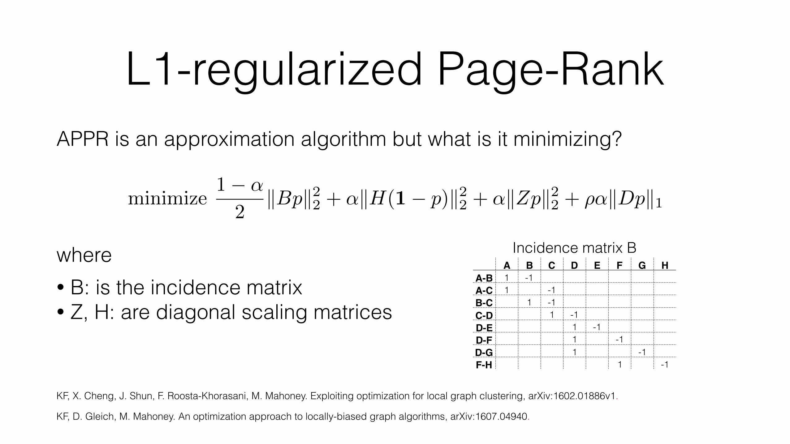
L1-regularized Page-RankAPPR is an approximation algorithm but what is it minimizing?

where• B: is the incidence matrix • Z, H: are diagonal scaling matrices

KF, X. Cheng, J. Shun, F. Roosta-Khorasani, M. Mahoney. Exploiting optimization for local graph clustering, arXiv:1602.01886v1.

KF, D. Gleich, M. Mahoney. An optimization approach to locally-biased graph algorithms, arXiv:1607.04940.

minimize1� ↵

2kBpk22 + ↵kH(1� p)k22 + ↵kZpk22 + ⇢↵kDpk1

Incidence matrix BA B C D E F G H

A-B 1 -1A-C 1 -1B-C 1 -1C-D 1 -1D-E 1 -1D-F 1 -1D-G 1 -1F-H 1 -1

Shared memory

Running time: work depth model

Model • Work: number of operations required • Depth: longest chain of sequential dependencies

Note that our results are not model dependent.

Let P be the number of cores available.

By Brent’s theorem [1] an algorithm with work W and depth D has overall running time: W/P + D.In practice W/P dominates. Thus parallel efficient algorithms require the same work as its sequential version.

Work depth model: J. Jaja. Introduction to parallel algorithms. Addison-Wesley Profesional, 1992

Brent’s theorem: [1] R. P. Brent. The parallel evaluation of general arithmetic expressions. J ACM (JACM), 21(2):201-206, 1974

Parallel Approximate Personalized Page-RankWhile termination criterion is not met do 1. Choose ALL (instead of any) vertex u where r[u] < -αρdeg[u] 2. p[u] = p[u] - r[u] 3. For all neighbours v of u: r[v] = r[v] + (1-α)/(2deg[u])r[u] 4. r[u] = (1-α)r[u]/2

• Asymptotic work remains the same: O(1/(αρ)). • Parallel randomized implementation: work O(1/(αρ)) and depth O(log(1/(αρ)).

- Keep track of two sparse copies of p and r - Concurrent hash table for sparse sets <— important for O(1/(αρ)) work - Use atomic increment to deal with conflicts - Use of Ligra (Shun and Blelloch 2013) to process only “active” vertices and their edges

• Same theoretical graph clustering guarantees, Fountoulakis et al. 2016.

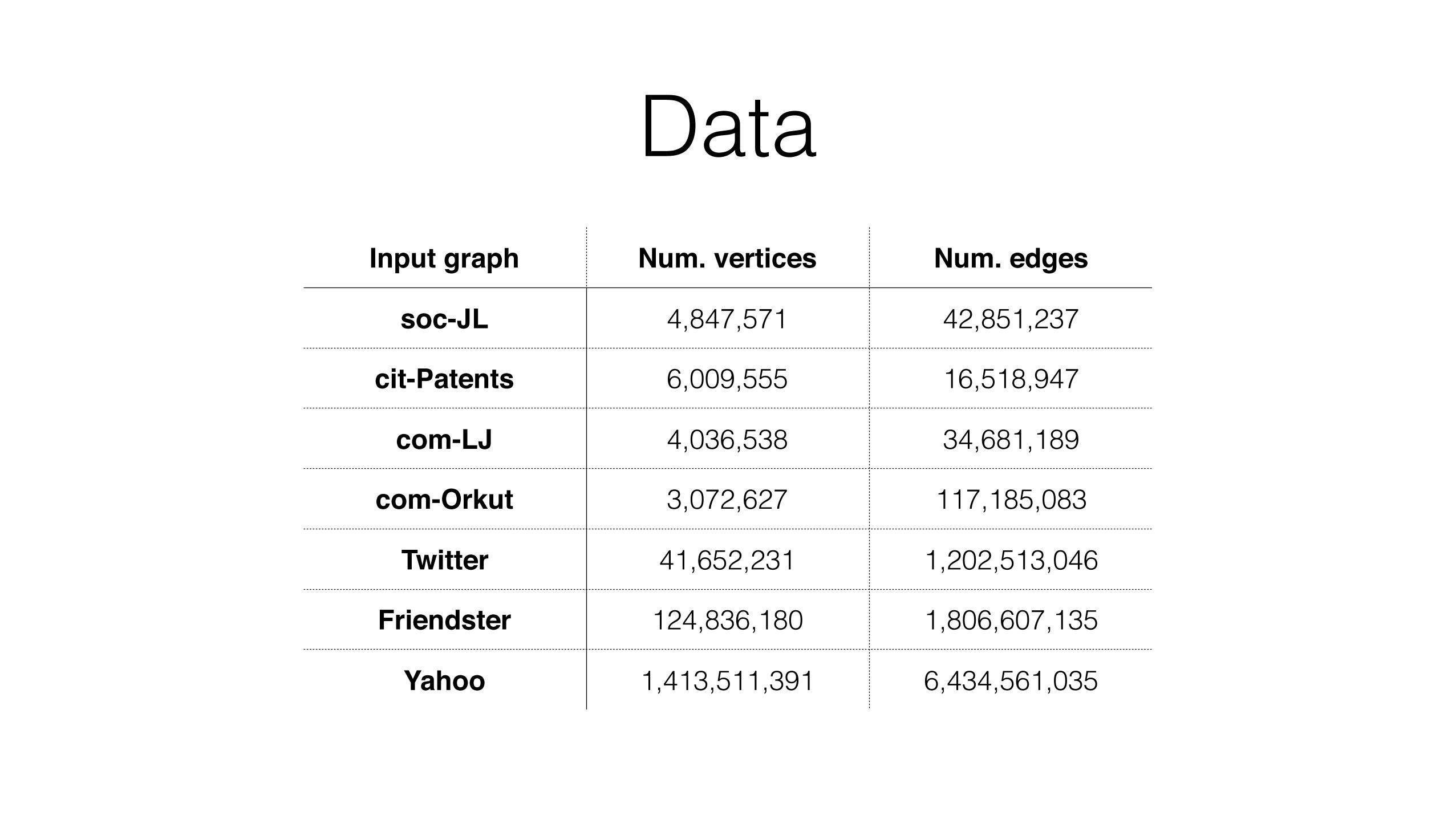
DataInput graph Num. vertices Num. edges

soc-JL 4,847,571 42,851,237

cit-Patents 6,009,555 16,518,947

com-LJ 4,036,538 34,681,189

com-Orkut 3,072,627 117,185,083

Twitter 41,652,231 1,202,513,046

Friendster 124,836,180 1,806,607,135

Yahoo 1,413,511,391 6,434,561,035

Performance

• Slightly more work for the parallel version • Number of iterations is significantly less

Performance

• 3-16x speed up • Speedup is limited by small active set in some iterations and memory effects

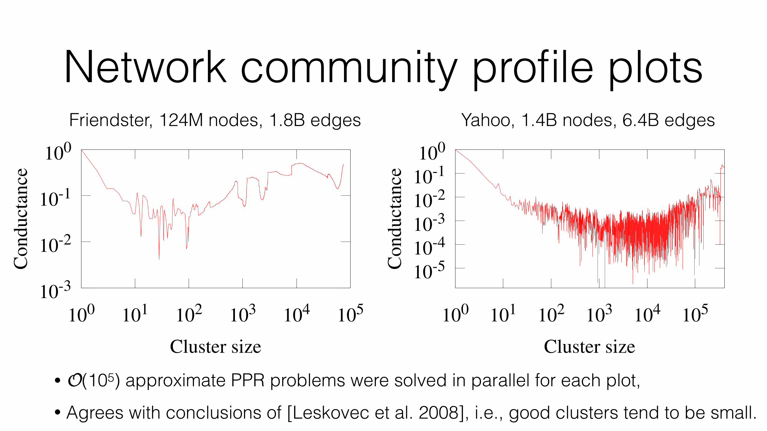
Network community profile plots

10-510-410-310-210-1100

100 101 102 103 104 105

Con

duct

ance

Cluster size

10

-3

10

-2

10

-1

10

0

10

0

10

1

10

2

10

3

10

4

10

5

Conductance

Cluster size

• O(105) approximate PPR problems were solved in parallel for each plot,

Friendster, 124M nodes, 1.8B edges Yahoo, 1.4B nodes, 6.4B edges

• Agrees with conclusions of [Leskovec et al. 2008], i.e., good clusters tend to be small.

Rounding: sweep cut• Round returned vector p of approximate PPR - 1st step (O(1/(αρ) log(1/(αρ))) work): Sort vertices by non-increasing value of non-zero p[u]/d[u]

- 2nd step (O(1/(αρ)) work): Look at all prefixes of sorted order and return the cluster with minimum conductance,

EA

B

C D G

F H2nd

1st 3rd 4thSorted vertices: {A,B,C,D}

Cluster Conductance{A} 1

{A,B} 1/2{A,B,C} 1/7

{A,B,C,D} 3/11

Parallel sweep cut• 1st step: Sort vertices by non-increasing value of non-zero p[u]/d[u].

- Use parallel sorting algorithm, O(1/(αρ) log(1/(αρ))) work and O(log(1/(αρ)) depth.

• 2nd step: Look at all prefixes of sorted order and return the cluster with minimum conductance. - Naive implementation: for each sorted prefix compute conductance, O((1/(αρ))2).

- We design a parallel algorithm based on integer sorting and prefix sums that takes O(1/(αρ)) time.

- The algorithm computes the conductance of ALL sets with a single pass over the nodes and the edges.

Parallel sweep cut: 2nd stepIncidence matrix B

A B C D E F G HA-B 1 -1

A-C 1 -1

B-C 1 -1

C-D 1 -1

D-E 1 -1

D-F 1 -1

D-G 1 -1

F-H 1 -1

Sorted vertices: {A,B,C,D}Cluster Sum cols B Volume Conductance

{A} 2 2 2/2=1

{A,B} 2 4 2/4=1/2{A,B,C} 1 7 1/7

{A,B,C,D} 3 11 3/11

EA

BC D G

F H

• Sort vertices - work: O(1/(αρ) log(1/(αρ))), depth: O(log(1/(αρ)))

• Represent matrix B with a sparse set using vertex identifiers and the order of vertices

- work: O(1/(αρ)), depth: O(log(1/(αρ))) • Use prefix sums to sum elements of the columns

- work: O(1/(αρ)), depth: O(log(1/(αρ)))

Parallel sweep cut: performance

1

10

100

1000

1 2 4 8 16 24 32 40

Running tim

e (secon

ds)

Number of cores

parallel sweep

sequential sweep

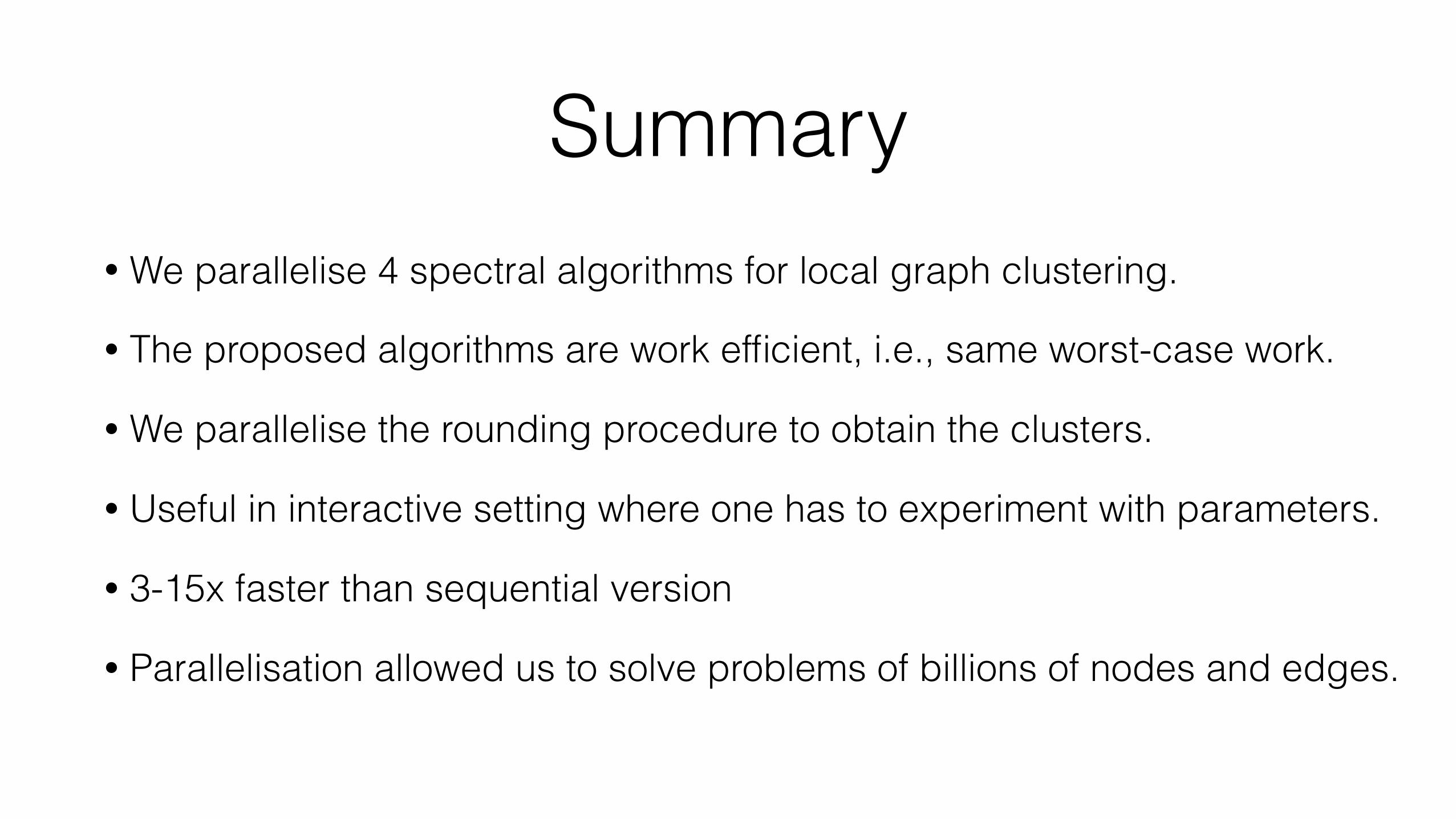
Summary• We parallelise 4 spectral algorithms for local graph clustering.

• The proposed algorithms are work efficient, i.e., same worst-case work.

• Useful in interactive setting where one has to experiment with parameters.

• 3-15x faster than sequential version

• Parallelisation allowed us to solve problems of billions of nodes and edges.

• We parallelise the rounding procedure to obtain the clusters.

Further work: distributed block coordinate descent

•Generalization to l2-regularized least-squares and kernel learning:

•Given a positive integer k - We reduce latency for BCD by a factor of k - at the expense of a factor of k more work and number of words.

A. Devarakonda, KF, J. Demmel, M. Mahoney: Avoiding communication in primal and dual block coordinate descent methods (work in progress ≤ month)

Thank you!

Collaboration network

Data: general relativity and quantum cosmology collaboration network, J. Leskovec, J. Kleinberg and C. Faloutsos, ACM TKDD, 1(1), 2007

Global graph clustering: normalized cuts


Local graph clustering: small clusters


Further work: distributed memory (work in progress)

Application: sample clusteringFeatures

Sample x1Sample x2

Sample x15

...

m x m Symmetric Adjacency matrix

Sample x6Sample x7Sample x8

Sample x11Sample x12

...

...

{Processor 1

{Processor 2

{Processor 3

distance(x1, x2)

m x n

Communication for approximate Page-Rank

While termination criterion is not met do 1. Choose any vertex u where r[u] < -αρdeg[u] 2. p[u] = p[u] - r[u] 3. For all neighbours v of u: 4. Compute A[v,u] = d(sample v, sample u) 5. r[v] = r[v] + (1-α)r[u]A[u,v]/deg[u] 6. r[u] = 0

Distribute m x 1 vectors p and r rp

P1

P1 P2

P2

P3

P3

Each processor has part of this set. Communication is needed to pick one node.

Communication for distance and residual.

Communication for approximate Page-Rank

MENTION CURRENT WORK BY DEMMEL

Loop unrolling for approximate Page-RankWhile termination criterion is not met do 1. Choose any vertex u where 2. 3.

where

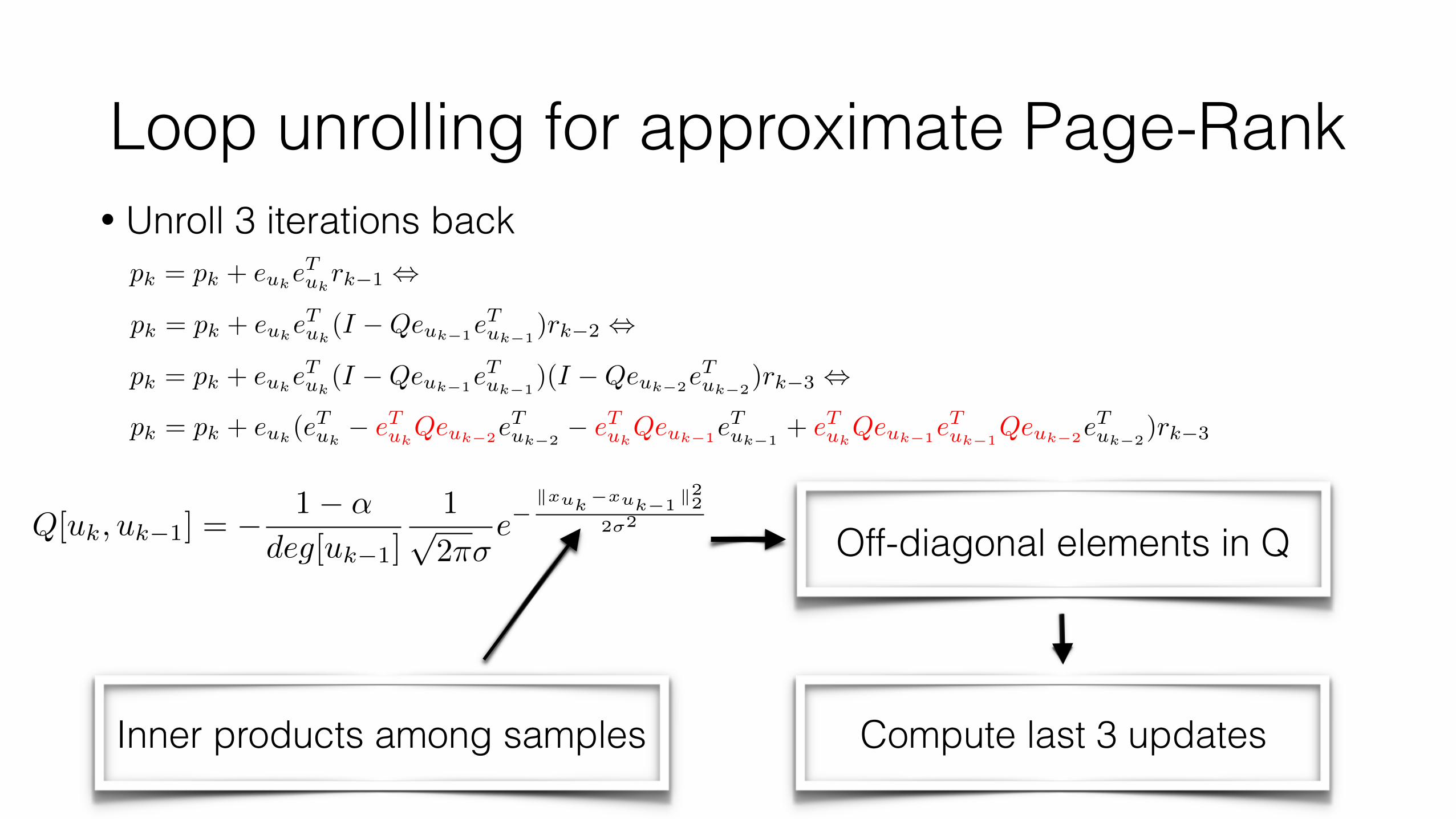
• Unroll 3 iterations back

pk = pk + eukeTuk(I �Qeuk�1e

Tuk�1

)rk�2 ,

pk = pk + eukeTukrk�1 ,


Tuk�1

)(I �Qeuk�2eTuk�2

)rk�3 ,

pk = pk + euk(eTuk

� eTukQeuk�2e

Tuk�2

� eTukQeuk�1e

Tuk�1

+ eTukQeuk�1e

Tuk�1

Qeuk�2eTuk�2

)rk�3

r[u] < �↵⇢deg[u]

p = p� eueTu r

r = (I �QeueTu )r

Q = I � (1� ↵)W

Loop unrolling for approximate Page-Rank• Unroll 3 iterations back


Tuk�1

)rk�2 ,

pk = pk + eukeTukrk�1 ,


Tuk�1

)(I �Qeuk�2eTuk�2

)rk�3 ,

pk = pk + euk(eTuk

� eTukQeuk�2e

Tuk�2

� eTukQeuk�1e

Tuk�1

+ eTukQeuk�1e

Tuk�1

Qeuk�2eTuk�2

)rk�3

Compute last 3 updates

Off-diagonal elements in Q

Inner products among samples

Q[uk, uk�1] = � 1� ↵

deg[uk�1]

1p2⇡�

e�kx

u

k

�x

u

k�1k22

2�2

Distributed Approximate Page-Rank

While termination criterion is not met do 1. Select ALL vertices from r[u] < -αρdeg[u] 2. In parallel: compute ALL x ALL Gram matrix 3. In parallel:

- for i=1,…,ALL, update vectors r and p using the Gram matrix

Input parameter s: number of vertices to update in parallel

Two communication events every s updates

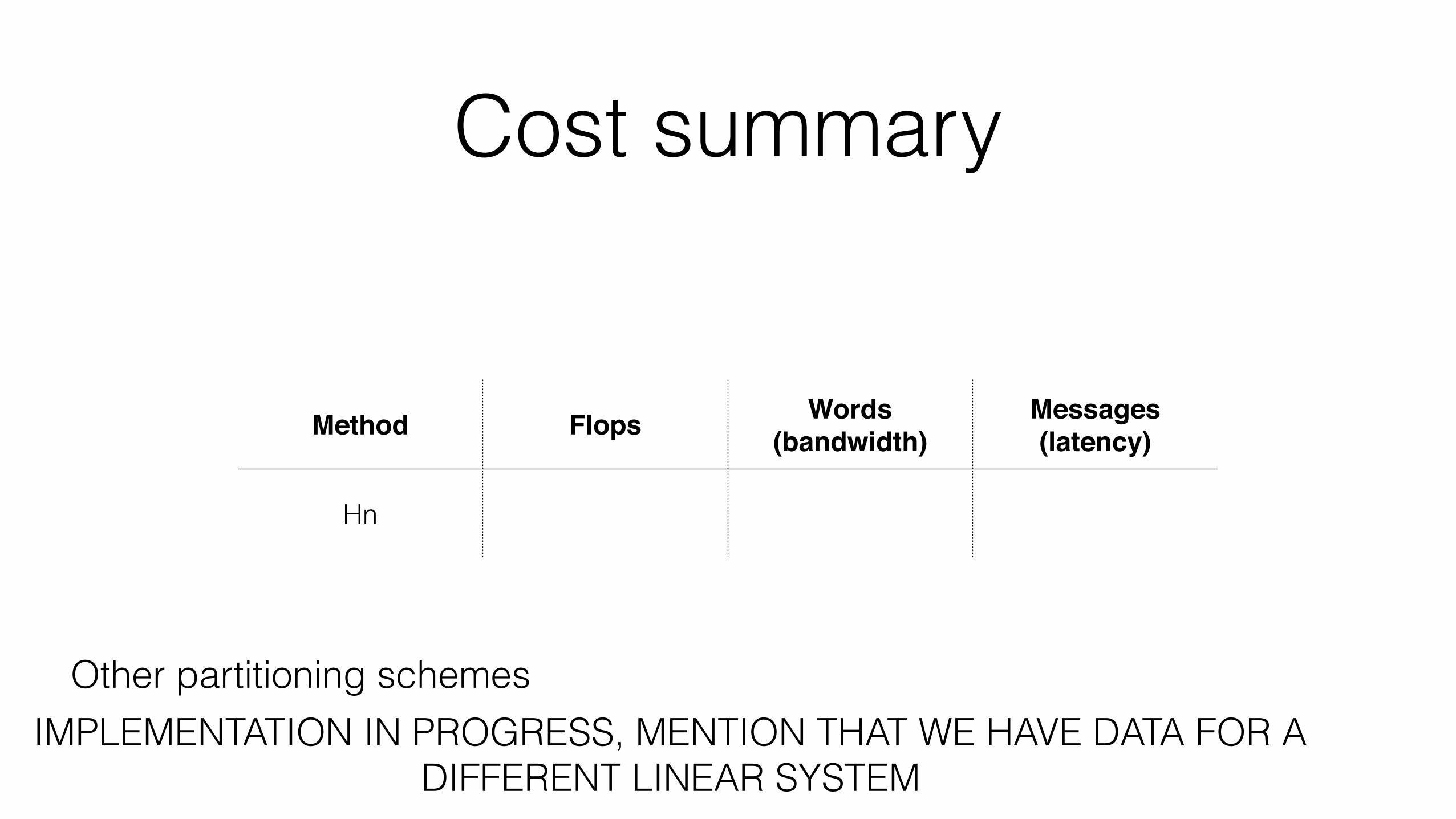
Cost summary

Method Flops Words (bandwidth)

Messages (latency)

Hn

IMPLEMENTATION IN PROGRESS, MENTION THAT WE HAVE DATA FOR A DIFFERENT LINEAR SYSTEM

Other partitioning schemes

parallel local graph clustering - samsi · pdf fileparallel local graph clustering kimon...

Documents