Parallel and Distributed Algorithms

Spring 2007

Johnnie W. Baker

The PRAM Model

for

Parallel Computation

References• Selim Akl, Parallel Computation: Models and Methods, Prentice

Hall, 1997, Updated online version available through website.• Selim Akl, The Design of Efficient Parallel Algorithms, Chapter 2

in “Handbook on Parallel and Distributed Processing” edited by J. Blazewicz, K. Ecker, B. Plateau, and D. Trystram, Springer Verlag, 2000.

• Selim Akl, Design & Analysis of Parallel Algorithms, Prentice Hall, 1989.

• Cormen, Leisterson, and Rivest, Introduction to Algorithms, 1st edition (i.e., older), 1990, McGraw Hill and MIT Press, Chapter 30 on parallel algorithms.

• Phillip Gibbons, Asynchronous PRAM Algorithms, Ch 22 in Synthesis of Parallel Algorithms, edited by John Reif, Morgan Kaufmann Publishers, 1993.

• Joseph JaJa, An Introduction to Parallel Algorithms, Addison Wesley, 1992.

• Michael Quinn, Parallel Computing: Theory and Practice, McGraw Hill, 1994

• Michael Quinn, Designing Efficient Algorithms for Parallel Computers, McGraw Hill, 1987.

Outline

• Computational Models• Definition and Properties of the PRAM Model• Parallel Prefix Computation• The Array Packing Problem• Cole’s Merge Sort for PRAM• PRAM Convex Hull algorithm using divide &

conquer • Issues regarding implementation of PRAM

model

Models in General

• An abstract description of a real world entity• Attempts to capture the essential features while

suppressing the less important details.• Important to have a model that is both precise

and as simple as possible to support theoretical studies of the entity modeled.

• If experiments or theoretical studies show the model does not capture some important aspects of the physical entity, then the model should be refined.

• Some people will not accept an abstract model of reality, but instead insist on reality.

• Sometimes reject a model if it does not capture every detail of the physical entity.

Parallel Models of Computation

• Describes a class of parallel computers• Allows algorithms to be written for a

general model rather than for a specific computer.

• Allows the advantages and disadvantages of various models to be studied and compared.

• Important, since the life-time of specific computers is quite short (e.g., 10 years).

Controversy over Parallel Models• Some professionals (usually engineers) will not

accept a parallel model unless it can currently be built.– Restricts the value of using models to explore and compare

potential future computers

• Engineers sometimes insist that a model must remain valid for unlimited number of processors – Parallel computers with more processors than the number

of atoms in the observable universe are unlikely to ever be built

– The models needed for vastly different numbers of processors may need to be different

• e.g., a few million or less vs 100 million or more.

The PRAM Model

• PRAM is an acronym for

Parallel Random Access Machine

• The earliest and best-known model for parallel computing.

• A natural extension of the RAM sequential model

• More algorithms designed for PRAM than probably all of the other models combined.

The RAM Sequential Model

• RAM is an acronym for Random Access Machine• RAM consists of

– A memory with M locations. • Size of M is as large as needed.

– A processor operating under the control of a sequential program which can

• load data from memory• store date into memory• execute arithmetic & logical computations on data.

– A memory access unit (MAU) that creates a path from the processor to an arbitrary memory location.

RAM Sequential Algorithm Steps

• A READ phase in which the processor reads datum from a memory location and copies it into a register.

• A COMPUTE phase in which a processor performs a basic operation on data from one or two of its registers.

• A WRITE phase in which the processor copies the contents of an internal register into a memory location.

PRAM Model Description• Let P1, P2 , ... , Pn be identical processors• Each processor is a RAM processor with a private local

memory.• The processors communicate using m shared (or global)

memory locations, U1, U2, ..., Um.

• Each Pi can read or write to each of the m shared memory locations.

• All processors operate synchronously (i.e. using same clock), but can execute a different sequence of instructions.– Akl book-chapter requires same sequence of instructions (SIMD)

• Each processor has a unique index called, the processor id, which can be referenced by the processor’s program.– Unstated assumption for most parallel models

PRAM Computation Step• Each PRAM step consists of three phases, executed in

the following order:– A read phase in which each processor may read a

value from shared memory– A compute phase in which each processor may

perform basic arithmetic/logical operations on their local data.

– A write phase where each processor may write a value to shared memory.

• Note that this prevents reads and writes from being simultaneous.

• Above requires a PRAM step to be sufficiently long to allow processors to do different arithmetic/logic operations simultaneously.

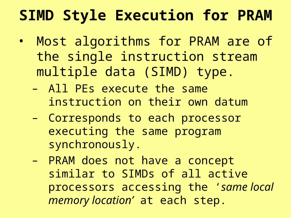
SIMD Style Execution for PRAM

• Most algorithms for PRAM are of the single instruction stream multiple data (SIMD) type.

– All PEs execute the same instruction on their own datum

– Corresponds to each processor executing the same program synchronously.

– PRAM does not have a concept similar to SIMDs of all active processors accessing the ‘same local memory location’ at each step.

SIMD Style Execution for PRAM(cont)

• PRAM model has been viewed by some as a shared memory SIMD. – Called a SM SIMD computer in [Akl 89]. – Called a SIMD-SM by early textbook [Quinn

87].– PRAM executions required to be SIMD [Quinn

94]– PRAM executions required to be SIMD in [Akl

2000]

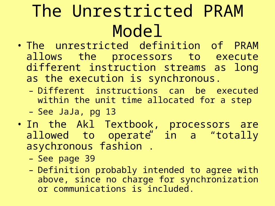
The Unrestricted PRAM Model• The unrestricted definition of PRAM allows the

processors to execute different instruction streams as long as the execution is synchronous. – Different instructions can be executed within the unit

time allocated for a step– See JaJa, pg 13

• In the Akl Textbook, processors are allowed to operate in a “totally asychronous fashion”.– See page 39– Definition probably intended to agree with above,

since no charge for synchronization or communications is included.

Asynchronous PRAM Models• While there are several asynchronous models, a typical

asynchronous model is described in [Gibbons 1993].• The asychronous PRAM models do not constrain

processors to operate in lock step.– Processors are allowed to run synchronously and

then charged for any needed synchronization.

• A non-unit charge for processor communication. – Take longer than local operations– Difficult to determine a “fair charge” when message-

passing is not handled in synchronous-type manner.• Instruction types in Gibbon’s model

– Global Read, Local operations, Global Write, Synchronization

• Asynchronous PRAM models are useful tools in study of actual cost of asynchronous computing

• The word ‘PRAM’ usually means ‘synchronous PRAM’

Some Strengths of PRAM Model

JaJa has identified several strengths designing parallel algorithms for the PRAM model.

• PRAM model removes algorithmic details concerning synchronization and communication, allowing designers to focus on problem features

• A PRAM algorithm includes an explicit understanding of the operations to be performed at each time unit and an explicit allocation of processors to jobs at each time unit.

• PRAM design paradigms have turned out to be robust and have been mapped efficiently onto many other parallel models and even network models.

PRAM Memory Access Methods • Exclusive Read (ER): Two or more processors

can not simultaneously read the same memory location.

• Concurrent Read (CR): Any number of processors can read the same memory location simultaneously.

• Exclusive Write (EW): Two or more processors can not write to the same memory location simultaneously.

• Concurrent Write (CW): Any number of processors can write to the same memory location simultaneously.

Variants for Concurrent Write

• Priority CW: The processor with the highest priority writes its value into a memory location.

• Common CW: Processors writing to a common memory location succeed only if they write the same value.

• Arbitrary CW: When more than one value is written to the same location, any one of these values (e.g., one with lowest processor ID) is stored in memory.

• Random CW: One of the processors is randomly selected write its value into memory.

Concurrent Write (cont)

• Combining CW: The values of all the processors trying to write to a memory location are combined into a single value and stored into the memory location. – Some possible functions for combining

numerical values are SUM, PRODUCT, MAXIMUM, MINIMUM.

– Some possible functions for combining boolean values are AND, INCLUSIVE-OR, EXCLUSIVE-OR, etc.

Additional PRAM comments1. PRAM encourages a focus on minimizing computation

and communication steps.• Means & cost of implementing the communications

on real machines ignored2. PRAM is often considered as unbuildable & impractical

due to difficulty of supporting parallel PRAM memory access requirements in constant time.

3. However, Selim Akl shows a complex but efficient MAU for all PRAM models (EREW, CRCW, etc) in that can be supported in hardware in O(lg n) time for n PEs and O(n) memory locations. (See [2. Ch.2].

4. Akl also shows that the sequential RAM model also requires O(lg m) hardware memory access time for m memory locations.

• Some strongly criticize cost in (4) but accept without question the cost in (3).

Parallel Prefix Computation• EREW PRAM Model is assumed for this

discussion• A binary operation on a set S is a function

:SS S.• Traditionally, the element (s1, s2) is denoted as

s1 s2.• The binary operations considered for prefix

computations will be assumed to be– associative: (s1 s2) s3 = s1 (s2 s3 )

• Examples– Numbers: addition, multiplication, max, min.– Strings: concatenation for strings– Logical Operations: and, or, xor

• Note: is not required to be commutative.

Prefix Operations

• Let s0, s1, ... , sn-1 be elements in S.

• The computation of p0, p1, ... ,pn-1 defined below is called prefix computation:

p0 = s0

p1 = s0 s1

.

.

.

pn-1 = s0 s1 ... sn-1

Prefix Computation Comments

• Suffix computation is similar, but proceeds from right to left.

• A binary operation is assumed to take constant time, unless stated otherwise.

• The number of steps to compute pn-1 has a lower bound of (n) since n-1 operations are required.

• Next visual diagram of algorithm for n=8 from Akl’s textbook. (See Fig. 4.1 on pg 153)– This algorithm is used in PRAM prefix algorithm– The same algorithm is used by Akl for the hypercube

(Ch 2) and a sorting combinational circuit (Ch 3).

EREW PRAM Prefix Algorithm

• Assume PRAM has n processors, P0, P1 , ... , Pn-1, and n is a power of 2.

• Initially, Pi stores xi in shared memory location si for i =

0,1, ... , n-1. • Algorithm Steps:

for j = 0 to (lg n) -1, do

for i = 2j to n-1 do

h = i - 2j

si = sh si

endfor

endfor

Prefix Algorithm Analysis

• Running time is t(n) = (lg n)

• Cost is c(n) = p(n) t(n) = (n lg n)

• Note not cost optimal, as RAM takes (n)

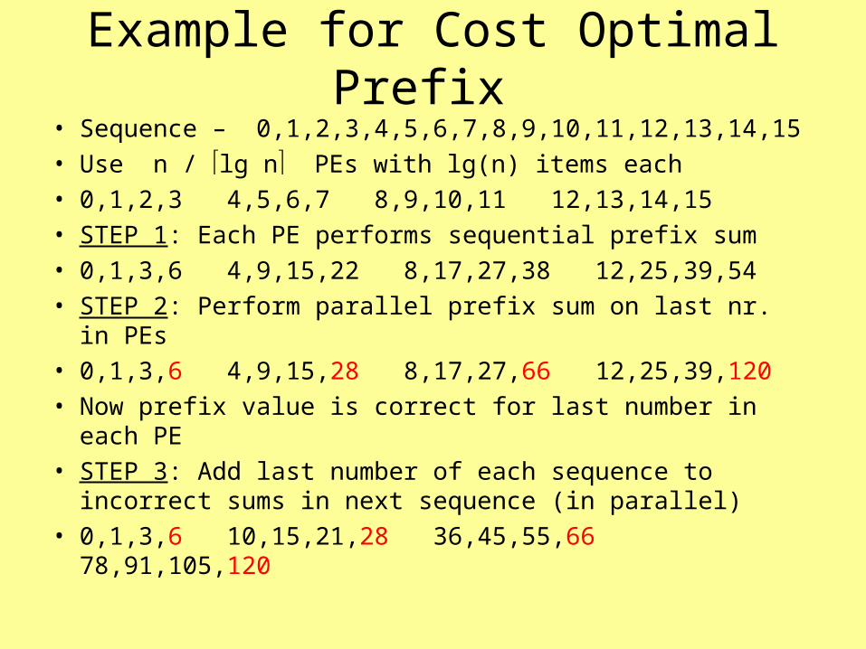
Example for Cost Optimal Prefix • Sequence – 0,1,2,3,4,5,6,7,8,9,10,11,12,13,14,15• Use n / lg n PEs with lg(n) items each• 0,1,2,3 4,5,6,7 8,9,10,11 12,13,14,15• STEP 1: Each PE performs sequential prefix sum• 0,1,3,6 4,9,15,22 8,17,27,38 12,25,39,54• STEP 2: Perform parallel prefix sum on last nr. in PEs• 0,1,3,6 4,9,15,28 8,17,27,66 12,25,39,120• Now prefix value is correct for last number in each PE• STEP 3: Add last number of each sequence to incorrect

sums in next sequence (in parallel)• 0,1,3,6 10,15,21,28 36,45,55,66 78,91,105,120

A Cost-Optimal EREW PRAM Prefix Algorithm

• In order to make the prefix algorithm optimal, we must reduce the cost by a factor of lg n.

• We reduce the nr of processors by a factor of lg n (and check later to confirm the running time doesn’t change).

• Let k = lg n and m = n/k• The input sequence X = (x0, x1, ..., xn-1) is partitioned into

m subsequences Y0, Y1 , ... ., Ym-1 with k items in each subsequence.– While Ym-1 may have fewer than k items, without loss

of generality (WLOG) we may assume that it has k items here.

• Then all sequences have the form,

Yi = (xi*k, xi*k+1, ..., xi*k+k-1)

PRAM Prefix Computation (X, ,S)

• Step 1: For 0 i < m, each processor Pi computes the prefix computation of the sequence Yi = (xi*k, xi*k+1, ...,

xi*k+k-1) using the RAM prefix algorithm (using ) and stores prefix results as sequence si*k, si*k+1, ... , si*k+k-1.

• Step 2: All m PEs execute the preceding PRAM prefix algorithm on the sequence (sk-1, s2k-1 , ... , sn-1) – Initially Pi holds si*k-1

– Afterwards Pi places the prefix sum sk-1 ... sik-1 in sik-1

• Step 3: Finally, all Pi for 1im-1 adjust their partial value sums for all but the final term in their partial sum subsequence by performing the computation

sik+j sik+j sik-1

for 0 j k-2.

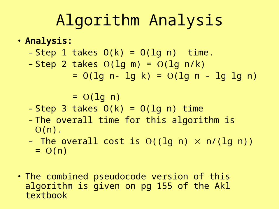
Algorithm Analysis• Analysis:

– Step 1 takes O(k) = O(lg n) time.– Step 2 takes (lg m) = (lg n/k)

= O(lg n- lg k) = (lg n - lg lg n) = (lg n)

– Step 3 takes O(k) = O(lg n) time – The overall time for this algorithm is (n).– The overall cost is ((lg n) n/(lg n)) = (n)

• The combined pseudocode version of this algorithm is given on pg 155 of the Akl textbook

The Array Packing Problem

• Assume that we have

– an array of n elements, X = {x1, x2, ... , xn}

– Some array elements are marked (or distinguished).• The requirements of this problem are to

– pack the marked elements in the front part of the array.

– place the remaining elements in the back of the array.

• While not a requirement, it is also desirable to– maintain the original order between the marked

elements– maintain the original order between the unmarked

elements

A Sequential Array Packing Algorithm

• Essentially “burn the candle at both ends”.• Use two pointers q (initially 1) and r (initially n).• Pointer q advances to the right until it hits an

unmarked element.• Next, r advances to the left until it hits a marked

element.• The elements at position q and r are switched

and the process continues.• This process terminates when q r.• This requires O(n) time, which is optimal. (why?)

Note: This algorithm does not maintain original order between elements

EREW PRAM Array Packing Algorithm

1.Set si in Pi to 1 if xi is marked and set si = 0 otherwise.

2. Perform a prefix sum on S =(s1, s2 ,..., sn) to obtain destination di = si for each marked xi .

3. All PEs set m = sn , the total nr of marked elements.

4. Pi sets si to 0 if xi is marked and otherwise sets si = 1.

5. Perform a prefix sum on S and set di = si + m for each unmarked xi .

6. Each Pi copies array element xi into address di in X.

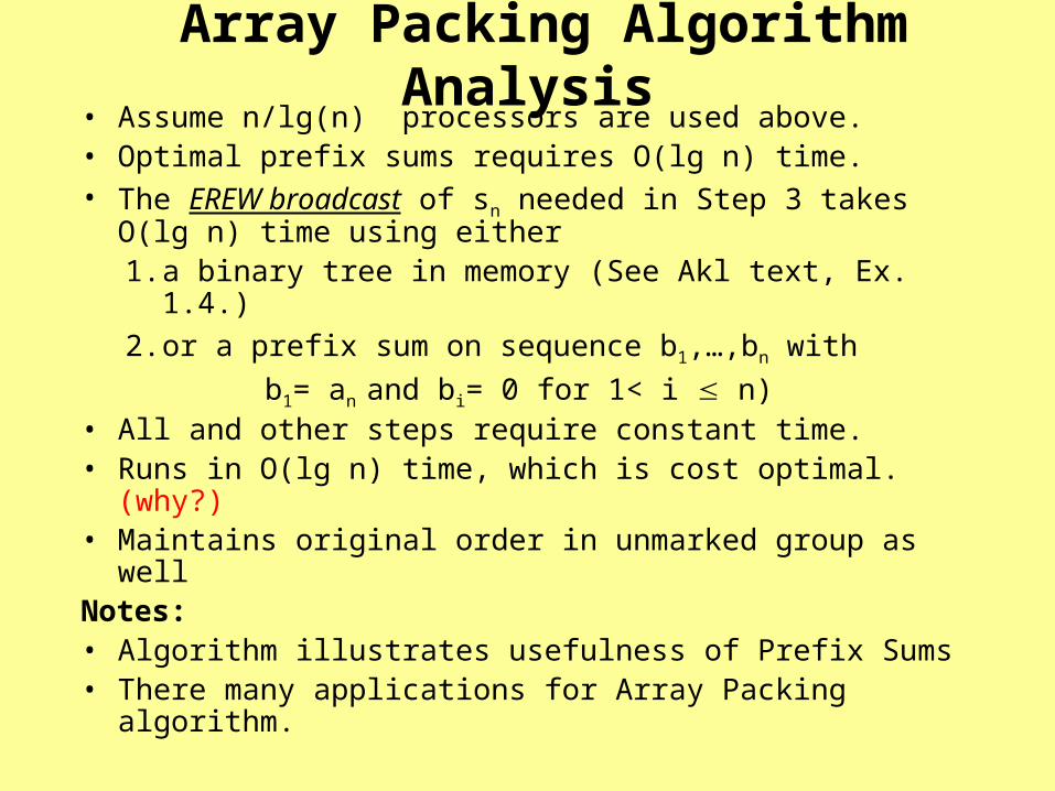
Array Packing Algorithm Analysis• Assume n/lg(n) processors are used above.• Optimal prefix sums requires O(lg n) time.• The EREW broadcast of sn needed in Step 3 takes

O(lg n) time using either1. a binary tree in memory (See Akl text, Ex. 1.4.)

2. or a prefix sum on sequence b1,…,bn with

b1= an and bi= 0 for 1< i n)• All and other steps require constant time.• Runs in O(lg n) time, which is cost optimal. (why?)• Maintains original order in unmarked group as wellNotes: • Algorithm illustrates usefulness of Prefix Sums• There many applications for Array Packing algorithm.

Cole’s Merge Sort for PRAM• Cole’s Merge Sort runs on EREW PRAM in O(lg n) using

O(n) processors, so it is cost optimal. – The Cole sort is significantly more efficient than most

other PRAM sorts.• Akl calls this sort “PRAM SORT” in book & chptr (pg 54)

– A high level presentation of EREW version is given in Ch. 4 of Akl’s online text and also in his book chapter

• A complete presentation for CREW PRAM is in JaJa.– JaJa states that the algorithm he presents can be

modified to run on EREW, but that the details are non-trivial.

• Currently, this sort is the best-known PRAM sort & is usually the one cited when a cost-optimal PRAM sort using O(n) PEs is needed.

References for Cole’s EREW Sort

Two references are listed below. • Richard Cole, Parallel Merge Sort, SIAM Journal

on Computing, Vol. 17, 1988, pp. 770-785.• Richard Cole, Parallel Merge Sort, Book-chapter

in “Synthesis of Parallel Algorithms”, Edited by John Reif, Morgan Kaufmann, 1993, pg.453-496

• Possible addition: May decide to add more on Cole sort from Akl’s text later, if time permits.

Comments on Sorting• A CREW PRAM algorithm that runs in

O((lg n) lg lg n) time and uses O(n) processors which is much simpler is given

in JaJa’s book (pg 158-160).– This algorithm is shown to be work optimal.

• Also, JaJa gives an O(lg n) time randomized sort for CREW PRAM on pages 465-473.– With high probability, this algorithm terminates in O(lg

n) time and requires O(n lg n) operations • i.e., with high-probability, this algorithm is work-

optimal.• Sorting is often called the “queen of the algorithms”:

• A speedup in the best-known sort for a parallel model usually results in a similar speedup other algorithms that use sorting.

Divide & Conquer Algorithms

• Three Fundamental Operations– Divide is the partitioning process– Conquer is the process of solving the base problem

(without further division)– Combine is the process of combining the solutions to

the subproblems

• Merge Sort Example– Divide repeatedly partitions the sequence into halves.– Conquer sorts the base set of one element– Combine does most of the work. It repeatedly merges

two sorted halves

• Quicksort Example – The divide stage does most of the work.

An Optimal CRCW PRAM Convex Hull Algorithm

• Let Q = {q1, q2, . . . , qn} be a set of points in the

Euclidean plane (i.e., E2-space).

• The convex hull of Q is denoted by CH(Q) and is the smallest convex polygon containing Q.– It is specified by listing its corner points (which are

from Q) in order (e.g., clockwise order).

• Usual Computational Geometry Assumptions:– No three points lie on the same straight line.– No two points have the same x or y coordinate.– There are at least 4 points, as CH(Q) = Q for n 3.

PRAM CONVEX HULL(n,Q, CH(Q))

1. Sort the points of Q by x-coordinate.

2. Partition Q into k =n subsets Q1,Q2,. . . ,Qk of k

points each such that a vertical line can separate Qi

from Qj

– Also, if i < j, then Qi is left of Qj.

3. For i = 1 to k , compute the convex hulls of Qi in

parallel, as follows:

– if |Qi| 3, then CH(Qi) = Qi

– else (using k=n PEs) call PRAM CONVEX HULL(k, Qi, CH(Qi))

4. Merge the convex hulls in {CH(Q1),CH(Q2), . . . ,CH(Qk)} into a convex hull for Q.

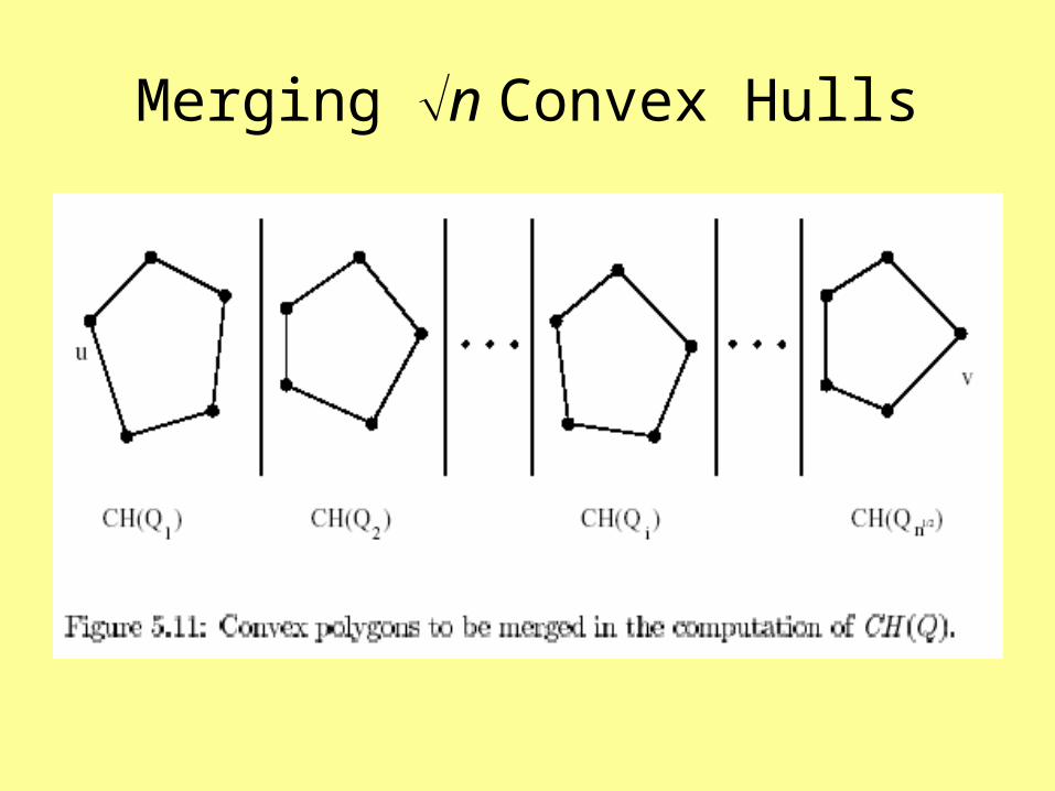
Merging n Convex Hulls

Details for Last Step of Algorithm

• The last step is somewhat tedious.• The upper hull is found first. Then, the lower hull

is found next using the same method.– Only finding the upper hull is described here– Upper & lower convex hull points merged into ordered

set

• Each CH(Qi) has n PEs assigned to it.• The PEs assigned to CH(Qi) (in parallel)

compute the upper tangent from CH(Qi) to another CH(Qj) . – A total of n-1 tangents are computed for each CH(Qi) – Details for computing the upper tangents will be

discussed separately

The Upper and Lower Hull

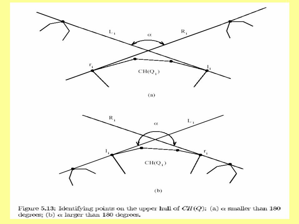
Last Step of Algorithm (cont)• Among the tangent lines to CH(Qi) and polygons to the

left of CH(Qi), let Li be the one with the smallest slope.– Use a MIN CW to a shared memory location

• Among the tangent lines to CH(Qi) and polygons to the right, let Ri be the one with the largest slope.– Use a MAX CW to a shared memory location

• If the angle between Li and Ri is less than 180 degrees, no point of CH(Qi) is in CH(Q).– See Figure 5.13 on next slide (from Akl’s Online text)

• Otherwise, all points in CH(Q) between where Li touches CH(Qi) and where Ri touches CH(Qi) are in CH(Q).

• Array Packing is used to combine all convex hull points of CH(Q) after they are identified.

Algorithm for Upper Tangents• Requires finding a straight line segment tangent

to CH(Qi) and CH(Qj), as given by line using a binary search technique– See Fig 5.14(a) on next slide

• Let s be the mid-point of the ordered sequence of corner points in CH(Qi) .

• Similarly, let w be the mid-point of the ordered sequence of convex hull points in CH(Qi).

• Two cases arise:– is the upper tangent of CH(Qi) and we are done.– Otherwise, on average one-half of the remaining

corner points of CH(Qi) and/or CH(Qj) can be removed from consideration.

• Preceding process is now repeated with the mid-points of two remaining sequences.

sw

sw

PRAM Convex Hull Complexity Analysis

• Step 1: The sort takes O(lg n) time.• Step 2: Partition of Q into subsets takes O(1) time.

– Here, Qi consist of points qk where k = (i-1)n +r for 1 i n

• Step 3: The recursive calculations of CH(Qi) for 1 i n in parallel takes t(n ) time (using n PEs for each Qi).

• Step 4: The big steps here require O(lgn) and are– Finding the upper tangent from CH(Qi) to CH(Qj) for

each i, j pair takes O(lgn ) = O(lg n)– Array packing used to form the ordered sequence of

upper convex hull points for Q.• Above steps find the upper convex hull. The lower

convex hull is found similarly.– Upper & lower hulls merged in O(1) time to ordered

set

Complexity Analysis (Cont)

• Cost for Step 3: Solving the recurrence relation

t(n) = t(n) + lg n

yields

t(n) = O(lg n)• Running time for PRAM Convex Hull is O(lg n)

since this is maximum cost for each step.• Then the cost for PRAM Convex Hull is

C(n) = O(n lg n).

Optimality of PRAM Convex Hull

Theorem: A lower bound for the number of sequential steps required to find the convex hull of a set of planar points is (n lg n)

• Let X = {x1, x2, . . . , xn } be any sequence of real numbers.

• Consider the set of planar points

Q = { (x1, x12) , (x2, x2

2) , . . . , (xn,xn2) .

• All points of Q lie on the curve y = x2, so all points of Q are in CH(Q).

• Apply any convex hull algorithm to Q.

Optimality of PRAM Convex Hull (cont)

• The convex hull returned is ‘sorted’ by the first coordinate, assuming the following rotation.– A sequence may require an around-the-end rotation

of items to get the least x-coordinate to occur first.– Identifying smallest term and rotating A takes only

linear (or O(n)) time.

• The process of sorting has a lower bound of n lg n basic steps.

• All of the above steps used to sort this sequence with the exception of finding the convex hull require only linear time.

• Consequently, a worst case lower bound for computing the convex hull is (n lgn) steps.

Overview of Implementation Issues for PRAM

References:• Chapter 2 of Akl’s Online Text• Akl’s Book-Chapter

Combinational Circuits

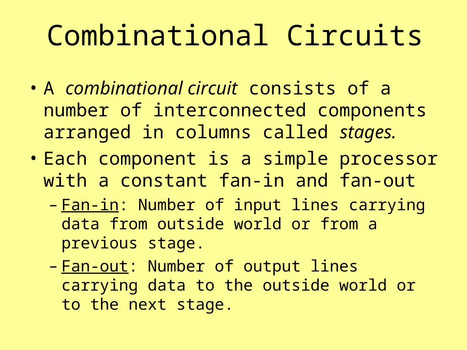
• A combinational circuit consists of a number of interconnected components arranged in columns called stages.

• Each component is a simple processor with a constant fan-in and fan-out– Fan-in: Number of input lines carrying data

from outside world or from a previous stage.– Fan-out: Number of output lines carrying data

to the outside world or to the next stage.

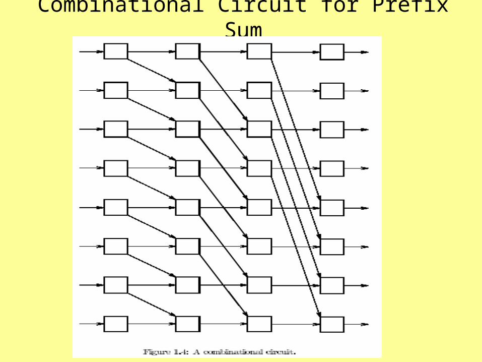
Combinational Circuit for Prefix Sum

Combinational Circuits (cont)• Component characteristics:

– Only active after input arrives– Computes a value to be output in O(1) time, usually

using only simple arithmetic or logic operations. – Component is hardwired to execute its computation.

• Component Circuit Characteristics– Has no program– Has no feedback

– Depth: The number of stages in a circuit

• Gives worst case running time for problem– Width: Maximal number of components per stage.– Size: The total number of components

• Note: size ≤ depth width

Two-way Combinational Circuits

• Sometimes used as a two-way devices• Input and output switch roles

– data travels from left-to-right at one time and from right-to-left at a later time.

• Useful particularly for communications devices.• Subsequently, the circuits are assumed to be

two-way devices. – Needed to support MAU (memory access unit) for

RAM and PRAM

Batcher’s Odd-Even Merging Circuit

• Diagram on next slide shows Batcher’s odd-even merging circuit– Has 8 inputs and 9 circuits. – Its depth is 3 and width is 4.– Merges two sorted list of input values of length 4

to produce one sorted list of length 8.

• Diagram is Figure 2.25 in Akl’s online text.

Batcher’s odd-even Merging Circuit

Batcher’s Odd-Even Merging Circuit(General Features)

• Input is two sequences of data.– Length of each is n/2.– Each sorted in non-decreasing order.

• Output is the combined values in sorted order.• Circuit has log n stages and at most n/2

components per stage.• The circuit size is O(n lg n)• Each component is a comparator:

– It receives 2 inputs and outputs the smaller of these on its top line and the larger on its bottom line.

– If switch set at each comparator to record its action, then circuit can later be used in “reverse” to return data to its origin.

Batcher’s Odd-Even Merging Circuit

• Diagram on next slide shows Batcher’s odd-even merging circuit– Has 8 inputs and 19 circuits. – Its depth is 6 and width is 4.– Merges two sorted list of input values of length 4

to produce one sorted list of length 8.

• Diagram is Figure 2.26 in Akl’s online text.

Batcher’s odd-even Sorting Circuit

Batcher’s Odd-Even Sorting Circuit

• Illustrated on preceding slide

• Input is sequence of n values.

• Output is the sorted sequence of these values.

• Has O(lg n) phases, each consisting of one or more odd-even merging circuits (stacked vertically & operating in parallel).– O(lg2 n) stages and at most n/2 processors

per stage.– Size is O(n lg2 n)

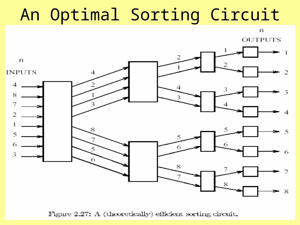
An Optimal Sorting Circuit

An Optimal Sorting Circuit• A complete binary tree with n leaves.

– Note: 1+ lg n levels and 2n-1 nodes

• Non-leaf nodes are circuits (of comparators).

• Each non-leaf node receives a set of m numbers

– Splits into m/2 smaller numbers sent to upper child circuit & remaining m/2 sent to the lower child circuit.

• Sorting Circuit Characteristics– Overall depth is O(lg n) and width is O(n).– Overall size is O(n lg n).

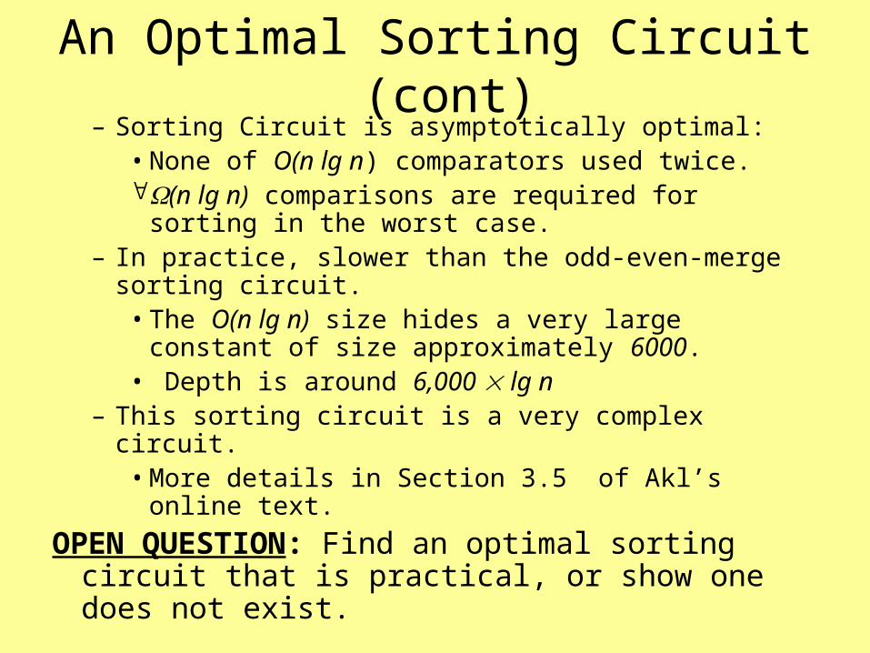
An Optimal Sorting Circuit (cont)– Sorting Circuit is asymptotically optimal:

• None of O(n lg n) comparators used twice.(n lg n) comparisons are required for sorting in

the worst case.– In practice, slower than the odd-even-merge sorting

circuit.• The O(n lg n) size hides a very large constant of

size approximately 6000.• Depth is around 6,000 lg n

– This sorting circuit is a very complex circuit. • More details in Section 3.5 of Akl’s online text.

OPEN QUESTION: Find an optimal sorting circuit that is practical, or show one does not exist.

A Memory Access Unit for RAM• A MAU for RAM is given by using a

combinational circuit.• See Chapter 2 of online text or book-chapter.• Implemented as a binary tree.• The PE is connected to the root of this tree and

each leaf is connected to a memory location.• If there are M memory locations for the PE then

– The access time (i.e., depth) is (lg M).– Circuit Width is (M)– Tree has 2M-1 = (M) switches– Size is (M).

• Assume tree links support 2-way communication• Using pipelining, this allows two or more data to

travel the same or opposite directions at the same time.

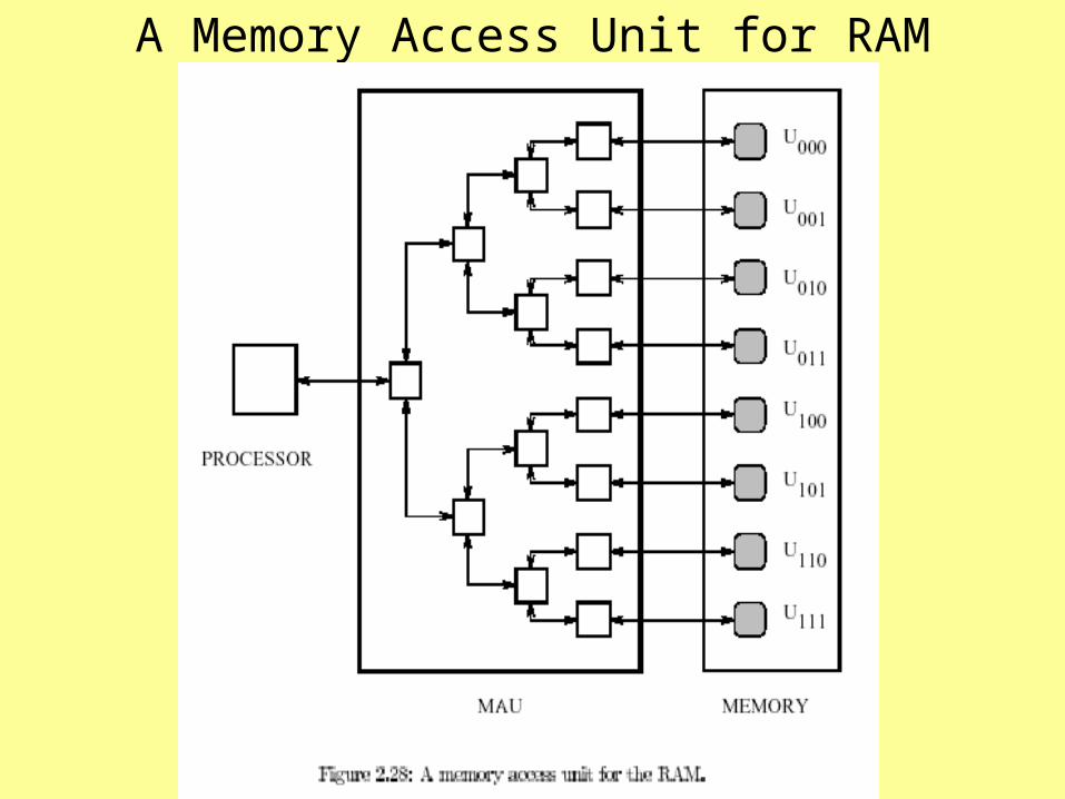
A Memory Access Unit for RAM

Optimality of Preceding RAM MAU

• The MAU will be implemented as a combinational circuit, so components must have a constant fan-out d.

• A Lower bound on circuit depth for a MAU.– M memory locations M output lines

(M) lower bound on circuit width.– At most ds-1 locations can be reached in s stages– In order for ds-1 M to be true, we must have

s-1 = logd(ds-1 ) logd (M)

– It follows that a lower bound on the MAU circuit depth for RAM is) (logd (M))

• Since (logd (M)) = (lg M), the preceding binary RAM MAU has optimal depth

A Comment on Optimality Proof

• No advantage is gained by allowing a non-constant fan-out– Basically the same argument applies using d =

maximum fan-out.

A Binary Tree MAU Implementation• Implemented as a binary tree of switches, as in

Fig 2.28.• Processor sends a location “a” to access

memory location Ua .• MAU decodes the address bit-by-bit.• For 1 i lg M, the switch at stage i examines

the ith most significant bit.• If 0, the switch sends “a” to top subtree;

otherwise “a” is sent to bottom subtree.– This creates a path from processor to Ua .

• If a value is to be written to Ua , this is handled by the leaf.

• If a processor wishes to read Ua , the leaf sends this value back to processor along same path.

RAM MAU Analysis Summary

• Depth and running time is (lg M).

• Width is (M)

• Tree has 2M-1 = (M) switches

• Size is (M).

A MAU for PRAM

• A memory access unit for PRAM is also given by Akl– Overview of how this MAU works discussed here– The MAU creates a path from each PE to each

memory location and handles all of the following: ER, EW, CR, CW.

• Handles all CW versions discussed (e.g., “combining”).

– Assume n PEs and M global memory locations.– We will assume that M is a constant multiple of n.

• Then M = (n).– A diagram for this MAU is given in Akl, Fig 2.30

Lower Bounds For PRAM MAU• Since there are M memory locations, M output lines

are required and (M) is a lower bound on the circuit width.

• By the same argument used for RAM, (lg M) is a lower bound on the circuit depth.

• A Lower Bound on circuit size for an arbitrary MAU for PRAM.– Let x be the number of switches used.– Let b be the maximum number of states (i.e.,

configurations) possible for these switches.• E.g., binary switches can direct data 2 ways.

– The entire circuit can have bx states.– Assume simplest memory access of EREW– With EREW, there are M! ways for M PEs to

access M memory locations (a worst case)

Lower Bounds For PRAM MAU (cont)

– Since the number of possible states for this circuit is bx, it follows that bx M!

– Since lg(M!) = (M lg M) by corollary to Sterling’s Formula (pg 35 of CLR reference),

x is (M logb M).

– This shows circuit size is (M lg M).• The preceding lower bound must hold for the

weakest access (i.e., EREW), so it must hold for all the other accesses as well.

PRAM MAU Memory Access Steps

• Diagram in Akl’s Figure 2.30 is assumed below.• Assume that the ith PE produces the record

(Instruction, ai, di, i) where “Instruction” is ER, CR, EW, etc. and

ai is the memory address

di is storage for read/write datum.• Each memory cell Uj produces a record

(Instruction, j, hj) where “Instruction” is initially empty.

j is the address of Uj

hj is the memory content of Uj .

PRAM MAU Memory Access Steps• The sorting circuit in diagram sorts processor

records using the memory address ai.– Ties broken by sorting on value of i.

• The values of j in second coordinate of memory records are already sorted.

• The two sorted sets are merged and sorted on their 2nd coordinate.– Two sets were already presorted on 2nd coordinate– In case of a tie, the processor record precedes the

memory record.

• Comparators must be slightly more complex.– Must handle information transfers– Must handle arithmetic & logic operations

Memory Access Steps (cont)• Additionally, comparators must have bit to store

straight/reverse routing information for use in reverse routing.

• All necessary information transfers between processor records and memory records occur at within comparators in the merging circuit.– Possible since each processor record with memory

address j is brought together in a comparator with the memory record with memory address j.

• Information transfers include– Instruction field transfer to memory record.– For ER, the memory value is transferred to processor

record (i.e., dihj) when these two records meet in a comparator.

– For EWs, value to be written is transferred to memory record (i.e., hj di) when these two records meet in a comparator.

CR Memory Access• The transfers for a CR is more complex.• Recall each memory record enter on top half of

the input to merge, but after merge it will immediately follow all PE records seeking to read its value.

• When a memory record meets a PE record seeking its value, the memory value is transferred to a processor record (i.e., d i hj)

• Since memory input is at top of merge but will move past all PE records seeking to read it, the record for each Pj seeking to read Ui will meet the Ui record in a comparator

CW Memory Access• The CW action (e.g., common, priority, AND,

OR, SUM) is also more complex.– Below description given for SUM. Others are

similar.– After the processor and memory records are

merged, the records of all processors wishing to write to the same memory location Uj are contiguous and precede the record for Uj .

– During the forward routing, the Uj record will have met a PE wishing to write to it, and will have its instruction value set (e.g., CW-ADD) an its hj value set to zero.

CW Memory Access Steps (cont)– During reverse routing, each of these PE records and

the Uj record trace out a binary tree that has memory location Uj as its root.

– It is important to observe that Uj meets each Pk that wishes to write to Uj once and only once on both incoming and reverse routing.

– When the record for a processor Pk writing to location i meets the record for Ui, the value recorded for Ui

(initially set to 0) becomes di+hk .

• The other Concurrent Writes are calculated similarly

– Will need an extra memory component in Ui in case of

PRIORITY Write to keep up with largest value.

Comparator size• Each needs to remember the line each record

arrived on initially to use for reverse routing. • This allows memory records to be shipped back

for a WRITE and processor records to be shipped back for a READ.

• A one bit per record in each comparator is sufficient for reverse routing.

• In case pipelining is used, comparators will need O(lg M) bits [since O(lg M) stages].

• Reasonable to provide O(lg M) bits for this, as registers are needed to handle values and addresses needed with a memory of size M.

Complexity Evaluation for Practical MAU

• Assume that MAU uses the odd-even merging and sorting circuits of Batcher – See Figs 2.25 and 2.26 (or examples 2.8

and 2.9) of Akl’s online textbook

• We assumed that M is (n).

• Since the sorting circuit has the larger complexity– MAU has width O(M) = O(n)– MAU has running time O(lg2M) = O(lg2n)– MAU has size O(M lg2M) = O(n lg2n)

A Theoretically Optimal MAU

• Next, assume that the sorting circuit used in MAU is the optimal sorting circuit

• Since we assume n is (M),

– MAU has width (M) = (n)

– MAU has depth or running time (lg M) = (n)

– MAU has size (M lg M) = (n lg n)

• These bounds match the previous lower bounds (up to a constant) and hence are optimal.

Additional Comments• Both implementations of this MAU can support

all of the PRAM models using only the same resources that are required to support the weakest EREW PRAM model.

• The first implementation using Batcher’s sort is practical while the second is not but is optimal.

• Note that EREW could be supported by the use of a MAU consisting of a binary tree for each PE that joins it to each memory location. – Not practical, since n binary trees are required and

each memory location must be connected to each of the n binary trees.