parallel adaptive mesh generation

Computing Systems in Engineering Vol. 2, No. 1, pp. 75 101, 1991 0956-0521/91 $3.00 ~- 0.00 Printed in Great Britain. ~t; 1991 Pergamon Press plc

PARALLEL ADAPTIVE MESH GENERATION

A. I. K H A N t and B. H. V. TOPPING +

tPostgraduate Research Student and :~Professor of Structural Engineering, Heriot-Watt University, Riccarton, Edinburgh, EHI4 4AS, U.K.

(Received 5 May 1991; revised 25 May 1991)

Abstract---Unstructured meshes have proved to be a powerful tool for adaptive remeshing of finite element idealizations. This paper presents a transputer-based parallel algorithm for two dimensional unstructured mesh generation. A conventional mesh generation algorithm for unstructured meshes is reviewed by the authors, and some program modules of sequential C source code are given. The concept of adaptivity in the finite element method is discussed to establish the connection between unstructured mesh generation and adaptive remeshing.

After these primary concepts of unstructured mesh generation and adaptivity have been presented, the scope of the paper is widened to include parallel processing for un-structured mesh generation. The hardware and software used is described and the parallel algorithms are discussed. The Parallel C environment for processor farming is described with reference to the mesh generation problem. The existence of inherent parallelism within the sequential algorithm is identified and a parallel scheme for unstructured mesh generation is formulated. The key parts of the source code for the parallel mesh generation algorithm are given and discussed. Numerical examples giving run times and the consequent "speed-ups" for the parallel code when executed on various numbers of transputers are given. Comparisons between sequential and parallel codes are also given. The "speed-ups" achieved when compared with the sequential code are significant. The "speed-ups" achieved when networking further transputers is not always sustained. It is demonstrated that the consequent "speed-up" depends on parameters relating to the size of the problem.

!. INTRODUCTION

Although the finite element formulation is a powerful tool in structural analysis its accurate use is dependent on human expertise. The solutions are always approximate and if a poor domain discretization is involved then the results may be dangerously different from the true solution.

Research on adaptivity and error estimation ~ aims at removing the human factor and automating the finite element procedure. For any adaptive finite element technique to be implemented, it is essential that a mesh generator is available to generate meshes in accordance with the information received from the adaptive calculations of the a posteriori error estimator 2 using the finite element solution. A limit on the overall error for the finite element problem is fixed and the procedure is repeated until a solution mesh is obtained with the error over the whole domain being within acceptable limits.

An algorithm based upon the advancing front technique of Peraire et al. 2 has been used in Refs 1, 2 and 3 for adaptive remeshing. Taking this mesh generation algorithm as a potent finite element pre- processor the object of the study has been to develop it for use in a parallel computing environment.

The unstructured mesh generator of Peraire et al. 4

relies upon efficient searching algorithms of Bonet and Peraire 5 for locating the points inside certain regions and determining intersections between geometrical objects. 4 In the two dimensional case the regions are the triangular elements of the previous

75

mesh and the geometric objects are the sides of the triangular elements.

Work has already been undertaken on the paral- lelization of the finite element method on transputer networks. 6'7~ Parallel transputer based preprocessors such as the adaptive mesh generator will pave the way for a fully automated finite element method of analysis. With work stations comprising a personal computer at the nucleus and a modest network of transputers, main frame supercomputer performance may be achieved with total hardware costs less than that of a small number of good quality personal computers.

2. CASE STUDY FOR THE DEVELOPMENT OF A PARALLEL MESH GENERATOR

Unstructured mesh generation by the advancing front technique 2 may be divided into two main portions:

1. Generat ion of boundary nodes. 2. Generation of triangles.

2.1. Generation o f boundary nodes

The domain to be meshed is discretized using triangular elements and the information on the coarse initial mesh for the node coordinates and the topology of the elements is specified. This initial coarse mesh forms the background mesh. The domain to be remeshed must be contained within the boundaries of the background mesh. If required the boundaries may coincide. The boundary of the domain to be triangu-

76 A.I. KHAN and B. H. V. TOPPING

/ I

o.,_ \ /t,,I ,n,om ,

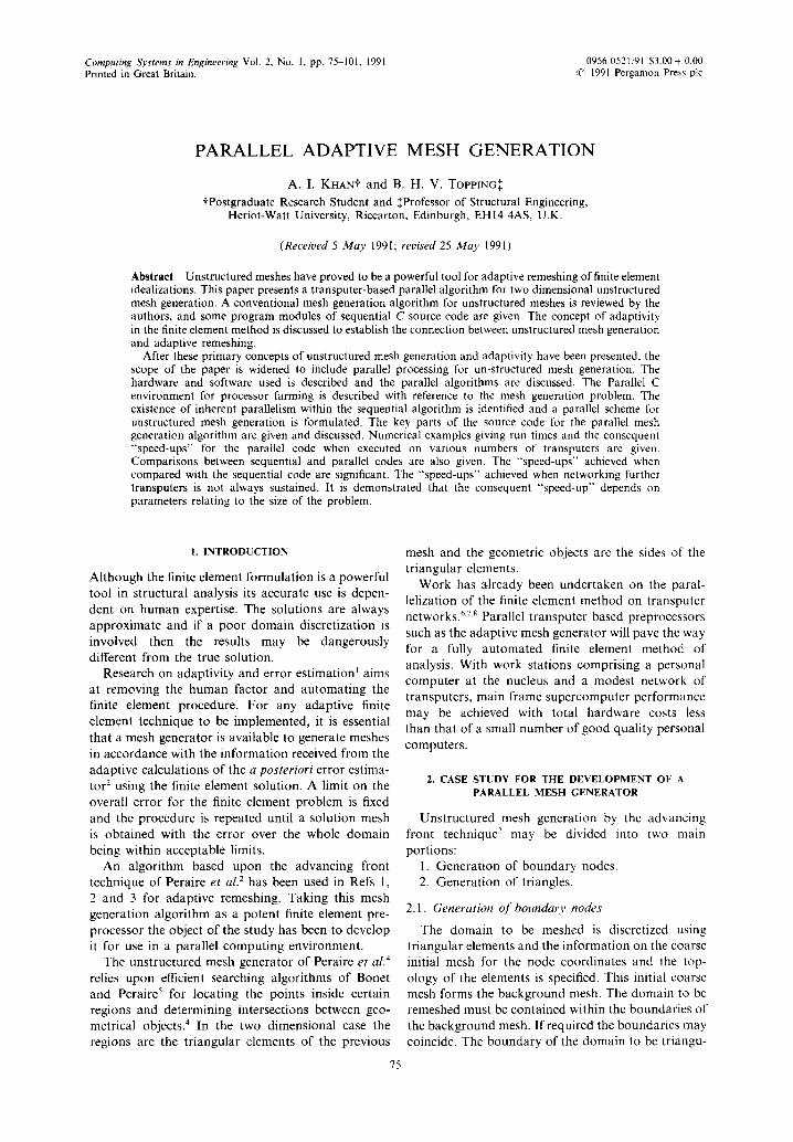
Fig. 1. Idealization of domains with internal boundaries as a boundary front.

lated is idealized as a loop, linking all the specified boundary nodes in counter-clockwise direction. If the domain contains any internal boundaries (openings or cut-outs) then the nodes on these internal boundaries are idealized as a loop linking them in a clockwise direction. This domain boundary discretization is done in accordance with the convention adopted by Lo. 9 The idealization of a square shaped domain containing an arbitrary internal boundary is shown in Fig. 1; this idealization is known as the boundary front. The mesh shown in Fig. 1 comprises two elements. This mesh would be referred to as the background mesh for the first re-meshing of this domain. In a subsequent remeshing the last generated mesh becomes the next background mesh.

The object of assigning a counter-clockwise numbering to external boundary nodes and clockwise numbering to internal boundary nodes is to guaran- tee that triangular elements generated by the algorithm, using the segments of the front as their base, will always form within the domain to be triangu- lated. When a boundary segment undergoes element generation, then only the nodes on the left side of the element are considered as probable candidates for forming the apex of the triangle if the afore-mentioned numbering conventions are used. The left side of a segment is determined from the nodal coordinates of the first and second nodes of the segment. As the node numbering on the segments is done in a particular order, say counter-clockwise for external boundary segments, therefore a vector having its direction set at 90 degrees counter-clockwise from the direction of the segment will define the space to the left of the external boundary segment. The nodes on the loop formed by the external boundary segments are numbered counter-clockwise so that the elements will form in the region enclosed by the external boundary segments. For the internal boundary segments it is required that the elements should form

outside the loop defined by the internal boundary segments and so the node numbering convention is reversed.

For a mesh generator designed for structural analysis where the optimum shape of the mesh elements is that of an equilateral triangle, the mesh parameter for the triangular mesh generator may be taken as the magnitude of the side length of the triangular mesh element to be generated in a particular region of the domain. Thus for each element i of the background mesh, a mesh parameter value 6(i) is assigned. The generation of nodes on each segment of the initial front is done in accordance with the theory presented by Peraire e t a l . 2 The algorithmic details are as follows:

1. For each node the 6 values for all associated elements are averaged. These nodal mesh parameter values are termed 6,. Thus for any node a having a total number of mesh elements connecting with it n a the associated nodal mesh parameter may be calculated as

y f la 1 (~ ( i ) ~.~ - - - ( 1 )

na

2. The intermediate nodes are generated from the end of the segment which has a higher value of 3, towards the end with the lower value. The intermediate node generation may be represented by the following set of simple equations:

L2 * ¢~ nx

Ll L2 + ~.x -- 6.2' (2)

a n d

( 6 ~ ) . e ~ - - [(¢~.x *LI ) + (~.2 *L2)]

L (3)

Parallel adaptive mesh generation 77

where, the greater nodal parameter value is termed &,~ and the lesser 6,2; L~ is the distance of each generated node from the first end; and L is the length of the segment. Also 6,x is the interpolated value of the mesh parameter at each generated node location, equal to 6,1 at the first end and then decreasing to 6,2 at the second end of the segment. The distance between the generated node and the second end is defined by L 2. Initially L 2 = L and 6,x = 6,,. This procedure is repeated provided L 2 > 6,2 , and the nodes are generated on the segment.

The node generation stops as soon as the available space to place the next node becomes less than 6,2. The last node generated is usually not in proportion to the local nodal mesh parameter values in that region. In such cases it is therefore necessary to distribute the last L 2 value over the previously generated intermediate segments, in proportion to their lengths. The last generated node is therefore deleted from the node list.

3. By repeating this procedure all over the segments of the initial boundary segments a front may be obtained, comprising straight line segments with the length of each segment in proportion to the local mesh parameter value.

2.2. boundnode

The function boundnode generates the nodes on the boundaries of a domain. The structure of the function is as follows:

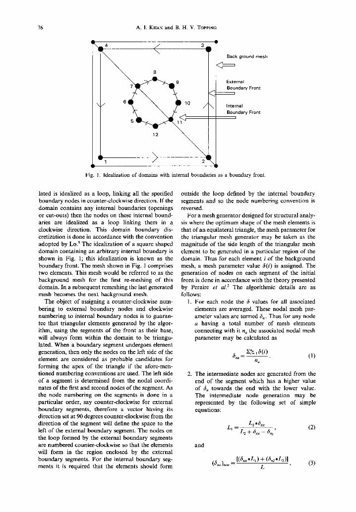
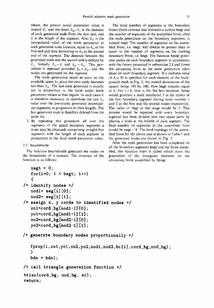
The total number of segments in the boundary fronts (both external and internal) is termed bsgt and the number of segments of the assembled front, after the node generation on the boundary segments, is termed nsgt. The number of segments on the assembled front, i.e. nsgt, will always be greater than or equal to the number of segments on the starting boundary front, i.e. bsgt. The function fprop generates nodes on each boundary segment in accordance with the theory presented in subsection 2.1 and forms the advancing front as the node generation takes place on each boundary segment. If a uniform value of 61 = 50 is specified for each element of the background mesh in Fig. 2, the overall dimensions of the square being 100 by 100, then bsot remains equal to 4. For i = 0, that is, for the first iteration, Iprop would generate a node numbered 5 at the center of the first boundary segment having node number 1 and 2 as the first and the second nodes respectively. The value of nsot at this stage would be 5. This process would be repeated until every boundary segment has been divided into two equal parls by placing a node at the middle of each segment. The final number of segments in the assembled front would be nsot = 8. The final topology of the assembled front for the above case is shown in Table 1 and the generated nodes are shown in Fig. 3.

After the node generation has been completed on all the boundary segments bsot and the front assembled, the function trian is called which starts the generation of the triangular elements on the advancing front assembled by fprop.

nsgt = O; for(i=O; i < bsgt; {

/* identify nodes */ nod1= seg[i][O]; nod2= seg[i][1];

/* assign x, y

xol=cord_bg yo1=cord_bg xo2=cord_bg yo2=cord_bg

i÷+)

cords to identified nodes */ [nod1-1] [0] ; [nod1-1] [1] ; [nod2-1] [0] ;

[nod2-1] [1] ;

/* generate boundary nodes proportionally */

fprop (i, xol. yol. xo2, yo2. nodl. nod2, bc [i]. cord_bg, nod_bg) ; }

bdn = bdnl;

/* call triangle generation function */

trian(cord_bg, nod_b E . ei) ; return ;

78 A. 1. KHAN and B. H. V. TOPPING

10

1 oo

L4 ( 3m"

\ ! (11 = 50

Back ground mesh / "1

External Boundary Front

Fig. 2. Background mesh and boundary front of a square-shaped domain.

7 / .. ( \ w

A / w 5

/ \

~| 6

/ \

\

3

Assembled Front

Fig. 3. Node generation with a uniform background mesh parameter of 6 i = 50.

Table 1. The nodal connectivities of the assembled front

nsgt First node Second node

1 1 5 2 5 2 3 2 6 4 6 3 5 3 7 6 7 4 7 4 8 8 8 1

2.3. Generation o f the triangular elements

The triangle generation scheme follows the scheme described by Peraire et al. 2'4 Features similar to those presented by Jin and Wieberg ~° for ensuring the

robustness of the algorithm have been included in the authors ' code.

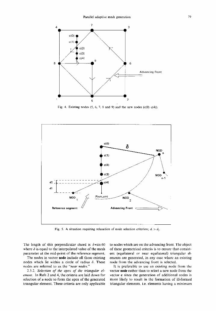
2.3.1. Identification o f candidate nodes for selection as an apex node. Triangular elements are generated by either identifying suitable existing nodes from the front and/or generating new nodes. The existing and the new nodes are shown in Fig. 4. The existing suitable nodes are stored in a vector node and the new nodes, generated along a line perpendicular to the segment, are stored in vector e. The node numbers in both these vectors are candidates for the apex node of the triangular element.

As shown in Figs 4 and 5, five equally spaced nodes, c(0)-c(4), are generated along a perpendicular chord from the mid-point of the reference segment.


7 3

• A A

c(0)

c(1)

i °`3' \ c14) 9 \

5

Advancing Front l

Fig. 4. Existing nodes (5, 6, 7, 8 and 9) and the new nodes (c(0)-c(4)).

dl

NOD 1 /

Reference segment

c(O)

c141

S

A d v a n c i n g F r o n t i ~

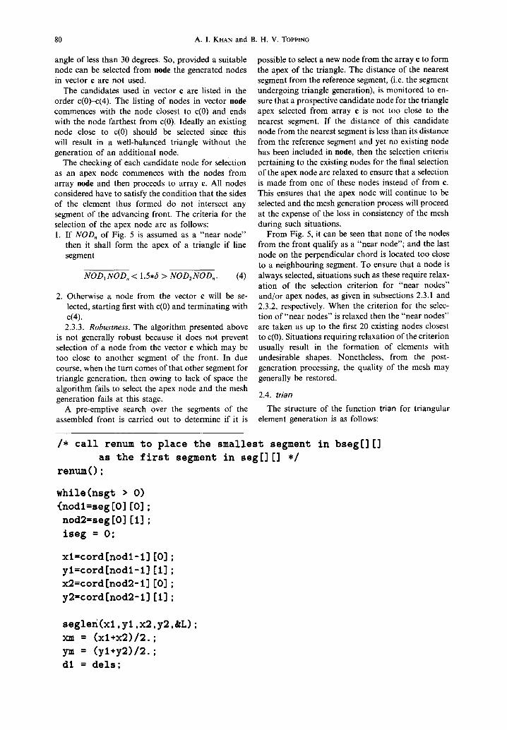
Fig. 5. A situation requiring relaxation of node selection criterion; d 1 > d 2.

The length of this perpendicular chord is 6 ,s in 60 where 3 is equal to the interpolated value of the mesh parameter at the mid-point of the reference segment.

The nodes in vector node include all those existing nodes which lie within a circle of radius 6. These nodes are referred to as the "'near nodes."

2.3.2. Selection of the apex of the triangular element. In Refs 2 and 4, the criteria are laid down for selection of a node to form the apex of the generated triangular element. These criteria are only applicable

to nodes which are on the advancing front. The object of these geometrical criteria is to ensure that consist- ent (equilateral or near equilateral) triangular elements are generated, in any case where an existing node from the advancing front is selected.

It is preferable to use an existing node from the vector node rather than to select a new node from the vector c since the generation of additional nodes is more likely to result in the formation of ill-formed triangular elements, i.e. elements having a minimum


angle of less than 30 degrees. So, provided a suitable node can be selected from node the generated nodes in vector c are not used.

The candidates used in vector e are listed in the order c(0)-c(4). The listing of nodes in vector node commences with the node closest to c(0) and ends with the node farthest from c(0). Ideally an existing node close to c(0) should be selected since this will result in a well-balanced triangle without the generation of an additional node.

The checking of each candidate node for selection as an apex node commences with the nodes from array node and then proceeds to array c. All nodes considered have to satisfy the condition that the sides of the element thus formed do not intersect any segment of the advancing front. The criteria for the selection of the apex node are as follows: 1. If N O D n of Fig. 5 is assumed as a "near node"

then it shall form the apex of a triangle if line segment

N O D ~ N O D n < 1.5,6 > N O D 2 N O D n. (4)

2. Otherwise a node from the vector c will be selected, starting first with c(0) and terminating with c(4). 2.3.3. Robus tness . The algorithm presented above

is not generally robust because it does not prevent selection of a node from the vector e which may be too close to another segment of the front. In due course, when the turn comes of that other segment for triangle generation, then owing to lack of space the algorithm fails to select the apex node and the mesh generation fails at this stage.

A pre-emptive search over the segments of the assembled front is carried out to determine if it is

possible to select a new node from the array e to form the apex of the triangle. The distance of the nearest segment from the reference segment, (i.e. the segment undergoing triangle generation), is monitored to ensure that a prospective candidate node for the triangle apex selected from array c is not too close to the nearest segment. If the distance of this candidate node from the nearest segment is less than its distance from the reference segment and yet no existing node has been included in node, then the selection criteria pertaining to the existing nodes for the final selection of the apex node are relaxed to ensure that a selection is made from one of these nodes instead of from c. This ensures that the apex node will continue to be selected and the mesh generation process will proceed at the expense of the loss in consistency of the mesh during such situations.

From Fig. 5, it can be seen that none of the nodes from the front qualify as a "near node"; and the last node on the perpendicular chord is located too close to a neighbouring segment. To ensure that a node is always selected, situations such as these require relaxation of the selection criterion for "near nodes" and/or apex nodes, as given in subsections 2.3.1 and 2.3.2, respectively. When the criterion for the selection of "near nodes" is relaxed then the "near nodes" are taken as up to the first 20 existing nodes closest to c(0). Situations requiring relaxation of the criterion usually result in the formation of elements with undesirable shapes. Nonetheless, from the post- generation processing, the quality of the mesh may generally be restored.

2.4. trian

The structure of the function trian for triangular element generation is as follows:

/* call renum to place the smallest segment as the first segment in seg[] [] */

renum() ;

in bseg[] []

while(nsgt > O) {nodl=seg[O][O]; nod2=seg[O][l]; iseg = O;

xl=cord[nodl-1] [0] ;

yl=cord[nodl-1] [1] ;

x2=cord [nod2-1] [0];

y2=cord[nod2-1] [1] ;

seglen(xl,yi,x2,y2,kL); xm = (x/+x2)12.;

ym = (yl+y2)12.;

dl = dels;

Parallel adaptive mesh generation

search_elbgl(xm,ym,&dl, cord_bg, nod_bg, el);

81

seldel(dl, L. kselde11);

perpcord(xl,yl,x2,y2,seldell,ccc);

for(i=O; i < 20; i++)

node [i] = 0 ;

nearnode(nodl.nod2,ccc[O] [0], ccc[O] [l].node,seldell, &test_sel);

test_dis = pt_dist(xl.yl,x2.y2.ccc.ccc[4][O],ccc[4][l]);

/* test_sel = 1 indicates that no near node has been selected

test_dis = I indicates that the node from ccc is too close

to a segment of the front. So a near node is required relaxing

the condition of node being within a specified radius */

if(test_sel == I && test_dis == 1) {

for(i=O; i < 20; i++)

node[i] = O;

nearnode_ult(nodl,nod2,ccc[O][O], ccc[O][l],node);

test_sel = -1; }

cri = 1.5;

selnod=selnode(PER,cri,iseg,seldell,nodl.nod2.ccc,node,test_sel);

if(selnod == -I) {

for(i=O; i < 20; i++)

node[i] = O;

nearnode_ult(nodl.nod2,ccc[O][O], ccc[O][1],node);

selnod=selnode_drs(iseg,nodl,nod2,ccc.node): }

if(selnod == -i) {

break; }

en++;

prune(selnod.iseg,en_i, en_f. seldell);

if(nsgt == O)

break;

renum () ; }


n n = b d n l ;

n e = e n ;

r e t u r n ;

The function r e n u m renumbers the advancing front by making the shortest segment of the front the first segment. The length of this segment is calculated by seglen and the coordinates of its mid-point are calculated as xm ym. The function search elbgl calculates the mesh parameter value 6 by locating (xm, ym) within an element of the background mesh and then interpolating the value of the mesh parameter from the nodal mesh parameters 6, of the background' mesh element; perpcord generates a line from (xm, ym) of length 6 ,s in60 to the left of the segment and divides it into five equal parts by placing intermediate nodes whose coordinates are stored in a two dimensional array eec. The function nearnode checks all the nodes on the front (except those on the reference segment) with respect to their distances from the tip of the perpendicular chord generated by perpcord, the nodes equal to or closer than 6 being stored in the vector node. The function pt_dist identifies when another segment of the front is close to the reference segment, as shown in Fig. 5, and returns a ' + 1' value if dr > d2. If no "near node" has been selected and pt_dist returns '1' then the condition for all nodes less than or equal to 6 units away from the tip c(0) of the perpendicular chord is relaxed for the selection of "near nodes" and function nearnode_ult is called. This selects the "near nodes" as the first twenty nodes closest to the tip of the perpendicular chord.

The function selnode selects a node for the formation of the apex of the triangle from the list of "near nodes": i.e. node, on the front and the nodes generated on the perpendicular chord eee. This function also checks that the "near nodes" are only on the left side of the segment and that the generated sides of the triangle do not intersect any side of the current front. In an extreme case, when the values of the mesh parameter show large variations over a short distance, then it is possible that selnode cannot select a node. The function then returns a ' - 1' value and the program then calls selnode_drs which obliges the program to select a node from the existing front or from new nodes, as the case may be. The only consideration here is that the selected node must not form an element the sides of which intersect with any segment on the front. The element in this case may have an inconsistent shape. The function prune re- moves the inactive sides from the front. The inactive sides on the front are the ones which cannot form sides of a new triangle.

The above steps are repeated until the number of segments in the advancing front, nsgt, becomes equal to zero.

3. POST-PROCESSING OF THE MESH

The post-processing procedures from Ref. 4 for restoring the consistency of the mesh generated are given below.

3.1. Diagonal exchange

After the generation of the mesh, first post-processing is undertaken by performing diagonal exchange between two elements where necessary. Each element of the generated mesh is considered in turn and the element adjacent to its longest side identified. The minimum angle from the angles subtended by the pair of elements is determined. The diagonal is swapped. Again, the minimum angle for the new topologies is calculated and if the minimum angle is found larger in the latter case then the new topology is adopted; otherwise the old topology of the elements is main- tained.

3.2. Smoothing

For each interior node of the generated mesh all the nodes connecting through an element side are identified. The x and y coordinates of all these nodes are averaged and these averaged nodal coordinates are assigned as the new coordinates for the node under consideration. This process is repeated a number of times for all the interior nodes of the mesh. In the examples presented in this paper the smoothing was done five times for each new mesh.

4. ADAPTIVITY

4.1. Introduction

In the case of finite element idealizations based upon simple constant-strain triangular elements the accuracy of the results depends upon the topology of the mesh chosen for the finite element analysis. Adaptive remeshing can predict an efficient mesh by taking into account the domain error for a uniformly graded mesh. An efficient mesh is defined as the one in which the error is equally distributed over the domain.

Through adaptive remeshing the domain error is reduced as well as uniformly distributed over the domain. The analyses are carried out until the domain error becomes less than a pre-defined error value.

4.2. Domain error

For a constant-strain triangular element the el- emental stresses obtained from a finite element analy-


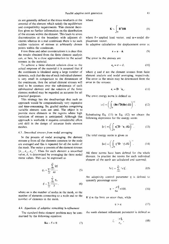
sis are generally defined as the stress resultants at the centroid of the element which satisfy the equilibrium and compatibility requirements. This element therefore gives no further information on the distribution of the stresses within the element. This leads to stress discontinuities at the boundary with adjacent elements whereas in a real continuum there is no such sudden variation of stresses at arbitrarily chosen points within the continuum.

From these and other considerations it is clear that the results obtained from the finite element analysis can, at best, be a close approximation to the actual stresses in the material.

To achieve a finite element solution close to the actual response of the material it is assumed that if the continuum is idealized using a large number of elements, such that the size of each individual element is very small in comparison to the dimensions of the continuum, then the actual element stresses will tend to be constant over the sub-domain of each infinitesimal element and the solution of the finite element method may be regarded as accurate for all practical purposes.

This strategy has the disadvantage that such an approach would be computationally very expensive and time-consuming. So, graded meshes comprising variable element sizes are used. The object is to provide more elements in the regions where high variation of stresses is anticipated. Although this approach is workable it requires considerable effort and skill in the design of accurate finite element meshes.

4.3.. Smoothed stresses from nodal averaging

In the process of nodal averaging, the element stresses q from all the elements common to the node are averaged and this is repeated for all the nodes of the mesh. The vector q consists of the element stresses { G , G.~, G~.} r" Then for each element a smoothed value, d, is determined by averaging the three nodal stress values. This can be expressed as

~ _ n = ~ i= l (5) nn n s

3

_ ~ ( 6 ) ne

where nn is the number of nodes in the mesh, ns the number of elements connecting to a node and ne the number of elements in the mesh.

4.4. Equations of adaptive remeshing h-refinement

The standard finite element problem may be sum- marized by the following equation:

K u - - f = 0 ( 7 )

where

K = I ~ B r D B (8)

where f--applied load vector, and u = nodal displacement vector. In adaptive calculations the displacement error is:

e = u - ft. ( 9 )

The error in the stresses are

e . = q - q , ( 1 0 )

where q and q are the element stresses from finite element analysis and nodal averaging, respectively. The error in the strain may be determined from the error in the stresses:

e , = D le o . (11)

The error energy norm is defined as

, ,eH=(fo (Be)VD(Be) d ~ ) ~2 (12)

Substituting Eq. (11) in Eq. (12) we obtain the following expression for the energy norm:

,=t oe o,do) The total energy norm is given as

(;o Hull= qrD t _6- df~ . (14)

All these norms have been defined for the. whole domain. In practice the norms for each individual element of the mesh are calculated and summed:

z 11ell = ~ Ilell~. (15)

i=1

An adaptivity control parameter ~ is defined to quantify percentage error

ILel[ *100. (16) ~ = ~

If q is the limit on error then, while

> q (17)

the mesh element refinement parameter is defined as

Ilell; ~, - , ( 1 8 )

em

84 A.I. KhAN and B. H. V. TOPPING

where

= ~(]lullZy/2. (19) em \ ne .]

The mesh is refined according to

hnew =-,h+ (20)

until

q ~< q, (21)

where h i and hne w a r e the previous and the new element sizes determined from the adaptive analysis. The symbol hne w corresponds to 6 (i) in subsection 2.1.

4.5. Discussion on some approaches to adaptivity

The adaptive remeshing method shown above may be divided into three parts; namely, (i) calculation of smoothed stresses, (ii) calculation of norms for representing the domain errors, and (iii) transformation of the domain errors to mesh parameters, for remeshing.

For part (i) Sibia and Hinton 3 have used the method of nodal averaging as described previously. Zienkiewicz and Zhu j have used a more sophisticated approach wherein the smoothing is done over the sub-domain of each element by assigning the same interpolation function as the element displacement function. This is shown in Eqs (16), (17) and (18) of Ref. I.

With regard to part (ii), the error energy norm ppe II is determined in the same way in both the papers, L3 and the notation used is also the same. However in the paper by Zienkiewicz and Zhu 1 the total energy norm Ilu II has not been clearly defined. It is, however, assumed that it carries the same meaning as IIw*dl in Ref. 3. The norm IIw*l[ of Ref. 3 is synonymous with Ilu[[ in this text.

For part (iii) different approaches have been adopted in Refs 1 and 3 for evaluating the term em. In Eq. (8) of Ref. 3 this term is called ~ and is taken as fi = r7 II w* II/n ~/2 where n is the number of elements in the domain.

Zienkiewicz and Zhu 1 have calculated this term on a "Root Mean Square" basis as shown in Eq. (24) of Ref. 1 and Eq. (19) of this text. Both these approaches have been tested for constant strain triangular element and it appears that the approach in Ref. 1 gives better smoothness for the mesh generation parameters. It may be pointed out that if non-smooth values of mesh parameters, exhibiting large variations in parameter values in local domains, are encountered then this may lead to the breakdown of the mesh regeneration algorithm.

5. HARDWARE CONFIGURATION

The description of the hardware used in the development and running of the parallel adaptive mesh

Table 2. Hardware used in the parallel adaptive mesh generator

No. of Component specifications of units

IMST800 transputer 12 TTM18 TRAM with 8MB dynamic RAM 1 TTM3 TRAM with 1 MB dynamic RAM 11 Transtech mother board TMB08 1 Transtech mother board TMBI2 1 Transrack for housing TMB12 1

generator is given in Table 2. All the daughter boards TTM18 and TTM3 support IMST800 transputers. The TTM18 and TTM3 daughter boards have 8 MBytes and 1 MBytes of on-board memory, respectively. The TTM18 daughter board was plugged into the TMB08 mother board and acted as the root. The TMB08 mother board was fixed into the expansion card slot of a PC-AT compatible. The Down, Config- Down and the PipeTail IL12 from the TMB08 were connected to the UP, ConfigUP and PipeHead of the TMB12. The TMB12 was populated with 11 TTM3 TRAMS acting as slaves to the root transputer. The INMOS Link speeds ~3 on both the mother boards were set to high i.e. 20 Mbits/sec. The TMB12 was mounted in a Transrack. The Transrack has pro- vision for 10 large slots for TMB12 mother boards. Each board may be populated with up to 16 TTM3 daughter boards. In theory, therefore, the Transrack may support 160 TTM3 daughter boards.

The transputers are connected in series with link 2 of the first transputer connected to link 1 of the second transputer and so on. This linear serial configuration is present in hard-wired form on the TMB08 and TMB12 mother boards. Futher information on the default pipelines of TMB08 and TMBI2 mother boards may be obtained from Refs 11 and 12.

6. PARALLEL COMPILER

OCCAM ~+ is a language developed for supporting concurrent processes. Transputer systems may be designed and programmed using OCCAM which allows setting up of concurrent processes, for applications, communicating through channels. Since OC- CAM was developed for the transputer environment it would therefore be reasonable to assume that OCCAM would be a strong candidate for writing a parallel transputer-based code. However, with the availability of parallel compilers for popular languages like C and FORTRAN, which support most of the standard features of their sequential counterparts, it requires a great deal less effort to create a parallel version if the sequential code has already been developed in C or FORTRAN.

The sequential code for un-structured mesh generation was written in C. The 3L Parallel C compiler 15 was therefore selected for the development of the parallel code.


• i

6

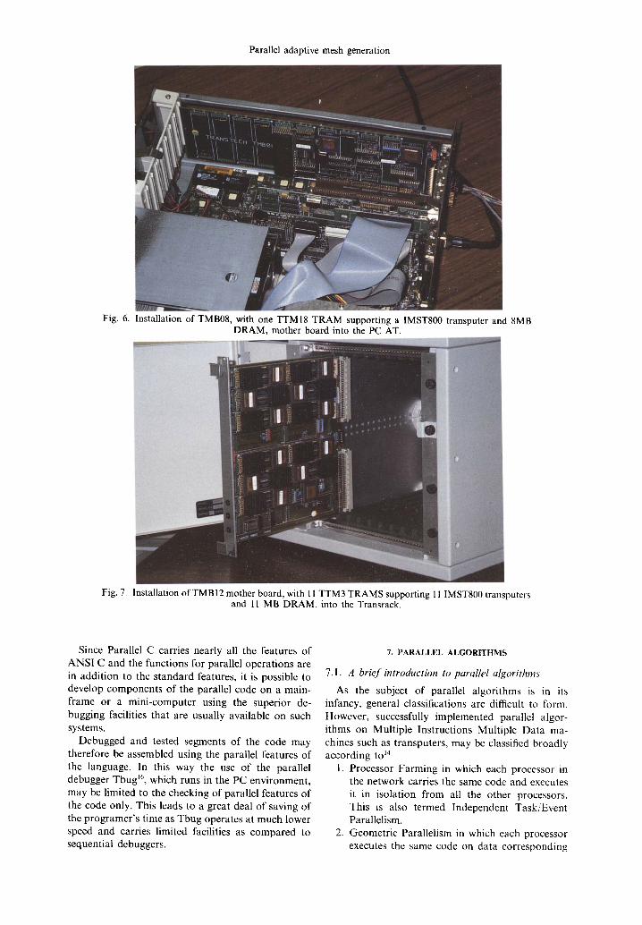
Fig. 6. Installation of TMB08, with one TTMI8 TRAM supporting a IMST800 transputer and 8MB DRAM, mother board into the PC AT.

Fig. 7. Installation of TMB12 mother board, with 11 TTM3 TRAMS supporting 11 IMST800 transputers and 11 MB DRAM, into the Transrack.

Since Parallel C carries nearly all the features of ANSI C and the functions for parallel operations are in addition to the standard features, it is possible to develop components of the parallel code on a main- frame or a mini-computer using the superior de- bugging facilities that are usually available on such systems.

Debugged and tested segments of the code may therefore be assembled using the parallel features of the language. In this way the use of the parallel debugger Tbug 16, which runs in the PC environment, may be limited to the checking of parallel features of the code only. This leads to a great deal of saving of the programer's time as Tbug operates at much lower speed and carries limited facilities as compared to sequential debuggers.

7. P A R A L L E L A L G O R I T H M S

7.1. A brief introduction to parallel algorithms

As the subject of parallel algorithms is in its infancy, general classifications are difficult to form. However, successfully implemented parallel algorithms on Multiple Instructions Multiple Data ma- chines such as transputers, may be classified broadly a c c o r d i n g to 14

1. Processor Farming in which each processor in the network carries the same code and executes it in isolation from all the other processors. This is also termed Independent Task/Event Parallelism.

2. Geometric Parallelism in which each processor executes the same code on data corresponding

86 A. I. KHAN and B. H. V. TOPPING t

to a sub-region of the system being simulated and communicates, boundary data to neighbouring processors handling neighbouring sub- regions.

3. Algorithmic Parallelism in which each processor is responsible for part of the algorithm, and all the data passes through each processor.

7.2. Processor farming in 3L Parallel C

The processor farming environment in Parallel C 15 is generated by the flood-fill configurer. The flood-fill configurer provided with the 3L Parallel C compiler enables the programmer to implement a processor farming application which is completely portable over transputer networks having a different number of transputers and/or topologies. Any flood-fill application must have the following program structure:

1. A master task to divide the job into independent work packets;

2. A worker task which is loaded on to each node (processor) of the network; and

3. A configuration file describing the memory requirements and other attributes of the tasks.

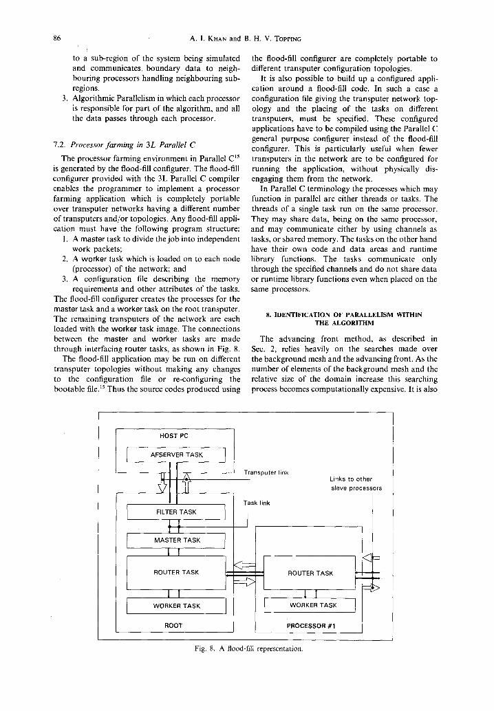
The flood-fill configurer creates the processes for the master task and a worker task on the root transputer. The remaining transputers of the network are each loaded with the worker task image. The connections between the master and worker tasks are made through interfacing router tasks, as shown in Fig. 8.

The flood-fill application may be run on different transputer topologies without making any changes to the configuration file or re-configuring the bootable file. 15 Thus the source codes produced using

the flood-fill configurer are completely portable to different transputer configuration topologies.

It is also possible to build up a configured application around a flood-fill code. In such a case a configuration file giving the transputer network topology and the placing of the tasks on different transputers, must be specified. These configured applications have to be compiled using the Parallel C general purpose configurer instead of the flood-fill configurer. This is particularly useful when fewer transputers in the network are to be configured for running the application, without physically dis- engaging them from the network.

In Parallel C terminology the processes which may function in parallel are either threads or tasks. The threads of a single task run on the same processor. They may share data, being on the same processor, and may communicate either by using channels as tasks, or shared memory. The tasks on the other hand have their own code and data areas and runtime library functions. The tasks communicate only through the specified channels and do not share data or runtime library functions even when placed on the same processors.

8. IDENTIFICATION OF P A R A L L E L I S M WITHIN THE A L G O R I T H M

The advancing front method, as described in Sec. 2, relies heavily on the searches made over the background mesh and the advancing front. As the number of elements of the background mesh and the relative size of the domain increase this searching process becomes computationally expensive. It is also

HOST PC

I AFSERVER TASK

iJ + []-f FILTER TASK

i t I [

MASTER TASK

I !

ROUTER TASK

I I WORKER TASK

ROOT

Transputer link

Task link

ROUTER TASK

I 1 WORKER TASK

PROCESSOR #1

J l

Links to other slave processors

Fig. 8. A flood-fill representation.

Parallel adaptive

noted that mesh generation may be carried out on different sub-domains independently. If the domain to be remeshed is considered as comprising loops of external and internal boundary segments, then each sub-domain may be visualized as an external boundary loop occurring completely within the remeshing region of the domain. The area enclosed by the external and internal boundary loops of the domain is called the remeshing region.

These sub-domains fully cover the remeshing zone of the domain and the boundary segments of these sub-domains do not intersect with one another.

Computational advantages may be derived through parallelism in the following ways:

(a) By adopting parallel searching techniques; or (b) By dividing the domain into suitable sub-do-

mains and mapping these sub-domains onto different processors.

Scheme (a) would retain all the characteristics of the original algorithm but the actual process of boundary discretization and that of element generation would remain sequential. In scheme (b) the actual mesh generation process would be done in parallel and the algorithm would not require communication between slave processors, as each individual slave processor would be entrusted with a separate sub-domain. However, the generation of elements larger than the specified sub-domain would not be possible in this case.

For the implementation of this scheme, account was taken of the following points:

1. The discretized background mesh, representing the domain, has to be divided into separate sub-domains in order to be mapped onto different processors. The size and shape of each sub- domain should be such as to ensure adequate load balancing of the processors for optimizing efficiency.

2. The integrity of the boundary connectivities between the meshes generated on separate processors has to be be guaranteed.

3. After the parallel processing of the sub-domains the assembly of the sub-domain meshes to form the full domain mesh must be considered.

As mentioned above, the execution rate of the advancing front technique depends heavily on the searches made over the background mesh elements and the segments of the advancing front. So if scheme (b) were to be selected then the computational advantage would be two-fold:

1. Owing to the division of the domain into smaller sub-domains the advancing fronts of each sub- domain would have a smaller number of segments as compared to the case if the whole domain was idealized as a single loop. Thus the geometric searching effort required to generate an element within a sub-domain would be reduced in proportion to the ratio between the size of the sub-domain and the domain.

From the theory presented in Sec. 2, the mesh

mesh generation 87

parameter 6 is specified for each element of the background mesh. If the division of the background mesh was done element-wise, meaning that each element of the background mesh was treated as a separate sub-domain, then for all such triangular sub-domains the 6 and 6, values would be known at all times. Thus, the requirement to search over the background mesh, to determine the local values of mesh parameters, would be eliminated.

2. As each sub-domain undergoes independent generation of elements, the actual process of element generation would occur simultaneously, in different regions of the domain.

Scheme (b) therefore provides computational advantages owing to the smaller number of segments of the advancing front per sub-domain and Independent Task/Event Parallelism. As the scheme does not require inter-processor communication a processor farming environment generated by the flood-fill configurer ~5 was selected for the development of the scheme. This also added to the simplicity and portability of the code.

9. SUB-DOMAIN DISCRETIZATION

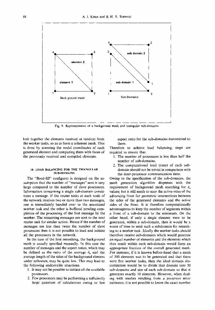
A two dimensional domain is divided into triangular elements of similar size. This initial mesh is termed the background mesh. Figure 9 shows a coarse background mesh comprising only two elements for remeshing of a square domain. For each element of this background mesh, a mesh parameter value 6 is specified. From Eq. (1) the nodal mesh parameters 6,, are calculated.

As each sub-domain is to be meshed individually on a separate processor and the topology of each sub-domain is known to be triangular, the boundary nodes in all the sub-domains may be numbered identically and in the same order, as shown in Fig. 9. This eliminates the need for the transmission of the information on the number and the connectivities of the boundary segments of each sub-domain. Each processor is "aware" of the fact that each sub-domain which it will receive will comprise three nodes and it accordingly assigns the boundary connectivities in a counter-clockwise manner. In order to initiate mesh generation on any processor, only the nodal coordinates and the nodal mesh parameter values need to be transmitted from the master task. If the actual node numbers and the topologies of each sub-domain had been sent to the processors, then inter-processor communication would be required every time a new node was created within any sub-domain. The simple representation shown in Fig. 9 allows independent generation of nodes and elements within each sub- domain without the restriction of an overall node numbering protocol. All the nodes within each sub- domain are numbered from "1" onwards. It becomes the task of the overall mesh assembler to successfully


4 A

i v v

2

Back ground mesh

3 3

3

w

Sub Domains

Fig. 9. Representation of a background mesh and triangular sub-domains.

knit together the elements received at random from the worker tasks, so as to form a coherent mesh. This is done by scanning the nodal coordinates of each generated element and comparing them with those of the previously received and compiled elements.

10. LOAD BALANCING FOR THE TRIANGULAR SUB-DOMAINS

The "flood-fill" configurer is designed on the as- sumption that the number of "messages" sent is very large compared to the number of slave processors. Information concerning a single sub-domain consti- tutes a message. If the router tasks at each node of the network receives two or more than two messages, one is immediately handed over to the associated worker task and the other is buffered pending completion of the processing of the first message by the worker. The remaining messages are sent to the next router task for similar action. Hence if the number of messages are less than twice the number of slave processors then it is not possible to load and initiate all the processors in the network.

In the case of the first remeshing, the background mesh is usually specified manually. In this case the number of messages and the aspect ratios, which may be defined as the ratio of the average f, and the average length of the sides of the background element under reference, may be quite low. This may lead to the following undesirable situations.

1. It may not be possible to initiate all the available processors.

2. Few processors may be performing a sufficiently large quantum of calculations owing to low

aspect ratio for the sub-domains transmitted to them.

Therefore to achieve load balancing, steps are required to ensure that:

1. The number of processors is less than half the number of sub-domains.

2. The computational load (time) of each sub- domain should not be trivial in comparison with the inter-processor communication time.

Owing to the specification of the sub-domains, the mesh generation algorithm dispenses with the requirement of background mesh searching for 6, values; but it still needs to scan the active sides of the advancing front for geometric intersections between the sides of the generated elements and the active sides of the front. It is therefore computationally advantageous to keep the number of segments within a front of a sub-domain to the minimum. On the other hand, if only a single element were to be generated, within a sub-domain, then it would be a waste of time to send such a subdomain for remeshing to a worker task. Ideally the worker tasks should therefore receive sub-domains which would generate an equal number of elements and the elements which thus result within each sub-domain would form an appropriate fraction of the overall generated mesh. For instance, if it is known before-hand that a mesh of 500 elements was to be generated and that there were five worker tasks, then the ideal domain discretization would be to divide that domain into 50 sub-domains and size of each sub-domain so that it generates exactly I0 elements. However, when deal- ing with meshes resulting from a posteriori error estimates, it is not possible to know the exact number


of elements that will be generated. A compromise therefore has to be made between ideal load balancing and the extent of load balancing that may be achieved by not adding excessive computational overheads.

The load balancing techniques outlined in this section target the sub-domains having either the ability to generate a large number of elements or the inability to generate any elements at all. The prolific elements are subdivided, subject to certain geometric preconditions and the non-generative elements are sent straight away for compilation without being sent to the worker tasks. If

In order to alleviate the load imbalancing situations discussed above, the background mesh is processed through two mesh filters. These filters check the background mesh (sub-domains) for their ability to generate a large number of elements or no elements at all, within each sub-domain. The filters have therefore been termed "Prolific Element Filter" or PE filter and "Non-Generative Element Filter" or NGE filter, respectively.

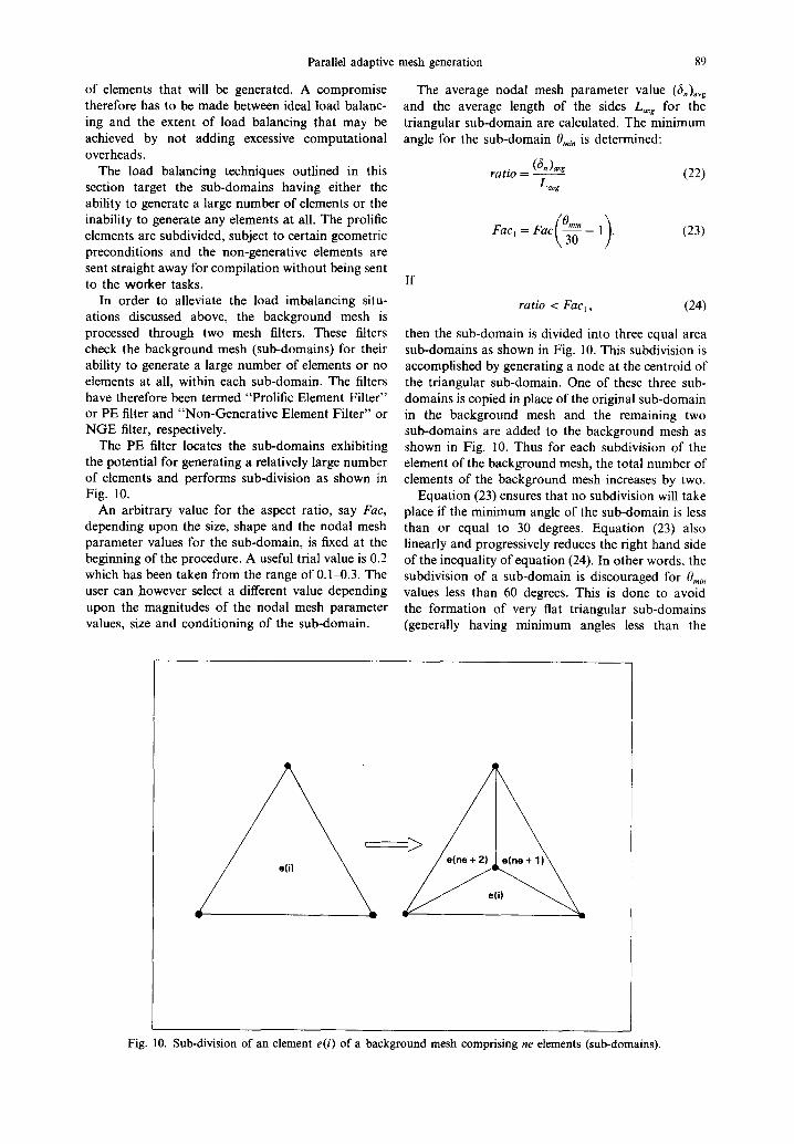
The PE filter locates the sub-domains exhibiting the potential for generating a relatively large number of elements and performs sub-division as shown in Fig. 10.

An arbitrary value for the aspect ratio, say Fac, depending upon the size, shape and the nodal mesh parameter values for the sub-domain, is fixed at the beginning of the procedure. A useful trial value is 0.2 which has been taken from the range of 0.14).3. The user can however select a different value depending upon the magnitudes of the nodal mesh parameter values, size and conditioning of the sub-domain.

89

The average nodal mesh parameter value (6,)avg and the average length of the sides Lavg for the triangular sub-domain are calculated. The minimum angle for the sub-domain Om~, is determined:

ratio - ( 6 n ) a v g (22) L avg

/ Omi n ,)

ratio < Facl, (24)

then the sub-domain is divided into three equal area sub-domains as shown in Fig. 10. This subdivision is accomplished by generating a node at the centroid of the triangular sub-domain. One of these three sub- domains is copied in place of the original sub-domain in the background mesh and the remaining two sub-domains are added to the background mesh as shown in Fig. 10. Thus for each subdivision of the element of the background mesh, the total number of elements of the background mesh increases by two.

Equation (23) ensures that no subdivision will take place if the minimum angle of the sub-domain is less than or equal to 30 degrees. Equation (23) also linearly and progressively reduces the right hand side of the inequality of equation (24). In other words, the subdivision of a sub-domain is discouraged for 0m~ n values less than 60 degrees. This is done to avoid the formation of very flat triangular sub-domains (generally having minimum angles less than the

v v v w

Fig. I0. Sub-division of an element e(i) of a background mesh comprising ne elements (sub-domains).


15-20 degree range), within the sub-domain under consideration.

The NGE filter is designed to locate sub-domains which will not generate mesh elements owing to their relatively higher nodal mesh parameter values as compared to their sub-domain sizes.

For each sub-domain (element) of the background mesh all three sides of the triangular sub-domain are checked for the nodal mesh parameter values at each end. The lesser of the two end values for each side of the triangular sub-domains are stored a s (~n)min"

If each entry in the (6~)mi, vector is greater than 51% of the length of the corresponding side of the sub-domain, then from the theory presented in subsection 2.1 it may be concluded that no intermediate node generation will take place on any of the boundary sides of the sub-domain. Hence no element generation would take place within the sub-domain. The NGE filter guarantees that the selected element will not undergo mesh generation within its sub- domain. It marks such an element and stores it in the location where the new mesh would be assembled. This filter does not however eliminate the possibility that some other elements which have passed through the filter unmarked, shall not undergo mesh generation.

I t . COMPATIBILITY BETWEEN ADJACENT SUB-DOMAINS

Since the adjacent elements (sub-domains) of the background mesh share the same nodal mesh parameter values 6, at the common nodes, and the discretization of the boundary segments of the sub- domains is carried out from the higher value of ~, to its lower value in Eq. (2), the common boundaries of the adjacent sub-domains will always have the same number and distribution of the intermediate generated nodes. Thus the connectivity of the adjacent sub-domains is guaranteed even when they are processed in isolation from each other.

12. MASTER TASK

In accordance with the flood-fill configuration requirements the parallel mesh generator is written in the form of a master task and a worker task. The master task performs the following functions:

1. The function main of the master task creates two parallel processes (threads), arbitrarily named as bound.send and bound_receive for handling communication with the worker tasks. These threads are synchronized using a semaphore.17

2. The thread main of the master task applies the PE and NGE filters to the background mesh and this is called the "preprocessing" procedure.

3. The thread bound-send contains the function

t The function net.broadcast is a new prototype version of the net.send function currently available with the 3L Parallel C Version 2.1 compiler.

net.broadcastt which transmits the information packet pertaining to each sub-domain. Only the sub-domains which have remained unmarked while passing through the NGE filter are transmitted. The router tasks distribute these packets among the idle worker tasks. Whenever the network of worker tasks becomes fully engaged the net_broadcast is blocked until a router task with an empty buffer becomes available.

The information on the nodal coordinates and the nodal mesh parameters 6, of a sub- domain is read into a "structure" type buffer by the thread. The function net_broadcast relays the information held in the pointed buffer in packets of 1024 bytes. The total length of the message in this case works out at less than 100 bytes; hence each message is carried within a single packet. Thus the terms "message" and "packet" have been used in a synonymous sense.

4. The thread bound.receive contains the function net-receive. The results from the worker tasks are received and net-receive waits until the next packet from the worker task becomes available. The net.receive is performed within a never ending loop.

5. In the case of a break down of the mesh generation algorithm within a worker task, an error message is received and displayed by the master task.

6. The main executes the function thread- deschedule within a loop while the worker tasks are active and are receiving and sending the information packets through net_broadcast and net_send to the main. This function causes main to be momentarily unable to execute (usually for one timer tick); causing main to be de-scheduled from the processor, thus allowing some other thread to resume execution in its place. This prevents main from hogging the processor to the detriment of the other two threads. In effect a very low priority level is achieved for the thread main and the benefit of processor scheduling is given to the bound_ send and bound.receive threads.

7. The information packets received from the workers are fitted into the overall mesh by bound_receive.

8. The post processing of the mesh by diagonal exchange and smoothing, as described in Ref. 4, is undertaken by main of the master task after all the sub-domains have been received back from the worker tasks.

The function net.broadcast and net_receive are performed in parallel with the thread main of the master task. This prevents the incoming result packets being blocked by the net_broadcast waiting for a worker to become free, or net_broadcast being blocked by net_receive waiting for output from the worker tasks.


12.1. Representation of the function main of the master task

s e m a _ i n i t ( k g r e e n , O) ; /* begin time count for preprocessing */

time (~ima) ;

/* average the b E mesh pars at each node */

node_pars () ;

store_bg(kn_iln); /* store b E mesh */

signal = O; /* count time at the end of pre- process k starts

for parallel processing */

time (~timb) ;

thread_c reate (bound_send, 1000, I, be) ;

thread_create (bound_receive, I000.0) ;

sema_signal (kgreen),

/* thread bound_send and bound_receive are activated here */

/ * w a i t h e r e t i l l r e s u l t s are r e c e i v e d * /

w h i l e ( s i g n a l < (ne_bg - k n t _ b g ) ) / * l e s s t h e e l s a l r e a d y p _ s t a c k * /

{ t h r e a d _ d e s c h e d u l e ( ) ;

if(ok_fail < O)

(printf("Packet no ~d failed at elem no = ~d\n".id_num,-l*ck_fail);

ne_bg = nel; knt_bg = O; write_info();

exit (I) ; } }

/* count time at end of parallel process */

time (A~im2) ;

un_load_st () ;

interdiag() ;

search_node () ;

for(i = O; i < 5; i++)

smooth1 () ;

The threads are synchronized by the semaphore green. The function sema_init assigns a starting value to the semaphore green as "0". A thread may only execute through a semaphore when the semaphore value is greater than zero. The function time returns the number of secs elapsed since a datum which is taken as 00:00:00 GMT on 1st of January 1970 by the Parallel C compiler, according to the host system clock. The function node_pars calculates the 6, using Eq. (1). The function s tore-bg stores the background mesh and also applies the PE and NGE filters. The integer variable knt_bg is equal to the number of the elements of the back-ground mesh marked by the NGE filter. The integer variable signal

is increased by one each time a worker task indicates that it has completed the remeshing of the sub- domain with which it was entrusted. The function thread_create establishes two threads for sending and receiving the packets to and from the worker tasks. As all necessary procedures stand completed at this stage sema.signal is called and bound . send which was waiting due to the '0' value of green, is activated. The bound-send sends the information packets to the worker tasks and the bound_receive becomes active as soon as it receives an output from a worker. It then increments the signal by one and fits the received elements into the mesh being compiled. During this period, when bound_send and bound_

92 A.I . KHAN and B. H. V. TOPPING

receive are active, the main loops over thread_ deschedule. This looping operation has to be carefully designed to ensure that the main comes out of the loop as soon as the last information packet is received from a worker task. The functions interdiag and smooth1 perform the diagonal exchange and the smoothing operations for the compiled mesh.

13. WORKER TASK

The worker task in the flood-fill configuration is replicated at all the nodes of the transputer network. These tasks have only one two way communication channel (see Fig. 8), and communicate with the master task through the router task or tasks. Inter- processor communication is not permitted in this type of configuration, and so the mesh generation is carried out at each node of the network without reference to the state of mesh generation in all the other processors.

The worker tasks of the parallel mesh generator perform the following duties.

1. The information on the nodal coordinates and the nodal mesh parameters is received through net_receive. These values are unpacked and copied into the data structure of the task. As it already stands determined that each sub-domain will be triangular in shape the task assembles the boundary front as shown in Table 3.

2. The generation of boundary nodes, the assem- bling of the advancing front and the generation of triangular elements within the sub-domain are carried out sequentially in accordance with the theory presented in Sec. 2.

Table 3. Protocol for the representation of the boundary segments of a sub-domain within a worker task

Boundary segment no. First node Second node

1 1 2 2 2 3 3 3 1

3. As soon as the node coordinates of the generated triangular element become available they are loaded into a "structure" type buffer and transmitted by the task using not_send. This strategy has proved to be superior to compilation of the mesh for the complete sub-domain followed by transmission of the mesh data in bulk. As in the former case there is a relatively longer time interval between each transmission of data, owing to the computational time taken between the generation of the mesh elements, the possibility of clogging of the net_work is pre- vented. In the second case the network may become clogged by transmission of a large number of packets in rapid succession.

4. When the number of active sides in the advancing front becomes equal to zero then the worker task communicates with the master task making it aware that the worker has successfully meshed the sub- domain, by sending an integer value o f " 1" which was previously held to zero during the mesh generation process. The master task counts these unit signals and proceeds to the next stage of mesh post-processing when it has received unit signals equal to the number of the sub-domains.

5. The worker task after signalling the completion returns to the receiving stage of the code to receive the next sub-domain.

14. REPRESENTATION OF THE WORKER TASK

for ( ; ; ) {

vali = net_receive(&ab, kready);

/* load the information received

vali = bsgt = 3;

vali = bdn = 3;

vali = mats = ab.mats;

*/

j = 0 ; f o r ( i = O; i < 3 ; i + + ) { j = i + 1; t f ( j > 2) j = O; vali = nod[O][i] = nod_b E[O][i] =

vali = seg[i][O] = i + 1;

vali = seE[i][1] = j + 1;

val = cord[i] [0] = cord_bEll] [0]

i + 1;

= a b . c o r d s [ i ] [ 0 ] ;


val = cord[i][t] = cord_bg[i][1]

val = hhi[i] -- ab.hhis[i]; )

vali = nod_bg[O] [3] = ab.mats;

boundnode (bc, cord_bg ,nod_bg, i) ; )

= ab.corda [i] [1] ;

The worker receives the structure ab containing the node coordinates and the nodal mesh parameter 6. of a sub-domain through net-receive. As already mentioned it assigns the boundary segment connectivities and numbering for a triangular domain. The boundary segment connectivities are kept in array seg which stores the node numbers for the first and the second ends of the boundary segment following the counter-clockwise numbering convention. The 6. values for the sub-domain are unpacked from the structure ab and loaded into hhi. The function boundnode performs exactly the same operations as described in subsection 2.2 with the exception that the search over the background mesh to find the local values of 6, is not required. The function trian, called from within boundnode, contains net-send and every time a new element is generated within the sub-domain its nodal coordinates and the appropriate value of signal are loaded into a structure cd and transmitted to the master task.

15. EXAMPLES

Example 1, 2 and 3 show the application of the parallel mesh generator to adaptive finite element

problems. The "speed-ups" defined as the ratio of the time taken by the parallel code to execute on a single transputer to the time taken to execute on n number of transputers, were plotted for each problem to record the response of the mesh generator to different remeshing problems.

Examples 4 and 5 show the comparisons of run times and the generated meshes, from parallel mesh generator (executed on four transputers) and a sequential version based upon the advancing front technique. 2'4 The run times may vary for different types of PC host units.

Example 1

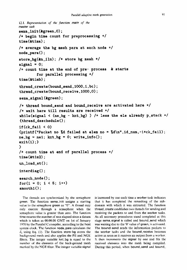
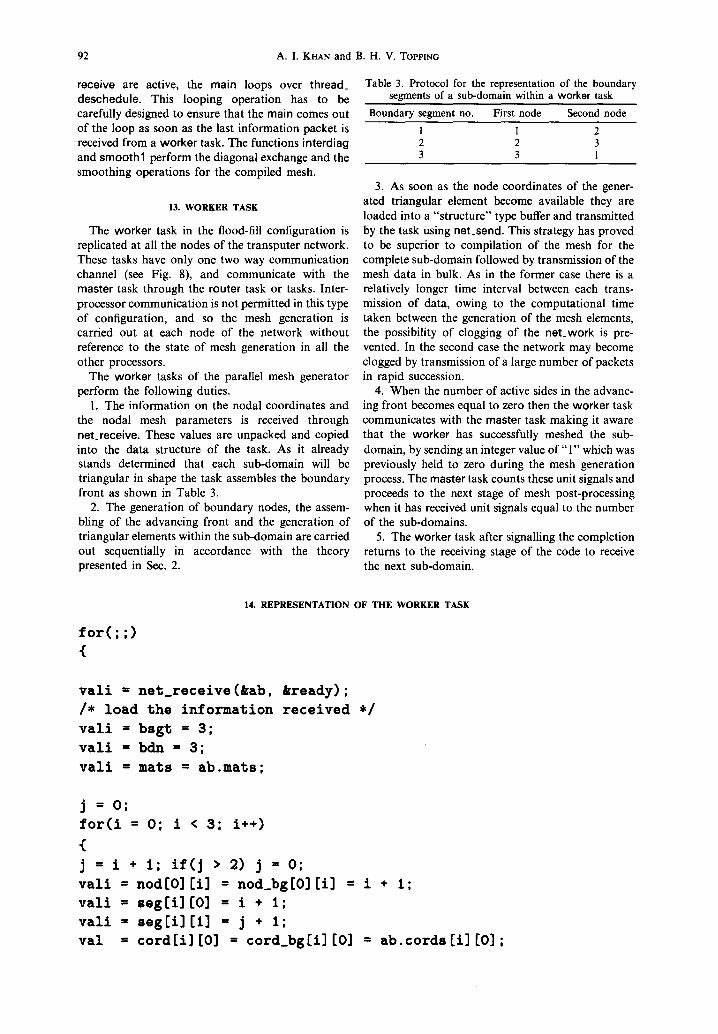
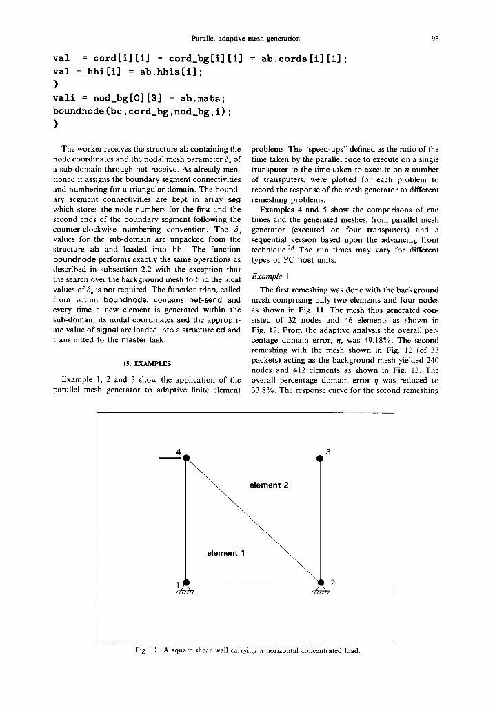
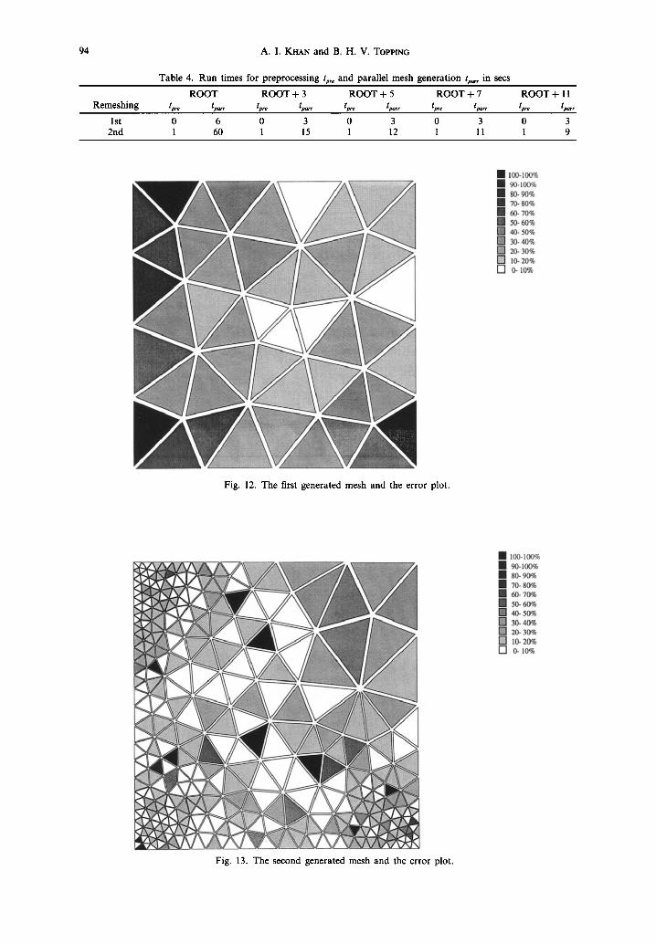
The first remeshing was done with the background mesh comprising only two elements and four nodes as shown in Fig. 11. The mesh thus generated con- sisted of 32 nodes and 46 elements as shown in Fig. 12. From the adaptive analysis the overall percentage domain error, q, was 49.18%. The second remeshing with the mesh shown in Fig. 12 (of 33 packets) acting as the background mesh yielded 240 nodes and 412 elements as shown in Fig. 13. The overall percentage domain error q was reduced to 33.8%. The response curve for the second remeshing

4 3

e lement 2

e lement 1

Fig. 11. A square shear wall carrying a horizontal concentrated load.

94 A. I. KHAN and B. H. V. TOPPING

Table 4. Run times for preprocessing tpr, and parallel mesh generation tp,, in sees

ROOT ROOT + 3 ROOT + 5 ROOT + 7 ROOT + 11 Remeshing tp, e t ~ , , t m t~r , tpr e t~r , tpr e t ~ , , tp, e t ~ , ,

1st 0 6 0 3 0 3 0 3 0 3 2nd 1 60 1 15 1 12 1 11 1 9

[ ] 100-100% [ ] 90-100% [ ] 80- 90% [ ] 70- 80% [ ] 60- 70% [ ] 50- 60% [ ] 40- 50% [ ] 30- 40% [ ] 20- 30% [ ] 10- 20% [ ] 0- 10%

Fig. 12. The first generated mesh and the error plot.

• 100-100% • 90-100% • 80- 90% • 70- 80% [ ] 60- 70% [] 50- 60% [] 40- 50% [] 30- 40% [] 20- 30% [] 10- 20% [] O- 10%

Fig. 13. The second generated mesh and the error plot.


33 PACKETS; 366 ELEMENTS

7 -

6-

5 -

3-

2-

I I I ~ I I I

2 4 6 8 10 12

Np(no.of processors)

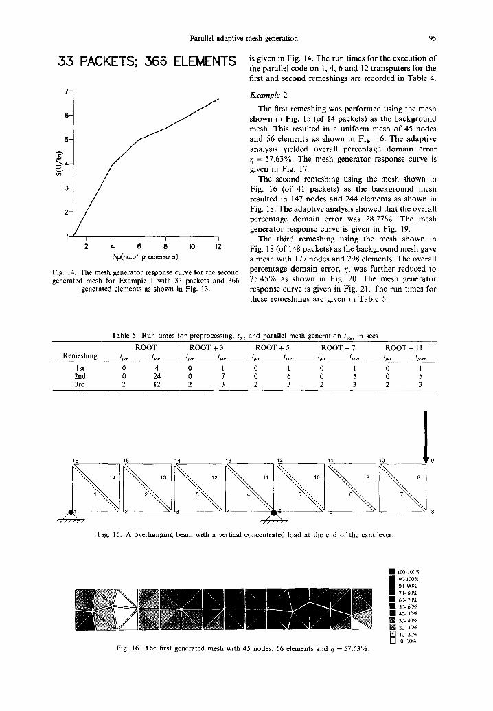
Fig. 14. The mesh generator response curve for the second generated mesh for Example 1 with 33 packets and 366

generated elements as shown in Fig. 13.

is given in Fig. 14. The run times for the execution of the parallel code on 1, 4, 6 and 12 transputers for the first and second remeshings are recorded in Table 4.

E x a m p l e 2

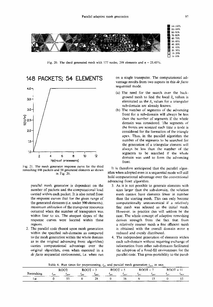
The first remeshing was performed using the mesh shown in Fig. 15 (of 14 packets) as the background mesh. This resulted in a uniform mesh of 45 nodes and 56 elements as shown in Fig. 16. The adaptive analysis yielded overall percentage domain error t / = 57.63%. The mesh generator response curve is given in Fig. 17.

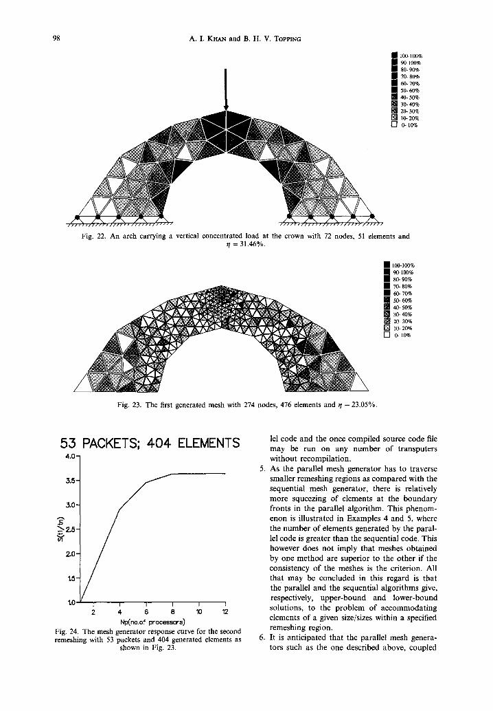
The second remeshing using the mesh shown in Fig. 16 (of 41 packets) as the background mesh resulted in 147 nodes and 244 elements as shown in Fig. 18. The adaptive analysis showed that the overall percentage domain error was 28.77%. The mesh generator response curve is given in Fig. 19.

The third remeshing using the mesh shown in Fig. 18 (of 148 packets) as the background mesh gave a mesh with 177 nodes and 298 elements. The overall percentage domain error, t/, was further reduced to 25.45% as shown in Fig. 20. The mesh generator response curve is given in Fig. 21. The run times for these remeshings are given in Table 5.

Table 5. Run times for preprocessing, tpr e and parallel mesh generation tpa,r in secs

ROOT ROOT + 3 ROOT + 5 ROOT + 7 ROOT + 11 Remeshing tpr e tparr tpr e lparr lpr e tparr Ipr e lparr lpr e tparr

1st 0 4 0 1 0 1 0 1 0 1 2nd 0 24 0 7 0 6 0 5 0 5 3rd 2 12 2 3 2 3 2 3 2 3

16 15 14 13 12 11 0 19

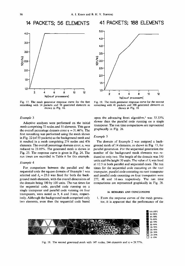
Fig. 15. A overhanging beam with a vertical concentrated load at the end of the cantilever.

uuuunnipj/! mN )NI)nmw

Fig. 16. The first generated mesh with 45 nodes, 56 elements and 1/ = 57.63%.

• 100-10(1% • 90-100% • 80- 90% [ ] 70- 80% [ ] 60- 70% • 50- 60% [ ] 40- 50% [ ] 30- 40% [ ] 20- 30% [ ] 10- 20% [ ] 0- 10%


14 PACKETS; 56 ELEMENTS 41 PACKETS; 188 ELEMENTS

4 .0 -

3.5-

3.0-

~ 2.5-

2.0-

10 I I I I I I

2 4 6 8 10 12 N p ( n o . o f processors)

Fig. 17. The mesh generator response curve for the first remeshing with 14 packets and 56 generated elements as

shown in Fig. 16.

5.0-

4 .5-

4.0-

3.5-

~ 3.0- ol

2.5-

Z 0 -

"1.5-

1.0 i l J J J J 2 4 6 8 10 12

N p ( n o . o f p r o c e s s o r s )

Fig. 19. The mesh generator response curve for the second remeshing with 41 packets and 188 generated elements as

shown in Fig. 18.

Example 3

Adaptive analyses were performed on the initial mesh comprising 72 nodes and 51 elements. This gave the overall percentage domain error r /= 31.46%. The first remeshing was performed using the mesh shown in Fig. 22 (of 53 packets) as the background mesh and it resulted in a mesh comprising 274 nodes and 476 elements. The overall percentage domain error, q, was reduced to 23.05%. The generated mesh is shown in Fig. 23. The response curve is given in Fig. 24. The run times are recorded in Table 6 for this example.

Example 4

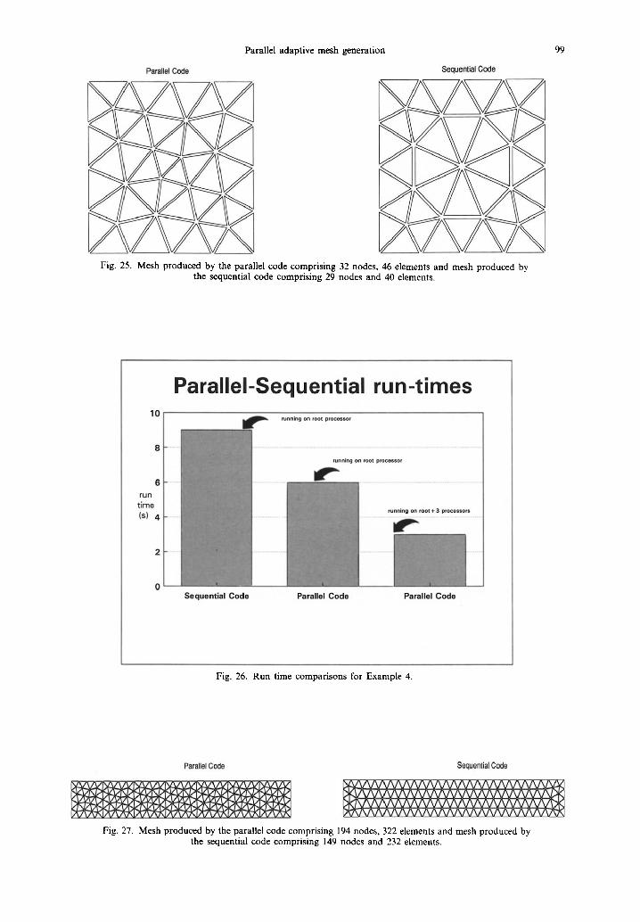
For comparison between the parallel and the sequential code the square domain of Example 1 was selected and 6, = 25.0 was fixed for both the background mesh elements, with the overall dimensions of the domain being 100 by 100 units. The run times for the sequential code, parallel code running on a single transputer and parallel code running on four transputers, were noted as 9, 6 and 3 secs, respectively. Although the background mesh comprised only two elements, even then the sequential code based

upon the advancing front algorithm, 2 was 33.33% slower than the parallel code running on a single transputer. The run time comparisons are represented graphically in Fig. 26.

Example 5

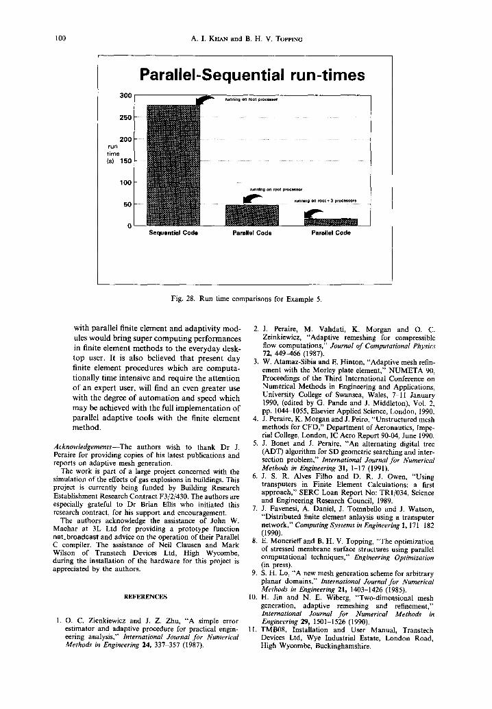
The domain of Example 2 was assigned a background mesh of 14 elements, as shown in Fig. 15, for parallel generation. For the sequential generation the number of the background mesh elements was reduced to only two. The length of the domain was 350 units and the height 50 units. The value of 6 i was fixed at 12.5 in both parallel and sequential cases. The run times for the sequential code executing on the root transputer, parallel code executing on root transputer and parallel code executing on four transputers were 277, 48 and 16secs respectively. The run time comparisons are represented graphically in Fig. 28.

16. REMARKS AND CONCLUSIONS

1. From the response curves of the mesh generator, it is apparent that the performance of the

m Fig. 18. The second generated mesh with 147 nodes, 244 elements and r/= 28.77%.

[ ] 100-100% [ ] 90-100% [ ] 80- 90% [ ] 70- 80% [ ] 60- 70% [ ] 50-60% [ ] 40- 50% [ ] 30- 40% [ ] 20- 30% [] lo- zo% [ ] 0- 10%


Fig. 20. The third generated mesh with 177 nodes, 298 elements and r/= 25.45%.

[ ] i00-100% [ ] 90-100% [ ] 80- 90% [ ] 70- 80% [ ] 60- 70% [ ] 50- 60% [ ] 40- 50% [ ] 30- 40% [ ] 20- 30% [ ] 10- 20% [ ] 0- 10%

148 PACKETS; 54 ELEMENTS

4°0 -

3 . 5 -

3 . 0 -

2.5- v ttl

Z 0 -

1 . 5 -

1.0 I I J I ~ J

2 4 6 8 10 12 Nt:~no.of processors)

Fig. 21. The mesh generator response curve for the third remeshing 148 packets and 54 generated elements as shown

in Fig. 20.

parallel mesh generator is dependent on the number of packets and the computational load carried within each packet. It is also noted from the response curves that for the given range of the generated elements (i.e. under 500 elements), maximum utilization of the transputer resources occurred when the number of transputers was within four to six. The steepest slopes of the response curves were located within these regions.

2. The parallel code (based upon mesh generation within the specified sub-domains as compared to the mesh generation within the whole domain as in the original advancing front algorithm) carries computational advantage over the original algorithm, even when executed in a de f a c t o sequential environment, i.e. when run

on a single transputer. The computational advantage results from two aspects in this de f a c t o sequential mode.

(a) The need for the search over the background mesh to find the local 6, values is eliminated as the 6, values for a triangular sub-domain are already known.

(b) The number of segments of the advancing front for a sub-domain will always be less than the number of segments if the whole domain was considered. The segments of the fronts are scanned each time a node is considered for the formation of the triangle apex. Thus, in the parallel algorithm the number of the segments to be searched for the generation of a triangular element will always be less than the number of the segments to be searched if the whole domain was used to form the advancing front.

It is therefore anticipated that the parallel algorithm when adopted even in a sequential mode will still hold computational advantage over the conventional advancing front algorithm.

3. As it is not possible to generate elements with sizes larger than the sub-domain, the solution mesh cannot have elements fewer in number than the starting mesh. This can only become computationally uneconomical if a relatively fine mesh was selected as the initial mesh. However, in practice this will seldom be the case. The whole concept of adaptive remeshing derives strength from the fact that from a relatively coarser mesh a fine efficient mesh is obtained with the overall domain error r/ reduced and evenly distributed.

4. The independent generation of elements within each sub-domain without requiring exchange of information from other sub-domains facilitated the adoption of a flood-fill environment tbr the parallel code. This gives portability to the paral-

Table 6. Run times for preprocessing, tpr e and parallel mesh generation tear, in sees

ROOT ROOT + 3 ROOT + 5 ROOT + 7 ROOT + 11 Remeshing tp,~ t ~ tp,~ lparr t m tp~ let e lparr lpr e lparr

1st 0 53 0 28 0 16 0 15 0 15

98 A. I. KHAN and B. H. V. TOPPING

[] 100-100% [] 90-100% [] 80- 90% [] 70- 80% [] ~ 70% [ ] 50- 60% [ ] 40- 50% [ ] 30- 40% [ ] 20- 30% [ ] 10- 20% [ ] 0- 10%

Fig. 22. An arch carrying a vertical concentrated load at the crown with 72 nodes, 51 elements and ~/= 31.46%.

• I00-100% • 90-i00 • • • 60- 0 [] 0-60 [ ] 40- 50% [ ] 30- 40% [ ] 20- 30% [ ] 10- 20% [ ] 0- 10%

Fig. 23. The first generated mesh with 274 nodes, 476 elements and ~/= 23.05%.

53 PACKETS; 4-04. ELEMENTS 4-.0-

3 .5-

,:3.0-

II1

2.0-

tS-

tO I I I I I l 2 4 6 8 10 12

Nt:~no.of processors) Fig. 24. The mesh generator response curve for the second remeshing with 53 packets and 404 generated elements as

shown in Fig. 23.

lel code and the once compiled source code file may be run on any number of transputers without recompilation.

5. As the parallel mesh generator has to traverse smaller remeshing regions as compared with the sequential mesh generator, there is relatively more squeezing of elements at the boundary fronts in the parallel algorithm. This phenom- enon is illustrated in Examples 4 and 5, where the number of elements generated by the parallel code is greater than the sequential code. This however does not imply that meshes obtained by one method are superior to the other if the consistency of the meshes is the criterion. All that may be concluded in this regard is that the parallel and the sequential algorithms give, respectively, upper-bound and lower-bound solutions, to the problem of accommodating elements of a given size/sizes within a specified remeshing region.

6. It is anticipated that the parallel mesh genera- tors such as the one described above, coupled


Parallel Code

d%ZZ)

Sequential Code

Fig. 25. Mesh produced by the parallel code comprising 32 nodes, 46 elements and mesh produced by the sequential code comprising 29 nodes and 40 elements.

Parallel-Sequential run-times o mnnlng on root proc~sor

running on root processor

tim (s)

0 Sequent ia l C o d e Paral lel C o d e Paral lel C o d e

Fig. 26. Run time comparisons for Example 4.

Parallel Code Sequential Code

Fig. 27. Mesh produced by the parallel code comprising 194 nodes, 322 elements and mesh produced by the sequential code comprising 149 nodes and 232 elements.

100 A. I . KHAN and B. H. V. TOPPING

300

250

20O r u n

time (s) 150

100

50

0

Parallel-Sequential run-times

Sequential Code Parallel Code Parallel Code

Fig. 28. Run time comparisons for Example 5.

with parallel finite element and adaptivity modules would bring super computing performances in finite element methods to the everyday desk- top user. It is also believed that present day finite element procedures which are computationally time intensive and require the attention of an expert user, will find an even greater use with the degree of automat ion and speed which may be achieved with the full implementation of parallel adaptive tools with the finite element method.

Acknowledgements--The authors wish to thank Dr J. Peraire for providing copies of his latest publications and reports on adaptive mesh generation.

The work is part of a large project concerned with the simulation of the effects of gas explosions in buildings. This project is currently being funded by Building Research Establishment Research Contract F3/2/430. The authors are especially grateful to Dr Brian Ellis who initiated this research contract, for his support and encouragement.

The authors acknowledge the assistance of John W. Machar at 3L Ltd for providing a prototype function net_broadcast and advice on the operation of their Parallel C compiler. The assistance of Neil Clausen and Mark Wilson of Transtech Devices Ltd, High Wycombe, during the installation of the hardware for this project is appreciated by the authors.

REFERENCES

1. O. C. Zienkiewicz and J, Z. Zhu, "A simple error estimator and adaptive procedure for practical engineering analysis," International Journal for Numerical Methods in Engineering 24, 337 357 (1987).

2. J. Peraire, M. Vahdati, K. Morgan and O. C. Zeinkiewicz, "Adaptive remeshing for compressible flow computations," Journal of Computational Physics 72, 449466 (1987).

3. W. Atamaz-Sibia and E. Hinton, "Adaptive mesh refinement with the Morley plate element," NUMETA 90, Proceedings of the Third International Conference on Numerical Methods in Engineering and Applications, University College of Swansea, Wales, 7-11 January 1990, (edited by G. Pande and J. Middleton), Vol. 2, pp. 1044-1055, Elsevier Applied Science, London, 1990.

4. J. Peraire, K. Morgan and J. Peiro, "Unstructured mesh methods for CFD," Department of Aeronautics, Impe- rial College, London, IC Aero Report 90-04, June 1990.

5. J. Bonet and J. Peraire, "An alternating digital tree (ADT) algorithm for SD geometric searching and inter- section problem," International Journal for Numerical Methods in Engineering 31, 1-17 (1991).

6. J. S. R. Alves Filho and D. R. J. Owen, "Using transputers in Finite Element Calculations: a first approach," SERC Loan Report No: TR1/034, Science and Engineering Research Council, 1989.

7. J. Favenesi, A. Daniel, J. Tomnbello and J. Watson, "Distributed finite element anlaysis using a transputer network," Computing Systems in Engineering 1, 171-182 (1990).

8. E. Moncrieff and B. H. V. Topping, "The optimization of stressed membrane surface structures using parallel computational techniques," Engineering Optimization (in press).

9. S. H. Lo, "A new mesh generation scheme for arbitrary planar domains," International Journal for Numerical Methods in Engineering 21, 1403-1426 (1985).

10. H. Jin and N. E. Wiberg, "Two-dimensional mesh generation, adaptive remeshing and refinement," International Journal for Numerical Methods in Engineering 29, 1501-1526 (1990).

l l. TMB08, Installation and User Manual, Transtech Devices Ltd, Wye Industrial Estate, London Road, High Wycombe, Buckinghamshire.


12. TMBI2, Installation and User Manual, Transtech Devices Ltd, Wye Industrial Estate, London Road, High Wycombe, Buckinghamshire.

13. INMOS Limited, Transputer Reference Manual, Prentice-Hall, Hertfordshire, UK, 1988.

14. K. C. Bowler, R. D. Kenway, G. S. Pawley and D. Roweth, An Introduction to OCCAM 2 Program- ming," Chartwell-Bratt Ltd, Studentlitteratur, Lund, 199I.

15. "Parallel C user Guide (compiler version 2.1)", Reference Manual, 3L Ltd, Livingston, Scotland, 1989.

16. "Tbug User Guide", 3L Ltd, Livingston, Scotland, 1989.

17. A. S. Tanenbaum, "Operating Systems: Design and Implementation," Prentice-Hall, Englewood Cliffs, N J, 1987.

parallel adaptive mesh generation

Documents