Refining Receptive Field Estimates using Natural Images for Retinal Ganglion Cells

Philip Vance, Gautham P. Das, Dermot Kerr and Sonya A. Coleman

School of Computing and Intelligent Systems,University of Ulster at Magee,

Londonderry, N. Ireland.email: {p.vance, g.das, d.kerr, sa.coleman}@ulster.ac.uk

Thomas M. McGinnitySchool of Science and Technology

Nottingham Trent University,Nottingham, United Kingdom.

email: martin.mcginnity@ntu.ac.uk

Abstract—Determining the structure and size of a retinal ganglion cell’s receptive field is critically important when formulating a computational model to describe the relationship between stimulus and response. This is commonly achieved using a process of reverse correlation through stimulation of the retinal ganglion cell with artificial stimuli (for example bars or gratings) in a controlled environment. It has been argued however, that artificial stimuli are generally not complex enough to encapsulate the full complexity of a visual scene’s stimuli and thus any model formulated under these conditions can only be considered to emulate a subset of the biological model. In this paper, we present an investigation into the use of natural images to refine the size of the receptive fields, where their initial location and shape have been pre-determined through reverse correlation. We present findings that show the use of natural images to determine the receptive field size provides a significant improvement over the standard approach for determining the receptive field.

Keywords- receptive field; retinal ganglion cell; retina; vision system; natural images.

I. INTRODUCTION

Vision begins when light is projected onto the retina at the back of the eye. It filters down through a complex layered organisation of cells consisting of photoreceptors, horizontal cells, bipolar-cells, amacrine cells and finally retinal ganglion cells. The Retinal Ganglion Cell (RGC) is the last point of contact within the retina before information is transferred to the visual cortex for higher processing. This makes the retina an ideal biological system to model, as visual stimuli that impact on the brain’s signal processing may be controlled while physiological information can be recorded simultaneously from multiple ganglion cells through the use of a multi-electrode array [1].

Each RGC has a Receptive Field (RF) that is defined as the area of sensory space (photo-receptors), which when stimulated, elicits a response. In reality, the general shape of a RF is irregular [2] though it is commonly approximated to be either circular [3] or elliptical with a 2D Gaussian spatial profile [4][5].

Identifying a RF in terms of its shape, size and location is critical in retinal modelling, as it is the first step in formulating a model that describes the relationship between stimulus and response. Mapping the RF is commonly carried out using a technique known as reverse correlation [5]–[9]. This method determines the size, location and shape of the

RF by stimulating the retina with artificial stimuli and analysing the correlation between the stimulus and output response. For instance, in [3], spot, annulus, and grating patterns are used to determine the size and location of the receptive field while other techniques use spatio-temporal checkerboard data [10], [11].

The drawback of determining the receptive field in this way is that artificial stimuli are generally not complex enough to describe natural visual scenes [12]–[15]. As the RGC cells are accustomed to the natural environment, natural images may be a more effective source of stimulation for characterising the RF [12]. The use of natural images has arguably become more popular within the last decade and has been shown to emphasize responses that were not as noticeable when using artificial stimuli [12]. In other work, it has been demonstrated that RFs derived from natural image stimuli are more robust in generalising novel stimuli not used in their estimation [9], as compared to RFs derived from artificial checkerboard and sparsely structured short bars.

In this paper, we present an investigation into the use of natural images to refine the size of a receptive field where the initial location and shape have been pre-determined through reverse correlation. The work presented uses the method detailed in [13], which investigates the responses of RGCs, in terms of their centres and surrounds, to natural images within rabbit RGCs. Here, we apply this method to salamander retinas and measure its performance with the popular Linear-Nonlinear (LN) cascade approach. We report on the effect of the determined surround area and provide supporting quantitative evidence of the benefits of using natural images as opposed to artificial stimuli.

Section II provides an overview of the experimental procedure used for the physiological experiments for both the artificial and natural image presentations. The receptive field estimation following data collection is outlined in Section III with an overview of how the spatial size is determined for the centre and surround. Results stemming from the use of this method are presented in Section IV with a conclusion and future work in Section V.

II. PHYSIOLOGICAL EXPERIMENT OVERVIEW

Retinas were isolated from dark adapted adult axolotl tiger salamanders similar to the approach in [1][16], where the retina is cut in half, with each half placed, cell-side down,

onto a multi-electrode array to record cell activations in response to presentation of varying stimulus inputs. The stimulus was projected onto the isolated retina using a miniature display coupled with a lens that de-magnifies the image and focuses it onto the photoreceptor layer. Sampled at 10 KHz, the recorded spikes were sorted off-line and spike times were measured relative to the beginning of the stimulus presentation.

Both artificial and natural image stimulation were utilised in these experiments. The artificial stimuli consisted of spatially arranged checkerboard patterns with no spatial or temporal order. The stimulus display ran at 60Hz whilst each checkerboard was updated at half this rate (30Hz) meaning a new checkerboard pattern was presented at approximately 3313

ms intervals. The dataset contained a large set of non-

repeated stimuli (258,000 samples) that are suitable to ascertain characteristics, such as the Spike-Triggered Average (STA, see below) and to ensure that a sufficient number of varied stimuli are presented in order to evoke cell responses.

Natural image stimuli were obtained from the McGill Calibrated Colour Image Database, which includes a wide range of visual scenes, each with a resolution of 256 x 256 pixels. Three hundred images were selected and arranged in a pseudo-random sequence and presented to the retina for 200ms, with an inter-stimulus interval of 800ms to allow each cell to recover from the previous stimulus update. A total of 13 presentations per image were carried out, with the mean response (per image) used for further calculations in this work.

III. RECEPTIVE FIELD ESTIMATION

In all, recordings for 49 RGCs were considered for determining the size and location of the receptive field (RF) for each RGC. Of these, 5 were classified as ON type cells by examining the shape of their temporal profiles [8][17][18], whilst the remaining exhibited temporal profiles similar to OFF type cells. Typically, the standard approach to estimating the size, shape and location of the RF is carried out using artificial checkerboard stimuli through a process of reverse correlation which is unsuitable for use with natural images [13][15].

A. Receptive-Field Estimation using Checkerboard StimuliReverse correlation (also known as spike-triggered

averaging) is the process of determining how cell activation is elicited through the study of how a sensory neuron sums stimuli that it receives at different times. The retina is stimulated with the spatio-temporal checkerboard stimuli; cell activations are recorded and used to calculate the average stimulus preceding a spike known as the STA [8]. Singular Value Decomposition (SVD) is then used to isolate the spatial component of the STA across time [19]. The process of defining the centre, size and shape of the RF is then accomplished by fitting a two-dimensional Gaussian function to the separated spatial component.

B. Refining RF Estimation using Natural ImagesThe use of natural images to determine the size of the RF

is based on a technique detailed in [13] as the physiological experiments are similar to the experimental procedure outlined in Section II. Alternative methods involve data manipulation during the experimental procedure [9][14], which doesn’t align well with the presented approach. The aim is to utilise this approach to refine the predefined size of the 2D fitted Gaussian function. The method outlines a two-stage process that first determines the centre of the RF followed by the estimation of the surround with natural image stimuli.

1) Centre EstimationIn [13], centre estimation is performed through a series of

estimated centre sizes and their cross-correlation with the cell’s response. Here, a range of assumed centre sizes are projected while retaining the original shape of the 2D Gaussian fitted function.

Figure 1. Series of guessed centre sizes for the RF.

Figure 1 depicts this process where a small subsample of estimates is demonstrated. In this example, the white disc represents the estimated centre size whilst the grey disc (in respect to this work) represents the original determined size of the RF through the reverse correlation technique. The black disc relates to the actual surround size, which will be further explained in the next section. For each estimated centre size, the mean contrast is calculated as:

(1)

where M c is the mean intensity of the centre region and M gray is the mean intensity of the entire image. A cross-correlation coefficient for each centre size is determined by:

(2)

where C c and are the centre mean contrast for an individual image and mean of centre mean contrasts for all images respectively. A cell’s response to an image is denoted by r (which is the cell’s recorded neural response as defined

in the experimental setup, Section II) whilst is the mean of a cell’s response to all images. The cross-correlation coefficient essentially looks for a relationship between the centre mean contrast and the output response. As ON type cells respond to high contrast values [20] this coefficient should rise in proportion to the increase in the estimated centre size, until a point where the centre starts to be influenced by what should

be the beginning of the surround area that adds inhibition. Conversely, OFF type cells are influenced by low contrast. This defines an inverse relationship between the cross-correlation coefficient and centre mean contrast. Consequently, the resulting shape of the curves can be a U or inverted U shape for OFF and ON cells respectively as shown in Figure 2. The three coefficients plotted (for both OFF and ON type cells) represent the calculated values for the example three centre sizes estimated depicted in Figure 1. The estimated centre size is determined as the size that provides the maximum correlation for the ON-cell and maximum inverse correlation for the OFF-cell.

Figure 2. Example plot of the cross-correlation coefficient against the assumed centre size for both an a) ON and b) OFF cell.

2) Surround EstimationSimilarly to calculating the centre size, the approach to

calculating the surround size begins with a series of estimated surrounds in the form of annuluses. The first estimate begins at the edge of the calculated centre size from the previous example as shown in Figure 3 where the grey disc represents the newly defined centre size, the black disc represents the perceived surround size whilst the white annulus represents a positional estimate for the surround architecture.

Figure 3. Example of positional estimates for the surround architecture starting closest to the newly defined centre region (A) and expanding to the perceived outer region (C).

The surround mean contrast is calculated as in Eq. with one amendment that replaces the mean centre intensity (M c¿with the surround mean intensity(M ¿¿ s )¿. Given that the response for a cell is predominantly attributed to the stimulation of the centre region [8][19][21], a different approach is required to determine the effect of each surround annulus. Computing the effect of each annulus requires that a selection of images is found that contain very similar centre mean contrast values. For this selection, it can be assumed that the variance in response, upon subtracting the mean, can be attributed to the surround. Fitting this response as a function of the surround mean contrast and taking the slope of the best fit line is considered to represent the effect of the annulus. Upon calculating the effect for several different annuluses, it is plotted and fitted against the position of the surround annulus. Figure 4 indicates the type of curves

evident for a well behaved ON type cell and OFF type cell, respectively.

Not all cells conform to this characteristic curve and in such cases, this technique in determining the size of the surround annulus cannot be performed with confidence. For cells that do conform, the first position that shows weak inhibition (A) determines where the surround begins. A further increase in inhibition is then perceived for every concurrent estimated annulus until it reaches a turning point (B) where maximum inhibition is evident. Inhibition to the cell’s response is then gradually decreased for further positional estimations until it reaches the point of providing no inhibition to the cell’s response (C).

Figure 4. Characteristic curve fitted through the estimated annulus positions for an a) ON type cell and b) OFF type cell. The size of the annulus is determined by the distance from A to C.

As the effect of the surround has no longer any contribution, this is considered the end of the surround. Thus, the size of the surround is determined by the distance from position A – C. Where there is a differential between the end of the centre region and the beginning of the surround (as happens in some cases), the stimuli in this area are not considered to be contributory to either the cell’s activation or inhibition and are ignored.

IV. RESULTS

To benchmark each model’s performance, a standard LN cascade model is implemented, which uses stimulus values from each approach in turn. The LN model is a popular method of estimating the output firing rate of a neuron by applying the input to a linear temporal filter followed by a static non-linear transformation [8][22]. For the results presented in this section, we perform a number of different experiments that first determine the effect of the surround (if any) followed by a comparison between the newly defined centres and the predefined centres (using reverse correlation) considering the effectiveness of the model fit. In the case of the predefined centres, a Gaussian smoothing function is also applied to the input stimulus, which accentuates the contrast levels within the visual scene [23] representing the processing that occurs between photo-receptors and RGCs. The specific parameters for this method are obtained through the reverse correlation technique thus they are dependent on the predefined centre size. As a result, this technique was not directly transferable to the natural image method.

A. Estimated CentresThe pre-defined size and shape is estimated as a 2D Gaussian distribution and given by:

(3)

where z is the 2D spatial coordinates, is the centre of the RF and is the covariance matrix that defines the RF [7]. Manipulating this function allowed scaling of the RF while retaining the centre and shape. For this study, RGCs close to the edge of the image whose predefined RF area extended past the 256 x 256 confines of the visual scene were ignored.

Figure 5 shows a subsample of the resulting curves for two OFF and ON type cells. We found that just over half of all cells conformed to this characteristic ‘U’ shape. Cells that did not exhibit this irregular bell shaped description of the effect of the centre were considered unclassifiable as the correct centre size could not be determined with certainty.

Figure 5. Subsample of characteristic curves for both ON and OFF type cells where the cross correlation coefficient is plotted vs. the assumed centre size for four different cells.

B. Estimated SurroundsFor the calculated centres of each cell considered, a

number of annuluses of defined widths were formed for the surround estimation. We found that in most cases, the surround extended far beyond what we had initially estimated with a good proportion of the expected sizes extending beyond the visual scene. An example curve fit (3rd order polynomial), shown for cell 43, is displayed in Figure 6 where the maximum positional estimation failed to cross the zero threshold again. In these cases, we extrapolated the point at which the surround ends by computing the roots of the fitted polynomial.

To illustrate the extent by which the surround occupies the visual scene, consider Figure 7 where both the centre and surround are indicated for both techniques. It is noticeable that the RF centre calculated via the reverse correlation method (red ellipse) is smaller than the defined centre using natural images. The surround (enclosed by blue ellipses) is quite large and expands close to the border of the visual scene. In many cases, the surround extended past the border and as a result, cells of this nature were excluded from the investigation.

C. Effect of SurroundIn the literature, the surround is considered to have a weak

to non-existent effect on a cell’s response [13][21]. Testing this theory for the axolotl tiger salamander RGC involved the use of the LN model with an input stimulus consisting of a combination of the centre values and varying contributions of the surround. We also evaluated the model with both the mean intensity and mean contrast values. Table 1 shows results for the RF presented in Figure 7 displaying the Root Mean Squared Error (RMSE) evaluation of the model fit. It is evident from these results that the RGC takes no contribution from the surround area given the proportional relationship between the RMSE and surround contribution, as is noted in the literature. Also apparent is the improvement in RMSE using the mean contrast values over the mean intensity. We found this to be the case for all cells evaluated with respect to the surround contribution.

Figure 6. Characteristic curve of the effect of the surround for cell 43.

Figure 7. Depiction of newly defined centre and surround for cell 43. Original spatial RF is enclosed with red ellipse whilst the newly defined surround is denoted with two blue ellipses.

TABLE 1. EFFECT OF SURROUND FOR CELL 43Surround

Contribution %

Mean Intensity

Mean Contrast

RMSE RMSE0 2.40 2.3720 2.41 2.3940 2.43 2.4160 2.45 2.41

D. Natural Image vs. Artificial StimuliGiven that the surround makes a very limited contribution

to the modelling process, only the calculated centres using the mean contrast values were used as a direct comparison to those RFs calculated through reverse correlation. In contrast to the results already shown for the example cell (cell 43), two cells that respond frequently to stimulus presentation are shown in Figure 8. Here, the difference is illustrated between the calculated and predefined centres of these two cells that were previously omitted due to the surround areas expanding past the limits of the visual scene.

Figure 8. Calculated centres for cells 7 (left) and 14 (right). Red ellipse represents original spatial RF that is almost double in size of their calculated counterparts.

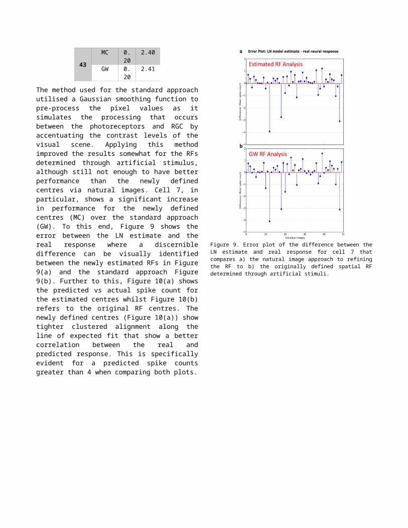
Encircled in red, the predefined RF in both cases is almost twice the size of the newly calculated centres via natural image stimulation. In Table 2, MC represents the stimulus associated with the mean contrast values determined through the natural image approach whilst GW denotes the Gaussian weighted pixels associated with RFs determined through reverse correlation using artificial stimulus. Using MC values of newly defined RFs demonstrates a considerable improvement in terms of both the R2 and RMSE compared with the standard approach (GW).

TABLE 2. RESULTS FOR LN ESTIMATES VS. REAL RESPONSE Cel

lMetho

dR2 RMS

E

7

MC 0.90

0.88

GW 0.80

1.23

14

MC 0.72

0.96

GW 0.68

1.04

41

MC 0.01

2.46

GW 0.00

2.58

43

MC 0.20

2.40

GW 0.20

2.41

The method used for the standard approach utilised a Gaussian smoothing function to pre-process the pixel values

as it simulates the processing that occurs between the photoreceptors and RGC by accentuating the contrast levels of the visual scene. Applying this method improved the results somewhat for the RFs determined through artificial stimulus, although still not enough to have better performance than the newly defined centres via natural images. Cell 7, in particular, shows a significant increase in performance for the newly defined centres (MC) over the standard approach (GW). To this end, Figure 9 shows the error between the LN estimate and the real response where a discernible difference can be visually identified between the newly estimated RFs in Figure 9(a) and the standard approach Figure 9(b). Further to this, Figure 10(a) shows the predicted vs actual spike count for the estimated centres whilst Figure 10(b) refers to the original RF centres. The newly defined centres (Figure 10(a)) show tighter clustered alignment along the line of expected fit that show a better correlation between the real and predicted response. This is specifically evident for a predicted spike counts greater than 4 when comparing both plots.

Figure 9. Error plot of the difference between the LN estimate and real response for cell 7 that compares a) the natural image approach to refining the RF to b) the originally defined spatial RF determined through artificial stimuli.

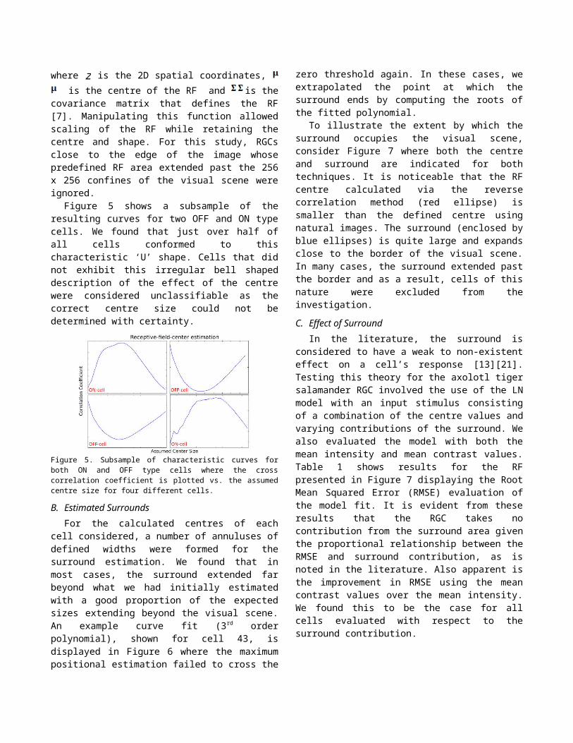
Figure 10. Plot showing the predicted vs. actual response for cell 7 that compares a) the natural image approach to refining the RF to b) the originally defined spatial RF determined through artificial stimuli.

V. CONCLUSION AND FUTURE WORK

In this work, an investigation into the use of natural images to refine the size of a RF has been presented, where their initial location and shape have been pre-estimated through reverse correlation. The precision of newly estimated centres is quantified by analysing a standard LN cascade model’s ability to describe the relationship between stimulus and response using the newly extracted stimulus as input. Results from this investigation provide supporting evidence to preliminary results in the literature that show the use of natural images, to improve the estimated size, provides a significant improvement over spatial profiles of RFs that have been derived entirely from artificial stimuli. An analysis of the effect of the calculated surround area was performed and found to have little to no contribution to the overall effect on the centre in terms of a cell’s response.

Due to the significant performance increase through modification of only the size of the RF, further study is merited to extend this investigation into the shape and location of the RF. In terms of the shape, recent studies have shown that focusing on sub-receptive fields (bipolar cell RFs [24]) provides a more accurate description of a cell’s response to stimulus by improving the ability to define with greater precision the actual shape of the RGC RFs and this will form the basis of our future research.

ACKNOWLEDGEMENTS

The research leading to these results has received funding from the European Union Seventh Framework Programme (FP7-ICT-2011.9.11) under grant number [600954] (“VISUALISE”). The experimental data contributing to this study have been supplied by the “Sensory Processing in the Retina” research group at the Department of Ophthalmology, University of Gӧttingen as part of the VISUALISE project.

REFERENCES

C. Fisher and W. A. Freiwald, “Whole-agent selectivitywithin the macaque face-processing system,” Proc. Natl.Acad. Sci. U.S.A., pp. 14717-14722, 2015.[3] W. F.Heine and C. L. Passaglia, “Spatial receptive field propertiesof rat retinal ganglion cells,” Visual neuroscience, vol. 28,no. 05, pp. 403–417, 2011.[4] J. W. Pillow et al.,“Spatio-temporal correlations and visual signalling in acomplete neuronal population,” Nature, vol. 454, no. 7207,pp. 995–9, 2008.[5] B. P. Olveczky, S. A. Baccus,and M. Meister, “Segregation of object and backgroundmotion in the retina.,” Nature, vol. 423, no. 6938, pp. 401–8, 2003.[6] D. Ringach and R. Shapley, “Reversecorrelation in neurophysiology,” Cognitive Science, vol. 28,no. 2, pp. 147–166, 2004.[7] T. Gollisch, “Estimatingreceptive fields in the presence of spike-time jitter.,”Network, vol. 17, no. 2, pp. 103–29, 2006.[8] E. J.Chichilnisky, “A simple white noise analysis of neuronallight responses.,” Network, vol. 12, no. 2, pp. 199–213,2001.[9] V. Talebi and C. L. Baker, “Natural versussynthetic stimuli for estimating receptive field models: acomparison of predictive robustness,” The Journal ofNeuroscience, vol. 32, no. 5, pp. 1560–1576, 2012.[10]D. Bölinger and T. Gollisch, “Closed-loop measurements ofiso-response stimuli reveal dynamic nonlinear stimulusintegration in the retina.,” Neuron, vol. 73, no. 2, pp. 333–46, 2012.[11] D. Takeshita and T. Gollisch, “Nonlinearspatial integration in the receptive field surround of retinalganglion cells,” The Journal of Neuroscience, vol. 34, no.22, pp. 7548–7561, 2014.[12] J. Touryan, G. Felsen,and Y. Dan, “Spatial structure of complex cell receptivefields measured with natural images.,” Neuron, vol. 45, no.5, pp. 781–91, 2005.[13] X. Cao, D. K. Merwine, and N.M. Grzywacz, “Dependence of Retinal Ganglion Cells’Responses to Natural Images on the Mean Contrasts of theReceptive-Field Center and Surround,” 2009.[14] J.Rapela, J. M. Mendel, and N. M. Grzywacz, “Estimatingnonlinear receptive fields from natural images.,” J Vis, vol.6, no. 4, pp. 441–74, 2006.[15] C. Kayser, K. P.Kӧrding, and P. Kӧnig, “Processing of complex stimuli andnatural scenes in the visual cortex,” Current opinion inneurobiology, vol. 14, no. 4, pp. 468–473, 2004.[16] J. K.Liu and T. Gollisch, “Spike-Triggered Covariance AnalysisReveals Phenomenological Diversity of Contrast Adaptationin the Retina,” PLoS Comput Biol, vol. 11, no. 7, p.e1004425, 2015.[17] R. Segev, J. Puchalla, and M. J.Berry, “Functional organization of ganglion cells in thesalamander retina.,” J. Neurophysiol., vol. 95, no. 4, pp.2277–92, 2006.[18] D. R. Cantrell, J. Cang, J. B.Troy, and X. Liu, “Non-centered spike-triggered covarianceanalysis reveals neurotrophin-3 as a developmentalregulator of receptive field properties of ON-OFF retinalganglion cells,” PLoS Comput Biol, vol. 6, no. 10, pp.e1000967–e1000967, 2010.[19] J. L. Gauthier et al.,“Receptive fields in primate retina are coordinated tosample visual space more uniformly,” PLoS biology, vol. 7,no. 4, p. 747, 2009.[20] D. H. Hubel, Eye, brain, and

[1] T. Gollisch and M. Meister, “Rapid neural coding inthe retina with relative spike latencies,” Science(80-. )., vol. 319, no. 5866, pp. 1108–1111, 2008.[2]C. Fisher and W. A. Freiwald, “Whole-agent selectivitywithin the macaque face-processing system,” Proc.Natl. Acad. Sci. U.S.A., pp. 14717-14722, 2015.[3]W. F. Heine and C. L. Passaglia, “Spatial receptivefield properties of rat retinal ganglion cells,” Visualneuroscience, vol. 28, no. 05, pp. 403–417, 2011.[4]J. W. Pillow et al., “Spatio-temporal correlations andvisual signalling in a complete neuronal population,”Nature, vol. 454, no. 7207, pp. 995–9, 2008.[5] B. P.Olveczky, S. A. Baccus, and M. Meister, “Segregationof object and background motion in the retina.,”Nature, vol. 423, no. 6938, pp. 401–8, 2003.[6] D.Ringach and R. Shapley, “Reverse correlation inneurophysiology,” Cognitive Science, vol. 28, no. 2,pp. 147–166, 2004.[7] T. Gollisch, “Estimatingreceptive fields in the presence of spike-time jitter.,”Network, vol. 17, no. 2, pp. 103–29, 2006.[8] E. J.Chichilnisky, “A simple white noise analysis ofneuronal light responses.,” Network, vol. 12, no. 2, pp.199–213, 2001.[9] V. Talebi and C. L. Baker,“Natural versus synthetic stimuli for estimatingreceptive field models: a comparison of predictiverobustness,” The Journal of Neuroscience, vol. 32, no.5, pp. 1560–1576, 2012.[10] D. Bölinger and T.Gollisch, “Closed-loop measurements of iso-responsestimuli reveal dynamic nonlinear stimulus integrationin the retina.,” Neuron, vol. 73, no. 2, pp. 333–46,2012.[11] D. Takeshita and T. Gollisch, “Nonlinearspatial integration in the receptive field surround ofretinal ganglion cells,” The Journal of Neuroscience,vol. 34, no. 22, pp. 7548–7561, 2014.[12] J.Touryan, G. Felsen, and Y. Dan, “Spatial structure ofcomplex cell receptive fields measured with naturalimages.,” Neuron, vol. 45, no. 5, pp. 781–91, 2005.[13]X. Cao, D. K. Merwine, and N. M. Grzywacz,“Dependence of Retinal Ganglion Cells’ Responses toNatural Images on the Mean Contrasts of theReceptive-Field Center and Surround,” 2009.[14]J. Rapela, J. M. Mendel, and N. M. Grzywacz,“Estimating nonlinear receptive fields from naturalimages.,” J Vis, vol. 6, no. 4, pp. 441–74, 2006.[15]C. Kayser, K. P. Kӧrding, and P. Kӧnig, “Processing ofcomplex stimuli and natural scenes in the visualcortex,” Current opinion in neurobiology, vol. 14, no.4, pp. 468–473, 2004.[16] J. K. Liu and T.Gollisch, “Spike-Triggered Covariance AnalysisReveals Phenomenological Diversity of ContrastAdaptation in the Retina,” PLoS Comput Biol, vol. 11,no. 7, p. e1004425, 2015.[17] R. Segev, J. Puchalla,and M. J. Berry, “Functional organization of ganglioncells in the salamander retina.,” J. Neurophysiol., vol.95, no. 4, pp. 2277–92, 2006.[18] D. R. Cantrell,J. Cang, J. B. Troy, and X. Liu, “Non-centered spike-

triggered covariance analysis reveals neurotrophin-3 asa developmental regulator of receptive field propertiesof ON-OFF retinal ganglion cells,” PLoS Comput Biol,vol. 6, no. 10, pp. e1000967–e1000967, 2010.[19]J. L. Gauthier et al., “Receptive fields in primate retinaare coordinated to sample visual space moreuniformly,” PLoS biology, vol. 7, no. 4, p. 747, 2009.[20]D. H. Hubel, Eye, brain, and vision, vol. 22.Scientific American Library New York, 1988.[21]D. K. Merwine, F. R. Amthor, and N. M. Grzywacz,“Interaction between center and surround in rabbitretinal ganglion cells,” Journal of Neurophysiology,vol. 73, no. 4, pp. 1547–1567, 1995.[22] S.Ostojic and N. Brunel, “From spiking neuron models tolinear-nonlinear models,” PLoS Comput. Biol, vol. 7,no. 1, p. e1001056, 2011.[23] D. Kerr, T. McGinnity,S. Coleman, and M. Clogenson, “A biologicallyinspired spiking model of visual processing for imagefeature detection,” Neurocomputing, vol. 158, pp. 268–280, 2015.[24] G. W. Schwartz et al., “Thespatial structure of a nonlinear receptive field,” Nat.Neurosci., vol. 15, no. 11, pp. 1572–80, 2012.