1

Paper SAS1759-2015

Explaining the Past and Modeling the Future: An Overview of Econometrics Tools in SAS/ETS®

Kenneth Sanford and Mark Little, SAS Institute Inc.

ABSTRACT

The importance of econometrics in the analytics toolkit is growing every day. Econometric modeling helps uncover structural relationships in observational data. This paper highlights the many recent changes to the SAS/ETS® software portfolio that increase your power to explain the past and predict the future. Examples show how you can use Bayesian regression tools for price elasticity modeling, use state space models to gain insight from inconsistent time series, use panel data methods to help control for unobserved confounding effects, and much more.

INTRODUCTION

Econometric and time series methods are an important part of the analytics toolkit. This importance grows as business problems become more complex and data are collected with greater frequency. To address the business needs of SAS® users, SAS/ETS has continued to build tools for analytical users to extract value from these data. This paper highlights several enhancements to the SAS/ETS portfolio and shows how these tools can be applied to a specific business problem.

The first problem to be examined is the opportunity to use the most up-to-date information in the formulation of a forecast. An example also highlights the use of new, disparate data sources at differing time intervals to make predictions. It presents several new tools and features in SAS/ETS, including the SSM procedure and the SASEFRED interface engine. The second example highlights advancements in Bayesian analysis within the QLIM procedure. This example examines the use of an informative prior for estimating the own price elasticity for a revenue management example. The third example highlights the importance of panel data. Panel data methods are increasing in popularity as household or individual data are being collected at more than one time period. This final example shows how panel data methods can materially alter the sign and significance of estimates from an econometric model. In this example, which uses insurance data, the implication for policy evaluation is significant. For complete information about the latest features in the software, please refer to the SAS/ETS documentation.

NOWCASTING WITH MULTIFREQUENCY DATA IN THE SSM PROCEDURE

Time series data are observations that are collected on the same sampling unit over regular intervals. One of the most common uses of time series data is to extract information about underlying components, which might be regular seasonal or temporary cycles in the data. A time series might also be characterized by an underlying trend. Early detection of an underlying trend in the data might provide an early-warning system for catastrophic failure. This section shows how you can use the SSM procedure in SAS/ETS in the context of a multivariate time series to extract a common trend and to signal opportunities for intervention.

One application of early detection of an underlying trend is preventive maintenance of an economic system. This paper uses that trend, extracted from a multivariate time series data set, to offer moments for possible intervention. The main analytical tool in this study is a linear state space model that you estimate by using the Kalman filter and smoother (KFS). This paper uses a multivariate time series data set to look for an underlying trend. It also showcases another recent enhancement to SAS/ETS, the SASEFRED interface engine, which enables users to easily and dynamically extract data from the Federal Reserve Economic Data (FRED) repository and then use these data in a SAS program. The paper uses data from FRED to identify candidate time periods when “preventive maintenance” could be performed.

The Federal Reserve Bank of Philadelphia produces a well-known index of economic indicators called the Aruoba-Diebold-Scotti (ADS) business conditions index. This index is designed to incorporate high-frequency time series data, which might be recorded at different intervals, into one measure of aggregate

2

economic activity at a single moment in time. This type of “blended time frequency” index could be useful in the burgeoning area of forecasting called “nowcasting,” which uses nearly instantaneously recorded data to make forecasts. This example re-creates a slightly simplified version of the ADS by using data that are dynamically retrieved by the SASEFRED interface engine. Then, the example provides a framework for how to extract an underlying trend from those data and how to propose preventive maintenance for an economy.

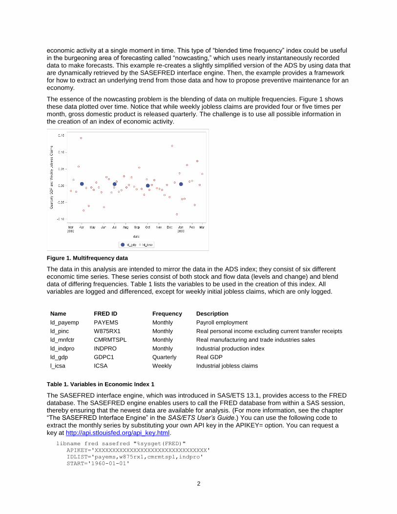
The essence of the nowcasting problem is the blending of data on multiple frequencies. Figure 1 shows these data plotted over time. Notice that while weekly jobless claims are provided four or five times per month, gross domestic product is released quarterly. The challenge is to use all possible information in the creation of an index of economic activity.

Figure 1. Multifrequency data

The data in this analysis are intended to mirror the data in the ADS index; they consist of six different economic time series. These series consist of both stock and flow data (levels and change) and blend data of differing frequencies. Table 1 lists the variables to be used in the creation of this index. All variables are logged and differenced, except for weekly initial jobless claims, which are only logged.

Name FRED ID Frequency Description

ld_payemp PAYEMS Monthly Payroll employment

ld_pinc W875RX1 Monthly Real personal income excluding current transfer receipts

ld_mnfctr CMRMTSPL Monthly Real manufacturing and trade industries sales

ld_indpro INDPRO Monthly Industrial production index

ld_gdp GDPC1 Quarterly Real GDP

l_icsa ICSA Weekly Industrial jobless claims

Table 1. Variables in Economic Index 1

The SASEFRED interface engine, which was introduced in SAS/ETS 13.1, provides access to the FRED database. The SASEFRED engine enables users to call the FRED database from within a SAS session, thereby ensuring that the newest data are available for analysis. (For more information, see the chapter “The SASEFRED Interface Engine” in the SAS/ETS User’s Guide.) You can use the following code to extract the monthly series by substituting your own API key in the APIKEY= option. You can request a key at http://api.stlouisfed.org/api_key.html.

libname fred sasefred "%sysget(FRED)"

APIKEY='XXXXXXXXXXXXXXXXXXXXXXXXXXXXXXXX'

IDLIST='payems,w875rx1,cmrmtspl,indpro'

START='1960-01-01'

3

END='2013-12-01'

FREQ='m';

Figure 2. Graphs of ADS Components

The series shown in Figure 2 can be considered as proxies for the health of the nation’s economy. Each series provides information about the health of the overall system, but each measure is imperfect because of other factors. It is reasonable to assume that each series contains a component that is common to all other series and that, when appropriately weighted, conveys information about the underlying health of the economic system. This example models this common component as an integrated random walk (𝑖𝑟𝑤_𝑡). The following observation equations formalize this system:

𝑦𝑖𝑡 = 𝑖𝑛𝑡𝑒𝑟𝑐𝑒𝑝𝑡𝑖 + 𝛽𝑖 ∗ 𝑖𝑟𝑤𝑡 + 𝜖𝑖𝑡 1 ≤ 𝑖 ≤ 5 𝑦6𝑡 = 𝛽6 ∗ 𝑖𝑟𝑤𝑡 + 𝜇𝑡 + 𝜖6𝑡

For 𝑦1𝑡 to 𝑦5𝑡 , the only other terms in the model are the respective intercepts, 𝑖𝑛𝑡𝑒𝑟𝑐𝑒𝑝𝑡𝑖, and the random

disturbances, 𝜖𝑖𝑡. Because 𝑦6𝑡 shows a pronounced nonstationary pattern, its model includes an

4

additional term, 𝜇𝑡, which is also modeled as an integrated random walk. For purposes of identification,

the initial condition for 𝑖𝑟𝑤𝑡 is assumed to be 0. For the same reason, 𝛽1 (the coefficient of 𝑖𝑟𝑤𝑡 in the model for 𝑦1𝑡) is assumed to be 1.

The underlying economic variables of the five time series, 𝑦1𝑡 to 𝑦5𝑡, are positively correlated with economic activity. For example, as payroll activity and economic activity both increase at the same time, only 𝑦6, the variable that measures initial jobless claims, is negatively correlated with economic activity. These correlations imply that, when 𝛽1is assumed to be 1, the estimates of 𝛽2, … , 𝛽5 are expected to be

positive and the estimate of 𝛽6 is expected to be negative. In the terminology of factor modeling, 𝑖𝑟𝑤𝑡 is

called a factor and 𝛽1, … , 𝛽6 are called the associated factor loadings.

USING THE SSM PROCEDURE TO SPECIFY THE MODEL

The following statements call the SSM procedure to estimate the factor loadings, which are shown in Table 2.

proc ssm data=econ opt(tech=activeset);

id date interval=day;

parms beta2-beta6; parms lv1-lv8;

avar = exp(lv7);

wnv1 = exp(lv1); wnv2 = exp(lv2); wnv3 = exp(lv3);

wnv4 = exp(lv4); wnv5 = exp(lv5); wnv6 = exp(lv6);

tvar = exp(lv8);

zero = 0;

/* --- start of model spec ----*/

state latent(2) t(g)=(1 1 0 1) cov(d)=(zero avar);

comp c1 = latent[1];

comp c2 = (beta2)*latent[1];

comp c3 = (beta3)*latent[1];

comp c4 = (beta4)*latent[1];

comp c5 = (beta5)*latent[1];

comp c6 = (beta6)*latent[1];

irregular w1 variance=wnv1; int1 = 1; /*define variance and intercept*/

model ld_payemp = int1 c1 w1; /*model for payroll employment*/

irregular w2 variance=wnv2; int2 = 1; /*define variance and intercept*/

model ld_pinc = int2 c2 w2; /*model for personal income*/

irregular w3 variance=wnv3; int3 = 1; /*define variance and intercept*/

model ld_mnfctr = int3 c3 w3; /*model for manufacturing sales*/

irregular w4 variance=wnv4; int4 = 1; /*define variance and intercept*/

model ld_indpro = int4 c4 w4; /*model for industrial production index*/

irregular w5 variance=wnv5; int5 = 1; /*define variance and intercept*/

model ld_gdp = int5 c5 w5; /*model for gdp*/

irregular w6 variance=wnv6 ; trend t_icsa(ll) levelvar=0 slopevar=tvar;

/*define variance and intercept*/

model l_icsa = c6 t_icsa w6; /*model for initial jobless claims*/

run;

The estimates in Table 2 are statistically significant, and their signs are economically consistent. These estimates correspond to the 𝛽𝑖 values in the model that is specified in the preceding statements, and they transmit information about economic activity to each series.

5

Parameter Estimate (Standard Error)

beta1 1 (.)

beta2 1.15 (0.1276)

beta3 1.96 (0.2390)

beta4 2.48 (0.1646)

beta5 3.27

(0.2653)

beta6 —96.42 (9.5909)

Table 2. Factor Loading Estimates

An important and valuable feature of the SSM procedure is its ability to do post-estimate processing from within the procedure. In addition to forecasting, post-estimate processing includes combining estimates and variables in various ways to produce calculations of interest. The following statements demonstrate these features and can be placed within the previous SSM procedure call:

/*code within PROC SSM for evaluating components*/

eval icsaPattern = c6 + t_icsa;

/*--index is a scaled version of the common factor--*/

eval Index = 1000*c1;

comp slope = latent[2];

eval IndexSlope = 1000*slope;

output out=forecast1 press pdv;

/*end post-estimate processing*/

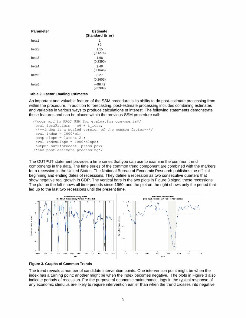
The OUTPUT statement provides a time series that you can use to examine the common trend components in the data. The time series of the common trend component are combined with the markers for a recession in the United States. The National Bureau of Economic Research publishes the official beginning and ending dates of recessions. They define a recession as two consecutive quarters that show negative real growth in GDP. The vertical bars in the two plots in Figure 3 signal these recessions. The plot on the left shows all time periods since 1960, and the plot on the right shows only the period that led up to the last two recessions until the present time.

Figure 3. Graphs of Common Trends

The trend reveals a number of candidate intervention points. One intervention point might be when the index has a turning point; another might be when the index becomes negative. The plots in Figure 3 also indicate periods of recession. For the purpose of economic maintenance, lags in the typical response of any economic stimulus are likely to require intervention earlier than when the trend crosses into negative

6

territory. By then it is too late. This is where expert judgment of the system is needed. This is just one type of analysis that you can do using the SSM procedure. To learn more about these methods, see the SAS/ETS 13.2 User’s Guide.

BAYESIAN ANALYSIS OF PRICE ELASTICITIES USING THE QLIM PROCEDURE

The number of rooms rented by a hotel, spending by loyalty-card customers, automobile purchases by households—these are just a few examples of variables that can best be described as “limited” variables. When limited (censored or truncated) variables are chosen as dependent variables, certain necessary assumptions of linear regression are violated. This section discusses the use of SAS/ETS tools to analyze data with a Bayesian approach. These options were recently added to the QLIM procedure.

PRICE ELASTICITY MODELING

Suppose you are a management analyst who is charged with estimating the price elasticity of for a product or service. More formally, the price elasticity of demand is

𝜖𝐷 =∆𝑄𝑢𝑎𝑛𝑡𝑖𝑡𝑦(𝑃𝑟𝑖𝑐𝑒) 𝑄𝑢𝑎𝑛𝑡𝑖𝑡𝑦(𝑃𝑟𝑖𝑐𝑒)⁄

∆𝑃𝑟𝑖𝑐𝑒 𝑃𝑟𝑖𝑐𝑒⁄

where Quantity(Price) is the dependent variable in the regression of quantity on price of the product and Price is the price of the product. Based on this regression model, ordinary least squares (OLS) or some other method of estimation can provide consistent estimates of the price elasticity if the error in the regression is not correlated with included regressors and if the dependent variable is not censored. The problem for a hotelier (or for any analyst in a capacity-constrained industry) is far more complex. Specifically, the hotelier is limited by the number of rooms available. Therefore, the upper bound on the number of rooms violates the assumption of normality of the data and the assumptions of the classic normal regression model. This problem of a censored distribution is relatively minor when the data rarely reach the threshold. However, for goods whose capacity is highly constrained, such as tickets and hotel rooms, sellouts are fairly common. In these cases, the upper-censoring problem creates meaningful challenges for estimating the elasticity of demand.

BIAS DUE TO CENSORING: A REAL-DATA EXAMPLE

The following data were collected for four different hotel properties (A, B, C, D) over a period of one year: • price of booking • occupancy (the number of rooms booked) • occupancy rate (the overall occupancy percentage of the hotel) • date when occupancy occurred

The data were collected daily for one-night stays only, for the same type of room, and with each booking taking place relatively close to the guest’s arrival. It is important to recognize that the occupancy and the occupancy rate are inversely related (see Figure 2). The censored observations (in red) are determined by the 90% threshold of “OccupancyRatio.”

7

Figure 4. Occupancy versus Occupancy Rate and Occupancy versus Price for Property A Figure 4 shows that a higher occupancy rate is associated with fewer booked rooms. Although this behavior might look unusual, it is consistent with the type of room under analysis because one-night stays, booked relatively close to the arrival time, are the most likely to be affected by the overall availability of the hotel. The limited availability of one-night stays when the hotel is nearly full results in a form of right-censoring, where there is a higher chance of the observation being censored when the observed booking rate is low. You might think that this phenomenon is the result of a large number of group sales for this night.

BAYESIAN APPROACH TO ESTIMATING PRICE ELASTICITY

Complicating the dependent variable censoring is the presence of identification problems across a number of properties. Whether this results from lack of data or little variation in data, certain hotel properties exhibit price elasticities that do not follow economic theory. This section shows how to incorporate an informed hierarchical prior into the analysis to produce estimates that are consistent with economic theory. Up to this point, all the analysis has focused on hotels whose price elasticities perform in accordance with economic theory. You would expect a price response for each property to be qualitatively similar to that for other properties—that is, a negative price response, as economic theory suggests. However, a preliminary analysis shows contradictory results: price seems to have a positive effect on the number of booked rooms. This behavior is unusual and contradicts what you learned from other properties.

Table 3. Posterior Summary with a Noninformative Prior

What can you do to inject additional information into the estimation process? Often managerial expertise or past experiences provide an opportunity to enrich your analysis. In this case you can use past information from other hotel properties.

8

The QLIM procedure now supports this sort of analysis with the inclusion of a BAYES statement. In this case, you can estimate a Bayesian version of your censored regression by using the following code:

proc qlim data=propertyB;

model Occupancy = Price /censored(lb=0 ub=UpperBound);

bayes nmc=30000 nbi=10000;

prior Price ~ Normal(mean=-0.037, var=0.00018);

run;

The results of the analysis in Table 4 from this model show some evidence that the estimated elasticities are at least negative, which is consistent with economic theory. In addition, the QLIM procedure provides a rich set of diagnostic graphs and tables via SAS ODS. This is shown in Figure 5 below.

Table 4. Posterior Summaries for Informative Prior

Figure 5. Diagnostic Plots from the QLIM Procedure

New Bayesian estimation options in the QLIM procedure in SAS/ETS 12.1 enable you to use potentially informative priors to assist in estimating price effects. These methods let you use data in ways that were previously not possible. To learn more about these methods, see the SAS/ETS 13.2 User’s Guide.

PANEL DATA METHODS TO CONTROL FOR CONFOUNDING EFFECTS

Panel data (sometimes called longitudinal data) can be thought of as the joining of cross-sectional and time series data. These data allow you to control for the effect of factors that are not accounted for by simple cross-sectional regression models that ignore the time dimension. These factors, which are unobserved by the modeler, might bias regression coefficients if left ignored This section introduces the concept of panel data and shows how treating data as a panel in a regression context can materially change the interpretation of the marginal effects.

9

WHAT ARE PANEL DATA?

Panel data can be thought of as repeated measurements on the same dependent and independent variables for a given sampling unit. That sampling unit could be a person, a household, a business, or even a geographic region. Panel data have a very specific structure in that the repeated observations are usually in evenly spaced intervals, such as days, weeks, months, or years. Figure 6 shows a typical structure of a panel data set.

ID Time doctor visits insurance health

Household 1 2011

Household 1 2012

Household 2 2011

Household 2 2012

… …

Household N 2011

Household N 2012

Figure 6. Example Panel Data Structure

WHY ARE PANEL DATA USEFUL?

Panel data have several distinct advantages that models built from purely cross-sectional or purely time series data cannot provide. Most notably these models can help with:

new policy questions via a quasi-experimental approach

time invariant unobserved heterogeneity and omitted variable bias

From a quasi-experimental approach, panel data enable you to perform before-and-after testing. In a cross-sectional data environment, there is no time dimension to allow for this. In a pure time series environment, to identify an effect of an intervention, you must make the very strong assumption that nothing else changes over time. A panel data set you to relax both assumptions, as variation over time and across the sections is used to identify any marginal effect.

Panel data allow for the possibility of controlling for time-invariant unobserved heterogeneity. This means that you can treat the cross-sectional units as unique. Allowing for these differences helps the modeler control for how unobserved differences can be correlated with observed regressors, a common problem in econometric regression. These unobserved differences can lead to inconsistent estimates of parameters from these models.

APPLICATION OF PANEL DATA IN HEALTH ECONOMICS

This section examines the application of panel data in a model of health care utilization. The German Socioeconomic Panel Survey was conducted between 1984 and 1995. Among other variables, the survey followed the healthcare utilization of households. The survey also contains information about possible factors for the difference in healthcare utilization among persons, including self-reported health status and the type of health insurance that the individual has.

A model to explain healthcare utilization is proposed; its dependent variable is annual visits to the doctor. The number of annual visits is a function of certain characteristics, including the person’s age, sex, health status (self-reported), income, and a number of other controls. The main variables of interest are the type of insurance (public or private) and the presence or absence of private supplemental insurance.

10

Table 5 presents results from two separate regression models. In both cases it is assumed that the data are conditionally negatively binomial distributed. This model is estimated using the COUNTREG procedure. Table 5 shows a subset of the coefficients from the following PROC COUNTREG run:

proc countreg data=surve(where=(female=1));

model docvis= age--public addon /dist=negbin;

model docvis= age--public addon /dist=negbin errorcomp=fixed;

run;

Variable (females only) (1) Pooled Data

(2) Fixed Effects

Health Status (0=bad, 10=good) -0.21* -0.14*

(0.004) (.005)

….

Public Insurance 0.11* 0.03

(0.045) (0.05)

Supplemental Insurance -0.008 0.16*

(.078) (0.08)

Table 5. Coefficients from COUNTREG Procedure

Model 1 treats the data as independent in both the cross section and the time dimension as the data are pooled for estimation. For space considerations, only a subset of the coefficients are shown. You can see that the sign on the coefficient of health status is negative and significantly different from zero; this is consistent with theory. The estimated coefficient on supplemental insurance is counterintuitive. In essence, this variable measures the presence of additional insurance for the individual. Theory would suggest that the effect of additional insurance would be positive, because it would effectively lessen the explicit cost of a doctor visit. The estimate for this coefficient in Model 1 is perplexing.

To further examine this effect, explicitly consider the panel structure of these data. Each year, the decision must be made to purchase this supplemental insurance. For this reason, a fraction of the sample changes states each year, from having this insurance to not having it, or vice versa. These transitions create a sort of quasi-experimental structure that enable the researcher to evaluate doctor visits before and after the change in state, and compare the change in doctor visits for those cases to the change in visits of those not changing insurance coverage status. Model 2 gives the coefficients for the panel data model, estimated by a model that has person-specific fixed effects. This approach yields economically consistent and statistically significant effects for supplemental insurance. That is, supplemental insurance increases the number of doctor visits, all else equal.

There are several SAS/ETS procedures that enable you to work with panel data. In addition to the COUNTREG procedure, the PANEL procedure lets you estimate many linear panel models. To learn more about these methods, see the SAS/ETS 13.2 User’s Guide.

11

CONCLUSION

This paper introduces three of the most recent themes in SAS/ETS software development. First, it examines the use of real-time data in the creation of an index of economic activity. Using the SSM procedure, it shows how to extract a common time trend from data on multiple frequencies. The second example introduces the Bayesian simulation options within the QLIM procedure. Historical information about the estimates of parameters from different samples inform the analysis through a Bayesian prior. The third example highlights recent developments to procedures that work with panel or longitudinal data. This example shows how to use data on both time series and cross-section dimensions allows you to control for unobserved differences among individuals, and how that control can lead to consistent estimates of the parameters of interest. To learn more about these methods, see the SAS/ETS 13.2 User’s Guide.

REFERENCES

Macaro, Chvosta, Sanford, and Lemieux, (2013). “Estimating Price Elasticities with Censored Data Using SAS/ETS.” Proceedings of the SAS Global Forum 2013 Conference, SAS Institute Inc.

Sanford, (2014). “When Do You Schedule Preventive Maintenance? Multivariate Time Series Analysis in SAS/ETS” Proceedings of the SAS Global Forum 2014 Conference, SAS Institute Inc.

SAS Institute Inc. (2015). SAS/ETS 14.1 User’s Guide. Cary, NC: SAS Institute Inc.

CONTACT INFORMATION

Your comments and questions are valued and encouraged. Contact the authors:

Ken Sanford Mark Little SAS Institute SAS Institute Kenneth.Sanford@sas.com Mark.Little@sas.com

SAS and all other SAS Institute Inc. product or service names are registered trademarks or trademarks of SAS Institute Inc. in the USA and other countries. ® indicates USA registration.

Other brand and product names are trademarks of their respective companies.

12

BASIC INSTRUCTIONS

WRITING GUIDELINES

Trademarks and product names

To find correct SAS product names (including use of trademark symbols), see the Master Name List.

Use superscripted trademark symbols in the first use in title, first use in abstract, and in graphics, charts, figures, and slides.

Do not abbreviate product names. For example, you cannot use “EM” for SAS® Enterprise Miner™. After having introduced a SAS product name, you can occasionally omit “SAS” for certain products, provided that your editor agrees. For example, after you have introduced SAS® Simulation Studio, you can use occasionally use “Simulation Studio.”

Writing style

Use active voice. (Use passive voice only if the recipient of the action needs to be emphasized.)

Use second person and present tense as much as possible.

Run spellcheck, and fix errors in grammar and punctuation.

Citing references

All published work that is cited in your paper must be listed in the REFERENCES section.

If you include text or visuals that were written or developed by someone other than yourself, you must use the following guidelines to cite the sources:

If you use material that is copyrighted, you must mention that you have permission from the copyright holder or the publisher, who might also require you to include a copyright notice. For example: “Reprinted with permission of SAS Institute Inc. from SAS® Risk Dimensions®: Examples and Exercises. Copyright 2004. SAS Institute Inc.”

If you use information from a previously printed source from which you haven’t requested copyright permission, you must cite the source in parentheses after the paraphrased text. For example: “The minimum variance defines the distance between cluster (Ward 1984, p. 23)

TIPS FOR USING WORD

These instructions are written for MS Word 2007 and MS Word 2010. The steps are similar for MS Word 2003.

To select a paragraph style

1. Click the HOME tab. The most common styles in your document are displayed in the top right area of the Microsoft ribbon. If you don’t see a style you want, click the slanted down arrow at the bottom right corner of the Styles area, and scroll through the list. The main styles for this template are headings 1 through 4, PaperBody, and Caption. Avoid using other styles.

2. To change a paragraph style, click the paragraph to which you want to apply a style, and then click the style you want in the ribbon.

3. PaperBody (used for most text) is automatically applied when you press Enter at the end of any heading style or the Caption style.

To insert a caption

1. Click REFERENCES on the main Word menu.

2. Click Insert Caption.

3. Select the Label type you want.

4. Click OK.

13

To insert a cross-reference

1. Click REFERENCES on the main Word menu.

2. Click Cross-reference.

3. In the Reference type list box, select Heading, Figure, Table, Display, or Output.

4. For a heading:

a. In the For which heading list, select the heading you want.

b. From the Insert reference to list, select Heading text.

5. For a figure, table, display, or output:

a. In the For which caption list, select the caption you want.

b. From the Insert reference to list, select Only label and number.

To insert a graphic from a file

1. Click INSERT on the main Word menu.

2. Click Pictures.

3. In the Insert Picture dialog box, navigate to the file you want to insert.

4. When the name of the file you want to insert is displayed in the File name box, click Insert.