Exegeses on Linear Models

Paper presented to the S-PLUS User’s ConferenceWashington, DC, 8-9th October, 1998

W N VenablesThe University of Adelaide

May 13, 2000

Contents

1 Preliminaries and introduction 1

2 A view of regression models 2

2.1 Extending the model . . . . . . . . . . . . . . . . . . . . . . . . . . . . . . . . 3

2.2 Additive models . . . . . . . . . . . . . . . . . . . . . . . . . . . . . . . . . . . 4

3 Some simple examples 5

3.1 The Janka hardness data . . . . . . . . . . . . . . . . . . . . . . . . . . . . . . 5

3.2 An additive model that seems to work . . . . . . . . . . . . . . . . . . . . . . 9

4 Variance heterogeneity 9

5 The SAS factor 11

5.1 ‘Type III’ sums of squares . . . . . . . . . . . . . . . . . . . . . . . . . . . . . 12

5.2 An example: The rat genotype data . . . . . . . . . . . . . . . . . . . . . . . . 14

6 Enhancements 17

7 Mixed effects, multistratum models and variance components 18

7.1 An example: the petroleum data of Nilon H Prater . . . . . . . . . . . . . . . 20

A Data sets used 22

1 Preliminaries and introduction

An exegesis is a marginal note or footnote expanding on the text, particularly in ecclesi-astical contexts such as in canon law. Some non-ecclesiastical exegeses are quite famous,such as the one that says “I have found a truly remarkable proof of this assertion butthere is not sufficient space to write it down here”. Others deserve to be, such as thepencil annotation I once discovered in a very old book on the English monarchy in mycollege library. Beside the paragraph describing how Charles II departed this world andwas buried it continued the final sentence with “. . . and whose epitaph might have been‘Here lies a profligate, licentious, perfidious, lascivious old scoundrel!’”

1

There is an element of whimsy in the title, of course, with an oblique suggestion thatperhaps people take linear models a little too seriously these days. On the other hand,as Brian Ripley and I say in our joint book, linear models form the core of modern ap-plied statistical practice, so they are indeed rather important. In this talk I would liketo present a view of linear models that is in many ways the folklore of the subject, cer-tainly for some of the more experienced (probably meaning simply ‘older’) practitionersbut unfortunately is not presented often enough or clearly enough in the current crop oftextbooks or, more particularly, in the current slew of wordy software manuals.

In so doing I hope to make some side comments—exegeses—that I hope provoke peo-ple into a minor, largely personal re-examination of linear models and, more importantlyfor us here at this conference, of the software used to support the praxis of linear mod-els. If they prove controversial this perhaps will serve to get your minds into gear andyourselves engaged in fruitful, or perhaps heated dialogue, as befits one of these raregatherings where so many of us who know each other only at the ends of an email linkfinally get to see one another face to face - and slug it out.

2 A view of regression models

Let Y be a quantitative response variable, x1, x2, . . . , xp potential quantitative explanatoryvariables andZ a standard normal variate. A model that says almost nothing useful aboutthe situation, but which nevertheless cannot seriously be challenged is that

Y = f(x; Z) (1)

where f(�) is some unknown, hopefully tame function.

Using a standard normal to inject error into the dependency is not without serious loss ofgenerality since any continuous distribution can be obtained by transformation from it,that is

E = F�1f�(Z)g

is a random variable with distribution function F (�), assuming continuity.

Assuming a steady-as-she-goes context, we might try to replace (1) by a local approxima-tion we recognize will only apply in the neighbourhood of some point x0 in design space.There are many ways we might do this, but surely the first and most obvious one, at leastin this slowly varying universe we are assuming, is a first order Taylor series:

Y � f(x0; 0) +pX

i=1

f (i)(x0; 0)(xi � xi0) + f (p+i)(x0; 0)Z

or, in more conventional notation

Y � �0 +pX

i=1

�i(xi � xi0) + �Z (2)

2

It does seem to be the case that most multiple regression models are really only intendedto be local linear approximations to something more complex, and hence will have arather closely proscribed domain of validity.

There is a tendency to simplify (2) even further and bundle all constant parts with respectto covariates into the intercept term and write it as

Y = �?0 +

pXi=1

�ixi + �Z

which may well be formally the same model, but I argue that this is not a practice to berecommended. for several reasons. The first of these is that if the covariates xi are all, say,positive but in any case reasonably far from 0, the constant term is the value of the meanat a point x = 0 likely to be far outside the domain in which the model is intended toapply, and hence likely to mislead naive clients as we shall shortly see in an example.

There may also be good numerical reasons for anchoring the x�variables at an originsomewhere near the centre of the section of design space covered by observations, but Ido not wish to push this point too far.

2.1 Extending the model

Following the same simple Taylor series heuristic, if we wished to improve the linearapproximation, and hopefully extend the practical domain of validity, we might nextconsider two terms in the Taylor series expansion. This gives an approximating model ofthe form

Y = �0 +pP

i=1�i(xi � xi0) +

pPi=1

pPj=i

�ij(xi � xi0)(xj � xj0)+�� +

pPi=1

i(xi � xi0)�Z + ÆZ2

(3)

Of course there is no guarantee that the heuristic remains particularly cogent and at somepoint practical considerations and experience with the context have to take over, but itis worth considering what it is this simple idea is telling us to look for in extending thelinear model, namely

� curvature in the main effects (quadratic terms in one variable),

� linear � linear interactions (cross product terms in two variables),

� variance heterogeneity (terms in (xi � xi0)Z) and

� skewness (the term in Z2),

which are all very commonly encountered problems in real life linear modelling, oftenignored but sometimes modelled in a more structured and context dependent way.

3

2.2 Additive models

The so-called additive models of (Hastie and Tibshirani, 1990) extend the first order modelin a different way, namely to a form

Y = �0 +pX

i=1

gi(xi) + �Z

where gi(x) may be a term consuming several degrees-of-freedom, or even a smoothingspline or locally weighted regression function that has to be estimated by non-standardmethods, but typically (though not always) it involves only one covariate.

My first reaction when I saw this was that it makes the strong assumption of no inter-actions between variables, but relatively weak assumptions about the form of the maineffects. I can remember expressing this objection to Trevor Hastie at a conference in 1993.This was clearly not the first time this question had been raised since he was well andtruly ready for me and had many reasons why such a model was useful in practice. Thereasons included that such a modelling strategy isolated the effect of each variable and al-lowed the user to examine them separately to see which were important and which werenot.

Privately I remained not completely convinced, I must say. As a consultant I am veryfamiliar with the kind of user who simply cannot think in a way that admits interactionsbut who just wants to know “which of my variables are important, which are not andwhat are the important ones doing”. (This is very closely akin to the experimental designphilosophy that varies one variable, only, at a time—the sort of thing that factorial designprinciples should have put out of business for good but, sadly, has not, yet.) But GAMswere receiving such accolades at the time I did rather feel like the little boy trying tosuggest that the king had no clothes.

More recently, however, I was at an experimental design lecture in Oxford where thelecturer expressed precisely the same reservation about additive models as I had donesome years before, which made me feel rather more confident about the king’s state ofdress. (The speaker, by the way, was Sir David Cox.)

To put the contrary case, there are indeed practical situations where the possibility of im-portant interactions can safely be downgraded a priori and additive models can prove avery useful investigative or diagnostic device. Indeed I use them often this way myselfand encourage my students to do the same. But I do seriously suggest that the ques-tion of interactions must in some way—however informally or by appeal to context—beinvestigated and laid to rest first, since rather simple interactive models can sometimesbe approximated fairly well by complicated main-effect models, but these models do nothold up well in prediction and can be misleading if used for interpretation.

4

3 Some simple examples

3.1 The Janka hardness data

This is a favourite data set of mine with an Australian flavour to it, indeed an Australiantimber flavour, which was the (now politically rather unfashionable) business my latefather worked in all his life, and me off and on for most of my adolescence.

The dependent variable is the Janka hardness of timber samples, a structurally importantquantity known to be closely related to density, which is the only recorded determiningvariable. The data comes from an old but still fascinating textbook, ((Williams, 1959)),by E J Williams, who worked in the CSIRO Division of Forest Products before joiningMelbourne University. The full data set is given in Table 1 on page 23.

Williams simply used the data as an example where a quadratic regression was necessaryrather than simple linear regression. It was before the days when plots were commonlyshown in textbooks but fortunately complete data sets were. Had Williams done the plotI think he would have noticed some interesting features that these days would attractmuch greater attention.

A plot of the data is shown in Figure 1. Some of the general features I have suggested weshould anticipate happening with approximating linear models are almost apparent evenfrom this rather simple plot. The curvature in the main effect is more-or-less clear (whichis all that Williams was concerned with), but so is the variance heterogeneity, in this casean increase in variance as the density increases.

The quadratic regression can easily be shown to be an adequate degree of polynomialregression but a plot of residuals versus fitted values makes the variance heterogeneityand skewness starkly apparent, as shown in Figure 2

There is a plausible argument that much hangs on the value leading to the largest resid-ual, but even omitting this point the variance heterogeneity can be detected by standarddevices. Moreover some standard checks for outlying residuals fail to rule it out of courteven as it stands.

Box and Cox transformations are interesting with this data set, as it turns out you needsomething like a square root transformation to make the quadratic regression linear, butsomething close to a log transformation to make the variance stable and remove the skew-ness credibly.

With this cue John Nelder once suggested to me using a generalized linear model with asquare root link to make the linear predictor linear in density rather than quadratic, anda variance function proportional to the square of the mean:

� = (�0 + �1x)2; Var[Y ] / �2

which implies that the original observations have a gamma distribution. This modelworks remarkably well, giving deviance residuals uniform beyond suspicion and a fairly

5

500

1000

1500

2000

2500

3000

30 40 50 60 70

Density

Har

dnes

s

Figure 1: The Janka hardness of timber data. Source: Williams (1959)

-200

0

200

400

500 1000 1500 2000 2500 3000

Fitted values

Res

idua

ls

Figure 2: Residuals versus fitted values after a quadratic regression of Hardness on Den-sity in the Janka data.

6

simple expression for hardness in terms of density. Two features should be acknowl-edged, though

� The predictions from the gamma model are virtually identical to those obtainedby Williams using an ordinary quadratic regression. Where the more sophisticatedmodel does offer some advantages, though, is in assessing the errors of prediction.The less dense timbers have a much tighter error bound with the gamma model thanwith the normal, and the heavier timbers a wider one, as seems to be appropriate.

� The real loss of degrees of freedom for estimation is probably slightly larger than itappears, considering the amount of data data snooping that went into the modellingproposal, but that could be checked by some of the standard means, such as cross-validation, bootstrap validation or using a confirmatory sample if available.

One final important point will be made with this simple example. Look at the differencesbetween fitting the polynomial models, here taken up to degree 3 for illustration, in a zerocentred and a median centred form.

> jank.1 <- lm(Hardness ˜ Density + Densityˆ2, Janka)

> round(summary(jank.1)$coefficients, 2)Value Std. Error t value Pr(>|t|)

(Intercept) -118.01 334.97 -0.35 0.73Density 9.43 14.94 0.63 0.53

I(Densityˆ2) 0.51 0.16 3.25 0.00

> jank.1a <- update(jank.1, . ˜ . + Densityˆ3)> round(summary(jank.1a)$coefficients, 2)

Value Std. Error t value Pr(>|t|)(Intercept) -641.44 1235.65 -0.52 0.61

Density 46.86 86.30 0.54 0.59I(Densityˆ2) -0.33 1.91 -0.17 0.86I(Densityˆ3) 0.01 0.01 0.44 0.66

Figure 3: Fitting quadratic and cubic models for the Janka data in zero centred form

7

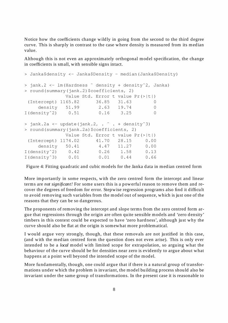
Notice how the coefficients change wildly in going from the second to the third degreecurve. This is sharply in contrast to the case where density is measured from its medianvalue.

Although this is not even an approximately orthogonal model specification, the changein coefficients is small, with sensible signs intact.

> Janka$density <- Janka$Density - median(Janka$Density)

> jank.2 <- lm(Hardness ˜ density + densityˆ2, Janka)> round(summary(jank.2)$coefficients, 2)

Value Std. Error t value Pr(>|t|)(Intercept) 1165.82 36.85 31.63 0

density 51.99 2.63 19.74 0I(densityˆ2) 0.51 0.16 3.25 0

> jank.2a <- update(jank.2, . ˜ . + densityˆ3)> round(summary(jank.2a)$coefficients, 2)

Value Std. Error t value Pr(>|t|)(Intercept) 1174.02 41.70 28.15 0.00

density 50.41 4.47 11.27 0.00I(densityˆ2) 0.42 0.26 1.58 0.13I(densityˆ3) 0.01 0.01 0.44 0.66

Figure 4: Fitting quadratic and cubic models for the Janka data in median centred form

More importantly in some respects, with the zero centred form the intercept and linearterms are not significant! For some users this is a powerful reason to remove them and re-cover the degrees of freedom for error. Stepwise regression programs also find it difficultto avoid removing such variables from the model out of sequence, which is just one of thereasons that they can be so dangerous.

The proponents of removing the intercept and slope terms from the zero centred form ar-gue that regressions through the origin are often quite sensible models and ‘zero density’timbers in this context could be expected to have ‘zero hardness’, although just why thecurve should also be flat at the origin is somewhat more problematical.

I would argue very strongly, though, that these removals are not justified in this case,(and with the median centred form the question does not even arise). This is only everintended to be a local model with limited scope for extrapolation, so arguing what thebehaviour of the curve should be for densities near zero is evidently to argue about whathappens at a point well beyond the intended scope of the model.

More fundamentally, though, one could argue that if there is a natural group of transfor-mations under which the problem is invariant, the model building process should also beinvariant under the same group of transformations. In the present case it is reasonable to

8

require that the model building process be invariant with respect to changes of locationand scale in the density. This immediately requires that as long as there is a term in thepolynomial model of degree k, no term of degree less than k should be considered forexclusion.

Under these conditions we say that the intercept and linear terms are marginal to thequadratic term, a concept guaranteed to generate controversy like no other in this area.

Marginality is also at the crux of another thorny issue in linear models, namely that ofType III sums of squares, to which I shall return below.

3.2 An additive model that seems to work

To show my even-handedness on the issue, I present below a textbook example whereadditive models do seem to offer a useful perspective on the data, but I have concealedmy attempts to resolve the question of interactions beforehand, which to my satisfactionled me to assume that in this case they could safely be ignored.

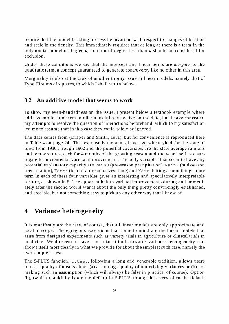
The data comes from (Draper and Smith, 1981), but for convenience is reproduced herein Table 4 on page 24. The response is the annual average wheat yield for the state ofIowa from 1930 through 1962 and the potential covariates are the state average rainfallsand temperatures, each for 4 months of the growing season and the year itself as a sur-rogate for incremental varietal improvements. The only variables that seem to have anypotential explanatory capacity are Rain0 (pre-season precipitation), Rain2 (mid-seasonprecipitation), Temp4 (temperature at harvest time) and Year . Fitting a smoothing splineterm in each of these four variables gives an interesting and speculatively interpretablepicture, as shown in 5. The apparent halt to varietal improvements during and immedi-ately after the second world war is about the only thing pretty convincingly established,and credible, but not something easy to pick up any other way that I know of.

4 Variance heterogeneity

It is manifestly not the case, of course, that all linear models are only approximate andlocal in scope. The egregious exceptions that come to mind are the linear models thatarise from designed experiments such as variety trials in agriculture or clinical trials inmedicine. We do seem to have a peculiar attitude towards variance heterogeneity thatshows itself most clearly in what we provide for about the simplest such case, namely thetwo sample t�test.

The S-PLUS function, t.test , following a long and venerable tradition, allows usersto test equality of means either (a) assuming equality of underlying variances or (b) notmaking such an assumption (which will always be false in practice, of course). Option(b), (which thankfully is not the default in S-PLUS, though it is very often the default

9

Year

s(Y

ear)

1930 1940 1950 1960

-20

-10

010

20

• •• •

•

• •

•

••

•

•• • •

•

••

•

• •

•

•

• ••

•• •

••

• •

Rain0

s(R

ain0

)

15 20 25

-20

-10

010

20

•

•

•

•

•

••

•

••

• •

•

••

•

•

•

•

••

•

•

•••

•

••

•

•

••

Rain2

s(R

ain2

)

2 4 6

-20

-10

010

20

• • • •

•

•

•

•

••

•

•

••

•

•

•

•

•

••

•

•

•••

•••

•

•

••

Temp4

s(T

emp4

)

68 70 72 74 76 78 80

-20

-10

010

20

••

••

•

•

•

••

•

•

••

••

•

•

•

•

•••

•

••

•

•••

•

•

••

Figure 5: Additive model components for the Iowa wheat yield data.

elsewhere) gives naive users a cosy feeling of protection that perhaps their test makessense even if the variances happen to come out wildly different.

What’s the matter with that?

For one thing, not so naive users wonder why such a fuss is made of equal variance in thetwo sample t�test but elsewhere it is a non-problem, it seems. In the three sample casethe only software provided is the one-way analysis of variance where equality of varianceis, it seems, silently dismissed as a non-issue.

The main problem I see with it, though, and I see it often, is that it leads users away

10

from the important considerations of the problem. Variance heterogeneity is an importantproblem in all linear models and it can be the vital issue. If two samples show largeand established differences of variance, this is usually much more important than anydifference of means. If one treatment gives a higher yield than another, this is often not ofmuch interest if it also has a much higher error variance causing it to be unreliable.

In a sense, the onus is on the user to investigate variance heterogeneity along with in-vestigating mean differences. This is often done by diagnostic methods such as we didin the Janka data. Providing things like the modified t�test that ‘can be used even if theassumption of equal variances is not met’ is only encouraging naive users to miss thewhole point. To be candid I am not sure if this problem can really be fixed by changingthe software—in the long run users are (often) adults and must be trusted not to do sillythings—but as an educator and a user I feel obliged to voice my concern at what I seehappening.

5 The SAS factor

Many more S-PLUS users than I had expected would be the case are in fact refugees fromthe SAS regime. Even some of the authors of the voluminous SAS documentation are nowwell-known names in the S-PLUS world and some, though very few it seems, continue toplay a fairly prominent role in both camps.

I have involuntarily used SPSS many years ago but I have never seriously used SAS. Toprepare this talk I thought I would have to look closely at the SAS documentation, at least,to see how other software systems treat linear models these days, and since SAS seemsto be to statistical computing what Microsoft is to personal computing, it had to be thelogical next place to look. The only documentation I had available ((SAS Institute Inc.,1990)) dated from 1990, but I think for my purposes that would be current enough.

It must be said that although it is often very waffly and occasionally rather patronisingthe documentation for SAS is at least comprehensive and very often statistically astute (ifI might be permitted a similarly patronising rejoinder!) My first and strongest impression,though, is that SAS attempts to provide all functionality for all occasions—programmingis such a delicate and exacting job there must be no scope for ordinary users to do it forthemselves.

The goal of providing all necessary statistical and data analysis functionality in the oneawkward and foolishly consistent framework is uncannily like Microsoft and, (one hopesand prays), ultimately futile, but in the meantime what happens is that the program de-fines the subject rather than the subject dictating what the program should do. SAS, itseems, has become the gold standard, the output of SAS programs the ultimate point ofreference for correct and appropriate statistical calculations and the SAS terminology israpidly taking over as standard terminology. This is very Microsoft-like indeed and veryworrying for anyone who cares about the profession.

11

Nowhere, it seems to me, is this SAS coup d’etat more evident than in the way Analysis ofVariance concepts are handled.

There is no essential distinction between linear models we happen to call Regression andthose we call Analysis of Variance models, but with the latter the feature that makes themsomewhat special is that the natural parametrisation leads to design matrices not of fullcolumn rank. This in turn gives rise to the important notion of estimability of linear func-tions of the parameters.

In a sense this notion is easy. The means of the observations themselves are the onlywell-defined functions of the parameters; any function is estimable if and only if it can bewritten as a linear function of the observation means, that is the coefficient vector mustbe in the row space of the design matrix.

Many programs overcome this minor obstacle by omitting parameters in such a way thatthose remaining are all estimable. S-PLUS does this when it uses the contr.treatmentcontrast matrices, but for other contrast matrices the original redundant parameters arereplaced by a smaller set of more complicated linear functions of them which are, usually,estimable.

The clear and unequivocal message is, though, that a linear function of the parametersis either estimable or it is not; there are no shades of grey, no half way houses and nosubtle distinctions. With this in mind, the title of Chapter 9 of the SAS/STAT manual isworrying: The Four Types of Estimable Functions. Closer inspection reveals that this notionis really a kind of transferred epithet, and there are really four types of hypotheses beingconsidered, another equally curious distinction being made without a difference.

One sentence bears quoting: “The four types of hypotheses available in GLM may notalways be sufficient for a statistician to perform all desired hypothesis tests, but theyshould suffice for the vast majority of analyses.” In other words, the distinctions beingmade are limitations on the program rather than differences of principle in the subject,but then, it seems, the program really is defining the subject.

5.1 ‘Type III’ sums of squares

I was profoundly disappointed when I saw that S-PLUS 4.5 now provides “Type III” sumsof squares as a routine option for the summary method for aov objects. I note that it is notyet available for multistratum models, although this has all the hallmarks of an oversight(that is, a bug) rather than common sense seeing the light of day. When the decision wasbeing taken of whether to include this feature, “because the FDA requires it” a few of mycolleagues and I were consulted and our reply was unhesitatingly a clear and unequivocal“No”, but it seems the FDA and SAS speak louder and we were clearly outvoted.

So what is the problem with Type III sums of squares that is worth making such a fussabout?

12

It’s difficult to resist the same sort of words we use to explain the phenomenon to secondyear students. In fact I will not resist.

In a two-factor experiment the factors A and B are said to have an interaction if the changein the response mean resulting from a change in levels for factor A, say, depends on whichlevel of factor B is applied.

If any change in level for factor A always produces the same change in the response meanregardless of the level of factor B, the same must be true for factor B as well, and the twofactors are said not to have an interaction, or to act additively.

If factors act additively their main effects are well defined and testing whether their maineffects are zero or not is a sensible and useful thing to do.

If there is an interaction between factors A and B, it is difficult to see why the maineffects for either factor can be of any interest, since to know what the effect of changingan A�level on the response will be depends on which B�level is in force.

More pointedly, when there is an interaction in force, a routine test of the main effectscan be shown to be testing an hypothesis that depends on the design of the experimentrather than on the parameters alone. To overcome this manifestly arbitrary aspect of thetesting procedure, Type III sums of squares arise from testing an hypothesis—equallyarbitrary—connected with the parameters that does not vary with the design.

To hark back to a previous idea, testing main effects in the presence of an interactionis a violation of the marginality principle. This is not a totally rigid principle, but in allcommon practical situations the sensible thing is to respect it. Just as there are situationswhere it does make sense to fit a regression line through the origin, though, or to constraina fitted quadratic curve to be flat at some specified point, there are some very specialoccasions where some clearly defined estimable function of the parameters that wouldqualify as a definition of main effect to be tested, even when there is an interaction inplace, but like the regression through the origin case, such instances are extremely rareand special.

Just as providing a switch in the two-sample t�test to cover unequal variances encour-ages users to think that the annoying problem of variance inhomogeneity is nailed downand can be ignored, providing a deceptive “Type III” sum of squares option in he Analysisof Variance summary encourages users to think that the annoying problem of interactionscan be ignored and the main effect question—the one that everyone understands, eventhough in the presence of interaction it makes little sense—can be safely settled withoutworrying about pesky interactions, at least to the FDA’s satisfaction, and what more couldanyone ever want?

There is even a class of user now days who sees the significance stars (which fortunatelyS-PLUS does not yet provide, for who knows how long?) rather like the gold stars mygrandson sometimes gets on his homework. Three solid gold stars on the main effectswill do very nicely, thank you, and if there are a few little stars here and there on theinteractions, so much the better!

13

5.2 An example: The rat genotype data

The non-problem that Type III sums of squares tries to solve only arises because it is sosimple to do silly things with orthogonal designs. In that case main effect sums of squaresare uniquely defined and order independent. Where there is any failure of orthogonality,though, it becomes clear that in testing hypotheses, as with everything else in statistics, itis your responsibility to know clearly what you mean and that the software is faithfullyenacting your intentions.

Henri Scheffe in his classic text on The Analysis of Variance (Scheffe, 1959), gives an ex-ample of a 4�4 double classification with unequal cell frequencies, though not wildly so,that will do to illustrate some of these points. For convenience the data set is reproducedhere in Table 2 on page 23.

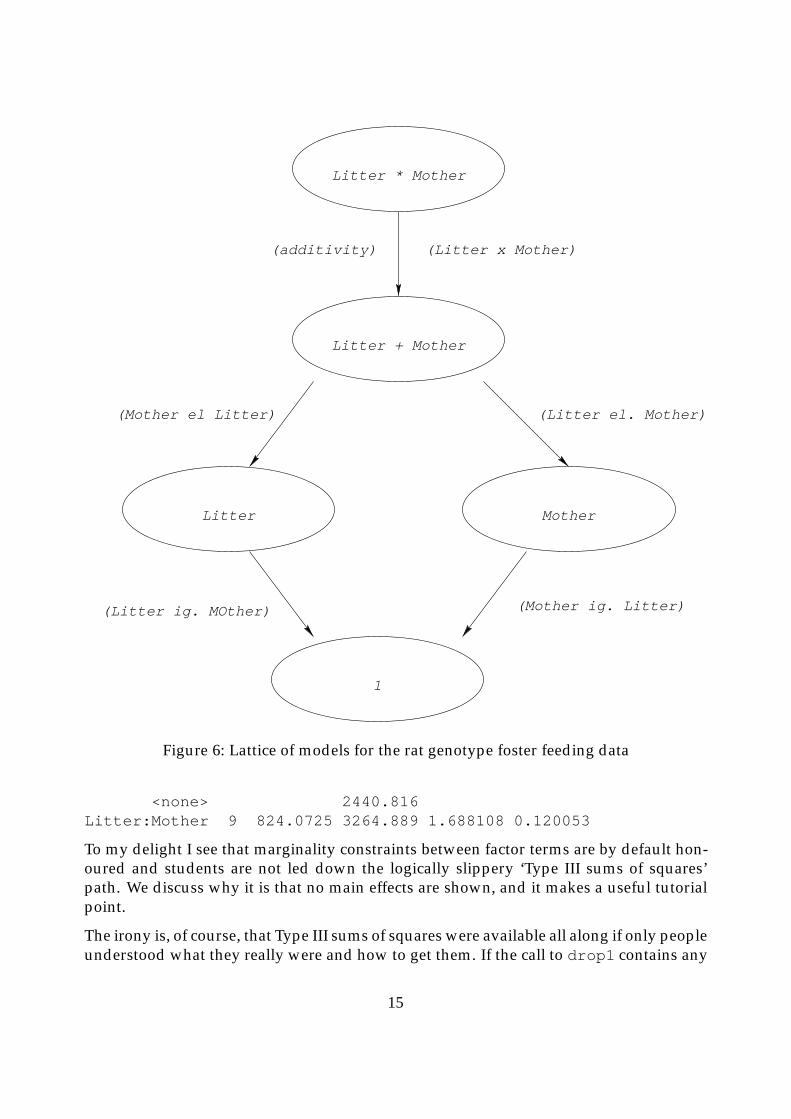
Litters of rats are separated from their natural mother and given to another female to raise.The two factors are the mother’s genotype and the litter’s genotype and the response isthe average weight gain per member of the litter. (There is an acknowledged componentof variance ignored in this, but as Scheffe says, it is likely to be very small.) The naturalmodels and the relations between them form a lattice that immediately makes clear whatany sum of squares means. This is shown in Figure 6.

Any path from the top of the lattice to the bottom gives sums of squares for testing eachmodel within the one immediately above it. Thus testing for Litters ignoring Mothers andfor Litters eliminating Mothers are both “main effect” sums of squares for Litters, but cor-respond to different tests of hypotheses, one assuming Mother’s genotype does not havean effect, the other allowing for the possibility that it may. For an orthogonal experi-ment, confusingly in a way, these sums of squares are numerically identical, even if thehypotheses they test are, conceptually at least, different.

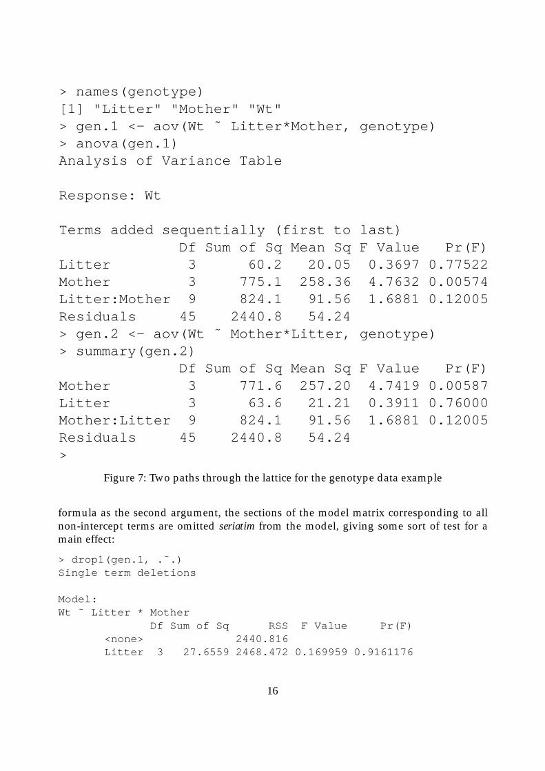
The difference here is only small, as we can easily check in Figure 7. Interactions appearignorable, so main effect tests start to make sense, and it becomes clear that the mother’sgenotype exerts a sizeable influence on average weight gain and litter’s genotype doesnot. This has to be checked graphically, of course, and when that step is taken it becomesclear that there is at least one large outlier and much hangs on whether that observationis correct or not.

When I use this example with my students, though, the first thing I ask them to do is tofit the full model and use drop1 to suggest the next step. Brilliantly, drop1 fingers theinteraction term, and the interaction term only:

> drop1(gen.1)Single term deletions

Model:Wt ˜ Litter * Mother

Df Sum of Sq RSS F Value Pr(F)

14

Litter * Mother

Litter + Mother

Litter Mother

1

(additivity)

(Litter ig. MOther) (Mother ig. Litter)

(Litter el. Mother)(Mother el Litter)

(Litter x Mother)

Figure 6: Lattice of models for the rat genotype foster feeding data

<none> 2440.816Litter:Mother 9 824.0725 3264.889 1.688108 0.120053

To my delight I see that marginality constraints between factor terms are by default hon-oured and students are not led down the logically slippery ‘Type III sums of squares’path. We discuss why it is that no main effects are shown, and it makes a useful tutorialpoint.

The irony is, of course, that Type III sums of squares were available all along if only peopleunderstood what they really were and how to get them. If the call to drop1 contains any

15

> names(genotype)[1] "Litter" "Mother" "Wt"> gen.1 <- aov(Wt ˜ Litter*Mother, genotype)> anova(gen.1)Analysis of Variance Table

Response: Wt

Terms added sequentially (first to last)Df Sum of Sq Mean Sq F Value Pr(F)

Litter 3 60.2 20.05 0.3697 0.77522Mother 3 775.1 258.36 4.7632 0.00574Litter:Mother 9 824.1 91.56 1.6881 0.12005Residuals 45 2440.8 54.24> gen.2 <- aov(Wt ˜ Mother*Litter, genotype)> summary(gen.2)

Df Sum of Sq Mean Sq F Value Pr(F)Mother 3 771.6 257.20 4.7419 0.00587Litter 3 63.6 21.21 0.3911 0.76000Mother:Litter 9 824.1 91.56 1.6881 0.12005Residuals 45 2440.8 54.24>

Figure 7: Two paths through the lattice for the genotype data example

formula as the second argument, the sections of the model matrix corresponding to allnon-intercept terms are omitted seriatim from the model, giving some sort of test for amain effect:

> drop1(gen.1, .˜.)Single term deletions

Model:Wt ˜ Litter * Mother

Df Sum of Sq RSS F Value Pr(F)<none> 2440.816Litter 3 27.6559 2468.472 0.169959 0.9161176

16

Mother 3 671.7376 3112.554 4.128153 0.0114165Litter:Mother 9 824.0725 3264.889 1.688108 0.1200530

> drop1(gen.2, .˜.)Single term deletions

Model:Wt ˜ Mother * Litter

Df Sum of Sq RSS F Value Pr(F)<none> 2440.816Mother 3 671.7376 3112.554 4.128153 0.0114165Litter 3 27.6559 2468.472 0.169959 0.9161176

Mother:Litter 9 824.0725 3264.889 1.688108 0.1200530

They are indeed order independent, so what are they?

Provided you have used a contrast matrix with zero-sum columns they will be unique,and they are none other than the notorious ‘Type III sums of squares’. If you use, say,contr.treatment contrasts, though, so that the columns do not have sum zero, youget nonsense. This sensitivity to something that should in this context be arbitrary oughtto be enough to alert anyone to the fact that something silly is being done.

From the looks of things, MathSoft has put a lot of work into re-programming the com-putation via the tedious SAS formula for doing so. Even then it is not complete, as it doesnot work for multistratum experiments.

Well don’t look at me like that—you didn’t really expect me to tell them how to do it theeasy way, did you?

6 Enhancements

For all the solemn wringing of hands and knitting of brows going on above it must still besaid that S-PLUS offers the best environment and suite of tools for actually doing linearmodelling on the sorts of consulting jobs that arise in practice. The area covered by justthe four fitting functions lm , aov , glm and nls is handled in SAS by an unbelievablearray of PROCs each with some special features and other special limitations. Even thenotion of “General linear model” in SAS simply means a linear model that is allowed tohave both factors and quantitative explanatory variables. Just how general can you get?

Nevertheless there are some features of the linear modelling software in S-PLUS that Iwould like to see enhanced and even simplified. I offer them here as suggestions forfuture work.

� A mechanism for declaring marginality between non-factor terms, such as betweenpowers of a single variable, or linear terms and their products is urgently needed.

17

This would then guide functions like drop1 , step and our own function stepAICin deciding which terms are legitimate candidates for removal at any particularstage. This would greatly enhance the value of these otherwise quite risky tools.

� The %in% is redundant and serves no very useful purpose. It could very easily bemade a synonym for the : operator as it is in R, in fact, but no one (other than RossIhaka, who did it and me, who wormed it out of him) has realised it as yet!) andsilently dropped in some future release.

� For teaching purposes it would be useful to have a switch that required users toinclude the intercept term in formulae if it is needed. This would definitely helpmore students than it would hinder. In other words it should be possible to overridethe automatic intercept term.

� The : operator is the primary one in terms of which the other combination operatorscould be defined. For example

– a*b*c should be understood to mean (1+a):(1+b):(1+c) expanded alge-braically and nonzero constant multipliers removed.

– a/b should be understood to mean a:(1+b) or a + a:b , again with suitablesimplifications.

– (a+b+c)ˆ2 should be able to generate a general degree 2 regression model.As it stands, powers of terms are replaced by linear terms, which is sensible ifthe term is a factor, but unhelpful if the term is a quantitative predictor.

7 Mixed effects, multistratum models and variance compo-nents

There is little reason to believe that the current explosion of interest in what are called‘random effects models’ or ‘mixed effects models’ is a passing phase. The proof of that isthat it is not a new subject at all, but in one form or another has been around for a verylong time, but with the different traditions in which it has independently arisen havinglittle knowledge of what is going on over the fence.

A mixed effects linear model is one where some of the coefficients are regarded as them-selves random variables, and interest focuses on the properties of the distribution givingrise to them, in particular its variance, known for some reason as a variance component.

In some traditions there is interest in ‘estimating’ the unobserved instances of the ran-dom variables themselves, but rather than call them estimates the fashion is to give thema different name such as BLUPs, posterior modes, and several others. I favour a differentname from ‘estimate’ as well, but my preference is to call them ‘residuals’ since they dohave exactly the same status as ordinary residuals from a simple fixed effects regression

18

model, which are possibly the simplest special case. Summing the squares of these resid-uals and dividing by (a) the number of them or (b) the degrees of freedom to estimate thevariance component is the choice that has become known as (a) maximum likelihood or(B) REML, although it is often presented in much more guarded and qualified terms.

There are two way of looking at a mixed effects model, at least. In one way the focus is onthe unobserved random variables and the fixed regression coefficients, and we set aboutestimating both.

In the second way the random effects model are taken as a kind of paradigm which mightbe applicable, but the real difference with simple mixed effects models is that the observa-tions are now acknowledged to be dependent, but with a very highly structured variancematrix, the parameters of which are often of interest in themselves.

Consider the example of a feeding experiment again. We have a number k of chickencoops each taking m chickens giving us n = km bird weight gains at the end of theexperiment. Each coop can only take one diet, so all information comparing diets comesfrom comparisons of coop total weight gains, but the birds within the coop might well beof different genotypes, say, so information on some fixed effects is available within coops.

Given that there is competition between birds for the food on offer, and only a totalamount of food, there is every reason to anticipate that correlation between individualanimal weights, the so-called intra-class correlation will be negative and so the variancecomponent estimate on the boundary, but really uninformative. In this case the usualparadigm of an additive component for “coops” is not appropriate, and the variancecomponent question rather silly, but the usual multistratum analysis is quite sensible andvalid.

The feature of random effects linear models that makes them easy to handle within theframework of linear models is the fact that, even though the variance matrix is not scalar,the eigenvectors are nevertheless known. This means it is possible to find orthonormalspanning sets for the stable subspaces as columns of matrices, say Z1, Z2, . . . , Zk such thatZ = [Z1 Z2 � � � Zk] is an orthogonal matrix and the components of ZT

i Y are independentand have equal variance. More completely, ZTY has a diagonal variance matrix with k

distinct diagonal entries that we might well call the canonical variance components.

The sets of linear functions themselves are called the strata of the experiment, but in realityare none other than the known stable subspaces of the variance matrix.

The simple case occurs when it is possible to re-parameterize the regression coefficientvector so that each ZT

i Y has a mean depending on a different subset of the coefficient pa-rameters. In this case the likelihood completely factorizes and each set of linear functions,ZTi Y , has all information on the coefficient parameters on which its distribution depends.

There is still a problem if the canonical variance components are functions of fewer thank underlying parameters, but this is fairly uncommon in practice.

In the more difficult case it is not possible to partition the coefficient parameters in thisway, and information on some linear functions of the coefficients has to come from two or

19

more strata. Finding best linear unbiased estimates of the coefficient vector under thesecircumstances used to be a problem known as the recovery of interblock information. Themaximum likelihood estimates are, of course, weighted estimates of the estimates fromthe separate strata, and whether you use maximum likelihood or REML estimation forthe canonical variances at that point starts to make a difference.

The S-PLUS function aov with the Error special function within the formula to declare thestrata provides a stratum-by-stratum analysis, no more. If the design is orthogonal thisis usually all that is needed. The function lme at present provides a method of handlingsome simple cases of the more general problem (certainly covering the bulk of practicalcases, particularly with the next planned release) but certainly not all. A general develop-ment effort in this area, and more importantly almost, its extension to generalized linearmodels and non-linear models is urgently needed, as much for commercial reasons as foranything else.

7.1 An example: the petroleum data of Nilon H Prater

This is a now famous example that if N H Prater were still around would no doubt amusehim greatly. The data set comes from a magazine article (Prater, 1956). Prater collected in-formation on the gasoline yield from crude oils at various stages, known as “end points”of the refining process. Each crude oil also has three measurements made on it, namelythe specific gravity and two different vapour pressures.

By sorting the data it becomes clear that although there are 32 observations there are reallyonly 10 different crudes involved. There is no hint of this in Prater’s article, though it isnow taken as well established, just as if he had, in fact. For convenience the data set isgiven here in Table 3 on page23.

A plot of the data shows that within each crude the regression of yield on end point isaggressively linear, (with perhaps one small exception) and almost unbelievably parallel,although there are large and presumably important differences between the intercepts.

Fitting separate regressions for the 10 samples consumes 20 regression parameters and1 variance, and for just 32 observations this is rather too many.

A mixed effects model with random intercepts and slopes has only 2 fixed effects pa-rameters, but 4 variance parameters; (3 variances and one covariance). The degree ofparametrisation is close to acceptable, though using the BLUPs of the random terms givessomething of the flexibility of the 21 parameter model above. In essence the model stilladapts to some variation in parameters between crudes, but some of the more extremecases have estimates noticeably contracted towards the centre.

Consider now models with fixed slope but variable intercepts.

> fm <- aov(Y ˜ EP + No, petrol)> gm <- aov(Y ˜ EP + Error(No), petrol)

20

10

20

30

40

200 300 400

A B

200 300 400

C

D E

10

20

30

40

F

10

20

30

40

G H I

10

20

30

40

J

End point of the refining process

Yie

ld a

s a

% o

f cru

de

Figure 8: The refinery data of Nilon H Prater. Yield versus end point of the refiningprocess for 10 crude oil samples.

> hm <- lme(Y ˜ EP, random = ˜1, cluster = ˜No, data = petrol)

> coef(fm)(Intercept) EP No1 No2 No3 No4

-33.708 0.15873 -4.1374 -0.20999 -1.762 -0.98419No5 No6 No7 No8 No9

-0.83673 -1.369 -1.2734 -1.3524 -1.6188

21

> coef(gm[[2]])EP

-0.014912

> coef(gm[[3]])EP

0.15873

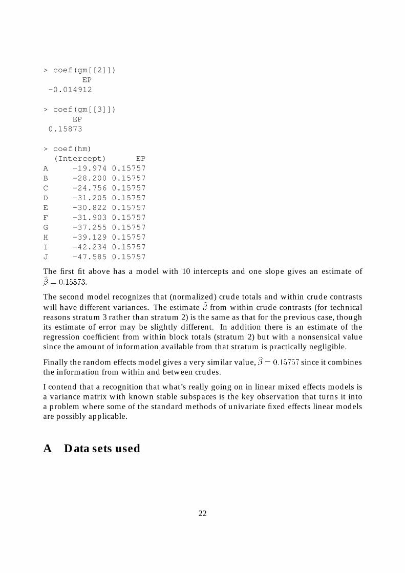
> coef(hm)(Intercept) EP

A -19.974 0.15757B -28.200 0.15757C -24.756 0.15757D -31.205 0.15757E -30.822 0.15757F -31.903 0.15757G -37.255 0.15757H -39.129 0.15757I -42.234 0.15757J -47.585 0.15757

The first fit above has a model with 10 intercepts and one slope gives an estimate ofb� = 0:15873.

The second model recognizes that (normalized) crude totals and within crude contrastswill have different variances. The estimate b� from within crude contrasts (for technicalreasons stratum 3 rather than stratum 2) is the same as that for the previous case, thoughits estimate of error may be slightly different. In addition there is an estimate of theregression coefficient from within block totals (stratum 2) but with a nonsensical valuesince the amount of information available from that stratum is practically negligible.

Finally the random effects model gives a very similar value, b� = 0:15757 since it combinesthe information from within and between crudes.

I contend that a recognition that what’s really going on in linear mixed effects models isa variance matrix with known stable subspaces is the key observation that turns it intoa problem where some of the standard methods of univariate fixed effects linear modelsare possibly applicable.

A Data sets used

22

Density 24.7 24.8 27.3 28.4 28.4 29.0 30.3 32.7 35.6 38.5 38.8 39.3

Hardness 484 427 413 517 549 648 587 704 979 914 1070 1020

Density 39.4 39.9 40.3 40.6 40.7 40.7 42.9 45.8 46.9 48.2 51.5 51.5

Hardness 1210 989 1160 1010 1100 1130 1270 1180 1400 1760 1710 2010

Density 53.4 56.0 56.5 57.3 57.6 59.2 59.8 66.0 67.4 68.8 69.1 69.1

Hardness 1880 1980 1820 2020 1980 2310 1940 3260 2700 2890 2740 3140

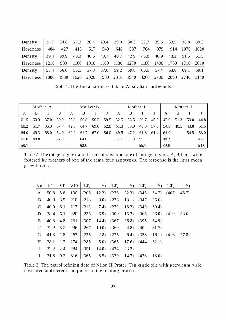
Table 1: The Janka hardness data of Australian hardwoods.

Mother: A Mother: B Mother: I Mother: J

A B I J A B I J A B I J A B I J

61.5 60.3 37.0 59.0 55.0 50.8 56.3 59.5 52.5 56.5 39.7 45.2 42.0 51.3 50.0 44.8

68.2 51.7 36.3 57.4 42.0 64.7 69.8 52.8 61.8 59.0 46.0 57.0 54.0 40.5 43.8 51.5

64.0 49.3 68.0 54.0 60.2 61.7 67.0 56.0 49.5 47.2 61.3 61.4 61.0 54.5 53.0

65.0 48.0 47.0 64.0 52.7 53.0 55.3 48.2 42.0

59.7 62.0 55.7 39.6 54.0

Table 2: The rat genotype data. Litters of rats from one of four genotypes, A, B, I or J, werefostered by mothers of one of the same four genotypes. The response is the litter meangrowth rate.

No SG VP V10 (EP, Y) (EP, Y) (EP, Y) (EP, Y)

A 50.8 8.6 190 (205, 12.2) (275, 22.3) (345, 34.7) (407, 45.7)

B 40.8 3.5 210 (218, 8.0) (273, 13.1) (347, 26.6)

C 40.0 6.1 217 (212, 7.4) (272, 18.2) (340, 30.4)

D 38.4 6.1 220 (235, 6.9) (300, 15.2) (365, 26.0) (410, 33.6)

E 40.3 4.8 231 (307, 14.4) (367, 26.8) (395, 34.9)

F 32.2 5.2 236 (267, 10.0) (360, 24.8) (402, 31.7)

G 41.3 1.8 267 (235, 2.8) (275, 6.4) (358, 16.1) (416, 27.8)

H 38.1 1.2 274 (285, 5.0) (365, 17.6) (444, 32.1)

I 32.2 2.4 284 (351, 14.0) (424, 23.2)

J 31.8 0.2 316 (365, 8.5) (379, 14.7) (428, 18.0)

Table 3: The petrol refining data of Nilon H Prater. Ten crude oils with petroleum yieldmeasured at different end points of the refining process.

23

Year Rain0 Temp1 Rain1 Temp2 Rain2 Temp3 Rain3 Temp4 Yield

1930 17.75 60.2 5.83 69.0 1.49 77.9 2.42 74.4 34.01931 14.76 57.5 3.83 75.0 2.72 77.2 3.30 72.6 32.91932 27.99 62.3 5.17 72.0 3.12 75.8 7.10 72.2 43.01933 16.76 60.5 1.64 77.8 3.45 76.4 3.01 70.5 40.01934 11.36 69.5 3.49 77.2 3.85 79.7 2.84 73.4 23.01935 22.71 55.0 7.00 65.9 3.35 79.4 2.42 73.6 38.41936 17.91 66.2 2.85 70.1 0.51 83.4 3.48 79.2 20.01937 23.31 61.8 3.80 69.0 2.63 75.9 3.99 77.8 44.61938 18.53 59.5 4.67 69.2 4.24 76.5 3.82 75.7 46.31939 18.56 66.4 5.32 71.4 3.15 76.2 4.72 70.7 52.21940 12.45 58.4 3.56 71.3 4.57 76.7 6.44 70.7 52.31941 16.05 66.0 6.20 70.0 2.24 75.1 1.94 75.1 51.01942 27.10 59.3 5.93 69.7 4.89 74.3 3.17 72.2 59.91943 19.05 57.5 6.16 71.6 4.56 75.4 5.07 74.0 54.71944 20.79 64.6 5.88 71.7 3.73 72.6 5.88 71.8 52.01945 21.88 55.1 4.70 64.1 2.96 72.1 3.43 72.5 43.51946 20.02 56.5 6.41 69.8 2.45 73.8 3.56 68.9 56.71947 23.17 55.6 10.39 66.3 1.72 72.8 1.49 80.6 30.51948 19.15 59.2 3.42 68.6 4.14 75.0 2.54 73.9 60.51949 18.28 63.5 5.51 72.4 3.47 76.2 2.34 73.0 46.11950 18.45 59.8 5.70 68.4 4.65 69.7 2.39 67.7 48.21951 22.00 62.2 6.11 65.2 4.45 72.1 6.21 70.5 43.11952 19.05 59.6 5.40 74.2 3.84 74.7 4.78 70.0 62.21953 15.67 60.0 5.31 73.2 3.28 74.6 2.33 73.2 52.91954 15.92 55.6 6.36 72.9 1.79 77.4 7.10 72.1 53.91955 16.75 63.6 3.07 67.2 3.29 79.8 1.79 77.2 48.41956 12.34 62.4 2.56 74.7 4.51 72.7 4.42 73.0 52.81957 15.82 59.0 4.84 68.9 3.54 77.9 3.76 72.9 62.11958 15.24 62.5 3.80 66.4 7.55 70.5 2.55 73.0 66.01959 21.72 62.8 4.11 71.5 2.29 72.3 4.92 76.3 64.21960 25.08 59.7 4.43 67.4 2.76 72.6 5.36 73.2 63.21961 17.79 57.4 3.36 69.4 5.51 72.6 3.04 72.4 75.41962 26.61 66.6 3.12 69.1 6.27 71.6 4.31 72.5 76.0

Table 4: The Iowa wheat yield data. The yield (in bushels/acre) for the state of Iowa,with average monthly temperatures and rainfalls as covariates. The year is a surrogatefor variety improvements.

24

References

Draper, N. R. and Smith, H. (1981). Applied Regression Analysis, second edn, Wiley, NewYork.

Hastie, T. J. and Tibshirani, R. J. (1990). Generalized Additive Models, Chapman & Hall,London/New York.

SAS Institute Inc. (1990). SAS/STAT User’s Guide, Version 6, Vol. 1, fourth edition edn, SASInstutute, Inc., Cary, NC.

Prater, N. H. (1956). Estimate gasoline yields from crudes, Petroleum Refiner 35: 236–238.

Scheffe, H. (1959). The Analysis of Variance, Wiley, New York.

Williams, E. J. (1959). Regression Analysis, Wiley, New York.

25