New J. Phys. 18 (2016) 045010 doi:10.1088/1367-2630/18/4/045010

PAPER

A coordinate Bethe ansatz approach to the calculation of equilibriumand nonequilibrium correlations of the one-dimensional Bose gas

JanCZill1, TodMWright1, KarénVKheruntsyan1, ThomasGasenzer2,3 andMatthew JDavis1,4

1 School ofMathematics andPhysics, TheUniversity of Queensland, BrisbaneQLD4072, Australia2 Kirchhoff-Institut für Physik, UniversitätHeidelberg, ImNeuenheimer Feld 227,D-69120Heidelberg, Germany3 ExtreMeMatter Institute EMMI,GSIHelmholtzzentrum für Schwerionenforschung, D-64291Darmstadt, Germany4 JILA,University of Colorado, 440UCB, Boulder, CO80309,USA

E-mail: j.zill@uq.edu.au

Keywords:Bethe ansatz, one-dimensional quantumgases, few-body systems, Lieb–Linigermodel

AbstractWeuse the coordinate Bethe ansatz to exactly calculatematrix elements between eigenstates of theLieb–Linigermodel of one-dimensional bosons interacting via a two-body delta-potential.Weinvestigate the static correlation functions of the zero-temperature ground state and their dependenceon interaction strength, and analyze the effects of system size in the crossover from few-body tomesoscopic regimes for up to seven particles.We also obtain time-dependent nonequilibriumcorrelation functions forfive particles following quenches of the interaction strength from twodistinctinitial states. One quench is from the noninteracting ground state and the other from a correlatedground state near the strongly interacting Tonks–Girardeau regime. Thefinal interaction strength andconserved energy are chosen to be the same for both quenches. The integrability of themodel highlyconstrains its dynamics, andwe demonstrate that the time-averaged correlation functions followingquenches from these two distinct initial conditions are both nonthermal andmoreover distinct fromone another.

1. Introduction

The Lieb–Linigermodel of a one-dimensional (1D)Bose gaswith repulsive delta-function interactions is aparadigmatic example of an exactly solvable continuous, integrablemany-body quantum system [1]. Inparticular, it has served as the context for the development of theoretical tools that have subsequently beenwidely applied in the study of integrable systems, such as the so-called ‘thermodynamic Bethe ansatz’ functionalrepresentation, which provides the exact equation of state, excitation spectrum [1], and bulk parameters [2] ofthe system in the thermodynamic limit. However, the calculation of correlation functions from the exactsolutions provided by the Bethe ansatz is notoriously difficult.

At zero temperature, exact closed-form solutions for some equilibrium correlation functions are known inthe Tonks–Girardeau limit of infinite interaction strength [3–7]. This comparatively tractable limit also allowsfor some strong-coupling expansion results for large butfinite interactions [7–10]. In the opposite weaklyinteracting quasi-condensate regime, amean-field approach can be used to describe the system [11] and aBogoliubovmethod can be used to determine the low-lying excitation spectrum [12], relying on small densityfluctuations. Fewer results are available for intermediate interaction strengths, away from the stronglyinteracting andweakly interacting regimes. The development of the Luttinger liquid description of quantumfluids [13] and the related formalismof conformal field theory [14, 15] have lead to the prediction of power-lawscaling forfirst-order correlations at large distances, with an exponent given in terms of the equation of state thatis known exactly from the thermodynamic Bethe ansatz [16]. The algebraic Bethe ansatz provides adeterminantal representation of correlations, fromwhich their asymptotic behavior can be extracted [17].Morerecently, exact expressions for local second- and third-order correlations [18–20], together with exact results for

OPEN ACCESS

RECEIVED

4 January 2016

REVISED

24 February 2016

ACCEPTED FOR PUBLICATION

15March 2016

PUBLISHED

13April 2016

Original content from thisworkmay be used underthe terms of the CreativeCommonsAttribution 3.0licence.

Any further distribution ofthis workmustmaintainattribution to theauthor(s) and the title ofthework, journal citationandDOI.

© 2016 IOPPublishing Ltd andDeutsche PhysikalischeGesellschaft

the one-body correlation function at asymptotically short distances [21] in terms of the equation of state havebeen derived.

Away from the asymptotic short- and long-range regimes, the behavior of correlation functions is less wellknown. For intermediate interaction strengths and arbitrary length scales onemust resort to numerics todetermine the correlation functions. Results for the latter have been obtained using numericalmethodologiesincluding quantumMonteCarlo [22, 23], and densitymatrix renormalization group approaches [24]. A recentlydeveloped, integrability-based approach combines the decomposition of correlation functions into sums overmatrix elements (form factors) of certain simple operators betweenBethe ansatz eigenstates [25, 26]. Thisapproach has generated results, for example, for static and dynamical equilibrium correlations at zero and finitetemperaturefor systems of up to »N 100 particles [27]. Other finite temperature results for correlationfunctions have been obtained using imaginary time stochastic gaugemethods [28, 29], taking the nonrelativisticlimit of a relativistic field theory [30], utilizing Fermi–Bosemapping for the strongly interacting gas [9, 31, 32],employing perturbative expansions in temperature and interaction strength [33], as well as combining thethermodynamic Bethe ansatz with theHellmann–Feynman theorem [34].

Experiments with ultracold quantumgases are able to realize effectively 1D systems by tightly confining thegas in two of the three spatial dimensions, either using optical lattice potentials or atom-chip traps [35–50].These experiments are nowprobing the predictions of the Lieb–Linigermodel. The configurability of quantum-gas experiments allows for so-called quenches of the system, inwhichHamiltonian parameters of the system areabruptly changed, and thus for the study of the Lieb–Lingermodel out of equilibrium, providing even greaterchallenges for theory.

The dynamically evolving correlations of the Lieb–Liniger gas in nonequilibrium scenarios are currently atopic of significant interest, and a number of theoretical approaches have been applied. Notable examplesinclude exact diagonalization under a lowmomentum cutoff [51–55], mapping of the hard-core Tonks–Girardeau gas to free spinless fermions [56–63], phase-spacemethods [64], dynamic Bogoliubov-likeapproximations [65] and tensor-networkmethods [66, 67]. References [68–71] employed nonperturbativeapproximative functional-integralmethods, while in [72] a dynamical Luttinger-liquid approachwas taken.Other calculationsmake explicit use of the integrability of the system. These are based on various Bethe ansatzapproaches, and include utilizing Fermi–Bosemapping [73, 74] and strong coupling expansions of thecoordinate Bethe ansatz wave function [75–77], combining the algebraic Bethe ansatz with other numericalmethods [78–80], and using the Yudson contour-integral representation for infinite-length systems [81, 82].Recently, it was conjectured that the dynamics following an interaction strength quench are captured by athermodynamic Bethe ansatz saddle point state and excitations around it—the so-called quench actionapproach [83–88]. In the spirit of themethodology of [25, 89], Gritsev et al [78] investigated a quench fromg = ¥0 by combining algebraic Bethe ansatz expressions for form factors with truncated sums over states,and employingMonte Carlo summation over the eigenstate components of the initial state.

In this paperwe take a different approach, and calculate correlation functions of the Lieb–Lingermodel,both in and out of equilibrium, by calculatingmatrix elements between Lieb–Liniger eigenstates directly withinthe coordinate Bethe ansatz formalism.Given the known expressions for the coordinate-space forms of Lieb–Liniger eigenstates, we generate symbolic expressions formatrix elements of operators between these states interms of the Bethe rapidities. The numerically obtained values of the rapidities can then be substituted to yieldessentially numerically exact values for thematrix elements.

In our previous workwe applied thismethodology to quenches from the ideal gas ground state to positive γfor up toN=5 particles [90]. In section 2we provide the details of themethodology, and describe how it can beused to calculate thematrix elements of the Lieb–Liniger eigenstates. These symbolic expressions, and thus thecomputational cost of evaluating them, grow combinatorially with particle number, restricting themethod tosystems of only a few particles. However for small particle numbers N 7 we obtain numerically exact resultsfor ground-state correlations, which are described in section 3. Our results demonstrate that local correlations inthe strongly interacting regime are already close to their thermodynamic-limit values for these few-body tomesoscopic systems.

An additional advantage of ourmethodology is that it can also calculate overlaps between Lieb–Linigereigenstates corresponding to any two interaction strengths, which allows us to study the dynamics of quenchesof the interaction strength between arbitrary values. In section 4we utilize this property to study the effects ofintegrability on the relaxation of the Lieb–Linigermodel following such a quench. In particular, we compare twononequilibriumquench scenarios with the samefinalHamiltonian and state energy, but beginning from starklydifferent initial states. Statisticalmechanics would predict that the systemwould relax to the same thermal statein both cases, but due to the integrability of the Lieb–Lingermodel not only are the time-averaged statesfollowing the two quenches nonthermal, they are also distinct. After characterizing and comparing thenonequilibriumdynamics following both quenches, we conclude in section 5.

2

New J. Phys. 18 (2016) 045010 J CZill et al

2. Coordinate Bethe-ansatzmethodology

2.1. Lieb–Linigermodel eigenstatesThe Lieb–Linigermodel [1] describes a systemofN indistinguishable bosons subject to a delta-functioninteraction potential in a periodic 1D geometry of length L.Wework in units such that = 1and the particlemass =m 1 2, and so theHamiltonian of this system reads

ˆ ( ) ( )å åd= -¶¶

+ -= <

Hx

c x x2 , 1i

N

i i j

N

i j1

2

2

where c is the interaction strength. The coordinate Bethe ansatz yields eigenstates ∣{ }l ñj ofHamiltonian(1)with spatial representation [17]

({ }) { }∣{ }

( ) ( )

{ }

{ } ( )( ) ( )

å å

z l

ll l

º á ñ

= --

-

l

ls

ss s= >

⎡⎣⎢

⎤⎦⎥

⎛⎝⎜

⎞⎠⎟

x x

A xc x x

exp i 1i sgn

, 2

i i j

m

N

m mk l

k l

k l1

j

j

where the rapidities lj (or quasimomenta) are solutions of the Bethe equations

( )ålp l l

= --

=

⎛⎝⎜

⎞⎠⎟L

mL c

2 2arctan . 3j j

k

Nj k

1

The quantumnumbersmj are anyN distinct integers (half-integers) in the case thatN is odd (even) [2], and åsdenotes a sumover all !N permutations { ( )}s s= j of { }N1, 2 ,..., . The normalization constant reads [17]

( )

[ ! { } [( ) ]]( ){ }

{ }

l l

l l=

-

- +l

l

>

>

AN M cdet

, 4k l k l

k l k l2 2 1 2j

j

where { }lMjis theN×Nmatrix with elements

[ ]( ) ( )

( ){ } ådl l l l

= ++ -

-+ -

l=

⎛⎝⎜

⎞⎠⎟M L

c

c

c

c

2 2. 5kl kl

m

N

k m k l12 2 2 2j

The rapidities determine the totalmomentum l= å =P jN

j1 and energy l= å =E jN

j12 of the system in each

eigenstate. The ground state of the system corresponds to the set ofN rapidities thatminimize E and constitutethe (pseudo-)Fermi sea of the 1DBose gas [17]. The Fermimomentum

( )p=

-k

L

N2 1

26F

is themagnitude of the largest rapidity occurring in the ground state in the Tonks–Girardeau limit of stronginteractions [3]. The only parameter of the Lieb–Linigermodel in the thermodynamic limit is the dimensionlesscoupling g º c n, where ºn N L is the 1Ddensity. Infinite systems, physical quantities also depend on theparticle numberN (see, e.g., section 3.3), whereas the length L of our system, and therefore also the density n, arearbitrary. Consequently, in this article wewill specify bothN and γ. Unless specified otherwise, wemeasure timein units of -kF

2, energy in units of kF2, and length in units of -kF

1.

2.2. Calculation of correlation functions and overlapsAs the eigenstates ∣{ }l ñj form a complete basis [91] for the state space of the Lieb–Linigermodel, the expectation

value ˆ { ˆ ( ) ˆ}rá ñ =O t OTrt of an arbitrary operator O in a Schrödinger-picture densitymatrix ˆ ( )r t can be

expressed as a sumofmatrix elements of O between the states ∣{ }l ñj . In particular, in a pure state∣ ( ) ( )∣{ }{ } { }y lñ = å ñl lt C t jj j

wehave

ˆ ( )∣ ˆ∣ ( ) ( ) ( ) { }∣ ˆ∣{ } ( ){ }{ }

{ } { }*ååy y l lá ñ º á ñ= á ¢ ñl l

l l¢

¢O t O t C t C t O , 7t j j

j j

j j

whereas in a statistical ensemblewith densitymatrix ˆ ∣{ } { }∣{ } { }r r l l= å ñál l j jSESE

j j, we find

ˆ { }∣ ˆ∣{ } ( ){ }

{ }år l lá ñ = á ñl

lO O . 8j jSE

j

j

3

New J. Phys. 18 (2016) 045010 J CZill et al

In this article, we focus in particular on the normalizedmth-order equal-time correlation functions

( )ˆ ( ) ˆ ( ) ˆ ( ) ˆ ( )

[ ˆ ( ) ˆ ( ) ˆ ( ) ˆ ( ) ]( )( )

† †

¢ ¢ ºáY Y Y ¢ Y ¢ ñ

á ñ á ñá ¢ ñ á ¢ ñg x x x x t

x x x x

n x n x n x n x,..., , ,..., ; , 9m

m mm m

m m1 1

1 1

1 11 2

where ˆ ( )(†)Y x is the annihilation (creation) operator for the Bose field and ˆ ( ) ˆ ( ) ˆ ( )†º Y Yn x x x . Here and in thefollowingwe drop the time index t of the state vectors.

Since theHamiltonianwe consider in this article is translationally invariant along the periodic volume oflength L, themean density ˆ ( )á ñ ºn x n is constant in both time and space, and

( ) ˆ ( ) ˆ ( ) ˆ ( ) ˆ ( )( ) † † ¢ ¢ = áY Y Y ¢ Y ¢ ñg x x x x t x x x x n,..., , ,..., ;mm m m m

m1 1 1 1 . The correlation functions

( )( ) ¢ ¢g x x x x t,..., , ,..., ;mm m1 1 can therefore be expressed as the expectation values of the operators

ˆ ( ) ˆ ( ) ˆ ( ) ˆ ( ) ˆ ( )( ) † † ¢ ¢ º Y Y Y ¢ Y ¢g x x x x x x x x n,..., , ,...,mm m m m

m1 1 1 1 .We note that for the same reasons as above

thematrix elements { }∣ ˆ ( )∣{ }( )l lá ¢ ¢ ¢ ñg x x x x,..., , ,...,jm

m m j1 1 are invariant under global coordinate shifts +x x d and thus, without loss of generality, we can set one of the spatial variables to zero. For the first-order

correlation function, thematrix elements are

{ }∣ ˆ ( )∣{ } { }∣ ˆ ( ) ˆ ( )∣{ }

( ) ( ) ( )

( ) †

{ } { } *ò

l l l l

z z

á ¢ ñ º á ¢ Y Y ñ

= l l- ¢ - -

g x x

N

nx x x x x x x

0, 0

d d 0, ,..., , ,..., . 10

j j j j

N N N

1

1 1 1 1 1 1j j

The evaluation of the integral in equation (10) is complicated by the sign function in equation (2) and theassociated nonanalyticities in ({ }){ }z l xij

where any two particle coordinates xk and xl coincide. However, we can

use the Bose symmetry of thewave function ({ }){ }z l xijto reexpress thismatrix element as a sumof integrals

{ }∣ ˆ ( )∣{ } !

( ) ( ) ( )ℓ

ℓ ℓ

( )( )

{ } { }

ℓ

*

òål l

z z

á ¢ ñ =

´ l l

=

-

-

¢ - + -

-

g xN

nx x

x x x x x x x

0, d d

0, ,..., ,..., , , ,..., , 11

j j

N

xN

N N

1

0

1

1 1

1 1 1 1 1

N

j j

1,

over the ordered domains [10]

( ) ( ) < < < < < <+x x x x x x L: 0 . 12M j j j M, 1 1

Substituting the coordinate-space form (equation (2)) of the Lieb–Liniger eigenfunctions, we obtain

{ }∣ ˆ ( )∣{ } !

( ) ( )

( )ℓ

ℓ

( ){ } { }

( ) ( ) ( ) ( )

( )( )

( ) ( )ℓ

ℓ( )

*

ò

åå

å å

l ll l l l

l l l

á ¢ ñ = --

+¢ - ¢

´ - ¢

l ls s s s s s

s s s

¢¢ > ¢> ¢ ¢ ¢ ¢ ¢

=

-

+ -=

-

¢ +-

+

⎛⎝⎜

⎞⎠⎟

⎛⎝⎜⎜

⎞⎠⎟⎟

⎛⎝⎜

⎞⎠⎟

g xN

nA A

c c

x x x x

0, 1i

1i

exp i d d exp i ,

13

j jj k j k j k j k

N

xN

m

N

m m m

1

0

1

1 1 11

1

1

j j

N 1,

1

where ℓ ℓ( ( ) ( ) ( ) ( ))ℓ( )s s s s s= ++ N1 ,..., , 2 ,...,1 . Thematrix elements of the second-order correlation

operator ˆ ( ) ˆ ( ) ˆ ( ) ˆ ( ) ˆ ( )( ) † †º Y Y Y Yg x x x n0, 0 02 2 are similarly given by

{ }∣ ˆ ( )∣{ } !

( ( ) )

( ) ( )

ℓℓ ℓ

( ){ } { }

( ) ( ) ( ) ( )

( ) ( )( )

( ) ( )

ℓ

ℓ ℓ( ) ( )

*

ò

åå

å

å

l ll l l l

l l

l l

á ¢ ñ = --

+¢ - ¢

´ - ¢

´ - ¢

l ls s s s s s

s s

ss

¢¢ > ¢> ¢ ¢ ¢ ¢ ¢

=

-

+ ¢ + -

=

-

¢

-

+ +

⎛⎝⎜

⎞⎠⎟

⎛⎝⎜⎜

⎞⎠⎟⎟

⎛⎝⎜

⎞⎠⎟

g xN

nA A

c c

x x x

x

0, 1i

1i

exp i d d

exp i , 14

j jj k j k j k j k

N

xN

m

N

mm

m

22

0

2

2 2 1 2

1

2

j j

N 2,

1, 2 1, 2

where ℓ ℓ( ( ) ( ) ( ) ( ))ℓ( )s s s s s= + ++ N2 ,..., 1 , 3 ,...,1, 2 andℓ( )s¢ +1, 2

is defined analogously in terms of theelements of s¢. In the limit x 0 this expression simplifies somewhat, and in general thematrix elements of the

localmth-order correlation operator ˆ ( ) [ ˆ ( )] [ ˆ ( )]( ) †º Y Yg n0 0 0m m m m are given by the expression

{ }∣ ˆ ( )∣{ } !

( ) ( )ℓ

( ){ } { }

( ) ( ) ( ) ( )

( ) ( )

*

ò

åå

å å

l ll l l l

l l

á ¢ ñ = --

+¢ - ¢

´ - ¢

l ls s s s s s

s s

¢¢ > ¢> ¢ ¢ ¢ ¢ ¢

=

-

-=

-

+ ¢ +-

⎛⎝⎜

⎞⎠⎟

⎛⎝⎜⎜

⎞⎠⎟⎟

⎛⎝⎜

⎞⎠⎟

gN

nA A

c c

x x x

0 1i

1i

d d exp i , 15

jm

j mj k j k j k j k

N m

N mn

N m

m n m n n0

11

j j

N m

4

New J. Phys. 18 (2016) 045010 J CZill et al

where the domain < < <x x x L: 0M M1 2 .We note,moreover, that equations (13)–(15) include asdegenerate cases the diagonalmatrix elements (see [10]) appropriate to the calculation of correlations in theground state (section 3) and in statistical ensembles (section 4).

The calculation of correlation functions from equations (13)–(15) involves the evaluation of integrals of thegeneral form

( )

ℓ

ℓ ℓ

( )ℓ

ℓℓ ℓ

ℓ ℓℓ

ℓ ℓ

ò ò ò ò

ò ò ò

åk =

´

k k k

k k k

=- +

-

- -+

+ +

- -

⎛⎝⎜

⎞⎠⎟x x x x x x

x x x

d d exp i d e d e d e

d e d e d e ,

16

xM

m

M

m mx

L

Mx

x

x

Mx

x

xx

xx

xx

xx

11

i1

i1

i

0

i

01

i

01

i

M

M MM

M M

,

1 12

1 1

1 12

1 1

where (for the repulsive interactions >c 0 considered in this article) the km are real numbers. A single closedform for this integral does not exist, as in general one ormore km may vanish, and thismust be handledseparately from the case of k ¹ 0m . However, given knowledge of the particular sets of rapidities { }lj and { }l¢j(and permutationsσ and s¢), and thus of the locations of zero exponents k = 0m in equation (16), eachindividual integral of this form can be reduced to an algebraic expression in terms of { }km .More specifically,each successive integration ò xd m yields a term (involving, in general, +xm 1) arising from the primitive integral[92]

( ) ( )

!( ) ( )!

( )

òå

=- G + -

=--

+

+

=

x x k p kx

p kkx

s

d e i 1, i

i ei

, 17

p kx p

p kx

s

p s

i 1

1 i

0

in the case that km is nonzero, or from ò x xd p otherwise. In our calculations, the construction of algebraicexpressions for the integrals occurring in equations (13)–(15) in terms of the rapidities lj is efficiently performedby a simple computer algorithm that accounts for and combines the symbolic terms that arise from thesesuccessive reductions.We note that, e.g., eachmatrix element { }∣ ˆ ( )∣{ }( )l lá ¢ ñg x0,j j

1 is a sumofN integrals over( )-N 1 -dimensional domains and that the integrand in each case comprises ( !)N 2 terms [10], illustrating thedramatically increasing computational cost of evaluating correlation functionswith increasingN. Nevertheless,the explicit closed-form expression for the integral produced by our algorithm can be evaluated to obtain anumerically exact result by substituting in the values of the rapidities. The latter are obtained by solvingequation (3)numerically usingNewton’smethod, starting in the Tonks–Girardeau regime of strong interactionsg 1and iteratively progressing to smaller values of γ using initial guesses given by linear extrapolation of the

solutions at stronger interaction strengths.We note that this algorithmic approach also provides for the efficient and accurate calculation of the

overlaps { }∣{ }l má ñj j between eigenstates ofHamiltonian(1) corresponding to different values of γ, whichwemake use of in our analysis of nonequilibriumdynamics in section 4. In particular, the overlap between anarbitrary eigenstate ∣{ }l ñj of H at afinite interaction strength g > 0 and the noninteracting ground state ∣ ñ0 ,

with constant spatial representation { }∣á ñ = -x L0iN 2, is simply given by

{ }∣ ! ( ){ }( ) ( )

( )òå ål

l llá ñ = +

--l

s s ss

> =

⎛⎝⎜

⎞⎠⎟

⎛⎝⎜

⎞⎠⎟

N

LA

cx x x0 1

id d exp i , 18j N

j k j kN

n

N

n n2 11

jN

which can easily be evaluated semi-analytically using our algorithm. In practice wefind that the results we obtainfor the overlaps fromour evaluation of equation (18) agreewith the recently derived closed-form expressions forthese quantities [84, 93–95], which imply in particular that { }∣l lá ñ µ0 1j j

2 as any l ¥j .

3.Ground-state correlation functions

As afirst application of ourmethodologywe calculate the correlation functions of the Lieb–Linigermodel in theground state for up toN=7 particles. In this case, we need to evaluate only the diagonal elements ofequations (13)–(15) in the ground-state wave function, thereby obtaining exact algebraic expressions forcorrelation functions in terms of the ground-state rapidities, which are themselves determined tomachineprecision (section 2.2). The ground-state correlations of the Lieb–Linigermodel have been consideredextensively in previousworks (see [96, 97] and references therein), andwe compare our exactmesoscopic resultsto those obtainedwith various othermethods and approximations, forfinite system sizes as well as in thethermodynamic limit. This allows us to clarify the utility and limitations of calculations, such as ours here and in[90], that involve only small particle numbers.

5

New J. Phys. 18 (2016) 045010 J CZill et al

3.1. First-order correlationsWebegin by considering thefirst-order correlation function ( ) ( )( ) ( )ºg x g x0,1 1 in the ground state of the Lieb–Linigermodel. Infigure 1(a)weplot ( )( )g x1 forN=7 particles for a range of interaction strengths γ, whichexhibits the expected decrease in spatial phase coherencewith increasing γ [16]. As is well known, true long-range order, ( )( ) = >¥ g x nlim 0x

10 [98, 99], is prohibited in an interacting homogeneous 1DBose gas in the

thermodynamic limit, even at zero temperature (see [97] and references therein). Indeed the Lieb–Linigersystem is quantum critical at zero temperature, and the asymptotic long-range behavior of ( )( )g x1 is a power-lawdecay (so-called quasi-long-range order) [17].

This power-law scaling of ( )( )g x1 is only expected to be realized at separations x large compared to thehealing length x g= 1 and, in afinite periodic geometry such as we consider here, is curtailed by the finiteextent L of the system(see, e.g., [16]). Indeed, for g = 0.1, the power-law decay is not visible in our finite-sizedcalculation, although as the interaction strength γ increases ( )( )g x1 exhibits behavior consistent with power-lawdecay over an increasingly large range of x, seefigure 1(a). In particular, for g 10, our results for ( )( )g x1 seemto converge toward the asymptotic scaling of the Tonks–Girardeau limit (black dotted–dashed line)withincreasing γ.

Due to the translational invariance of our system, thefirst-order correlations of the Lieb–Liniger groundstate are encoded in themomentumdistribution

( ) ( ) ( )( ) ò= -n k n x g xd e , 19j

Lk x

0

i 1j

which, in ourfinite periodic geometry, is only defined for discretemomenta p=k j L2j , with j an integer. Infigure 1(b)weplot themomentumdistributions ( )n kj corresponding to the first-order correlation functions

( )( )g x1 shown infigure 1(a). Thefirst feature thatwe note infigure 1(b) is that for all interaction strengths, ( )n kexhibits a power-law decay ( ) µ -n k k 4 (dotted–dashed black line) at highmomenta. This is a universal resultfor delta-function interactions in 1D [21, 89, 100] (and indeed also in higher dimensions [101]). The effects ofthefinite extent L of the systemon the first-order correlations are again evident in thismomentum-spacerepresentation. For g = 0.1, no deviation from the∝k−4 scaling is observed for the smallest (nonzero)momentakj that can be resolved in the periodic geometry. For larger values of the interaction strength, ( )n k departs fromthe∝k−4 scaling at increasingly large values of kwith increasing γ, and develops a hump atmomenta near kF forg 10 [89].We note that although the small-k behavior of ( )n k tends towards theµ -k 1 2 scaling exhibited by

the Tonks–Girardeau gas in the thermodynamic limit, the rounding off of the power-law decay of ( )( )g x1 asx L 2 precludes ( )n k from reaching the known asymptotic k 0 behavior in our finite geometry.

Figure 1.One- and two-body correlations in the Lieb–Liniger ground state, forN=7 particles. (a)Nonlocal first-order coherence( )( )g x1 . The black dotted–dashed line indicates the asymptotic long-range behavior ( ) ∣ ∣( ) µ -g x x1 1 2 of a Tonks–Girardeau gas in the

thermodynamic limit. (b)Corresponding zero-temperaturemomentumdistribution ( )n kj . The black dotted–dashed line indicatesthe universal high-momentumpower-law scaling ( ) µ -n k k 4 common to all positive interaction strengths [21]. (c)Nonlocal second-order coherence ( )( )g x2 . (d)Corresponding static structure factor S(k).

6

New J. Phys. 18 (2016) 045010 J CZill et al

3.2. Second-, third-, and fourth-order correlationsInfigure 1(c), we present the nonlocal second-order coherence ( ) ( )( ) ( )ºg x g x x0, , , 02 2 , which provides ameasure of density-density correlations, forN=7 particles at a range of interaction strengths γ. In the limitingcase of an ideal gas (g = 0), the ground state of the system is a Fock state ofN particles in the zero-momentumsingle-particlemode, and the second-order coherence ( )( ) = -g=

-g x N10

2 1 (horizontal dashed line) is thereforeindependent of x. As the interaction strength γ is increased, the second-order coherence is increasinglysuppressed at zero spatial separation and correspondingly enhanced at separations -x k2 F

1. Oscillations in( )( )g x2 develop atfinite x as the system enters the strongly interacting regime g 1 [9, 17] and, in particular, for

g = 100 (dashed cyan line), our numerical results are practically indistinguishable from the exact Tonks–Girardeau limit result (solid black line) [3].

An alternative representation of the second-order correlations of the ground state is given by the staticstructure factor S(k), which is related to ( )( )g x2 by [11]

( ) [ ( ) ] ( )( )ò= + --S k n x g x1 d e 1 . 20j

Lk x

0

i 2j

Infigure 1(d)we present the structure factors S(k) corresponding to the correlation functions ( )( )g x2 shown infigure 1(c). For all values of γ, ( ) =S 0 0 due to particle-number conservation and translational invariance. In theideal-gas limit (red circles) ( ) =S k 1j for all nonzero kj. In the opposite limit of a Tonks–Girardeau gas

( )∣ ∣( )

∣ ∣

∣ ∣( )

=

-

>g=¥

-⎧⎨⎪⎩⎪

S k

k N

kk k

k k

1

22

1 2 ,

21j

jj

j

1

FF

F

which tends, in the thermodynamic limit, to thewell-known result (see, e.g., [9]) ( ) ∣ ∣=S k k k2 F for ∣ ∣ k k2 F,and ( ) =S k 1 for ∣ ∣ >k k2 F. Just as for ( )( )g x2 , we observe that for g = 100 (cyan plus symbols), our numericalresults for S(k) are almost identical to the known exact expression (equation (21)) for the Tonks–Girardeau limit(black crosses). For smaller values of γ ourmesoscopic results for S(k) appear consistent with those of [22, 25],obtained using quantumMonteCarlo and algebraic-Bethe ansatz techniques, respectively.

We now focus inmore detail on local correlation functions.We note that the local second-order coherencehas recently been proposed as ameasure of quantum criticality in the 1Dboson system [102], while the localthird-order correlations have received increasing attention both in theory [103] and experiment [47, 104–106].The local fourth-order correlations for the Lieb–Linigermodel have also been investigated [107]. Infigure 2, weplot the local second-order coherence ( )( )g 02 (solid red line), together with the local third-order coherence

( ) [ ˆ ( )] [ ˆ ( )]( ) †= á Y Y ñg n0 0 03 3 3 3 (dotted green line), and the local fourth-order coherence

( ) [ ˆ ( )] [ ˆ ( )]( ) †= á Y Y ñg n0 0 04 4 4 4 (dashed blue line) forN=7 particles and a broad range of interactionstrengths γ. For comparison, we also plot the asymptotic results obtained in the Bogoliubov limit of weakinteractions (g 0) in the thermodynamic limit [12, 18] (left-hand dotted–dashed lines). The numericalresults for small γ are broadly comparable to these thermodynamic-limit results. However, for the small particlenumbers considered here, the suppression of ( )( )g 02 , ( )( )g 03 , and ( )( )g 04 due to interactions in the limit of smallγ is overshadowed by the suppression due to the finite population of the system [20]. At larger γ, the effects ofinteractions dominate, and the numerical results converge closely to the appropriate strong-couplingexpressions [18] (right-hand dotted–dashed lines).We note, therefore, that the local correlations of the Lieb–

Figure 2. Interaction-strength dependence of the local second-, third- and fourth-order coherence in the Lieb–Liniger ground state,forN=7 particles. To aid visibility, we plot ( )( )g 02 scaled by a factor of 101, and ( )( )g 04 scaled by a factor of 10−1. Dotted–dashedlines indicate asymptotic weak- ( g 1) and strong-coupling ( g 1) expressions for ( )( )g 02 , ( )( )g 03 and ( )( )g 04 in thethermodynamic limit (see text).

7

New J. Phys. 18 (2016) 045010 J CZill et al

Liniger ground state, and particularly their scalingwith γ, appear to be quite insensitive to the infrared cutoffimposed by thefinite extent of our system in the strongly interacting regime g 1.

3.3. System-size dependenceThe results we have obtained so far indicate that, as expected, the small size of our system leads to corrections tocorrelation functions as compared to their known asymptotic forms in the thermodynamic limit. However, ourresults also suggest that the effects offinite system size are comparatively less important for local correlations,particularly in the limit of large interaction strengths g 1. To further elucidate the potential significance offinite-size effects in our calculations of nonequilibriumdynamics [90], here we give a brief characterization ofthe dependence of correlation functions of the Lieb–Liniger ground state on the particle numberN at afixedvalue of the interaction strength γ.

Specifically we consider the case for g = 10, as this value places the system in the strongly interacting regimeg 1 (which appears less sensitive tofinite-size effects than theweakly interacting regime g 1), while still

exhibiting significant deviations from the Tonks–Girardeau limit (see, e.g., [9]).Whereas elsewhere in this paperwe quotemomenta (lengths) in units of kF ( -kF

1), in comparing results between systemswith different particlenumbersNwe quotemomenta (lengths) in units of pn [( )p -n 1], so as to avoid a potentiallymisleadingdependence of the unit of length onN (see equation (6)).

Infigure 3(a)weplot ( )( )g x1 for particle numbers =N 3, 4, 5, 6, and 7. For small x, the curves fall nearlyperfectly on one line. The same behavior can be observed for the large-k tail of the correspondingmomentumdistribution ( )n k , whichwe plot infigure 3(b). Indeed, at largermomenta pk n2 , ( )n k appears to exhibit arapid collapse to a single curvewith increasingN [21, 109]. However, the differences in ( )n k are so small thatthey can not be seen infigure 3(b). For smallmomenta, our choice of units implies an increasing resolutionwithincreasing particle number, specifically ( )p p= ´ =-k L n N2 21

1 . However, this lowest resolvablemomentum seems to fall on one line for increasing particle number, indicating that the infrared behavior oflarge systems can be at least partly accessed by ourmesoscopic system sizes.

Luttinger-liquid theory predicts a long-range power-law decay ( ) ∣ ∣( ) µ -g x x K1 1 2 , where the LuttingerparameterK can be calculated from the thermodynamic limit of the Bethe ansatz solution (see, e.g., [16, 17] andreferences therein). For our parameters we haveK=1.40, implying an asymptotic scaling ( ) ∣ ∣( ) µ -g x x1 0.357

(black dotted–dashed line infigure 3(a)). This corresponds to a power-law behavior( ) ∣ ∣ ∣ ∣ µ =- + -n k k kK1 1 2 0.643 [16] (dotted–dashed line infigure 3(b)) for smallmomenta.We note that this

infrared scaling is a truemany-body effect and as such does not showup forN=2 particles. Indeed, one canshow analytically that, forN=2, themomentumdistribution ( ) ( ) lµ - -n k k1

2 2 2 and thus -k 4 is the highestpower in the series expansion of ( )n k .

Figure 3.Dependence offirst- and second-order correlations in the Lieb–Liniger ground state on particle numberN for g = 10. (a)First-order correlation function ( )( )g x1 . (b)Correspondingmomentumdistribution function ( )n kj . Black dotted–dashed lines in (a)and (b) indicate the asymptotic infrared scaling of ( )( )g x1 and ( )n k , respectively, with Luttinger parameterK=1.40 (see text). (c)Second-order correlation function ( )( )g x2 . (d)Corresponding static structure factor S(k). The black dotted–dashed lines in (c) and (d)represent the phenomenological expressions of [108] for ( )( )g x2 and S(k) in the thermodynamic limit, respectively.

8

New J. Phys. 18 (2016) 045010 J CZill et al

Infigure 3(c)weplot the nonlocal second-order coherence ( )( )g x2 for g = 10 and =N 3, 4, 5, 6, and 7.The corresponding static structure factor S(k) is shown infigure 3(d). Infigure 3(d)we also plot (black dotted–dashed line) the formof S(k) resulting from the phenomenological expression proposed in [108] (see also [110]).This expression involves the limiting dispersions and edge exponents of the Lieb–Linigermodel, whichweobtain by numerically solving the appropriate integral equations [1, 111].We also plot the correspondingprediction for ( )( )g x2 (black dotted–dashed line) infigure 3(c).We note that the numerical results for ourmesoscopic systems are, in general, rather close to the phenomenological thermodynamic-limit expressionseven for the relatively small particle numbers considered here.

4. Application to nonequilibriumdynamics

Wenow apply ourmethodology to the nonequilibriumdynamics of the Lieb–Linigermodel. Specifically, weconsider the evolution of a system, initially prepared in the ground state ofHamiltonian(1)with interactionstrength g0, following an abrupt change, at time t=0, of the interaction strength to a distinct value g g¹ 0—a so-called ‘interaction quench’. The evolution of the system following such a quench is generated byHamiltonian(1)with interaction strength γ, whichwe denote by ˆ ( )gH hereafter. The time-evolving state isgiven at all times >t 0 by

∣ ( ) ∣{ } ( ){ }

{ } { }åy lñ = ñl

l-t C e , 22E t

ji

j

jj

where ∣{ }l ñj are the eigenstates of ˆ ( )gH with energies { }lEj, and { }∣{ } l yº á ñlC j 0j

are the overlaps of the ∣{ }l ñj

with the initial state ∣y ñ0 . The expectation value of an arbitrary operator O in the state ∣ ( )y ñt is given by

ˆ ( )∣ ˆ∣ ( ) { }∣ ˆ∣{ } ( ){ }{ }

{ } { }( ){ } { }*ååy y l lá ñ º á ñ= á ¢ ñ

l ll l

¢¢

-l l¢O t O t C C Oe . 23tE E t

j ji

j j

j jj j

Weuse themethodology described in section 2 to evaluate both the overlaps { }lCjand thematrix elements

{ }∣ ˆ∣{ }l lá ¢ ñOj j that appear in equation (23).One of the features of ourmethodology is that it allows us to describe quenches between arbitrary interaction

strengths. In this paperwe consider two interaction-strength quenches, fromdifferent initial interactionstrengths g0, to a common final value of the coupling γ. Specifically, we consider a quench from thenoninteracting limit g = 00 (similar to those previously studied in [63, 78, 84, 90, 112–115]) and a quench fromthe correlated ground state obtained for a strong interaction strength g = 1000 . As ˆ ( )gH is time independentfollowing the quench, energy is conserved during the dynamics.We choose thefinal interaction strength afterthe two quenches such that the postquench energy is the same in both cases.

The statistical description of the dynamics of sufficiently ergodic systems is usually based on the assumptionthat the energy is the sole integral ofmotion, such that the equilibrium system is entirely determined by itsenergy. If this would be the case for our system, the two quencheswould lead to the same equilibrium state.However, the dynamics according to the integrable Lieb–LinigerHamiltonian are strongly constrained by theconserved quantities other than the total energy. By performing two different quenches to the samefinalHamiltonian and energy, we investigate the effects of integrability on the postquench evolution of the Lieb–Liniger system.

The conserved energy following the quench is the energy of the system at time = +t 0 ,

( )∣ ˆ ( )∣ ( )

( ) ( ) ( ) ( )

y g y

g g gg

g

º á ñ

= + -

g g

g

+ +E H

EE

0 0

d

d, 24G 0 0

G

0

0

where ( )gEG 0 is the energy of the ground state ∣y ñ0 of the initialHamiltonian ˆ ( )gH 0 andwe used thewell-known

result ( ) ( )( ) g g=g- -g n N E0 d d2 2 1

G [18], which implies that g gE0

is given by following the tangent to the curve

( )gEG at g0 out to γ. Here, ( ) ∣ ˆ ( )∣( ) ( )y yº á ñgg g0 020

20

0is the local second-order coherence in the initial state. In

the case of a quench from the noninteracting ground state (g = 00 ), equation (24) reduces to the simpleexpression ( ) g= -gE N n10

2 [66, 90], implying that the energy imparted to the systemduring the quenchdiverges as g ¥ [63]. By contrast, in a quench from the Tonks–Girardeau limit g ¥0 to afiniteinteraction strength γ thefinal energy is bounded from above, ( ) ¥g¥E EG , by the ground-state energy ofthe Tonks–Girardeau gas. Nevertheless, according to equation (24), afinal interaction strength *g< <0 100such that * *=g g E E100 0 does exist.

Here, we consider quenches ofN=5 particles, and determine this final interaction strength tomachineprecision, inferring a value *g = 3.7660 ... fromnumerical solutions for the energy and local second-ordercoherence of the ground state atfinite γ (section 3.2).We note that although the overlaps { }lC

jof the initial state

9

New J. Phys. 18 (2016) 045010 J CZill et al

∣y ñ0 with the eigenstates of ˆ ( )*gH can be calculated analytically in the case of the quench from g = 00 [93–95],for the quench from g = 1000 no closed-form expressions for these quantities are known, and thus theirnumerical valuesmust be determined using the semi-analyticalmethodology described in section 2.2.

An important summary of the postquench expectation value of an operator (equation (23)) is provided bythe time-averaged value

( )∣ ˆ∣ ( ) ( )òt y y= á ñt

t

¥O t t O tlim

1d . 25

0

Neglecting degeneracies in the spectrumof ˆ ( )*gH (see discussion in appendix B), such averages are given by theexpectation values ˆ { ˆ ˆ}rá ñ =O OTrDE DE of operators O in the densitymatrix

ˆ ∣ ∣ ∣{ } { }∣ ( ){ }

{ }år l l= ñál

lC 26j jDE2

j

j

of the diagonal ensemble [116, 117].Formally, the sums in equations (22), (23), and (26) range over an infinite number of eigenstates ∣{ }l ñj , and

thus the basis over which ∣ ( )y ñt is expandedmust be truncated in our numerical calculations. By only includingeigenstates with an absolute initial-state overlap ∣ ∣{ }lC

jlarger than some threshold, we consistently neglect small

contributions to correlation functions fromweakly occupied eigenstates andminimize the truncation error for agiven basis size.We quantify this truncation error by the violations of the normalization and energy sum rules, aswe discuss in appendix A.

4.1. Evolution of two-body correlationsInfigure 4we plot the time evolution of the local second-order coherence ( )( )g t0,2 forN=5 particlesfollowing quenches of the interaction strength from initial values g = 00 (red dotted line) and g = 1000 (bluedashed line) to the common final value *g . For the quench from the noninteracting initial state (g = 00 ), as timeevolves the local second-order coherence decays from its initial value ( )( ) = = - -g t N0, 0 12 1before settlingdown tofluctuate about the diagonal-ensemble expectation value ( )( )g 0

DE2 (horizontal dotted–dashed line). This

behavior is consistent with results obtained for similar quenches of the interaction strength from zero to apositive value in [90]. For the quench from g = 1000 , the value of ( )( )g 02 in the initial ‘fermionized’ state is

( )( ) » -g 0 102 3. In this case ( )( )g t0,2 rises as time progresses, and then exhibits somewhat irregular oscillationsabout ( )( )g 0

DE2 (horizontal solid line).We observe that the decay (growth) of ( )( )g t0,2 to its diagonal-ensemble

value and the onset of irregular oscillations about this value occur on comparable time scales in the twoquenches.

We note that the predictions of the diagonal ensemble for the local second-order coherence ( )( )g 0DE

2 are very

similar for the two quenches, despite the significant difference between the values of ( )( )g 02 in the two initialstates. However, they are clearly distinct— ( )( )g 0

DE2 for the quench from the noninteracting state is in fact larger

than that for the quench from the correlated state by an amount≈0.0125, demonstrating that the system retainssomememory of its initial state in the long time limit as is expected for an integrable system.We analyze thisdifference inmore detail in section 4.3.

We now turn our attention to the time evolution of the full nonlocal second-order correlation function( )( )g x t,2 . Infigure 5(a)we show the dependence of ( )( )g x t,2 on separation x for the quench from the

noninteracting initial state at four representative times. (Note that the upper limit p= -x k2 F1of the x axis in

Figure 4.Time evolution of local second-order correlations forN=5 particles following quenches of the interaction strength to afinal value *g = 3.7660 ... from initial values g = 00 (red dotted line) and g = 1000 (blue dashed line). The horizontal solid (dotted–dashed) line indicates the prediction of the diagonal ensemble for ( )( )g 02 for the quench from g = 1000 (g = 00 ).

10

New J. Phys. 18 (2016) 045010 J CZill et al

figure 5(a) corresponds to =x L 2 in the present case ofN= 5 particles.)At t=0 (horizontal solid line), thesecond-order coherence has the constant formof the noninteracting ground state. At short times (e.g.,= -t k0.01 F

2, red dashed line) aminimum in ( )( )g x2 develops at zero separation, togetherwith the

correspondingmaximum required by the conservation of ( )( )ò x g x td ,L

0

2 [66]. As time progresses awave

pattern ofmaxima andminima develops and propagates away from the origin (e.g., = -t k0.1 F2, green dotted

line). By time = -t k1 F2 (blue dotted–dashed line), the distinctmaxima andminima of ( )( )g x t,2 have

broadened in such away that they are no longer clearly distinguishable and the correlation function agreesreasonably well with its diagonal-ensemble form (black dotted–dashed line) for small separations p´ -x k0.25 2 F

1. Infigure 5(b)we show the full space and time dependence of ( )( )g x t,2 following a quenchfrom g = 00 , which gives amore complete picture of the development of a correlationwave at short lengthscales and its propagation to larger values of x as time progresses. The correlationwavewe observe here isconsistent with the results of previous investigations of the dynamics following the sudden introduction ofrepulsive interactions in an initially noninteracting gas [63, 64, 66, 78, 118].

Infigure 5(d)weplot the spatial formof ( )( )g x t,2 for the quench from g = 1000 at the same fourrepresentative times considered infigure 5(a). Despite the obvious distinction that the initial (t= 0, solid grayline) correlation function is in the fermionized regimewith ( )( ) g 0 12 , the behavior of ( )( )g x t,2 for thisquench is qualitatively similar to that observed for the quench from g = 00 , in that at early times (e.g.,= -t k0.01 F

2, red dashed line), deviations from ( )( ) =g x t, 02 occur only at small separations p -x k2 F1.

Moreover, as time evolves and ( )( )g t0,2 increases towards ( )( )g 0DE

2 , largermodulations of ( )( )g x t,2 about its

initial functional formdevelop (e.g., = -t k0.1 F2, green dotted line). At later times (e.g., = -t k1 F

2, blue dotted–

dashed line), ( )( )g x t,2 is close to ( )( )g xDE

2 at small separations p´ -x k0.25 2 F1, but exhibits large excursions

away from it at larger x. Infigure 5(e)weplot the full space and time dependence of ( )( )g x t,2 following thequench from g = 1000 . Although the behavior of ( )( )g x t,2 here obviously differs from that following a quenchfrom the noninteracting initial state (figure 5(b)), with the ‘fermionic’ depression around x=0 lessening ratherthan growing inmagnitude, a similar pattern of propagating correlationwaves in ( )( )g x t,2 can again be seen.

Figure 5.Time evolution of the nonlocal second-order coherence function ( )( )g x t,2 following quenches of the interaction strengthto *g from initial values ((a)–(c)) g = 00 and ((d)–(f)) g = 1000 . All data is forN=5 particles. ((a) and (d))Correlation function

( )( )g x t,2 at four representative times t. Black dotted–dashed lines indicate the predictions of the diagonal ensemble for theequilibrium formof this function. ((b) and (e))Evolution of coherence ( )( )g x t,2 and ((c) and (f)) change in coherence

( ) ( )( ) ( )- =g x t g x t, , 02 2 for short times -t k0.5 F2. Black lines in (c) and (f) indicate power-law fits to the position x(t) of the first

extremumof the correlationwave, which yield µ x t 0.516 0.012 and µ x t 0.496 0.005 for quenches from g = 00 and g = 1000 ,respectively.

11

New J. Phys. 18 (2016) 045010 J CZill et al

The correlation-wave pattern common to both quenches ismore clearly exhibited by thechange ( ) ( )( ) ( )-g x t g x, , 02 2 in the correlation function following the quench, whichwe plot infigures 5(c) and(f). This representation of the postquench second-order coherence of the system reveals a remarkably similarpattern of propagating waves in both cases, although themaxima andminima of the twowave patterns areinverted relative to one another. Fitting a power law to the position x(t) of thefirst propagating extremumofeach of the two correlationwaves, wefind µ x t 0.516 0.012 for the quench from g = 00 and µ x t 0.496 0.005 forthe quench from g = 1000 , whichwe indicate by the solid black lines infigures 5(c) and (f). These power-lawtrajectories are consistent with the ‘telescoping’ µx t1 2 behavior obtained for a quench g = ¥0 in [63],and for quenches from finite repulsive interactions to the noninteracting limit in [119] (see also [120]). The smallscale features on top of themain propagating extrema differ for the two quenches, with fast oscillationsappearingmore pronounced for the quench *g g= 0 infigure 5(c). Even though hardly visible infigure 5(f), they are still present for the quench from *g g= 100 , but due to the different distribution ofoverlaps in thefinal basis compared to the quench from g = 00 (see section 4.3), they containmore high-frequency components and therefore the fine structure differs.

4.2. Time-averaged correlationsWenow compare the time-averaged second-order correlation functions following the two quenches with theformof this function that would be obtained if, following the quench, the system relaxed to thermal equilibrium.As in [90]wemake use of the canonical ensemble, for which the densitymatrix is given by

ˆ ∣{ } { }∣ ( ){ }

{ }år l l= ñál

b- - lZ e , 27Ej jCE CE

1

j

j

where the partition function ( ){ } { }b= å -l lZ EexpCE j j. The inverse temperatureβ is determined implicitly by

fixing themean energy in the state rCE to the commonpostquench energy, i.e., {ˆ ˆ ( )}* *r g = gH ETr CE 0 . Thesum in equation (27), like that in equation (26), formally ranges over an infinite number of eigenstates.Wetherefore truncate this sumby applying a cutoff in energy, as described in appendix A.

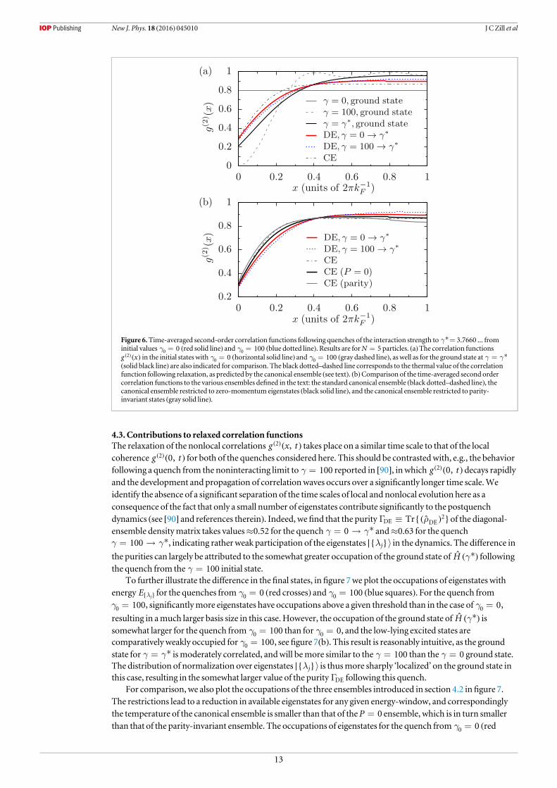
Infigure 6(a)weplot the second-order correlation function ( ) { ˆ ˆ ( )}( ) ( )r=g x g xTr 0,CE

2CE

2 in the canonical

ensemble (black dotted–dashed line), alongwith the diagonal-ensemble predictions ( )( )g xDE

2 for the quenchesfrom g = 00 (red solid line) and from g = 1000 (blue dotted line). For comparisonwe also plot the correlationfunctions in the initial states with g = 00 (horizontal line), g = 1000 (gray dashed line), as well as the groundstate for *g g= (solid black line). For the quench from g = 00 , the time-averaged value ( )( )g 0

DE2 is smaller than

the corresponding thermal value ( )( )g 0CE

2 , consistent with the results of [84, 90, 112]. In fact ( )( )g xDE

2 is suppressed

below ( )( )g xCE

2 over a range of separations p´ -x k0.4 2 F1. Correspondingly, ( ) ( )( ) ( )>g x g x

DE2

CE2 at larger

separations x due to particle number andmomentum conservation. For the quench *g g= 100 , the

diagonal-ensemble coherence function ( )( )g xDE

2 is similar in shape to that of the quench from g = 00 . However, itis somewhat smaller at x=0, and correspondingly larger at large x. This indicates somememory of the initialstate preserved by the dynamics of the integrable Lieb–Liniger system [58, 85]. Despite these differences, on thewhole both functions ( )( )g x

DE2 are comparable to ( )( )g x

CE2 (see also [66]).We note, however, that they are also both

reasonably close to the ground state result for ( )( )g x2 at interaction strength *g (solid black line), although thelocal value ( )( )g 0

DE2 for both quenches ismuch closer to the thermal value than the ground state value.

Since the system is in its ground state before the quench for both g = 00 and g = 1000 , and the total

momentumoperator P commutes with theHamiltonian, the postquench states at *g only have support oneigenstates with totalmomentum P=0. Furthermore, the spatially structureless initial state at g = 00 impliesadditional parity-invariance ({ } { }l l= -j j ) in Bethe rapidity space for the postquench eigenstates [93–95].Thus an interesting question to ask is if we constructed a canonical densitymatrix(27) restricted toP=0 states,or one further restricted to parity-invariant states (which are a subset of the P=0 states), would these yieldbetter agreement with the diagonal ensemble predictions for the quenches?We have performed theseconstructions with the temperature in both casesfixed via the postquench energy in the sameway as for thecanonical ensemble, see equation (27) and the following text.

Infigure 6(b), we plot the resulting second-order correlation function ( ) { ˆ ˆ ( )}( ) ( )r=g x g xTr 0,CE

2CE

2 for thestandard canonical ensemble (black dotted–dashed line), as well as in the restricted P=0 ensemble (solid blackline), and the parity-invariant ensemble (solid gray line).We also include the diagonal-ensemble predictions

( )( )g xDE

2 for the quenches from g = 00 (red solid line) and from g = 1000 (blue dotted line). It can be seen that therestricted ensembles give results for the correlation function that are quite close to the standard canonicalensemble, and are no closer to the diagonal ensemble results.

12

New J. Phys. 18 (2016) 045010 J CZill et al

4.3. Contributions to relaxed correlation functionsThe relaxation of the nonlocal correlations ( )( )g x t,2 takes place on a similar time scale to that of the localcoherence ( )( )g t0,2 for both of the quenches considered here. This should be contrastedwith, e.g., the behaviorfollowing a quench from the noninteracting limit to g = 100 reported in [90], inwhich ( )( )g t0,2 decays rapidlyand the development and propagation of correlationwaves occurs over a significantly longer time scale.Weidentify the absence of a significant separation of the time scales of local and nonlocal evolution here as aconsequence of the fact that only a small number of eigenstates contribute significantly to the postquenchdynamics (see [90] and references therein). Indeed, wefind that the purity {( ˆ ) }rG º TrDE DE

2 of the diagonal-ensemble densitymatrix takes values≈0.52 for the quench *g g= 0 and≈0.63 for the quench

*g g= 100 , indicating rather weak participation of the eigenstates ∣{ }l ñj in the dynamics. The difference in

the purities can largely be attributed to the somewhat greater occupation of the ground state of ˆ ( )*gH followingthe quench from the g = 100 initial state.

To further illustrate the difference in thefinal states, infigure 7we plot the occupations of eigenstates withenergy { }lE

jfor the quenches from g = 00 (red crosses) and g = 1000 (blue squares). For the quench from

g = 1000 , significantlymore eigenstates have occupations above a given threshold than in the case of g = 00 ,

resulting in amuch larger basis size in this case. However, the occupation of the ground state of ˆ ( )*gH issomewhat larger for the quench from g = 1000 than for g = 00 , and the low-lying excited states arecomparatively weakly occupied for g = 1000 , see figure 7(b). This result is reasonably intuitive, as the groundstate for *g g= ismoderately correlated, andwill bemore similar to the g = 100 than the g = 0 ground state.The distribution of normalization over eigenstates ∣{ }l ñj is thusmore sharply ‘localized’ on the ground state inthis case, resulting in the somewhat larger value of the purity GDE following this quench.

For comparison, we also plot the occupations of the three ensembles introduced in section 4.2 infigure 7.The restrictions lead to a reduction in available eigenstates for any given energy-window, and correspondinglythe temperature of the canonical ensemble is smaller than that of theP=0 ensemble, which is in turn smallerthan that of the parity-invariant ensemble. The occupations of eigenstates for the quench from g = 00 (red

Figure 6.Time-averaged second-order correlation functions following quenches of the interaction strength to *g = 3.7660 ... frominitial values g = 00 (red solid line) and g = 1000 (blue dotted line). Results are forN=5 particles. (a)The correlation functions

( )( )g x2 in the initial states with g = 00 (horizontal solid line) and g = 1000 (gray dashed line), as well as for the ground state at *g g=(solid black line) are also indicated for comparison. The black dotted–dashed line corresponds to the thermal value of the correlationfunction following relaxation, as predicted by the canonical ensemble (see text). (b)Comparison of the time-averaged second ordercorrelation functions to the various ensembles defined in the text: the standard canonical ensemble (black dotted–dashed line), thecanonical ensemble restricted to zero-momentum eigenstates (black solid line), and the canonical ensemble restricted to parity-invariant states (gray solid line).

13

New J. Phys. 18 (2016) 045010 J CZill et al

crosses) and from g = 1000 (blue squares) are suggestive of power-law decay at high energies. For small energieson the other hand,figure 7(b) shows that the functional form is not incompatible with exponential decay.

5. Conclusions

Wehave described amethod to calculatematrix elements between eigenstates of the Lieb–Linigermodel of one-dimensional delta-interacting bosons. Thismethod is based on the coordinate Bethe ansatz, which generates acomplete set of energy eigenfunctions for anyfixed coupling strength. This allows us to obtain overlaps betweeneigenstates of differentHamiltonians, as well as expressions for correlation functions. By introducing periodicboundary conditions, we obtained expressions amenable to numerical evaluation.We applied ourmethodologyto the evaluation offirst-, second-, third-, and fourth-order correlation functions in the ground state of the Lieb–Linigermodel for various values of the interparticle interaction strength. Our results indicate that although thecorrelations of the system are in general distorted by the small system size, finite-size effects become increasinglyless significant with increasing interaction strength and decreasing spatial separation.

Out of equilibrium,we investigated the dynamics of relaxation after a quantumquench of the interparticleinteraction strength towards a nonthermal steady state. Starting from two different initial states, we quenched toa common final interaction strength *g chosen in such away that both postquench energies were the same.Ourcalculations reveal a similar relaxation process for the second-order coherence ( )( )g x t,2 for both initial states:the build-up of correlations on short interparticle distances and their propagation through the system as timeprogresses. The time-averaged second-order correlation functions in both cases disagreedwith the predictionfor thermal equilibrium andwere biased, relative to one another, towards their pre-quench forms—an intuitiveresult given the integrability of the system. In the future it would be interesting to study quenches fromotherinitial states with the samefinal energy to explore how thememory of the initial state ismanifest in differentsituations.

Althoughourmethod is restricted to small systemsizes due to computational complexity andhere only applied tofiveparticles out of equilibrium,wewere able toobtain thedynamical evolution aswell as time-averaged correlationfunctions tohighprecision. Finallywenote that the evaluationofmatrix elements of the Lieb–Linigermodelwith thismethod isnot restricted to real-valuedBethe rapidities, opening thedoor to investigating thenonequilibrium

Figure 7. (a)Populations ∣ ∣{ }lC 2j of eigenstates with energies { }lE j following quenches to *g = 3.7660 ... from g = 00 (red crosses)

and g = 1000 (blue squares). Note that the y-axis is plotted on a logarithmic scale. For the quench from g = 1000 , additionalnonparity-invariant states appear in degenerate, parity-conjugate pairs and since their contributions is identical, the points lie on topof each other. The black dotted linewithfilled black circles represents the populations ( ){ }b- lE Zexp CEj of eigenstates with energies

{ }lE j for the canonical ensemble. The gray linewith grayfilled circles, and the black dashed linewith empty black circles are thecorresponding results for theP=0 restricted ensemble, and the parity-restricted ensemble, respectively. (b) Low-energy part of (a).

14

New J. Phys. 18 (2016) 045010 J CZill et al

dynamics of attractively interacting systems (where the rapidities becomecomplex-valued) and that followingquenches frommore complex initial states.

Acknowledgments

Thisworkwas supported byARCDiscovery Project, GrantNo.DP110101047 (JCZ, TMW,KVK, andMJD).MJD acknowledges the support of the JILAVisiting Fellows program.

AppendixA. Basis-set truncation

TheHilbert space of the Lieb–Linigermodel is infinite dimensional, and therefore the sums inequations (22),(23),and(26)must be truncated for numerical purposes. Here, we provide details of thetruncation scheme for the two different initial states we considered in section 4, and explain howwe quantify theerror resulting from this truncation.

For the quench from g = 00 , the initial state ∣y ñ0 only has nonzero overlapwith eigenstates ∣{ }l ñj of ˆ ( )*gHthat are parity invariant (i.e., eigenstates for which { } { }l l= -j j ) and, a fortiori, have zero totalmomentumP[114]. The strongly correlated initial state of the quench from g = 1000 similarly has zero overlapwitheigenstates ∣{ }l ñj with nonzero totalmomentum, but in this case states contributing to ∣ ( )y ñt , and thus rDE,need not be parity-invariant in general. For g = 00 our results for the overlaps agreewith recently obtainedanalytical expressions [94, 95], which predict real positive overlaps, given the phase convention implicit inequation (2), for quenches to g > 0. For g = 1000 , wefind that the overlaps are still real, but are no longerrestricted to positive values.

We briefly summarize our procedure to determine the cutoff here—see appendix A of [90] for an extendeddiscussion for the case of parity-invariant states. It can be shown [2] that the solutions { }lj of the Betheequations (3) are in one-to-one correspondencewith the numbersmj that appear in equation (3). This allows usto uniquely label states by the set { }mj .Without loss of generality, we order the numbersmj such that

> > > >-m m m mN N1 2 1 , andwe only need consider states for which å =m 0j j , corresponding to zerototalmomentumP.We specialize hereafter to the caseN=5, which is the largestN for whichwe consider thedynamics in this article. The states can be grouped into families, labeled bym1.We have found empirically thatwithin each such family, the eigenstate ( )- -m m, 1, 0, 1,1 1 has the largest absolute overlap ∣ { }∣ ∣l yá ñj 0 with theinitial state, for both initial states we consider (g = 00 and g = 1000 ). Furthermore, this overlap is larger thanthat of themost significantly contributing eigenstate ( )+ - - -m m1, 1, 0, 1, 11 1 of the following family( +m 11 ).We therefore construct the basis by considering in turn each familym1 and including all states withinthat family for which the overlapwith the initial state exceeds our chosen threshold valueCmin. Eventually, forsome value ofm1, even the eigenstate ( )- -m m, 1, 0, 1,1 1 has overlapwith ∣y ñ0 smaller than the threshold, atwhich point all states thatmeet the threshold have been accounted for.

We note that the Lieb–Linigermodel has an infinite number of conserved charges [ ˆ ˆ ( )]( ) g =Q H, 0;m

=m 0, 1, 2 ,..., with eigenvalues given by ˆ ∣{ } ∣{ }( ) l l lñ = å ñ=Qm

j lN

lm

j1 . However, for a quench from g = 00

their expectation values in the diagonal ensemble ˆ ( )á ñQm

DE diverge for all even m 4 [94, 95]. Our numericalresults suggest that this is also the case for quenches from g > 00 (indeed, they diverge for almost all states but

eigenstates [121, 122]). For all odd valuesm, the expectation values of the corresponding conserved charges ˆ ( )Q

m

are identically zero for our initial states and quench protocol. Thus, the only nontrivial and regular conservedquantities are the particle number (m=0) and energy (m=2). As in [90], we quantify the saturation of thenormalization and energy sum rules by the sum-rule violations

∣ ∣

∣ ∣ ( ) ( )

{ }{ }

{ }{ }

å

å å l

D = -

D = -

ll

g g ll

=

N C

EE

C

1 ,

11

, A1l

N

l

2

2

1

2

j

j

j

j

0

respectively, where g gE0

is the exact postquench energy (equation (24)).We note that the calculation of time-dependent observables involves a double sumover { }lj , and is thereforemore numerically demanding than thecalculation of expectation values in theDE.Moreover, the calculation of the local coherence ( )( )g t0,2 ismuchless demanding than that of the full nonlocal ( )( )g x t,2 .We therefore use different thresholdsCmin, resulting indifferent basis sizes and sum-rule violations, in the calculation of ( )( )g t0,2 , ( )( )g x t,2 , and ( )( )g x

DE2 , as indicated

in table A1 .Wenote that the energy sum rule is in general less well satisfied than the normalization sum rule,due to the lµ -4 tail of the diagonal-ensemble distribution of eigenstates [90].Wefind also that both sum rulesare less well satisfied for the quench *g g= 100 , despite the truncation procedure described above resulting

15

New J. Phys. 18 (2016) 045010 J CZill et al

inmore thanfive times asmany basis states being employed in its solution than are used in thequench *g g= 0 .

For expectation values in theCE (equation (27)), we truncate the basis by retaining all states with energiesbelow some cutoff Ecut. The inverse temperatureβ is then chosen tominimize the energy sum-rule violationDE. The normalization sum rule is fulfilled by construction. Since all states (not only thosewith zeromomentum) contribute to this sum, the number of eigenstates involved in canonical-ensemble calculations ismuch larger than that in diagonal-ensemble calculations. For the canonical-ensemble correlation functionplotted infigure 6we used an energy cutoff of ´ k3.2 102

F2, which yields a basis of ´2.1 106 eigenstates ∣{ }l ñj .

We checked that this cutoff is sufficiently large to ensure saturation of ( )( )g xCE

2 (figure 6). For the ensemble

restricted toP=0 eigenstates (figure 6(b)), we used an energy cut-off of ´ k6.4 105F2, corresponding to 44 530

eigenstates, while for the parity-invariant ensemblewe used an energy cut-off of ´ k8.5 106F2, corresponding to

64 204 eigenstates.

Appendix B. Time-averaged correlation functions and the diagonal ensemble

The time-averaged expectation value (equation (25)) of an operator O can be expressed as an expectation

{ˆ ˆ}r=O OTr in the time-averaged densitymatrix

ˆ ∣ ( ) ( )∣

∣ ∣ ∣{ } { }∣ ∣{ } { }∣ ( ){ }

{ }{ } { }

{ } { }{ } { }*

òå å

rt

y y

l l d l l

º ñá

= ñá + ñá ¢t

t

ll

l ll l

¥

¹ ¢¢l l¢

t t t

C C C

lim1

d

. B1j j E E j j

0

2,

j

j

j j

j j j j

Thefirst term in equation (B1) is simply the diagonal-ensemble densitymatrix rDE (equation (26)), to which rreduces in the absence of degeneracies in the spectrumof ˆ ( )gH . This is the case for the quench from g = 00 , as

the only eigenstates of ˆ ( )*gH with nonvanishing overlapswith ∣y ñ0 in this case are the parity-invariant states∣{ }l ñj with { }lj ={ }l- j , which are nondegenerate (see [90] and references therein). By contrast, in a quenchfrom g > 00 , ∣ ( )y ñt has support on nonparity-invariant states ∣{ }l ñj , which are degenerate with their parityconjugates ∣{ }l- ñj .

In general such degeneracies can have observable consequences for time-averaged expectation values [117].However, as can be seen from figure B1 , the correction to ( )( )g x

DE2 due to the contributions of degenerate

eigenstates in the case of the quench from g = 1000 is small. It is straightforward to show that the elements

{ }∣ ˆ ( )∣{ }( )l lá - ñg 0j j2 of the local second-order coherence between parity-conjugate statesmust vanish due to

symmetry considerations. At larger separations x, thematrix elements between these pairs of states are nonzero,as illustrated infigure B1(a). However, these contributions are small compared to the diagonal-ensemble result

( )( )g xDE

2 , and indeed the total contribution of all parity-conjugate states in ourfinite-basis description

(figure B1(b))would yield a barely visible correction to the function ( )( )g xDE

2 plotted infigure 6.We note also that

the substitution of rDE for the time-averaged densitymatrix r introduces negligible error in the calculation ofthe purity of thismatrix (section 4.3).

Table A1.Basis-set sizes and sum-rule violations for full nonlocal, time-evolving sec-ond-order coherence ( )( )g x t,2 , for local, time-evolving second-order coherence

( )( ) =g x t0,2 , and for time-averaged second-order coherence ( )( )g xDE2 following quen-

ches from g = 00 , and g = 1000 to *g = 3.7660 ....

g0 Typea Cmin No. states DN DE kF2

0 ( )( )g x t,2 ´ -5 10 5 673 ´ -7 10 7 ´ -6 10 3

0 ( )( )g t0,2 ´ -1 10 5 1704 ´ -7 10 8 ´ -3 10 3

0 ( )( )g xDE2 ´ -1 10 6 6282 ´ -2 10 9 ´ -8 10 4

100 ( )( )g x t,2 ´ -5 10 5 3704 ´ -4 10 6 ´ -4 10 2

100 ( )( )g t0,2 ´ -1 10 5 10473 ´ -5 10 7 ´ -3 10 2

100 ( )( )g xDE2 ´ -1 10 6 43918 ´ -2 10 8 ´ -2 10 3

a Occupations of the ( )( )g xDE2 basis set are used in the calculation of GDE (section 4.3).

16

New J. Phys. 18 (2016) 045010 J CZill et al

References[1] Lieb EHand LinigerW1963Phys. Rev. 130 1605–16

Lieb EH1963Phys. Rev. 130 1616–24[2] YangCNandYangCP 1969 J.Math. Phys. 10 1115[3] GirardeauM1960 J.Math. Phys. 1 516[4] Schultz TD 1963 J.Math. Phys. 4 666–71[5] LenardA 1964 J.Math. Phys. 5 930–43[6] VaidyaHG andTracyCA 1979Phys. Rev. Lett. 42 3–6[7] JimboMandMiwaT 1981Phys. Rev.D 24 3169–73[8] CreamerDB, ThackerH andWilkinsonD1986PhysicaD 20 155 – 186[9] ChernyAY andBrand J 2006Phys. Rev.A 73 023612[10] Forrester P J, FrankelNE andMakinM I 2006Phys. Rev.A 74 043614[11] Pitaevskii L and Stringari S 2003Bose–Einstein Condensation (Oxford:OxfordUniversity Press)[12] MoraC andCastin Y 2003Phys. Rev.A 67 053615[13] Haldane FDM1981Phys. Rev. Lett. 47 1840–3[14] Cardy J L 1984 J. Phys. A:Math. Gen. 17 L385[15] Berkovich A andMurthyG 1991 J. Phys. A:Math. Gen. 24 1537[16] CazalillaMA2004 J. Phys. B: At.Mol. Opt. Phys. 37 S1[17] KorepinVE, BogoliubovNMand Izergin AG1993Quantum Inverse ScatteringMethod andCorrelation Functions (Cambridge:

CambridgeUniversity Press)[18] Gangardt DMand ShlyapnikovGV2003Phys. Rev. Lett. 90 010401[19] Gangardt DMand ShlyapnikovGV2003New J. Phys. 5 79[20] CheianovVV, SmithH andZvonarevMB2006Phys. Rev.A 73 051604[21] OlshaniiM andDunjkoV 2003Phys. Rev. Lett. 91 090401[22] AstrakharchikGE andGiorgini S 2003Phys. Rev.A 68 031602[23] AstrakharchikGE andGiorgini S 2006 J. Phys. B: At.Mol. Opt. Phys. 39 S1[24] Schmidt B and FleischhauerM2007Phys. Rev.A 75 021601[25] Caux J S andCalabrese P 2006Phys. Rev.A 74 031605[26] Caux J S 2009 J.Math. Phys. 50 095214[27] PanfilM andCaux J S 2014Phys. Rev.A 89 033605[28] DrummondPD,Deuar P andKheruntsyan KV2004Phys. Rev. Lett. 92 040405[29] Deuar P, Sykes AG,Gangardt DM,DavisM J, DrummondPDandKheruntsyanKV2009Phys. Rev.A 79 043619[30] KormosM,MussardoG andTrombettoni A 2010Phys. Rev.A 81 043606[31] LenardA 1966 J.Math. Phys. 7 1268–72[32] Vignolo P andMinguzzi A 2013Phys. Rev. Lett. 110 020403[33] Sykes AG,Gangardt DM,DavisM J, VieringK, RaizenMGandKheruntsyanKV2008Phys. Rev. Lett. 100 160406[34] KheruntsyanKV,Gangardt DM,DrummondPDand ShlyapnikovGV2003Phys. Rev. Lett. 91 040403[35] Kinoshita T,Wenger T andWeissD S 2005Phys. Rev. Lett. 95 190406[36] Kinoshita T,Wenger T andWeissD S 2006Nature 440 900–3[37] Hofferberth S, Lesanovsky I, Fischer B, SchummTand Schmiedmayer J 2007Nature 449 324–7[38] GringM,KuhnertM, LangenT, KitagawaT, Rauer B, SchreitlM,Mazets I, Adu SmithD,Demler E and Schmiedmayer J 2012 Science

337 1318–22[39] Langen T,Geiger R, KuhnertM, Rauer B and Schmiedmayer J 2013Nat. Phys. 9 640[40] Haller E,GustavssonM,MarkM J, Danzl J G,Hart R, PupilloG andNägerlHC2009 Science 325 1224–7[41] Fabbri N, PanfilM, ClémentD, Fallani L, InguscioM, Fort C andCaux J S 2015Phys. Rev.A 91 043617[42] Guarrera V,MuthD, Labouvie R, Vogler A, Barontini G, FleischhauerMandOttH2012 Phys. Rev.A 86 021601[43] Vogler A, Labouvie R, Stubenrauch F, Barontini G,Guarrera V andOttH 2013Phys. Rev.A 88 031603[44] ClémentD, FabbriN, Fallani L, Fort C and InguscioM2009Phys. Rev. Lett. 102 155301[45] Paredes B,Widera A,MurgV,MandelO, Fölling S, Cirac I, ShlyapnikovGV,Hänsch TWandBloch I 2004Nature 429 277–81[46] vanAmerongenAH, van Es J J P,Wicke P, KheruntsyanKV and vanDrutenN J 2008Phys. Rev. Lett. 100 090402[47] Armijo J, Jacqmin T, KheruntsyanKV andBouchoule I 2010Phys. Rev. Lett. 105 230402[48] Armijo J, Jacqmin T, KheruntsyanK andBouchoule I 2011Phys. Rev.A 83 021605[49] Jacqmin T, Armijo J, Berrada T, KheruntsyanKV andBouchoule I 2011Phys. Rev. Lett. 106 230405[50] Meinert F, PanfilM,MarkM J, Lauber K, Caux J S andNägerl HC 2015Phys. Rev. Lett. 115 085301

Figure B1.Contributions of degenerate energy eigenstates to the time-averaged second-order correlation function following a quenchfrom g = 1000 to *g = 3.7660 ... forN=5 particles. (a)Contributions { }∣ ˆ ( )∣{ }{ } { }

( )* l lá - ñ +l l-C C g x0, c.c.j j2

j jof off-diagonal

matrix elements corresponding to the three largest weights { } { }*l l-C Cj j

. (b)Total contribution of degenerate energy eigenstates.

17

New J. Phys. 18 (2016) 045010 J CZill et al

[51] BermanGP, Borgonovi F, Izrailev FMand Smerzi A 2004Phys. Rev. Lett. 92 030404[52] Flassig D, Pritzel A andWintergerst N 2013Phys. Rev.D 87 084007[53] Dvali G, FlassigD,GomezC, Pritzel A andWintergerst N 2013Phys. Rev.D 88 124041[54] Kanamoto R, SaitoH andUedaM2003Phys. Rev.A 67 013608[55] Kanamoto R, SaitoH andUedaM2006Phys. Rev.A 73 033611[56] RigolM andMuramatsu A 2004Phys. Rev. Lett. 93 230404[57] RigolM,Muramatsu A andOlshaniiM2006Phys. Rev.A 74 053616[58] RigolM,DunjkoV, YurovskyV andOlshaniiM2007Phys. Rev. Lett. 98 050405[59] Cassidy AC,ClarkCWandRigolM2011Phys. Rev. Lett. 106 140405[60] GramschC andRigolM2012Phys. Rev.A 86 053615[61] HeK, Santos L F,Wright TMandRigolM2013Phys. Rev.A 87 063637[62] Wright TM,RigolM,DavisM J andKheruntsyanKV2014Phys. Rev. Lett. 113 050601[63] KormosM,ColluraMandCalabrese P 2014Phys. Rev.A 89 013609[64] Deuar P andDrummondPD2006 J. Phys. A:Math. Gen. 39 1163[65] Natu S S andMueller E J 2013Phys. Rev.A 87 053607[66] MuthD, Schmidt B and FleischhauerM2010New J. Phys. 12 083065[67] MuthD and FleischhauerM2010Phys. Rev. Lett. 105 150403[68] Gasenzer T, Berges J, SchmidtMGand SecoM2005Phys. Rev.A 72 063604[69] Berges J andGasenzer T 2007Phys. Rev.A 76 033604[70] Branschädel A andGasenzer T 2008 J. Phys. B: At.Mol. Opt. Phys. 41 135302[71] Gasenzer T andPawlowski JM2008Phys. Lett.B 670 135[72] Iucci A andCazalillaMA2009Phys. Rev.A 80 063619[73] ColluraM, Sotiriadis S andCalabrese P 2013Phys. Rev. Lett. 110 245301[74] ColluraM, Sotiriadis S andCalabrese P 2013 J. Stat.Mech.P09025[75] BuljanH, Pezer R andGasenzer T 2008Phys. Rev. Lett. 100 080406[76] JukićD, Pezer R, Gasenzer T andBuljanH2008Phys. Rev.A 78 053602[77] Pezer R,Gasenzer T andBuljanH 2009Phys. Rev.A 80 053616[78] GritsevV, Rostunov T andDemler E 2010 J. Stat.Mech.P05012[79] Sato J, Kanamoto R,Kaminishi E andDeguchi T 2012Phys. Rev. Lett. 108 110401[80] Mossel J andCaux J S 2010New J. Phys. 12 055028[81] IyerD andAndrei N 2012Phys. Rev. Lett. 109 115304[82] IyerD,GuanH andAndreiN 2013Phys. Rev.A 87 053628[83] Caux J S and Essler FHL 2013Phys. Rev. Lett. 110 257203[84] DeNardis J,Wouters B, BrockmannMandCaux J S 2014Phys. Rev.A 89 033601[85] MussardoG2013Phys. Rev. Lett. 111 100401[86] DeNardis J andCaux J S 2014 J. Stat.Mech.P12012[87] DeNardis J, Piroli L andCaux J S 2015 J. Phys. A:Math. Theor. 48 43FT01[88] Piroli L andCalabrese P 2015 J. Phys. A:Math. Theor. 48 454002[89] Caux J S, Calabrese P and SlavnovNA2007 J. Stat.Mech.P01008[90] Zill J C,Wright TM,KheruntsyanKV,Gasenzer T andDavisM J 2015Phys. Rev.A 91 023611[91] Dorlas TC 1993Commun.Math. Phys. 154 347–76[92] ArfkenGB andWeberH J 2005MathematicalMethods for Physicists (Cambridge: CambridgeUniversity Press)[93] BrockmannM,DeNardis J,Wouters B andCaux J S 2014 J. Phys. A:Math. Theor. 47 145003[94] BrockmannM2014 J. Stat.Mech.P05006[95] BrockmannM,Nardis J D,Wouters B andCaux J S 2014 J. Phys. A:Math. Theor. 47 345003[96] YurovskyVA,OlshaniiM andWeissD S 2008Adv. At.Mol. Phys. 55 61–138[97] CazalillaMA, CitroR, Giamarchi T,Orignac E andRigolM2011Rev.Mod. Phys. 83 1405–66[98] PenroseO andOnsager L 1956Phys. Rev. 104 576–84[99] YangCN1962Rev.Mod. Phys. 34 694–704[100] BarthMandZwergerW2011Ann. Phys., NY 326 2544–65[101] Tan S 2008Ann. Phys., NY 323 2952–70[102] WangMS,Huang JH, Lee CH, YinXG,GuanXWandBatchelorMT2013Phys. Rev.A 87 043634[103] KormosM,ChouYZ and Imambekov A 2011Phys. Rev. Lett. 107 230405[104] Tolra B L,O’HaraKM,Huckans JH, PhillipsWD, Rolston S L and Porto J V 2004Phys. Rev. Lett. 92 190401[105] Haller E, RabieM,MarkM J, Danzl JG,Hart R, Lauber K, Pupillo G andNägerl HC 2011Phys. Rev. Lett. 107 230404[106] ManningAG, RuGwayW,Hodgman S S,Dall RG, BaldwinKGHandTruscott AG 2013New J. Phys. 15 013042[107] Pozsgay B 2011 J. Stat.Mech.P11017[108] ChernyAY andBrand J 2009Phys. Rev.A 79 043607[109] XuWandRigolM2015Phys. Rev.A 92 063623[110] GolovachVN,Minguzzi A andGlazman L I 2009Phys. Rev.A 80 043611[111] Imambekov A andGlazman L I 2008Phys. Rev. Lett. 100 206805[112] KormosM, Shashi A, ChouYZ, Caux J S and Imambekov A 2013Phys. Rev.B 88 205131[113] Sotiriadis S andCalabrese P 2014 J. Stat.Mech.P07024[114] Calabrese P andDoussal P L 2014 J. Stat.Mech.P05004[115] ColluraM,KormosMandCalabrese P 2014 J. Stat.Mech.P01009[116] RigolM,DunjkoV andOlshaniiM2008Nature 452 854[117] Kaminishi E,Mori T, Ikeda TNandUedaM2015Nat. Phys. 11 1050[118] Deuar P and StobinskaM2013 arXiv:1310.1301[119] Imambekov A,Mazets I E, PetrovD S,GritsevV,Manz S,Hofferberth S, SchummT,Demler E and Schmiedmayer J 2009 Phys. Rev.A

80 033604[120] Mossel J andCaux J S 2012New J. Phys. 14 075006[121] Davies B 1990PhysicaA 167 433 – 456[122] Davies B andKorepinV 2011 arXiv:1109.6604

18

New J. Phys. 18 (2016) 045010 J CZill et al