paper - blind deconvolution through dsp

678 PROCEEDINGS OF THE IEEE, VOL. 63, NO. 4, APRIL 1975

Blind Deconvolution Through Digital Signal Processing

Invited Paper

A&rtmct-This paper m s the problem of deconvolving two sip- nrls when both are unknown. The authors call this problem blind d e convolution. The discussion develops two rehted solutions which can be apptied through digital signal processing in certain practial cues. The case of r e v h a t e d and resonated sound forms the center of the development. The specific problem of restoring old acoustic recordings provides an experimental test. The important effects of noise and nonstationary sign& lead to the detailed part of the presentation. In addition, the paper presents results for the case of images degraded by -me common forms of blur.

INTRODUCTION HE DECONVOLUTION problem (i.e., the problem of separating two signals that have been convolved) appears in many contexts. Several varied discussions occur in

this issue of the PROCEEDINGS alone [ 1 ]-[4]. For the pur- poses of this paper, it is important to distinguish two different forms of the problem. The first and simpler of these assumes that one of the two signals is known. ,The second assumes that both signals are unknown and, therefore, that the only data available is the convolution itself. We have come to call the task of estimating or eliminating one of the unknown signals blind deconvohtion.

Of course, as in any problem involving the separation of two signals, something must be known about the distinguishing characteristics of both signals for which blind deconvolution is to be carried out. In developing a solution it is desirable to keep these characteristics as nonspecific as possible. Broader applications are then available.

The distinguishing characteristics in this work are the signal extents. We assume that one signal is of considerably smaller extent than the other. Specifically, we mean that one of the signals may be significantly nonzero over a restricted domain the size of which is probably two decimal orders of magnitude or more smaller than the domain of the convolution. This situation happens frequently in practice when a long or continu- ing signal is degraded by a linear shift-invariant system. Rever- berated and resonated sound and certain blurred images are examples which we consider here.

It should be noted that the blind deconvolution problem as encountered in speech [ 1 I , [21 and seismic [ 31 signal processing is in conflict with the distinguishing characteristics just d e

Manuscript received October 10, 1974; revised November 9, 1974. This work was supported in part by the Advanced Research Rojects

C-0363. Agency of the Department of Defense unda Contract DAHC15-73-

Science Department, University of Utah, Salt Lake City, Utah 841 12. T. G. Stockham, Jr., and R. B. Ingebretsen are with the Computer

University of Utah, Salt Lake City, Utah. He is now with the T. M. Cannon was with the Computer Science Department of the

Los Alamos Scientific Laboratory, Los Alamos, N.Mex. 87544.

scribed because the durations of the signals involved tend to be comparable. However, some variance with this observation is presently the subject of research [ 5 1 .

Digital signal processing has been used to explore and imple- ment the methods we are presenting. The most important reason for using digital processing is that the complexity basic to the method is not presently within the scope of analog signal processing technology. Although this situation lowers cost and speed performance from what it might otherwise be, the method is much more practical in this respect than might be expected and is well within the reach of many classes of potential users.

An aspect of the digital processing method which often re- ceives too little attention is the requirement for converting ac- curately to and from digital data, respectively, before and after processing. When employing digital deconvolution, special attention must be paid to accuracy, because it is the nature of the deconvolution process to increase greatly the impact of small errors in the data. It is essential to reduce the effects of conversion inperfections to be below those of the noise in the original data. To do this requires care and effort. However, the basic methods are well understood [6J, [71 and the means for conveniently maintaining quality is available [ 8 1 .

Our approach to this work has been based heavily upon the interaction of theory and experiment. As a result, the discussion centers around reverberated and resonated sound. Our original interest involved blurred images. However, the two- dimensional aspect of and other detailed difficulties with that application, set us looking for one involving onedimensional signals. The problem we selected was that of restoring old recordings made by the acoustic method which was used until about the mid 1920’s. The problem seemed simple enough in theory and yet was practical and rich enough to provide a good test. Let us now place this problem in the context of blind deconvolution.

Contrary to the popular concept concerning old recordings, whether they be acoustic or electric, the problem of surface noise or scratch is not the most important. While this form of degradation is immediately obvious when playing any old recording, it is generally not the major difficulty that connois- sew listeners complain about, at least where collectorsquality copies are concerned. For acoustic recordings the major problem seems to be the resonant or reverberant characteristic given to the musical instruments or vocal sound by the primi- tive recording horns which were used to focus the sound energy onto the original wax disks. While it is well known that these acoustic mechanisms were incapable of transcribing frequencies much below 200 Hz or above 4000 Hz, these frequency limita- tions alone do not account for the degree of the degradation

STOCMAM e t al.: BLIND DECONVOLUTION 619

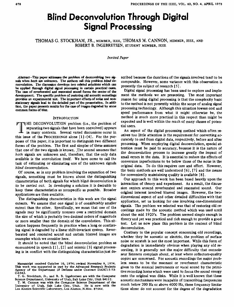
Fig. 1. A recording setup typical of those before the mid 1920’6.

produced. One can firmly convince oneself of this by taking a modem recording and passing it through sharp cutoff filters (digitally realized if one desires) with cutoff frequencies of the kind mentioned. One can even add some artificially generated surface noise if one wishes and still the listening quality will far exceed any available on old acoustic disks. Indeed, mea- surements made on old recording equipment indicate that sharp resonant amplitude distortions with variations from 10 to 20 dB or more are commonly encountered in the frequency range between 100 and 1000 Hz on such recordings. This effect not only produces a megaphone quality (which the reader might simulate by cupping his hands in front of his mouth and speaking) but also produces a very unpleasant effect in the form of loud bursts of sound when certain frequencies are played or sung.

Unfortunately, the amplitude distortions produced by acoustic recording equipment were not of fixed character from recording to recording. A typical setup, depicted in Fig. 1, involved five basic mechanisms (91. They were a horn for gathering acoustic energy, a tube for conducting that energy to a device called a sound box, a sound-boxdiaphram mechanism, a lever mechanism and associated stylus for cutting the groove, and a turntable driving a wax disk into which the recording was cut. As shown in the figure, the singing which ap- peared at the mouth of the recording horn as an acoustic signal s ( t ) was delivered to the disk after having been modified by the horn and its associated mechanism.

Surprisingly enough, the engineers of that day were excellent craftsmen and managed to avoid what we presently call nonlinear distortion quite well. The major effect of the recording horn system is, therefore, the same as that of a linear filter. In terms of functions, the singing waveform s ( t ) was convolved with the impulse response of the recording mechanism h ( t ) t o produce the recorded waveform u ( t ) . Except for surface noise, it is this latter waveform which is available to us today by playing an old recording.

Unfortunately, the recording horn impulse response h ( t ) was varied from one recording to another. The primary cause of this effect was probably due to the fact that the sound box mechanism played more the role of a resonant amplifier than that of an acoustic to mechanical transducer. The recording engineers knew this and were constantly making an effort to tune their sound boxes for maximum efficiency. Such tuning, coupled with the placement of recording horns, the length of connecting tubes, and the shape of the horns, provided marked variation in the characteristics of h ( t ) from recording to recording even for the same performer from day to day. Thus it is that in restoring these old recordings, we are faced with a blind deconvolution problem since we know neither the singing signal s ( t ) nor the impulse response h ( t ) involved in any particular recording under consideration.

L I

hlt) ; H (1)

n (1)

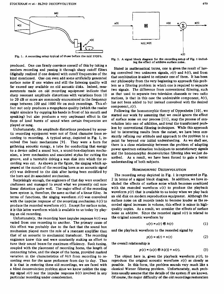
Fig. 2. A signal block diagram for the recording setup of FW. 1 includ- ing the effect of additive surface noise.

Stated in mathematical terms, one is given the result of having convolved two unknown signals, s ( t ) and h ( 0 , and from that combination is asked to estimate one of them. It has been our philosophy from the very beginning to approach this problem as a filtering problem in which one is required to separate two signals. The difference from conventional filtering, such as that used to separate two television channels or two radio stations, is that in this case the undesirable component, h ( t ) , has not been added to but instead convolved with the desired component, s ( t ) .

Following the homomorphic theory of Oppenheim [ 101, we started our work by assuming that we could ignore the effect of surface noise on our process [ 11 I , map the process of convolution into one of addition, and treat the transformed problem by conventional filtering techniques. While this approach led to interesting results from the outset, we have been constantly refining our attitude and approach to the problem to a point far beyond our initial understanding. As we shall see, there is a close relationship between the problem of adapting power spectrum estimation techniques to nonstationary signals and the homomorphic deconvolution filtering idea we just d e scribed. As a result, we have been forced to gain a better understanding of both subjects.

HOMOMORPHIC DECONVOLUTION The recording setup depicted in Fig. 1 is represented in Fig.

2 in terms of a signal block diagram. In addition, we have in- cluded the effects of surface noise which becomes combined with the recorded waveform u ( t ) to produce the playback waveform p ( t ) that is available to us today when we play back an old disk on modem reproduction equipment. Although the surface noise on all records tends to become louder as the r e corded signal increases in volume, this effect is minor in highquality copies. As a result, we consider the effects of surface noise as additive. Since the recorded signal u ( t ) is related to the original acoustic waveform by

u ( t ) = s ( t ) 0 h ( t ) (1)

and the playback waveform to the recorded signal by

A t ) = W ) + (2) the overall relatiodhip is

p ( t ) = ( s ( t ) 0 h ( t ) ) + no). The object here is, given the playback waveform p ( t ) , t o

reproduce the original acoustic waveform s ( t ) as closely as possible. In this form, the problem sounds very much like a classical Wiener filtering problem. Unfortunately, such problems usually assume that the details of the system H are known. Of course, the major difficulty of the old recordings restoration

680

problem is that the recording system frequency response H ( f ) is unknown. A second difference encountered here is that in classical filtering problems, the signals are assumed to be stationary. Acoustic waveforms of singing such as s ( t ) are far from stationary as can be readily appreciated by the fact that the energies in such signals possess strong variations from moment to moment.

Noting these issues and assuming for the time being that the noise n ( t ) is negligible, one is faced with the problem: given u ( t ) as in ( l ) , find s ( t ) . Following the homomorphic filtering concept, the first step in the process is to transform the convolution equation of (1) into a linear equation in the hope that the welldeveloped discipline of linear signal processing might be applied. This can be done by first taking the Fourier transform of both sides of ( l ) , thus producing

= S c f ) - H(f) (4 1 which is simply the familiar frequency response relationship between the input and the output spectra for a linear system. By further taking the complex logarithms of both sides of (4), we obtain

log V ( f l = log S(fl + log H c f ) ( 5 1 which possesses the additive property we wish.

At this juncture, one approach might be to take several recordings made with the same recording equipment, put each one in the form of (51, and average both sides of these equations across all of the recordings. If there were enough recordings and the singing on each were sufficiently different, one might expect, according to the central limit theorem, that the right-hand side of ( 5 ) would converge to log HV).

There are difficulties with this idea. The most important is that there are not a multiplicity of recordings available. There is only one, because h ( t ) was varied from one recording to another. This problem is overcome by chopping that recording into many intervals of moderate length (e.g., one-half-second intervals). Each of these intervals, which we will call ui(t), represents a slightly different musical passage perturbed by the same recording mechanism. A small difficulty arises, however. Each of these intervals is not given precisely as a convolution of the corresponding interval of the original acoustic wave and the impulse response of the recording horn. The problem d e tails have to do with edge effects at the ends of the chopped intervals. Nevertheless, if the intervals are long compared to the temporal extent of the impulse response h( t ) , the approximate relationship

ui ( t ) N si ( t ) 8 h ( t ) ( 6 )

results. Furthermore, by multiplying the chopped intervals by a

smooth window function, we obtain a slightly modified set of vi's which are related closely to the corresponding modified set of SI'S by

Ui(t) = Wi(t) * u ( t ) = Wi(t) - [ s ( t ) 0 h ( t ) ]

N [w i ( t ) * s ( t ) l 8 h ( t ) = si(t) 0 h ( t ) . (7)

If the windows wi(t) are smooth and long compared to the temporal extent of the impulse response h ( t ) , the approximate equality of (6) holds very closely. Taking the Fourier transform of both sides of (6) , we obtain

Vi (f) N Si (f) * H(fl. (8 )

PROCEEDINGS OF THE IEEE, APRIL 1975

Again, taking the complex logarithm, we obtain

If windows whose length is on the order of half-second are used and a 50-percent overlap from window to window is em- ployed (e.g., as is commonly done with a simple hanning window), and since a typical old recording might be between 3 and 5 min in duration, then from 300 to 600 intervals for which (9) holds would be available. Averaging over all of these intervals yields the relationship

We would at this point hope that the first term in the right- hand side of (10) would converge to zero for large' N . Un- fortunately, this does not happen. This fact is made clearer by writing (10) as two separate equations, the first equating the real parts and the second equating the imaginary parts of the complex quantities involved. This is done in

and

which descrii the approximate attenuation and phase rela- tionships between the original s i n g i n g and the recorded wave forms, respectively.

Concentrating first on the log amplitudes of (1 la), it would be our hope that the first term in the right-hand side would converge to zero for large N. Theoretical considerations would predict that this does not happen since, crudely speaking, this term represents in decibels the average distribution in frequency of the energies constituting musical signals. Practical experience bears out this expectation. Indeed, as we shall show shortly, if the singing waveform were a stationary process, this term would be one half of the logarithm of the power spectrum of that signal except for a small additive constant. It is common knowledge that even if one were to assume that a music waveform were stationary, its spectrum would be cer- tainly far from white (i.e., constant or flat). In pursuing the blind deconvolution objective, it remains to remove this term so that log IH(fll may be revealed.

This goal is reached by processing a modem recording of a musical selection similar t o the one to be restored in a manner identical to that just described. The recording mechanisms used to make the modem recordings, hereafter called proto- types, possess virtually flat frequency responses. For them, the second term in the right-hand side of (1 1) reduces to zero. Thus, for the modern recording, the averaging process yields an isolated version of the first term in the right-hand side of (1 1 a) which can then be removed by subtraction.' The basic

to the temporal extent of h(t) , is the essential motivation for the as- ' T h e requirement for large N, and that the windows be long compared

sumption made in the introduction that one unknown signal be of con- aidesably d e r extent than the other.

N. J. Miller who also selected the data and made th6 f i estimates that 'Claims for the subjective importance of this atep were fnst made by

were used.

STOCKHAM e? 01.: BLIND DECONVOLUTION 68 1

assumption of course is that the prototype recording has the same statistical characteristics as does the original singhg to be restored.

The problem with (1 lb) is not with the first term on the right-hand side converging to zero, but with the computation of phase in such a manner to be compatible with the equation itself. The issue, which is discussed thoroughly elsewhere [ l o ] , is that the four quadrant inverse tangent function con- ventionally used to compute phase yields only the principal value of the complex logarithm function. Unfortunately, the sum of principal value phases is not the principal value of a sum of phases. Thus the linearity which we require in (1 lb) cannot be obtained unless these phases are computed in a special way. One such method explored extensively by Schafer [ 121 relies on a process called phase unwrapping. However, we have so far been unable to apply phase unwrapping t o this problem. As a result, we have thus far not been able to estimate the phase distortions associated with old recordings. Since the human ear is known to be relatively insensitive to phase [ 131 , we have assumed the correction of phase distortions to be unnecessary. As we shall describe later, some experiments we have been able to perform indicate that this assumption is probably justified.

Returning our attention to the log amplitudes, we see that having computed the left-hand side of (1 la) for both the recording to be restored and the prototype, the next step is t o subtract the latter from the former leaving an estimate of log IH(f ) l . The remainder of the restoration process involves the construction of the compensating linear digital fiiter whose frequency response is the inverse of IH(f ) l . Of course, this approach is valid only under the strict assumption that the recording is noise free. In fact, such is not the case. Care is thus taken to confine the frequency response of the compensating filter to the frequency band in which the old recording has appreciable components. An attempt to recover frequencies outside this band would only serve to amplify surface noise un- duly without retrieving informative signals. This effect is formally known as ill-conditioning.

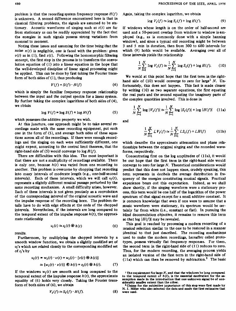
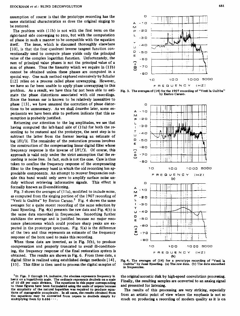
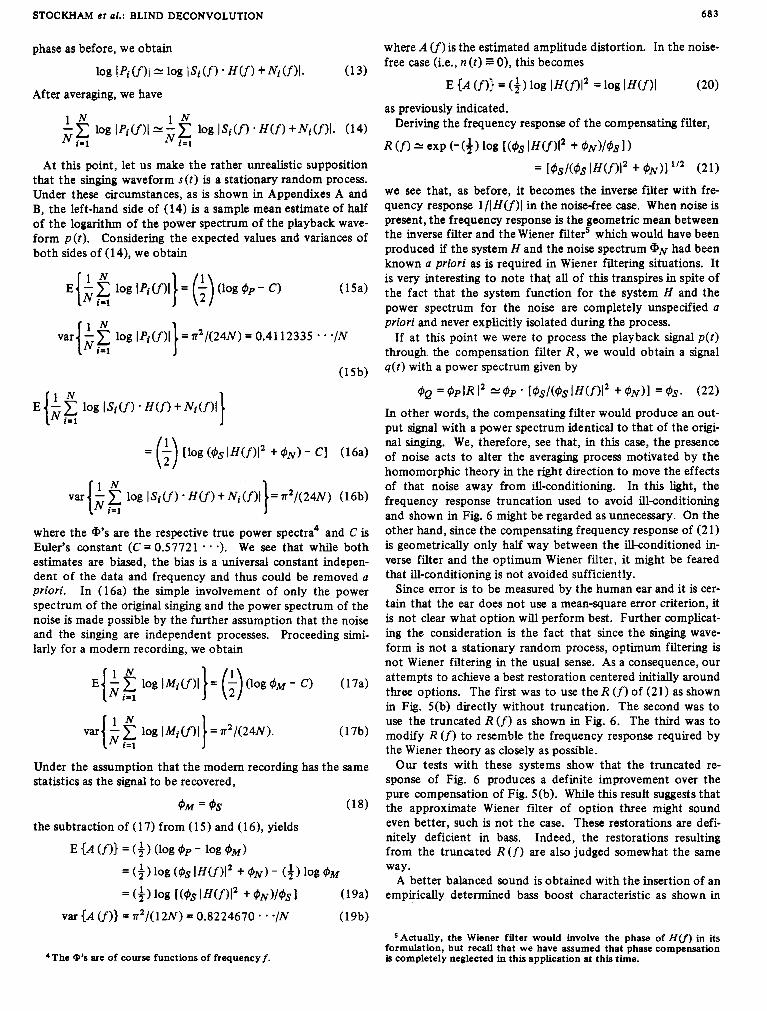
Fig. 3 shows the averages of (1 1 a), modified to include noise, as computed from the singing portion of the 1907 recording of “Vesti la Guibba” by Enrico car us^.^ Fig. 4 shows the same averages for a quite recent recording of the same selection by Jussi Bjoerling. Fig. 4(a) presents the raw data and Fig. 4(b) is the same data smoothed in frequencies. Smoothing further stabilizes the average and is justified because no major reso- nance phenomena which could produce sharp peaks are expected in the prototype spectrum. Fig. 5(a) is the difference of the two and thus represents an estimate of the frequency response of the horn used to make this recording.

When these data are inverted, as in Fig. 5(b), t o produce compensation and properly truncated to avoid ill-conditioning, the frequency response of the final restoration system is obtained. The results are shown in Fig. 6 . From these data, a digital filter is realized using established design methods [ 141 , [ 151. This filter is then used to process the digital samples of

0

A - 1 0 M p - 2 0 L I - 3 0

u -40

0 - 5 0

- 6 0 E

n d

-70

- 80 U

1 0 100 1 0 0 0 5000

F R E Q U E N C Y ( H Z 1

Fig. 3. The averages of (14) for the 1907 recording of “Vesti la Guibba” by Enrico Caruso.

0

A - 1 0 M p - 2 0 L I -30

1 0 1 0 0 1 0 0 0 5000

F R E Q U E N C Y [ H Z 1

(a) 0

A - 1 0 M -20

L I -30 T u - 4 0

0 E - 5 0

-60 d

U -70

-eo 1 0 1 0 0 1000 5000


(b) FIg. 4 . The averages of (14) for a prototype recording of “Vesti la

Guibba” by Jussi Bjoerling. (a) The raw data. (b) The data smoothed in frequencies.

In Figs. 3 through 14, inclusive, the abscissa represents frequency in the original acoustic disk by high-speed convolution processing. hertz on a logarithmic scale. The ordinate represents decibels on a scale ~ind~, the resulting samples are convert& to an =dog signal of 10 dB per main division. The equations in this paper corresponding to these fiiures have been formulated using the units of nepers because and presented for listening. the simplicity of the M t U d logarithm was required to produce qua- The results of this processing are very striking, especially tions of manageable complexity. In all cases, the results obtained from the rmry be from n e ~ s to decibels simply by from an artistic point of view where the emphasis is not so multiplying them by 8.686. - . much on producing a recording of modem quality as it is on

682 PROCEEDINGS OF THE IEEE, APRIL 1975

- 1 0 E

A - 2 0 .d.

U -30

- 4 0

1 0 100 1000 5000


(a) 4 0

A 30 M

p 20 L t 1 0 T u 00

- 1 0 E

cI -20 d e -30 U

- 4 0

I O 1 0 0 1000 5000

F R E GI U E N C Y [ H Z ]

@) Fig. 5 . The difference between the data of Figs. 3 and 4@). (a) Esti-

mate of amplitude distortions. @) Inverted data producing compensation frequency response.

4 0

A 30 M

p 2 0 L I 1 0 T u oo

- 1 0

- 2 0

- 3 0

- 4 0

E

d

U

1 0 1 0 0 1000 5000

F R E GI U E N C Y ( H Z 1

Fig. 6. The frequency response of Fig. 5(b) truncated to avoid ill- conditioning due to surface noise.

having a clear glimpse into past musical events. AU the restorations we have made, which so far concentrate on the recor,d- ings of Enrico Caruso, retain some of the “acoustic flavor” but the clarity of expression, the texture of the voice, and the artistic interest are dramatically changed. In addition, the prominent surges in volume caused when the pitch of the singing voice strikes the recording horn resonances are almost

entirely gone. The voice seems much closer to the listener, the megaphone sound having been almost completely eliminated. The realistic qualities of the voice provided by the upper range of frequencies within the range of the restoration process are dramatically obvious.

Restorations have been auditioned by a broad audience in- cluding laymen, musicians, and serious collectors of acoustic disks. A curious phenomenon has been revealed by the re- marks of the latter goup. Connoisseur collectors almost uni- formly agree that wheij $& acoustic recordings are played directly (i.e., without restoiiltion processing), they sound better on a wide range system rehoducing frequencies well above 3500 Hz. As we shall see, there is convincing evidence that no components of the original musical signal in this high-frequency band were recorded. Theories as t o why reproduction of this high band of the original should sound better center around the following arguments. It is better for the ear t o hear something in any band of frequencies than nothing at all. The surface noise which does extend into these frequencies is mod- ulated by the singing and thus provides a kind of artificial high- frequency structure. Small amounts of nonlinear distortion create harmonic components in these regions that enhance the listening experience. The curious phenomenon is that the restorations which we have produced contain no sensible energies in these frequency bands and yet are almost always judged superior to a highquality acoustic original reproduced in the simple wide-band manner.

At this point one might wonder whether the omission of phase compensation from the restoration procedure prevents it from realizing its full potential. While there is some hope that one might overcome the previously mentioned problems with computing the averages of (1 lb), no attempt has been made thus far. Instead, an experiment was performed to confirm the appropriateness of ignoring phase as a contributor to the audible defects associated with old acoustic disks. This experiment involves the computation of the minimum phase ass* ciated with the estimates of amplitude distortion. Starting with that estimate, Fig. S(b), the associated minimum phase is computed by means of a discrete Hilbert transform. That minimum phase is then combined with the truncated compensation frequency response of Fig. 6 . The auxiliary restoration h e a r filter thus formed is used to produce a restored sound. This restored sound is then compared with that obtained using zero phak as previously described. Careful auditioning on loudspeakers and earphones reveals no perceptible difference between these two restorations. The absence of such differences supports the assumption that the phases of (1 Ib) need not be estimated, provided the difference between the actual phase and the minimum phase is not too great. While it seems reasonable to ignore phase in restoring acoustic disks, this issue still remains unresolved and awaits further work.

THE EFFECTS OF NOISE From (4) through (1 Ib), we have neglected the effects of

surface noise upon the restoration of old recordings through blind deconvolution. If we attempt to rectify this, we obtain

pi (f) E H(f) + Ni (f) (12)

instead of (8). Here N i ( n is the Fourier transform of the ith- windowed noise segment. One can quickly see that taking the logarithm of both sides of (12) will now present some problems, because the right-hand side will not reduce to a sum of logarithms as is required. Proceeding anyway, and ignoring

STOCKHAM ef ai.: BLIND DECONVOLUTION 683

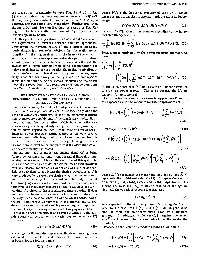
At this point, let us make the rather unrealistic supposition that the singing waveform s ( t ) is a stationary random process. Under these circumstances, as is shown in Appendixes A and B, the left-hand side of (14) is a sample mean estimate of half of the logarithm of the power spectrum of the playback waveform p ( t ) . Considering the expected values and variances of both sides of (14), we obtain

where the @'s are the respective true power spectra4 and C is Euler's constant (C = 0.57721 - * -). We see that while both estimates are biased, the bias is a universal constant independent of the data and frequency and thus could be removed u priori . In (1 6a) the simple involvement of only the power spectrum of the original singing and the power spectrum of the noise is made possible by the further assumption that the noise and the singing are independent processes. Proceeding similarly for a modem recording, we obtain

'The a's are of course functions of frequencyf.

where A (f) is the estimated amplitude distortion. In the noise- free case (i.e., n ( t ) 3 0), this becomes

E { A (f)) = (3) log IH(f)12 =log IH(f)l (20)

as previously indicated. Deriving the frequency response of the compensating filter,

R (f) = exp (-($I log [(@s I H U P + @N)/@Sl)

= [@s/(@S IH(f)I2 + @N)1 1'2 (21)

we see that, as before, it becomes the inverse filter with frequency response l/IH(f)l in the noise.-free case. When noise is present, the frequency response is the geometric mean between the inverse filter and the Wiener fiiter' which would have been produced if the system H and the noise spectrum @N had been known a priori as is required in Wiener filtering situations. It is very interesting to note that all of this transpires in spite of the fact that the system function for the system H and the power spectrum for the noise are completely unspecified u priori and never explicitly isolated during the process.

If at this point we were to process the playback signal p ( t ) through. the compensation filter R , we would obtain a signal q(t) with a power spectrum given by

@Q = $p IR 1' @P ' [@S/($S IH(f)lZ + @ N ) ] = @S. (22)

In other words, the compensating filter would produce an output signal with a power spectrum identical to that of the original singing. We, therefore, see that, in this case, the presence of noise acts to alter the averaging process motivated by the homomorphic theory in the right direction to move the effects of that noise away from ill-conditioning. In this light, the frequency response truncation used to avoid ill-conditioning and shown in Fig. 6 might be regarded as unnecessary. On the other hand, since the compensating frequency response of (21) is geometrically only half way between the ill-conditioned inverse filter and the optimum Wiener filter, it might be feared that ill-conditioning is not avoided sufficiently.

Since error is to be measured by the human ear and it is certain that the ear does not use a mean-square error criterion, it is not clear what option will perform best. Further complicat- ing the consideration is the fact that since the singing waveform is not a stationary random process, optimum filtering is not Wiener filtering in the usual sense. As a consequence, our attempts to achieve a best restoration centered initially around three options. The first was to use the R (f) of (21) as shown in Fig. 5(b) directly without truncation. The second was to use the truncated R ( f ) as shown in Fig. 6. The third was to modify R (f) to resemble the frequency response required by the Wiener theory as closely as possible. Our tests with these systems show that the truncated re-

sponse of Fig. 6 produces a definite improvement over the pure compensation of Fig. 5(b). While this result suggests that the approximate Wiener fiiter of option three might sound even better, such is not the case. These restorations are defi- nitely deficient in bass. Indeed, the restorations resulting from the truncated R ( f ) are also judged somewhat the same way.

A better balanced sound is obtained with the insertion of an empirically determined bass boost characteristic as shown in

formulation, but recall that we have assumed that phase compensation SActually, the Wiener filter would involve the phase of HCf) in its

is completely neglected in this application at this time.


4 0

M A 30

p 2 0

I 1 0 L

T u oo

- 1 0

- 2 0 E

n d 6 -30 U

- 4 0

1 0 1 0 0 1000 5000


Fig. 7. Empirically determined bass boost.

p 2 0 1 l , l ' 1 ! , . ,

L I 1 0 T u oo

- 1 0 E

n - 2 0 d B -30 U

- 4 0

1 0 1 0 0 1000 5000

F R E Q U E N C Y [ H Z ]

Fig. 8. T h e compensation frequency response of Fig. 6 with the bass boost of Fig. 7 added.

Fig. 7. The resulting restoration frequency response shown in Fig. 8 performs better than that shown in Fig. 6, although both achieve the major objective of alleviating the resonant and megaphone qualities of the original equally well. Compar- ison of Fig. 8 with inversions of frequency response curves published for old acoustic transducers, indicates a better match than the data of Fig. 6. Assuming that the published data are correct, calculations with (21) using measured surface noise energies and measured prototype spectra produce a frequency response which deviates from that of Fig. 6 especially in the bass region.

POWER SPECTRUM APPROACH Since (21) suggests the direct use of power spectra, our res-

toration scheme was modified to produce the compensation frequency response of (2 1) directly by power spectrum estimation techniques. In this approach the basic difference is that the averaging process performed after the taking of the logarithm in the homomorphic method is instead performed directly upon the squared magnitude of the Fourier transformed intervals of the playback signal. Starting again with (121, we obtain instead of (1 3)

of (14):

Following our desire to keep our results in terms of attenuation and to allow comparison with the homomorphic approach, we take the logarithm of both sides of (241, divide by two, and obtain

Retaining our supposition about the stationary nature of s ( t ) , as shown in Appendixes A and C, the left-hand side of (25) is a second sample mean estimate of half of the logarithm of the power spectrum of the playback waveform. Considering the expected values and variances of both sides of (251, we obtain

= $'(N)/4 = 1/(4N)

= $'(N)/4 = 1/(4N) (27b)

where $ (x) is the digamma function. Again, we have assumed that the surface noise and the singing are independent processes. For a modern recording, these same steps produce

(28b)

Again (18) holds and so the subtraction of (28) from (26) and Now after averaging, we have the following equation instead (27) leads to the same result as before expressed in (19)

STOCKHAM e2 al.: BLIND DECONVOLUTION 685

0

A -10 M

- 2 0 L I - 3 0 T u - 4 0

- 5 0 E

~ -60 d

-70 U

-80 I 1 , , : I

1 0 100 1000 5000


Fig. 9. The averages of (25) for the same C m s o recording as used to produce Fig. 3.

0

M A - I O

P - 2 0 L , - 3 0

T - 4 0

- 5 0 E

n d 8 -70

-60

U

- 80

1 0 1 0 0 1000 5000

F R E CJ U E N C Y [ H Z 1

(a) 0

M A - 1 0

p - 2 0 L I -30 T u - 4 0

- 5 0 E

~ -60 d e -70 u

- 80 1 0 1 0 0 1000 5000


(b) Fig. 10. The averages of (25) for the same Bjoerling recording used

to produce Fig. 4. (a) The raw data. (b) The data smoothed in frequencies.

through (22), except that (1 9b) becomes

v u { A (f)) = 1 / ( u v ) . ( 1 9 ~ )

In other words, these two system estimators are equivalent, (19), with the one based upon direct power spectrum estimates

M A 3 0

p 2 0

I 1 U

- 3 0

- 40 10 100 1000 5000

O - 1 0 E

~ - 2 0 d

U 6 - 3 0 1- -40 1 1 1 , , I

10 1 0 0 1000 5000


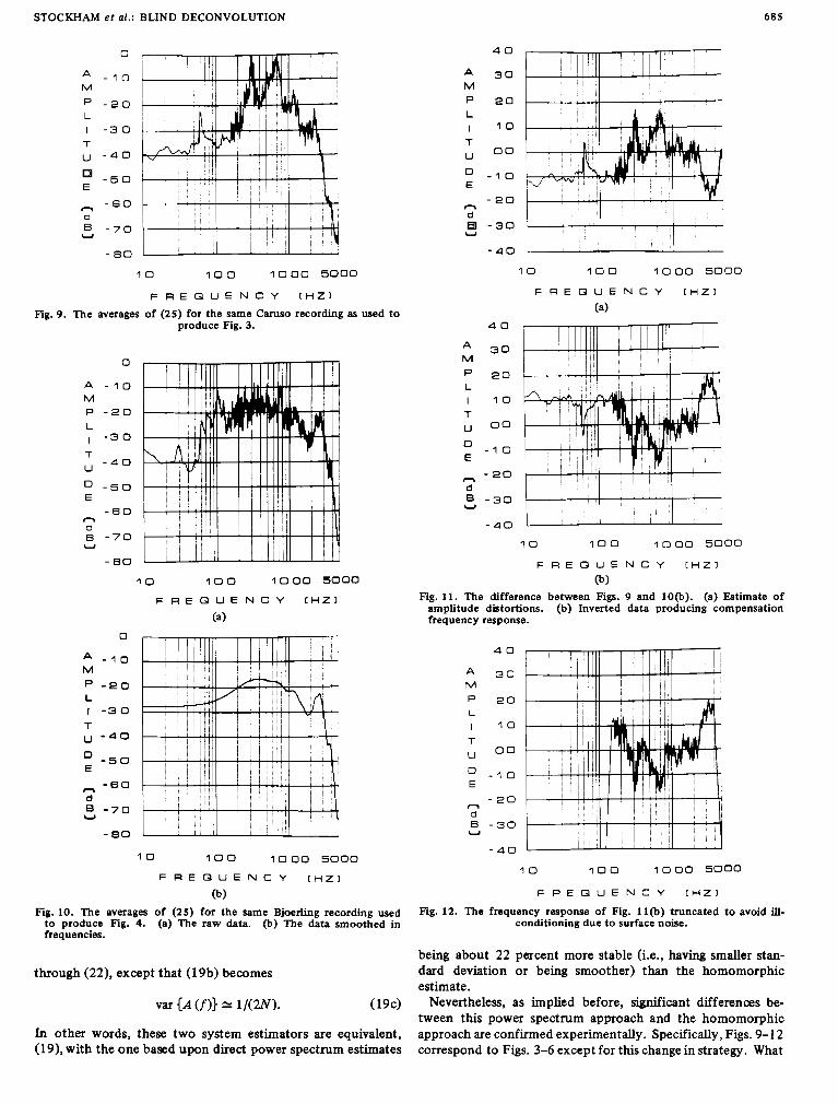
(b) Fig. 11. The difference between Figs. 9 and lo@). (a) Estimate of

amplitude distortions. (b) Inverted data producing compensation frequency response.

4 0

M A 30

p 2 0 L

I 1 0 T U O 0

-10 E

- 2 0 n d 8 - 3 0 U

- 4 0

10 100 1000 5000


Fig. 12. The frequency response of Fig. ll(b) truncated to avoid ill- conditioning due t o surface noise.

being about 22 percent more stable (i.e., having smaller standard deviation or being smoother) than the homomorphic estimate.

Nevertheless, as implied before, significant differences between this power spectrum approach and the homomorphic approach are confirmed experimentally. Specifically, Figs. 9-1 2 correspond to Figs. 3-6 except for this change in strategy. What


is more, notice the similarity between Figs. 8 and 12. In Fig. 12, the restoration frequency response agrees very closely with the empirically bass boosted homomorphic estimate. Also, upon listening, the two sound very much alike. Furthermore, even though (19b) and (19c) predict that the results of F i g . 5(a) ought to be less smooth than those of Fig. l l(a), just the reverse appears to be true.

At this point it is only natural to wonder about the cause of the experimental differences between the two approaches. Considering the physical nature of audio signals, especially music signals, it is somewhat obvious that the stationary assumption for the singing signal is at the heart of the issue. In addition, since the power spectrum estimates give more natural sounding results directly, a shadow of doubt is cast across the advisability of using homomorphic blind deconvolution for noisy signals inspite of its attractive theoretical motivation in the noise-free case. Somehow this makes no sense, especially since the homomorphic theory makes no assumptions about the stationarity of the signals involved and the power spectral approach does. As a result, let us set out to determine the effects of nonstationarity on both methods.

THE EFFECT OF NONSTATIONARY SIGNALS UPON HOMOMORPHIC VERSUS POWER SPECTRUM ESTIMATES OF

AMPLITUDE DISTORTIONS As is well known, the application of power spectrum estima-

tion techniques is permissible in the strict sense only when the signals involved are stationary. In addition, estimates involving time averages are possible only if the signals are ergodic. If, on the other hand, the time variations which characterize the nonstationary signals change slowly enough with time, power spectral estimates applied to such signals may still make sense. Since all power spectrum estimates used in this work involve averages over finite lengths of time, the requirement for this to be true is that the statistics of the signal change so slowly in each time interval to be analyzed that the estimation calculations are virtually unaffected. In this light, let us model the singing signal s ( t ) as being

formed by passing a stationary random signal through a time- varying linear system. Also let the variations of this system be so slow that we can consider the system to be time-invariant over any interval for which a Fourier analysis is to be applied. This is equivalent to modeling the singing waveform as if it were produced by a speech synthesis system such as commonly used in vocoders subject to the constraint that only unvoiced (i.e., hiss) [ 161 excitation to be used and that the parameters de- termining the frequency response of the vocal tract be slowly varying. Admittedly, this is a relatively simple model. It does not permit coherent components such as those produced by the very nearly periodic vibration of the vocal chords. None- theless, it has served us very well in this analysis and to produce a more sophisticated working model begins to approach the complexity of creating an automated singing music box.

Proceeding with this model and paying attention to the considerations with respect to slow variations and windows, (7) becomes

v t W = W t ) 0 b,<t) 0 h ( t ) (29)

where bt<t) is the impulse response of the slowly varying linear system during the ith interval. Taking the Fourier transform of both sides of (29), we obtain

K W = G , U ) * P X f l M f ) (30)

where &(fl is the frequency response of the slowly varying linear system during the ith interval. Adding noise as before, we get

PAfl= GAfl P A f l * H ( f l + NAfl (31)

instead of (12). Computing averages according to the homomorphic theory leads to

1 N - log IfKfll N ; log IGAfl P A f l * H(fl +NAfll. (32)

1 N

N i=1 i=1

Proceeding as motivated by the power spectrum approach, we have

It should be noted that (32) and (33) are no longer estimators of true log power spectra. This is so because the pi's are different for each interval.

In the noise-free case, as is shown in Appendixes D and E , the expected value and variances for these expressions are

(35b)

where L,(n represents the right-hand side of (32) and P,(fl represents the right-hand side of (33). Compare these equations with (16a), (16b), (27a), and (27b), respectively. As- suming no noise (is., @N = 0 ) and that all of the pi's are identical, the equations become identical, and

h

4 s = @G * 8'(fl (36)

as is expected in the stationary case. ^Permitting the pi's to vary, we see that both E {L,} and E {P,} will in general be modified from the stationary result, each by a different amoxnt. In addition, while var{Lp) remains the same, var {P,} is increased, the increase being larger the greater the variability.

Proceeding similarly for a modem recording, we obtain

STOCKHAM et al.: BLIND DECONVOLUTION 681

where a,{n is the frequency response of the slowly varying linear system during the ith interval of the prototype. The assumption that the prototype and the signal to be restored have the same statistics requires, for the homomorphic approach, that

( 3 9 4

and, for the power spectrum approach, that

For the assumption to hold simultaneously for both approaches, it is further required that the a’s and the 0’s be identical in pairs for each value of frequency f. However, the pairing need not be the same at all frequencies. If the prototype is the same musical selection, it would not be unreason- able to assume that

aI{f l= &(fl, i = 1,2, * * , N (40)

which is more than enough to guarantee (39a) and (39b).

and of (38) from (35) yields Under this assumption, the subtraction of (37) from (34)

E I’4(n}= (4) log I w 7 l 2 =log IH(nl (41 1 for both approaches, but

var {A,&-)} = nZ/( 12N) (424

for the homomorphic approach, and

for the power spectrum approach. Thus we see that while both attenuation estimates are un-

biased and equivalent, the one based upon the power spectrum approach is no longer guaranteed to be more stable. As a matter of fact, the greater .the dynamic range of the singing, the more unstable the power spectrum approach will be.

Assuming some reasonable variations for the &’s, we have shown both theoretically and experimentally that one obtains estimates which are about twice as stable using the homomorphic approach than using the power spectrum approach [171.

In practice, of course, the noise is not zero. Returning our attention to (32) and (33), we see, however, that due to the variation of the Pi’s there is no way to proceed as we did from (14) to (16a) and from (25) to (27a). The closest we can come is to regard the noise as a perturbation on each /3i(n and thus absorb it into (34a) and (35). The net effect would thus be to reduce the variations of the pi’s at frequencies for which the noise energy becomes large compared to the singing energies for an appreciable fraction of the time.

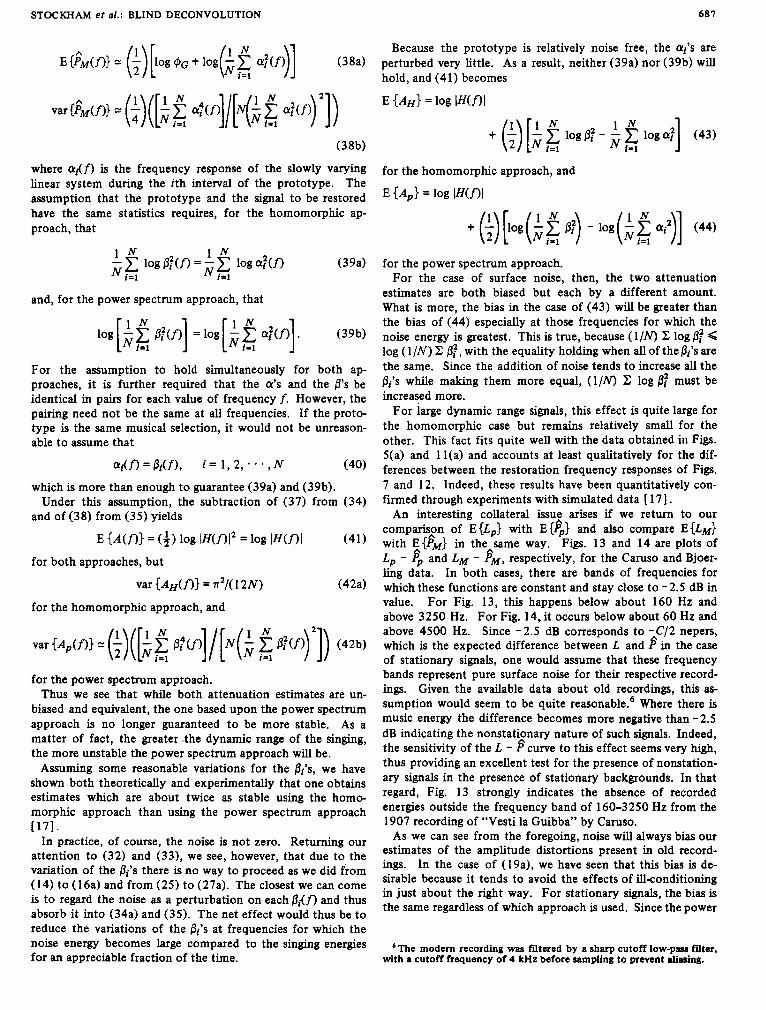
Because the prototype is relatively noise free, the ai’s are perturbed very little. As a result, neither (39a) nor (39b) will hold, and (41) becomes

E { A H } = log IWnl

for the homomorphic approach, and

for the power spectrum approach. For the case of surface noise, then, the two attenuation

estimates are both biased but each by a different amount. What is more, the bias in the case of (43) will be greater than the bias of (44) especially at those frequencies for which the noise energy is greatest. This is true, because (1/N) x log < log (1/N) Z Pi’, with the equality holding when all of the Pi’s are the same. Since the addition of noise tends to increase all the Pi’s while making them more equal, ( 1/N) 2 log 0: must be increased more.

For iarge dynamic range signals, this effect is quite large for the homomorphic case but remains relatively small for the other. This fact fits quite well with the data obtained in Figs. 5(a) and 1 l(a) and accounts at least qualitatively for the differences between the restoration frequency responses of Figs. 7 and 12. Indeed, these results have been quantitatively con- f i i e d through experiments with simulated data [ 171.

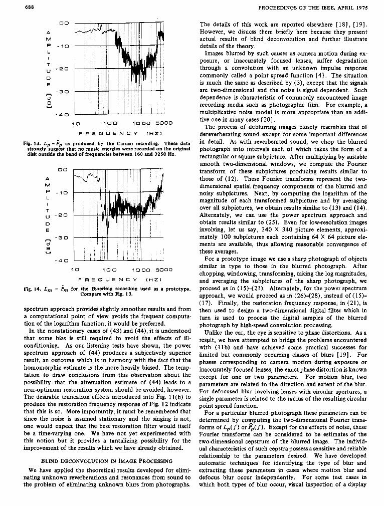
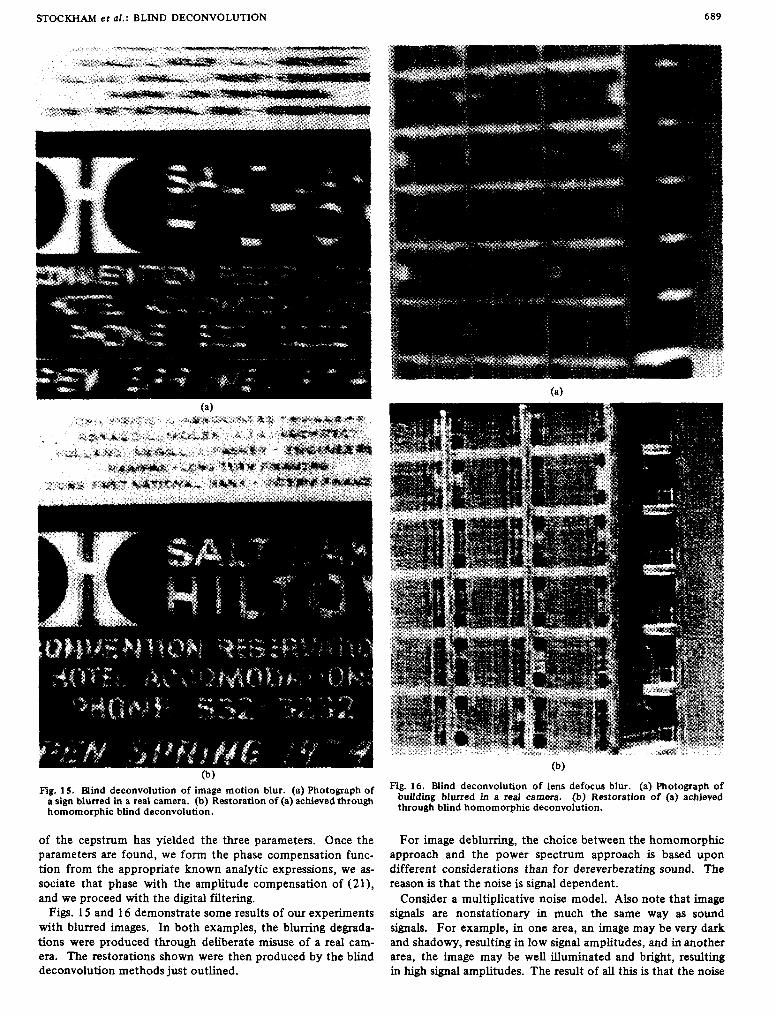
An interesting collateral issue arises if we return to our comparison of E{Lp} with E {4} and also compare E{LM} with E { f i ~ } in the Same way. Figs. 13 and 14 are plots of L, - 4 and LM - f i ~ , respectively, for the Caruso and Bjoer- ling data. In both cases, there are bands of frequencies for which these functions are constant and stay close to - 2.5 dB in value. For Fig. 13, this happens below about 160 Hz and above 3250 Hz. For Fig. 14, it occurs below about 60 Hz and above 4500 Hz. Since -2.5 dB corresponds to -C/2 nepers, which is the expected difference between L and f i in the case of stationary signals, one would assume that these frequency bands represent pure surface noise for their respective recordings. Given the available data about old recordings, this assumption would seem to be quite reasonable.6 Where there is music energy the difference becomes more negative than -2.5 dB indicating the nonstationary nature of such signals. Indeed, the sensitivity of the L - f i curve to this effect seems very high, thus providing an excellent test for the presence of nonstationary signals in the presence of stationary backgrounds. In that regard, Fig. 13 strongly indicates the absence of recorded energies outside the frequency band of 160-3250 Hz from the 1907 recording of “Vesti la Guibba” by Caruso.

As we can see from the foregoing, noise will always bias our estimates of the amplitude distortions present in old recordings. In the case of (19a), we have seen that this bias is desirable because it tends to avoid the effects of illconditioning in just about the right way. For stationary signals, the bias is the same regardless of which approach is used. Since the power

with a cutoff fiequency of 4 ItHz before sampling to prevent Iliasing. The modem recording was fdtered by a sharp cutoff low-paas Illter,


00

A M

p - 1 0 L I T

- 2 0

0 E

n

8 d

-3 0

U

- 4 0

1 0 1 0 0 1 0 00 5000


Fig. 13. L p - ip as produced by the Carum recording. These data strongly suggest that no music energies were recorded on the original disk outside the band of frequencies between 160 and 3250 Hz.

00

A M

p - 1 0 L I T " - 2 0 D E

~ -30 d B U

- 4 0

1 0 1 0 0 1000 5000


fig. 14. L, - P, for the Bjoerling recording used as a prototype. Compare with Fig. 13.

spectrum approach provides slightly smoother results and from a computational point of view avoids the frequent computation of the logarithm function, it would be preferred.

In the nonstationary cases of (43) and (44), it is understood that some bias is still required to avoid the effects of ill- conditioning. As our listening tests have shown, the power spectrum approach of (44) produces a subjectively superior result, an outcome which is in harmony with the fact that the homomorphic estimate is the more heavily biased. The temp- tation to draw conclusions from this observation about the possibility that the attenuation estimate of (44) leads to a near-optimum restoration system should be avoided, however. The desirable truncation effects introduced into Fig. 1 l(b) to produce the restoration frequency response of Fig. 12 indicate that this is so. More importantly, it must be remembered that since the noise is assumed stationary and the singing is not, one would expect that the best restoration filter would itself be a time-varying one. We have not yet experimented with this notion but it provides a tantalizing possibility for the improvement of the results which we have already obtained.

BLIND DECONVOLUTION IN IMAGE PROCESSING We have applied the theoretical results developed for elimi-

nating unknown reverberations and resonances from sound to the problem of eliminating unknown blurs from photographs.

The details of this work are reported elsewhere [ 181, [ 191. However, we disucss them briefly here because they present actual results of blind deconvolution and further illustrate details of the theory.

Images blurred by such causes as camera motion during exposure, or inaccurately focused lenses, suffer degradation through a convolution with an unknown impulse response commonly called a point spread function [4] . The situation is much the same as described by (3), except that the signals are two-dimensional and the noise is signal dependent. Such dependence is characteristic of commonly encountered image recording media such as photographic film. For example, a multiplicative noise model is more appropriate than an additive one in many cases [ 201.

The process of deblurring images closely resembles that of dereverberating sound except for some important differences in detail. As with reverberated sound, we chop the blurred photograph into intervals each of which takes the form of a rectangular or square subpicture. After multiplying by suitable smooth two-dimensional windows, we compute the Fourier transform of these subpictures producing results similar to those of (12). These Fourier transforms represent the two- dimensional spatial frequency components of the blurred and noisy subpictures. Next, by computing the logarithm of the magnitude of each transformed subpicture and by averaging over all subpictures, we obtain results similar to (1 3) and (14). Alternately, we can use the power spectrum approach and obtain results similar to (25). Even for low-resolution images involving, let us say, 340 X 340 picture elements, approximately 100 subpictures each containing 64 X 64 picture elements are available, thus allowing reasonable convergence of these averages.

For a prototype image we use a sharp photograph of objects similar in type to those in the blurred photograph. After chopping, windowing, transforming, taking the log magnitudes, and averaging the subpictures of the sharp photograph, we proceed as in (19421) . Alternately, for the power spectrum approach, we would proceed as in (26)-(28), instead of (1 5)- (17). Finally, the restoration frequency response, in (21), is then used to design a twodimensional digital filter which in turn is used to process the digital samples of the blurred photograph by high-speed convolution processing.

Unlike the ear, the eye is sensitive to phase distortions. As a result, we have attempted to bridge the problems encountered with (1 lb) and have achieved some practical successes for limited but commonly occurring classes of blurs [ 191. For phases corresponding to camera motion during exposure or inaccurately focused lenses, the exact phase distortion is known except for one or two parameters. For motion blur, two parameters are related to the direction and extent of the blur. For defocused blur involving lenses with circular apertures, a single parameter is related to the radius of the resulting circular point spread function.

For a particular blurred photograph these parameters can be determined by computing the two-dimensional Fourier transforms of Lp( f ) or 4( f ) . Except for the effects of noise, these Fourier transforms can be considered to be estimates of the two-dimensional cepstrum of the blurred image. The individ- ual characteristics of such cepstra possess a sensitive and reliable relationship to the parameters desired. We have developed automatic techniques for identifying the type of blur and extracting these parameters in cases where motion blur and defocus blur occur independently. For some test cases in which both types of blur occur, visual inspection of a display

STOCKHAM er al.: BLIND DECONVOLUTION 689

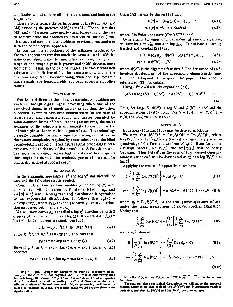
Fig. 15 . Blind deconvolution of image motion blur. (a) Photograph of a sign blurred in a real camera. (b) Restoration of (a) achieved through homomorphic blind deconvolution.

of the cepstrum has yielded the three parameters. Once the parameters are found, we form the phase compensation function from the appropriate known analytic expressions, we as- sociate that phase with the amplitude compensation of (21), and we proceed with the digital filtering.

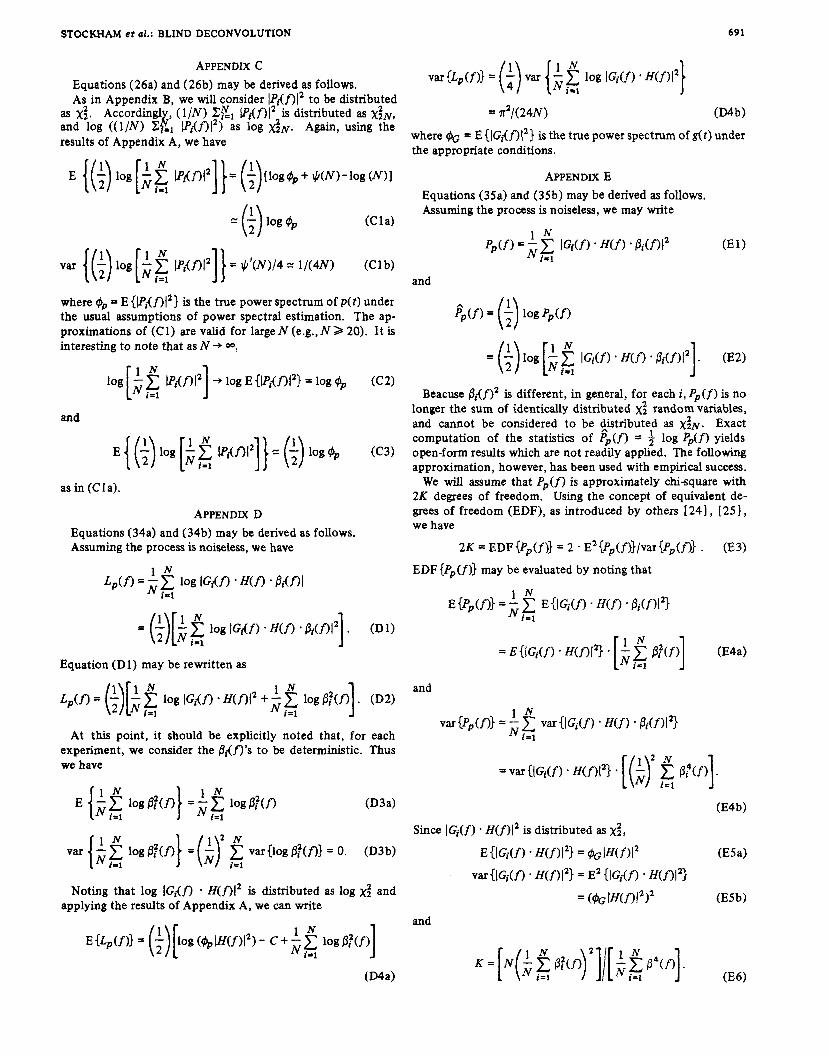
Figs. 15 and 16 demonstrate some results of o w experiments with blurred images. In both examples, the blurring degrada- tions were produced through deliberate misuse of a real camera. The restorations shown were then produced by the blind deconvolution methods just outlined.

Fig. 16. Blind deconvolution of lens defocus blur. (a) Photograph of bunding blurred in a real camera. (b). Restoration of (a) achieved through blind homomorphic deconvolutlon.

For image deblurring, the choice between the homomorphic approach and the power spectrum approach is based upon different considerations than for dereverberating sound. The reason is that the noise is signal dependent.

Consider a multiplicative noise model. Also note that image signals are nonstationary in much the same way as sound signals. For example, in one area, an image may be very dark and shadowy, resulting in low signal amplitudes, and in another area, the image may be well illuminated and bright, resulting in high s i g n a l amplitudes. The result of all this is that the noise


amplitudes will also be small in the dark areas and high in the Using (A3), it can be shown [ 181 that bright areas.

These effects reduce the perturbations of the pi's in (43) and (44) caused by the presence of Ni(f) in (31). The result is that (43) and (44) possess more nearly equal biases than in the case of additive noise and produce results closer to those of (1 9a). This fact reduces the bias problems previously encountered with the homomorphic approach.

In contrast, the smoothness of the estimates produced by the two approaches remains much the same as in the additive noise case. Specifically, for multiplicative noise, the dynamic range of the image signals is greater and (42b) deviates more from (1 9c). Thus, in the case of images, the two attenuation estimates are both biased by the same amount, and in the direction away from ill-conditioning, while for large dynamic range signals, the homomorphic approach provides smoother results.

CONCLUSIONS Practical solutions to the blind deconvolution problem are

available through digital signal processing when one of the convolved signals is of much greater extent than the other. Successful examples have been demonstrated for the cases of reverberated and resonated sound and images degraded by some common forms of blur. At the present time, the major weakness of the solutions is the inability to correct for the unknown phase distortions in the general case. The technology presently available for analog signal processing cannot realize the system complexity required by these solutions to the blind deconvolution problem. Thus digital signal processing is presently essential to the use of these methods. Although present- day signal processing involves higher costs and lower speeds than might be desired, the methods presented here can be practically applied at modest cost.'

APPENDIX A In the remaining appendixes, 2 and log 2 statistics will be

used and the following results needed. Consider, f i t , two random variables, y and z = log ( y ) with

y - d (x' with 2 degrees of freedom), E { y } = py , and var{y} = u$ = p$. Noting that a d distribution is equivalent to an exponential distribution, it follows that p y ( y ) = k * exp (-ky), where p y ( y ) is the probability density distribution associated withy and k = l/py.

We will now derive pz(z) (called a log 2 distribution with 2 degrees of freedom and denoted log d). Recall that z = f l y ) = log ( y ) . Under appropriate conditions [ 2 1 1,

PAZ) = Py(f-l(Z)) * I(d/dz)f-'(z)l. (AI)

Since df-'(z)/dz = f'(z) = exp (z), it follows that

p,(z) = k * exp (z - k exp (2)). (A21

Rewriting k as k = exp (-log (ilk)) = exp (-log py) , (A21 becomes

P&) = exp [z - log pY - exp (2 - log py)l. 643)

'Using a Digital Equipment Corporation PDP-10 computer, to ac- complish these restorations requires about 20 min of computing time for each image like those of Figs. 15 and 16 and about 2 h of computing

tributes a minor additional overhead. Digital proceasing facilitiea more time for a 4-min acoustic recording. A-D and D-A conversion con-

suited to production signal proceasing tasb would reduce these costs significantly.

E {z} = E {log ( y ) } = log p,, - C (A44

var{z} = n2/6 = 1.6449341 * - (A4b)

where Cis Euler's constant (C = 0.57721 e).

Generalizing for sums of independent random variables, we now let y - 2~ and z - log &. It has been shown by Bartlett and Kendall[22] that

E{z} = log py + $(N) - log ( N ) log py (A5a)

var {z} = $ '(N) = 1 /N (A5b)

where $(N) is the digamma function.' The derivation of (A5) involves development of the appropriate characteristic function and is beyond the scope of this paper. The reader is referred to [221 for details.

Using a Euler-Maclaurin expansion [23],

$(N)=log(N)- 1/(2N)- 1/(12W2+ l/(120N)4- * a * .

(A6)

Thus, for large N, $(N) + log N and $'(N) + 1/N and the approximations of (A5) hold. For N = 1, $(1) = -C, $'(1) = n2/6, and (A5) reduces to (A4).

APPENDIX B Equations (1 5a) and (1 5b) may be derived as follows. We note that Pi<f)12 = Re{Pi<f)}' + Im{Pi(f)}2, where

Re{Pi<f)} and Im{&f)} are the real and imaginary parts, respectively, of the Fourier transform of pi ( t ) . Even for a non- Gaussian process, Re {e{f)} and Im{Pi(f)} will be nearly Gaussian. Thus Pi<f)12, as the sum of two squared Gaussian random variables: will be distributed as d and log & ( f ) 1 2 as log d .

Applying the results of Appendix A, we have

var{ '2 log&(f)12} =n2/6N= 1.6449341 - * - / N (Blb) N i=1

where #p = E{Pt{f)12} is the true power spectrum of p ( t ) under the usual assumptions of power spectral estimation. Noting that

we have, as desired,

Note that J, (r) = d log r(t)/dt and r(r) = Gx" ' e -x dx is the gamma function.

mating assumption that each of the kiu>12's are independent random 9Throughout these statistical discussions we wiU make the approxi-

variables, and that Re (.&f)} and Im {Ptiu>} are uncorrelated.

STOCKHAM cr al.: BLIND DECONVOLUTION 69 1

APPENDIX C v u { t , ( f ) ) = (i) var { 2 log IGi(f) * ~ ( f ) 1 2 }

1 N Equations (26a) and (26b) may be derived as follows. As in Appendix B, we will consider IPiffl12 to be distributed

as X:. Accordingl , ( 1 /N) Zgl C P i ( f ) l ' is distributed as X ~ N , and log (( l /N) CZz1 1 p z & f l 1 2 ) as log 2 ~ . Again, using the results of Appendix A, we have

K = nZ/(24N) (Wb)

where q 5 ~ = E{IG&fll'} is the true power spectrum of g(f) under the appropriate conditions.

E { (:) log [f $ IPxfll']}= (:)(log$+ $(N)-log(N)I APPENDIX E Equations (35a) and (35b) may be derived as follows. Assuming the process is noiseless, we may write

= (;) 1% $ (C 1 a) 1 N

N i = l p p ~ ) = - IGi(f) * ~ ( f ) Pi(n12 (El)

vu { (:) log [ f 2 Pt091'] / = $'(N)/4 zz 1/(4N) (C1 b) and

where 6 = E { l P t & f l 1 2 } is the true power spectrum of p ( f ) under the usual assumptions of power spectral estimation. The approximations of (Cl) are valid for largeN(e.g., N > , 20). I t is interesting to note that as N -P 00,

and

as in (Cla).

APPENDIX D Equations (34a) and (34b) may be derived as follows. Assuming the process is noiseless, we have

1 N &(fl = ; log Icz&n * H(fl * P t & f l l

i=l

Equation (Dl) may be rewritten as

Beacuse &(f)' is different, in general, for each i, P p ( f ) is no longer the sum of identically distributed x: random variables, and cannot be considered to be tistributed as Exact computation of the statistics of P p ( f ) = 3 log Pp(n yields

(C3) open-form results which are not readily applied. The following approximation, however, has been used with empirical success.

We will assume that Pp(n is approximately chisquare with 2K degrees of freedom. Using the concept of equivalent degrees of freedom (EDF), as introduced by others [ 241, [25], we have

2K = EDF{Pp(f)) = 2 . E2{Pp(f)}/var{Pp(f)) . (E31

EDF{Pp(f)} may be evaluated by noting that

At this point, it should be explicitly noted that, for each experiment, we consider the pi<f)'s to be deterministic. Thus we have

Noting that log IG&fl H(fl1' is distributed as log x; and applying the results of Appendix A, we can write

and

692 PROCEEDINGS O F THE IEEE, APRIL 1975

Note that if a l l the &(f)’s are identical, then (E6) becomes K = N as expected for a stationary process.

Using this approximation with the results of Appendix A, we have, as desired,

var{iiP(f)} - $’(K) 2: 1/(4K) ( 3

where the last terms in each equation are valid for large N .

ACKNOWLEDGMENT

The authors wish to thank the people who have helped along the course of research leading to the ideas presented here. They are grateful for the contributions of G. Randall, R. B. Warnock, M. Milochik, K. Gerber, N. J. Miller, R. Rom, E. Ferretti, and many others who have given encouragement, interest, criticism, and ideas. Special thanks are due D. W. Evans of Salt Lake City, Utah, for the acoustic restoration idea, and S. B. Fassett of Boston, Mass., for his deep insight into and interest in the technical, musical, and historic aspects of acoustic recordings.

REFERENCES J. Makhoul, “Linear prediction: A tutorial review,” this issue, pp.

R. W. Schafer and L. R. Rabiner, “Digital representations of speech signals,” this issue, pp. 662-677. L. C. Wood and S. Treitel, “Seismic signal processing,” this issue, pp. 649661. B. R. Hunt, “Digital image processing,” this issue, pp. 693-708.

561-580.

[ 5 1 R. B. Smith and R. M. Otis, “Homomorphic deconvolution by log spectral averaging,” submitted for publication to Geophysics.

[ 6 ] T. G. Stockham, Jr., “A-D and D-A converters: Their effect on digital audio fidelity,” in DiB’ral Signal Processing, L. R. Rabiner and C. M. Rader, Eds. New York: IEEE Press, 1972, pp.

[7 ] S. Kriz, “A 16-bit A-D-A conversion system for high fidelity audio research,” in Proc. ZEEE Symp. Speech Recognition, pp.

[8 ] C.-M. Tsai, “A digital technique for testing A-D and D A con- 278-282, Apr. 1974.

verters,” M.S. thesis, Univ. Utah, Salt Lake City, June 1973. [9 ] 0. Read and W. L. Welch, From Tin Foil to Stereo. Indianapolis,

[ lo ] A. V. Oppenheim, R. W. Schafer, and T. G. Stockham, Jr., “Non- Ind.: Howard W. Sams, 1959.

linear fdtering of multiplied and convolved signals,” h o c . ZEEE,

[ 11 ] M. Medress, “Noise analysis of a homomorphic automatic volume control,” S.M. thesis, Dep. Elec. Eng., M.I.T., Cambridge, Mass.,

[ 121 R. W. Schafer, ‘‘Echo removal by discrete generalized linear Jan. 1968.

fdtering,” Tech. Rep. 466, M.I.T. Res. Lab. Electron.,Cambridge, Mass., Feb. 1969.

[ 131 J. L. Goldstein, “Auditory spectral fdtering and monaural phase perception,” J. Acoust. Soc. Amer., vol. 41, no. 2, pp. 458-479,

[ 141 B. Gold and C. M. Rader, Digital ProcesPing of Signals. New 1967.

[ 1 5 ] H. D. Helms, “Nonrecursive digital fdters: Design methods for York: McGraw-Hill, 1969, pp. 203-232.

achieving specifications on frequency response,” ZEEE Trans.

[ 161 J. L. Flanapn, Speech Analysis Synthesis and Perception, 2nd Audio Elecrroacoust., vol. AU-16, pp. 336-342, Sept. 1968.

Ed. New York: Springer-Verlag, 1972, pp. 321-395. [ 171 R. B. Ingebretsen, “Log spectral estimation for stationary and

Utah, Salt Lake City, 1975. nonstationary processes,’’ M.S. thesis, Comput. Sci. Dep., Univ.

[ 181 E. R. Cde , “The removal of unfiown image blurs by homomorphic filtering,” Comput. Sci. Dep., Univ. Utah, Salt Lake City, UTECCSc-74-029, June 1973.

[ 191 T. M. Cannon, “Digital image deblurring by nonlinear homomorphic filtering,” Comput. Sci. Dep., Univ. Utah, Salt Lake City,

[20] J. F. Walkup and R. C. Choens, “Image processing in signal-

[ 2 11 E. Parzen, Modem Probability Theory and Its Applications. New dependent noise,” Opr. Eng., vol. 13, no. 3, May/June, 1974.

[22] M. S. Bartlett and D. G. Kendall, “The statistical analysis of York: Wdey, 1960, p. 312.

variance heterogeneity and the logarithmic transformation,” J . Res. Statist. Soc. (Suppl.),vol. 8, pp. 128-138, 1946.

[23] CRC Standard Mathematical Tables, 22nd ed., Samuel M. Selby, Ed. Cleveland, Ohio: CRC Press, 1973, p. 483. [24] R. B. Blackman and J. W. Tukey, The Measurement of Power

Spectra, New York: Dover,-1958, p. 22. (251 P. D. Welch, “The use of fast Fourier transform for the estimation

of power spectra: A method based on time averages over short, modified periodograms,” IEEE Trans. Audio Elecrroacousr., vol. AU-15, pp. 70-73, June 1967.

484-496.

VOl. 56, pp. 1264-1291, Aug. 1968.

UTECCSC-74-091, AUg. 1974.

paper - blind deconvolution through dsp

Documents