paper bf-140 using regression splines in sas stat...

1

Paper BF-140

Using Regression Splines in SAS® STAT Procedures Jonas V. Bilenas, Barclays PCB

Nish Herat, Verizon Wireless

ABSTRACT SAS® has a number of procedures for smoothing scatter plots. In this tutorial, we review the nonparametric technique called LOESS, which estimates local regression surfaces. We review the LOESS procedure and then compare it to a parametric regression methodology that employs restricted cubic splines to fit nonlinear patterns in the data. Finally we look at multivariate adaptive regression splines (MARS) models which utilize a non-parametric regression technique to find a relationship. Not only do these three methods fit scatterplot data, but they can also be used to fit multivariate relationships.

INTRODUCTION One of the goals in statistical modeling is identifying whether relationships between variables are random or have some functional form. Scatter plots are often used to evaluate if relationships exist between variables and to determine if the relationships are linear or not. Non-linear relationships can still be used in linear models after transformations of the dependent and/or the independent variables.

SAS offers a number of scatterplot smoothing methodologies. In this paper we will examine the LOESS methodology pioneered by Cleveland, Devlin, and Grosse (1988), Cleveland and Grosse (1991), and Cleveland, Grosse, and Shyu (1992). LOESS performs nonparametric local regression smoothing for estimating regression surfaces. Using the methodology does not require any assumptions about the parametric relationship between variables and is therefore a useful tool in data exploration.

To model non-linear relationships using parametric linear regression models will require data transformations, typically of the independent (or predictor) variables. We will look at transformation procedures called restricted cubic splines proposed by Stone and Koo (1985) and multivariate adaptive regression splines (MARS) from Friedman (1991). We compare results to the LOESS procedure which does not provide a mathematical functional formula for the relationship observed. In this paper we will look at a simple bivariate example but the methodologies do extend to more than 2 dimensions.

LOESS OUTPUT USING SGPLOT

LOESS fits a localized regression function to data within a chosen neighborhood of points. The radius of the neighborhood is determined by the percentage of the data used in each neighborhood. The percentage is specified in SAS as a smoothing parameter which ranges from 0 to 1. The larger the parameter specified, the smoother the nonparametric prediction. The methodology is resistant to outliers since the predicted fit is weighted by the distance of each point to the center of the neighborhood.

Let’s start by looking at an example of LOESS using the SGPLOT procedure. We will be using the SAS help data set named CARS for illustration purposes. For this example we would like to investigate the relationship between highway miles per gallon as a function of the rated horse power of each car in the data set. The SGPLOT has a LOESS statement that can add a line to the scatterplot that represents a LOESS fit. Code using SAS 9.2 is shown in program 1. Output from the code is illustrated in figure 1.

http://support.sas.com/documentation/cdl/en/statug/63033/HTML/default/statug_loess_sect034.htm



2

Program 1

%let DS=sashelp.cars; /*1*/

%let Y=MPG_Highway;

%let X=Horsepower;

options orientation=landscape; /*2*/

goptions reset=all display vsize=5in hsize=7in; /*3*/

ods rtf file ="LOESS_TESTING.doc" style=banker; /*4*/

ods graphics on / ANTIALIASMAX=21500; /*5*/

proc sgplot data=&DS.; /*6*/

LOESS Y=&Y. X=&X. / smooth=0.5; /*7*/

XAXIS grid; /*8*/

YAXIS grid;

title LOESS Fit;

title2 Using SGPLOT;

run;

ods graphics off; /*9*/

ods rtf close;

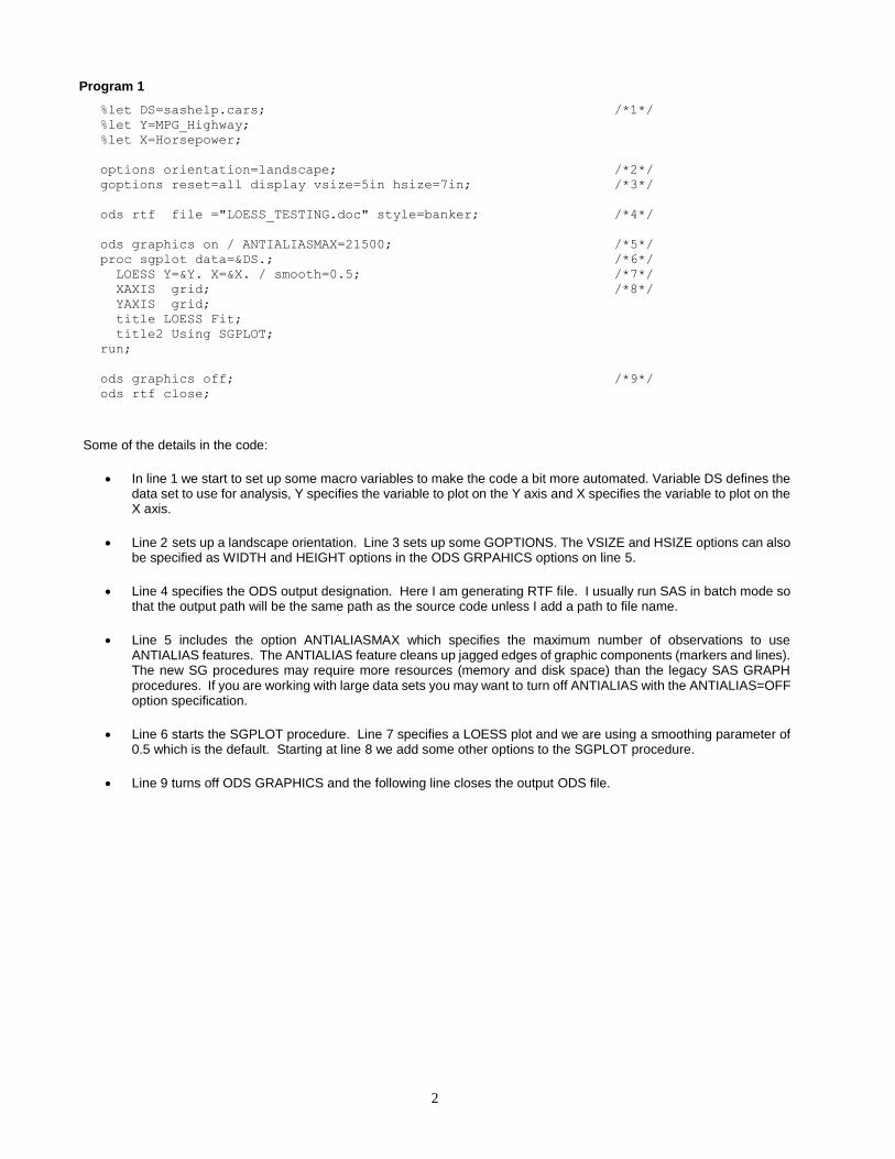
Some of the details in the code:

In line 1 we start to set up some macro variables to make the code a bit more automated. Variable DS defines the data set to use for analysis, Y specifies the variable to plot on the Y axis and X specifies the variable to plot on the X axis.

Line 2 sets up a landscape orientation. Line 3 sets up some GOPTIONS. The VSIZE and HSIZE options can also be specified as WIDTH and HEIGHT options in the ODS GRPAHICS options on line 5.

Line 4 specifies the ODS output designation. Here I am generating RTF file. I usually run SAS in batch mode so that the output path will be the same path as the source code unless I add a path to file name.

Line 5 includes the option ANTIALIASMAX which specifies the maximum number of observations to use ANTIALIAS features. The ANTIALIAS feature cleans up jagged edges of graphic components (markers and lines). The new SG procedures may require more resources (memory and disk space) than the legacy SAS GRAPH procedures. If you are working with large data sets you may want to turn off ANTIALIAS with the ANTIALIAS=OFF option specification.

Line 6 starts the SGPLOT procedure. Line 7 specifies a LOESS plot and we are using a smoothing parameter of 0.5 which is the default. Starting at line 8 we add some other options to the SGPLOT procedure.

Line 9 turns off ODS GRAPHICS and the following line closes the output ODS file.

3

Figure 1. LOESS Curve Generated by PROC SGPLOT

The relationship we see in figure 1 is definitely not linear. The slope gradually tapers off as the horsepower increases.

THE LOESS PROCEDURE SAS has the LOESS procedure which provides more options and features than what is available in the SGPLOT procedure to do local regression smoothing. Program 2 shows output using the same data used in program 1. You will need to have lines 1-5 from program 1 added before the PROC LOESS step. Output is shown in Figure 2.

Program 2

title PROC LOESS;

title2;

proc loess data=&ds. plots(only)=(FitPlot);

model &Y.=&x.

/smooth=0.5 alpha=.05 all;

run;

4

Figure 2. LOESS Plot generated from PROC LOESS.

Output from program 2 provides similar output to program 1. We do get an added feature of 95% confidence limits for the mean estimate in the output and the ALL option provides a number of additional output statistics related to the LOESS fit. Statistical output is not shown in this paper but it includes statistical measures of fit including residual sum of squares and AICC statistics (see Akaike (1973) for more info on AIC and AICC).

You can also specify more than 1 smoothing parameter in PROC LOESS. Code is shown here and the generated output is shown in figure 3.

Program 3

proc loess data=&ds. plots(only)=(fitpanel);

model &Y.=&x.

/smooth=(0.4 0.5 0.6 0.7) alpha=.05 all ;

run;

5

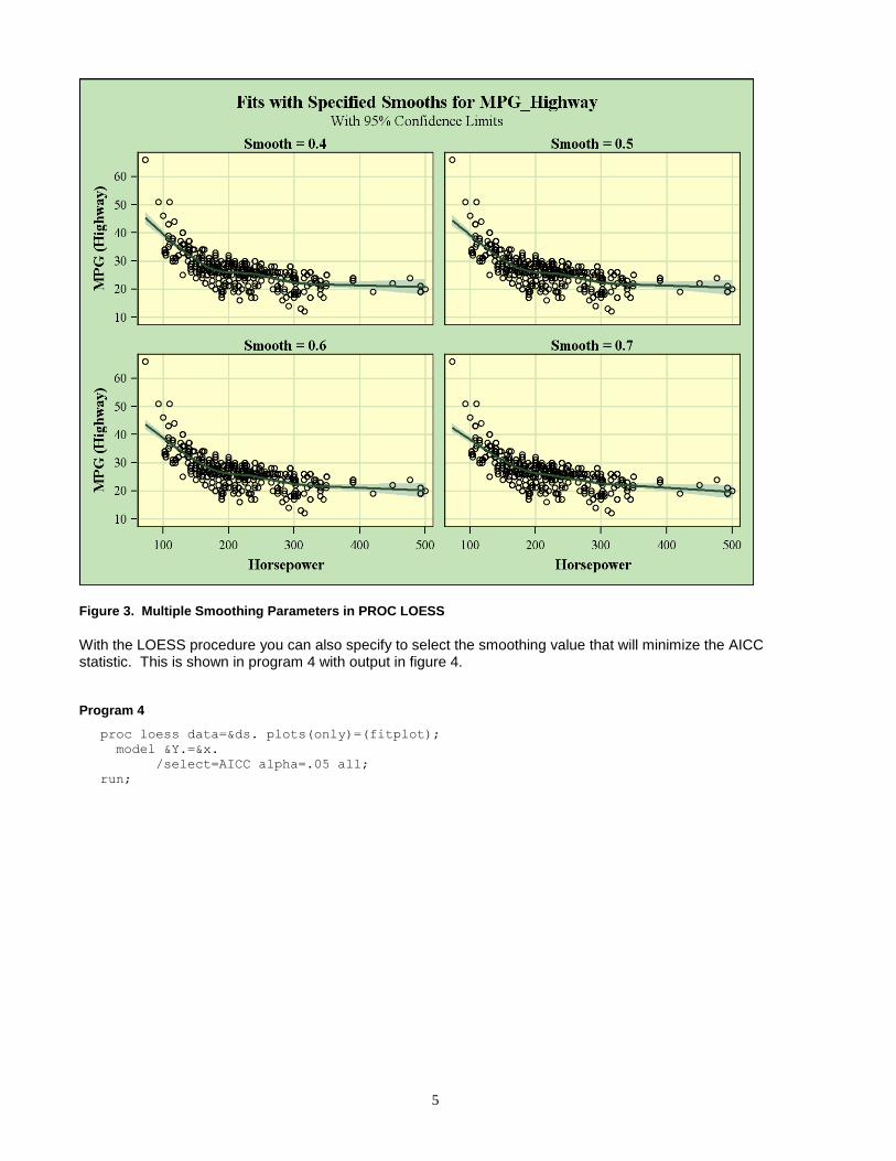
Figure 3. Multiple Smoothing Parameters in PROC LOESS

With the LOESS procedure you can also specify to select the smoothing value that will minimize the AICC statistic. This is shown in program 4 with output in figure 4.

Program 4

proc loess data=&ds. plots(only)=(fitplot);

model &Y.=&x.

/select=AICC alpha=.05 all;

run;

6

Figure 4. Using AICC Smoothing Option in PROC LOESS

You can also optimize within a range of smoothing parameters by including both a smooth option and the select=AICC option.

The LOESS procedure also provides ODS OUTPUT capability. For example, if you want to generate the plot outside of PROC LOESS you would run the following code. You can use either GPLOT or SGPLOT, whichever is more convenient. Output is displayed in figure 5.

7

Program 5

proc loess data=&ds. plots=none;

ods output outputstatistics=outstay;

model &Y.=&X.

/smooth=0.5;

run;

proc sort data=outstay;

by &x. DepVar;

run;

title2 SGPLOT of LOESS ODS Output;

proc sgplot data=outstay;

scatter y=DepVar x=&X./ markerattrs=(color=black symbol=plus size=5) ;

series y=pred x=&X./ lineattrs=(color=red thickness=5) ;

XAXIS grid;

YAXIS grid;

run;

Figure 5. Using Output from PROC LOESS in PROC SGPLOT

8

MONOTONIC SPLINES VIA PROC TRANSREG In banking and finance applications there is a goal to generate monotonic relationships. Let’s modify the sashelp.cars data to look like a consumer lending application to predict the ratio of actual credit card balances by contractual balances.

DATA CARD;

set sashelp.cars;

mob = -19.440074906367 + 0.0110486891385768*Weight;

pct_contractual = MPG_City/100 + 0.40;

run;

Let’s see how a penalized b-spline would fit the data first in figure 6:

proc sgplot data=card;

pbspline y=pct_contractual x=mob;

xaxis grid; yaxis grid;

run;

Figure 6. Penalized B-spline.

9

Graph in figure 6 looks somewhat monotonic but not perfect. Let’s try a monotonic spline with PROC TRANSREG.

%macro monotonic(nknots);

proc transreg data=CARD;

model identity(pct_contractual)=mspline(mob / nknots=&nknots.);

output out=pred predicted ;

run;

proc sort data=pred;

by MOB;

run;

proc sgplot data=pred;

scatter y=pct_contractual x=MOB/ markerattrs=(color=black symbol=plus);

series y=Ppct_contractual x=MOB/ lineattrs=GraphPrediction

legendlabel="Predicted Fit" name="series";

xaxis grid; yaxis grid;

title Monotonic Spline with &nknots. Knots.;

run;

%mend;

%monotonic(9);

Figure 7. Monotonic Spline Generated from PROC TRANSREG..

10

Output listing is shown here. Note that TRANSREG does not generate a parametric equation that describes the relationship between the 2 variables. Also note that in SAS9.22 TRANSREG does not support the option to save a model store to score other populations using PROC PLM.

TRANSREG MORALS Algorithm Iteration History for Identity(pct_contractual)

Iteration Average Maximum Criterion

Number Change Change R-Square Change Note

-------------------------------------------------------------------------

1 0.31700 4.25925 0.54459

2 0.00000 0.00000 0.69081 0.14622 Converged

RESTRICTED OR NATURAL CUBIC SPLINES Once we have identified that a relationship is not linear there are a number of possible mathematical transformations that can be done on independent variables so that generalized linear models can be used to fit the relationships. These include, but are not limited to:

Binning continuous variables into nominal binary variables (or dummy variables). These typically reduce the predictive power of the variable in a predictive model and results in a step function relationship between the predictor and the dependent variable. In addition, results often don’t validate well in out of time samples. See Irwin and McClelland (2003).

If the relationship is piecewise linear then linear splines can be used to fit the data points. However linear splines cannot fit curvilinear data.

Power and/or log transformations of the independent or dependent variable can prove useful in linearizing the relationship.

Polynomial functions and/or piecewise polynomial splines such as cubic splines can fit curved relationships.

The issue with cubic splines is that the tails of the fit often don’t behave well. As an alternative to cubic splines, restricted cubic splines force the tails to be linear and have other advantages we will review in this paper.

Fitting regression splines to data requires the introduction of knot points to the model. For linear splines, the knots indicate where a change in slope will occur. The selection of how many knots and where to place the knots are not part of the regression estimation. Knots need to be defined A Priori to the regression build based on existing theory. Often, however, prior information about functional relationships between variables is not available. An advantage of using restricted cubic splines is that placement of knots are not as important as the selection of the number of knots. Knot placement is predetermined by the cumulative percentile values of the independent variables. Table 1 shows the respective percentile cuts based on the number of knots (k) selected. Table is documented in Harrell (2010).

Table 1 Percentile Values to Determine Knot Placement with Restricted Cubic Splines

For most data sets, k=5 will produce good results. For fewer than 100 observations, k=3 will provide a good fit. One can also optimize the number of knots by minimizing AIC or AICC after trying all 5 regression runs.

Another advantage of restricted cubic splines is that the number of regression parameters are k-1 (not including the intercept). Cubic splines require k+3 terms be estimated.

k Quantiles

3 .10 .5 .90

4 .05 .35 .65 .95

5 .05 .275 .5 .725 .95

6 .05 .23 .41 .59 .77 .95

7 .025 .1833 .3417 .5 .6583 .8167 .975

11

For example, in our sample data, if we choose 5 knots, the number of terms we add to the model are 4; HORSEPOWER, HORSEPOWER1, HORSEPOWER2, HORSEPOWER3. HORSEPOWER1 – HORSEPOWER3 are cubic terms added to the model based on the cumulative distribution values for HORSEPOWER. Frank Harrell has documented a SAS RCSPLINE macro available online at

http://biostat.mc.vanderbilt.edu/wiki/pub/Main/SasMacros/survrisk.txt

For our example, program 6 will calculate the position of the knots based on the percentile cuts in table 1. Output 1 shows the result of the percentile calculation.

Program 6

proc univariate data=sashelp.cars noprint;

var horsepower;

output out=knots pctlpre=P_ pctlpts=5 27.5 50 72.5 95;

run;

proc print data=knots; run;

Obs P_5 P_27_5 P_50 P_72_5 P_95

1 115 170 210 245 340

Output 1. Percentiles Calculated from PROC UNIVARIATE

We then use a data step with the RCSPLINE macro to calculate the functional form of HORSEPOWER1 – HORSEPOWER3. This is done in program 7.

Program 7

data test;

set sashelp.cars;

%rcspline (horsepower,115, 170, 210, 245, 340);

run;

We need to take a look at the SAS log from program 7 to make note of the transformations used. The default option from the macro makes all added cubic terms in the units of the independent variable. Output 2 from the SAS LOG shows logic that calculates the additional terms (HORESPOWER1, HORSEPOWER2, HORSEPOWER3).


12

MPRINT(RCSPLINE): DROP _kd_;

MPRINT(RCSPLINE): _kd_= (340 - 115)**.666666666666 ;

MPRINT(RCSPLINE):

horsepower1=max((horsepower-115)/_kd_,0)**3+((245-115)*max((horsepower-340)/_kd_,0)**3

-(340-115)*max((horsepower-245)/_kd_,0)**3)/(340-245);

MPRINT(RCSPLINE): ;

MPRINT(RCSPLINE):



MPRINT(RCSPLINE): ;

MPRINT(RCSPLINE):



MPRINT(RCSPLINE): ;

43 run;

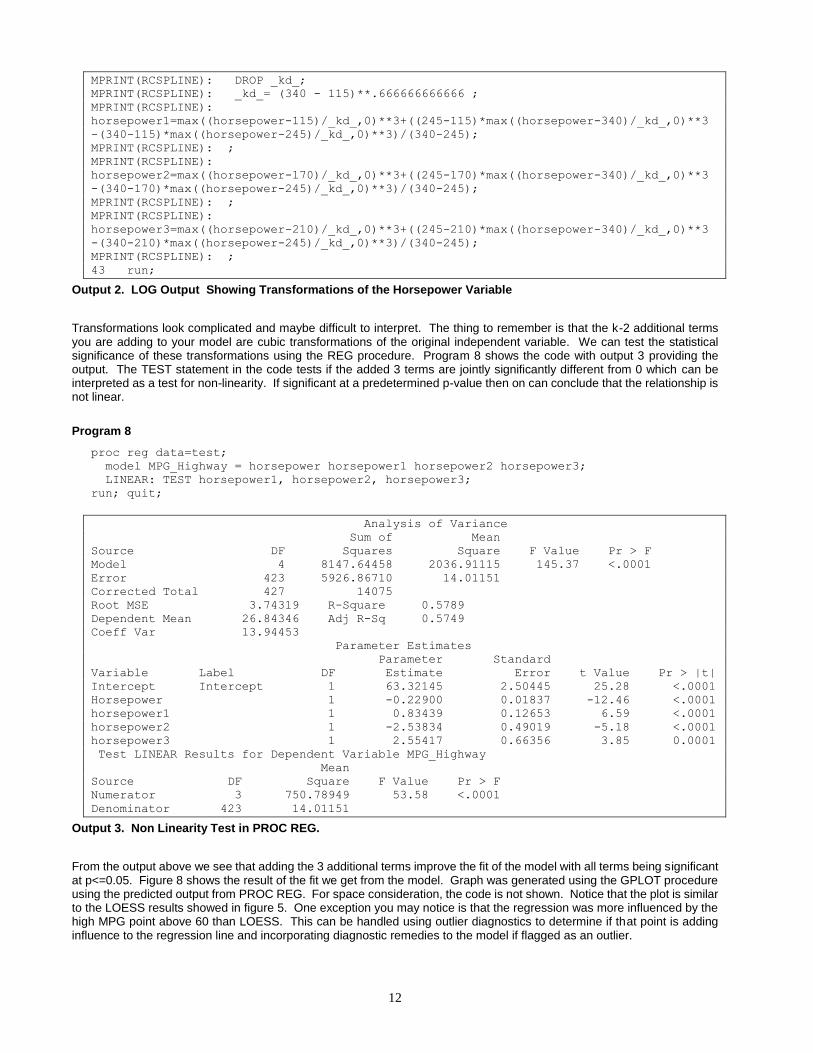
Output 2. LOG Output Showing Transformations of the Horsepower Variable

Transformations look complicated and maybe difficult to interpret. The thing to remember is that the k-2 additional terms you are adding to your model are cubic transformations of the original independent variable. We can test the statistical significance of these transformations using the REG procedure. Program 8 shows the code with output 3 providing the output. The TEST statement in the code tests if the added 3 terms are jointly significantly different from 0 which can be interpreted as a test for non-linearity. If significant at a predetermined p-value then on can conclude that the relationship is not linear.

Program 8

proc reg data=test;

model MPG_Highway = horsepower horsepower1 horsepower2 horsepower3;

LINEAR: TEST horsepower1, horsepower2, horsepower3;

run; quit;

Analysis of Variance

Sum of Mean

Source DF Squares Square F Value Pr > F

Model 4 8147.64458 2036.91115 145.37 <.0001

Error 423 5926.86710 14.01151

Corrected Total 427 14075

Root MSE 3.74319 R-Square 0.5789

Dependent Mean 26.84346 Adj R-Sq 0.5749

Coeff Var 13.94453

Parameter Estimates

Parameter Standard

Variable Label DF Estimate Error t Value Pr > |t|

Intercept Intercept 1 63.32145 2.50445 25.28 <.0001

Horsepower 1 -0.22900 0.01837 -12.46 <.0001

horsepower1 1 0.83439 0.12653 6.59 <.0001

horsepower2 1 -2.53834 0.49019 -5.18 <.0001

horsepower3 1 2.55417 0.66356 3.85 0.0001

Test LINEAR Results for Dependent Variable MPG_Highway

Mean

Source DF Square F Value Pr > F

Numerator 3 750.78949 53.58 <.0001

Denominator 423 14.01151

Output 3. Non Linearity Test in PROC REG.

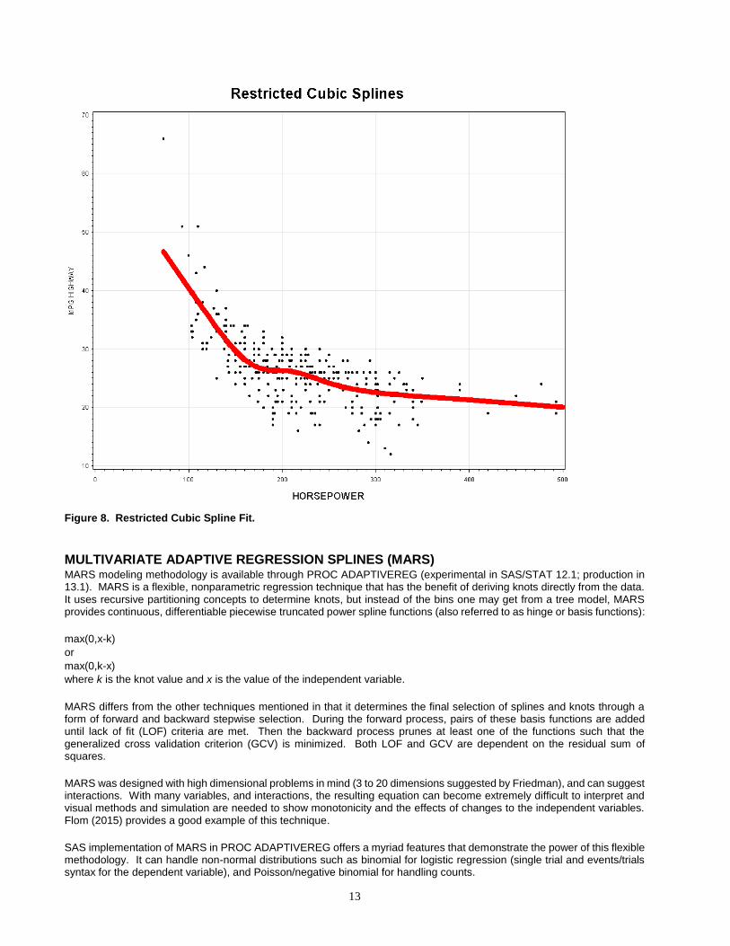
From the output above we see that adding the 3 additional terms improve the fit of the model with all terms being significant at p<=0.05. Figure 8 shows the result of the fit we get from the model. Graph was generated using the GPLOT procedure using the predicted output from PROC REG. For space consideration, the code is not shown. Notice that the plot is similar to the LOESS results showed in figure 5. One exception you may notice is that the regression was more influenced by the high MPG point above 60 than LOESS. This can be handled using outlier diagnostics to determine if that point is adding influence to the regression line and incorporating diagnostic remedies to the model if flagged as an outlier.

13

Figure 8. Restricted Cubic Spline Fit.

MULTIVARIATE ADAPTIVE REGRESSION SPLINES (MARS) MARS modeling methodology is available through PROC ADAPTIVEREG (experimental in SAS/STAT 12.1; production in 13.1). MARS is a flexible, nonparametric regression technique that has the benefit of deriving knots directly from the data. It uses recursive partitioning concepts to determine knots, but instead of the bins one may get from a tree model, MARS provides continuous, differentiable piecewise truncated power spline functions (also referred to as hinge or basis functions):

max(0,x-k)

or

max(0,k-x)

where k is the knot value and x is the value of the independent variable.

MARS differs from the other techniques mentioned in that it determines the final selection of splines and knots through a form of forward and backward stepwise selection. During the forward process, pairs of these basis functions are added until lack of fit (LOF) criteria are met. Then the backward process prunes at least one of the functions such that the generalized cross validation criterion (GCV) is minimized. Both LOF and GCV are dependent on the residual sum of squares.

MARS was designed with high dimensional problems in mind (3 to 20 dimensions suggested by Friedman), and can suggest interactions. With many variables, and interactions, the resulting equation can become extremely difficult to interpret and visual methods and simulation are needed to show monotonicity and the effects of changes to the independent variables. Flom (2015) provides a good example of this technique.

SAS implementation of MARS in PROC ADAPTIVEREG offers a myriad features that demonstrate the power of this flexible methodology. It can handle non-normal distributions such as binomial for logistic regression (single trial and events/trials syntax for the dependent variable), and Poisson/negative binomial for handling counts.

14

Let’s return to our example. The code in program 9 runs ADAPTIVEREG using default settings.

Program 9

proc adaptivereg data=sashelp.cars plots=all details=bases;

model MPG_Highway = horsepower;

run;

Output 4. PROC ADAPTIVEREG Bases and Final Model Using Defaults.

The ADAPTIVEREG Procedure

Fit Statistics

GCV 13.44050

GCV R-Square 0.59319

Effective Degrees of Freedom 15

R-Square 0.61943

Adjusted R-Square 0.61308

Mean Square Error 12.75330

Average Square Error 12.51492

Basis Information

Name Transformation

Basis0 1

Basis1 Basis0*MAX(Horsepower - 168,0)

Basis2 Basis0*MAX( 168 - Horsepower,0)



















Regression Spline Model after Backward Selection

Name Coefficient Parent Variable Knot

Basis0 1.1099 Intercept

Basis1 -0.5889 Basis0 Horsepower 168.00

Basis2 0.6016 Basis0 Horsepower 168.00






15

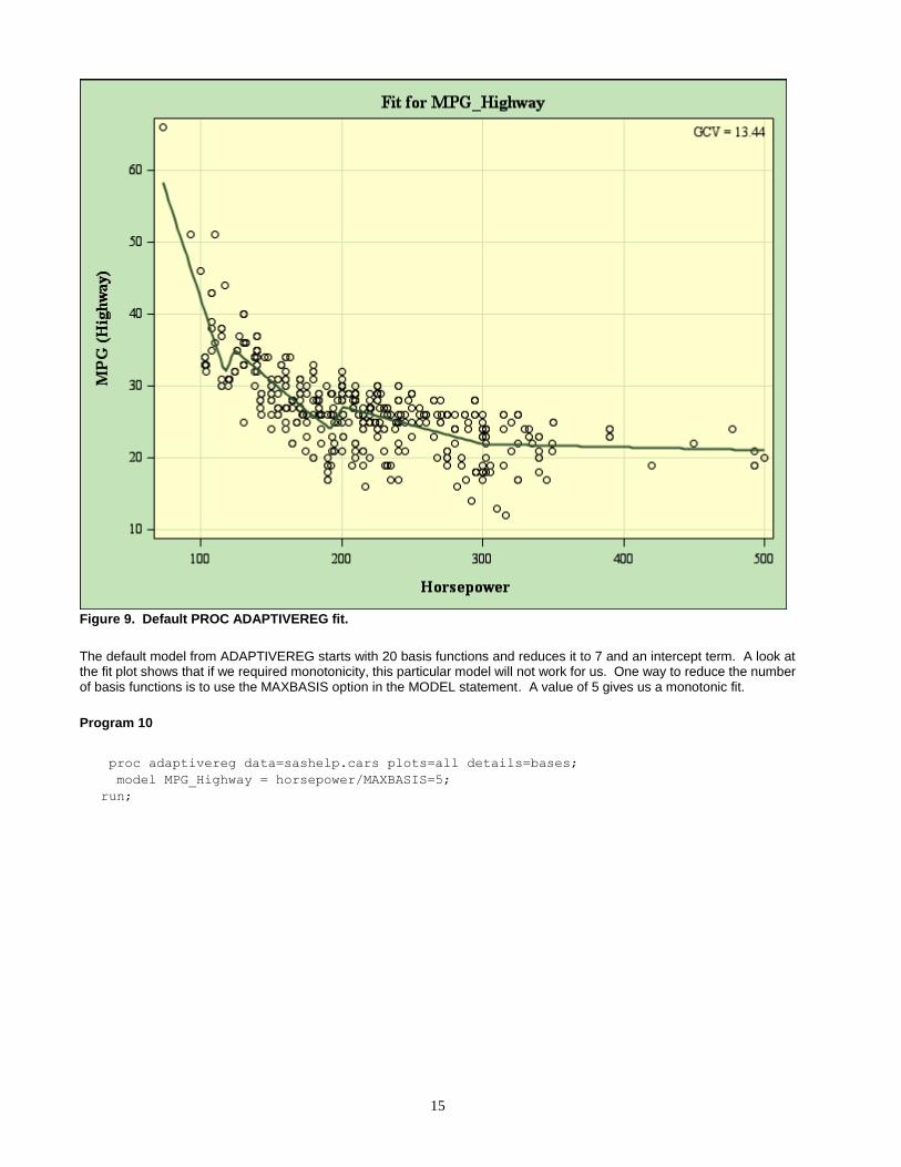
Figure 9. Default PROC ADAPTIVEREG fit.

The default model from ADAPTIVEREG starts with 20 basis functions and reduces it to 7 and an intercept term. A look at the fit plot shows that if we required monotonicity, this particular model will not work for us. One way to reduce the number of basis functions is to use the MAXBASIS option in the MODEL statement. A value of 5 gives us a monotonic fit.

Program 10

proc adaptivereg data=sashelp.cars plots=all details=bases;

model MPG_Highway = horsepower/MAXBASIS=5;

run;

16

Output 5. PROC ADAPTIVEREG Bases and Final Model with MAX.

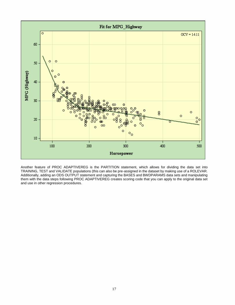
Here we get a monotonic fit with knots at 117 and 168 with 3 basis functions and an intercept.

The ADAPTIVEREG Procedure

Fit Statistics

GCV 14.11053

GCV R-Square 0.57291

Effective Degrees of Freedom 7

R-Square 0.58483

Adjusted R-Square 0.58189

Mean Square Error 13.78154

Average Square Error 13.65275

Basis Information

Name Transformation

Basis0 1





Regression Spline Model after Backward Selection

Name Coefficient Parent Variable Knot

Basis0 12.3262 Intercept




17

Another feature of PROC ADAPTIVEREG is the PARTITION statement, which allows for dividing the data set into TRAINING, TEST and VALIDATE populations (this can also be pre-assigned in the dataset by making use of a ROLEVAR. Additionally, adding an ODS OUTPUT statement and capturing the BASES and BWDPARAMS data sets and manipulating them with the data steps following PROC ADAPTIVEREG creates scoring code that you can apply to the original data set and use in other regression procedures.

18

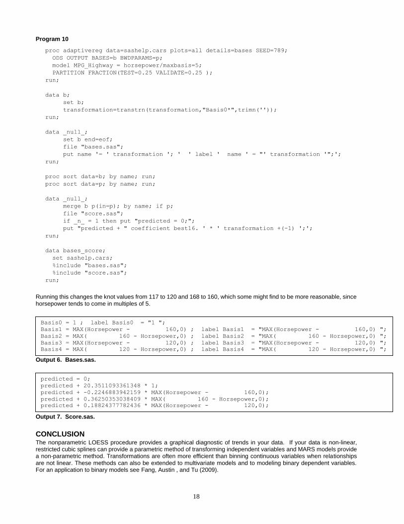
Program 10

proc adaptivereg data=sashelp.cars plots=all details=bases SEED=789;

ODS OUTPUT BASES=b BWDPARAMS=p;

model MPG_Highway = horsepower/maxbasis=5;

PARTITION FRACTION(TEST=0.25 VALIDATE=0.25 );

run;

data b;

set b;

transformation=transtrn(transformation,"Basis0*",trimn(''));

run;

data _null_;

set b end=eof;

file "bases.sas";

put name '= ' transformation '; ' ' label ' name ' = "' transformation '";';

run;

proc sort data=b; by name; run;

proc sort data=p; by name; run;

data _null_;

merge b p(in=p); by name; if p;

file "score.sas";

if _n_ = 1 then put "predicted = 0;";

put "predicted + " coefficient best16. ' * ' transformation +(-1) ';';

run;

data bases_score;

set sashelp.cars;

%include "bases.sas";

%include "score.sas";

run;

Running this changes the knot values from 117 to 120 and 168 to 160, which some might find to be more reasonable, since horsepower tends to come in multiples of 5.

Output 6. Bases.sas.

Output 7. Score.sas.

CONCLUSION

The nonparametric LOESS procedure provides a graphical diagnostic of trends in your data. If your data is non-linear, restricted cubic splines can provide a parametric method of transforming independent variables and MARS models provide a non-parametric method. Transformations are often more efficient than binning continuous variables when relationships are not linear. These methods can also be extended to multivariate models and to modeling binary dependent variables. For an application to binary models see Fang, Austin , and Tu (2009).

Basis0 = 1 ; label Basis0 = "1 ";

Basis1 = MAX(Horsepower - 160,0) ; label Basis1 = "MAX(Horsepower - 160,0) ";

Basis2 = MAX( 160 - Horsepower,0) ; label Basis2 = "MAX( 160 - Horsepower,0) ";

Basis3 = MAX(Horsepower - 120,0) ; label Basis3 = "MAX(Horsepower - 120,0) ";

Basis4 = MAX( 120 - Horsepower,0) ; label Basis4 = "MAX( 120 - Horsepower,0) ";

predicted = 0;

predicted + 20.3511093361348 * 1;

predicted + -0.2246883942159 * MAX(Horsepower - 160,0);

predicted + 0.36250353038409 * MAX( 160 - Horsepower,0);

predicted + 0.18824377782436 * MAX(Horsepower - 120,0);

19

REFERENCES:

• Akaike, H. (1973), “Information Theory and an Extension of the Maximum Likelihood Principle,” in Petrov and Csaki, eds., Proceedings of the Second International Symposium on Information Theory, 267–281.

• Cleveland, W. S., Devlin, S. J., and Grosse, E. (1988), “Regression by Local Fitting,” Journal of Econometrics, 37, 87–114.

• Cleveland, W. S. and Grosse, E. (1991), “Computational Methods for Local Regression,” Statistics and Computing, 1, 47–62.

• Fang, J., Austin ,P. C., and Tu, J. V. (2009), “Test for linearity between continuous confounder and binary outcome first, run a multivariate regression analysis second,” SAS Global Forum 2009 (paper 252-2009).

• Flom, P. (2015), “Alternative methods of regression when OLS is not right,” SAS Global Forum 2015 (paper 3412-2015).

• Friedman, J. H. (1991), “Multivariate Adaptive Regression Splines,” Annals of Statistics, 19, 1–67.

• Harrell, F. (2010). “Regression Modeling Strategies: With Applications to Linear Models, Logistic Regression, and Survival Analysis (Springer Series in Statistics),” Springer.

• Harrell, F. RCSPLINE MACRO: – http://biostat.mc.vanderbilt.edu/wiki/pub/Main/SasMacros/survrisk.txt

• Irwin, J.R. and McClelland, G.H. (2003), “Negative Consequences of Dichotomizing Continuous Predictor Variables”, Journal of Marketing Research, Vol. 40, No. 3 (Aug., 2003), pp. 366-371.

• Kuhfeld, W. F. and Cai, W. (2013), “Introducing the New ADAPTIVEREG Procedure for Adaptive Regression,” SAS Global Forum 2013 (paper 457-2013).

• Stone, C. J. and Koo, C. Y. (1985), “Additive Splines in Statistics,” In Proceedings of the Statistical Computing Section ASA, pages 45-48, Washington, DC, 1985.

• Randy Tobias and Weijie Cai (2010), “Introducing PROC PLM and Postfitting Analysis for Very General Linear Models in SAS/STAT 9.22,“ SAS Global Forum 2010.

AKNOWLEDGEMENTS Nish and Jonas would like to thank Andrea Wainwright-Zimmerman and Peter Flom for their help in making sense and good use of MARS models.

CONTACT INFORMATION Your comments and questions are valued and encouraged. Contact the author at:

Jonas V. Bilenas

Barclays Global Retail Bank

Wilmington, DE 19801

Email: [email protected]

[email protected]

Nish Herat

Verizon Wireless

Basking Ridge, NJ 07920

Email: [email protected]

[email protected]

SAS and all other SAS Institute Inc. product or service names are registered trademarks or trademarks of SAS Institute Inc. in the USA and other countries. ® indicates USA registration. Other brand and product names are trademarks of their respective companies. This work is an independent effort and does not necessarily represent the practices followed at current or previous employers.


mailto:[email protected]




paper bf-140 using regression splines in sas stat...

Documents