NOLTA, IEICE

Paper

A study on a low power optimizationalgorithm for an edge-AI device

Tatsuya Kaneko 1a), Kentaro Orimo 1, Itaru Hida 1 ,

Shinya Takamaeda-Yamazaki 1 , Masayuki Ikebe 1 ,

Masato Motomura 1, and Tetsuya Asai 1

1 Division of Electronics for Informatics, Graduate School of Information

Science and Technology (IST), Hokkaido University, M-BLDG 2F, Kita 14,

Nishi 9, Kita-ku, Sapporo, Hokkaido, 060-0814, Japan

a) kaneko.tatsuya.cy@ist.hokudai.ac.jp

Received January 8, 2019; Revised April 8, 2019; Published October 1, 2019

Abstract: Although research on the inference phase of edge artificial intelligence (AI) hasmade considerable improvement, the required training phase remains an unsolved problem.Neural network (NN) processing has two phases: inference and training. In the training phase,a NN incurs high calculation cost. The number of bits (bitwidth) in the training phase isseveral orders of magnitude larger than that in the inference phase. Training algorithms,optimized to software, are not appropriate for training hardware-oriented NNs. Therefore,we propose a new training algorithm for edge AI: backpropagation (BP) using a ternarizedgradient. This ternarized backpropagation (TBP) provides a balance between calculation costand performance. Empirical results demonstrate that in a two-class classification task, TBPworks well in practice and compares favorably with 16-bit BP (Fixed-BP).

Key Words: machine learning, edge AI, training algorithm, backpropagation, quantization,low power

1. IntroductionMany of the most successful current machine/deep learning systems rely on cloud devices such asgraphics processing unit (GPU) servers. A neural network is trained by a stochastic gradient descent(SGD) [1] method, Adam [2], and the like. These training algorithms have been used to train neuralnetworks recently. For example, Squeeze-and-Excitation networks [3] is one of the best approachesfor image recognition, CycleGAN [4] is one of the best approaches for data generation, and ParallelWaveNet [5] is one of the best at speech synthesis. These great achievements are based on high-performance and high-power-consumption devices such as GPUs. GPUs consume huge amounts ofpower, so their use on edge devices is difficult. TPUv2 [6], v3 [7], and DLU [8] are used not onlyin the inference phase but also in the training phase. In TPU, most of the computations performedin training a neural network are floating point multiplications; also in addition, DLU uses its ownprecision called “Deep Learning Integer” (DL-INT) in [8] to train a neural network. This DL-INTcan reduce power consumption while maintaining accuracy. However, these architecture are used on

373

Nonlinear Theory and Its Applications, IEICE, vol. 10, no. 4, pp. 373–389 c©IEICE 2019 DOI: 10.1587/nolta.10.373

cloud servers, so are not appropriate for edge device.On the other hand, field programmable gate arrays (FPGAs) can be used to accelerate and achieve

higher energy efficiency than GPUs. FPGAs are a user-programmable hardware; hence, we cancompose high-energy-efficiency circuits depending on each neural network. FPGAs can calculate withlow power consumption. Various types of FPGA exist from low-end to high-end. High-end FPGAsare also used in cloud servers. Our method is aimed towards the low end or requiring less resourcesthan low-end FPGAs. We call these devices edge devices. In edge devices, which have lower powerand resource requirements than GPUs, many approaches for the inference phase that can acceleratecalculation have been and are still actively being investigated. Usually, this type of accelerator usesa neural network’s parameter, which is previously trained by central processing unit (CPU) or GPU.A summary of FPGA-based accelerators was presented by Guo et al. [9] In contrast to the activearea of research investigation into the inference phase, only a few approaches for the training phase toaccelerate or even implement calculation have been investigated. This type of architecture does notuse a pre-trained parameter, it obtains its own parameter by training. For example, DoReFa-Net [10]is a method to train convolutional neural networks that have low bitwidth weights and activationsusing low bitwidth parameter gradients. This method aims at accelerating and also reducing thepower consumption of neural networks by quantization or binarization. F-CNN [11] also aims ataccelerating and reducing the power consumption of neural networks by reconfiguring a streamingdatapath at runtime. However, F-CNN uses 32-bit floating-point arithmetic, so we do not considerthis method as appropriate for edge devices.

The reason for the lack of investigations into training for edge devices is that training is more difficultthan inference. Neural networks in the training phase deal with minimum values: networks need agreater number of bits for the data representation. As the bitwidth increases, so do the resourcesrequired. To tackle the issue of the bitwidth, to allow networks to train and guarantee reasonableaccuracy with edge devices, all previous methods used an unbalanced approach between resources andperformance. Our method can provide a balance between resources and performance. In the not toodistant future, we consider that training algorithms for edge devices will gain in importance: relyingon today’s cloud servers for training every neural network is difficult. There has been growing interestin machine/deep learning, so that we need to use simple devices according to task and not use cloudservers for every task.

This paper makes the following contributions.

1. We propose a backpropagation architecture and low-power and low-resource algorithm. Thearchitecture is based on the SGD method; it uses fixed-point multiplications to calculate theforward pass and backward pass. A bitwidth in this architecture is defined by experiment.Our proposed algorithm is aimed at edge devices: it uses ternarized gradient to calculate thebackward pass.

2. We introduce our proposed algorithm: “ternarized backpropagation” (TBP). TBP has twoimportant components, mutation, rate of changing parameters, and L2 regularization. Weexplore the configuration space of mutation for TBP. For example, training a network using a0.3% mutation rate can lead to the highest accuracy on the MNIST dataset. In addition, we showthat a lower mutation rate is better than a higher mutation through experiment. Furthermore,we show the importance of L2 regularization to prevent accuracy from being reduced.

3. We show that the TBP algorithm consumes less power than 16-bit quantized backpropagationby two orders magnitude on the same task, which is two-class classification task using an in-dependent dataset. In this experiment, we use a multilayer perceptron (MLP) on the MNISTdataset and fashion MNIST dataset; we estimate power consumption from the number of reador write operations to static random access memory (SRAM).

374

2. Proposed architecture

In this section, we introduce two types of architecture: a quantized SGD architecture implementedon FPGA and a ternarized SGD that is not implemented on any hardware, just an algorithm. Bothtypes of architecture are calculated by time division.

2.1 Fixed-BP architectureMany of the most successful artificial intelligent systems, such as machine translation, image recog-nition, and data generation, are software oriented. In these systems, the optimization algorithm usedto train a neural network is based on floating point calculation. In hardware implementations, float-ing point calculation needs more power and resources than fixed-point calculation; we do not usefloating point under the constraint condition that edge devices require low power consumption andresources. We consider that quantizing to SGD is the simplest method to train neural networks onedge device. One of the most important problems when using fixed-point calculation is the relationbetween bitwidth and accuracy. We have confirmed how the bitwidth can achieve better accuracy bysoftware simulation using MLP on the MNIST dataset [12]. Figure 1 shows the network model: thenumber of neurons is 784–150–10 (this parameter is limited by the memory size of the target hard-ware device), the bitwidth in the inference phase is 8 bits, 1–2–5 bit (sign–integer–fractional part),the activation function of each layer is a sigmoid function, the learning rate is 0.4, the minibatch sizeis 1, and the training iteration is 0.3 epochs (18,000 iterations). Figure 2 shows the relation betweenthe bitwidth and accuracy; a power-of-two bitwidth is favorable for SRAM, so that we have simulatedhow accuracy changes about each power-of-two bitwidth. On the basis of this result, we found thatthe neural network needs more 16-bit bitwidths in the training phase to achieve better accuracy withMNIST test. We thus use 16 bits as the bitwidth in the training phase. We cannot implement onlybackpropagation, so that the inference phase has also been implemented in this architecture.

In the real world, the environment is changing so slowly as compared to present digital computers,and hence we consider edge devices do not require high throughput. In other words, edge devices

Fig. 1. Network model. We use MLP, which has one hidden layer. Thebitwidth in the inference phase is 8 bits and in training phase is 32, 16, or 8bits.

Fig. 2. Average of 30 times accuracy at each bitwidth in the training phase.

375

are not appropriate accelerators; that is, they do not have high-performance processors or high-speedinterfaces. Even if we achieve high-speed calculation using parallel operation, throughput is limitedby the low-speed interface (SPI, I2C [13]), so that using parallel operation to achieve high throughputis not important. We thus decided to use serial operation in forward and backward propagation.

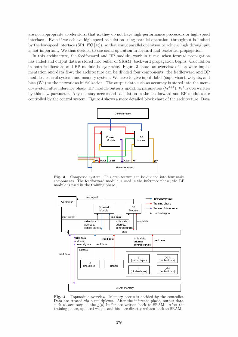
In this architecture, the feedforward and BP modules work in turns: when forward propagationhas ended and output data is stored into buffer or SRAM, backward propagation begins. Calculationin both feedforward and BP module is layer-wise. Figure 3 shows an overview of hardware imple-mentation and data flow; the architecture can be divided four components: the feedforward and BPmodules, control system, and memory system. We have to give input, label (supervisor), weights, andbias (W0) to the network as initialization. The output data such as accuracy is stored into the mem-ory system after inference phase. BP module outputs updating parameters (Wt+1); Wt is overwrittenby this new parameter. Any memory access and calculation in the feedforward and BP modules arecontrolled by the control system. Figure 4 shows a more detailed block chart of the architecture. Data

Fig. 3. Composed system. This architecture can be divided into four maincomponents. The feedforward module is used in the inference phase; the BPmodule is used in the training phase.

Fig. 4. Topmodule overview. Memory access is decided by the controller.Data are treated via a multiplexer. After the inference phase, output data,such as accuracy, in the g(y) buffer are written back to SRAM. After thetraining phase, updated weight and bias are directly written back to SRAM.

376

is temporarily stored into input buffers (x, t) to reduce SRAM access; however, weights and biasesare stored into SRAM owing to the huge number of values. We stored each layer’s output data intog(h) and g(y) in output buffers. The outputs of the hidden and output layers are stored in buffersg(h) and g(y), respectively. In the training phase, these outputs are used to calculate error gradientor to update parameters so that both values must be stored until the training phase is completed. Ifthis architecture has an inference phase only, two buffers are not required. in addition, we have tostore each layer’s “raw” output, before putting in activations, into output buffers (h, y); raw outputis also used in the training phase. The controller module generates signals such as memory address;SRAM or buffer access is controlled by these signals via a multiplexer (MUX). More details of thefeedforward and BP modules are given in the following.

Feedforward and BP modules use time-divided calculation to reduce hardware resources. In onecalculation cycle, one weight is read from SRAM. Activation functions and their differentials areimplemented by a look-up table (LUT). Figure 5 shows the details of the feedforward module. Thismodule is composed of three states: wait, hidden calculation, and output calculation. We haveimplemented inner production by the multiplication module (mul) and accumulation via the additionmodule (add). The input for the multiplication module is weight or bias, which is stored into SRAM,and input data, which is stored into buffer x or buffer g(h). If the input data are for the hiddenlayer, they are stored in buffer x. If instead the input data are for the output layer, they are storedin buffer g(h). When the calculation for one neuron is completed, the output value is stored in bufferh or y; in addition, buffer g(h) or g(y) stores the output value via LUT. After output calculation,the feedforward module enters wait mode until the end of the BP module calculation. Figure 6shows the detail of the BP module. This module is also composed of three states denoted “wait”,“updating output layer”, and “updating hidden layer”. When calculating the error gradient (δm),we can derive subtraction form from the differential of the loss function in many cases of machinelearning. The error gradient calculation needs a supervisor (t) and raw output of the network (y).When this calculation has ended, we can calculate the updating parameter (w′

m) and error gradientfor the previous layer (δm−1). This updating calculation needs error gradient (δm), parameters (wm),and input (hm or xm is stored into buffers) of the target layer; the learning rate is implemented by bitshift. The inner product of the error-gradient calculation is implemented by the multiplication (mul)and accumulation (accumulator) modules. The updating parameter and error gradient propagationare calculated in parallel. We do not have to propagate the error gradient until the input layer; if wehave propagated error gradient until the input layer, there are no parameters.

Fig. 5. Feedforward module. The calculation result is independently storedinto buffers: one is directly stored into each layer’s buffer, another is storedinto each layer’s activation buffers after putting into the LUT.

377

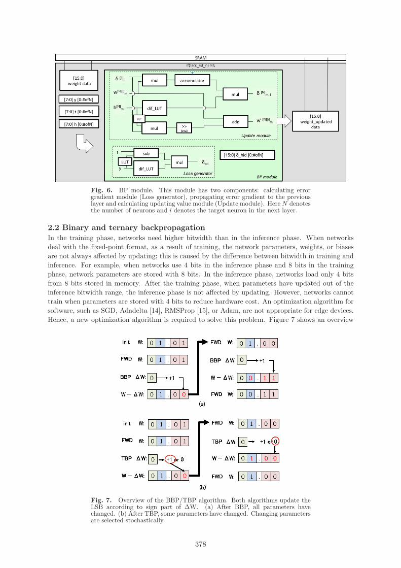
Fig. 6. BP module. This module has two components: calculating errorgradient module (Loss generator), propagating error gradient to the previouslayer and calculating updating value module (Update module). Here N denotesthe number of neurons and i denotes the target neuron in the next layer.

2.2 Binary and ternary backpropagation

In the training phase, networks need higher bitwidth than in the inference phase. When networksdeal with the fixed-point format, as a result of training, the network parameters, weights, or biasesare not always affected by updating; this is caused by the difference between bitwidth in training andinference. For example, when networks use 4 bits in the inference phase and 8 bits in the trainingphase, network parameters are stored with 8 bits. In the inference phase, networks load only 4 bitsfrom 8 bits stored in memory. After the training phase, when parameters have updated out of theinference bitwidth range, the inference phase is not affected by updating. However, networks cannottrain when parameters are stored with 4 bits to reduce hardware cost. An optimization algorithm forsoftware, such as SGD, Adadelta [14], RMSProp [15], or Adam, are not appropriate for edge devices.Hence, a new optimization algorithm is required to solve this problem. Figure 7 shows an overview

Fig. 7. Overview of the BBP/TBP algorithm. Both algorithms update theLSB according to sign part of ΔW. (a) After BBP, all parameters havechanged. (b) After TBP, some parameters have changed. Changing parametersare selected stochastically.

378

of our proposed algorithms, which are binarized backpropagation (BBP) and TBP. Both algorithmsupdate the least significant bit (LSB) according to sign bit of update value (ΔW). In BBP and TBP,gradients have been calculated with binary or ternary values; hence, we reduce the calculation cost inthe training phase by using an XNOR gate or multiplexer instead of multiplier. Furthermore, we canskip derivative calculation of the activation functions according to the gradient of activation functions.

Table I shows the accuracy of MNIST classification: the network is MLP with 784 input neurons,128 hidden neurons, 10 output neurons, and each layer has bias, and has been trained on 1 epochwith minibatch size 64. Leaky ReLU [16] and a sigmoid function are used for activations. BBP hasa high learning rate owing to updating all parameters, because the accuracy is low. On the basis ofthese results, we need to reduce the learning rate. TBP uses a ternarized gradient, +1, −1, and 0,thus we can reduce the apparent learning rate by updating a parameter with a 0 value.

Table I. MLP trained on the MNIST dataset. The accuracy is 1 epoch after.

BBP [%] TBP [%]#1 8.57 76.2#2 2.59 77.0#3 7.00 76.6#4 8.21 76.0#5 7.19 78.0

MutationWe now define mutation. Mutation is a hyper-parameter related to updating parameters. If mutationis 0%, the accuracy is the same score as initializing networks, because parameters are not updated.Similarly, if mutation is 100%, the accuracy has the same score as BBP. ΔW seldom equals 0, andtherefore TBP and BBP are equivalent if the mutation rate is 100%. Strictly speaking, TBP andBBP are only approximately equivalent. In general, from the perspective of accuracy and powerconsumption, a low mutation rate is better. Figure 8 shows that when mutation is 0.3%, the networkobtained the highest accuracy. We find that the higher the mutation rate, the lower the accuracy.Furthermore, when the network has low mutation, as a result of reducing memory access for read orwrite operations, this reduces power consumption.

Fig. 8. Dependence of accuracy on the mutation rate. Having completedfive runs, the black line represents the mean value, the red line represents thehighest score out of the five runs, and the blue line the lowest score. A mutationrate of 0.3% yields the highest accuracy.

Figure 9 shows the result of changing parameters on Fixed-BP. We can treat that this changingis similar to mutation; mutation in Fixed-BP do not change at a constant rate. We consider thatit becomes a parameter of layer and iteration. In contrast, mutation in TBP is not parameterizedby layer and iteration. In addition, the mutation rate of TBP is so low that the network may be

379

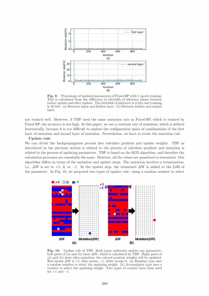
Fig. 9. Percentage of updated parameters of Fixed-BP with 1 epoch training.This is calculated from the difference in bitwidth of inference phase betweenbefore update and after update. The bitwidth of inference is 8 bits and trainingis 16 bits. (a) Between input and hidden layer. (b) Between hidden and outputlayer.

not trained well. However, if TBP used the same mutation rate as Fixed-BP, which is trained byFixed-BP, the accuracy is not high. In this paper, we use a constant rate of mutation, which is definedheuristically, because it is too difficult to explore the configuration space of combinations of the firstlayer of mutation and second layer of mutation. Nevertheless, we have to revise the mutation rule.

Update ruleWe can divide the backpropagation process into calculate gradient and update weights. TBP asintroduced in the previous section is related to the process of calculate gradient and mutation isrelated to the process of updating parameters. TBP is based on the SGD algorithm, and therefore thecalculation processes are essentially the same. However, all the values are quantized or ternarized. Ouralgorithm differs in terms of the mutation and update steps. The mutation involves a ternarization,i.e., ΔW is set to +1, 0, or −1. In the update step, the ternarized ΔW is added to the LSB ofthe parameter. In Fig. 10, we proposed two types of update rule: using a random number to select

Fig. 10. Update rule of TBP. Both types uniformly update any parameter.Left parts of (a) and (b) show ΔW, which is calculated by TBP. Right parts of(a) and (b) show after mutation; the colored position weights will be updated.Red means ΔW is +1, blue means −1, white means 0. (a) Random type usesa random number to select the updating weight. (b) Accumulator type uses acounter to select the updating weight. Two types of counter have been usedfor +1 and −1.

380

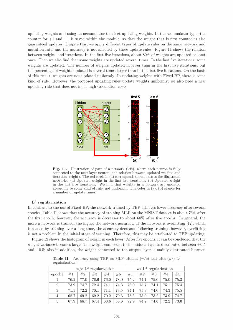
updating weights and using an accumulator to select updating weights. In the accumulator type, thecounter for +1 and −1 is saved within the module, so that the weight that is first counted is alsoguaranteed updates. Despite this, we apply different types of update rules on the same network andmutation rate, and the accuracy is not affected by these update rules. Figure 11 shows the relationbetween weights and iterations. In the first five iterations, about 80% of weights are updated at leastonce. Then we also find that some weights are updated several times. In the last five iterations, someweights are updated. The number of weights updated in fewer than in the first five iterations, butthe percentage of weights updated is several times larger than in the first five iterations. On the basisof this result, weights are not updated uniformly. In updating weights with Fixed-BP, there is somekind of rule. However, the proposed updating rules update weights uniformly; we also need a newupdating rule that does not incur high calculation costs.

Fig. 11. Illustration of part of a network (left), where each neuron is fullyconnected to the next layer neuron, and relation between updated weights anditerations (right). The red circle in (a) corresponds to red lines in the illustratednetworks. (a) Updated weight in the first five iterations. (b) Updated weightin the last five iterations. We find that weights in a network are updatedaccording to some kind of rule, not uniformly. The color in (a), (b) stands fora number of update times.

L2 regularizationIn contrast to the use of Fixed-BP, the network trained by TBP achieves lower accuracy after severalepochs. Table II shows that the accuracy of training MLP on the MNIST dataset is about 76% afterthe first epoch; however, the accuracy is decreases to about 68% after five epochs. In general, themore a network is trained, the higher the network accuracy. If the network is overfitting [17], whichis caused by training over a long time, the accuracy decreases following training; however, overfittingis not a problem in the initial stage of training. Therefore, this may be attributed to TBP updating.

Figure 12 shows the histogram of weight in each layer. After five epochs, it can be concluded that theweight variance becomes large. The weight connected to the hidden layer is distributed between +0.5and −0.5; also in addition, the weight connected to the output layer is mainly distributed between

Table II. Accuracy using TBP on MLP without (w/o) and with (w/) L2

regularization.

w/o L2 regularization w/ L2 regularizationepoch↓ #1 #2 #3 #4 #5 #1 #2 #3 #4 #5

1 76.2 77.0 76.6 76.0 78.0 75.2 74.1 75.0 75.0 75.32 73.9 74.7 72.4 74.1 74.3 76.0 75.7 74.1 75.1 75.43 71.5 72.2 70.1 71.1 73.5 74.1 75.3 74.0 74.3 75.54 68.7 69.2 69.2 70.2 70.3 73.5 75.0 73.2 73.9 74.75 67.9 66.7 67.4 68.6 68.6 72.9 74.7 74.6 72.2 73.0

381

Fig. 12. Histogram of weight without L2 regularization. (a) Weights betweeninput and hidden layers. (b) Weights between hidden and output layers.

+1.0 and −1.0. The reason for the decrease in accuracy is that the weight variance is increased.Hence, we have introduced L2 regularization to prevent the increase in weight variance. The resultsof L2 regularization are shown in Fig. 13. As a result of L2 regularization, the accuracy is about 75%after the first epoch and about 73% after five epochs. L2 regularization helps to stem the decrease inaccuracy and the increase in variance, but it does so imperfectly.

Fig. 13. Histogram of weight with L2 regularization. (a) Weights betweeninput and hidden layers. (b) Weights between hidden and output layers.

Based on this result, TBP using all ternarized gradients is incapable of the achieving a high-accuracyperformance; therefore, we do not ternarized all gradients, only the error gradient is not ternarized.Table III shows the accuracy, which is used multi bit for error gradient. We confirmed that accuracyis improved using over 4 bit for error gradient. The hardware resources and performance have beenbalanced, because the new TBP stored the relation of the error gradient among neurons instead ofthe error gradient. In practice, we define the error gradient as quantized after bit shift to the rightby one bit; this leads to achieving reasonable accuracy from the perspective of the balance betweenperformance and resource requirements.

Table III. The accuracy using multi bit for error gradient.

3bit 4bit 5bit 6bitepoch: 1 77.01% 82.46% 82.84% 84.23%epoch: 2 78.49% 81.73% 83.14% 83.29%epoch: 3 77.91% 81.97% 82.71% 83.71%epoch: 4 78.16% 81.78% 81.56% 82.00%epoch: 5 76.88% 83.07% 82.08% 80.57%

382

AlgorithmAlgorithm 1 lists the pseudo-code of our proposed algorithm TBP. Our method is based on SGD.Here L is the number of layers of weight. For example, in the case L = 2, MLP is composed of input,hidden, and output layers. With δl

q = quantize(δl � 1) we denote the error gradient, which has onlybeen quantized in TBP. The value 1 in this equation is a hyper-parameter. The larger this hyper-parameter is, the larger the bitwidth required in the error gradient. When l = 1, the error gradientis not propagated to previous layer. As a result of storing only the error gradient with quantized, wecan skip multiplication in inner product. With Mutation(Δθt) � n − λ × Mutation(θl

t), mutationbetween Δθt and θl

t is not independent, therefore L2 regularization is only applied to updating θt.As a result of mutation, if some Δθt is changed to 0, L2 regularization is not applied. Here λ is ahyper-parameter, and we define this hyper-parameter as 0.5 following experiments on the MNISTdataset.

Algorithm 1 Ternarized Back Propagation (TBP). Here E is the loss function, y is the output ofeach layer, ternarize(X) denotes ternarize, mutation(X) denotes mutation methods, L is the numberof layers of weight, θ is a parameter, and λ is a parameter of L2 regularization.Require: Network parameters W, b ∈ θ

Require: Input data x at each layerRequire: bitwidth n of fractional part in inference phase.

δL = ∂E∂yL

for l = L to 1 doδlq = quantize(δl � 1)

if l �= 1 thenδl−1 = ternarize(W l) · δl

q

end ifΔθ = ternarize(x) · δl

q

Δθt = ternarize(Δθ)θl

t+1 = θlt − Mutation(Δθt) � n − λ × Mutation(θl

t)end for

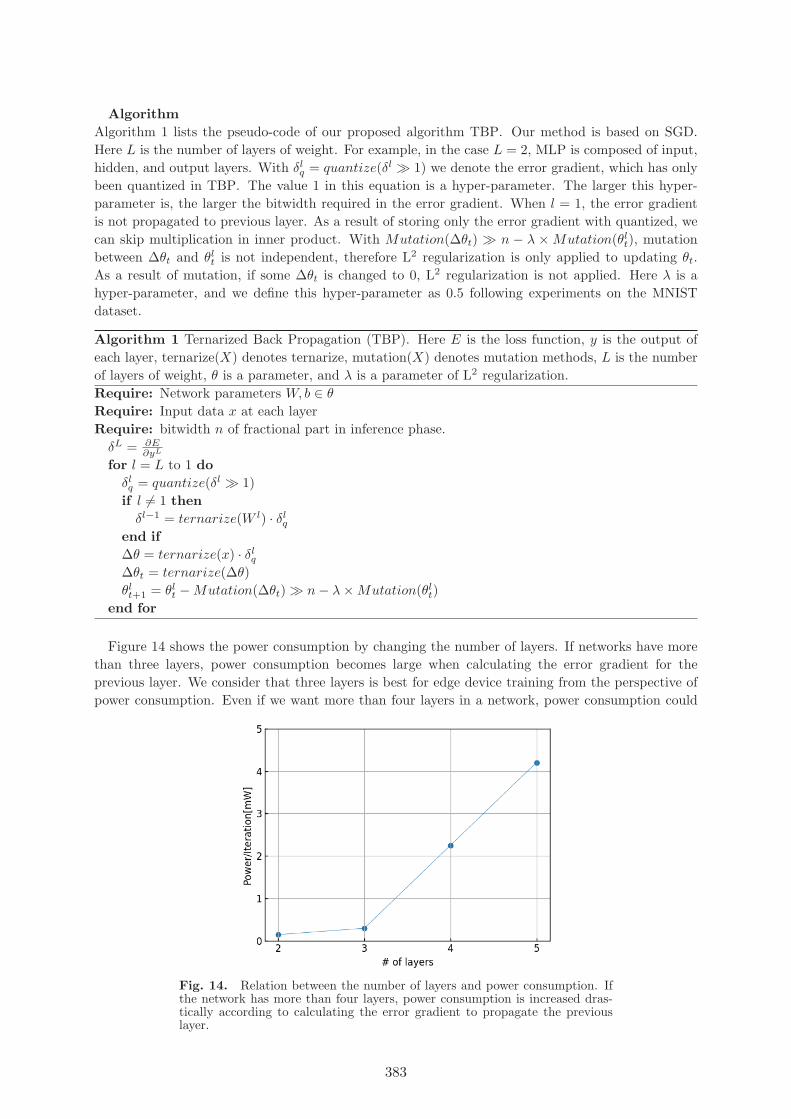
Figure 14 shows the power consumption by changing the number of layers. If networks have morethan three layers, power consumption becomes large when calculating the error gradient for theprevious layer. We consider that three layers is best for edge device training from the perspective ofpower consumption. Even if we want more than four layers in a network, power consumption could

Fig. 14. Relation between the number of layers and power consumption. Ifthe network has more than four layers, power consumption is increased dras-tically according to calculating the error gradient to propagate the previouslayer.

383

be reduced by selecting the weight to update.Architecture

Figure 15 shows the architecture of a random-type TBP module. It consists of an inner productmodule (dot), ternarize module (sign/0), and selector. Here δl and x are put in inner product moduleto calculate ΔW. The ΔW is stochastically ternarized by a random number to the handed updatemodule. TBP can skip calculating the derivative activation in the case that the activation has auniform gradient such as a sigmoid. On the other hand, δl and W are also put into the innerproduct module to calculate the previous layer’s δl−1; this operation does not require as much time ascalculating ΔW. Hence, we can this process time-multiplexed. Figure 16 shows the architecture of anaccumulator-type TBP module. It also consists of an inner product module (dot), ternarize module(sign/0), and selector. The accumulator-type TBP module has a selector more than the random type.This is attributed to the two types of counter: +1 (cnt+) and −1 (cnt-). In the accumulator-type TBPmodule, the process of inner product and ternarize is the same as in the random-type TBP module.The first bit “[0]” after the ternarized module means +1 or −1, the second bit “[1]” means whether0. That is, +1 means 00 after the ternarized module. If the count is over threshold in each countermodule, the counter module puts out +1 or −1 via the selector. Figure 17 shows the architectureof an update module. The number of times to read parameters from SRAM memory (MEM W) isnot affected by the implementation of L2 regularization: we can implement L2 regularization withoutadditional power consumption. A value of 4 in “�4” means the bitwidth of the fractional part inthe reference phase; the value of 2 in “�2” means rate of L2 regularization. Less than 1% of theentire parameters have been updated; hence, we reduce the power consumption using a write-backoperation. Figure 18 shows an overview of the backpropagation architecture; the weights have beenstored by dividing the sign part (W sign MEM) and value part (W value MEM) and using only thesign part of the parameters so that we can reduce calculation cost. The error gradient is stored intoδ-MEM, the hidden layer’s output is stored in Y -MEM. The address of this memory is operated bythe controller module for the inner product and updating parameters.

Fig. 15. Illustration of a random-type architecture.

Fig. 16. Illustration of an accumulator-type architecture.

Fig. 17. Illustration of an update module architecture.

384

Fig. 18. Overview of the backpropagation architecture.

3. Experiments

Figure 19 summarizes our approach. The proposed BBP algorithm cannot achieve our goal, andtherefore we optimized the mutation rate to use TBP. We then confirmed that the accuracy decreaseswith every iteration, and therefore we implemented L2 regularization. Next, we seek to improve theaccuracy by considering the error gradient as a series of bits. Based on these results, we performedmore practical simulations in section 3. Section 3.1 considered a 10-class classification using theMNIST dataset; i.e., the network was trained using 60,000 training data. We then measured theaccuracy using 10,000 test data. This experiment involved 30 epochs and 64 minibatches, givingapproximately 900 iterations per epoch. There were 10 output neurons. Section 3.2, on the otherhand, considered 2-class classification using both the MNIST and the fashion-MNIST datasets; i.e.,the network aimed to distinguish between input data from both datasets. This experiment exploredhow the data size and the number of iterations can be used to achieve an accuracy better than 99%.The minibatch size is 1, giving 1 iteration per epoch. There is therefore 1 output neuron as a resultof the 2-class classification. We evaluate both Fixed-BP and TBP with a software simulation usingNumpy from the perspective of accuracy and power consumption. The network is composed of three-layer MLP, input, 128 hidden units, and output layer. The network using activation function as aLeaky ReLU (leak=0.25) and a sigmoid function; also in addition, the loss function is a mean squarederror (MSE). The hyper-parameters used in the experiments are as follows. In Fixed-BP, the learningrate is 0.25. The bitwidth in the inference phase is 1 bit for the sign part, 2 bits for the integer part,and 5 bits for the fractional part, and in the training phase is 1 bit for the sign part, 2 bits for the

Fig. 19. Simulation flowchart.

385

integer part, and 13 bits for the fractional part. In TBP, mutation is 0.003 (= 0.3%). The updaterule is random type and regularization rate (λ) is 0.5. The bitwidth in the inference phase is 2 bitsfor the sign part, 2 bits for the integer part, and 4 bits for the fractional part, and in the trainingphase is 2 bits for the sign part and 3 bits for the fractional part.

3.1 MNISTIn the MNIST test, we found that TBP cannot provide a balance between high accuracy and lowpower consumption. Figure 20 shows the accuracy and power consumption on MNIST classification.We compare TBP with Fixed-BP using a minibatch size of 64. In contrast to the accuracy of Fixed-BP, TBP makes slow progress in increasing the accuracy in the entire stage of training; in addition, wefound the highest accuracy is lower than with Fixed-BP. This may be attributed to the randomnessof the update rule: as introduced in the previous section, the weight should be updated according tosome kind of rule. However, all weights are treated equally by both update rules in TBP, so that TBPmight causing the weights that should be updated to not be updated and, conversely, the weights thatshould not be updated being updated. Hence, TBP roughly increases the accuracy and sometimesdecreases the accuracy, as in the 15th epoch. We consider that a new update rule is required thatdoes not depend on randomness to solve this problem; also in addition, we possibly need a mutationschedule as in simulated annealing [18].

Fig. 20. Relation between the epoch and accuracy/power consumption. Theline shows the accuracy. The red line is the mean of 50 runs. The dotted lineshows the power consumption calculated by iteration.

The aim of this paper is only to propose a new training algorithm and not to implement it onhardware devices, such as FPGAs. Ideally, any discussion of power consumption must refer to anactual implementation on a FPGA, which is outside the scope of the present work. It is nonethelessnecessary to discuss power consumption. Our new algorithm targets edge devices, which require lowpower. The power consumed in the logical part of a FPGA (part of the Xilinx Virtex II family, whichuses 0.15 μm technology) is of the order of 10−6 W/MHz [19]. On the other hand, a read or writeoperation in SRAM [20], which uses 0.18 μm technology, 2 ports and O(103Bytes), consumes theorder of 10−3 W/MHz. From these results, we conclude that SRAM access dominates over arithmeticoperations. So that, the power consumption is estimated by the number of read and write operationsto SRAM [20]. On the basis of accuracy and power consumption, Fixed-BP is more suitable thanTBP; however, in edge devices, we consider that it is too difficult to apply to the training algorithm,which needs O(103) power consumption. If we do not need as high accuracy, such as over 90% todiscriminate, we can consider using TBP to reduce power consumption. TBP has a weak point as

386

increasing the accuracy is a slow process; conversely, TBP does not require a long training timelike Fixed-BP. We can achieve reasonable power consumption and accuracy using TBP with >3epochs. Thus, TBP cannot achieve both high accuracy and low power consumption at the same time;however, if we do not require high accuracy, TBP can provide a balance between hardware cost andperformance.

3.2 FilteringWe consider that edge devices are more appropriate for two-class classification, such as filtering, thanMNIST classification. In the approaching “Internet of Things” (IoT) era, one of the most importanttasks will be that of selecting whether data is necessary to use network bandwidth. We consider thatdata should be distinguished if it has an independent distribution. Therefore, we evaluate both Fixed-BP and TBP on classification using two types of dataset, digit or fashion: T-shirt, dress, sandal, bag,etc. In this test, a number of output neurons have been changed to 1.

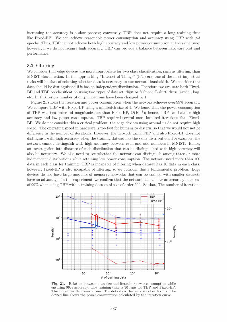
Figure 21 shows the iteration and power consumption when the network achieves over 99% accuracy.We compare TBP with Fixed-BP using a minibatch size of 1. We found that the power consumptionof TBP was two orders of magnitude less than Fixed-BP, O(10−1); hence, TBP can balance highaccuracy and low power consumption. TBP required several more hundred iterations than Fixed-BP. We do not consider this a critical problem: the edge devices using around us do not require highspeed. The operating speed in hardware is too fast for humans to discern, so that we would not noticedifference in the number of iterations. However, the network using TBP and also Fixed-BP does notdistinguish with high accuracy when the training dataset has the same distribution. For example, thenetwork cannot distinguish with high accuracy between even and odd numbers in MNIST. Hence,an investigation into distance of each distribution that can be distinguished with high accuracy willalso be necessary. We also need to see whether the network can distinguish among three or moreindependent distributions while retaining low power consumption. The network need more than 100data in each class for training. TBP is incapable of filtering when dataset has 10 data in each class;however, Fixed-BP is also incapable of filtering, so we consider this a fundamental problem. Edgedevices do not have large amounts of memory; networks that can be trained with smaller datasetshave an advantage. In this experiment, we confirm that the network can achieve an accuracy in excessof 99% when using TBP with a training dataset of size of order 500. So that, The number of iterations

Fig. 21. Relation between data size and iteration/power consumption whileensuring 99% accuracy. The training time is 30 runs for TBP and Fixed-BP.The line shows the mean of runs. The dots show the real data of each runs. Thedotted line shows the power consumption calculated by the iteration curve.

387

does not decrease, even for datasets greater than 2,000. Thus, TBP can achieve both high accuracyand low power consumption at the same time in filtering tests using an independent data distribution.On the other hand, TBP and also Fixed-BP cannot achieve high accuracy in filtering tests using thesame distribution, such as distinguishing between even and odd numbers in the MNIST dataset.

4. ConclusionWe introduced a simple and computationally efficient algorithm for gradient-based optimization. TheTBP is aimed at machine-learning problems with edge devices, which require low power consumption.The experiments confirmed the advantage of TBP in filtering tasks: we demonstrated that the powerconsumption of the proposed TBP was lower than that of the 16-bit BP (Fixed-BP) by two ordersof magnitude in a two-class classification task while ensuring 99% accuracy. In contrast to cloudartificial intelligence (AI) processing, which is used to achieve high accuracy in complex tasks, edge-AI processing is used for simple classification tasks; in these tasks, edge AI will be required to workin various environments. In any environment, a low-power training algorithm is necessary in order toadapt and obtain simple intelligence, such as discriminating whether data is necessary. In a Cloud–Fog–Edge AI society, it is more important to select data that reduces the communication cost. Wedemonstrated that TBP is an effective solution in this society.

AcknowledgmentsThis study was supported by the JSPS Grants-in-Aid for JSPS Fellows and a Grant-in-Aid for Scien-tific Research on Innovative Areas [18H03302, 2511001503] from the Ministry of Education, Culture,Sports, Science, and Technology (MEXT) of Japan, and was also supported by the New Energy andIndustrial Technology Development Organization (NEDO) of Japan.

References[1] L. Bottou, “Large-scale machine learning with stochastic gradient descent,” Proc. COMPSTAT

’10, pp. 177–186, August 2010.[2] D.P. Kingma and J.L. Ba, “Adam: A method for stochastic optimization,” arXiv preprent,

arXiv: 1412.6980, 2014.[3] J. Hu, L. Shen, and G. Sun, “Squeeze-and-excitation networks,” arXiv preprent, arXiv:1709.

01507, 2017.[4] J.-Y. Zhu, T. Park, P. Isola, and A.A. Efros, “Unpaired image-to-image translation using cycle-

consistent adversarial networks,” arXiv preprent, arXiv:1703.10593, 2017.[5] A. van den Oord, Y. Li, I. Babuschkin, K. Simonyan, O. Vinyals, K. Kavukcuoglu, G. van

den Driessche, E. Lockhart, L.C. Cobo, F. Stimberg, N. Casagrande, D. Grewe, S. Noury,S. Dieleman, E. Elsen, N. Kalchbrenner, H. Zen, A. Graves, H. King, T. Walters, D. Belov,and D. Hassabis, “Parallel WaveNet: Fast high-fidelity speech synthesis,” arXiv preprent,arXiv:1711.10433, 2017.

[6] J. Dean, “Machine learning for systems and systems for machine learning,”Visit http://learningsys.org/nips17/assets/slides/dean-nips17.pdf, November 2017.

[7] S. Pichai, “Google Keynote,” Google I/O, May 2018.[8] T. Maruyama, “Fujitsu HPC and AI processors,” International Supercomputing Conference,

June 2017.[9] K. Guo, S. Zeng, J. Yu, Y. Wang, and H. Yang, “A survey of FPGA based neural network

accelerator,” arXiv preprent, arXiv:1712.08934, 2017.[10] S. Zhou, Y. Wu, Z. Ni, X. Zhou, H. Wen, and Y. Zou, “Dorefa-net: Training low bitwidth

convolutional neural networks with low bitwidth gradients,” arXiv preprent, arXiv:1606.06160,2016.

[11] W. Zhao, H. Fu, W. Luk, T. Yu, S. Wang, B. Feng, Y. Ma, and G. Yang, “F-CNN: AnFPGA-based framework for training convolutional neural networks,” Proc. IEEE InternationalConference on Application-specific Systems, Architectures and Processors, pp. 107–114, July2016.

388

[12] Y. LeCun, L. Bottou, Y. Bengio, and P. Haffner, “Gradient-based learning applied to documentrecognition,” Proc. IEEE, pp. 2278–2324, November 1998.

[13] F. Leens, “An introduction to I2C and SPI protocols,” IEEE Instrumentation & MeasurementMagazine, vol. 12, no. 1, pp. 8–13, February 2009.

[14] M.D. Zeiler, “ADADELTA: An adaptive learning rate method,” arXiv preprent, arXiv:1212.5701, 2012.

[15] G. Hinton, N. Srivastava, and K. Swersky, “Neural networks for machine learning lecture 6aoverview of mini-batch gradient descent,” Lecture slide, 2012.

[16] B. Xu, N. Wang, T. Chen, and M. Li, “Empirical evaluation of rectified activations in convolutionnetwork,” arXiv preprent, arXiv:1505.00853, 2015.

[17] R. Caruana, S. Lawrence, and L. Giles, “Overfitting in neural nets: Backpropagation, conju-gate gradient, and early stopping,” Proc. Advances in Neural Information Processing Systems,pp. 402–408, 2000.

[18] K. Scott, C.D. Gelatt, and M.P. Vecchi, “Optimization by simulated annealing,” Science,vol. 220, no. 4598, pp. 671–680, May 1983.

[19] L. Shang, A.S. Kaviani, and K. Bathala, “Dynamic power consumption in Virtex-II FPGAfamily,” Proc. ACM/SIGDA’02, pp. 157–164, February 2002.

[20] Visit http://www.csd.uoc.gr/%7Ehy534/03a/s31 ram bl.htm

389