pantographic beam: a complete second gradient 1d-continuum

Pantographic beam: A complete second gradient 1D-continuum in plane

Emilio Barchiesi (corr. auth.), Simon R. Eugster, Luca Placidi and Francesco dell'Isola

Abstract. There is a class of planar 1D-continua which can be described exclusively by their placement functionswhich in turn are curves in a two-dimensional space. In contrast to the Elastica for which the deformation energydepends on the projection of the second gradient to the normal vector of the placement function, i.e. the materialcurvature, the proposed continuum does also depend on the projection onto the tangent vector, introduced as thestretch gradient. Thus the deformation energy takes into account the complete second gradient of the placementfunction. In such a model non-standard boundary conditions and more generalized forces such as double forces doappear. The deformation energy of the continuum is obtained by applying a heuristic homogenization procedureto a family of slender discrete pantographic structures constituted by extensional and rotational springs. Withinthe homogenisation process the overall length of the system is kept �xed, the number of the periodically appearingsubsystems, called cells, is increased and the sti�nesses are appropriately scaled. For two examples, we numericallycompare the family of discrete systems with the continuum. The analysis shows that the continuum represents thebehaviour of the discrete system already for a relatively moderate number of cells. In particular, the behaviour ofthe deformation energy error between the discrete and the continuum model when the number of cells tends toin�nity is determined by the homogenisation process.

Keywords: variational asymptotic homogenisation, non-linear pantographic beam, second gradient continuum

1. Introduction

The static behaviour of discrete systems consisting of springs connected with each other can easily get very complex.For the analysis of such systems, a discrete model is not always the �rst choice. Especially, if the system is composed ofsimilar sub-systems which appear periodically, spatially continuous formulations are also able to capture the behaviourof the system at large [1, 2, 3, 4, 5]. A particular class of such systems are so called pantographic structures [6, 7, 8],i.e. pantographic mechanisms which are well known from everyday life such as pantographic mirrors, expandingfences or scissor lifts. Discrete models of such structures are obtained, if the links in these systems are modelledby extensional and rotational springs being hinge-joined together [9, 10, 11]. Thus the links themselves are allowedto deform. These systems exhibit a peculiar null-energy deformation mode apart from the rigid body mode. Adeformation mode which is sometimes also referred to as extensional �oppy mode [12], and which is characterizedby its accordion-like (homogeneous) extension or compression forming a rhomboidal pattern. These pantographicstructures [13, 14, 15] have shown to be the simplest example of structures whose continuum descriptions result in awealth of non-standard problems in the theory of higher-gradient and micromorphic continua [16, 17, 9, 18] and totheir related mathematical challenges [19]. Insofar, pantographic structures have proven to be an archetype in themechanics of generalized media. This means that the overall behaviour of the system can be described syntheticallyat a larger length scale, i.e. at a macro level, as a continuum model [20, 21, 22]. If we are instead interested inthe behaviour at the smaller length scale of the periodically appearing sub-systems, i.e. at a micro level, then themore re�ned discrete model is required. Accordingly, when we henceforth refer to the discrete and the continuummodel, we will synonymously make use of the pre�xes micro and macro, respectively. To pass from a discrete modelinto a continuum model homogenization techniques can be used [17, 23, 24, 25, 26]. These techniques require theestablishment of precise micro-macro correspondences. Consequently, such techniques allow to give a precise meaningto many features of the macro-model in terms of those of the micro-model.

The last few decades have witnessed a high acceleration in the development of additive and subtractive tech-niques such as 3D-printing [27], non-ablative femtosecond laser exposure [28], dry etching [29], wet chemical etching[30], or micro-moulding [31]. These manufacturing processes allow for the design of materials possessing a highly-controlled structure at length scales which are much smaller than those involved in many engineering systems.

2 Emilio Barchiesi, Simon R. Eugster, Luca Placidi and Francesco dell'Isola

This partly justi�es the renewed research interest in homogenization and the systematic search [32, 33, 34] for newmicro-structures whose homogenised limits exhibit (desired) elastic extremal behaviour, e.g. auxetic, negative sti�-ness, highly compliant, strongly non-linear, multistable, etc. This is the motif of the emerging �eld of (mechanical)metamaterials [35, 36].

Recently, [37] presented preliminary results of the derivation and computation of a one-dimensional continuummodel being capable of describing the �nite planar deformation of a discrete slender pantographic structure, referredto as pantographic beam. The continuum model was deduced from a discrete model applying a variational asymptoticprocedure [12, 17, 34, 38]. The proposed model generalizes the models derived in [12, 38], in which also Γ-convergenceresults are available for the case of free-boundary conditions (cf. also [39]). The achieved continuum model in [37]shows quite exotic features. It was shown that the deformation energy density of such a 1D-continuum does not onlydepend on the material curvature but also on the stretch gradient. Moreover, the derived continuum can exhibitphase transition [40] and negative sti�ness as well.

Besides the derivation of the continuum model, which is more pedagogical than the one presented in [37], theaim of this paper is to numerically evaluate the di�erences between the micro- and the macro-model. We try toelucidate to what extent the continuum retains the relevant phenomenology of the discrete system, notwithstandingthe unavoidable loss of information that a homogenisation process entails. In order to pursue this aim, it is crucialto gain a better understanding of the involved asymptotic process, i.e. how the change of the micro length scalea�ects the discrete model. Furthermore, special attention is given to the di�erence between the deformation energyof the micro- and the macro-model when the micro length scale tends to zero, i.e. the discrete-continuum error.This deviation gives a quantitative value to assess the quality of the approximation of the continuum by its discretecounterpart and vice versa. In particular we want to show that the behaviour of the energy error is determined bythe homogenization process.

2. Heuristic homogenisation

The continuum is deduced by applying Piola's micro-macro identi�cation procedure [17, 41], which can be consideredas a heuristic variational asymptotic procedure. The general idea how this procedure is applied in the present casefor a one-dimensional continuum is as follows:

(i) A family of discrete spring systems embedded in the two-dimensional Euclidean vector space E2, i.e. the micro-model with micro length scale ε > 0, is introduced � generalized coordinates and energy contributions Eε arede�ned

(ii) The kinematic descriptors of the continuum, i.e. the macro-model, are introduced as continuous functions witha closed subset of the real numbers as their common domain � these functions must be chosen such that theirevaluation at particular points can be related to the generalized coordinates of the micro-model

(iii) Formulation of the deformation energy of the micro-model Eε using the evaluation of the continuum descriptorsat particular points, followed by a Taylor expansion of the energy with respect to the micro length scale ε

(iv) Speci�cation of scaling laws for the constitutive parameters in the micro-model followed by a limit process inwhich the energy of the continuum E is related to the micro-model by E = lim

ε→0Eε

2.1. Discrete model

The assembly and kinematics of the system are sketched in Fig. 1. In the undeformed con�guration, see Fig. 1(a),N cells are arranged upon a straight line in direction of the unit basis vector ex ∈ E2. The total length L ∈ R ofthe undeformed pantographic beam accounts for N − 1 cells, as depicted in Fig. 1(a). The cells are centred at thepositions Pi = iεex for i ∈ {0, 1, . . . , N − 1} with ε = L/(N−1). The basic i-th unit cell is formed by four extensionalsprings hinge-joined together at Pi. Rotational springs, which are coloured in blue and red in Fig. 1(d), are placedbetween opposite collinear springs belonging to the same cell. Note that the extensional springs are rigid with respectto bending such that they can transmit torques. White-�lled circles in Fig. 1 represent hinge constraints, requiringthe end points of the corresponding springs to have the same position in space.

When not otherwise mentioned, the indices i, µ and ν belong henceforth to the following index sets: i ∈{0, 1, . . . , N − 1}, µ ∈ {1, 2} and ν ∈ {D,S}1. The kinematics of the spring system is locally described by �nitelymany generalized coordinates. The coordinates are the positions pi ∈ E2 of the points at position Pi in the referencecon�guration and the lengths of the oblique deformed springs lµνi ∈ R. Nevertheless, we introduce various other

1D stands for dextrum, S for sinistrum.

Pantographic beam: A complete second gradient 1D-continuum in plane 3

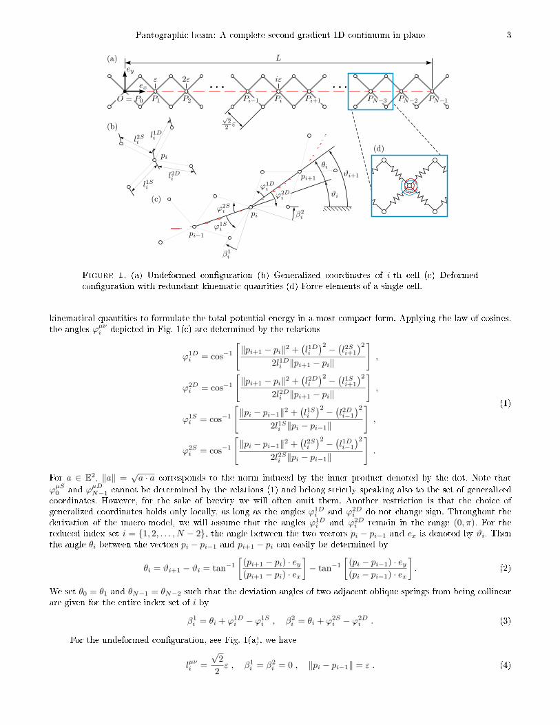
Figure 1. (a) Undeformed con�guration (b) Generalized coordinates of i-th cell (c) Deformedcon�guration with redundant kinematic quantities (d) Force elements of a single cell.

kinematical quantities to formulate the total potential energy in a most compact form. Applying the law of cosines,the angles ϕµνi depicted in Fig. 1(c) are determined by the relations

ϕ1Di = cos−1

[‖pi+1 − pi‖2 +

(l1Di)2 − (l2Si+1

)22l1Di ‖pi+1 − pi‖

],

ϕ2Di = cos−1

[‖pi+1 − pi‖2 +

(l2Di)2 − (l1Si+1

)22l2Di ‖pi+1 − pi‖

],

ϕ1Si = cos−1

[‖pi − pi−1‖2 +

(l1Si)2 − (l2Di−1)2

2l1Si ‖pi − pi−1‖

],

ϕ2Si = cos−1

[‖pi − pi−1‖2 +

(l2Si)2 − (l1Di−1)2


].

(1)

For a ∈ E2, ‖a‖ =√a · a corresponds to the norm induced by the inner product denoted by the dot. Note that

ϕµS0 and ϕµDN−1 cannot be determined by the relations (1) and belong strictly speaking also to the set of generalizedcoordinates. However, for the sake of brevity we will often omit them. Another restriction is that the choice ofgeneralized coordinates holds only locally, as long as the angles ϕ1D

i and ϕ2Di do not change sign. Throughout the

derivation of the macro-model, we will assume that the angles ϕ1Di and ϕ2D

i remain in the range (0, π). For thereduced index set i = {1, 2, . . . , N − 2}, the angle between the two vectors pi − pi−1 and ex is denoted by ϑi. Thenthe angle θi between the vectors pi − pi−1 and pi+1 − pi can easily be determined by

θi = ϑi+1 − ϑi = tan−1[

(pi+1 − pi) · ey(pi+1 − pi) · ex

]− tan−1

[(pi − pi−1) · ey(pi − pi−1) · ex

]. (2)

We set θ0 = θ1 and θN−1 = θN−2 such that the deviation angles of two adjacent oblique springs from being collinearare given for the entire index set of i by

β1i = θi + ϕ1D

i − ϕ1Si , β2

i = θi + ϕ2Si − ϕ2D

i . (3)

For the undeformed con�guration, see Fig. 1(a), we have

lµνi =

√2

2ε , β1

i = β2i = 0 , ‖pi − pi−1‖ = ε . (4)


Letting the summations for i, µ and ν range over the above introduced sets {0, . . . , N − 1}, {1, 2} and {D,S},respectively, the micro-model deformation energy is de�ned as

Eε =kE2

∑i

∑µ,ν

(lµνi −

√2

2ε

)2

+kF2

∑i

∑µ

(βµi )2

(3)=kE2

∑i

∑µ,ν

(lµνi −

√2

2ε

)2

+kF2

∑i

∑µ

[θi + (−1)

µ(ϕµSi − ϕ

µDi

)]2,

(5)

with kE , kF > 0 being the sti�nesses of the extensional and rotational springs, respectively. Boundedness of thedeformation energy, both for the micro-model and for the macro-model is considered throughout this paper. It isworth remarking that besides the rigid body modes also the set of admissible con�gurations de�ned by

lµνi =

√2

2ε , pi = pi−1 +Kex , p0 = P0 , for K ∈

(0,√

2ε), (6)

entails null deformation energy, and is referred to as extensional �oppy mode [12].For the lengths lµνi of the oblique springs, we assume the asymptotic expansion

lµνi =

√2

2ε+ ε2 lµνi + o(ε2) , (7)

where lµνi ∈ R. Inserting assumption (7) into the energy (5) leads to

Eε =kE2

∑i

∑µ,ν

[ε2 lµνi + o(ε2)

]2+kF2

∑i

∑µ

[θi + (−1)

µ (ϕµSi − ϕ

µDi

)]2. (8)

2.2. Micro-macro identi�cation

The slenderness of the discrete system makes it reasonable to aim for a one-dimensional continuum [42] in the limitof vanishing ε. The continuum is then parametrised by the arclength s ∈ [0, L] of the straight segment of length Lconnecting all points Pi. We assume the independent kinematic Lagrangian descriptors of the macro-model to be thefunctions

χ : [0, L]→ E2 , lµν : [0, L]→ R . (9)

The placement function χ places the 1D-continuum into E2 and is best suited to describe the points pi ∈ E2 of thediscrete system on a macro-level. To take into account also the e�ect of changing spring lengths lµνi introduced in

(7), the placement function is augmented by the four micro-strain functions lµν . We thus suggest the identi�cationof the discrete system with a one-dimensional continuum which can be classi�ed as a micromorphic continuum, cf.[43, 44, 45, 46]. It is also convenient to introduce the functions ρ : [0, L] → R+ and ϑ : [0, L] → [0, 2π) in order torewrite the tangent vector �eld χ′ as

χ′(s) = ρ(s) [cosϑ(s)ex + sinϑ(s)ey] , (10)

where prime denotes di�erentiation with respect to the reference arc length s. Thus ρ corresponds to the norm ofthe tangent vector ‖χ′‖ and is referred to as stretch. We explicitly remark that the current curve χ([0, L]) can in

general have a length∫ L0ρ ds di�erent from L, as s is not an arc-length parametrization for χ but for the reference

placement χ0(s) = sex. Introducing moreover the normal vector �eld χ′⊥(s) = ρ(s) [− sinϑ(s)ex + cosϑ(s)ey], beingrotated against χ′(s) about 90◦ in anti-clockwise direction, it can be seen by straight forward computation that

ρ′(s) =χ′(s) · χ′′(s)‖χ′(s)‖

, ϑ′(s) =χ′′(s) · χ′⊥(s)

‖χ′(s)‖2. (11)

In the following ρ′ and ϑ′ are called stretch gradient and material curvature, respectively.For Piola's micro-macro identi�cation we relate the generalized coordinates of the discrete system with the

functions (9) evaluated at si = iε such that

χ(si) = pi , lµν(si) = lµνi . (12)

For the asymptotic identi�cation, we need to expand the energy (8) in ε. To approach this, the expansion of χ isgiven by

χ(si±1) = χ(si)± εχ′(si) +ε2

2χ′′(si) + o(ε2) . (13)


Combining the asymptotic expansion (7) with (12)2, we have

lµνi±1 =

√2

2ε+ lµν(si±1)ε2 + o(ε2) . (14)

Substituting lµν(si±1) = lµν(si) + o(ε0) in (14), we obtain

lµνi±1 =

√2

2ε+ lµν(si)ε

2 + o(ε2) . (15)

In order to further expand (8), we subsequently need to expand the terms θi and ϕµSi − ϕ

µDi up to �rst order. The

detailed expansion is given in the App. A. For θi we have according to (56)

θi = ϑ′(si)ε+ o(ε) . (16)

The di�erences ϕµSi − ϕµDi are given by (63) and (64) as

ϕµSi − ϕµDi =

√2(ρ2)′ + 4

[(l(3−µ)D − l(3−µ)S) + (ρ2 − 1)(lµS − lµD)

]2√

2ρ√

2− ρ2

∣∣∣∣∣s=si

ε+ o(ε) . (17)

Substituting (16) and (17) into (5) together with ρ(si) = ‖χ′(si)‖, we compute the desired expansion of the micro-

model energy Eε as a function of the kinematic descriptors χ and lµν as

Eε =kEε

4

2

∑i

[(l1S)2

+(l1D)2

+(l2S)2

+(l2D)2

+ o(ε0)]s=si

+kF ε

2

2

∑i

[ϑ′ +

−√

2(ρ2)′ − 4[(l2D − l2S)− (ρ2 − 1)(l1D − l1S)

]2√

2ρ√

2− ρ2+ o(ε0)

]2s=si

+kF ε

2

2

∑i

[ϑ′ +

√2(ρ2)′ + 4

[(l1D − l1S) + (ρ2 − 1)(l2S − l2D)

]2√

2ρ√

2− ρ2+ o(ε0)

]2s=si

.

(18)

Let the parameters KE ,KF > 0 be constants, which do not depend on ε. Then these constants are related tothe sti�nesses of each discrete system with micro length scale ε by a scaling law

kE = KEε−κ , kF = KF ε

−η , (19)

with the scaling parameters κ and η. By choosing κ = 3 and η = 1 in (19), observing that∑i o(ε

n) = o(εn−1), theglobal remainder in the energy (18) becomes o(ε0). This remainder speci�es the deformation energy error betweenthe discrete and the continuum model, called discrete-continuum energy error.

2.3. Macro-model

The continuum limit is now obtained by letting ε→ 0 and considering the sum to turn into an integral according to∑i f(si)ε

ε→0−→∫ L0f ds, where f is a real valued function de�ned on [0, L]. Using (18) together with the scaling law

(19) for κ = 3 and η = 1, the deformation energy for the homogenized macro-model becomes

E =

∫ L

0

KE

2

[(l1S)2

+(l1D)2

+(l2S)2

+(l2D)2]

ds

+

∫ L

0

KF

2

[ϑ′ +

−√

2(ρ2)′ − 4[(l2D − l2S)− (ρ2 − 1)(l1D − l1S)

]2√

2ρ√

2− ρ2

]2ds

+

∫ L

0

KF

2

[ϑ′ +

√2(ρ2)′ + 4

[(l1D − l1S) + (ρ2 − 1)(l2S − l2D)

]2√

2ρ√

2− ρ2

]2ds .

(20)

The basic properties of the energy are preserved during the asymptotic process. Both the energy of the micro- and themacro-model (5) and (20), respectively, are invariant under superimposed rigid body motions. Also the extensional

�oppy mode of the discrete model, see (6), transfers to the continuum. Namely, if ρ′ = ϑ′ = lµν = 0, a constant

stretch ρ(s) = K ∈ (0,√

2) can still be present without causing any change in the deformation energy.The above choice of the scaling parameters is such that kF/kE ≈ ε2 asymptotically, as ε → 0. This means that

the extensional springs sti�en much faster than the rotational ones as ε→ 0.Let us de�ne the deformation energy density ψ as the integrand of (20). For the energy to be stationary, the

necessary conditions are obtained by the variation of the deformation energy functional (20). To begin with, we


can also carry out only the variation with respect to lµν . This results in a linear system of 4 equations given by∂ψ/∂lµν = 0 in which lµν are the unknowns. Introducing the abbreviations

C1 =2KF

4KF (ρ2 − 2)−KEρ2, C2 =

2√

2− ρ2KF

KE (ρ2 − 2)− 4KF ρ2, (21)

some necessary conditions for equilibrium are that

lµD =

√2

2ρ[ρ′C1 + (−1)µ−1ϑ′C2

], lµS =

√2

2ρ [−ρ′C1 + (−1)µϑ′C2] . (22)

To solve for lµν , we made use of a computer algebra program. Note that l1D = −l1S and l2D = −l2S . Moreover,if χ′ = ρex with ρ = K ∈ (0,

√2), it follows from (22) that lµν = 0. Hence the independent conditions for the

extensional �oppy mode are that ρ′ = ϑ′ = 0. We further remark that, if ϑ′ = 0, then, from (22), we have thatl1D = l2D and l1S = l2S .

Expanding the brackets in (20), it can readily been seen that the energy contains linear and quadratic terms

in lµν . Asking the coe�cient of (lµν)2 to be strictly positive, the total deformation energy functional (20) is strictlyconvex in lµν . Thus convexity is equivalent to the condition that

KE

KF> 2

(1 +

1

ρ2 − 2− 1

ρ2

). (23)

Since the right hand side of the inequality (23) is strictly negative for ρ ∈ (0,√

2), the inequality is always satis�ed.Accordingly, the set of micro-strains (22) minimizes the deformation energy (20).

By substituting the results (22) into (20), we perform a kinematic reduction resulting in the deformation energyfunctional of the pantographic beam

E =

∫ L

0

KEKF

[ρ2 − 2

ρ2 (KE − 4KF )− 2KEϑ′

2+

ρ2

(2− ρ2) [ρ2 (KE − 4KF ) + 8KF ]ρ′

2]

ds , (24)

which merely depends on the placement function χ. Notice that the complete second gradient χ′′ contributes tothe deformation energy. Indeed, besides the term

(χ′⊥ · χ′′

)being related to the material curvature ϑ′ by means

of (11)1, also the term(χ′ · χ′′

)appears which in turn is related to the stretch gradient ρ′ given by the relation

(24)2. We further remark that the bending sti�ness in (24), i.e. the coe�cient of ϑ′2, does not only depend on thescaled sti�nesses of the elements of the microstructure, but also on ρ. An analogous observation can be done for thecoe�cient of ρ′2. Besides, we notice that the deformation energy (24) is strictly positive for 0 < ρ <

√2 and ϑ′, ρ′

di�erent from zero, as so are the coe�cients of ϑ′ and ρ′ in (24).

In the limit ρ →√

2, the energy (24) reveals a phase transition of the model. While the bending sti�ness, i.e.the coe�cient of ϑ′2, tends to zero, the coe�cient of ρ′2 tends to in�nity. As we assumed boundedness of the energy,the stretch gradient ρ′ must therefore tend to zero. Accordingly, the pantographic beam locally degenerates into amodel of a uniformly extensible cable.

The pantographic beam problem can also be formulated by an augmented energy functional

E = E +

∫ L

0

Λ · [χ′ − ρ(cosϑex + sinϑey)] ds . (25)

in which the �elds χ, ρ and ϑ are regarded as independent kinematic descriptors. We de�ne Ψ as the sum of Ψand the integrand in Eq. (25). The Lagrange multiplier �eld Λ enforces weakly the relations (10). The procedure forobtaining the corresponding Euler-Lagrange equations, not needed for our purposes and thus also not reported here,leads to the following boundary conditions in strong non-dual form

(n) ρ′(0) = 0 ∨ (e) ρ(0) = ρ0 , (n) ρ′(L) = 0 ∨ (e) ρ(L) = ρL

(n) ϑ′(0) = 0 ∨ (e) ϑ(0) = ϑ0 , (n) ϑ′(L) = 0 ∨ (e) ϑ(L) = ϑL .(26)

By (n) and (e) we denote natural and essential boundary conditions, respectively. The conditions for the Lagrangemultiplier �eld is given in strong dual form

Λ(0) · δχ(0) = 0 , Λ(L) · δχ(L) = 0 , (27)

which must hold for any kinematically admissible variation δχ of χ. Let us now make explicit the sets of boundaryconditions entailing ϑ′ = 0 everywhere. To this aim, let us consider the following sets of kinematic quantities evaluatedat the boundary: 1. {χ|0∧L ·ex,with ‖χ0−χL‖ <

√2L}, 2. {χ|0YL ·ex, ρ|0YL <

√2}, and 3. {χ|0∨L ·ex, ρ|0∨L <

√2},

with Y denoting the logical disjunction. If sets 1, 2 or 3 above are �xed as essential boundary conditions we get


ϑ′ = 0, with ϑ being undetermined, unless the condition ϑ|0∨L = ϑ0 is enforced. In particular, �xing sets 1 or 2above results in the extensional �oppy mode.

2.4. Simpli�cations of the energy

The choice κ < 3∨η < 1 in Eq. (19), including κ < 3Yη < 1 or even κ < 3∧η < 1, results in energy functionals whichare rather uninteresting from the macroscopic point of view and we do not intend to pay them further attention.The choice κ = 3 and η = 1 in (19) is such that the energies deriving from all other possible choices can be obtainedfrom the energies (20) and (24) found by means of it.

Case κ < 3∨η < 1. The cases where κ < 3Yη < 1 or even κ < 3∧η < 1 are obtained by computing the limits of(24) for KE → 0YKF → 0 or KE → 0∧KF → 0, respectively. All cases result in a trivial null energy functional whichis rather uninteresting for further analysis. The same trivial cases are achieved when choosing vanishing sti�nesseskE , kF already in the micro-model.

Case κ > 3 ∧ η = 1. This scaling is obtained by computing the limit of (24) by letting KE → ∞. Usingl'Hospital's rule this results in

KF

∫ L

0

(R(ρ)ϑ′

2+

ρ′2

2− ρ2

)ds . (28)

with

R(ρ) =

{0 if ρ =

√2

1 else. (29)

Moreover, this limit process leads to vanishing C1 and C2 in (21) and according to (22) even to vanishing lµν = 0.

Hence, the very same energy can also be computed by just setting lµν = 0 in (20). The deformation energy (28)is given by two additive contributions, the �rst being the deformation energy of the Elastica [47]. Following the

arguments from above, if ρ→√

2, then the continuum behaves locally like a uniformly extensible Elastica.

Note that this scaling captures the case in which the extensional springs become asymptotically so sti� to behavelike rigid links in the limit. In this way, it is also possible to recover the homogenised energy for the pantographicslender system in Fig. 1 with rigid links in place of extensional springs. For a detailed computation we refer to [37].This suggests that interchanging ε→ 0 and KE →∞ to kE →∞ and ε→ 0 leads to the same deformation energy.Also for rigid links, the heuristic homogenisation still gives a o(ε0) discrete-continuum energy error.

Case κ = 3 ∧ η > 1. Carrying out the limit of (24) for KF →∞, again by applying l'Hospital's rule, we get

KE

4

∫ L

0

[2− ρ2

ρ2ϑ′

2+

ρ2

(2− ρ2)2ρ′

2]ds . (30)

The values of lµν expressed in terms of ρ and ϑ which are computed the same way are

lµD = −lµS =

√2

2ρ

[ρ′

2(ρ2 − 2)+ (−1)µ

√2− ρ22ρ2

ϑ′

]. (31)

In a straightforward although a bit cumbersome computation, it can readily be seen that the micro-strains of (31)satisfy the two equalities

2ϑ′ρ√

2√

2− ρ2 = (−1)µ(√

2(ρ2)′ + 4[(lµD − lµS) + (ρ2 − 1)

(l(3−µ)S − l(3−µ)D

)]). (32)

Similar to the previous case, the energy (30) can also be obtained by inserting the results (31) directly into (20).Due to (32), the two last terms of (20) with the factor KF do vanish. In fact, it is the homogenised energy of thepantographic slender system in Fig. 1 in which two opposite oblique springs are enforced to remain collinear.

Case κ > 3 ∧ η > 1. If both KE ,KF → ∞ the microstrains must vanish but also satisfy (31). Consequently,also ρ′ = ϑ′ = 0 allowing the continuum only to deform in the extensional �oppy mode which is characterised by aplacement function such that χ′ = ρex with ρ = K ∈ (0,

√2) together with a null energy functional.

Linearisation. Let the vector valued displacement �eld u be de�ned by u(s) = χ(s)−sex. From Taylor expansionsit follows that ϑ = tan−1(u′ · ey/(1 + u′ · ex)) = u′ · ey + o(‖u′‖) = o(‖u′‖0), ϑ′ = u′′ · ey + o(‖u′‖0), ρ = [(1 + u′ ·ex)2 + (u′ · ey)2]

12 = 1 + u′ · ex + o(‖u′‖) = 1 + o(‖u′‖0), and ρ′ = u′′ · ex + o(‖u′‖0). Hence, the energy of (24) is∫ L

0

[KEKF

KE + 4KF‖u′′‖2 + o(‖u′‖0)

]ds . (33)


For small strain hypothesis the remainder o(‖u′‖0) in Eq. (33) can be neglected. In the limit of KE →∞, (33) leadsto

KF

∫ L

0

‖u′′‖2ds . (34)

This energy corresponds to the deformation energy in (5) with K+ = K− of [12], in which opposite links and therotational spring in between have been considered as a whole by linear and inextensible Euler-Bernoulli beams.

3. Computational aspects

In this section, the solution methods employed for the macro- and micro-model are brie�y recalled.

3.1. Finite element formulation of the macro-model

From the stationarity condition of the energy (25) follows the weak form equation∫ L

0

(∂Ψ

∂ρδρ+

∂Ψ

∂ρ′δρ′ +

∂Ψ

∂ϑ′δϑ′ +

∂Ψ

∂Λ· δΛ +

∂Ψ

∂χ′· δχ′

)ds = 0 , (35)

with δ(·) being kinematically admissible (·), which can then be solved numerically by a �nite element method. Theweak form package of the software COMSOL Multiphysics, which implements standard �nite element techniques (cf.[48, 49]), was used for the discretisation and the subsequent solution procedure. Default settings were set. Essentialboundary conditions, see (26) and (27), were not ful�lled by the basis functions but enforced by additional Lagrangemultipliers. Quadratic Lagrangian polynomials were used as basis functions for the �elds ρ, ϑ and χ. For the �eld Λlinear Lagrangian polynomials were applied. The mesh-size was taken uniformly equal to L/100. Energy convergenceof solutions was successfully checked for the mesh-size tending to 0.

3.2. Micro-model revisited

For solving the discrete micro-model directly and without making any of the hypotheses assumed for the derivation ofthe continuum model, except for the scaling law (19), it is much more convenient to introduce an alternative global,minimal set of generalized coordinates than the one used for the homogenisation. The kinematics of the discretesystem is entirely described by the nodal points pi and p

µνi depicted in Fig. 2 as white �lled circles. the Cartesian

coordinates of the nodes are introduced as 2×1 matrices, i.e. as �row vectors�, in accordance with xi = (pi ·ex, pi ·ey)

and xµSi = (pµSi · ex, pµSi · ey). Hence, the f = 2(3N + 2) generalized coordinates are

q = (x0, · · · , xN−1, x1S0 , · · · , x1SN , x2S0 , · · · , x2SN )T ∈ Rf . (36)

Moreover, we introduce the Boolean connectivity matrices CµSi , CµDi ∈ R4×f de�ned by the relations

qµSi = (xi, xµSi )T = CµSi q qµDi = (xi, x

µSi+1)T = CµDi q . (37)

These are the coordinates required to formulate the energy of the extensional springs. In the energies of the rotationalsprings three points are involved. Accordingly, these coordinates are extracted by the connectivity matrices Cµi ∈ R6×f

de�ned by

q1i = (x1Si , xi, x2Si+1)T = C1

i q q2i = (x2Si , xi, x1Si+1)T = C2

i q . (38)

Figure 2. Nodal points of the micro-model.

Let qe = (x1, y1, x2, y2)T ∈ R4 be the coordinates of two points interconnected by an extensional spring.Introducing the abbreviations ∆x = x2 − x1 and ∆y = y2 − y1, the distance between the two points is

l(qe) =√

∆x2 + ∆y2 =√

(x2 − x1)2 + (y2 − y1)2 . (39)


The derivative with respect to qe is the row vector

∂l

∂qe(qe) =

1

l(qe)(−∆x,−∆y,∆x,∆y) . (40)

For the energy contributions of the rotational springs, we introduce a standard element with three points withcoordinates qr = (x1, y1, x2, y2, x3, y3) ∈ R6. With the abbreviations ∆x1 = x2 − x1, ∆x2 = x3 − x2, ∆y1 = y2 − y1and ∆y2 = y3 − y2, the distances between the respective points are

l1(qr) =√

∆x21 + ∆y21 , l2(qr) =√

∆x22 + ∆y22 , (41)

with the corresponding derivatives

∂l1∂qr

(qr) =1

l1(qr)(−∆x1,−∆y1,∆x1,∆y1, 0, 0) ,

∂l2∂qr

(qr) =1

l2(qr)(0, 0,−∆x2,−∆y2,∆x2,∆y2) .

(42)

The angles between the ex-axis and the vectors ∆x1ex + ∆y1ey and ∆x2ex + ∆y2ey, respectively, are introduced bythe relations

φ1(qr) = tan−1(

∆y1∆x1

), φ2(qr) = tan−1

(∆y2∆x2

)(43)

with the corresponding derivatives

∂φ1∂qr

(qr) =1

l1(qr)2(∆y1,−∆x1,−∆y1,∆x1, 0, 0) ,

∂φ2∂qr

(qr) =1

l2(qr)2(0, 0,∆y2,−∆x2,−∆y2,∆x2) .

(44)

The deformation energy of the micro-model, see (5), is

Eε(q) =∑i

∑µ,ν

kE2

[l(Cµνi q

)−√

2

2ε

]2+kF2

[φ2(Cµi q

)− φ1

(Cµi q

)]2 . (45)

The variation of the deformation energy δEε = (∂Eε/∂q)δq determines the internal generalized forces of themicro-model as [

f intε (q)]T

=∂Eε∂q

=∑i

∑µ,ν

(kE

[l(Cµνi q

)−√

2

2ε

]∂l

∂qe(Cµνi q)Cµνi +

+kF[φ2(Cµi q

)− φ1

(Cµi q

)] [∂φ2∂qr

(Cµi q

)− ∂φ1∂qr

(Cµi q

)]Cµi

).

(46)

Kinematic boundary conditions can be imposed by perfect bilateral constraints 0 = g(q) ∈ Rm with the virtual work

contribution δW c = δgTλ = δqTW (q)λ, where W (q)T = ∂g∂q (q) ∈ Rm×f is the matrix of generalized force directions

and λ ∈ Rm the vector of constraint forces. Together with the generalized internal forces (46), the constrained systemis thus determined by the set of nonlinear equations[

f intε (q) +W (q)λg(q)

]= 0 (47)

which can be solved, at least locally, by a Newton-Raphson iteration scheme.

To compare the numerical results of the micro- and macro-model, beyond the micro-macro identi�cation (12),the following micro-macro correspondences were taken into account

ρ

(si + si−1

2

)↔ ‖pi − pi−1‖

ε, ϑ

(si + si−1

2

)↔ ϑi = tan−1

[(pi − pi−1) · ey(pi − pi−1) · ex

], (48)

where i = {1, . . . , N − 1}. Accepting the stretch ρ and the inclination angle ϑ to be the same for s = 0 and s = ε2 as

well as for s = L and s = L− ε2 , respectively, the micro-macro relations for the boundary conditions are given by

ρ(0)↔ ‖p1 − p0‖ε

, ρ(L)↔ ‖pN−1 − pN−2‖ε

, ϑ(0)↔ ϑ1 , ϑ(L)↔ ϑN−1 . (49)


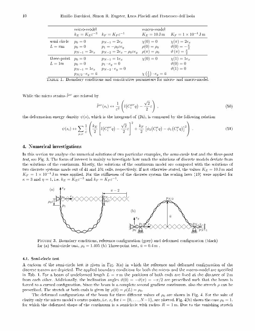
micro-model macro-modelkE = KEε

−3 kF = KF ε−1 KE = 10 J m KF = 1× 10−4 J m

semi-circle p0 = 0 pN−1 = 2ex χ(0) = 0 χ(π) = 2exL = πm p0 = 0 p1 = −ρ0εey ρ(0) = ρ0 ϑ(0) = −π2

pN−1 = 2ex pN−2 = 2ex − ρ0εey ρ(π) = ρ0 ϑ (π) = π2

three-point p0 = 0 pN−1 = 1ex χ(0) = 0 χ(1) = 1exL = 1m p0 = 0 p1 · ey = 0 ϑ(0) = 0

pN−1 = 1ex pN−2 · ey = 0 ϑ(1) = 0pN/2 · ey = u χ

(12

)· ey = u

Table 1. Boundary conditions and constitutive parameters for micro- and macro-model.

While the micro-strains lµν are related by

lµν(si)↔1

ε2

(l(Cµνi q

)−√

2

2ε

), (50)

the deformation energy density ψ(s), which is the integrand of (24), is compared by the following relation

ψ(si)↔∑µ,ν

1

ε

kE2

[l(Cµνi q

)−√

2

2ε

]2+kF2

[φ2(Cµi q

)− φ1

(Cµi q

)]2 . (51)

4. Numerical investigations

In this section we analyse the numerical solutions of two particular examples, the semi-circle test and the three-pointtest, see Fig. 3. The focus of interest is mainly to investigate how much the solutions of discrete models deviate fromthe solutions of the continuum. Mostly, the solutions of the continuum model are compared with the solutions oftwo discrete systems made out of 41 and 101 cells, respectively. If not otherwise stated, the values KE = 10 J m andKF = 1× 10−4 J m were applied. For the sti�nesses of the discrete system the scaling laws (19) were applied forκ = 3 and η = 1, i.e. kE = KEε

−3 and kF = KF ε−1.

Figure 3. Boundary conditions, reference con�guration (grey) and deformed con�guration (black)for (a) Semi-circle test, ρ0 = 1.405 (b) Three-point test, u = 0.4 m .

4.1. Semi-circle test

A cartoon of the semi-circle test is given in Fig. 3(a) in which the reference and deformed con�guration of thediscrete system are depicted. The applied boundary conditions for both the micro- and the macro-model are speci�edin Tab. 1. For a beam of undeformed length L = πm the positions of both ends are �xed at the distance of 2 mfrom each other. Additionally, the inclination angles ϑ(0) = −ϑ(π) = −π/2 are prescribed such that the beam isforced to a curved con�guration. Since the beam is a complete second gradient continuum, also the stretch ρ can beprescribed. The stretch at both ends is given by ρ(0) = ρ(L) = ρ0.

The deformed con�gurations of the beam for three di�erent values of ρ0 are shown in Fig. 4. For the sake ofclarity only the micro-model's centre points, i.e. xi for i = {0, . . . , N−1}, are plotted. Fig. 4(b) shows the case ρ0 = 1,for which the deformed shape of the continuum is a semicircle with radius R = 1 m. Due to the vanishing stretch


gradient along the beam, i.e. ρ′ = 0 as it can be seen in Fig. 5(b), the total length of the beam remains equal to π m.Moreover, the material curvature takes uniformly the value ϑ′ = 1/R = 1m−1. This corresponds with the solutionof the Elastica for the same boundary conditions. Note that the inextensibility condition inherently contained in theformulation of the Elastica does not allow to prescribe another value of the stretch than ρ = 1. The slight deviationsof the discrete systems from the circle is mainly due to the discrete �approximation� of the boundary conditions.

In Fig. 4(a) and (c), the in�uence of the prescribed stretch becomes apparent. While for ρ0 < 1 the beam isshortened, for ρ0 > 1 the beam is elongated. Besides the fact that it would have been a rather di�cult task to �nda deformation energy (24) without homogenization, another convenient feature comes along with that procedure. Itallows to develop a more intuitive understanding of boundary conditions which appear in higher gradient continua.According to Tab. 1, the boundary condition of the micro-model which corresponds to the prescription of the stretchis realized by �xing the distance between two adjacent centre points. If the distance between two adjacent points isincreased with respect to the reference con�guration, as in Fig. 3(a), an accordion-like (homogeneous) extension isobserved in the micro-model. Moreover, the boundary conditions of both stretch ρ and inclination angle ϑ e�ect overa much larger distance than placement boundary conditions. This is precisely the characteristics contained in highergradient continua.

Figure 4. Semi-circle test. Deformed con�gurations of micro- and macro-model for (a) ρ0 = 0.5,(b) ρ0 = 1, and (c) ρ0 = 1.405.

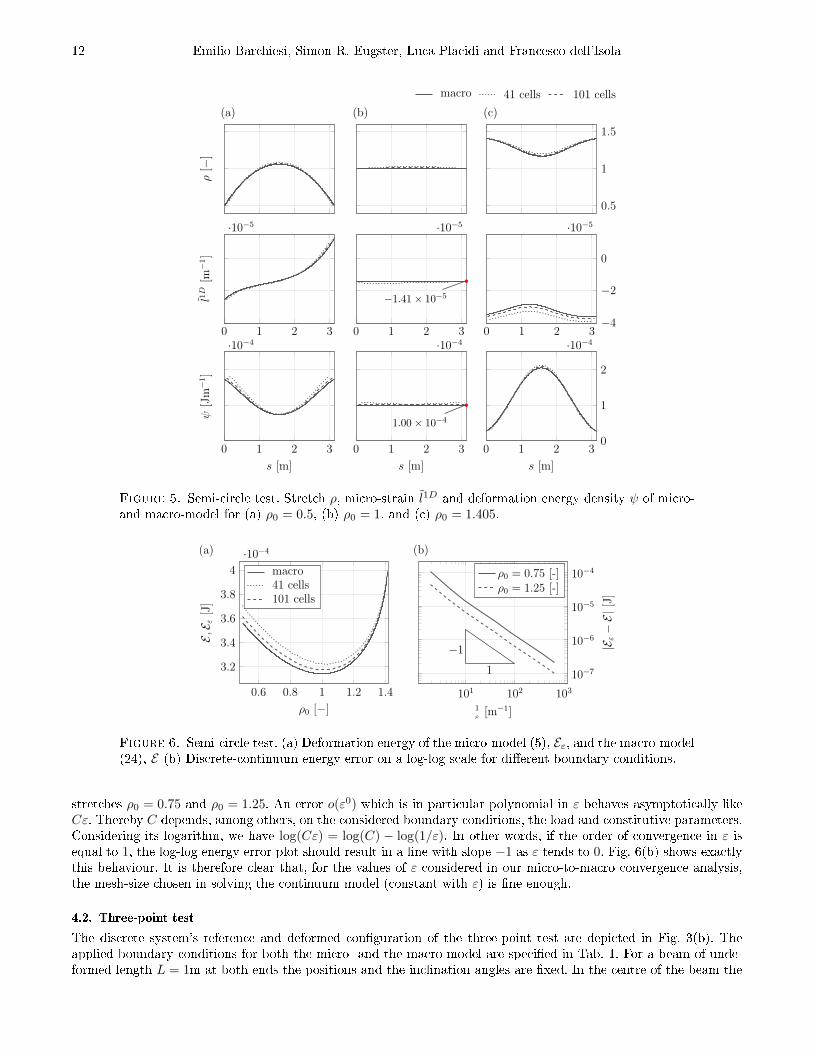
In Fig. 5 the micro-stretch l1D, the stretch ρ and the deformation energy density ψ are plotted for di�erentvalues of ρ0. The symmetry in the boundary conditions is re�ected in the obtained curves parametrised by s ∈ [0, π].We have the symmetry ρ(s) = ρ(π−s) and ϑ(s) = −ϑ(π−s) (not plotted). Consequently, the stretch gradient and thematerial curvature are odd and even functions shifted by π, respectively, i.e. ρ′(s) = −ρ′(π−s) and ϑ′(s) = ϑ′(π−s).Since all these kinematical quantities appear quadratically in (24), also the deformation energy density ψ is an even

function shifted by π. Furthermore, (22) implies that l1ν(s) = −l2ν(π − s). Accordingly, only the micro-stretch l1D

is plotted in Fig. 5.As discussed before, for ρ0 = 1, the stretch ρ and the material curvature ϑ′ are uniformly equal to 1. It follows

then immediately from (22) and (24) that the micro-stretch and the deformation energy density take the values

l1D = −√

2KF

KE + 4KF= −1.41× 10−5 m−1 , ψ =

KEKF

KE + 4KF= 1× 10−4 Jm−1 , (52)

which is indeed the case when considering Fig. 5.In Fig. 6(a), the deformation energies are given as ρ0 increases. While for the continuum model the deformation

energy attains a minimum at ρ0 = 1, this does not hold true for the micro-model, whose deformation energies attaina minimum at ρ0 > 1. The simulation were performed to come as close to the limit case

√2 = 1.41 as possible.

The Lagrange multipliers satisfying the boundary conditions for ρ can be considered as double forces acting at theends of the beam. Their resultant value can be obtained by Castigliano's theorem by taking the derivative of thedeformation energy with respect to ρ, i.e. considering the inclination angles of the curves in Fig. 6(a). The closer

we come to√

2 the steeper the curve gets and the double forces tend to in�nity. In this extreme regions numericalanalysis gets di�cult.

After a qualitative comparison between macro- and micro-model, we quantify the error by the absolute valueof the di�erence between the deformation energy of the macro-model E and the micro-model Eε. Within the micro-macro identi�cation procedure, we accepted a discrete-continuum energy error o(ε0), i.e. of order 1 in ε. Therefore,for a meaningful analysis the energy error in the �nite element solution of the macro-model (and/or that possiblydone when considering the small-strain assumption) should be o(ε), so to be negligible with respect to the discrete-continuum energy error. In Fig. 6(b) the discrete-continuum energy error is plotted against 1/ε for the boundary


Figure 5. Semi-circle test. Stretch ρ, micro-strain l1D and deformation energy density ψ of micro-and macro-model for (a) ρ0 = 0.5, (b) ρ0 = 1, and (c) ρ0 = 1.405.

Figure 6. Semi-circle test. (a) Deformation energy of the micro-model (5), Eε, and the macro-model(24), E (b) Discrete-continuum energy error on a log-log scale for di�erent boundary conditions.

stretches ρ0 = 0.75 and ρ0 = 1.25. An error o(ε0) which is in particular polynomial in ε behaves asymptotically likeCε. Thereby C depends, among others, on the considered boundary conditions, the load and constitutive parameters.Considering its logarithm, we have log(Cε) = log(C) − log(1/ε). In other words, if the order of convergence in ε isequal to 1, the log-log energy error plot should result in a line with slope −1 as ε tends to 0. Fig. 6(b) shows exactlythis behaviour. It is therefore clear that, for the values of ε considered in our micro-to-macro convergence analysis,the mesh-size chosen in solving the continuum model (constant with ε) is �ne enough.

4.2. Three-point test

The discrete system's reference and deformed con�guration of the three-point test are depicted in Fig. 3(b). Theapplied boundary conditions for both the micro- and the macro-model are speci�ed in Tab. 1. For a beam of unde-formed length L = 1m at both ends the positions and the inclination angles are �xed. In the centre of the beam the


vertical displacement u is prescribed. We remark that the small strain approximation is for each point (to di�erentextents) as less valid as u increases and, in what follows, we have been using the deformation energy (24).

macro 41 cells 101 cells

0 0.2 0.4 0.6 0.8 1

0

0.1

0.2

u · ex + s [m]

u·e

y[m

]

(a)

0 0.2 0.4 0.6 0.8 1

1.06

1.08

1.1

1.12

s [m]

ρ[−

]

(b)

0 0.2 0.4 0.6 0.8 1

−0.5

0

0.5

s [m]

ϑ[−

]

(c)

0 0.2 0.4 0.6 0.8 1

0

1

2

·10−3

s [m]

ψ[Jm

−1]

(d)

Figure 7. Three-point test. Micro- and macro model for u = 0.2 m (a) Deformed con�guration (b)Stretch ρ (c) Inclination angle ϑ (d) Deformation energy density ψ.

In Fig. 7 the deformed con�guration, the stretch ρ, the inclination angle ϑ and the deformation energy densityψ are plotted for u = 0.2 m. Also here, the symmetry in the boundary conditions is re�ected in the obtained curvesparametrised by s ∈ [0, 1]. We have the symmetries ρ(s) = ρ(1 − s) and ϑ(s) = −ϑ(1 − s). According to the samearguments given in the semi-circle test, the deformation energy density (24) must be an even function shifted by0.5. Fig. 7(d) shows that this property is ful�lled by both the micro- and the macro-model. Due to the symmetries

appearing also in the micro-stretches, in Fig. 8 only the micro-stretch l1D is plotted for di�erent values of u.

Figure 8. Three-point test. Micro-stretch l1D of the micro- and macro-model for (a) u = 0.1 m (b)u = 0.25 m (c) u = 0.4 m.

In Figs. 9 the stretches ρ and the deformed con�gurations of the continuum are plotted for di�erent values ofu. The remarkable phenomena appearing in this test is that for u = 0.4408, one has ρ ≈

√2 and ρ′ ≈ 0 everywhere.

Hence, if u is tending to some value slightly greater than 0.4408 m, then ρ tends to√

2. This is the value, wherethe model undergoes a phase transition from a pantographic beam to a uniformly extensible cable. Even though this


phase transition can be interpreted from the deformation energy (24) it is not directly captured by the continuummodel due to the restrictions made in the choice of minimal coordinates. The discrete model could overcome thisproblem. However, as we will see below, stability problems become an issue for which reason the numerical solutionprocedure needs to be extended.

Figure 9. Three-point test. (a) Stretch ρ (b) Deformed con�guration of macro-model.

In Fig. 10 the deformation energy for u = 0.2 m as KE and KF increase. The red lines indicate the totaldeformation energy as the kinematic constraints corresponding to KE → ∞ and to KF → ∞ are enforced. Thesevalues are asymptotes for the black curves, indicating that the energy of the macro-model in (24), as KE → ∞,converges to that in (28) and the energy of the micro-model (5) converges to that of the same system with extensionalsprings replaced by rigid links. Let us consider Fig. 10(a). For ε→ 0, the asymptotes (red lines) related to the micro-model converge to that of the macro-model, as well as the black curves do. Therefore, in agreement to what has beensuggested by heuristic analytical derivations, Fig. 10(a) indicates that interchanging ε→ 0 and KE →∞ to kE →∞and ε → 0 leads to the same deformation energy. Similar conclusions can be drawn for KF → ∞ and kF → ∞,referring to Fig. 10(b).

macro 41 cells 101 cells 501 cells 1001 cells

0 5 10 156.8

7

7.2

7.4

·10−4

6.892 · 10−4

KE [Jm]

E,E ε

[J]

(a)

0 100 200 30010

11

12

11.195

KF [Jm]

E,E ε

[J]

(b)

Figure 10. Three-point test. Deformation energy of the micro-model (5), Eε, and the macro-model(24), E , for u = 0.2 m. The red lines indicate the deformation energies for cases in which the kinematicconstraints corresponding to (a) kE →∞,KE →∞ or (b) kF →∞,KF →∞ are enforced.

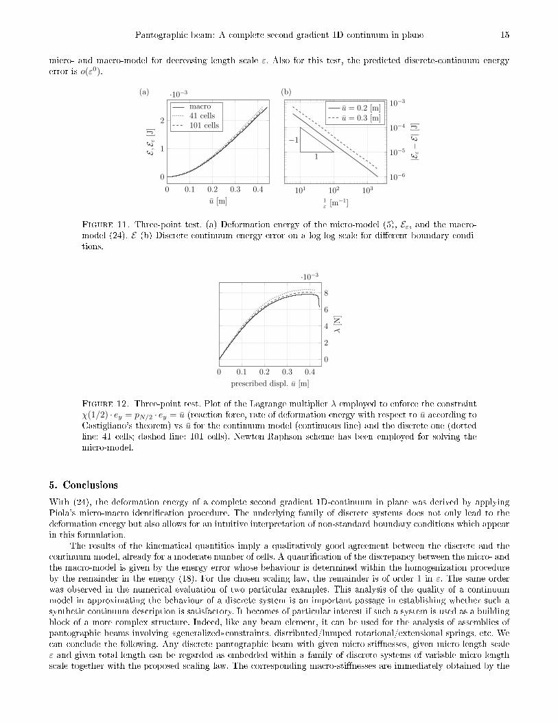
In Fig. 11(a) the deformation energy is plotted as the prescribed displacement u increases. According to Cas-tigliano's theorem the required pulling force in the centre of the beam corresponds with the slope of the deformationenergy graph ∂E/∂u, and in turn to the Lagrange multiplier employed to enforce the corresponding kinematic con-straint. The required change of force to pull the beam further (proportional � with positive ratio � to the sti�ness)is positive and decreasing, tending to zero for u approaching 0.405 m (see Fig. 12). Therefore, the Newton-Raphsonscheme does not converge and the simulation can not go further. Arclength methods such as the Riks' arc-lengthmethod [50] have to be implemented in order to overcome this problem which is beyond the scope of this article.The continuum model could be instead solved for values of u greater than 0.405 m, showing negative and decreasingsti�ness blowing up to −∞ for u approaching 0.4408 m. Fig. 11(b) shows on a log-log scale the energy error between


micro- and macro-model for decreasing length scale ε. Also for this test, the predicted discrete-continuum energyerror is o(ε0).

Figure 11. Three-point test. (a) Deformation energy of the micro-model (5), Eε, and the macro-model (24), E (b) Discrete-continuum energy error on a log-log scale for di�erent boundary condi-tions.

??

0 0.1 0.2 0.3 0.4

0

2

4

6

8

·10−3

prescribed displ. u [m]

λ[N

]

Figure 12. Three-point test. Plot of the Lagrange multiplier λ employed to enforce the constraintχ(1/2) · ey = pN/2 · ey = u (reaction force, rate of deformation energy with respect to u according toCastigliano's theorem) vs u for the continuum model (continuous line) and the discrete one (dottedline: 41 cells; dashed line: 101 cells). Newton-Raphson scheme has been employed for solving themicro-model.

5. Conclusions

With (24), the deformation energy of a complete second gradient 1D-continuum in plane was derived by applyingPiola's micro-macro identi�cation procedure. The underlying family of discrete systems does not only lead to thedeformation energy but also allows for an intuitive interpretation of non-standard boundary conditions which appearin this formulation.

The results of the kinematical quantities imply a qualitatively good agreement between the discrete and thecontinuum model, already for a moderate number of cells. A quanti�cation of the discrepancy between the micro- andthe macro-model is given by the energy error whose behaviour is determined within the homogenization procedureby the remainder in the energy (18). For the chosen scaling law, the remainder is of order 1 in ε. The same orderwas observed in the numerical evaluation of two particular examples. This analysis of the quality of a continuummodel in approximating the behaviour of a discrete system is an important passage in establishing whether such asynthetic continuum description is satisfactory. It becomes of particular interest if such a system is used as a buildingblock of a more complex structure. Indeed, like any beam element, it can be used for the analysis of assemblies ofpantographic beams involving �generalized�constraints, distributed/lumped rotational/extensional springs, etc. Wecan conclude the following. Any discrete pantographic beam with given micro-sti�nesses, given micro-length scaleε and given total length can be regarded as embedded within a family of discrete systems of variable micro-lengthscale together with the proposed scaling law. The corresponding macro-sti�nesses are immediately obtained by the


scaling law. We then know that the quality in terms of energy of the continuum to represent the discrete systembehaves linearly in the micro-length scale ε. Finally, the methodology and results of the present paper should serveas prototypes for the asymptotic analysis of more complex systems, especially for a class of bi-dimensional structureswhich generalises pantographic fabrics (cf. [38]).Acknowledgements. Authors thank P. Seppecher for insightful discussions.

Appendix A

The terms θi and ϕµSi − ϕ

µDi are expanded up to �rst order by using the de�nitions (1) and (2) together with the

expansions (13) and (14). According to (12) and (13) the vectors between two adjacent points are

pi+1 − pi = ε[χ′(si) +

ε

2χ′′(si) + o(ε)

], pi − pi−1 = ε

[χ′(si)−

ε

2χ′′(si) + o(ε)

]. (53)

The arguments of the tan−1 in (2) can be written as functions of ε

hi+1(ε) =(pi+1 − pi) · ey(pi+1 − pi) · ex

(53)1=χ′(si) · ey + ε

2χ′′(si) · ey + o(ε)

χ′(si) · ex + ε2χ′′(si) · ex + o(ε)

,

hi(ε) =(pi − pi−1) · ey(pi − pi−1) · ex

(53)2=χ′(si) · ey − ε

2χ′′(si) · ey + o(ε)

χ′(si) · ex − ε2χ′′(si) · ex + o(ε)

.

(54)

It can readily be seen that hi(0) = hi+1(0) = [χ′(si) · ey] / [χ′(si) · ex]. Moreover

h′i+1(0) = −h′i(0) =1

2[χ′ · ex]2[(χ′′ · ey)(χ′ · ex)− (χ′′ · ex)(χ′ · ey)]

∣∣∣∣s=si

=1

2[χ′ · ex]2χ′′ · (ey ⊗ ex − ex ⊗ ey) · χ′

∣∣∣∣s=si

=χ′′(si) · χ′⊥(si)

2 [χ′(si) · ex]2 .

(55)

For a real valued function h(ε), we can expand tan−1(h(ε)) = tan−1(h(0)) + h′(0)1+h(0)2 ε+ o(ε). Since hi(0) = hi+1(0),

the �rst terms in the Taylor series of both tan−1 expressions in (2) coincide and we obtain

θi =

[1

1 + hi+1(0)2h′i+1(0)− 1

1 + hi(0)2h′i(0)

]ε+ o(ε)

(55)=

1

1 +[χ′(si)·eyχ′(si)·ex

]2 χ′′(si) · χ′⊥(si)

[χ′(si) · ex]2 ε+ o(ε)

=χ′′(si) · χ′⊥(si)

‖χ′(si)‖2ε+ o(ε)

(11)= ϑ′(si)ε+ o(ε) .

(56)

For the expansion (1), we �rst require the expansion of the norm of a vector valued function a(ε), i.e. ‖a(ε)‖ =

‖a(0)‖+ a(0)·a′(0)‖a(0)‖ ε+o(ε). Taking a(ε) to be the expansions appearing in the squared brackets of (53) and considering

that ρ(s) = ‖χ′(s)‖, we can write

‖pi±1 − pi‖ = ε

[‖χ′(si)‖ ±

χ′(si) · χ′′(si)‖χ′(si)‖

ε

2+ o(ε)

]= ε

[ρ(si)± ρ′(si)

ε

2+ o(ε)

]. (57)

Consequently, the expansion of the squared expression of (57) is

‖pi±1 − pi‖2 = ε2[‖χ′‖2 ± (χ′ · χ′′)ε+ o(ε)

]s=si

= ε2[ρ2 ± ρρ′ε+ o(ε)

]s=si

. (58)

Using (15), (57) and (58) in the argument of cos−1 of (1)2, we can compute

h1S(ε) =‖pi − pi−1‖2 + (l1Si )2 − (l2Di−1)2


=ε2[ρ2 − ρρ′ε+

√2ε(l1S − l2D) + o(ε)

]ε22[√

22 + l1Sε+ o(ε)

] [ρ− ρ′ ε2 + o(ε)

]∣∣∣∣∣∣s=si

=ρ2 + ε

[√2(l1S − l2D)− ρρ′

]+ o(ε)

√2ρ+ ε

(2l1Sρ−

√22 ρ′)

+ o(ε)

∣∣∣∣∣∣s=si

.

(59)


Similarly, the expansions of the arguments of cos−1 appearing in (1)1,3,4 are

h1D(ε) =ρ2 + ε

[√2(l1D − l2S) + ρρ′

]+ o(ε)

√2ρ+ ε

(2l1Dρ+

√22 ρ′)

+ o(ε)

∣∣∣∣∣∣s=si

(60)

h2S(D)(ε) =ρ2 + ε

[√2(l2S(D) − l1D(S))− ρρ′

]+ o(ε)

√2ρ+ ε

(2l2S(D)ρ−

√22 ρ′)

+ o(ε)

∣∣∣∣∣∣s=si

(61)

All functions are of the form hµν(ε) = [a+ εbµν + o(ε)] / [c+ εdµν + o(ε)] with hµν(0) = a/c and (hµν)′(0) =(bµνc− dµνa)/c2. The angles ϕµνi can thus be expanded as

ϕµνi = cos−1 [hµν(0)]− ε√1− hµν(0)2

(hµν)′(0) + o(ε) . (62)

Expanding ϕµSi − ϕµDi with the help of (62), the �rst term thereof cancels. Inserting the derivative with respect to

ε evaluated at ε = 0 of (59) and (60)1, we obtain

ϕ1Si − ϕ1D

i =

√2ρ[2ρρ′ +

√2(l1D − l2S + l2D − l1S)

]+ ρ2

[2ρ(l1S − l1D)−

√2ρ′]

2ρ2√

1− ρ2

2

∣∣∣∣∣∣s=si

ε+ o(ε)

=

√22 ρρ

′ + (l2D − l2S) + (ρ2 − 1)(l1S − l1D)

ρ√

1− ρ2

2

∣∣∣∣∣∣s=si

ε+ o(ε) . (63)

In the same manner we obtain the expansion for the di�erence in angles of the oblique springs indexed by µ = 2.Moreover, we manipulate the expression slightly to get rid of the fractions within the nominator and denominatorwhich results in

ϕ2Si − ϕ2D

i =

√2(ρ2)′ + 4

[(l1D − l1S) + (ρ2 − 1)(l2S − l2D)

]2√

2ρ√

2− ρ2

∣∣∣∣∣s=si

ε+ o(ε) . (64)

References

[1] Harrison P. 2016 Modelling the forming mechanics of engineering fabrics using a mutually constrained pantographic beamand membrane mesh. Composites Part A: Applied Science and Manufacturing 81, 145�157.

[2] Andreaus U, dell'Isola F, Giorgio I, Placidi L, Lekszycki T, Rizzi N. 2016 Numerical simulations of classical problems intwo-dimensional (non) linear second gradient elasticity. International Journal of Engineering Science 108, 34�50.

[3] Au�ray N, Dirrenberger J, Rosi G. 2015 A complete description of bi-dimensional anisotropic strain-gradient elasticity.International Journal of Solids and Structures 69, 195�206.

[4] Battista A, Rosa L, dell'Erba R, Greco L. 2016 Numerical investigation of a particle system compared with �rst and secondgradient continua: Deformation and fracture phenomena. Mathematics and Mechanics of Solids p. 1081286516657889.

[5] Steigmann DJ. 1996 The variational structure of a nonlinear theory for spatial lattices. Meccanica 31, 441�455.

[6] dell'Isola F, Lekszycki T, Pawlikowski M, Grygoruk R, Greco L. 2015 Designing a light fabric metamaterial being highlymacroscopically tough under directional extension: �rst experimental evidence. Zeitschrift für angewandte Mathematikund Physik 66, 3473�3498.

[7] Giorgio I, Della Corte A, dell'Isola F, Steigmann DJ. 2016 Buckling modes in pantographic lattices. Comptes rendusMecanique 344, 487�501.

[8] Giorgio I, Della Corte A, dell'Isola F. 2017 Dynamics of 1D nonlinear pantographic continua. Nonlinear Dynamics 88,21�31.

[9] Turco E, Misra A, Pawlikowski M, dell'Isola F, Hild F. 2018 Enhanced Piola�Hencky discrete models for pantographicsheets with pivots without deformation energy: Numerics and experiments. International Journal of Solids and Structures.

[10] Turco E, Golaszewski M, Cazzani A, Rizzi N. 2016a Large deformations induced in planar pantographic sheets by loadsapplied on �bers: experimental validation of a discrete Lagrangian model.Mechanics Research Communications 76, 51�56.

[11] Turco E, Barcz K, Pawlikowski M, Rizzi N. 2016b Non-standard coupled extensional and bending bias tests for planarpantographic lattices. Part I: numerical simulations. Zeitschrift für angewandte Mathematik und Physik 67, 122.

[12] Alibert JJ, Seppecher P, dell'Isola F. 2003 Truss modular beams with deformation energy depending on higher displacementgradients. Mathematics and Mechanics of Solids 8, 51�73.


[13] Andreaus U, Spagnuolo M, Lekszycki T, Eugster SR A Ritz approach for the static analysis of planar pantographicstructures modeled with nonlinear Euler�Bernoulli beams. Continuum Mechanics and Thermodynamics pp. 1�21.

[14] Spagnuolo M, Barcz K, Pfa� A, dell'Isola F, Franciosi P. 2017 Qualitative pivot damage analysis in aluminum printedpantographic sheets: numerics and experiments. Mechanics Research Communications 83, 47�52.

[15] Scerrato D, Zhurba Eremeeva IA, Lekszycki T, Rizzi NL. 2016 On the e�ect of shear sti�ness on the plane deformationof linear second gradient pantographic sheets. ZAMM-Journal of Applied Mathematics and Mechanics/Zeitschrift fürAngewandte Mathematik und Mechanik 96, 1268�1279.

[16] Cuomo M, dell'Isola F, Greco L. 2016 Simpli�ed analysis of a generalized bias test for fabrics with two families ofinextensible �bres. Zeitschrift für angewandte Mathematik und Physik 67.

[17] dell'Isola F, Giorgio I, Pawlikowski M, Rizzi NL. 2016 Large deformations of planar extensible beams and pantographiclattices: heuristic homogenization, experimental and numerical examples of equilibrium. Proc. R. Soc. A 472.

[18] Misra A, Lekszycki T, Giorgio I, Ganzosch G, Müller WH, dell'Isola F. 2018 Pantographic metamaterials show atypicalPoynting e�ect reversal. Mech. Res. Commun. 89, 6�10.

[19] Eremeyev VA, dell'Isola F, Boutin C, Steigmann D. 2017 Linear pantographic sheets: existence and uniqueness of weaksolutions. Journal of Elasticity pp. 1�22.

[20] Placidi L, Barchiesi E, Turco E, Rizzi N. 2016a A review on 2D models for the description of pantographic fabrics.Zeitschrift für angewandte Mathematik und Physik 67(5).

[21] Placidi L, Andreaus U, Giorgio I. 2016b Identi�cation of two-dimensional pantographic structure via a linear D4 or-thotropic second gradient elastic model. Journal of Engineering Mathematics pp. 1�21.

[22] Giorgio I. 2016 Numerical identi�cation procedure between a micro-Cauchy model and a macro-second gradient modelfor planar pantographic structures. Zeitschrift für angewandte Mathematik und Physik 67(4).

[23] Babu²ka I. 1976 Homogenization approach in engineering. In Computing methods in applied sciences and engineering pp.137�153. Springer.

[24] Allaire G. 1992 Homogenization and two-scale convergence. SIAM Journal on Mathematical Analysis 23, 1482�1518.

[25] Tartar L. 2009 The general theory of homogenization: a personalized introduction vol. 7. Springer Science & BusinessMedia.

[26] Yu W, Tang T. 2009 Variational asymptotic method for unit cell homogenization. In Advances in Mathematical Modelingand Experimental Methods for Materials and Structures pp. 117�130. Springer.

[27] Golaszewski M, Grygoruk R, Giorgio I, Laudato M, Di Cosmo F. 2018 Metamaterials with relative displacements in theirmicrostructure: technological challenges in 3D printing, experiments and numerical predictions. Continuum Mechanicsand Thermodynamics pp. 1�20.

[28] Yang T, Bellouard Y. 2015 3D electrostatic actuator fabricated by non-ablative femtosecond laser exposure and chemicaletching. In MATEC Web of Conferences vol. 32. EDP Sciences.

[29] Koch F, Lehr D, Schönbrodt O, Glaser T, Fechner R, Frost F. 2018 Manufacturing of highly-dispersive, high-e�ciencytransmission gratings by laser interference lithography and dry etching. Microelectronic Engineering 191, 60�65.

[30] Yamada K, Yamada M, Maki H, Itoh K. 2018 Fabrication of arrays of tapered silicon micro-/nano-pillars by metal-assistedchemical etching and anisotropic wet etching. Nanotechnology 29, 28LT01.

[31] Larsson MP. 2006 Arbitrarily pro�led 3D polymer MEMS through Si micro-moulding and bulk micromachining. Micro-electronic engineering 83, 1257�1260.

[32] Milton G, Briane M, Harutyunyan D. 2017a On the possible e�ective elasticity tensors of 2-dimensional and 3-dimensionalprinted materials. Math. and Mech. of Comp. Sys. 5, 41�94.

[33] Milton G, Harutyunyan D, Briane M. 2017b Towards a complete characterization of the e�ective elasticity tensors ofmixtures of an elastic phase and an almost rigid phase. Mathematics and Mechanics of Complex Systems 5, 95�113.

[34] Abdoul-Anziz H, Seppecher P. 2018 Strain gradient and generalized continua obtained by homogenizing frame lattices.Mathematics and Mechanics of Complex Systems.

[35] Barchiesi E, Spagnuolo M, Placidi L. 2018 Mechanical metamaterials: a state of the art. Mathematics and Mechanics ofSolids.

[36] Di Cosmo F, Laudato M, Spagnuolo M. 2018 Acoustic Metamaterials Based on Local Resonances: Homogenization,Optimization and Applications. In Generalized Models and Non-classical Approaches in Complex Materials 1 pp. 247�274. Springer.

[37] Barchiesi E, dell'Isola F, Laudato M, Placidi L, Seppecher P. 2018 A 1D Continuum Model for Beams with PantographicMicrostructure: Asymptotic Micro-Macro Identi�cation and Numerical Results. In Advances in Mech. of Microstruct.Media and Struct. pp. 43�74. Springer.

[38] Seppecher P, Alibert JJ, dell'Isola F. 2011 Linear elastic trusses leading to continua with exotic mechanical interactions.In J. of Physics: Conference Series vol. 319 pp. 12�18. IOP Publishing.


[39] Alibert JJ, Della Corte A, Giorgio I, Battista A. 2017 Extensional Elastica in large deformation as Γ-limit of a discrete1D mechanical system. Z. Angew. Math. Phys. 68, 42.

[40] Eremeyev VA, Pietraszkiewicz W. 2004 The nonlinear theory of elastic shells with phase transitions. Journal of Elasticity74, 67�86.

[41] Eugster SR, Glocker C. 2017 On the notion of stress in classical continuum mechanics. Mathematics and Mechanics ofComplex Systems 5, 299�338.

[42] Steigmann D, Faulkner M. 1993 Variational theory for spatial rods. Journal of Elasticity 33, 1�26.

[43] Germain P. 1973 The Method of Virtual Power in Continuum Mechanics. Part 2: Microstructure. SIAM Journal onApplied Mathematics 25, 556�575.

[44] Forest S, Sievert R. 2006 Nonlinear microstrain theories. International Journal of Solids and Structures 43, 7224 � 7245.Size-dependent Mechanics of Materials.

[45] Eremeyev VA, Lebedev LP, Altenbach H. 2012 Foundations of micropolar mechanics. Springer Science & Business Media.

[46] Altenbach H, Bîrsan M, Eremeyev VA. 2013 Cosserat-type rods. In Generalized Continua from the Theory to EngineeringApplications pp. 179�248. Springer.

[47] Spagnuolo M, Andreaus U. 2018 A targeted review on large deformations of planar elastic beams: extensibility, distributedloads, buckling and post-buckling. Mathematics and Mechanics of Solids.

[48] Abali B, Müller W, Eremeyev V. 2015 Strain gradient elasticity with geometric nonlinearities and its computationalevaluation. Mechanics of Advanced Materials and Modern Processes 1, 4.

[49] Abali BE, Müller WH, dell'Isola F. 2017 Theory and computation of higher gradient elasticity theories based on actionprinciples. Archive of Applied Mechanics 87, 1495�1510.

[50] Riks E. 1979 An incremental approach to the solution of snapping and buckling problems. International journal of solidsand structures 15, 529�551.

Emilio Barchiesi (corr. auth.)Dipartimento di Ingegneria Strutturale e Geotecnica, Università degli Studi di Roma �La Sapienza�, ItalyInternational Research Center M&MoCS, Università degli Studi dell'Aquila, Italye-mail: [email protected]

Simon R. EugsterInstitute for Nonlinear Mechanics, University of Stuttgart, Germany

Luca PlacidiFacoltà di Ingegneria, Università Telematica Internazionale UNINETTUNO, ItalyInternational Research Center M&MoCS, Università degli Studi dell'Aquila, Italy

Francesco dell'IsolaDipartimento di Ingegneria Civile, Edile-Architettura e Ambientale, Università degli Studi dell'Aquila, ItalyDipartimento di Ingegneria Strutturale e Geotecnica, Università degli Studi di Roma �La Sapienza�, ItalyInternational Research Center M&MoCS, Università degli Studi dell'Aquila, Italy

pantographic beam: a complete second gradient 1d-continuum

Documents