PANEL DATA TESTS OF PPP: A CRITICAL OVERVIEW*

Guglielmo Maria Caporale

Brunel University, London

Mario Cerrato London Metropolitan University

Abstract This paper reviews recent developments in the analysis of non-stationary panels, focusing on empirical applications of panel unit root and cointegration tests in the context of PPP. It highlights various drawbacks of existing methods. First, unit root tests suffer from severe size distortions in the presence of negative moving average errors. Second, the common demeaning procedure to correct for the bias resulting from homogeneous cross-sectional dependence is not effective; more worryingly, it introduces cross-correlation when it is not already present. Third, standard corrections for the case of heterogeneous cross-sectional dependence do not generally produce consistent estimators. Fourth, if there is between-group correlation in the innovations, the SURE estimator is affected by similar problems to FGLS methods, and does not necessarily outperform OLS. Finally, cointegration between different groups in the panel could also be a source of size distortions. We offer some empirical guidelines to deal with these problems, but conclude that panel methods are unlikely to solve the PPP puzzle.

Keywords: Purchasing Power Parity (PPP), Panel Unit Root and Cointegration Tests, Cross-Sectional Dependence

JEL Classification: C23, F31

Corresponding author: Professor Guglielmo Maria Caporale, Brunel Business School, University, Uxbridge, Middlesex UB8 3PH, UK. Email: Guglielmo-Maria.Caporale@brunel.ac.uk * We wish to thank Joseph Pearlman for useful comments and suggestions, and Nick Sarantis for kindly supplying the dataset.

1. Introduction The theory of Purchasing Power Parity (PPP) was introduced by Cassell (1918), and

is based on the notion that the exchange rate depends on relative price levels.

Researchers have tested long-run PPP employing a variety of both univariate and

multivariate tests. Early tests such as the ADF (augmented Dickey-Fuller) and

Johansen’s maximum likelihood methods have provided little support for relative

PPP. However, these tests have low power if there is high persistence in the model,

i.e. a dominant root close to, but not exactly equal to unity (see Ng and Perron, 1999),

or if the sample size is not sufficiently large. Specifically, Froot and Rogoff (1995)

have argued that unit root tests fail to reject the null hypothesis because of the lack of

data. It has been suggested, therefore, that panel unit root tests, which have higher

power, should be used instead, and these have more frequently indicated mean

reversion in real exchange rates. In particular, the procedures developed by Levin and

Lin (1993) and Im et al (1997) have been widely used. More recently, multivariate

tests have been proposed by Larsson et al (2001) and Pedroni (1997).

Although panel unit root tests and cointegration tests have higher power, they

are not a panacea, as their asymptotic distribution is derived in many cases under the

assumption that the error terms are not cross-correlated, and therefore the tests are not

valid when this assumption is violated. To circumvent this problem, Maddala and Wu

(1999) suggest using bootstrapped distributions to draw statistical inference, while

Pedroni (1997) recommends GLS-based corrections.

Further, the assumption of homogeneity across sectional units required by

many such tests is often too restrictive. In the case of PPP, it would imply, under the

alternative hypothesis of stationarity, that the speed of convergence to PPP is the same

for each country in the panel, which is rather implausible. Im et al (1997) and Pedroni

(1999) have introduced tests allowing for heterogeneity across the sectional units.

Finally, many cointegration tests do not allow for multiple cointegrating vectors.

Larsson et al (2001) have addressed this issue in the context of panel cointegration

methods.

This paper reviews critically the panel unit root and cointegration tests most

commonly used in the literature on PPP, and some of their empirical applications.

Therefore, it differs significantly from earlier surveys either of PPP studies (see, e.g.,

Froot and Rogoff, 1995, Rogoff, 1996, Sarno and Taylor, 2002, and Taylor, 2003), or

1

of panel data econometrics (see Hall and Urga, 2000, Banerjee, 1999, McCoskey and

Kao, 1999, and Phillips and Moon, 2001). Unlike earlier contributions of the former

type, which tend to be rather comprehensive, but mention only briefly panel data

studies on PPP (see, e.g. Taylor, 2003), the present review focuses exclusively on

attempts to shed light on PPP by exploiting recent advances in panel data

econometrics. Compared to the latter, it provides a more detailed analysis of recent

developments in the analysis of non-stationary panels (whilst Hall and Urga, 2000, for

example, devote a large proportion of their paper to the stationary case), including

further issues whose importance has become clear in the last few years (thereby

updating Banerjee, 1999, and Phillips and Moon, 2001), arising from the presence of

negative moving average components in the time series (which affect the information

criteria generally used for lag selections), cross-sectional cointegration, cross-

sectional dependence, and, finally, the existence of multiple cointegrating vectors.

Moreover, the emphasis is on the empirical application of these techniques in the

context of PPP. 1 In addition to discussing earlier studies on PPP, we provide some

new empirical examples, and offer some guidelines to the applied researcher.

In particular, we highlight various drawbacks of standard panel data methods

which represent important challenges for future research. First, unit root tests suffer

from severe size distortions in the presence of negative moving average errors,

especially if a small lag length is selected on the basis of standard information criteria

(see Ng and Perron, 1999). Second, the demeaning procedure (see Im et al, 1997)

commonly employed to correct for the bias resulting from homogeneous cross-

sectional dependence (which is crucial to ensure the applicability of the central limit

theorem and derive the asymptotic distributions of the estimators) is in fact not

effective: it does not eliminate the problem even for a large number of equations in

the system. More worryingly, it introduces cross-correlation into the system when it is

not already present. Third, the corrections normally used in the case of heterogeneous

cross-sectional dependence (see Pedroni, 1999 and O’Connell, 1998) do not generally

produce consistent estimators (see Coakley et al, 2002). Fourth, in the presence of

between-group correlation in the innovations, the SURE estimator usually

recommended is affected by similar problems to FGLS methods, and does not

necessarily outperform OLS (see Maddala, 2002). Finally, cointegration between 1 McCoskey and Kao (1999) also show how to apply some of these techniques in practice, but

2

different groups in the panel could also be a source of size distortions (see Banerjee et

al, 2001). We show that the aforementioned issues are relevant when testing for PPP,

and recommend an appropriate empirical strategy, but conclude that panel methods

are unlikely to solve the PPP puzzle.

The paper is organised as follows. Section 2 briefly summarises the theory of

PPP, and considers the main existing panel unit root tests. Section 3 moves on to

panel cointegration tests. Section 4 discusses unresolved issues in panel data tests.

Section 5 concludes.

2. Panel Unit Root Tests and PPP

2.1 The Theory of PPP

PPP suggests that, once converted to a common currency, national and foreign price

levels should be equal. It relies on the idea that goods market arbitrage enforces parity

in prices across countries, and can be illustrated by making a distinction between

absolute and relative PPP. The starting point for most derivations of PPP is the law of

one price (LOP), which states that for any good i

*ii SPP = (1)

where is the domestic currency price of good i, is the foreign currency price,

and S is the domestic currency price of foreign exchange.

iP *iP

Equation (1) states that the domestic price of good i is equal to the price of the

same good abroad multiplied by the nominal exchange rate (S). Absolute PPP states

that the exchange rate is a ratio of the domestic to the foreign price level:

*/ PPS = (2)

where S is the nominal exchange rate as defined above, P and are the domestic

and foreign price level respectively.

*P

their concern is with the “twin deficits” problem.

3

Often equation (2) appears in logarithmic form as

*pps −= (2A)

where lower case letters denote natural logarithms.

Measuring PPP appropriately is an important issue. Price indices are not

constructed for an internationally standardised basket of goods, but only for different

domestic baskets. Furthermore, they are constructed in the form of indices relative to

a base period. Because the indices give no indication of how large absolute PPP

deviations were for the base period, one must assume that absolute PPP held on

average over that period. On a practical level, relative PPP is used to circumvent these

problems. In this case, even if countries use different price weights, changes in

relative price levels will be reflected in the relative price index.

Relative PPP requires that changes in relative price levels be offset by changes

in the nominal exchange rate:

ttt spp ∆+∆=∆ * (3)

In equation (3), the choice of an appropriate price index to measure the

nominal exchange rate is crucial. For instance, there is much stronger evidence of

stationarity for the WPI- rather than CPI-based real exchange rate. This is because the

WPI index contains a larger proportion of tradable goods. In general, if the exchange

rate is seen as the relative price of traded commodities, the appropriate price index

should include only traded goods, whilst if it is viewed as an asset price (the relative

price of two currencies), both traded and non-traded goods and services should be

included in a broader price index, such as the GNP deflator or the CPI (see

MacDonald, 1994).

Most of the literature on PPP in the 1980s tested for the stationarity of the real

exchange rate qt using DF and ADF tests, since by definition

4

(4) *

tttt ppsq +−= where st is the logarithm of the nominal exchange rate, pt the logarithm of the

domestic price level, and the logarithm of the foreign price level. *tp

If PPP holds, the real exchange rate will revert to its long-run equilibrium

value given by PPP after being hit by shocks. The null hypothesis is that it follows a

random walk (has a unit root), since market efficiency implies that its changes should

be unpredictable, whilst the alternative is that PPP holds.

Most researchers failed to reject the null of a unit root during the recent float

period for bilateral rates against the US dollar, but not for European currencies against

the German mark (see, for example, Mark 1990, Meese and Rogoff 1988). Longer

time series were then used to deal with the low power of unit root tests (see, e.g.,

Lothian and Taylor, 1996). However, such studies suffer from spanning both fixed

and flexible rate regimes; also, the basket used to construct the price indices is likely

to be very different at the beginning and at the end of the sample.

2.2 Panel Unit Root Tests

An alternative approach to improving power is to increase the number of

observations. In particular, researchers have suggested using panel data. A standard

panel framework for PPP is:

ittttiiititit uDDpps +∑+∑+−+= )()()( * δβα (5)

where i is the cross-sectional dimension, and Di and Dt are dummy variables, which

denote, respectively, country-specific and time-specific effects.

A panel offers various advantages over traditional time series data in addition

to the larger number of observations. First, using panel data may reduce the problem

of multicollinearity: when the explanatory variables vary in two dimensions, they are

less likely to be correlated. Furthermore, panel data are more informative about long-

run behaviour than time series, which emphasise short-run behaviour. Finally, they

may alleviate spurious regression problems (see Phillips and Moon, 1999).

Levin and Lin (1993) (LL) proposed the first panel data tests. They considered

the following model:

5

itittit tcqq ξβφα ++++=∆ −1 (6)

This model allows for fixed effects and unit-specific time trends in addition to

common time effects. It is a direct extension of a univariate DF test to a panel data

setting. It restricts the speed of convergence to long-run equilibrium under the

alternative of stationarity to be the same for all countries. Furthermore, the errors are

assumed to be independent across the units and to follow an invertible ARMA

process:

∑∞

=− +=

1jitjitijit εξθξ (7)

LL consider the use of pooled cross-section time series data to test the null

hypothesis that each individual time series contains a unit root, against the alternative

that each time series is stationary. Since β is assumed to be the same for all

observations, this is the same as testing the following null and alternative hypotheses:

H0: 1...21 === Nβββ H1: 1...21 <== Nβββ

The fact that β is assumed to be the same for all observations represents a

significant limitation of the LL1 test. Furthermore, both N and T are assumed to be

sufficiently large, and T increases faster than N such that as both N and T

→∞

0/ →TN2.

The test requires that the data are generated independently across individuals.

However, LL show that this assumption can be relaxed to allow for a limited degree

of dependence via time-specific effects. The influence of these effects can be removed

by subtracting the cross-section average ∑ ==

N

i itAt y

Ny

11 from the observed data,

2 On the basis of this rate of convergence, it is clear that for this test to work we have to have a much larger T in comparison to N. This “superconsistency” assumption is requested, in particular, when the model contains individual specific effects. In this case the “superconsistency” assumption will ensure convergence of the test to a standard normal distribution. Harris and Tzavalis (1999) derive the limiting properties of unit root tests when T is fixed, which allows the derivation of the exact moments of the distribution.

6

which does not affect the limiting distributions of the panel unit root and cointegration

test statistics.

The strong assumptions required by the LL1 test led LL to develop a second

test (LL2) with fewer restrictions. For instance, they showed that the assumption of no

serial correlation can be relaxed, and that in fact adding lags of q∆ to a DF regression

does not affect the limiting distribution of the test. Furthermore, the LL2 test allows

the autoregressive parameters under the alternative hypothesis to vary across

countries. The model corresponds to an unrestricted ADF model:

tikti

im

k

kitiiiit uqqq ,,

)(

1

,1, +∆++=∆ −

=

− ∑λβα i=1,..N t=1,..T (8)

Three steps are required to obtain the test statistic . *

Bt Step 1: Estimate by partitioning (8) as follows Bt

*,,,

)(

1

, titikti

im

k

kiiit eeqq ⇒+∆+=∆ −

=∑λα

*1

)(

1

11 −

=

−−− ⇒+∆+= ∑ it

im

k

itjitikiit vvxq λα

*ite is then regressed against to obtain : *

1−itv *iβ

ititiit uve += −*

1* β

Since the residuals in the partitioned regression may display a large variance

due to the heterogeneity of the series used, LL suggest the following adjustment:

*

*

ui

itit

ee

σ=

−

and *

*1

1ui

itit

vv

σ−

−

− =

7

where 2

2

1**1* )()1( ∑

+=

−− −−−=

T

mt

itiitiei

i

vemT βσ

Step 2: For each series, compute the long-run variance:

∑ ∑ ∑= = +=

−− ∆∆

−+∆−=

T

t

K

L

T

Lt

LititLitqi qqT

KqT2 1 2

212* )1

1(2)1( ωσ

1

1+−

=K

Lω and 3/121.3 TK =

Compute the ratio of the estimated long-run variance and standard deviation:

*

**

ei

qiis

σσ

= and ∑=

=N

i

iN sN

S1

** 1

Step 3: Estimate the panel regression (for all i and t) and compute the test statistic: .

ititit uve +=−−

β

)( *

*

0 ββ

RSEtB == (9)

where

∑∑= +=

−

−=N

i

T

mit

itu vRSE1

2/1

2

21

** ][)( σβ

−

−

= +=

−− ∑∑ −= 2

1

1 2

*12* )()( it

N

i

T

mit

itu veNT βσ

8

The LL adjustment of (9) is given by:

mT

mTuN RSENTStt

σµβσβ

β

)( *2**0

*

−= −

=

where mTµ and mTσ are mean and standard deviation adjustments computed using

Monte Carlo methods.

As with the LL1 test, homogeneous cross-sectional dependence can be

accommodated by expressing all variables as deviations from their time-specific

means3.

In brief, the Levin and Lin (1993) tests raise various issues which the

following literature has tried to address, such as the rate at which T and N are

permitted to tend to infinity, homogeneity versus heterogeneity across i, the

plausibility of the assumption that the error terms are independent across i, and the

correction required in the presence of serial correlation.

Im et al (1997) proposed a unit root test for heterogeneous dynamic panels

based on the mean-group approach. This test is similar to the LL2 one, in that it

allows for heterogeneity across sectional units. The heterogeneous panel data model is

the following:

∑=

−− ++∆++=∆p

k

itiktikitiiiit utqqq1

,,1, γφβα TtNi ,...,1;,...,1 == (10)

The model allows the speed of convergence to long-run equilibrium to vary

across countries. The relevant hypotheses are:

H0: 0=iβ , H1: 0<iβ i=1, …N1 ; 0=iβ , i=N1+1, N1+2,…N

3 The LL tests have been widely used, finding support for the validity of long-run PPP (MacDonald 1996, Wu 1996 and Oh 1996). O`Connell (1998) extends the results of LL. He demonstrates the importance of accounting for cross-sectional dependence among real exchange rates when testing for long-run PPP. He suggests using a feasible GLS (FGLS) estimator, and rejects PPP. His results have been reversed by Higgins and Zakrajsek (2000), who showed, using Monte Carlo methods, that the O`Connell truncation lag selection procedure leads to an overparameterisation of the AR and thus lack of power.

9

Then, instead of pooling the data, one can perform separate unit root tests for

the N cross-section units. Consider the t-test for each cross-section unit based on T

observations. Let ti, i=1,2…N denote the t-statistics for testing unit roots, and let

E(ti)=u and var(ti)=σ2. Then:

σ

utN − (11)

The problem one faces in using (11) is computing u and σ2. Im et al (1997)

used Monte Carlo methods. Assuming that the cross sections are independent, they

derived the following standardised t-bar statististic:

)())(()(

*T

TTtVAR

tEtTNt

−= (12)

where is the average t-statistic for each individual unit, and and are

its mean and variance respectively.

Tt )( TtE )( TtVar

The standardised t-bar statistic converges in probability to a standard normal

distribution as T, N→∞ with a rate of convergence equal to N . Therefore, the

critical values from the lower tail of the normal distribution can be used.

Since the main result obtained by Im et al (1997) requires the observations to

be generated independently across sections, and this assumption is likely to be

violated, they propose the following adjustment. Assume that the error term in

equation (10) comprises two random components:

ittitu εϑ += (13)

10

where tϑ is a stationary, time-specific common effect and itε is an idiosyncratic

random effect. To deal with cross-sectional dependence the cross-sectional means

should be subtracted from the observed data.4

Im et al (1997) also develop a second test, named the LM-bar statistic

(Lagrange Multiplier):

)())(()(

T

TT

LMVARLMELMTN

LM−

= (14)

where E(LM) and VAR(LM) are the asymptotic values of the mean and the variance

of the average LM statistics. 5

Monte Carlo experiments on the Im et al (1997) test have shown that the t-bar

test tends to have low power for a small T. Furthermore, in comparison with the LL2

test, it is very sensitive to the order of the underlying ADF regressions. Size distortion

appears to be a serious matter when this is underestimated. However, when it is

overestimated its empirical size is much closer to the nominal one. By contrast, the

LL2 test tends to over-reject the null hypothesis, and the problem worsens as N

increases. Finally, it seems to be affected by a rise in T more than in N (see Im et al,

1997, Maddala and Wu, 1999, Karlsson and Lothgren, 2000).

Karlsson and Lothgren (2000) have shown that, in general, the power of panel

unit root tests (LL1, LL2, t-bar and LR-bar) depends on N, the number of series in the

panel, T, the time series dimension in each individual series, and the proportion of

stationary series in the panel. For a given proportion of stationary series in the panel,

the power increase due to a rise in T is larger than that resulting from a corresponding

increase in N. This means that the probability of rejecting the null hypothesis

increases with T. Consequently, for large T we may reject the null even if it is not

true. On the other hand, for small T we may accept the null when it is false.

Another unit root test for absolute PPP has been proposed by Koedijk et al.

(1998). It has the important feature of being invariant to the choice of numeraire

currency. Assume that PPP does not hold to the same extent for all currencies in the

4 This procedure is the same as for LL1 and LL2. 5 Coakley and Fuertes (1997) apply the Im et al (1997) procedure to a panel of 19 OECD countries in the 1973-96 period, and find evidence which supports the stationarity of the real exchange rate.

11

panel. For each country in the panel we can investigate whether the value of its

currency moves proportionally to the price level in that country:

)()()()()( tutptptccq ijjjiijijiij −−+−+−= ββδδ (15)

where c is a constant term, qij is the real exchange rate, and denote the log of

the domestic consumer price index for country i,j respectively, and t is a time trend.

Koedijk et al (1998) estimate this equation simultaneously as a system of N equations

for N exchange rates assuming that currency j=0 is the common numeraire currency.

Furthermore, to circumvent unit root and spurious regression problems they consider

the hypothesis of relative PPP:

ip jp

)()()()( tutptptq ijjkjikiijk +∆−∆=∆ ββ (16)

Since all the exchange rates are expressed in terms of a common base

currency, in order to obtain more efficient estimates they use a GLS estimator.

However, constructing a GLS estimator requires assumptions about the error term,

which they model as the difference between the error term for country i and j:

)()( 00 tutuu ii −= (17)

Furthermore, they assume that country-specific shocks are uncorrelated and

have constant variance equal to σ2/2:

)(21 '2 Ψ+Ι=Σ σ (18)

where I is the identity matrix and 'ψ a (N×1) vector of ones.

Since, under the above assumptions, the covariance matrix is completely

specified, a GLS estimator can be used. The covariance structure given by (18)

implies that all exchange rates in the panel have equal variance and that the

12

correlation between them is ½. It also ensures that all results are invariant with respect

to the numeraire currency (Koedijk and Schotman, 1998)6.

A common feature of the unit root tests presented above is that they are invalid

in the presence of cross-correlation between sections7. Bai and Ng (2002b) use a

decomposition method to construct panel unit root tests that are robust to cross-

sectional dependence. Assume that the observed series is generated as follows: itq

ittiitit eFDq ++= 'λ i=1,2,…,N, t=1,2,…,T (19)

The observed series is decomposed into three components: a deterministic component

(Dit), an unobservable factor (Ft), and an idiosyncratic element (eit). The presence of

the common factor in (19) implies correlation between different groups. Thus, pooled

tests based on are invalid. However, as generally assumed in factor analysis, the

idiosyncratic component is cross-sectionally uncorrelated, so panel unit root tests can

be developed focusing on the latter. For example, the Im et al (1997) tests on

would be invalid in this case, but the same tests on (i.e. the estimate of

obtained by principal components) are valid. Furthermore, Bai and Ng (2002b) allow

F

itq

itq *ite ite

t and to be integrated of different order. They describe their method as Panel

Analysis of Non-stationarity in the Idiosyncratic and Common Components (PANIC).

It can be summarised as follows. Assume the data are generated as in (20):

ite

mtmtmmt uFF += −1α m=1,…,k (20)

ititiit ee ερ += −1 i=1,…,N

where and mtu itε are iid and mutually independent.

6 They apply their procedure to a panel of 17 currencies (1972-1996), and show that evidence favouring PPP is stronger for the German mark and much weaker for the US dollar. However, the Koedijk et al. (1998) GLS estimator relies on very simplistic assumptions. In general, the assumption that country-specific shocks are uncorrelated is not a valid one. Coakley and Fuertes (2000) apply alternative tests to a panel of 19 OECD currencies (1973-1997), and find no evidence of the base currency effect once they have taken into account cross-sectional dependence. This is in contrast to earlier empirical findings in the literature on PPP using panel data methods.

13

The factor m will not be stationary if 1=mα ; on the other hand, the idiosyncratic

component will be stationary if 1<iρ . Consequently, they suggest testing the

following null and alternative hypotheses:

0:0 <iH ρ , for all i 1: =iAH ρ for some i

They show that they can be tested using the KPSS test developed in

Kwiatkowsky et al (1992) on the estimates of the two components (i.e. and )

obtained by using principal components analysis on equation (19). They also propose

another panel unit root test, based on the SB statistic developed in Sargan and

Bhargava (1983), named the modified SB (MSB). The procedure is the same as

before. The test is applied to the estimates of and obtained by the method of

principal components from equation (19), but the null hypothesis being tested is now

*mtF *

ite

mtF ite

1=iρ for every i, i.e. a unit root null. Monte Carlo simulations reveal large size

distortion for the KPSS test even when it is used to test and separately. Thus,

this test rejects the stationarity null hypothesis too often. On the other hand, the MSB

test has good size and power properties when it is used to test the components

separately

mtF ite

8.

Panel unit root tests have been criticised by Taylor and Sarno (1998) on the

grounds that they have a high probability of rejecting the null hypothesis of joint

nonstationarity of real exchange rates when just one real exchange rate series in the

panel is mean reverting.9 The null hypothesis tested by many panel unit root tests is

7 Note: even the t-bar test is invalid, and this is the reason why Im et al (1997) proposed a demeaning procedure. But, as we shall see, this procedure is particularly restrictive. 8 They use this methodology to identify the source of non-stationarity in a panel of 21 quarterly real exchange rates, and find that a large number of exchange rates in the panel have a non-stationary idiosyncratic component. 9 According to Taylor and Sarno (1998), given the null hypothesis underlying panel unit root tests, the only possible alternative hypothesis is that at least one unit is a stationary process. Consequently, we may end up rejecting the null, even if only one series is stationary. However, this is not completely true since the alternative hypothesis underlying panel unit root tests are different and depend, crucially, on the degree of heterogeneity we assume. For example, in the LL1 test (that is a homogeneous test), the alternative hypothesis implies that all the series are stationary processes. If we increase the degree of heterogeneity under the alternative, we may also have that each series in the panel is a stationary process, or, as in the

14

that all the series are realisations of I(1) processes. Taylor and Sarno (1998) suggest

an alternative multivariate unit root test (Johansen JLR test), where the null

hypothesis is rejected only if all the series are generated by mean reverting processes.

Consider the following VAR representation:

∑=

−− +∆+Π+Γ=∆L

j

tjtitt qqq1

1 νϕ t=1,…T (21)

where , Γ is an N×1 vector of constants, Π is a N×N long-run

multiplier matrix, and ν

'21 ),...,,( Ntttt qqqq =

t is an N×N vector of disturbances and νt ∼ i.i.d. N(0,Ω).

If each of the series is I(1) and no cointegration vector exists, the rank of Π is

equal to zero. If Π is of full rank, this implies that all the series are realisations of

stationary processes. The rank of a matrix is equal to the number of non-zero latent

roots. In this context, stationarity of all the series means that Π has full rank, and so N

non-zero latent roots. Taylor and Sarno (1998) suggest testing the null that at least one

series has a unit root, and the alternative that they all are stationary. This is the same

as testing the null that Π has less than full rank. Essentially this is a special case of

Johansen`s likelihood ratio test for cointegration. The Johansen likelihood ratio (JLR)

statistic is:

tq

JLR = -T ln(1-λN) (22)

This is shown to have a known χ2 distribution with one degree of freedom

under the null hypothesis, with its empirical distribution being quite close to the

asymptotic one for T>100.10 However, this test is reliable only when applied to a

panel with a small cross-sectional dimension.

An alternative test, based on the Pλ test originally developed by Fisher (1932),

is suggested by Maddala and Wu (1999), who show that it is more powerful than the

t-bar test. Its disadvantage is that the significance levels have to be derived by means

Im et al (1997) test, that some units are stationary while others are not. The most heterogeneous test is the Maddala and Wu (1999) test. 10 Taylor and Sarno (1998) apply the JLR test to a small panel of OECD countries (1973-1996), and find significant evidence of mean reversion for each of the real exchange rates.

15

of Monte Carlo simulations. Maddala and Wu (1999) argue that while the Im et al

(1997) test relaxes the assumption of homogeneity of the root across units, several

difficulties still remain. Specifically, this test assumes that T is the same for all the

cross-section units, and hence requires a balanced or complete panel (i.e. where the

units are observed over the whole sample period). Also, it only allows for a limited

amount of cross-correlation across units through common time effects. Maddala and

Wu (1999) point out that, in practice, the cross-correlation is unlikely to take this

simple form. They propose the following test. Let iπ be the observed significance

level (p-value)11 12 for the ith test. The Pλ test has a χ2 distribution with d.o.f. 2N,

, and it does not require a balanced panel. However, like the Im et

al (1997) tests, it suffers from cross-sectional dependence. To solve the problem,

Maddala and Wu (1999) suggest using bootstrap methods to obtain its empirical

distribution.

∑=

−=N

i

iP1

)ln2( πλ

13

2.3 An Empirical Application

In this sub-section we provide an empirical example by applying some of the panel

unit root tests reviewed above to a panel of quarterly data exchange rates spanning the

period 1973Q1-1998Q2. The series are taken from the IMF’s International Financial

Statistics, and are CPI-based real exchange rates. We allow first for heterogeneity

under the alternative hypothesis, and then for both homogeneous and heterogeneous

cross-sectional dependence. Specifically, we carry out the Im et al (1997) t-bar test

and a modified version of the Maddala and Wu (1999) test. As already discussed,

these tests are to be preferred, as they allow for heterogeneity under the alternative of

stationarity. We take into account cross-sectional dependence by using two alternative

methods, i.e. a demeaning procedure and non-parametric bootstrap, both of which are

11 This is a crucial point, since it distinguishes the Fisher test, which is based on combining the significance levels of the different tests, from the t-test, which relies on combining the test statistics. 12 Cerrato and Sarantis (2004) extend the Maddala and Wu (1999) test, and apply it to a panel of OECD CPI- and WPI-based real exchange rates, without finding any evidence of long-run PPP. 13 Despite the availability of new panel unit root tests, many researchers have simply extended the DF and the ADF tests to a panel context (Lothian, 1997, Frankel and Rose, 1996, Papell, 1997). Papell (2002) considers the large swings in the US dollar during the 1980 by carrying out unit root tests modified to allow for restricted structural change, with mixed results.

16

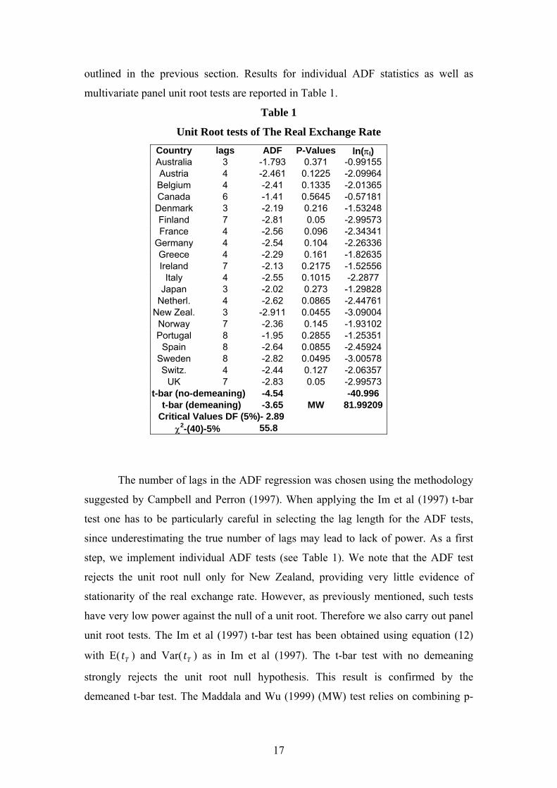
outlined in the previous section. Results for individual ADF statistics as well as

multivariate panel unit root tests are reported in Table 1.

Table 1

Unit Root tests of The Real Exchange Rate Country lags ADF P-Values ln(πI) Australia 3 -1.793 0.371 -0.99155Austria 4 -2.461 0.1225 -2.09964Belgium 4 -2.41 0.1335 -2.01365Canada 6 -1.41 0.5645 -0.57181Denmark 3 -2.19 0.216 -1.53248Finland 7 -2.81 0.05 -2.99573France 4 -2.56 0.096 -2.34341

Germany 4 -2.54 0.104 -2.26336Greece 4 -2.29 0.161 -1.82635Ireland 7 -2.13 0.2175 -1.52556

Italy 4 -2.55 0.1015 -2.2877 Japan 3 -2.02 0.273 -1.29828

Netherl. 4 -2.62 0.0865 -2.44761New Zeal. 3 -2.911 0.0455 -3.09004

Norway 7 -2.36 0.145 -1.93102Portugal 8 -1.95 0.2855 -1.25351

Spain 8 -2.64 0.0855 -2.45924Sweden 8 -2.82 0.0495 -3.00578Switz. 4 -2.44 0.127 -2.06357

UK 7 -2.83 0.05 -2.99573t-bar (no-demeaning) -4.54 -40.996

t-bar (demeaning) -3.65 MW 81.99209Critical Values DF (5%)- 2.89

χ2-(40)-5% 55.8

The number of lags in the ADF regression was chosen using the methodology

suggested by Campbell and Perron (1997). When applying the Im et al (1997) t-bar

test one has to be particularly careful in selecting the lag length for the ADF tests,

since underestimating the true number of lags may lead to lack of power. As a first

step, we implement individual ADF tests (see Table 1). We note that the ADF test

rejects the unit root null only for New Zealand, providing very little evidence of

stationarity of the real exchange rate. However, as previously mentioned, such tests

have very low power against the null of a unit root. Therefore we also carry out panel

unit root tests. The Im et al (1997) t-bar test has been obtained using equation (12)

with E( ) and Var( ) as in Im et al (1997). The t-bar test with no demeaning

strongly rejects the unit root null hypothesis. This result is confirmed by the

demeaned t-bar test. The Maddala and Wu (1999) (MW) test relies on combining p-

Tt Tt

17

values rather than t-statistics as the t-bar tests. P-values are obtained using the non-

parametric bootstrap procedure described in Cerrato and Sarantis (2004). The

Maddala and Wu (1999) also strongly rejects the unit root null. Overall, in line with

most empirical studies on PPP, such as Coakley and Fuertes (1997) and Wu (1996)

(Cerrato and Sarantis, 2004 being an exception14), panel unit root tests indicate that

the real exchange rate is stationary over the sample period and the panel of countries

we consider. 15

3. Panel Cointegration Tests and PPP 3.1 Panel Cointegration Tests Various researchers have used cointegration techniques to test PPP by estimating an

equation such as:

tttt upps +++= *

10 ββα (23)

or, when symmetry between domestic and foreign prices was imposed, an equation

such as:

)( *ttt pps −+= βα (24)

Early tests were based on the idea that PPP in its weak form implies that st, pt,

and *tp should be integrated of order one, I(1), and the residuals be stationary, I(0).

PPP in its strong form holds if the joint symmetry and proportionality restrictions are

also satisfied: 110 =−= ββ . Numerous empirical studies have been carried out. In

general, rejections of the null of cointegration are less frequent if CPI is used instead

of WPI, and more frequent if the US dollar rather than the German mark is chosen as

the numeraire currency. The Engle and Granger (1987) approach initially used is

known to have low power against the null hypothesis of non-cointegration (in addition

to restricting the cointegrating vector to be unique). The Johansen (1988) procedure,

14 However, Cerrato and Sarantis (2004) use monthly data while the majority of other studies, except Wu (1996), use quartely data. 15 Im et al (1997) also reject the null hypothesis, whilst Maddala and Wu (1999) do not.

18

which has higher power and allows for multiple cointegrating vectors, has

subsequently been employed. 16

Panel cointegration tests represented the next development. There are two

main approaches, one based on the null hypothesis of cointegration, as in McCoskey

and Kao (1998), the other on the null of no cointegration, as in Pedroni (1997, 1999).

The former propose a residual-based Lagrange Multiplier test to deal with the

nuisance parameters issue in a single equation model. The model is similar to those of

Pedroni (1997) and Im et al (1997). Assume that is generated as follows: ity

titiiiti exy ,

',, ++= βα (25)

where ∑ =

+=t

j tijiti uue1 ,,, θ

The model allows for different slopes and intercepts, and the residuals are

serially correlated. Furthermore, the regressors are assumed to be endogenous

and generated by

)( ',tix

tititi xx ,1,, ω+= − , but not cointegrated. Under the null hypothesis

H0:θ = 0, and the above equation is a system of cointegrated regressors.

McCoskey and Kao (1998) show that the test statistic is an LM statistic given by:

itit ue =

21 1

2

sS

LMN

i

T

t it∑ ∑= == (26)

where Si,t is the partial sum of the residuals, i.e , and s∑=

=t

jjiit eS

1

*,

2 is a consistent

estimator of σ2u.

If we allow for correlation in the error processes17, s2 can be estimated using

the dynamic OLS estimator (DOLS) or the fully modified OLS estimator (FMOLS)18.

16 Example of an empirical study using Johansen’s tests to test PPP is Enders and Falk (1998). 17 The serial correlation element could be particularly relevant in many empirical applications, including PPP. 18 As we shall see, in general the DOLS estimator performs better than the FMOLS estimator.

19

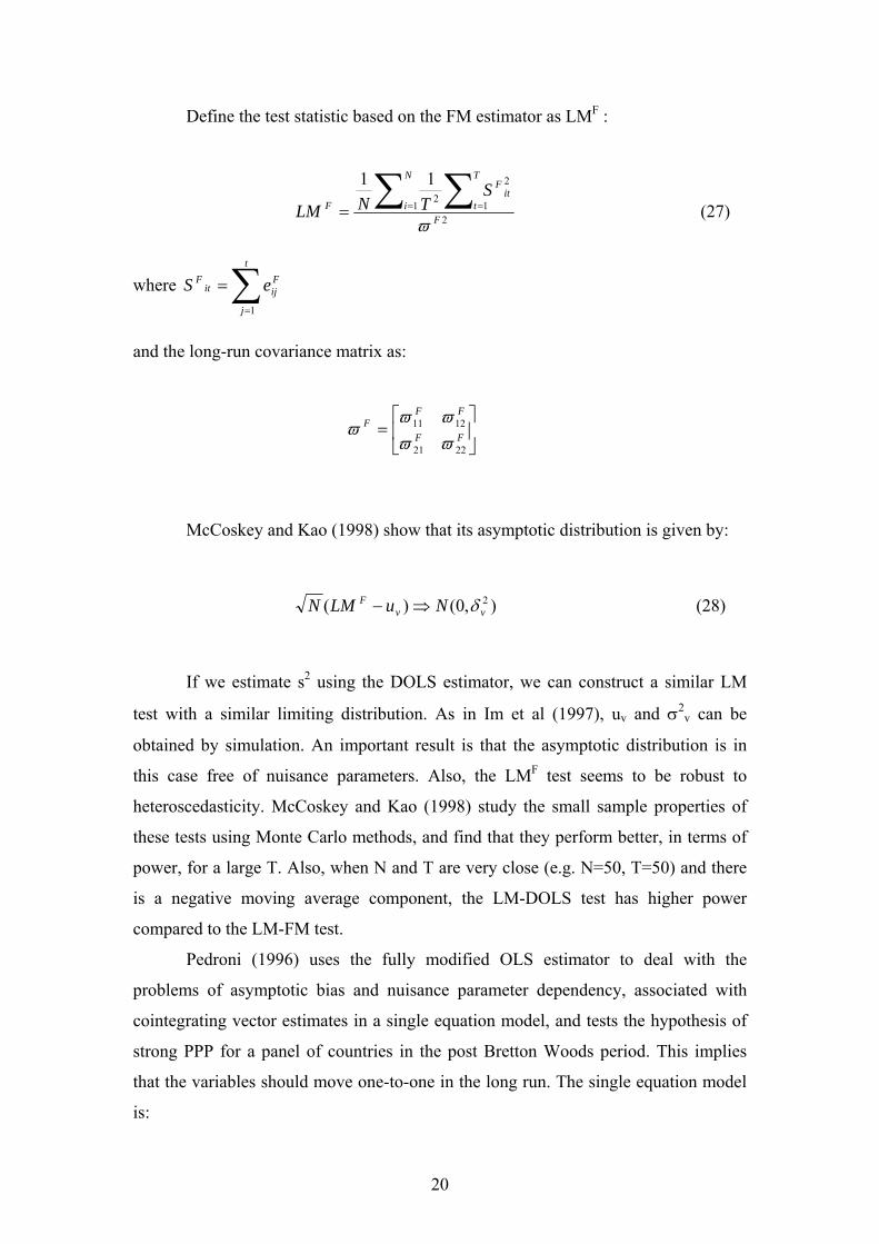
Define the test statistic based on the FM estimator as LMF :

21 1

2

2

11

F

N

i

T

tit

F

FS

TNLMϖ

∑ ∑= == (27)

where ∑=

=t

j

Fijit

F eS1

and the long-run covariance matrix as:

⎥⎦

⎤⎢⎣

⎡= FF

FFF

2221

1211

ϖϖϖϖ

ϖ

McCoskey and Kao (1998) show that its asymptotic distribution is given by:

),0()( 2vv

F NuLMN δ⇒− (28)

If we estimate s2 using the DOLS estimator, we can construct a similar LM

test with a similar limiting distribution. As in Im et al (1997), uv and σ2v can be

obtained by simulation. An important result is that the asymptotic distribution is in

this case free of nuisance parameters. Also, the LMF test seems to be robust to

heteroscedasticity. McCoskey and Kao (1998) study the small sample properties of

these tests using Monte Carlo methods, and find that they perform better, in terms of

power, for a large T. Also, when N and T are very close (e.g. N=50, T=50) and there

is a negative moving average component, the LM-DOLS test has higher power

compared to the LM-FM test.

Pedroni (1996) uses the fully modified OLS estimator to deal with the

problems of asymptotic bias and nuisance parameter dependency, associated with

cointegrating vector estimates in a single equation model, and tests the hypothesis of

strong PPP for a panel of countries in the post Bretton Woods period. This implies

that the variables should move one-to-one in the long run. The single equation model

is:

20

ititiit xy µβα ++= (29)

where yit is the log U.S. nominal exchange rate, and xit is the log aggregate price ratio

between the two countries in terms of the CPI, and strong PPP implies one-to-one

adjustment in the long run. 19

Pedroni (1997) proposes seven different panel cointegration tests. The

construction of such tests is complicated, because the residuals may depend on the

distribution of the estimated coefficients. He allows for considerable heterogeneity in

the panel. In fact, he assumes a heterogeneous slope coefficient, fixed effects and

individual specific deterministic trends. The model considered is a more general one

than the model given by (25):

titiiiiit exty ,,' +++= βδα t=1,2….T; i=1,…,N (30)

m=1,…M

where )',...,,( 211 Miii ββββ = , )',...,,( 21 Miitititi xxxx = , T refers to the number of

observations over time, N to the number of countries in the panel, and M to the

number of regressors.

An important assumption discussed by Pedroni (1997) concerns the cross-

member panel-wide properties of the data. Specifically, he assumes the idiosyncratic

error terms to be independent across individual members of the panel, and proposes a

GLS-based correction to allow for feedback across individual members of the panel.

Of his seven tests, four are based on a within-dimension approach, and three on a

between-dimension approach. In the first group we take the sum of both the

numerator and the denominator terms over the N dimension. In the second group, we

divide the numerator by the denominator prior to summing over the N dimension. We

shall describe the construction of the seventh test, which is a parametric one.

19 Pedroni (1996) tests the null hypothesis H0: βi=1 and finds evidence supporting weak but not strong PPP. One of the most recent papers using cointegration methods to test PPP is due to Canzoneri et al. (1999). They use traded goods prices, the German mark as the numeraire currency and the panel cointegration test proposed by Pedroni (1996), finding support for long-run PPP.

21

1) Estimate the panel cointegration regression (30) and retrieve the residuals *,tie

2) Run the panel regression in first differences: t=1,2…,T;

i= 1,..N and compute the residuals.

titiiti xy ,,'

, ηβ +∆=∆

3) Calculate the long-run variance of η*, ¦*21

1*22

*21

*11

2*11 iiiiiL ΩΩΩ−Ω= −

4) Using the residuals e*it, estimate ∑ = −− +∆+=Ki

K tiktikitiiti eee1

*,

*,

*,

*1,

**, µγγ and

use the residuals to compute the sample variance of denoted by . *itµ 2*

is

The panel t-statistic is then defined as follows:

∑ ∑ ∑= = =

−−

−−− ∆=

N

i

T

t

T

ttititiiTtN eeesNZN

1 1 1

*,

*1,

2/12*1,

2*2/1*,

2/1 )( (31)

This statistic can be viewed as analogous to the LL panel unit root test statistic

applied to the estimated residuals of a cointegration regression. Let be

such that the process z

)',( ititit xyz =

it is generated by zit=zi,t-1+ςit, for . Assume that

the process can be characterised in terms of standard Brownian

motion. In this case, all we need to determine the complete distribution of the process

above is its covariance structure Ω

)',( xit

yitit ςςς =

)',( xit

yitit ςςς =

i (i.e., only the first two moments of the process).

Also, assume that the error terms are independent across individual members of the

panel. Under these two assumptions, the central limit theorem holds for each

individual series as T grows large. The statistic described above can subsequently be

standardised, relying on the moments of the Brownian motion function. If we denote

with Θ* and Ψ* the vector of means and the covariance matrix, its asymptotic

distribution is given by N-1/2z*t,N,T-Θ*2 ⇒N N(0,Ψ*22). This is an important result,

as it tells us that the standardised statistic converges to a normal distribution whose

moments depend on Ψ* and Θ*.

These moments20 can be obtained by Monte Carlo simulation and used to re-

write the asymptotic distribution as follows:

20 Note that, although the statistics, under appropriate standardisation, converge to a normal distribution, there is no formal proof that the moments of the distribution are finite for each N,T. This technical difficulty also arises in the case of the t-bar test.

22

)1,0(, Nv

Nuk TN ⇒−

(32)

where is the panel cointegration statistic, and u and ν are functions of the

moments of the Brownian function.

TNk ,

Pedroni (1997) performs Monte Carlo simulations to study the small sample

(power and size) properties of these seven statistics. He finds that the size distortions

for all the proposed panel cointegration statistics are small, provided that there is not a

negative moving average component in the DGP. Also, size distortions are small for

T=250 and larger for a smaller T. Further, the power of the panel cointegration

statistics is very high when T=100 and T=250. In brief, in terms of size distortion, the

panel-rho statistic seems to exhibit the least distortions among the seven statistics.

The group ADF exhibits the largest size distortions. In terms of power, the group

ADF does very well, followed by the panel ADF and the panel-rho21.

All the panel cointegration tests presented above are residual-based, and do

not allow for the possibility of multiple cointegrating vectors. Larsson et al (2001)

address this issue, and propose a likelihood-based test of the cointegrating rank in

heterogeneous panels. Assume that the data generating process for each of the groups

is represented by the following VAR (ki)22:

∑=

− +Π=ik

k

itktiikit yy1

, ε i=1,…,N (33)

As shown by Engle and Granger (1987), the corresponding error correction

representation is the following:

∑=

−− +∆Γ+Π=∆ki

kitktiiktiiit yyy

1,1, ε i=1,…N (34)

21 Cerrato and Sarantis (2002) use the seven panel cointegration tests suggested by Pedroni (1997) to test for cointegration in a trivariate PPP framework using monthly nominal exchange rates and a panel of twenty OECD countries. After testing for the validity of the joint symmetry and proportionality restrictions, they conclude that unit root tests of the real exchange rate may be biased towards finding no evidence of PPP. Panel tests, though more supportive of PPP, still produce mixed results. 22 In what follows, one may think of as being the real exchange rate. ity

23

where Πi is of order pp× ( p being the number of variables in each group). The

matrix Πi can be decomposed into Πi = 'iiβα , where αi and βi are matrices of order p×

ri representing the long-run coefficients and the adjustment parameters respectively.

Consider the following null and alternative hypotheses:

H(r): rank (Π) ≤ r

H(p) : rank (Π) = p

As in Johansen (1988), the likelihood ratio test (the trace statistic) 23 can then

be written as follows:

∑+=

−=−−p

riTi pHrHQT

1

* ))(¦)((ln2)1ln( λ (35)

Since we are interested in testing the hypothesis that all N groups in the panel

have the same number of cointegrating relationship (r=ri), the null and the alternative

can be specified as:

H0: rank(Πi)=ri ≤ r for all i=1…N

H(p) : rank (Πi) = p for all i=1…N

The LR-bar statistic can be defined as the average of the N individual trace

statistics LRiT (H(r) ¦ H((p)): 24

))(¦)((/1))(¦)((1

pHrHLRNpHrHLRN

i

iTNT ∑=

= (36)

Using a standardisation procedure, one obtains the standardised LR–bar

statistic for panel cointegration:

23 Note that the trace statistic refers to each group i.

24

)())())(¦)(((

))(¦)((k

KNTbarLR ZVar

ZEpHrHLRNpHrH

−=−γ (37)

where E(ZK) and Var (ZK) are the mean and variance of the asymptotic trace statistic.

The original contribution made by Larsson et al (2001) is to show that every

study performed in a non-panel context can be extended to a panel framework.

Furthermore, by proposing the panel data analogue of the Johansen maximum

likelihood method, they are able to study the case of multiple cointegrating vectors in

panels 25.

In Larsson et al (2001) a common cointegrating rank is simply assumed.

Larsson and Lyhagen (2000) suggest the following way to test this hypothesis. First,

the LR-bar statistic of Larsson et al (2001) is applied to obtain the maximum rank

amongst the N individual ones. Then, a panel test (PC-bar) is implemented to test the

hypothesis of r cointegrating vectors against r-1. This is based on the test proposed by

Harris (1997). If the two tests coincide, the null of the same number of cointegrating

relations cannot be rejected, otherwise the null hypothesis is rejected and the

alternative is accepted.

Larsson and Lyhagen (1999) derive two test statistics in the context of a panel-

VAR with cointegrating restrictions: a likelihood ratio test for the cointegrating rank,

and another for a common cointegrating space. Let i=1,…N be the index for the

groups, t=1,…T the sample time period and j=1,…p the variables in each group, with

yijt denoting the ith group, jth variable at time t. Consider the following model:

∑−

=−− +∆Γ+=∆

1

11

m

ktktktt yyy ςπ (38)

where yt = ( yξ1t, yξ2t, …yξNt)ξ is the Nxp vector of the panel of observations available

at time t on the p variables for the N groups, and ς = (ςξ1t,…ςξNt)ξ with ς∼N (0, Ω). π

and Γ can be divided into submatrices πij and Γij i,j=1,…N.

24 This test is based on the approach suggested by Im et al (1997) for the univariate unit root panel test statistic. 25 Cerrato and Sarantis (2002) apply the Larsson et al (2001) tests in a trivariate PPP framework using a panel of twenty monthly nominal exchange rates, and report strong evidence of cointegration.

25

Since the rank of π is Σri, where 0≤ri≤p, we can write π as π= ABξ, where A

and B are two matrices of order Np× Σri, with A containing the short-run coefficients

αij and B the long-run coefficients βij, each being of rank ri. At this point an important

restriction is discussed by Larsson and Lyhagen (1999). They assume that βij =0 but

αij≠ 0. In this way, the model allows short-run, but not long-run dependence between

the panel groups. The off-diagonal elements in 'AB=π , that is 'jijij βαπ = , represent

the short-run dependencies of the changes in the series for group i due to long-run

equilibrium deviations in group j. These assumptions enable Larsson and Lyhagen

(1999) to re-write the model (38) in the following form:

∑−

=

−− +∆Γ+=∆1

1

1'm

k

tktktt yyABy ς (39)

Given the model and two homogeneity restrictions, B=Diag(βii) and B= (IN ⊗ β),

model B= (IN ⊗ β) is tested against B=Diag(βii). The distribution of the test for the

cointegrating rank and for a common cointegrating space are shown respectively to be

equal to the convolution of a Dickey-Fuller type distribution and an independent χ2

variate, and a χ2 distribution, with the number of degree of freedom given by (N-

1)r(p-r).

3.2 An Empirical Example

In this subsection we apply some of the panel cointegration tests described above; in

particular, we focus on heterogeneous panel cointegration, that is, the seven panel

tests proposed by Pedroni (1997) and the Larsson et al (2001) test. We use a trivariate

PPP framework without imposing any a-priori symmetry restriction. The results of the

Pedroni test are reported in Table 2:

26

Table 2

Pedroni (1997) Panel Cointegration tests Panel v-Statistic 2.12611Panel rho-statistic 0.48956Panel pp-statistic 0.34276Panel ADF-statistic 0.83774Group Rho-statistic 1.6804Group pp-statistic 1.68045Group ADF-statistic 2.2638

The Pedroni (1997) panel cointegration tests cannot reject the null hypothesis of no

cointegration, with the exception of the panel v-statistic, implying little evidence in

favour of PPP. Note that the Pedroni (1997) statistics have critical values of -1.64

( suggests a rejection of the null). The 64.1<k ν statistic has a critical value of 1.64

( suggesting a rejection of the null). Means and variances used to calculate

these statistics are from Pedroni (1999, Table 2), with heterogeneous intercepts

included. The results for the Larsson et al (2001) test are reported in Table 3. This test

relies on combining N-trace statistics.

64.1>k

Table 3

Larsson et al (2001) Panel Cointegration Test Lags r = 0 r = 1 r = 2 Max Rank

Australia 1 15.144 15.144 0.258 1 Austria 6 42.346 17.668 1.965 2 Belgium 5 72.11 31.12 0.017 3 Canada 1 24.86 7.51 0.827 0 Denmark 6 31.18 14.71 1.448 1 Finland 2 35.69 10.42 2.802 1 France 8 35.53 8.98 0.028 1 Germany 2 31.84 5.75 1.88 1 Greece 3 46.82 16.4 3.89 3 Ireland 2 38.46 15.68 1.76 2 Italy 8 22.6 7.58 0.83 0 Japan 5 38.15 19.11 0.011 3 Netherl. 1 54.36 12.68 2.56 1 New Zeal. 4 23.82 11.10 0.002 0 Norway 7 36.5 14.9 4.65 1 Portugal 5 36.89 15.58 3.37 2 Spain 4 37.69 19.11 4.2 3 Sweden 2 34.27 14.12 0.003 1 Switz. 2 41.58 10.77 2.088 1 UK 1 50.86 14.33 0.004 1 Average 37.53 14.13 1.6296 Test 20.3 11.08 1.48 Johansen CV- (5%) r = 0, 29.68 r=1, 15.41 r=2, 3.76

27

The individual trace statistics indicate that for most of the countries in our panel the

maximum rank is 1. In the case of Spain, Japan, Greece and Belgium it is found to be

three. The trace test implies no cointegration in only three cases, i.e. Canada, Italy and

New Zealand. The Larsson et al (2001) test statistic is reported at the bottom of the

table. It has been computed using equation (37) with mean and variance obtained

from Larsson et al (2001). Since the test follows a normal distribution its 5% critical

value is 1.645. It suggests that there exist two cointegrating vectors between the

nominal exchange rate, domestic prices and foreign prices.

This example illustrates clearly that, when carrying out panel cointegration

tests of PPP, one should (a) allow for heterogeneity when testing for cointegration

between the nominal exchange rate, domestic and foreign prices, and (b) avoid a-

priori restrictions such as symmetry restriction.

4. Some Unresolved Issues in Panel Unit Root and Cointegration Tests

Despite the considerable progress made in the area of panel data econometrics,

several unresolved problems remain. For instance, there is extensive Monte Carlo

evidence indicating size distortions and low power in the commonly used unit root

tests26. The empirical distribution of these tests is very different from the asymptotic

one in the presence of negative moving average errors. In this case, the

implementation of unit root tests often necessitates a large autoregressive truncation

lag (k). Monte Carlo simulations have demonstrated an association between k and the

severity of size distortion27 (Ng and Perron, 1999). If the moving average components

are small, a small k is adequate. On the other hand, if they are large, a large value of k

is required. However, such a strategy may not be feasible, since selecting a large k

may lead to overparameterisation and a consequent loss of power. The difficulty with

the most common methods for selecting a value of k, i.e. the Akaike Information

Criterion (AIC) and the Schwarz Information Criterion (SIC), is that they tend to

select a value of k which is too small. The bias in the estimated sum of the

26 The two problems should be kept distinct (see Ng and Perron, 1999). Low power arises when the dominant root is near, but not exactly equal to, unity. Size distortion may arise, for example, when the underlying distribution contains a negative moving average component. However, in panel data, size distortion may also arise from cross-sectional dependence. 27 Simulations for T=100 and 250 have provided evidence that the size issue in the negative moving average case is not a small sample problem. In this case, the consequence is over-rejection of the unit root hypothesis (Ng and Perron, 1999).

28

autoregressive coefficients (β*0) might depend on k in the presence of a negative

moving average component. To see the problem, assume the following data

generating process (DGP):

(40) ttt udy += dt=ϕ¦zt

where zt is a set of deterministic components ttt uu να += −1 1−+= ttt eev φ (41) The Dickey-Fuller test (1979) is the t-statistic for β0 in the autoregression:

(42) ∑=

−− +∆++=∆k

jtkjtjttt uyydy

110 ββ

The AIC or the SIC methods for selecting k belong to the class of information-

based criteria (IC) where the value of k is kic = arg. mink IC (k):

IC(k)= log (δk*2)+(k)Ct/T (43)

with , C∑+=

−=T

kttkk uT

1

*212*δ t/T→0 as T→∞ and Ct>0, where Ct is the weight applied to

overfitting.

We select k* such that limt→∞ E(T(k-k*))=0, i.e. to minimise the objective

function (43) (see Gourieroux and Monfort, 1995). However, this method does not

allow for the possibility that the bias in the estimated sum of the autoregressive

coefficients:

∑+=

−−=

T

kttkT yk

1

2*1

2*0

12* )()( βδπ (44)

29

might depend on k in the presence of a negative moving average component. The

reason is that this bias is very high for small values of k, and, unless k is very large, it

persists and becomes highly dependent on k.28 Based on this evidence, Ng and Perron

(2001) show that the modified Akaike information criterion (MAIC) gives the best

combination of size and power29.

Another very important issue in panel unit root and cointegration tests is the

structure of the covariance matrix, which is generally assumed to be diagonal. As

pointed out by Im et al (1997), this requires the observations to be generated

independently across different groups, that is, no cross-sectional dependence. There

are currently two strands of the literature dealing with a non-diagonal covariance

matrix. The first has focused mainly on the correlation between group of observations

(i.e. cross-sectional dependence), the second on group dependence in the innovations.

As we shall stress below, in general the two are closely related.

Panel data refers to the pooling of observations on a cross-section of

households, countries, firms, over several time periods. This can be achieved by

surveying a number of households or individuals and following them over time. We

obtain a combination of time series and cross-section data. But why should one be

concerned with cross-sectional dependence? Recall that the properties of all the tests

described before are based on the assumption that data in one group are generated

independently from those in another group - in other words, that there is no

dependence between different groups of observations. Provided that this assumption

holds, one can use the central limit theorem and derive the asymptotic distribution for

28 Different methods have been suggested to deal with this problem. For example, Carner and Kilian (1999) report extreme size distortions for the Leybourne and McCabe (1994) test and the KPSS test. They consider a highly persistent model under the null of stationarity, and a unit root process under the alternative. They overcome the size distortions using appropriately adjusted finite sample critical values, and demonstrate that such corrections inevitably result in a dramatic loss of power in the tests. However, these results should be interpreted with caution, as the DGP assumed is an AR(1) process with root ρ and NID (0,1) innovations. Furthermore, the number of lagged terms (l) is selected using a procedure for a fixed l as a function of T, i.e. l= int (C(T/100)1/d) with c=12 and d=4 , which might lead to overparameterisation and loss of power. Furthermore, the finite sample critical values are derived from a parametric model, which clearly violates the nonparametric spirit of the KPSS test. 29 Recently Lopez et al (2002) report evidence suggesting that the MAIC criterion works well with DF-GLS tests, but for ADF tests the Campbell and Perron (1997) method is preferable.

30

a particular panel estimator30. There are different kinds of cross-sectional correlation:

homogeneous, quasi heterogeneous and heterogeneous. Consider, for instance, the

relationship between the Swiss and UK real exchange rates, where the US dollar is

used as the numeraire currency. The two will be correlated, as by construction they

contain two common elements, i.e. the independent variation in the value of the dollar

and in the US price index (O` Connell, 1998). Consider the following real exchange

rate model:

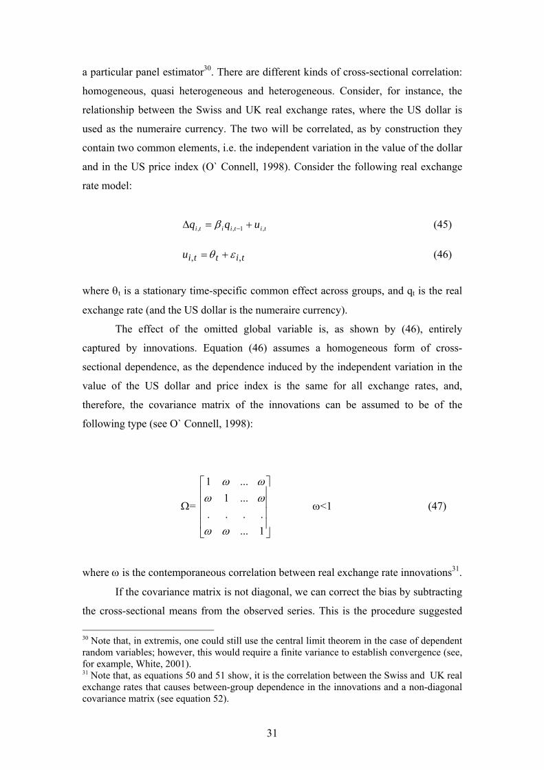
titiiti uqq ,1,, +=∆ −β (45) tittiu ,, εθ += (46)

where θt is a stationary time-specific common effect across groups, and qt is the real

exchange rate (and the US dollar is the numeraire currency).

The effect of the omitted global variable is, as shown by (46), entirely

captured by innovations. Equation (46) assumes a homogeneous form of cross-

sectional dependence, as the dependence induced by the independent variation in the

value of the US dollar and price index is the same for all exchange rates, and,

therefore, the covariance matrix of the innovations can be assumed to be of the

following type (see O` Connell, 1998):

Ω= ω<1 (47)

⎥⎥⎥⎥

⎦

⎤

⎢⎢⎢⎢

⎣

⎡

1.......

...1

...1

ωω

ωωωω

where ω is the contemporaneous correlation between real exchange rate innovations31.

If the covariance matrix is not diagonal, we can correct the bias by subtracting

the cross-sectional means from the observed series. This is the procedure suggested

30 Note that, in extremis, one could still use the central limit theorem in the case of dependent random variables; however, this would require a finite variance to establish convergence (see, for example, White, 2001). 31 Note that, as equations 50 and 51 show, it is the correlation between the Swiss and UK real exchange rates that causes between-group dependence in the innovations and a non-diagonal covariance matrix (see equation 52).

31

by Im et al (1997), 32 which can be summarised in the following way. Consider the

following DGP for the real exchange rate : itq

tiititi uqq ,1, += −β Ni ,...,1= Tt ,...,1= (48)

Equation (48) consists of i countries observed t times. It is convenient for our

purposes to stack (48) into N equations as follows:

ttt uqq += −1β (49)

with each of the N equations consisting of T observations.

Define by a vector that contains columns of ones. Then

. Also, define the covariance matrix as . Finally, consider two

different cases for Ω . In the first the covariance matrix is assumed to be diagonal,

whilst in the second it takes the form given in (47). By using the demeaning procedure

the covariance matrix reduces to:

]1,...,1['=i

NNii ×=' )( 'ttuuE=Ω

'))(( AV

ttAVtt uuuu −−=Ω where is the average of (50) AV

tu tu

Define the following idempotent symmetric matrix '1 iiN

IP −= and

]1,..,1['=i

⎟⎟⎟⎟⎟⎟⎟⎟⎟

⎠

⎞

⎜⎜⎜⎜⎜⎜⎜⎜⎜

⎝

⎛

−

−−

−−−

−−−−

=×

N

NN

NNN

NNNN

P NN

11

111

1111

1.1111

(51)

32 Under these assumptions, and if cross-sectional dependence is of a weak-memory variety, the central limit theorem may still apply. However, when there are strong correlations in a cross-section (as there will be in the presence of global shocks), we may expect it to fail (see Phillips and Moon, 1999).

32

Using the general expression of the covariance given above and (51), we obtain:

*')( Ω=tt PuPu

''* PuPu tt=Ω

'* PPΩ=Ω (52)

Equation (52) represents the covariance matrix after the demeaning procedure.

It is straightforward to see that it is no longer diagonal. This result is not surprising

since it is the subtracting of the cross-sectional means that determines cross-sectional

dependence: we are subtracting a common element (same information) from each

cross-unit33.

Let us consider the case when the covariance matrix is not diagonal and of the

form given in (47)34. By using (47) in conjunction with (51) we have:

')1( iiI ωω +−=Ω

PiiIiiN

IPP ])1)[(1( ''' ωω +−−=Ω (53)

which after some algebra reduces to: (54) PPP )1(' ω−=Ω

It is clear from (54) that, in the presence of cross-sectional dependence, the

covariance matrix depends on the parameter ω that measures its degree. The

33 By doing so, we may lose important information. One solution is to model the cause of dependence between groups of innovations. 34 Note that we are considering only a limited case of cross-sectional dependence, i.e. of a homogeneous type. Modelling the covariance matrix in the case of heterogeneity is much more complicated.

33

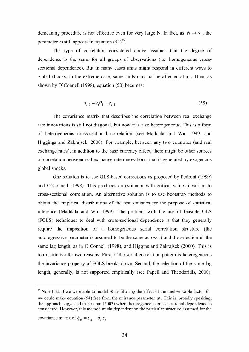
demeaning procedure is not effective even for very large N. In fact, as , the

parameter

∞→N

ω still appears in equation (54)35.

The type of correlation considered above assumes that the degree of

dependence is the same for all groups of observations (i.e. homogeneous cross-

sectional dependence). But in many cases units might respond in different ways to

global shocks. In the extreme case, some units may not be affected at all. Then, as

shown by O`Connell (1998), equation (50) becomes:

tititi ru ,, εθ += (55)

The covariance matrix that describes the correlation between real exchange

rate innovations is still not diagonal, but now it is also heterogeneous. This is a form

of heterogeneous cross-sectional correlation (see Maddala and Wu, 1999, and

Higgings and Zakrajsek, 2000). For example, between any two countries (and real

exchange rates), in addition to the base currency effect, there might be other sources

of correlation between real exchange rate innovations, that is generated by exogenous

global shocks.

One solution is to use GLS-based corrections as proposed by Pedroni (1999)

and O`Connell (1998). This produces an estimator with critical values invariant to

cross-sectional correlation. An alternative solution is to use bootstrap methods to

obtain the empirical distributions of the test statistics for the purpose of statistical

inference (Maddala and Wu, 1999). The problem with the use of feasible GLS

(FGLS) techniques to deal with cross-sectional dependence is that they generally

require the imposition of a homogeneous serial correlation structure (the

autoregressive parameter is assumed to be the same across i) and the selection of the

same lag length, as in O`Connell (1998), and Higgins and Zakrajsek (2000). This is

too restrictive for two reasons. First, if the serial correlation pattern is heterogeneous

the invariance property of FGLS breaks down. Second, the selection of the same lag

length, generally, is not supported empirically (see Papell and Theodoridis, 2000).

35 Note that, if we were able to model ω by filtering the effect of the unobservable factor tθ , we could make equation (54) free from the nuisance parameter ω . This is, broadly speaking, the approach suggested in Pesaran (2003) where heterogeneous cross-sectional dependence is considered. However, this method might dependent on the particular structure assumed for the

covariance matrix of −

−= tiitit εδεξ

34

Furthermore, the consistence of the FGLS estimator relies on that of the estimator

used to estimate the covariance matrix. Usually, the latter is the Pooled Least Square

Estimator (POLS). Coakley et al (2002) show that, under cross-sectional dependence,

this estimator is inconsistent36.

Another strand of literature has preferred to focus on between-group

correlation of innovations. In fact, we could have a situation where a non-diagonal

covariance matrix arises from the omission of a variable that is completely

uncorrelated with the included regressors. In other words, there might be no

correlations between different groups of observations, but because the effect of the

omitted variable is captured by the innovations, the covariance matrix will not be

diagonal. SURE procedures have been recommended in this case. The logic behind

such an approach is that, since the efficiency of the SURE estimator increases with

the degree of correlation between the innovations, relative to correlation between

groups of observations, one should gain in efficiency by using it. However, since the

SURE approach in panels consists in a multivariate FGLS procedure, all the

drawbacks highlighted above are also relevant here. Furthermore, if the cause of a

non-zero diagonal covariance matrix is the omission of a global variable that is

correlated with the included regressors (that is, if we have cross- sectional

dependence), then the SURE estimator is not necessarily superior to the OLS

estimator (see Maddala, 2002).

Recently, Banerjee et al (2001) noted another source of size distortion in panel

unit root and cointegration tests in addition to cross-sectional dependence, namely the

presence of cointegration between different groups. 37 They perform Monte Carlo

simulations showing that this is the case for some of the most common panel unit root

and cointegration tests (i.e. LL, 1993, Im et al, 1997 and Maddala and Wu, 1999) 38.

The panel unit root test that suffers the least from size distortion is the LL2 (1993)

one. The implication for applied work is the same as in the presence of cross-

36 Phillips and Soul (2003) also show that, under cross-sectional dependence, both the POLS and the FGLS estimators are biased. However, we can always estimate the covariance matrix by using a non-parametric approach. 37 Cross-cointegration can be viewed as long-run cross-correlation between different groups. It could be due, for example, to a common stochastic trend driving different groups, and as such it has been analysed by Bai and Ng (2002a), and Larsson and Lyhagen (2000). 38 Lyhagen (2000) also studies the size of different panel unit root and cointegration tests in the presence of cointegration across units. He finds the McCoskey and Kao (1998) test to perform better than the Im et al (1997) under these circumstances.

35

sectional dependence, that is, the null hypothesis is rejected too often. However, the

Monte Carlo experiments conducted by Banerjee et al (2001) might be biased in

favour of the LL test. In fact, their Monte Carlo experiments are entirely calibrated on

the LL test39. Consequently, it is not surprising that the LL test should be found to

perform better than the others in the presence of cointegration between groups: this

result might simply reflect the Monte Carlo design. Furthermore, they compare tests

based on different hypotheses. Recall that the Im et al (1997) test is a heterogeneous

test where the alternative is that some units are stationary while some others are not.

On the other hand, the LL is a homogeneous test with the alternative that all units are

stationary. This comparison between tests testing different hypotheses might not be

entirely appropriate after-all.

5. Conclusions

This paper provides a critical overview of the major panel unit root/cointegration tests

used in the literature to test long-run PPP. We have outlined the unit root tests

introduced by Levin and Lin (1993), Im et al (1997), Taylor and Sarno (1998) and

Maddala and Wu (1999) and highlighted their limitations. We have also discussed

some panel cointegration tests such as the ones proposed by Larsson et al (2001),

Pedroni (1997) and McCoskey and Kao (1998). We have considered (i) the role of

ADF regressions as a way of allowing for serially dependent and heteroscedastic

residual processes; (ii) the problem of heterogeneity in panel unit root and

cointegration tests and its implication for applied work on PPP; (iii) the problem of

endogeneity in cointegration tests; (iv) the low power and size distortion of unit root

tests in the presence of a negative moving average component. An important common

feature of all of the tests presented in this survey is that their asymptotic distributions

were derived under the assumption of no correlation between groups of observations,

which implies a diagonal covariance matrix. We have pointed out that this assumption

is often violated, and therefore the asymptotic distributions of panel estimators may

no longer be reliable. Different approaches have been suggested in the literature to

deal with cross-sectional dependence and a non-diagonal covariance matrix.

However, further investigation is still required.

39 They adopt exactly the same Monte Carlo design as in Levin and Lin, 1993.

36

The main lessons to be learned from this overview can be summarised as

follows. First, size distortion in panel unit root tests increases the likelihood of type-I

errors. Panel tests that assume i.i.d. disturbances suffer from severe size biases, that is,

the derived distributions are not valid and should not be used to draw statistical

inference. FGLS or SURE techniques are unlikely to provide a solution to the

problem. The assumption of a homogeneous slope parameter is too restrictive in many

applied contexts, and in particular for testing PPP.

Researchers have used panel unit root tests to overcome the problem of the

low power of the univariate unit root tests implemented in the early literature on PPP,

and found stronger evidence supporting PPP, especially for German mark-based

bilateral exchange rates, though the empirical findings are still mixed, and the issue of

whether or not long-run PPP holds is yet to be settled conclusively. Very little work

has been done using panel cointegration tests. Therefore, a final and relevant question

to be asked is: are panel methods likely ever to solve the PPP puzzle? We believe that

they might not provide the solution that was being sought by researchers. It is well

known that most time series estimators (for instance, OLS) suffer from small sample

bias. This is a serious problem in time series analysis, especially when estimating

half-lives deviations of the real exchange rate from PPP (see Murray and Papell,

2002). Phillips and Soul (2003) show that in panels small sample bias and cross-

sectional dependence work jointly, that is one reinforces the other, in this way making

inference in panels almost impossible. In other words, most of the typical problems

we encounter in time series analysis are amplified in panel analysis, with the

implication that it is even more difficult to obtain clear-cut results.

A more promising direction for future research on PPP might be to use non-

linear estimators. The importance of non-linearities in exchange rate modelling has

become increasingly clear in recent years (see Taylor and Peel, 2000). Estimating

non-linear models might at last provide more conclusive evidence, and explain the

PPP puzzle without the need to wait for a much larger number of observations to

become available, as required for standard linear estimators to have sufficiently high

power.

37

References

Bai, J., and Ng, S., 2002a, “Determining the Number of Factors in Approximate Factor Models”, Econometrica, 70, 191-221.

Bai, J., and Ng, S., 2002b, “A Panic Attack on Unit Roots and Cointegration”, Department of Economics, Boston College, Unpublished Manuscript.

Banerjee, A., 1999, “Panel Data Unit Roots and Cointegration: An Overview”, Oxford Bulletin of Economics and Statistics, 61, 607-629.

Banerjee, A., M. Marcellino and C. Osbat, 2001, “Testing PPP: Should We Use Panel Methods?” European University Institute, Working Papers.

Campbell, J. Y, and P., Perron, 1991, “ Pitfalls and Opportunities: What Macroeconomists Should Know About Unit Roots” NBER, Macroeconomics Annals, Vol. 6, O.J. Blanchard and S. Fisher (eds.).

Carner, M. and Kilian, L., 1999, “Size Distortions of Tests of the Null Hypothesis of Stationary: Evidence and Implications for the PPP Debate”. University of Michigan, Working Papers in Economics.

Canzoneri, B., M., Cumby, R., and B., Diba., 1999, “Relative Labour Productivity and the Real Exchange Rate in the Long-Run: Evidence for a Panel of OECD Countries”. Journal of International Economics, 47, 245-266.

Cassell, G., 1918, “Abnormal Deviations in International Exchanges”, Economic Journal, 413-415.

Cerrato, M., and N., Sarantis 2002, “Panel Cointegration Tests of Purchasing Power Parity”, D.P. no. 02-4, Centre for International Capital Markets, London Metropolitan University.

Cerrato, M., and N., Sarantis, 2004, “Cross Sectional Dependence, Panel Unit Root Tests, and Purchasing Power Parity”, D.P. no. 04-2, Centre for International Capital Markets, London Metropolitan University.

Coakley, J. and Fuertes, A.M., 1997, “A New Panel Unit Root Test of PPP” Economic Letters, 57, 17-22.

Coakley, J., and Fuertes, A.M, 2000, “Is There a Base Currency Effect in Long Run PPP?", International Journal of Finance and Economics, 5, 4, 253-263.

Coakley, J., A.,Fuertes and R., Smith, 2002, “A Principal Components Approach to Cross section Dependence in Panels”. Birkbeck College, Economics Working Papers.

Dickey, D.A., and Wayne A., Fuller, 1979, “Distribution of the Estimators for Autoregressive Time Series with a Unit Root”, Journal of the American Statistical Association, 74, 427-431.

Dickey, D.A., and Wayne A., Fuller, 1981, “Likelihood Ratio Statistics for Autoregressive Time Series with a Unit Root”, Econometrica, 49, 1057-1072.

Enders, W., and Falk, B., 1998, “Threshold-Autoregressive, Median Unbiased, and Cointegration Tests of Purchasing Power Parity”. International Journal of Forecasting, 14, 171-186.

Engle, R.F and C.W.J. Granger, 1987, “Co-integration and Error Correction: Representation, Estimation and Testing”, Econometrica, 55, 251-276.

Fisher, R.A, 1932, Statistical Methods for Research Workers, 4th ed, Oliver and Boyd, Edinburgh.

Frankel, J, A. and Rose, A., K., 1996, “A Panel Project on Purchasing Power Parity Within and Between Countries”, Journal of International Economics, 40, 209-224.

38

Froot, K., A., and Rogoff, K., 1995, “Perspectives on PPP and Long-Run Real Exchange Rates, in Rogoff, K., and Grossman, G., (eds), Handbook of International Economics, Amsterdam: North Holland.

Gourieroux, C. and Monfort, A. 1995, Statistical and Econometric Models, Vol. 1, Cambridge University Press, Cambridge.

Hall, S.G. and G. Urga, 2000, “New Developments in the Analysis of Panel Data Sets”, in S.B. Dahiya (ed.) The Current State of Business Disciplines, Vol.2 (Business Economics), Chapter 28, pp.537-564.

Harris, D., 1997, “Principal Component Analysis of Cointegrated Time Series”, Econometric Theory, 13, 529-557

Harris, D., and E., Tzavalis, 1999, “Inference for Unit Roots in Dynamic Panels where the Time Dimension is Fixed”, Journal of Econometrics, 91, 201-226

Higgins, M. Zakrajsek, E., 2000, “Purchasing Power Parity: Three Stakes Through the Heart of the Unit Root Null”, Federal Reserve Bank of New York, Working Papers.

Im, K-S., Pesaran M.H and Shin Y., 1997, “ Testing for Unit Roots in Heterogeneous Panels”, WP 9526, DAE, University of Cambridge. Revised June 1997.

Johansen, S., 1988, “Statistical Analysis of Cointegration Vectors”, Journal of Economic Dynamics and Control, 12, 231-254.

Karlsson, S., and M., Lothgren, 2000, “On the Power and Interpretation of Panel Unit Root tests”, Economics Letters, 66, 249-255.

Koedijk, G., K et. al , 1998, “ The Re-emergence of PPP in the 1990s”, Journal of International Money and Finance, 17, 51-61.

Koedijk, G., K., Schotman, P., C., 1990 “How to Beat the Random Walk: An Empirical Model of Real Exchange Rates”. Journal of International Economics 29, 311-332.

Kwiatkowski, D., P.C.B. Phillips, P. Schmidt, and Y. Shin, 1992, “ Testing the Null Hypothesis of Stationarity against the Alternative of a Unit Root”. Journal of Econometrics, 54, 159-178.

Larsson, J., Lyhagen and M., Lothgran, 2001, “Likelihood-Based Cointegration Tests in Heterogeneous Panels”, Econometrics Journal, 4, 109-141.

Larsson, R and J., Lyhagen, 1999 “ Likelihood Based Inference in Multivariate Panel cointegration Models”, Working Papers Series in Economics and Finance No. 331, Stockholm School of Economics.

Larsson, R and J., Lyhagen, 2000, “ Testing for Common Cointegrating Rank in Dynamic Panel”, Working Papers Series in Economics and Finance No. 378, April 21, Stockholm School of Economics.

Leybourne, S. and McCabe, B. (1994). "A consistent test for a unit root," Journal of Business and Economic Statistics, 12, 157-186.

Levin, A, and Lin, C-F., 1993, “Unit Root Tests in Panel data: Asymptotic and Finite sample Properties”, Discussion Paper 92-23, UCSD.

Lopez, C., Christian, J., Murray and D. Papell, 2002, “state of the art unit Root Tests and the PPP Puzzle”, University of Houston, Department of Economics, Working Papers in Economics.

Lothian, J., R., and M., P., Taylor, 1996, “Real Exchange Rate Behaviour: The Recent Float from the Perspective of the Past Two Centuries,’ Journal of Political Economy, vol. 104 (3) June, 488-509.

39

Lothian, J., R., 1997, “Multi-Country Evidence on the Behaviour of Purchasing Power Parity Under the Current Float,’ Journal of International Money and Finance, vol.16 (1) February: 19-35.

Lyhagen, J., 2000, “Why not Use Standard Panel Unit Root Test for Testing PPP” Working Paper, Stockholm School of Economics.

MacDonald, R., 1994, International Money and Finance, Blackwell Publishers, Oxford UK and Cambridge USA.

MacDonald, R., 1996, “Panel Unit Root Tests and Real Exchange Rates”, Economics Letters, 50, 7-11.

Maddala, G.S and S. Wu., 1999, “A Comparative Study of Panel Data Unit Root Tests and a Simplified Test”, Oxford Bulletin of Economics and Statistics, Special Issue, 0305-9049.

Maddala, G.S, 2002 “Introduction to Econometrics”, John Wiley & Sons, LTD.

MacDonald, R., and Marsh, I. 1994, “ Forecasting the Exchange Rate: Are Economists Equally Bad, or Are `N` Heads Better than One?, Mimeo, University of Strathclyde.

Mark, N., C., 1990, “‘Real and nominal exchange rates in the long run: An empirical investigation,’ Journal of International Economics, vol.28 (1/2) February: 115-36. McCoskey , S., and Kao, C., 1998, “A Residual-Based test of the Null of Cointegration in Panel Data”, Econometric reviews, 17, 57-84.

McCoskey , S., and Kao, C., 1999,”Comparing Panel Data Cointegration Tests with an Application ot the “Twin Deficits” Problem”, mimeo. Meese, R., and K. Rogoff, 1998, “Was it Real? The Exchange rate-Interest Rate Differential Relation Over the Modern Floating Rate Period”, Journal of Finance, 43, 3.

Murray, C., J and D., Papell, 2002, “The Purchasing Power Parity Persistence Paradigm”, Journal of International Economics, 56, 1-19.

Ng., and Perron, P., 1999, “ PPP May not Hold After All: A Further Investigation” Boston University, Department of Economics, Working Paper.

Ng., and Perron, P., 2001, “ Lag Length Selection and the Construction of Unit Root Tests with Good Size and Power”, Econometrica 69, 1519-1554.

O`Connell, P.G.J., 1998, “ The Overvaluation of Purchasing Power Parity”, Journal of International Economics, 44, 1-19.

Oh, K., 1996, “Purchasing Power Parity and Unit Root Tests Using Panel Data” Journal of International Money and Finance, 44, 15, 1-19.

Papell, D.H., 1997, “Searching for Stationarity: Purchasing Power Parity Under the Current Float”, Journal of International Economics, 43, 313-332.

Papell, D., H., and Theodoridis, H., 2000, “The Choice of Numeraire Currency in Panel Tests of Purchasing Power Parity”, Houston University, Department of Economics Working Papers.

Papell, D., H., 2002, “The Great Appreciation, the Great Depreciation, and the Purchasing Power Parity Hypothesis”, Journal of International Economics, May, 51-82.

Pedroni, P., 1996, “Fully Modified OLS for Heterogeneous Cointegrated Panels and the Case of Purchasing Power Parity”, Indiana University, Department of Economics.

40

Pedroni, P., 1997, “ Panel Cointegration: Asymptotic and Finite Sample Properties of Pooled Time Series Tests with an Application to the PPP Hypothesis”, Manuscript, Indiana University.

Pedroni, P, 1999, “ Critical Values for Cointegration Tests in Heterogeneous Panels with Multiple Regressors”, Oxford Bulletin of Economics and Statistics, special issue (1999) 0305-9049.

Pesaran, M., H., 2003, “A Simple Panel Unit Root Test in the Presence of Cross Section Dependence”, Cambridge University, Department of Economics Working Papers in Economics.

Phillips, P., C. and Hyungsik R. Moon, 1999, “Linear Regression Limit Theory for Nonstationary Panel Data”, Econometrica 67, 1057-111.

Phillips, P., C. and Hyungsik R. Moon, 2001, “Non-Stationary Panel Data Analysis: an Overview of Some Recent Developments”, Econometric Reviews, 19, 263-286.

Phillips, P., C., and D., Soul, 2003, “Dynamic Panel Estimation and Homogeneity Testing Under Cross Section Dependence”, Cowles Foundation Discussion Papers.

Rogoff, K., 1996, “The Purchasing Power Parity Puzzle”, Journal of Economic Literature, 34, 647-668.

Sargan, J., D., and Bhargava, A., 1983, “Maximum Likelihood Estimation of Regression Models with First Order Moving Averages Errors when the Roots Lies on the Unit Circle”, Econometrica, 51, 799-820.

Sarno, L. and M.P. Taylor, 2002, “Purchasing Power Parity and the Real Exchange Rate”, IMF Staff Papers, 49, 1, 65-105.

Taylor, M.P and Sarno, L., 1998, “ The Behaviour of Real Exchange Rates During The Post Bretton Woods Period”, Journal of International Economics, 46, 281-312.

Taylor, M.P, 2003, “Purchasing Power Parity”, Review of International Economics, 11, 3, 436-452. Taylor, M., P., and D., A., Peel, 2000, “Nonlinear Adjustment, Long-Run Equilibrium and Exchange Rate Fundamentals”, Journal of International Money and Finance, 19, 33-53.

White, H., 2001, “Asymptotic Theory in Econometrics” Academic Press, London, 2nd Edition.

Wu, Y., 1996, “Are Real Exchange Rates Nonstationary? Evidence from a Panel-Data Test”, Journal of Money Credit and Banking, 28, 54-61.

41