SUPPLEMENTARY INFORMATION: PALYNOLOGY AND GEOCHEMISTRY DATA AND METHODS, AND SECTION AGE MODEL

Palynologymethodsanddata

Pollen processing Pollen processing followed a modified version of the pollen procedures of van der Kaars (1991).

Addition of marker pollen

Lycopodium spore tablets from batch number 938934 (with an average 10, 680 Lycopodium spores per tablet) were dissolved in beakers with 10ml of distilled water by heating on hotplates.

Deflocculation

Tetra-sodium pyrophosphate was added to disaggregate the pollen sample (Fægri and Iversen, 1989). Individual samples were placed into beakers alongside 40ml of 10% concentrated tetra-sodium pyrophosphate (Na₄P₂O₇10H₂O) and heated for 30 minutes.

Sieving

Most pollen ranges in size between 7 and 125µm (Kneller, 2009), and most pollen grains from anemophilous angiosperms range from 20 to 40µm (Jarzen and Nichols, 1996). Therefore samples were sieved through an 8µm nylon mesh.

Calcium carbonate removal

Calcium carbonate was removed using 10% Hydrochloric acid (HCl), and the samples were left to settle overnight. The supernatant liquid was poured off, and the organic materials were transferred to test tubes. The samples were water washed twice by adding distilled water, and centrifuging at 3000 rpm for 5 minutes.

Density separation

The distilled water was decanted, and 4ml of sodium polytungstate with a density of 2.0 was added to float the organic fractions, after which samples were centrifuged at 2500 rpm for 30 minutes. The organic materials were transferred into new test tubes and the inorganics discarded. The organic materials were washed twice in distilled water.

Acetolysis

Acetolysis mixture was used to remove non-pollen organogenic materials. To dehydrate the samples prior to acetolysis, the distilled water was poured off and samples were centrifuged in 6ml of glacial acetic acid at 3000rpm for 5 minutes. Acetolysis mixture contained 9ml of acetic anhydride and 1ml of sulphuric acid. Samples were then heated at 100°C for 5 minutes, followed by centrifuging at 3000rpm for 5 minutes, and sequential washes in glacial acetic acid and distilled water followed with centrifuging after each wash.

Mounting

The chemicals were poured off and 6ml of ethanol was added and centrifuged at 3000rpm for 5 minutes. The ethanol was poured off. Samples were transferred to a small vial, and centrifuged at 3000rpm for another 5 minutes. The mounting medium glycerol was added to the sample residue in a ratio of 3:1. Approximately 2-4 drops of the glycerol solution was placed onto microscopic slides, and the coverslips were sealed with nail varnish.

Pollen Counting

Pollen was counted under a Leica DM500 light microscope, at 400-600X magnification. Pollen grains were compared with online reference collections including the Australasian Pollen and Spore Atlas (APSA Members, 2007), the Newcastle Pollen Collection (Hopf et al., 2005) and New Zealand fossil spores and pollen: an illustrated catalogue (Raine et al., 2008).

Pollen was identified to the lowest taxonomic level possible. A minimum of 100 pollen grains were counted per sample. In ideal circumstances, at least 300 pollen grains would have been counted, however due low concentration of pollen grains in the samples this was not achievable. Charcoal concentrations were determined by counting all black, angular, opaque particles larger than ~5µm encountered in five evenly spaced transects across the slide (Wang et al., 1999).

Pollen and charcoal concentrations per gram (Table DR1) were calculated from count data using the equation

where Ct is the concentration of the target (pollen or charcoal), is the ratio of taxa counts

to Lycopodium counts in the slide, Ls is the number of Lycopodium grains added to the full sample and Wts is the weight of the sample.

Pollen and charcoal counts are presented in Table DR1.

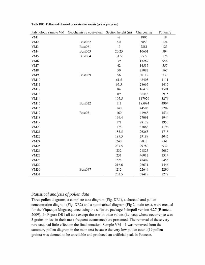
Table DR1. Pollen and charcoal concentration counts (grains per gram)

Palynology sample VM Geochemistry equivalent Section height (m) Charcoal /g Pollen /g

VM1 -2 1805 18VM2 Bdst062 6.8 5853 124 VM3 Bdst061 13 2881 123 VM4 Bdst063 20.25 10601 594 VM5 Bdst064 31.5 8577 125VM6 39 15289 956VM7 42 14537 557 VM8 50 25082 567 VM9 Bdst069 56 30119 737 VM10 61.5 48405 1111VM11 67.5 28665 1415VM12 84 16478 1591 VM13 89 36443 2915 VM14 107.5 117929 3276 VM15 Bdst022 111 185994 4904VM16 140 44503 2207VM17 Bdst031 160 41968 1534 VM18 166.4 27091 1944 VM19 171 28178 1953 VM20 178 87863 1196VM21 183.5 26263 1715 VM22 189.5 29189 2045 VM24 240 9818 661 VM25 237.5 29780 932VM26 232 21825 2087VM27 231 46012 2314 VM28 228 47407 2455 VM29 216.6 26631 1446 VM30 Bdst047 212 22649 2290VM31 203.5 58419 2272

Statistical analysis of pollen data Three pollen diagrams, a complete taxa diagram (Fig. DR1), a charcoal and pollen concentration diagram (Fig. DR2) and a summarised diagram (Fig 2, main text), were created for the Viqueque Megasequence using the software package Psimpoll version 4.27 (Bennett, 2009). In Figure DR1 all taxa except those with trace values (i.e. taxa whose occurrence was 3 grains or less in their most frequent occurrence) are presented. The removal of these very rare taxa had little effect on the final zonation. Sample VM – 1 was removed from the summary pollen diagram in the main text because the very low pollen count (19 pollen grains) was deemed to be unreliable and produced an artificial peak in Poaceae.

Acacia

Acera

ceae Aga

this

Alispo

rites Ant

hoce

ros

Arauc

ariac

eae

Areca

ceae Aste

race

ae Avicen

niaCala

mus Call

itris Cam

ptos

tem

non

Casua

rinac

eae

Ginkgo

acea

e

Cheno

podia

ceae

Cunon

iacea

e

Cyath

ea Cyper

acea

eDac

ryca

rpus

Dacry

dium

Drose

ra Elaeoc

arpa

ceae

Ericac

eae

Ficus Gleich

enia

Histiop

teris

Hymen

ophy

llace

ae

Hypole

pis a

mau

rora

chis

Jugla

ndac

eae

Liliac

eae

Lyco

podia

ceae

Lygo

dium M

alvac

eae

Mon

olete

fern

Mor

acea

e Myr

tace

ae Nypa

Ophiog

lossu

m

Panda

nace

ae

Passif

lorac

eae

Phyllo

cladu

s

Pinace

ae Planta

ginac

eae

Poace

ae

Podoc

arpa

ceae

Podoc

arpu

s

Polypo

diisp

orite

s

Polypo

dium

Prote

acea

e

Pterid

ium

Restio

nace

ae

Rhizop

hora

Sapind

acea

e

Sapot

acea

e

Selag

inella

Sphag

nace

ae

Spinele

ss A

stera

ceae

Thym

elaea

ceae

Trigl

ochin Tr

ilete

fern

Typh

a Uniden

tifiab

le

Zygop

hylla

ceae

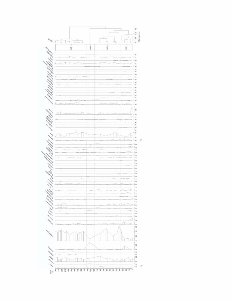
Fig. DR1: (previous page) A pollen diagram for the Viqueque Megasequence with including all taxa with at least a count of three grains on one level. Zonation is derived from CONISS within Psimpoll. Pollen types are in alphabetic order.

Zonation

Zonation based on cluster analysis was performed (Figs. DR1 and DR2). Subdivision of a pollen diagram into zones allows sections of similar fossil content to be grouped, and therefore, patterns of change through time to be identified. The pollen record was zoned using constrained cluster analysis by sum-of-squares (CONISS) as an option within Psimpoll (Bennett, 2009). CONISS clusters sample levels that are highly similar but is constrained to stratigraphically adjacent samples for division (Grimm, 1987).

Fig. DR2: Summarised pollen concentration and charcoal diagram.

Principal Component Analysis

Principal component analysis (PCA) is a multivariate analytical method that defines dimensionality in data sets (e.g. Abdi & Williams, 2010). The first principal component represents the strongest trend in the data, and axes thereafter are constrained to be orthogonal to the previous axis (Abdi & Williams, 2010). Three PCA analyses were performed using Canoco version 4.5 (ter-Braak & Smilauer, 2002) to visualize trends in the data.

PCA1:AlltaxaThe first PCA analysis included all taxa and had numerous rare taxa clustered at the centre of the chart (Fig. DR3). Araucariaceae (7) form the principal axis but the overall diagram is very noisy.

Fig. DR3: Principal Component Analysis for species of all taxa for VM pollen record. Species code 1 Acacia (Mimosaceae); 2 Aceraceae; 3 Agathis; 4 Alisporites (Gymnospermopsida); 5 Anthoceros (Anthocerotaceae); 6 Araucaria; 7 Araucariaceae; 8 Arecaceae; 9 Asteraceae; 10 Avicennia; 11 Calamus; 12 Callitris (Cupressaceae); 13 Camptostemon schultzii (Bombacaceae); 14 Casuarinaceae; 15 Ginkgoaceae; 16 Chenopodiaceae; 17 Cunoniaceae; 18 Cyathea; 19 Cyperaceae; 20 Dacrycarpus; 21 Dacrydium; 22 Drosera (Droseraceae); 23 Elaeocarpaceae; 24 Ericaceae; 25 Ficus (Moraceae); 26 Gleichenia (Gleicheniaceae); 27 Histiopteris (Dennstaedtiaceae); 28 Hymenophyllaceae; 29 Hypolepis amaurorachis (Dennstaedtiaceae); 30 Juglandaceae; 31 Liliaceae; 32 Lycopodiaceae; 33 Lygodium (Schizaeaceae); 34 Malvaceae; 35 Monolete fern; 36 Moraceae; 37 Myrtaceae; 38 Nypa fruticans (Arecaceae); 39 Ophioglossum (Ophioglossaceae); 40 Pandanaceae; 41 Passifloraceae; 42 Phyllocladus; 43 Pinaceae; 44 Plantaginaceae; 45 Poaceae; 46 Podocarpaceae; 47 Podocarpus; 48 Polypodiisporites (Polypodiaceae); 49 Polypodium (Polypodiaceae); 50 Proteaceae; 51 Pteridium (Dennstaedtiaceae); 52 Restionaceae; 53 Rhizophora; 54 Sapindaceae; 55 Sapotaceae; 56 Selaginella (Sellaginaceae); 57 Sphagnaceae; 58 Spineless asteraceae; 59 Thymelaeaceae; 60 Triglochin (Juncaginaceae); 61 Trilete fern; 62 Typha (Typhaceae); 63 Unidentifiable; 64 Zygophyllaceae.

PCA2:SummarisedTaxa,ExcludingSampleVM‐1The second PCA analysis excluded rare species and combined pteridophytes such as Lycopodiaceae and Cyatheaceae into a single category of ‘Ferns’ [sic] to reduce noise. Sample VM – 1 was also removed from the second PCA analysis due to low pollen counts which produced a bias toward Poaceae based on the very low count in this sample. This PCA analysis again highlighted Araucariaceae on the first principal component but the rest of the

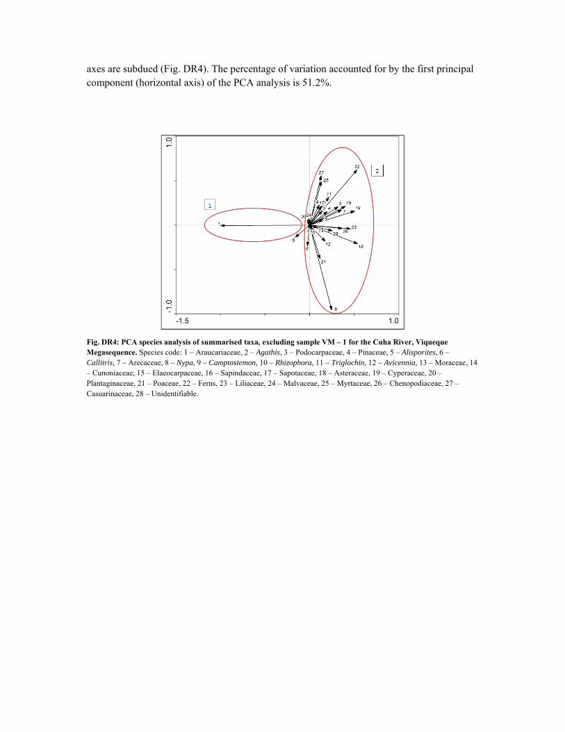
axes are subdued (Fig. DR4). The percentage of variation accounted for by the first principal component (horizontal axis) of the PCA analysis is 51.2%.

Fig. DR4: PCA species analysis of summarised taxa, excluding sample VM – 1 for the Cuha River, Viqueque Megasequence. Species code: 1 – Araucariaceae, 2 – Agathis, 3 – Podocarpaceae, 4 – Pinaceae, 5 – Alisporites, 6 – Callitris, 7 – Arecaceae, 8 – Nypa, 9 – Camptostemon, 10 – Rhizophora, 11 – Triglochin, 12 – Avicennia, 13 – Moraceae, 14 – Cunoniaceae, 15 – Elaeocarpaceae, 16 – Sapindaceae, 17 – Sapotaceae, 18 – Asteraceae, 19 – Cyperaceae, 20 – Plantaginaceae, 21 – Poaceae, 22 – Ferns, 23 – Liliaceae, 24 – Malvaceae, 25 – Myrtaceae, 26 – Chenopodiaceae, 27 – Casuarinaceae, 28 – Unidentifiable.

PCA3:SummarisedTaxa,ExcludingVM–1andAraucariaceaeA third PCA analysis was performed on the summarised taxa, excluding sample VM- 1 and Araucariaceae counts (apart from Agathis pollen grains). This was undertaken to explore trends that were hidden from the previous analysis by the dominance of the Araucariaceace. The first and second principal components of species (Fig. DR5) of the third PCA are equivalent to the second and third principal component of the second PCA. This analysis allows swamp-mangrove (box 1), lowland forest (box 2), sclerophyll forest (box 3) and less convincingly, lowland rainforest (box 4) to be distinguished.

Fig. DR5: PCA species analysis for summarised taxa, excluding VM – 1 and the taxa Araucariaceae for the Cuha River, Viqueque Megasequence. Boxes 1-4 represent mangrove, lowland forest, sclerophyll forest and lowland rainforest respectively. Species code: 2 – Agathis, 3 – Podocarpaceae, 4 – Pinaceae, 5 – Alisporites, 6 – Callitris, 7 – Arecaceae, 8 – Nypa, 9 - Camptostemon, 10 – Rhizophora, 11 – Triglochin, 12 – Avicennia, 13 – Moraceae, 14 – Cunoniaceae, 15 – Elaeocarpaceae, 16 – Sapindaceae, 17 – Sapotaceae, 18 – Asteraceae, 19 – Cyperaceae, 20 – Plantaginaceae, 21 – Poaceae, 22 – Ferns, 23 – Liliaceae, 24 – Malvaceae, 25 – Myrtaceae, 26 – Chenopodiaceae, 27 – Casuarinaceae.

Geochemistrymethodsanddata

Samples from the type section were analysed to determine weight loss on ignition, major and trace element geochemistry and XRD mineralogy. Loss on ignition (LOI) refers to the weight loss of a sample following combustion in a furnace and is dependent on temperature and duration of combustion. Different temperatures of combustion affect different changes in the composition of the sediment. Loss on ignition at 550°C (LOI550) is generally considered to be proportional to the total organic carbon content of the sediment (Dean, 1974) but may also be contributed to by the loss of structural water in clay, which may account for <20% weight loss in clay rich samples (Mook and Hoskin, 1982; Santisteban et al., 2004). Although total organic carbon generally has a mixed marine/continental signature (e.g. McKirdy and Cook, 1980, DSDP 262), the LOI550 stratigraphy in a section is sensitive to changes in depositional setting, particularly as part of an integrated study that incorporates mudstone geochemistry. The dominant factor that causes weight loss in carbonates between 550-1,000°C (reported as LOI1000) is the loss of carbonate CO2, such that carbonate content can be estimated from LOI1000. When this relationship is used, carbonate estimation error is proportional to clay content and inversely proportional to carbonate content (Santisteban et al., 2004). Wt % carbonate calculated from LOI for clay rich rocks should therefore be viewed with caution.

Loss on ignition Samples of 12-15 g were air dried and ground to powder in a Rocklabs tungsten carbide ring mill. The samples were oven dried for a minimum of 24 hours at 105°C to remove water and achieve a stable dry weight. The dried powder was decanted into pre-weighed porcelain crucibles. The filled crucibles were reweighed to determine dry weight (DW105) then burnt for exactly two hours at 550°C in a thermostat-controlled Barnstead Thermolyne 1400 muffle furnace. The weight percentage organic carbon was estimated as the weight loss on ignition at 550°C (LOI550 ), which was calculated following Heiri et al. (2001) as:

whereDW105andDW550arethesampleweightsbeforeandafterburningat550°Crespectively.

X-ray fluorescence spectrometry The ashed LOI samples were used to produce XRF samples, which were analyzed at the University of Canterbury Geological Sciences Department using a Phillips PW2400 Sequential Wavelength Dispersive X-ray Fluorescence Spectrometer. The spectrometer is calibrated using sets of international standards which have been certified.

Rock majors including SiO2, TiO2, Al2O3, Fe2O3T, MnO, MgO, CaO, Na2O, K2O, and P2O5 were analysed by fused disc. Glass fusion beads were prepared by fusing together approximately 1.3g of rock powder with 6.98g of flux (Li2B4O7 and Li2O mixture) and a few grains of oxidant (NH4NO3) at 1130 ˚C for at least 15 minutes in Pt/Au crucibles. Loss on ignition was calculated after fusion. Glass beads were formed by pouring the molten material into Pt/Au moulds which are cooled rapidly (for rock majors analysis).

LOI550

Trace elements were analysed by pressed powder pellet. The 32mm diameter pressed powder pellets were prepared using approximately 8g of rock powder and polyvinyl alcohol solution as a binder. The pellets are pressed in a hardened steel die at 3000 psi for 10 seconds.

XRD analysis Duplicate samples were ground in an agate mortar and pestle with the addition of ethanol to form a slurry. The slurry was transferred to half a microscope slide as a thin layer (orientated mount) using a disposable pipette and allowed to dry at room temperature. The mineralogy of crystalline components of the samples was determined using a Philips PW1729 X-ray generator (50kV/40mA), equipped with a PW2273/20 long fine focus 2.2kW Cu anode x-ray tube, a PW 1820 goniometer, a PW1752 monochromator, a PW1711 sealed gas (Xe) filled proportional detector and a PW1710 diffractormeter control connected to a PC. The PC was loaded with Visual XRD controller software and Traces (V4) search-match software using the Hanawalt search-match algorithm. Peak areas of each identified phase were measured to estimate relative amounts. The samples were scanned from 3° to 70° 2θ with a step size of 0.02° 2θ and scan speed of 0.02° 2θ per second. For determination of swelling/expanding clay mineral content, the air dried slides were placed into a desiccator with ethylene glycol solution overnight in an oven at 60˚C. Once the slides had cooled to room temperature they were scanned from 3° to 30° 2θ. For clay minerals affected by heat the glycolated slides were placed into a muffle furnace for one hour at 550˚C. Once the slides had cooled to room temperature they were scanned from 3 to 30 ° 2θ.

Collated geochemistry data is presented in Table DR2.

Table DR2. Geochemistry results

Sample No: TS060 TS062 TS061 TS063 TS064 TS069 TS011 TS018 TS022 TS027 TS031 TS035 TS042 TS047

Pollen sample:

vm2 vm3 vm4 vm5 vm9 vm12 vm15 vm17

vm30

Section height 0.1 7 13 20.5 31.5 56 71.5 89 111 139 160 176 197 212.5

Major elements wt%

SiO2 5.57 18.97 26.35 33.14 28.71 47.18 50.6 43.59 42.26 42.09 43.94 49.69 48.27 55.14

TiO2 0.06 0.26 0.34 0.4 0.39 0.72 0.77 0.66 0.61 0.65 0.68 0.76 0.73 0.87

Al2O3 1.39 5.61 7.09 8.51 7.69 13.51 12.03 12.95 12.4 11.39 11.85 15.3 13.51 15.28

Fe2O3 0.6 2.32 3 3.63 3.61 6.53 5.66 6.75 7.44 6.25 4.94 7.68 8.5 6.44

MnO 0.07 0.11 0.07 0.09 0.1 0.17 0.13 0.82 0.83 0.28 0.15 0.24 0.51 0.16

MgO 0.46 1.51 2.26 1.93 3.95 3.32 2.74 3.13 3 2.75 2.47 3.13 3.24 3.38

CaO 50.81 38.56 32.13 28.11 27.4 13.14 13.48 15.11 15.88 18.01 17.84 10.25 11.36 7.64

Na2O 0.16 0.29 0.35 0.75 0.37 1.06 1.21 0.6 0.56 1.03 1.05 1.02 0.95 1.28

K2O 0.22 0.89 1.16 1.32 1.35 2.3 1.82 2.28 2.27 1.85 1.89 2.46 2.23 2.43

P2O5 0.03 0.13 0.13 0.13 0.13 0.15 0.14 0.15 0.17 0.17 0.16 0.16 0.18 0.13

LOI550 1.24 3.31 5.21 6.63 4.54 6.18 4.58 6.48 6.86 4.85 4.47 6.08 7.22 6.14

LOI1000 40.23 30.56 25.8 20.49 25.2 10.89 11.14 13.43 14.02 14.66 14.48 8.89 10.07 6.93

Roser and Korch (1988) discriminant function values

R&K F1 -1.06 -1.94 -1.49 -2.08 -0.15 -2.04 -2.08 -2.79 -3.60 -2.91 -1.61 -3.16 -4.17 -1.66

R&K F2 5.21 4.02 5.61 2.37 11.42 2.92 2.78 2.49 1.62 2.14 2.55 1.20 1.18 2.89

XRD mineralogy

Quartz TR 5 10 10 20 50 50 45 35 45 35 55 60

Albite 10 10 tr 5 5 5 10 10

Calcite 100 95 90 90 80 40 40 55 60 50 60 30 25

Kaolinite TR TR TR TR TR TR 5 5

Trace elements (ppm)

V 24 67 84 81 79 144 122 134 119 123 126 152 151 157

Cr 14 76 65 52 84 124 108 138 115 115 120 154 121 132

Ni 9 35 39 44 34 62 50 66 53 41 63 51 42 57

Zn 18 59 74 81 71 107 92 100 89 94 102 103 97 110

Zr 28 64 80 91 88 143 158 128 122 125 133 145 139 168

Nb 3 6 7 7 8 15 15 12 12 13 14 16 14 16

Ba 543 293 232 366 458 373 373 544 355 367 359 425 457 418

La 2.5 20 21 22 18 32 27 24 24 23 19 30 26 29

Ce 14 31 29 32 27 52 46 48 47 39 55 50 53 59

Nd 13 19 43 5 23 31 5 30 10 27 49 34 32 48

Ga 3 7 10 10 11 17 15 17 16 15 15 20 17 19

Pb 2 5 4 6 3 15 13 7 12 10 12 17 13 18

Rb 6 38 50 53 63 108 86 105 104 86 89 121 104 116

Sr 920 1143 1217 1176 1121 681 562 709 693 704 709 444 526 358

Th 0.5 4 2 5 3 10 8 10 11 7 9 13 10 13

Y 7 16 19 21 17 28 27 25 23 24 25 30 28 29

DerivationofSectionagemodel

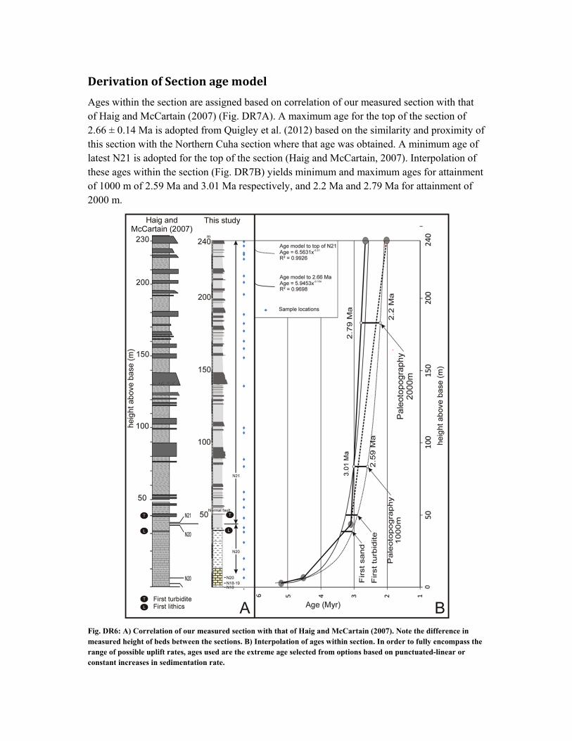
Ages within the section are assigned based on correlation of our measured section with that of Haig and McCartain (2007) (Fig. DR7A). A maximum age for the top of the section of 2.66 ± 0.14 Ma is adopted from Quigley et al. (2012) based on the similarity and proximity of this section with the Northern Cuha section where that age was obtained. A minimum age of latest N21 is adopted for the top of the section (Haig and McCartain, 2007). Interpolation of these ages within the section (Fig. DR7B) yields minimum and maximum ages for attainment of 1000 m of 2.59 Ma and 3.01 Ma respectively, and 2.2 Ma and 2.79 Ma for attainment of 2000 m.

Fig. DR6: A) Correlation of our measured section with that of Haig and McCartain (2007). Note the difference in measured height of beds between the sections. B) Interpolation of ages within section. In order to fully encompass the range of possible uplift rates, ages used are the extreme age selected from options based on punctuated-linear or constant increases in sedimentation rate.

SUPPLEMENTARY REFERENCES

Abdi, H., and Williams, L.J., 2010, Principal Component Analysis, Wiley Interdisciplinary Reviews: Computational Statistics, v. 2, p. 433-459.

APSA Members, 2007, The Australasian Pollen and Spore Atlas, Canberra, Australia, Australian National University.

Bennett, K. D., 2009, Documentation for psimpoll 4.27 and pscomb 1.03. C programs for plotting and analyzing pollen data: The 14Chrono Centre, Archaeology and Palaeoecology.

Dean, W. E., 1974, Determination of carbonate and organic matter in calcareous sediments and sedimentary rocks by loss on ignition: Comparison with other methods: Journal of Sedimentary Petrology, v. 44, p. 242-248.

Fægri, K., and Iversen, J., 1989, Textbook of Pollen Analysis, New York, John Wiley and Sons. Inc, 328 p.:

Grimm, E.C., 1987, CONISS: A FORTRAN 77 program for stratigraphically constrained cluster analysis by the method of incremental sum of squares, Computers & Geoscience, v. 13, p. 13-35.

Haig, D. W., and McCartain, E., 2007, Carbonate pelagites in the post-Gondwana succession (Cretaceous - Neogene) of East Timor: Australian Journal of Earth Sciences, v. 54, no. 6, p. 875-897.

Heiri, O., Lotter, A. F., and Lemcke, G., 2001, Loss on ignition as a method for estimating organic and carbonate content in sediments: reproducibility and comparability of results: Journal of Paleolimnology, v. 25, no. 1, p. 101-110.

Hopf, F., Shimeld, P., and Pearson, S., 2005, The Newcastle Pollen Collection, School of Environmental and Life Sciences at the University of Newcastle, Australia (http://www.aqua.org.au/AQUA/Pollen/).

Jarzen, D. M., and Nichols, D. J., 1996, Pollen, in Jansonius, J., and McGregor, D. C., eds., Palynology: Principles and Applications, Volume 1, American Association of Stratigraphic Palynologists Foundation, p. 261-291.

Kneller, M., 2009, Pollen Analysis, in Gornitz, V., ed., Encyclopedia of Paleoclimatology and Ancient Environments: Netherlands, Springer, p. 815-823.

McKirdy, D. M., and Cook, P. J., 1980, Organic Geochemistry of Pliocene-Pleistocene Calcareous Sediments, DSDP Site 262, Timor Trough: American Association of Petroleum Geologists Bulletin, v. 64, p. 2118-2138.

Mook, D. H., and Hoskin, C. M., 1982, Organic determinations by ignition: Caution advised: Estuarine, Coastal and Shelf Science, v. 15, no. 6, p. 697-699.

Quigley, M.C., Duffy, B., Woodhead, J., Hellstrom, J., Moody, L., Horton, T., Suares, J., and Fernandes, L., 2012, U/Pb dating of a terminal Pliocene coral from the Indonesian Seaway: Marine Geology, v. 311-314, p. 57-62.

Raine, J. I., Mildenhall, D. C., and Kennedy, E. M., 2008, New Zealand Fossil Spores and Pollen: An Illustrated Catalogue, GNS Science (http://www.gns.cri.nz/what/earthhist/fossils/spore_pollen/catalog/index.htm).

Santisteban, J. I., Mediavilla, R., Lopez-Pamo, E., Dabrio, C. J., Blanca Ruiz Zapata, M., Jose Gil Garcıa, M., Castano, S., and Martınez-Alfaro, P. E., 2004, Loss on ignition: a qualitative or quantitative method for organic matter and carbonate mineral content in sediments?: Journal of Paleolimnology, v. 32, p. 287-299.

ter-Braak, C.J.F., and Šmilauer, P 2002, CANOCO Reference manual and CanoDraw for Windows User's guide: Software for Canonical Community Ordination (version 4.5), Microcomputer Power, New York, United States of America.

van der Kaars, W. A., 1991, Palynology of eastern Indonesian marine piston-cores: a Late Quaternary vegetational and climatic record for Australasia: Palaeogeography, Palaeoclimatology, Palaeoecology, v. 85, no. 3-4, p. 239-302.

Wang, X., van der Kaars, S., Kershaw, A.P., Bird, M. and Jansen, F. 1999. A record of fire, vegetation and climate through the last three glacial cycles from Lombok Ridge core G6-4, eastern Indian Ocean, Indonesia. Palaeogeography, Palaeoclimatology, Palaeoecology. v. 147, p. 241-256.