paddy rice experiment in the sanjiang plain (presp)

Paddy Rice Experiment in the

Sanjiang Plain (PRESP 2012)

Field Measurement Report

Version 1.0

Hongliang Fang, Wenjuan Li, Shanshan Wei, Tao Sun, Chongya Jiang

State Key Laboratory of Resources and Environmental Information System,

Institute of Geographic Sciences and Natural Resources Research,

Chinese Academy of Sciences

January 2014

Paddy Rice Experiment in the Sanjiang Plain Field Measurement Report

Version: 1.0 Date: January 2014 Page 1 of 32

Participants

Prof. Hongliang Fang

Principle Investigator

LREIS, Institute of Geographic Sciences and Natural Resources Research


Beijing 100101, China

Email: [email protected]

Wenjuan Li, Shanshan Wei, Tao Sun, Chongya Jiang

PhD. students



Beijing 100101, China

Acknowledgments

The field campaign was supported by the National Natural Science Foundation of

China (41171333) and the Hundred Talent Program of the Chinese Academy of

Sciences. We would like to thank the interns who attended the field work at various

stages, and the farmers for allowing us to make use of their fields for in situ

measurements.



Revision History

Revision Date Changes Major contributor

2014-1-20 Initial draft Wenjuan Li



Table of Contents

1. Overview .............................................................................................................. 7

2. Site description and ground sampling .............................................................. 8

2.1 Site description ............................................................................................ 8

2.2 Sampling strategy ........................................................................................ 8

3. Field measurements methods .......................................................................... 12

3.1 LAI-2200 ................................................................................................... 12

3.2 DHP ........................................................................................................... 14

3.3 AccuPAR ................................................................................................... 17

3.4 Destructive method ................................................................................... 18

4. Results ................................................................................................................ 21

4.1 Destructive PAI ......................................................................................... 21

4.2 Gap fraction............................................................................................... 22

4.3 Clumping index ......................................................................................... 22

4.4 ALA and fCover ........................................................................................ 23

5. Quality assurance ............................................................................................. 25

6. Data access and citation ................................................................................... 30

6.1 Data access ................................................................................................ 30

6.2 Citation ...................................................................................................... 30

References ................................................................................................................. 30



List of Figures

Fig. 1 Location of site and sampling strategy for a plot and within an ESU.

Fig. 2 Sample photos for the main growing stages.

Fig. 3 Radiation, PAR, temperature and relative humidity for the site in

2012.

Fig. 4 LAI-2200 with single sensor.

Fig. 5 Sampling strategy for LAI-2200 over paddy rice field.

Fig. 6 LAI-2200 field measurement method.

Fig. 7 Nikon D5100 equipped with Sigma F2.8 EX DC circular fisheye. An

ultraviolet cap was used to prevent dust or rain from the lens.

Fig. 8 (a) Downward-looking photos for low rice canopy (< 0.7 m, before

Jul 7). When rice grows higher (> 0.7 m, enter flowering stage), both

downward photos (b) and upward photos (c) are taken.

Fig. 9 An example of photo classification in CAN_EYE software. Green

indicates the rice and soil is the background. The operators have been

masked.

Fig. 10 AccuPAR model LP-80 PAR/LAI ceptometer.

Fig. 11 Below canopy PAR measurements in four directions with AccuPAR.

Fig. 12 Cut rice above the water (left) and preserve them in a cooler box

(right).

Fig. 13 Scan leaves and young stems by LI-3100C.

Fig. 14 Scanned stems in a scanner (left) and binaries them to collect pixels

area (right).

Fig. 15 Seasonal variation of LAI and PAI values calculated as the developed

surface area. The average data for five plots are presented in (f).

Fig. 16 Seasonal variation of the average gap fraction at different view zenith

angles from LAI-2200 and downward and upward DHPs. For DHPs,

the modeled effective gap fractions from CAN_EYE V6.1 are shown.

Fig. 17 Seasonal variation of the average clumping indices from, (a) the

downward DHP, (b) the upward DHP and (c) LAI-2200. Panel (d)

shows the angular average of CI values.

Fig. 18 Seasonal variation of ALA calculated from LAI-2200, downward

DHP and upward DHP. Solid and dashes lines represent true and

effective ALAs retrieved from DHPs, respectively.

Fig. 19 Seasonal variation of fCover calculated from LAI-2200, downward

DHP and upward DHP.



List of Tables

Table 1 Structural variables derived from field measurement methods.

Table 2 Information for the five plots in the study area.

Table 3 The weighting factors of each ring for LAI-2200 and LAI-2000.

Table 4 Major morphological changes, rice height, water depth and

instruments conditions during the measurement.



List of Acronyms and Abbreviations

ACFs Apparent clumping factors

ALA Average leaf angle

CI Clumping index

DHP Digital hemispheric photography

DOY Day of year

ESU Elementary sampling unit

fCover Fraction of vegetation cover

LAI Leaf area index

LAD Leaf angle distribution

LAI-2200 4R LAI-2200 with the inner four rings

LAI-2200 5R LAI-2200 with all five rings

LUT Look up table

PAI Plant area index

PAIeff Effective plant area index

PAR Photosynthetically active radiation

SAI Stem and seeds area index

SZA Solar zenith angle

VALERI Validation of Land European Remote Sensing Instruments

VZA View zenith angle

YAI Yellow area index



1. Overview

The Paddy Rice Experiment in the Sanjiang Plain (PRESP) was conducted at the

paddy rice fields in Honghe Farm, NE China (47°39.11′ N，133°31.31′ E), from

mid-June to mid-September 2012. The objective of the field campaign is to collect

consistent ground LAI data for paddy rice in order to support the validation of LAI

products obtained by remotely sensed data. The site is about 3 km × 3 km with five

plots scattered in four corners and the center. Several optical instruments, including

LAI-2200, Digital Hemispheric Photography (DHP), and AccuPAR and the

destructive methods were used to obtain LAI and other structural parameters (Table

1).

Table 1. Structural variables derived from field measurement methods.

LAI-2200 DHPs AccuPAR Destructive

PAI √ √

PAIeff √ √ √

LAI √

YAI √

SAI √

Angular Gap fraction √ √

Integrated gap fraction

or transmittance √ √ √

CI √ √

ACF √

ALA √ √

fCover √ √



2. Site description and ground sampling

2.1 Site description

The study area is located at the Honghe Farm in the Heilongjiang Province, NE China

(Fig. 1). The site experiences a typical humid continental monsoon climate, with long

cold winter and warm and humid summer. The mean annual temperature is 2.52°,

with monthly mean temperature ranging from -20° in January to about 22° in July.

The average annual precipitation is approximately 558 mm, with substantial

interannual and seasonal variation (Song et al., 2009). The mean altitude of this site is

approximately 56 m. The main soil types are the albic bleached meadow soils

(Albaqualfs) (Yang et al., 2013). The water and soil in these marshes are completely

frozen from late October to April and begin to thaw in late April.

This site was originally a wetland and has been converted to plant paddy rice since

1997. The paddy rice fields are flat with more than 5 km homogeneity and large

rectangular fields approximately 30 m 100 m in size. A single rice variety

(Japonica) is grown in this region. The rice-cropping practices are uniform, growing

once a year during the summer season (May to September), with a maturation stage

for about 120-150 days. The dates for the panicle formation stage, heading stage, and

maturity stage are mid-June, mid-July, and early August, respectively. Paddy fields

are irrigated with ground water throughout the season. The soil surface is under

flooded conditions during most of the growing periods.

2.2 Sampling strategy

Five plots (A, B, C, D, and E), four at the four corners and one at the center, were

chosen for intensive ground based measurements (Fig. 1). Each plot was planted with

a cultivar type and managed individually. Small differences exist among the plots in

terms of the plant density and plantation methods (Table 2). Within each plot, 50 ~ 60

Elementary Sampling Units (ESUs), in the size of 1515 m2 or 20 20 m2 were

selected. ESUs were located at least 1.5 m away from the field borders. The main

information of five plots is showed in Table 2.

In order to reduce the impact of destructive sampling and measurement disturbance, a

moving sampling strategy was adopted. Four ESUs within a plot were selected in the

first week and LAI measurements were taken for each ESU using one method. Used

ESUs will be discarded and another four parallel ESUs will be selected for the next

week. ESU-level sampling was performed along a diamond box with two 15-meter

diagonals as recommended by the VALERI network (Validation of Land European

Remote Sensing Instruments,

http://w3.avignon.inra.fr/valeri/).

http://w3.avignon.inra.fr/valeri/



Fig. 1 The upper panel shows the location of the site on BingTM images, a photo

taken in a paddy rice field and the distribution of five plots on a Landsat-7 ETM+

image (June 3, 2012). The middle panel shows the seasonal sampling strategy for a

plot and within an ESU for LAI-2200, AccuPAR and DHP (‘W’ represents week).

The bottom panel shows the downward DHP images obtained during different stages

of leaf development.



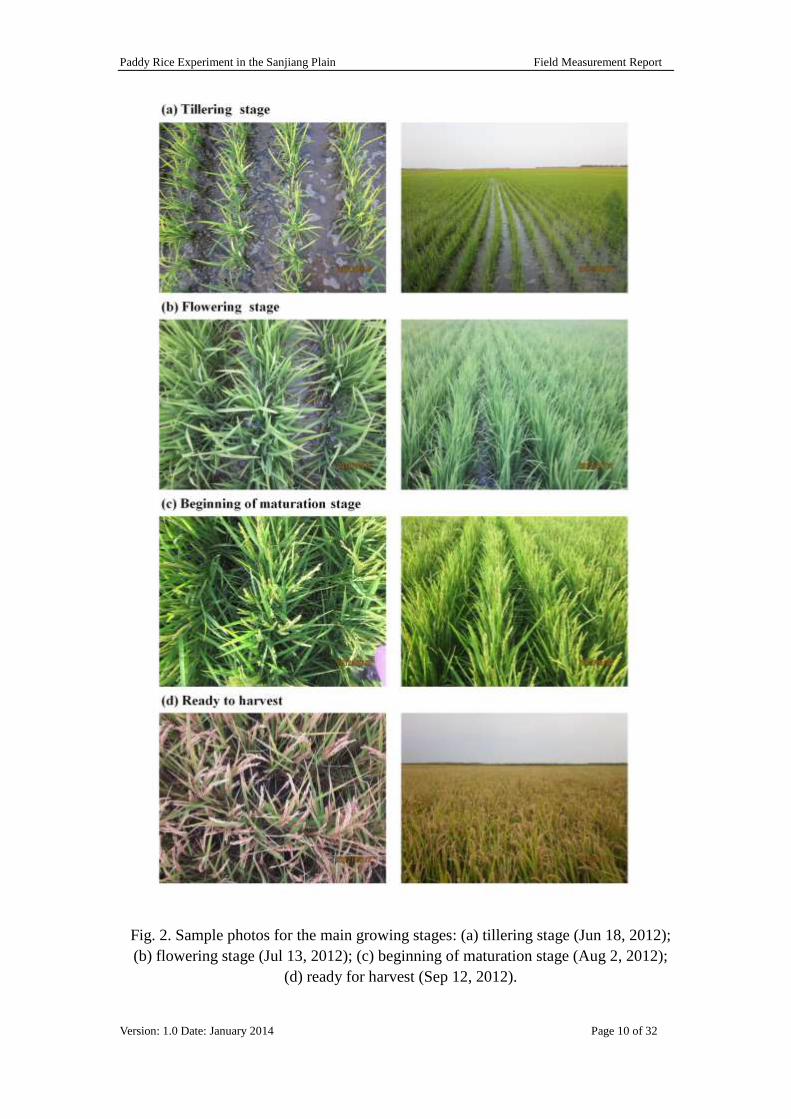
Fig. 2. Sample photos for the main growing stages: (a) tillering stage (Jun 18, 2012);

(b) flowering stage (Jul 13, 2012); (c) beginning of maturation stage (Aug 2, 2012);

(d) ready for harvest (Sep 12, 2012).



Table 2. Information for the five plots in the study area.

Ground LAI measurement was conducted from June 11, shortly after the rice

transplantation, to September 17 when the rice was ready for harvest. Fig. 2 shows

some photos taken at the main growing stages in the study area. Field measurements

were performed sequentially for the five plots every week, in order to capture the

canopy structural dynamics. All optical measurements were conducted near sunset or

under overcast conditions as the sensitivity of the parameters and the retrieval errors

increase under direct illuminations (Garrigues et al., 2008). Major morphological

changes, rice height, water depth and field conditions during this period were also

observed and recorded (Table 4). The radiation, PAR, temperature, and relative

humidity were obtained at a nearby weather station managed by the Sanjiang Marsh

and Wetland Ecological Experiment Station, Chinese Academy of Sciences (Fig. 3).

Fig. 3. Radiation, PAR, temperature, and relative humidity for the site in 2012.

Plot ID Center location Density

(plants/m2)

Inter-row

distance (m)

ESU size

(m)

A 133.515°E, 47.667°N 25 0.288 10×10

B 133.532°E, 47.663°N 26 0.286 10×10

C 133.523°E, 47.653°N 24 0.299 15×15

D 133.515°E, 47.637°N 28 0.283 15×15

E 133.534°E, 47.637°N 28 0.274 15×15



3. Field measurement methods

3.1 LAI-2200

A LAI-2200 Plant Canopy Analyzer (PCA) (LI-COR Inc., Lincoln, Nebraska) was

used to estimate the rice PAI as all parts of the plants, including green leaves, yellow

leaves, stems, and seeds contribute to the canopy transmittance process (Fig. 4). All

measurements were conducted under diffuse conditions. Following the instruction

manual for row crops, ground measurements were made along diagonal transects

between the rows (Fig. 5). Two repeats were made for each measurement with one

above and four below canopy readings (Fig. 6). For below canopy measurements, the

instrument was held about 5 cm above the background soil or shallow water.

Throughout the season, a 270° view cap was used to shield the sensor from the

operator. All values from four measurements were averaged to obtain the values at the

ESU level.

Fig. 4. LAI-2200 with a single sensor Fig. 5. Sampling strategy for LAI-2200

over paddy rice field

Fig. 6. LAI-2200 field measurement method (left: above the canopy;

right: below the canopy)



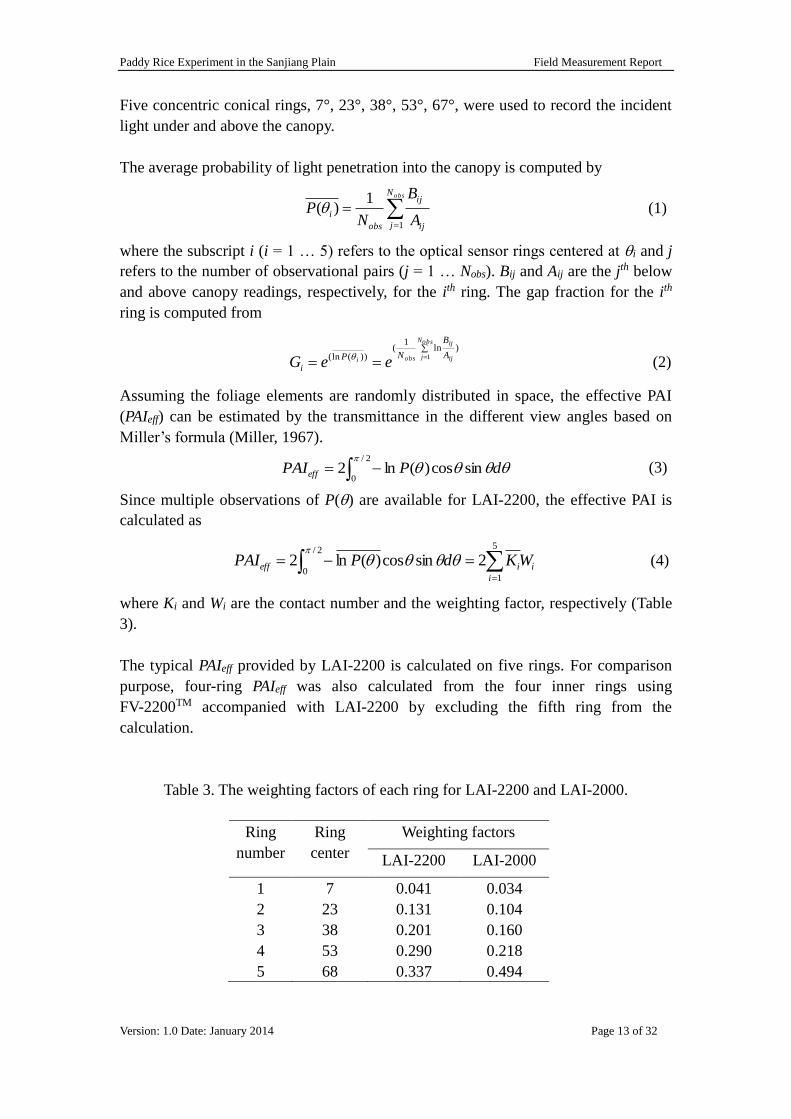
Five concentric conical rings, 7°, 23°, 38°, 53°, 67°, were used to record the incident

light under and above the canopy.

The average probability of light penetration into the canopy is computed by

obsN

j ij

ij

obs

iA

B

NP

1

1)( (1)

where the subscript i (i = 1 … 5) refers to the optical sensor rings centered at i and j

refers to the number of observational pairs (j = 1 … Nobs). Bij and Aij are the jth below

and above canopy readings, respectively, for the ith ring. The gap fraction for the ith

ring is computed from

)ln1

())(ln( 1

obsN

j ij

ij

obsiA

B

NP

i eeG

(2)

Assuming the foliage elements are randomly distributed in space, the effective PAI

(PAIeff) can be estimated by the transmittance in the different view angles based on

Miller’s formula (Miller, 1967).

2/

0sincos)(ln2

dPPAIeff (3)

Since multiple observations of P() are available for LAI-2200, the effective PAI is

calculated as

5

1

2/

02sincos)(ln2

i

iieff WKdPPAI

(4)

where Ki and Wi are the contact number and the weighting factor, respectively (Table

3).

The typical PAIeff provided by LAI-2200 is calculated on five rings. For comparison

purpose, four-ring PAIeff was also calculated from the four inner rings using

FV-2200TM accompanied with LAI-2200 by excluding the fifth ring from the

calculation.

Table 3. The weighting factors of each ring for LAI-2200 and LAI-2000.

Ring

number

Ring

center

Weighting factors

LAI-2200 LAI-2000

1 7 0.041 0.034

2 23 0.131 0.104

3 38 0.201 0.160

4 53 0.290 0.218

5 68 0.337 0.494



Compared to the LAI-2000, LAI-2200 has changed the weighting factors for the five

rings (Table 3). Moreover, LAI-2200 provides the Apparent Clumping Factor (ACFs)

using the gap fraction measured by five rings (Ryu et al., 2010). ACFs has been

considered representing the maximum clumping index for canopy.

5

1

5

1

2/

0

2/

0

2

)(ln2

sin)(

)(ln2

sin)(

)(ln2

i

ii

i

i

i

i

s

WK

WS

P

dS

P

dS

P

ACF

(5)

LAI-2200 calculates the foliage mean tilt angle based on Lang (1986), using an

empirical polynomial relating inclination angle to the slopes of the idealized curves

between 25° and 65°.

The fractional vegetation cover (fCover) is calculated by:

)7(1 PfCover (6)

where )7( P is the gap fraction measured on the first ring center at 7°.

3.2 DHP

The DHP images were taken using a Nikon D5100 camera and a 4.5 mm F2.8 EX DC

circular fisheye convertor (Fig. 7). An ultraviolet cap was used to prevent dust or rain

from the lens. The total height of camera and the lens was about 16.5 cm. Two bubble

levels were attached to the camera to keep it horizontal for both downward and

upward viewing directions. System calibration for DHP camera was performed before

measurement according to the CAN_EYE manual (version 6.3.3), in order to get the

optical center and projection function of the lens (Weiss and Baret, 2010).

Fig. 7. Nikon D5100 equipped with Sigma F2.8 EX DC circular fisheye. An

ultraviolet cap was used to prevent dust or rain from the lens.



Downward-looking photos were taken before July 10 (DOY 192) when the rice began

to enter the flowering stage (Fig. 8a). The distance between the camera and the top

canopy was set to about 0.8-1.5 m to avoid individual leaves too close to the camera.

When the rice grew higher than 70 cm (after July 10), upward-looking photos were

also taken at the same location of the downward measurements (Fig. 8b and 8c). For

the upward measurements, the camera was placed right above the ground soil or water.

Before July 26 (DOY 208), the camera was set to automatic exposure to prevent the

saturation issues during the downward measurement (Demarez et al., 2008). After that,

the aperture and shutter speed of the camera were manually adjusted to avoid

over-exposure because the sunlight intensity may change greatly during the

measurement direction shifts. To properly sample the spatial variability of the ESU, at

least 20 hemispherical photos with single direction were taken along the diamond

strategy (Fig. 1). Nearly all photos were taken under overcast illumination to

minimize the shadow effect. All images within an ESU were considered to be under

similar illumination conditions. These photos were stored in high-quality JPEG

format at a resolution of 32644928.

Fig. 8. (a) Downward-looking photos for low rice canopy (< 0.7 m, before Jul 7).

When rice grew higher (> 0.7 m, enter flowering stage), both downward photos (b)

and upward photos (c) were taken.



All valid photos (8~20) over one ESU were processed simultaneously by the

CAN_EYE software (version 6.3.3) to extract the structural variables (Weiss et al.,

2004). The limit of image in viewing degrees used in this research (COI) was set to

60° by default. To get a balance between the computation time and images amount,

angular resolution for zenith and azimuth directions were set to 10° and the solid

angle used in computing the cover fraction was also set to 10°. A threshold process is

necessary to separate the foliage from the soil background (downward view) or the

sky (upward view). To minimize subjective errors, one operator performed all

thresholding and classification processes. Fig. 9 presents an example for the

downward DHPs classification results in CAN_EYE. More detailed processing

procedures can be found in the CAN_EYE manual (version 6.3.3).

Fig. 9. An example of photo classification in the CAN_EYE software. Green indicates

the rice and soil is the background. The operators have been masked.

Assuming an ellipsoidal distribution of the leaf inclination, PAIeff is retrieved using

look-up-table techniques with CAN_EYE (Weiss and Baret, 2010). A large range of

random combinations of LAI (0 ~ 10) and ALA (10° ~ 80°) values are used to build a

database following the Beer-Lambert’s law (Nilson, 1971):

)cos(/)(

)(

effPAIGeP

(7)

where P() is the canopy gap fraction at direction and G() is the projection

function. By comparing the measured gap fraction and those stored in look-up-table,

effective PAI and ALA can be retrieved from Eq. (7) by setting a cost function.



The regularization cost functions used in CAN-EYE V5.1 (Eq. 7 in Weiss 2010) and

V6.1 (Eq. 8 in Weiss 2010) are different. V5.1 tries to constrain the retrieved ALA to

be within 60° 30°, whereas V 6.1 tries to minimize the difference between the

retrieved PAI and that estimated from the 57° observations. The constraints on V6.1

are efficient without any assumption on ALA; therefore, the V6.1 results are mainly

considered for further analysis in this report.

The clumping index (CI) at direction is computed using the logarithm gap fraction

averaging method (Lang and Xiang, 1986):

)(ln

)(ln)(

P

PCI (8)

The fraction of vegetation cover (fCover) is calculated as the fraction of the soil

covered by the vegetation viewed in the nadir direction.

)(1 minPfCover (9)

where )( minP is the gap fraction measured at the smallest view angle min (10°).

3.3 AccuPAR

Decagon’s AccuPAR model LP-80 PAR/LAI ceptometer measures photosynthetically

active radiation (PAR) using 80 individual sensors (zenith angle is 90°) on its probe

(Fig. 10). It measures PAR by locating the probe under and above the canopy and then

computes PAI based on angularly integrated transmittance (Fig. 11). Before each

measurement, AccuPAR was calibrated according to the instruction manual (when the

above canopy PAR is larger than 600 umol/m2s). In the field, AccuPAR measurements

were taken before all the other optical measurements due to the sensitivity of the PAR

sensor to the radiation intensity.

Fig. 10. AccuPAR model LP-80 PAR/LAI ceptometer



Fig. 11. Below canopy PAR measurements in four directions with AccuPAR.

For AccuPAR, the effective PAI is derived following the equations to predict the

scattered and transmitted PAR (Norman and Welles, 1983).

)47.01(

ln]1)2

11[(

b

b

efffA

fkPAI

(10)

where is the transmission coefficient obtained through the ratio of the below canopy

and the above canopy PARs, fb is the fraction of incident beam PAR, A is a function of

the leaf absorptivity (a) in the PAR band (AccuPAR assumes a = 0.9, and A=0.86 in

LAI sampling routines), and k is the extinction coefficient for the canopy (default

value: 1.0).

3.4 Destructive method

In the field, five bundles were randomly harvested at water level in each ESU, placed

in a sealed plastic bag and stored inside a cooler box (Fig. 12). The distance between

rows and plants, the plant height and water depth were randomly measured five times.

The average value of five measurements was used to represent the ESU (Table 4). The

plant density of the ESU was estimated by calculating the number of plants within a

square meter. The average value of all ESU was the plant density of a plot (Table 2).



Ex situ measurements were taken immediately after returning lab. Green leaves were

separated from yellow leaves, stems and head components. If a larger proportion of

leaves was green (yellow), they were recognized as green (yellow) leaves. The areas

of leaves, young stems and seeds were measured with a leaf area meter (model LI-

3100C, LI-COR: Lincoln Inc., Nebraska, U.S.) (Fig. 13). After June 19 (DOY 171),

the rice stems were too thick for the area meter. In this case, the stems were scanned

by a laser scanner (Fig. 14). Seeds were also scanned by the scanner to compare with

the LI-3100C results. The rice tissues were put on a white paper and scanned using a

CanoScan LiDE 110 laser scanner at a 300 dpi resolution. The scanned images were

processed by a thresholding code to separate the rice tissues from the white

background.

Fig. 12. Cut rice above the water (left) and preserve them in a cooler box (right).

Fig. 13. Scan leaves and young stems by LI-3100C.



Fig. 14. Scanned stems in a scanner (left) and binaries them to collect pixels area

(right).

Based on all above measurements, green area index (LAI), yellow area index (YAI),

stem and seeds area index (SAI), and plant area index (PAI) were calculated as the

result of the average area index by the ESU ’s plant density.

pr dd

Density

1

(11)

SAIYAILAIPAI (12)

where rd is the row distance and pd is plant distance for each plot.



4. Results

For each plot, data over the season were interpolated to obtain a consecutive profile

from DOY 163 to DOY 261. Then the site-level value was calculated by averaging

data over five plots.

4.1 Destructive PAI

For all non-flat elements (stems, ears, and rolled leaves), the projected area was

estimated in a way similar to the indirect optical observations (Fig. 2 in (Fang et al.,

2014)). Other studies have considered the developed surface area (Baret et al., 2010;

Lang et al., 1991; Stenberg, 2006). However, it is rather difficult to extend and

measure the flat surface area of the rolled senescent leaves. If stems are treated as

cylinders, the ratio of half the total surface area of the convex hull to the projected

area is /2, i.e., 1.57 (Fig. 15).

Fig. 15. Seasonal variation of LAI and PAI values calculated as the developed surface

area. The average data for five plots are presented in (f).



4.2 Effective PAI

The effective PAI estimated from LAI-2200, the downward and upward DHPs, and

AccuPAR have been shown in Fang et al. (2014).

4.3 Gap fraction

Fig. 16. Seasonal variation of the average gap fraction at different view zenith angles

from LAI-2200 and downward and upward DHPs. For DHPs, the modeled effective

gap fractions from CAN_EYE V6.1 are shown. Panel (d) shows the average gap

fractions from LAI-2200 and DHPs and the transmittance from AccuPAR.

The modeled gap fractions for DHPs retrieved from CAN_EYE V6.1 are shown in

Fig. 16. On average, the gap fraction for the downward DHP is slightly lower than

that of the LAI-2200 (-0.028), except for DOY 240. The gap fraction for the upward

DHP is similar to that of the LAI-2200 before DOY 250 (average difference:-0.002),

and higher (0.06) than LAI-2200 after the date. The modeled gap fraction from the

downward DHP is systematically lower than that of the AccuPAR (-0.01), while the

upward DHP value is higher than the AccuPAR (0.02). The measured gap fractions for

the downward and upward DHPs have been shown in Fang et al. (2014).

4.4 Clumping index

Fig. 17 presents the seasonal dynamics of CI estimated from the downward and

upward DHPs and the ACF from LAI-2200. CI generally decreases with the increase

of view zenith angle for the upward DHP in the whole season and for the downward

DHPs after DOY 171. On average, the downward CI is larger than the upward CI by

about 0.085 after DOY 191. In contrast, ACF from LAI-2200 shows little seasonal



variation for all angles. The average ACF is systematically higher than the CI values

estimated from the downward and upward DHPs, by 0.23 and 0.34, respectively.

Fig. 17. Seasonal variation of the average clumping indices from, (a) the downward

DHP, (b) the upward DHP and (c) LAI-2200. Panel (d) shows the angular average of

CI values.

4.5 ALA and fCover

4.5.1 Seasonal trend of ALA calculated from LAI-2200 and DHPs

Fig. 18. Seasonal variation of ALA calculated from LAI-2200, downward DHP and

upward DHP. Solid and dashes lines represent true and effective ALAs retrieved from

DHPs, respectively.



The seasonal dynamics of ALAs estimated from LAI-2200, downward and upward

DHPs are presented in Fig. 18. ALA from LAI-2200 shows little seasonal variation,

with a mean value of 64.3° from DOY 160 to 200, and 59.67° after DOY 200. In

contrast, the effective ALA from the DHPs shows strong variations ranging from

26.1° to 75.4°. The average effective ALA from downward and upward DHPs are

53.74° and 52.31°, respectively. The true ALA retrieved from the downward and

upward DHPs show little seasonal variations, with average ALAs values at about

75.05° and 78.41°, respectively. The true ALAs are systematically higher than the

effective ALAs, by about 13.67° ~ 26.1°.

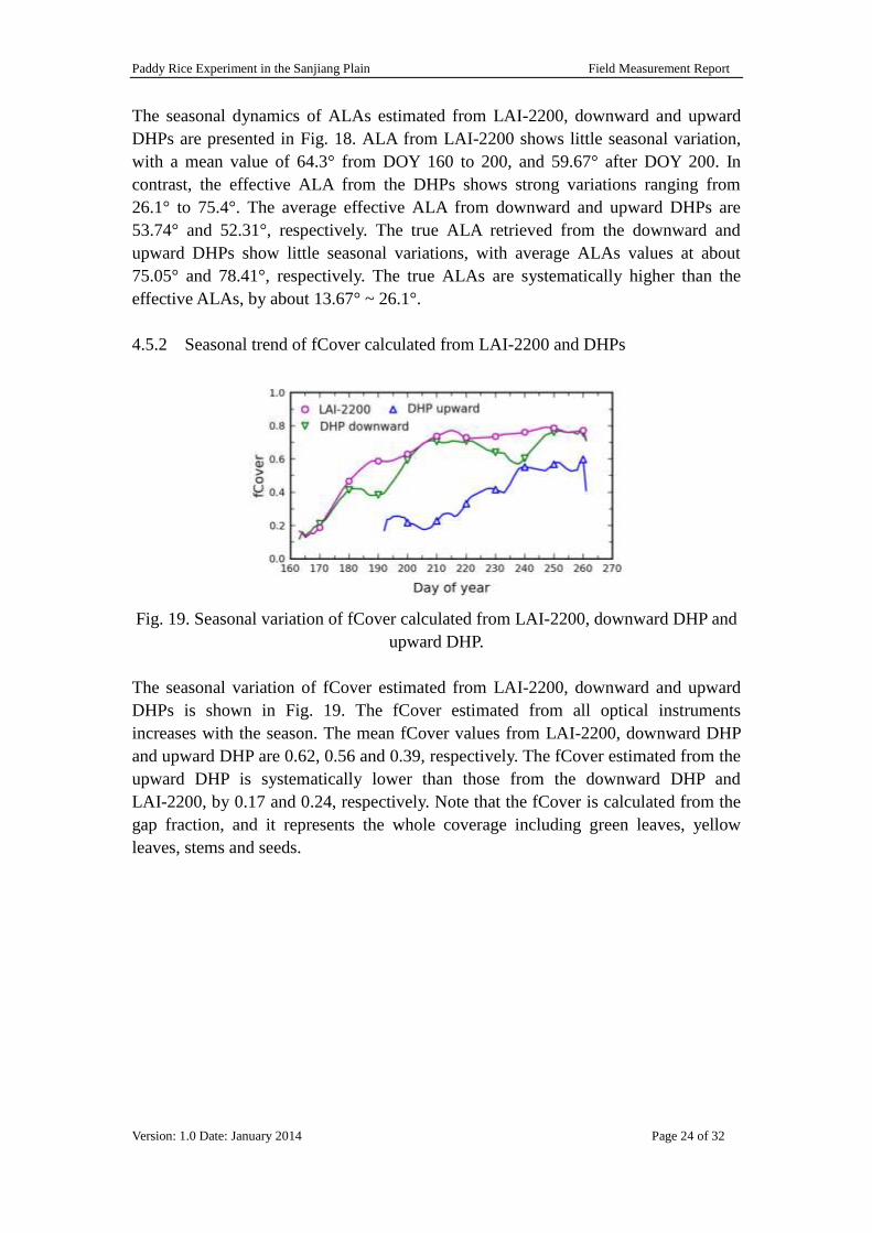
4.5.2 Seasonal trend of fCover calculated from LAI-2200 and DHPs

Fig. 19. Seasonal variation of fCover calculated from LAI-2200, downward DHP and

upward DHP.

The seasonal variation of fCover estimated from LAI-2200, downward and upward

DHPs is shown in Fig. 19. The fCover estimated from all optical instruments

increases with the season. The mean fCover values from LAI-2200, downward DHP

and upward DHP are 0.62, 0.56 and 0.39, respectively. The fCover estimated from the

upward DHP is systematically lower than those from the downward DHP and

LAI-2200, by 0.17 and 0.24, respectively. Note that the fCover is calculated from the

gap fraction, and it represents the whole coverage including green leaves, yellow

leaves, stems and seeds.



5. Quality assurance

The study area is considered homogeneous at a 3 3 km2 area. The five plots are

located away from the road, irrigation canals and ditches. The field management

practices and environmental conditions are similar for these plots. Weekly field

measurement began right after the transplantation and ended when the rice was ready

for harvest. Nearly all measurements were performed under diffuse radiation

condition, i.e., near the sunset or during overcast days.

The optical instruments were newly purchased and were tested before the field

campaign. Instrument calibrations were performed before or during the measurements,

according to the instrument manual. However, unexpected incidents have happened

during the field work and they are noted in Table 4.

For LAI-2200, the direct illumination could happen and the 270° view cap was

missing for several occasions. Measurement for Plot B on August 2 was conducted

under direct radiation with a 90° view cap and the measurements for Plot D on August

20 was also under the direct illumination condition with a 270° view cap. No view

cap was used for Plot B on September 6, for Plot C on August 22, August 28 and

September 5, and for Plot E on September 8 because the 270° view cap was missing

during the measurements. Furthermore, unreliable data with very small above-canopy

radiation readings (< 10°) were also deleted, including the measurements for Plot A

(July 31), Plot B (July 16), Plot C (August 22 and September 16), Plot D (July 30)

and Plot E (August 20).

The downward DHP photos taken over Plot A on July 11 and July 31, over Plot C on

July 18, and over Plot E on August 4 were too dark for classification and were

excluded. The upward photos taken for Plot B on August 27 were also deleted due to

the dark sky.

When the PAR value is less than 10 umol/m2s, the AccuPAR measurements were not

used. Measurements at Plots A on July 31 and at Plot E on July 10 were purged from

further analysis due to the low PAR readings.

For the destructive method, seeds collected for Plot E on July 17 were only measured

by the scanner. The LI-3100C was out of work for nearly one week (August 20 –

August 27) (Table 4). Accordingly, the bundles collected for Plot D and E on August

20 were all scanned by the scanner, with leaves sticked to white papers by tapes.

Moreover, seeds were only scanned by the scanner for Plot E on August 20. The rice

bundles for Plot A (August 24), and Plot B (August 27) were frozen in a refrigerator

and processed using the LI-3100C after it resumed working.



Table 4. Major morphological changes, rice height, water depth and instruments

conditions during the measurement.

From left to right: plot ID, measurement dates, Day of year, phenological stage (TL:

tillering, FL: flowering, GF: grain filling, MA: maturation, including yellow

maturation), average height of the plants, wetness of the soil, depth of soil water (W:

wet, WS: water saturate, WL: water logged), the sky illumination condition (Dif:

diffuse dominant, Dir: direct sunlight, Block: the direct sun was obscured by cloud

during measurements), green leaves measurements, ears appearance, yellow leaves

appearance, LAI-2200 view cap (VC) status (HM: handmade 270°), AccuPAR status,

the number of photos for the downward looking DHPs and upward looking DHPs,

and the LI3000C usability status. Symbol ‘√’ represents all data are good and

‘-‘ represents no measurements or no good data.



ID Dates DOY Pheno

.

H

(m)

Soil WD

(m)

Sky Green

leaves

Seed

Yellow

leaves

LAI-2200 AccuPAR DHP(↓) DHP(↑) LI3000C

A 2012/6/11 163 TL 0.21 WL 0.05 Dif √ - - √ √ 20 - √

A 2012/6/18 170 TL 0.32 WL 0.10 Dif √ - - √ √ 20 - √

A 2012/6/27 179 TL 0.43 WL 0.06 Dif √ - - √ √ 20 - √

A 2012/7/6 188 FL 0.62 WL 0.08 Dif √ - - √ √ 20 - √

A 2012/7/11 193 FL 0.69 WL 0.10 Dif √ √ - √ √ - 15 √

A 2012/7/20 202 FL 0.96 WL 0.06 Dif √ √ - √ √ 20 19 √

A 2012/7/26 208 FL 0.95 WL 0.06 Dif √ √ - √ √ 20 20 √

A 2012/7/31 213 FL 0.86 WL 0.10 Dif √ √ - - - - 9 √

A 2012/8/9 222 GF 0.91 WL 0.02 Dif √ √ √ √ √ 20 15 √

A 2012/8/16 229 GF 0.97 WS 0.00 Dif √ √ √ √ √ 20 18 √

A 2012/8/24 237 GF 0.91 W 0.00 Dif √ √ √ √ √ 20 20 √

A 2012/9/3 247 MA 0.88 W 0.00 Dif √ √ √ HM VC √ 20 20 √

A 2012/9/12 256 MA 1.00 WL 0.02 Dif √ √ √ √ √ 20 20 √

A 2012/9/17 261 MA 1.00 W 0.00 Dif √ √ √ √ √ 20 20 √

B 2012/6/16 168 TL 0.29 WL 0.09 Dif √ - - √ √ 20 - √

B 2012/6/20 172 TL 0.31 WL 0.10 Dif √ - - √ √ 20 - √

B 2012/6/25 177 TL 0.41 WL 0.06 Dif √ - - √ √ 20 - √

B 2012/7/2 184 TL 0.52 WL 0.03 Dif √ - - √ √ 20 - √

B 2012/7/9 191 FL 0.66 WS 0.00 Dif √ - - √ √ 20 - √

B 2012/7/16 198 FL 0.80 WS 0.00 Dif √ √ - - √ 20 15 √

B 2012/7/23 205 FL 0.81 WS 0.00 Dif √ √ - √ √ 20 10 √

B 2012/8/2 215 GF 0.95 WL 0.08 Dir √ √ - 90° VC √ 20 20 √

B 2012/8/6 219 GF 0.86 WS 0.00 Block √ √ √ √ √ 20 16 √



B 2012/8/13 226 GF 0.81 W 0.00 Dif √ √ √ √ √ 20 20 √

B 2012/8/23 236 GF 0.85 W 0.00 Dif √ √ √ √ √ 20 20 √

B 2012/8/27 240 GF 0.82 W 0.00 Dif √ √ √ 270°+NO √ 12 - √

B 2012/9/6 250 MA 0.83 WL 0.01 Dif √ √ √ No VC √ 14 20 √

B 2012/9/12 256 MA 0.91 WL 0.01 Dif √ √ √ √ √ 20 20 √

B 2012/9/16 260 MA 0.90 W 0.00 Dif √ √ √ √ √ 20 20 √

C 2012/6/13 165 TL 0.21 WL 0.14 Dif √ - - 180° VC √ 20 - √

C 2012/6/21 173 TL 0.37 WL 0.13 Dif √ - - √ √ 20 - √

C 2012/6/28 180 TL 0.46 WL 0.11 Dif √ - - √ √ 20 - √

C 2012/7/4 186 TL 0.53 WL 0.09 Dif √ - - √ √ 20 - √

C 2012/7/12 194 FL 0.78 WL 0.12 Dif √ √ - √ √ 20 - √

C 2012/7/18 200 FL 0.84 WL 0.09 Dif √ √ - √ √ - 9 √

C 2012/7/24 206 FL 0.90 WL 0.04 Dif √ √ - √ √ 8 20 √

C 2012/8/1 214 GF 0.95 WL 0.08 Dif √ √ - √ √ 20 15 √

C 2012/8/7 220 GF 0.86 WL 0.03 Dif √ √ √ √ √ 20 20 √

C 2012/8/15 228 GF 0.87 WS 0.00 Dif √ √ √ √ √ 20 20 √

C 2012/8/22 235 GF 0.93 W 0.00 Dif √ √ √ - √ 14 8 √

C 2012/8/28 241 GF 0.86 W 0.00 Dif √ √ √ No VC √ 8 11 √

C 2012/9/5 249 MA 0.88 WS 0.00 Dif √ √ √ No VC √ 17 17 √

C 2012/9/11 255 MA 0.88 W 0.00 Dif √ √ √ √ √ 20 20 √

C 2012/9/16 260 MA 0.92 W 0.00 Dif √ √ √ - √ 20 20 √

D 2012/6/12 164 TL 0.30 WL - Dif √ - - √ √ 9 - √

D 2012/6/22 174 TL 0.35 WL 0.08 Dif √ - - √ √ 20 - √

D 2012/6/29 181 TL 0.44 WL 0.11 Dif √ - - √ √ 20 - √



D 2012/7/5 187 FL 0.58 WL 0.06 Dif √ - - √ √ 20 - √

D 2012/7/13 195 FL 0.62 WL 0.10 Dif √ - - √ √ 8 9 √

D 2012/7/20 202 FL 0.75 WL 0.06 Dif √ √ - √ √ 8 8 √

D 2012/7/30 212 FL 0.77 WL 0.11 Dif √ √ - - √ 13 20 √

D 2012/8/3 216 GF 0.93 WL 0.09 Dif √ √ - √ √ 20 8 √

D 2012/8/9 222 GF 0.95 WL 0.05 Dif √ √ √ √ √ 9 15 √

D 2012/8/20 233 GF 0.87 WL 0.02 Dir √ - √ √ √ 8 17 -

D 2012/8/25 238 GF 0.88 WS 0.00 Dif √ √ √ √ √ 8 20 √

D 2012/9/3 247 MA 0.88 W 0.00 Dif √ √ √ HM VC √ 20 20 √

D 2012/9/10 254 MA 0.93 W 0.00 Dif √ √ √ No VC √ 20 20 √

D 2012/9/14 258 MA 1.00 W 0.00 Dif √ √ √ √ √ 14 20 √

√

E 2012/6/14 166 TL 0.28 WL 0.08 Dif √ - - √ √ 20 - √

E 2012/6/19 171 TL 0.42 WL 0.09 Dif √ - - √ √ 20 - √

E 2012/6/26 178 TL 0.47 WL 0.10 Dif √ - - √ √ 20 - √

E 2012/7/3 185 FL 0.66 WL 0.05 Dif √ - - √ √ 20 - √

E 2012/7/10 192 FL 0.73 WL 0.09 Dif √ √ - √ - 8 20 √

E 2012/7/17 199 FL 0.74 WL 0.12 Dif √ √ - √ √ 9 8 √

E 2012/7/23 205 FL 0.88 WL 0.08 Dif √ √ - √ √ 20 20 √

E 2012/8/4 217 GF 0.90 WL 0.09 Block √ √ √ √ √ - 15 √

E 2012/8/8 221 GF 0.89 WL 0.04 Block √ √ √ √ √ 20 20 √

E 2012/8/14 227 GF 0.93 W 0.00 Dif √ √ √ √ √ 20 10 √

E 2012/8/20 233 GF 0.94 W 0.00 Dir √ - √ - √ 13 12 -

E 2012/8/26 239 GF 0.93 W 0.00 Dif √ √ √ √ √ 20 20 √

E 2012/9/8 252 MA 0.91 W 0.00 Dif √ √ √ No VC √ 20 20 √

E 2012/9/14 258 MA 0.92 W 0.00 Dif √ √ √ √ √ 20 20 √



6. Data access and citation

6.1 Data access

All final results over each plot are provided, including PAI, PAIeff, gap fraction, CI,

ALA and fCover. They are compiled in ASCII format. Please contact the PI below for

the field measured and the processed data.

Prof. Hongliang Fang


Chinese Academy of Sciences (CAS)

11A Datun Road, Room 1318

Beijing, 100101, China

Tel: (8610) 64888055

Fax: (8610) 64889630

Email: [email protected]

6.2 Citation

Fang, H., Li, W., Wei, S., & Jiang, C. (2014). Seasonal variation of Leaf Area Index over

paddy rice fields in NE China: Intercomparison of destructive sampling, LAI-2200, digital

hemispherical photography (DHP), and AccuPAR methods. Agricultural and Forest

Meteorology, submitted.

References

mailto:[email protected]



Baret, F., Solan, B.d., Lopez-Lozano, R., Ma, K. and Weiss, M., 2010. GAI estimates of row

crops from downward looking digital photos taken perpendicular to rows at 57.5◦ zenith

angle: Theoretical considerations based on 3D architecture models and application to

wheat crops. Agricultural and Forest Meteorology, 150: 1393-1401.

Demarez, V., Duthoit, S., Baret, F., Weiss, M. and Dedieu, G., 2008. Estimation of leaf area

and clumping indexes of crops with hemispherical photographs. Agricultural and Forest

Meteorology, 148: 644-655.

Fang, H., Li, W., Wei, S. and Jiang, C., 2014. Seasonal variation of Leaf Area Index over

paddy rice fields in NE China: Intercomparison of destructive sampling, LAI-2200, digital

hemispherical photography (DHP), and AccuPAR methods. Agricultural and Forest

Meteorology, submitted.

Garrigues, S. et al., 2008. Validation and intercomparison of global Leaf Area Index products

derived from remote sensing data. Journal of Geophysical Research: Biogeosciences, 113.

Lang, A.R.G., McMurtrie, R.E. and Benson, M.L., 1991. Validity of surface area indices of

Pinus radiata estimated from transmittance of the sun's beam. Agricultural and Forest

Meteorology, 57(1–3): 157-170.

Lang, A.R.G. and Xiang, Y., 1986. Estimation of leaf area index from transmission of direct

sunlight in discontinuous canopies. Agricultural and Forest Meteorology, 37: 229-243.

Miller, J.B., 1967. A formula for average foliage density. Australian Journal of Botany, 15:

141-144.

Nilson, T., 1971. A theoretical analysis of the frequency of gaps in plant stands. Agricultural


Norman, J.M. and Welles, J.M., 1983. Radiative transfer in an array of canopies. Agronomy

Journal, 75: 481-488.

Ryu, Y. et al., 2010. On the correct estimation of effective leaf area index: Does it reveal

information on clumping effects? Agricultural and Forest Meteorology, 150: 463-472.

Song, C., Xu, X., Tian, H. and Wang, Y., 2009. Ecosystem–atmosphere exchange of CH4 and

N2O and ecosystem respiration in wetlands in the Sanjiang Plain, Northeastern China.

Global Change Biology, 15(3): 692-705.

Stenberg, P., 2006. A note on the G-function for needle leaf canopies. Agricultural and Forest


Weiss, M. and Baret, F., 2010. CAN-EYE V6.1 user manual.

Weiss, M., Baret, F., Smith, G.J., Jonckheere, I. and Coppin, P., 2004. Review of methods for

in situ leaf area index (LAI) determination Part II. Estimation of LAI, errors and sampling.

Agricultural and Forest Meteorology, 121: 37-53.

Yang, W., Hao, F., Cheng, H., Lin, C. and Ouyang, W., 2013. Phosphorus fractions and

availability in an Albic Bleached Meadow soil. Agronomy Journal, 105(5): 1451-1457.

paddy rice experiment in the sanjiang plain (presp)

Documents