•packet classification -...

From a Nick McKeown's tutorial, 1999 and slides from Kalyanaraman (with figure from Keshav) Some slides modified by C. Pham

1

• ATM and MPLS switches– Direct Lookup

• Bridges and Ethernet switches– Associative Lookup– Hashing– Trees and tries

• IP Routers– CIDR– Patricia trees/tries– Other methods– Caching

• Packet Classification


2

Direct Lookup

VCIMemory

(Port, VCI)


3






4

Associative Lookups

NetworkAddress

AssociatedData

AssociativeMemory or CAM

Search Data

48

log2N

AssociatedData

Hit?

Address{Advantages:• Simple

Disadvantages• Slow

• High Power

• Small

• Expensive


5

Hashing

HashingFunction

Memory

Add

ress

Dat

a

Search Data

48

log2N

AssociatedData

Hit?

Address{16


6

An example

Hashing Function

CRC-1616

#1 #2 #3 #4

#1 #2

#1 #2 #3Linked lists

Memory

Search Data

48

log2N

AssociatedData

Hit?

Address{M entries

N lists


7

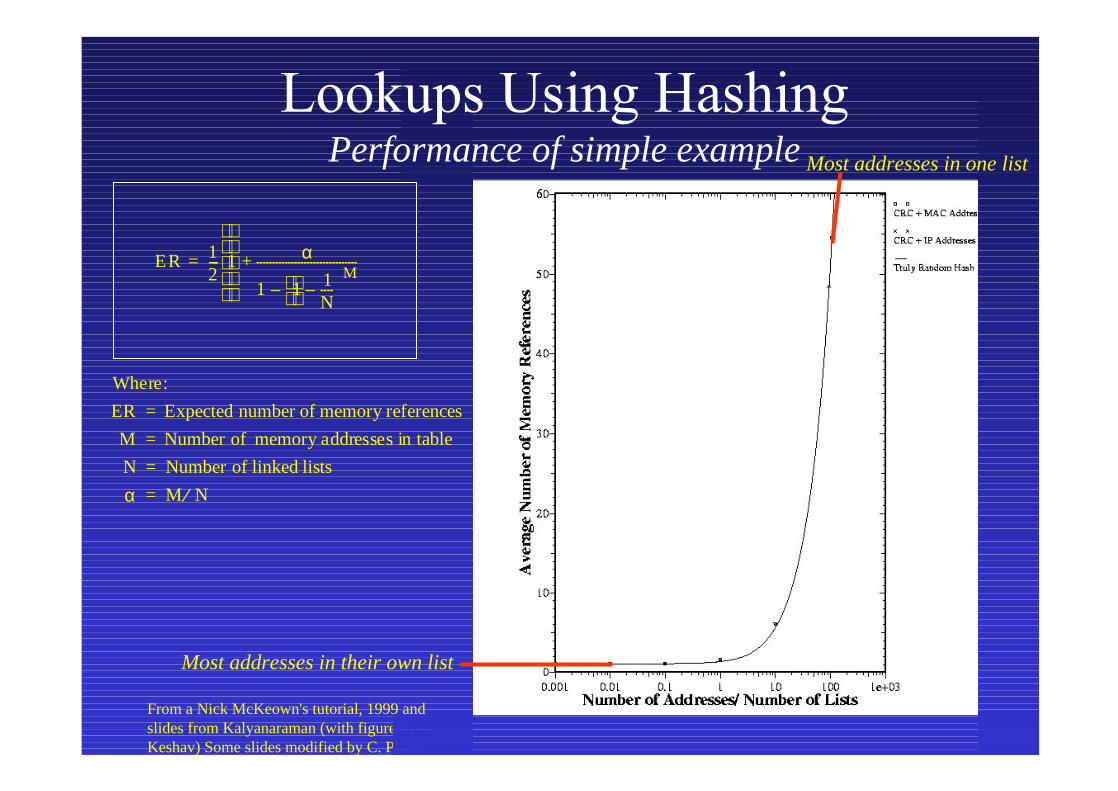
Performance of simple example

Where:

ER Expected number of memory references=

M Number of memory addresses in table=

N Number of linked lists=

α M N⁄=

ER 12--- 1 α

1 1 1N----–

M–

--------------------------------+

=

Most addresses in their own list

Most addresses in one list


8

Advantages:

• Simple

• Expected lookup time can be small

Disadvantages

• Non-deterministic lookup time

• Inefficient use of memory


9

Binary Search Tree

< >

< > < >

2

N entries

Binary Search Trie

0 1

0 1 0 1

111010


10

• An entry is:– a pointer to another array,– a special symbol indicating no

better match– a null pointer indicating that

the longst match is the parent node

• Two ways to improve performance– cache recently used addresses

in a CAM– move common entries up to a

higher level (match longer strings)

128.32.1.2 ?


11

Multiway tries

16-ary Search Trie

0000, ptr 1111, ptr

0000, 0 1111, ptr

000011110000

0000, 0 1111, ptr

111111111111


12

Multiway tries

Degree ofTree

# MemReferences

# Nodes(x106)

Total Memory(Mbytes)

FractionWasted (%)

2481664256

Ew DL 1– 1 1 N

DL-------–

D–

Di 1 Di 1––() N 1 D1 i––() N–()i 1=

L 1–

∑+=

En 1 DL 1 N

DL-------–

DDi Di 1– 1 Di 1––() N–

i 1=

L 1–

∑+ +=

Where:

D Degree of tree=

L Number of layers/references=

N Number of entries in table =

En Expected number of nodes=

Ew Expected amount of wasted memory=

Table produced from 215 randomly generated 48-bit addresses


13






14

Class-based addresses

Class A Class B Class C D

212.17.9.4

Class A

Class B

Class C212.17.9.0 Port 4

ExactMatch

Routing Table:

IP Address Space


15

CIDR

A B C D0 232-1

0 232-1

128.9/16

128.9.0.0

216

142.12/19

65/24

Classless:

Class-based:

128.9.16.14


16

CIDR

0 232-1

128.9/16

128.9.16.14

128.9.16/20 128.9.176/20

128.9.19/24

128.9.25/24

Most specific route = “longest matching prefix”


17

Metrics for Lookups

128.9/16128.9.16/20

128.9.176/20

128.9.19/24128.9.25/24

142.12/19

65/24

Prefix Port35271013

128.9.16.14

• Lookup time• Storage space• Update time• Preprocessing time


18

Lookup

IPv4 unicast destination address based lookup

Dstn Addr Next Hop

--------

---- ----

--------

Destination Next HopForwarding Table

Next Hop Computation

Forwarding Engine

Incoming Packet

HEADER


20

Gigabit Ethernet (84B packets): 1.49 Mpps

Line Line Rate Pktsize=40B Pktsize=240B

T1 1.5Mbps 4.68 Kpps 0.78 Kpps

OC3 155Mbps 480 Kpps 80 Kpps

OC12 622Mbps 1.94 Mpps 323 Kpps

OC48 2.5Gbps 7.81 Mpps 1.3 Mpps

OC192 10 Gbps 31.25 Mpps 5.21 Mpps


21

Source: http://www.telstra.net/ops/bgptable.html

Exponentialgrowth before

CIDR

About10k newprefixes per year


22

0

10000

20000

30000

40000

50000

60000

70000

80000

90000

100000

SizeSource: http://www.telstra.net/ops/bgptable.html

95 96 97 98 99 00Year

Num

ber

of

Pref

ixes

10,000/year

Renewed ExponentialGrowth

Renewed growth due to multi-homing of enterprise networks!


31

Prefix length

Most prefixes are 24-bits or shorter


32

Prefixes up to 24-bits

1 Next Hop

24

Next Hop

142.19.6

224 = 16M entries


33

Prefixes up to 24-bits

1 Next Hop

128.3.72

24 0 Pointer

8

Prefixes above 24-bits

Next Hop

Next Hop

Next Hop


36

CPU BufferMemory

LineCard

DMA

MAC

LocalBuffer

Memory

LineCard

DMA

MAC

LocalBuffer

Memory

LineCard

DMA

MAC

LocalBuffer

Memory

Fast Path

Slow Path

Advantages

Increased average lookup performance

Disadvantages

Decreased locality in backbone traffic

Cache size

Cache management overhead

Hardware implementation difficult


37

LAN:Average flow < 40 packets

WAN: Huge Number of flows

0%10%

20%30%

40%50%

60%70%

80%90%

100%

Cache = 10% of Full Table

CacheHit Rate


38

References

• A. Brodnik, S. Carlsson, M. Degermark, S. Pink. “Small Forwarding Tables for Fast Routing Lookups”, Sigcomm 1997, pp 3-14.

• B. Lampson, V. Srinivasan, G. Varghese. “ IP lookups using multiwayand multicolumn search”, Infocom 1998, pp 1248-56, vol. 3.

• M. Waldvogel, G. Varghese, J. Turner, B. Plattner. “Scalable high speed IP routing lookups”, Sigcomm 1997, pp 25-36.

• P. Gupta, S. Lin, N.McKeown. “Routing lookups in hardware at memory access speeds”, Infocom 1998, pp 1241-1248, vol. 3.

• S. Nilsson, G. Karlsson. “Fast address lookup for Internet routers”, IFIP Intl Conf on Broadband Communications, Stuttgart, Germany, April 1-3, 1998.

• V. Srinivasan, G.Varghese. “Fast IP lookups using controlled prefix expansion”, Sigmetrics, June 1998.


45

• Packet Lookup and Classification:Where does a packet go next?

• Switching Fabrics:How does the packet get there?


46

• Overview• Output and Input Queueing • Output Queueing• Input Queueing

– Scheduling algorithms– Combining input and output queues– Multicast traffic– Other non-blocking fabrics

• Multistage Switches


47

Datapath: per-packet processing

ForwardingDecision

ForwardingDecision

ForwardingDecision

ForwardingTable

ForwardingTable

ForwardingTable

Interconnect

OutputScheduling

1.

2.

3.

Transfers data from an input to an output

many ports (density), high speeds


48

• A switch that can handle N calls has N logical inputs and N logical outputs– N up to 200,000

• Moves 8-bit samples from an input to an output port– Recall that samples have no headers– Destination of sample depends on time at which it arrives at the

switch

• In practice, input trunks are multiplexed– Multiplexed trunks carry frames = set of samples

• Goal: extract samples from frame, and depending on position in frame, switch to output– each incoming sample has to get to the right output line and the

right slot in the output frame


49

• Can’t find a path from input to output

• Internal blocking– slot in output frame exists, but no path

• Output blocking– no slot in output frame is available

• Output blocking is reduced in transit switches– need to put a sample in one of several slots

going to the desired next hop


50

• Most trunks time division multiplex voice samples

• At a central office, trunk is demultiplexed and distributed to active circuits

• Synchronous multiplexor– N input lines

– Output runs N times as fast as input

…

123

N

MUX…

123

N

De-MUX1 2 3 … N


51

• Key idea: when de-multiplexing, position in frame determines output trunk

• Time division switching interchanges sample position within a frame: time slot interchange (TSI)


52

• To build a 120,000 circuit switch– read and write samples 120,000 every 125us, a

R&W operation in 0.5 ns!

– Today DRAM has access time from 80 to 40 ns

– If we use 40 ns DRAM, it's 80 times more than what we need

– Maximum #circuit= 120,000/80=1500!

– Too small!!


53

• Each sample takes a different path through the switch, depending on its destination


54

• Simplest possible space-division switch

• Crosspoints can be turned on or off, long enough to transfer a packet from an input to an output

• Expensive• Internally nonblocking

– but need N2 crosspoints– time to set each crosspoint

grows quadratically

configuration Data Out


55

• In a crossbar during each switching time only one cross-point per row or column is active

• Can save crosspoints if a cross-point can attach to more than one input line

• This is done in a multistage crossbar

N/narraysn x k

karraysN/n x N/n

N/narraywk x n


56

• Can suffer internal blocking– unless sufficient number of second-level stages,

k ≥ n

• Number of crosspoints < N2

• Finding a path from input to output requires a depth-first-search

• Scales better than crossbar, but still not too well– 120,000 call switch needs ~250 million

crosspoints


57

• In a central switching system, the high cost is the line card.

• Now the true cost is the copper wire to the customer premises!!

• In long-distance, the high cost is in laying lines, acquiring rights of way and switch-control software!

• So, saving a few thousand crosspoints is not going to make phone call cheaper!


58

• In a circuit switch, path of a sample is determined at time of connection establishment

• No need for a sample header--position in frame used

• In a packet switch, packets carry a destination field or label– Need to look up destination port on-the-fly

• Datagram switches– lookup based on entire destination address (longest-

prefix match)

• Cell or Label-switches– lookup based on VCI or Labels


59

• Can have both internal and output blocking• Internal

– no path to output

• Output– trunk unavailable

• Unlike a circuit switch, cannot predict if packets will block (why?)

• If packet is blocked, must either buffer or drop


60

• Over-provisioning– internal links much faster than inputs

• Buffers– at input or output

• Backpressure– if switch fabric doesn’t have buffers, prevent

packet from entering until path is available

• Parallel switch fabrics– increases effective switching capacity


61

• What happens if packets at two inputs both want to go to same output?

• Can defer one at an input buffer

• Or, buffer cross-points: complex arbiter


62

• Goal: towards building “self-routing” fabrics• Can build complicated fabrics from a simple

element

• Routing rule: if 0, send packet to upper output, else to lower output– If both packets to same output, buffer or drop

0

1

data 10

data 00


63

• Simplest self-routing recursive fabric, 2n output need n stages with 2n-1 components in each stage

• What if two packets both want to go to the same output→output blocking

000

001

010

011

100

101

110

111

000

001

010

011

100

101

110

111


64

• Can avoid blocking by choosing order in which packets appear at input ports

• If we can – present packets at inputs sorted by output– remove duplicates – remove gaps– precede banyan with a perfect shuffle stage– then no internal blocking

• For example: [X, 011, 010, X, 011, X, X, X]:• Sort => [010, 011, 011, X, X, X, X, X]• Remove dups => [010, 011, X, X, X, X, X, X]• Shuffle => [010, X, 011, X, X, X, X, X]• Need sort, trap and shuffle networks.


65

• Build sorters from merge networks

• Assume we can merge two sorted lists

• Sort pairwise, merge, recurse

Sort {5,7,2,3,6,2,4,5}

1/ sort 2 by 22/ merge adjacent lists

to get two 4-el lists3/ merge de two lists

with a merge network

23

47

2

5

4

6


66

• What about trapped duplicates?– recirculate to beginning

– or run output of trap to multiple banyans (dilation)


67

3

7

5

2

6

0

1

4

7

2

3

5

6

1

0

4

7

5

2

3

1

0

6

4

7

0

5

1

3

4

2

6

7

4

5

6

0

3

1

2

7

6

4

5

3

2

0

2

7

6

5

4

3

2

1

0

000001

010011

100101

110111

Batcher Sorter Self-Routing Network

• Fabric can be used as scheduler. •Batcher-Banyan network is blocking for multicast.

a dans le sens de la flèche si a > b,a dans le sens opposé si a est tout seul


68

Two basic queueing techniques

Input Queueing Output Queueing

Usually a non-blockingswitch fabric (e.g. crossbar)

Usually a fast bus


69

Output Queueing

Individual Output Queues Centralized Shared Memory

Memory b/w = (N+1).R

1

2

N

Memory b/w = 2N.R

1

2

N


70

The “ideal”

1

1

1

1

1

1

1

1

1

11

1

2

2

2

2

2

2


71

How fast can we make centralized shared memory?

SharedMemory

200 byte bus

5ns SRAM

1

2

N

• 5ns per memory operation• Two memory operations per packet• Therefore, up to 160Gb/s• In practice, closer to 80Gb/s


72

• Output and Input Queueing

• Output Queueing

• Input Queueing– Scheduling algorithms

– Combining input and output queues

– Multicast traffic

– Other non-blocking fabrics

• Multistage Switches


73

Input Queueing with Crossbar

configuration Data Out

Scheduler

Memory b/w = 2R


74

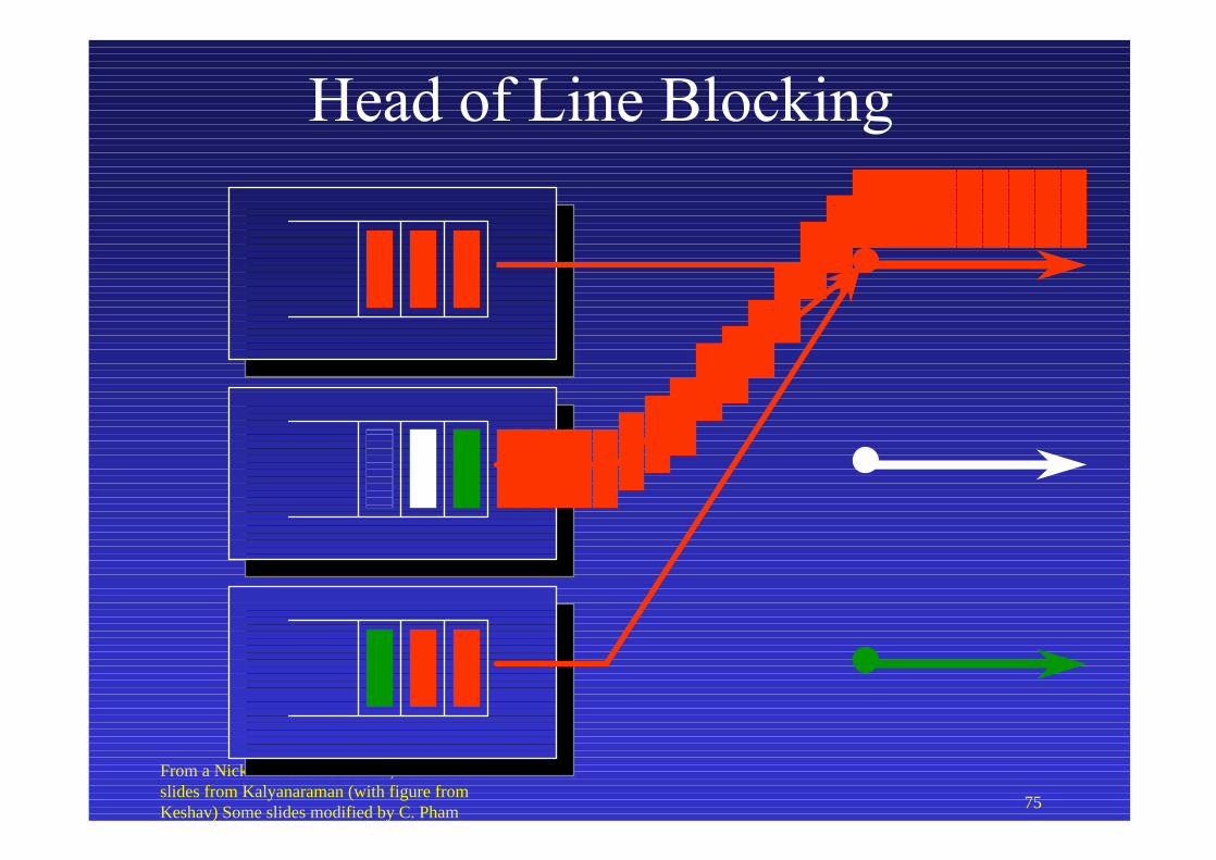
Head of Line Blocking

Del

ay

Load58.6% 100%


75


76


77


78

Virtual output queues


79

Virtual Output Queues

Del

ay

Load100%


80

Virtual Output Queues

Scheduler

Memory b/w = 2R

Can be quitecomplex!


85

Why is serving long/old queues better than serving maximum number of queues?

• When traffic is uniformly distributed, servicing themaximum number of queues leads to 100% throughput.• When traffic is non-uniform, some queues become longer than others.• A good algorithm keeps the queue lengths matched, and services a large number of queues.

VOQ #

Avg

Occ

upan

cy Uniform traffic

VOQ #

Avg

Occ

upan

cy

Non-uniform traffic


103

Shared Memory

InputQueued

Combined Input and

Output QueuedParallelPacket

Switches37526014

72356104

75231064

70513426

74560312

76453202

76543210

000001

010011

100101

110111

Batcher Sorter Self-Routing Network

Multistage

This document was created with Win2PDF available at http://www.daneprairie.com.The unregistered version of Win2PDF is for evaluation or non-commercial use only.

http://www.daneprairie.com

•packet classification -...

Documents