package ‘solar’ - the comprehensive r archive network ‘solar’ august 29, 2016 type package...

Package ‘solaR’August 29, 2016

Type Package

Title Radiation and Photovoltaic Systems

Version 0.44

Date 2016-04-16

Encoding UTF-8

Author Oscar Perpiñán Lamigueiro

Maintainer Oscar Perpiñán Lamigueiro <[email protected]>

Description Calculation methods of solar radiation and performance of photovoltaic sys-tems from daily and intradaily irradiation data sources.

URL http://oscarperpinan.github.io/solar/

BugReports https://github.com/oscarperpinan/solar/issues

License GPL-3

LazyData yes

Depends R (>= 2.10), zoo, lattice, latticeExtra

Imports RColorBrewer, graphics, grDevices, stats, methods

Suggests sp, raster, rasterVis, tdr, meteoForecast

NeedsCompilation no

Repository CRAN

Date/Publication 2016-04-16 19:49:10

R topics documented:solaR-package . . . . . . . . . . . . . . . . . . . . . . . . . . . . . . . . . . . . . . . . 3A1_calcSol . . . . . . . . . . . . . . . . . . . . . . . . . . . . . . . . . . . . . . . . . 5A2_calcG0 . . . . . . . . . . . . . . . . . . . . . . . . . . . . . . . . . . . . . . . . . 7A3_calcGef . . . . . . . . . . . . . . . . . . . . . . . . . . . . . . . . . . . . . . . . . 10A4_prodGCPV . . . . . . . . . . . . . . . . . . . . . . . . . . . . . . . . . . . . . . . 13A5_prodPVPS . . . . . . . . . . . . . . . . . . . . . . . . . . . . . . . . . . . . . . . . 17A6_calcShd . . . . . . . . . . . . . . . . . . . . . . . . . . . . . . . . . . . . . . . . . 19

1

http://oscarperpinan.github.io/solar/

https://github.com/oscarperpinan/solar/issues

2 R topics documented:

A7_optimShd . . . . . . . . . . . . . . . . . . . . . . . . . . . . . . . . . . . . . . . . 21A8_readBD . . . . . . . . . . . . . . . . . . . . . . . . . . . . . . . . . . . . . . . . . 25A8_readG0dm . . . . . . . . . . . . . . . . . . . . . . . . . . . . . . . . . . . . . . . . 27B1_Meteo-class . . . . . . . . . . . . . . . . . . . . . . . . . . . . . . . . . . . . . . . 28B2_Sol-class . . . . . . . . . . . . . . . . . . . . . . . . . . . . . . . . . . . . . . . . 29B3_G0-class . . . . . . . . . . . . . . . . . . . . . . . . . . . . . . . . . . . . . . . . . 30B4_Gef-class . . . . . . . . . . . . . . . . . . . . . . . . . . . . . . . . . . . . . . . . 31B5_ProdGCPV-class . . . . . . . . . . . . . . . . . . . . . . . . . . . . . . . . . . . . 33B6_ProdPVPS-class . . . . . . . . . . . . . . . . . . . . . . . . . . . . . . . . . . . . 35B7_Shade-class . . . . . . . . . . . . . . . . . . . . . . . . . . . . . . . . . . . . . . . 37C_corrFdKt . . . . . . . . . . . . . . . . . . . . . . . . . . . . . . . . . . . . . . . . . 38C_fBTd . . . . . . . . . . . . . . . . . . . . . . . . . . . . . . . . . . . . . . . . . . . 39C_fCompD . . . . . . . . . . . . . . . . . . . . . . . . . . . . . . . . . . . . . . . . . 41C_fCompI . . . . . . . . . . . . . . . . . . . . . . . . . . . . . . . . . . . . . . . . . . 42C_fInclin . . . . . . . . . . . . . . . . . . . . . . . . . . . . . . . . . . . . . . . . . . 44C_fProd . . . . . . . . . . . . . . . . . . . . . . . . . . . . . . . . . . . . . . . . . . . 46C_fPump . . . . . . . . . . . . . . . . . . . . . . . . . . . . . . . . . . . . . . . . . . 49C_fSolD . . . . . . . . . . . . . . . . . . . . . . . . . . . . . . . . . . . . . . . . . . . 50C_fSolI . . . . . . . . . . . . . . . . . . . . . . . . . . . . . . . . . . . . . . . . . . . 52C_fSombra . . . . . . . . . . . . . . . . . . . . . . . . . . . . . . . . . . . . . . . . . 54C_fTemp . . . . . . . . . . . . . . . . . . . . . . . . . . . . . . . . . . . . . . . . . . 57C_fTheta . . . . . . . . . . . . . . . . . . . . . . . . . . . . . . . . . . . . . . . . . . 58C_HQCurve . . . . . . . . . . . . . . . . . . . . . . . . . . . . . . . . . . . . . . . . . 59C_local2Solar . . . . . . . . . . . . . . . . . . . . . . . . . . . . . . . . . . . . . . . . 60C_NmgPVPS . . . . . . . . . . . . . . . . . . . . . . . . . . . . . . . . . . . . . . . . 62C_sample2Diff . . . . . . . . . . . . . . . . . . . . . . . . . . . . . . . . . . . . . . . 64C_utils-angle . . . . . . . . . . . . . . . . . . . . . . . . . . . . . . . . . . . . . . . . 65C_utils-time . . . . . . . . . . . . . . . . . . . . . . . . . . . . . . . . . . . . . . . . . 66D_as.data.frameD-methods . . . . . . . . . . . . . . . . . . . . . . . . . . . . . . . . . 67D_as.data.frameI-methods . . . . . . . . . . . . . . . . . . . . . . . . . . . . . . . . . 68D_as.data.frameM-methods . . . . . . . . . . . . . . . . . . . . . . . . . . . . . . . . . 68D_as.data.frameY-methods . . . . . . . . . . . . . . . . . . . . . . . . . . . . . . . . . 69D_as.zooD-methods . . . . . . . . . . . . . . . . . . . . . . . . . . . . . . . . . . . . . 70D_as.zooI-methods . . . . . . . . . . . . . . . . . . . . . . . . . . . . . . . . . . . . . 71D_as.zooM-methods . . . . . . . . . . . . . . . . . . . . . . . . . . . . . . . . . . . . 72D_as.zooY-methods . . . . . . . . . . . . . . . . . . . . . . . . . . . . . . . . . . . . . 72D_compare-methods . . . . . . . . . . . . . . . . . . . . . . . . . . . . . . . . . . . . 73D_getData-methods . . . . . . . . . . . . . . . . . . . . . . . . . . . . . . . . . . . . . 74D_getG0-methods . . . . . . . . . . . . . . . . . . . . . . . . . . . . . . . . . . . . . . 75D_getLat-methods . . . . . . . . . . . . . . . . . . . . . . . . . . . . . . . . . . . . . 75D_indexD-methods . . . . . . . . . . . . . . . . . . . . . . . . . . . . . . . . . . . . . 76D_indexI-methods . . . . . . . . . . . . . . . . . . . . . . . . . . . . . . . . . . . . . 76D_indexRep-methods . . . . . . . . . . . . . . . . . . . . . . . . . . . . . . . . . . . . 76D_levelplot-methods . . . . . . . . . . . . . . . . . . . . . . . . . . . . . . . . . . . . 77D_Losses-methods . . . . . . . . . . . . . . . . . . . . . . . . . . . . . . . . . . . . . 77D_mergesolaR-methods . . . . . . . . . . . . . . . . . . . . . . . . . . . . . . . . . . 78D_shadeplot-methods . . . . . . . . . . . . . . . . . . . . . . . . . . . . . . . . . . . . 79D_window-methods . . . . . . . . . . . . . . . . . . . . . . . . . . . . . . . . . . . . . 80

solaR-package 3

D_writeSolar-methods . . . . . . . . . . . . . . . . . . . . . . . . . . . . . . . . . . . 81D_xyplot-methods . . . . . . . . . . . . . . . . . . . . . . . . . . . . . . . . . . . . . 82E_aguiar . . . . . . . . . . . . . . . . . . . . . . . . . . . . . . . . . . . . . . . . . . . 83E_helios . . . . . . . . . . . . . . . . . . . . . . . . . . . . . . . . . . . . . . . . . . . 84E_prodEx . . . . . . . . . . . . . . . . . . . . . . . . . . . . . . . . . . . . . . . . . . 84E_pumpCoef . . . . . . . . . . . . . . . . . . . . . . . . . . . . . . . . . . . . . . . . 85E_solaR.theme . . . . . . . . . . . . . . . . . . . . . . . . . . . . . . . . . . . . . . . 86solaR-defunct . . . . . . . . . . . . . . . . . . . . . . . . . . . . . . . . . . . . . . . . 86

Index 87

solaR-package Solar Radiation and Photovoltaic Systems with R

Description

The solaR package allows for reproducible research both for photovoltaics (PV) systems perfor-mance and solar radiation. It includes a set of classes, methods and functions to calculate the sungeometry and the solar radiation incident on a photovoltaic generator and to simulate the perfor-mance of several applications of the photovoltaic energy. This package performs the whole calcula-tion procedure from both daily and intradaily global horizontal irradiation to the final productivityof grid-connected PV systems and water pumping PV systems.

Details

solaR is designed using a set of S4 classes whose core is a group of slots with multivariate timeseries. The classes share a variety of methods to access the information and several visualizationmethods. In addition, the package provides a tool for the visual statistical analysis of the perfor-mance of a large PV plant composed of several systems.

Although solaR is primarily designed for time series associated to a location defined by its lat-itude/longitude values and the temperature and irradiation conditions, it can be easily combinedwith spatial packages for space-time analysis.

The best place to learn how to use the package is the companion paper published by the Journal ofStatistical Software: http://www.jstatsoft.org/v50/i09/

Please note that this package needs to set the timezone to UTC. Every ‘zoo’ object created bythe package will have an index with this time zone as a synonym of mean solar time..You can check it after loading solaR with:

Sys.getenv('TZ')

If you need to change it, use:

Sys.setenv(TZ = 'YourTimeZone')

Index of functions and classes:

G0-class Class "G0": irradiation and irradiance on thehorizontal plane.

Gef-class Class "Gef": irradiation and irradiance on the

4 solaR-package

generator plane.HQCurve H-Q curves of a centrifugal pumpMeteo-class Class "Meteo"NmgPVPS Nomogram of a photovoltaic pumping systemProdGCPV-class Class "ProdGCPV": performance of a grid

connected PV system.ProdPVPS-class Class "ProdPVPS": performance of a PV pumping

system.Shade-class Class "Shade": shadows in a PV system.Sol-class Class "Sol": Apparent movement of the Sun from

the Earthaguiar Markov Transition Matrices for the Aguiar etal.

procedureas.data.frameD Methods for Function as.data.frameDas.data.frameI Methods for Function as.data.frameIas.data.frameM Methods for Function as.data.frameMas.data.frameY Methods for Function as.data.frameYas.zooD Methods for Function as.zooDas.zooI-methods Methods for Function as.zooIas.zooM Methods for Function as.zooMas.zooY Methods for Function as.zooYcalcG0 Irradiation and irradiance on the horizontal

plane.calcGef Irradiation and irradiance on the generator

plane.calcShd Shadows on PV systems.calcSol Apparent movement of the Sun from the Earthcompare Compare G0, Gef and ProdGCPV objectscompareLosses Losses of a GCPV systemcorrFdKt Correlations between the fraction of diffuse

irradiation and the clearness index.d2r Conversion between angle units.diff2Hours Small utilities for difftime objects.fBTd Daily time basefCompD Components of daily global solar irradiation on

a horizontal surfacefCompI Calculation of solar irradiance on a horizontal

surfacefInclin Solar irradiance on an inclined surfacefProd Performance of a PV systemfPump Performance of a centrifugal pumpfSolD Daily apparent movement of the Sun from the

EarthfSolI Instantaneous apparent movement of the Sun from

the EarthfSombra Shadows on PV systemsfTemp Intradaily evolution of ambient temperaturefTheta Angle of incidence of solar irradiation on a

A1_calcSol 5

inclined surfacegetData Methods for function getDatagetG0 Methods for function getG0getLat Methods for Function getLathelios Daily irradiation and ambient temperature from

the Helios-IES databasehour Utilities for time indexes.indexD Methods for Function indexDindexI Methods for Function indexIindexRep-methods Methods for Function indexReplevelplot-methods Methods for function levelplot.local2Solar Local time, mean solar time and UTC time zone.mergesolaR Merge solaR objectsoptimShd Shadows calculation for a set of distances

between elements of a PV grid connected plant.prodEx Productivity of a set of PV systems of a PV

plant.prodGCPV Performance of a grid connected PV system.prodPVPS Performance of a PV pumping systempumpCoef Coefficients of centrifugal pumps.readBD Daily or intradaily values of global horizontal

irradiation and ambient temperature from alocal file or a data.frame.

readG0dm Monthly mean values of global horizontalirradiation.

shadeplot Methods for Function shadeplotsolaR.theme solaR themewindow Methods for extracting a time windowwriteSolar Exporter of solaR resultsxyplot-methods Methods for function xyplot in Package 'solaR'

Author(s)

Oscar Perpiñán Lamigueiro

Maintainer: Oscar Perpiñán Lamigueiro <[email protected]>

A1_calcSol Apparent movement of the Sun from the Earth

Description

Compute the apparent movement of the Sun from the Earth with the functions fSolD and fSolI.

Usage

calcSol(lat, BTd, sample='hour', BTi, EoT=TRUE, keep.night=TRUE, method='michalsky')

6 A1_calcSol

Arguments

lat Latitude (degrees) of the point of the Earth where calculations are needed. It ispositive for locations above the Equator.

BTd Daily time base, a POSIXct object which may be the result of fBTd. It is notconsidered if BTi is provided.

sample Increment of the intradaily sequence. It is a character string, containing oneof ‘"sec"’, ‘"min"’, ‘"hour"’. This can optionally be preceded by a (positive ornegative) integer and a space, or followed by ‘"s"’. It is used by seq.POSIXt.It is not considered if BTi is provided.

BTi Intradaily time base, a POSIXct object to be used by fSolI. It could be the indexof the G0I argument to calcG0.

EoT logical, if TRUE the Equation of Time is used. Default is TRUE.

keep.night logical, if TRUE (default) the night is included in the time series.

method character, method for the sun geometry calculations to be chosen from ’cooper’,’spencer’, ’michalsky’ and ’strous’. See references for details.

Value

A Sol-class object.

Author(s)

Oscar Perpiñán Lamigueiro.

References

• Cooper, P.I., Solar Energy, 12, 3 (1969). "The Absorption of Solar Radiation in Solar Stills"

• Spencer, Search 2 (5), 172, http://www.mail-archive.com/[email protected]/msg01050.html

• Strous: http://aa.quae.nl/en/reken/zonpositie.html

• Michalsky, J., 1988: The Astronomical Almanac’s algorithm for approximate solar position(1950-2050), Solar Energy 40, 227-235

• Perpiñán, O, Energía Solar Fotovoltaica, 2015. (http://oscarperpinan.github.io/esf/)

• Perpiñán, O. (2012), "solaR: Solar Radiation and Photovoltaic Systems with R", Journal ofStatistical Software, 50(9), 1-32, http://www.jstatsoft.org/v50/i09/

Examples

BTd=fBTd(mode='serie')

lat=37.2sol=calcSol(lat, BTd[100])print(as.zooD(sol))

library(lattice)xyplot(as.zooI(sol))

http://www.mail-archive.com/[email protected]/msg01050.html


http://aa.quae.nl/en/reken/zonpositie.html

http://oscarperpinan.github.io/esf/

http://www.jstatsoft.org/v50/i09/

A2_calcG0 7

solStrous=calcSol(lat, BTd[100], method='strous')print(as.zooD(solStrous))

solSpencer=calcSol(lat, BTd[100], method='spencer')print(as.zooD(solSpencer))

solCooper=calcSol(lat, BTd[100], method='cooper')print(as.zooD(solCooper))

A2_calcG0 Irradiation and irradiance on the horizontal plane.

Description

This function obtains the global, diffuse and direct irradiation and irradiance on the horizontal planefrom the values of daily and intradaily global irradiation on the horizontal plane. It makes use ofthe functions calcSol, fCompD, fCompI, fBTd and readBD (or equivalent).

Besides, if information about maximum and minimum temperatures values are available it obtainsa series of temperature values with fTemp.

Usage

calcG0(lat, modeRad='prom', dataRad,sample='hour', keep.night=TRUE,sunGeometry='michalsky',corr, f, ...)

Arguments

lat numeric, latitude (degrees) of the point of the Earth where calculations areneeded. It is positive for locations above the Equator.

modeRad A character string, describes the kind of source data of the global irradiation andambient temperature.It can be modeRad='prom' for monthly mean calculations. With this option, aset of 12 values inside dataRad must be provided, as defined in readG0dm.modeRad='aguiar' uses a set of 12 monthly average values (provided withdataRad) and produces a synthetic daily irradiation time series following theprocedure by Aguiar etal. (see reference below).If modeRad='bd' the information of daily irradiation is read from a file, a data.framedefined by dataRad, a zoo or a Meteo object. (See readBD, df2Meteo andzoo2Meteo for details).If modeRad='bdI' the information of intradaily irradiation is read from a file,a data.frame defined by dataRad, a zoo or a Meteo object. (See readBDi,dfI2Meteo and zoo2Meteo for details).

8 A2_calcG0

dataRad • If modeRad='prom' or modeRad='aguiar', a numeric with 12 values or anamed list whose components will be processed with readG0dm.

• If modeRad='bd' a character (name of the file to be read with readBD), adata.frame (to be processed with df2Meteo), a zoo (to be processed withzoo2Meteo), a Meteo object, or a list as defined by readBD, df2Meteoor zoo2Meteo. The resulting object will include a column named Ta, withinformation about ambient temperature.

• If modeRad='bdI' a character (name of the file to be read with readBDi), adata.frame (to be processed with dfI2Meteo), a zoo (to be processed withzoo2Meteo), a Meteo object, or a list as defined by readBDi, dfI2Meteoor zoo2Meteo. The resulting object will include a column named Ta, withinformation about ambient temperature.

sample character, containing one of ‘"sec"’, ‘"min"’, ‘"hour"’. This can optionally bepreceded by a (positive or negative) integer and a space, or followed by ‘"s"’(used by seq.POSIXt). It is not used when modeRad="bdI".

keep.night logical. When it is TRUE (default) the time series includes the night.

sunGeometry character, method for the sun geometry calculations. See calcSol, fSolD andfSolI.

corr A character, the correlation between the the fraction of diffuse irradiation andthe clearness index to be used.With this version several options are available, as described in corrFdKt. Forexample, the FdKtPage is selected with corr='Page' while the FdKtCPR withcorr='CPR'.If corr='user' the use of a correlation defined by a function f is possible.If corr='none' the object defined by dataRad should include information aboutglobal, diffuse and direct daily irradiation with columns named G0d, D0d andB0d, respectively (or G0, D0 and B0 if modeRad='bdI'). If corr is missing, thenit is internally set to CPR when modeRad='bd', to Page when modeRad='prom'and to BRL when modeRad='bdI'.

f A function defininig a correlation between the fraction of diffuse irradiation andthe clearness index. It is only neccessary when corr='user'

... Additional arguments for fCompD or fCompI

Value

A G0 object.

Author(s)


References





A2_calcG0 9

• Aguiar, Collares-Pereira and Conde, "Simple procedure for generating sequences of dailyradiation values using a library of Markov transition matrices", Solar Energy, Volume 40,Issue 3, 1988, Pages 269–279

See Also

calcSol, fCompD, fCompI, readG0dm, readBD, readBDi, corrFdKt.

Examples

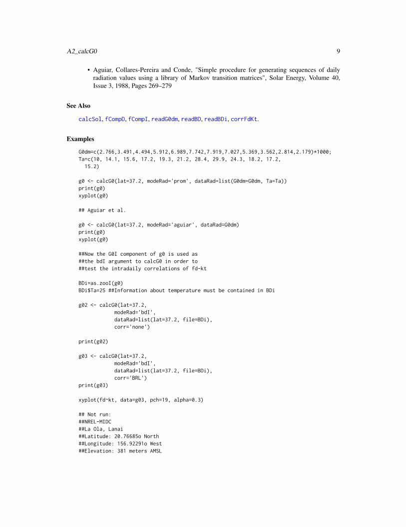
G0dm=c(2.766,3.491,4.494,5.912,6.989,7.742,7.919,7.027,5.369,3.562,2.814,2.179)*1000;Ta=c(10, 14.1, 15.6, 17.2, 19.3, 21.2, 28.4, 29.9, 24.3, 18.2, 17.2,

15.2)

g0 <- calcG0(lat=37.2, modeRad='prom', dataRad=list(G0dm=G0dm, Ta=Ta))print(g0)xyplot(g0)

## Aguiar et al.

g0 <- calcG0(lat=37.2, modeRad='aguiar', dataRad=G0dm)print(g0)xyplot(g0)

##Now the G0I component of g0 is used as##the bdI argument to calcG0 in order to##test the intradaily correlations of fd-kt

BDi=as.zooI(g0)BDi$Ta=25 ##Information about temperature must be contained in BDi

g02 <- calcG0(lat=37.2,modeRad='bdI',dataRad=list(lat=37.2, file=BDi),corr='none')

print(g02)

g03 <- calcG0(lat=37.2,modeRad='bdI',dataRad=list(lat=37.2, file=BDi),corr='BRL')

print(g03)

xyplot(fd~kt, data=g03, pch=19, alpha=0.3)

## Not run:##NREL-MIDC##La Ola, Lanai##Latitude: 20.76685o North##Longitude: 156.92291o West##Elevation: 381 meters AMSL

10 A3_calcGef

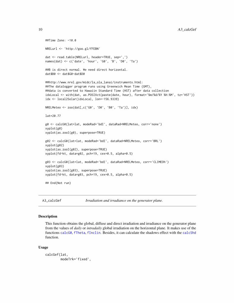
##Time Zone: -10.0

NRELurl <- 'http://goo.gl/fFEBN'

dat <- read.table(NRELurl, header=TRUE, sep=',')names(dat) <- c('date', 'hour', 'G0', 'B', 'D0', 'Ta')

##B is direct normal. We need direct horizontal.dat$B0 <- dat$G0-dat$D0

##http://www.nrel.gov/midc/la_ola_lanai/instruments.html:##The datalogger program runs using Greenwich Mean Time (GMT),##data is converted to Hawaiin Standard Time (HST) after data collectionidxLocal <- with(dat, as.POSIXct(paste(date, hour), format='%m/%d/%Y %H:%M', tz='HST'))idx <- local2Solar(idxLocal, lon=-156.9339)

NRELMeteo <- zoo(dat[,c('G0', 'D0', 'B0', 'Ta')], idx)

lat=20.77

g0 <- calcG0(lat=lat, modeRad='bdI', dataRad=NRELMeteo, corr='none')xyplot(g0)xyplot(as.zooI(g0), superpose=TRUE)

g02 <- calcG0(lat=lat, modeRad='bdI', dataRad=NRELMeteo, corr='BRL')xyplot(g02)xyplot(as.zooI(g02), superpose=TRUE)xyplot(fd~kt, data=g02, pch=19, cex=0.5, alpha=0.5)

g03 <- calcG0(lat=lat, modeRad='bdI', dataRad=NRELMeteo, corr='CLIMEDh')xyplot(g03)xyplot(as.zooI(g03), superpose=TRUE)xyplot(fd~kt, data=g03, pch=19, cex=0.5, alpha=0.5)

## End(Not run)

A3_calcGef Irradiation and irradiance on the generator plane.

Description

This function obtains the global, diffuse and direct irradiation and irradiance on the generator planefrom the values of daily or intradaily global irradiation on the horizontal plane. It makes use of thefunctions calcG0, fTheta, fInclin. Besides, it can calculate the shadows effect with the calcShdfunction.

Usage

calcGef(lat,modeTrk='fixed',

A3_calcGef 11

modeRad='prom',dataRad,sample='hour',keep.night=TRUE,sunGeometry='michalsky',corr, f,betaLim=90, beta=abs(lat)-10, alfa=0,iS=2, alb=0.2, horizBright=TRUE, HCPV=FALSE,modeShd='',struct=list(),distances=data.frame(),...)

Arguments


modeTrk character, to be chosen from 'fixed', 'two' or 'horiz'. When modeTrk='fixed'the surface is fixed (inclination and azimuth angles are constant). The perfor-mance of a two-axis tracker is calculated with modeTrk='two', and modeTrk='horiz'is the option for an horizontal N-S tracker. Its default value is modeTrk='fixed'

modeRad, dataRad

Information about the source data of the global irradiation. See calcG0 fordetails.

sample, keep.night

See calcSol for details.sunGeometry character, method for the sun geometry calculations. See calcSol, fSolD and

fSolI.corr, f See calcG0 for details.beta numeric, inclination angle of the surface (degrees). It is only needed when

modeTrk='fixed'.betaLim numeric, maximum value of the inclination angle for a tracking surface. Its

default value is 90 (no limitation))alfa numeric, azimuth angle of the surface (degrees). It is measured from the south

(alfa = 0), and it is negative to the east and positive to the west. It is onlyneeded when modeTrk='fixed'. Its default value is alfa=0

iS integer, degree of dirtiness. Its value must be included in the set (1,2,3,4). iS=1corresponds to a clean surface while iS=4 is the selection for a dirty surface. Itsdefault value is 2.

alb numeric, albedo reflection coefficient. Its default value is 0.2modeShd, struct, distances

See calcShd for details.horizBright logical, if TRUE, the horizon brightness correction proposed by Reind et al. is

used.HCPV logical, if TRUE the diffuse and albedo components of the effective irradiance

are set to zero. HCPV is the acronym of High Concentration PV system.... Additional arguments for calcSol and calcG0

12 A3_calcGef

Value

A Gef object.

Author(s)


References

• Hay, J. E. and McKay, D. C.: Estimating Solar Irradiance on Inclined Surfaces: A Review andAssessment of Methodologies. Int. J. Solar Energy, (3):pp. 203, 1985.

• Martin, N. and Ruiz, J.M.: Calculation of the PV modules angular losses under field conditionsby means of an analytical model. Solar Energy Materials & Solar Cells, 70:25–38, 2001.

• D. T. Reindl and W. A. Beckman and J. A. Duffie: Evaluation of hourly tilted surface radiationmodels, Solar Energy, 45:9-17, 1990.



See Also

calcG0, fTheta, fInclin, calcShd.

Examples

###12 Average days.

G0dm=c(2.766,3.491,4.494,5.912,6.989,7.742,7.919,7.027,5.369,3.562,2.814,2.179)*1000;Ta=c(10, 14.1, 15.6, 17.2, 19.3, 21.2, 28.4, 29.9, 24.3, 18.2, 17.2, 15.2)

##Fixed surface, default values of inclination and azimuth.

gef<-calcGef(lat=37.2, modeRad='prom', dataRad=list(G0dm=G0dm, Ta=Ta))print(gef)xyplot(gef)

##Two-axis surface, no limitation angle.

gef2<-calcGef(lat=37.2, modeRad='prom', dataRad=list(G0dm=G0dm, Ta=Ta), modeTrk='two')print(gef2)xyplot(gef2)

##Fixed surfacegefAguiar <- calcGef(lat=41, modeRad='aguiar', dataRad=G0dm)

##Two-axis tracker, using the previous result.##'gefAguiar' is internally coerced to a 'G0' object.

gefAguiar2 <- calcGef(lat=41, modeRad='prev', dataRad=gefAguiar, modeTrk='two')print(gefAguiar2)



A4_prodGCPV 13

xyplot(gefAguiar2)

###Shadows between two-axis trackers, again using the gefAguiar result.

struct=list(W=23.11, L=9.8, Nrow=2, Ncol=8)distances=data.frame(Lew=40, Lns=30, H=0)

gefShd<-calcGef(lat=41, modeRad='prev',dataRad=gefAguiar, modeTrk='two',modeShd=c('area', 'prom'),struct=struct, distances=distances)

print(gefShd)##The Gef0, Bef0 and Def0 values are the same as those contained in the## gefAguiar2 object

A4_prodGCPV Performance of a grid connected PV system.

Description

Compute every step from solar angles to effective irradiance to calculate the performance of a gridconnected PV system.

Usage

prodGCPV(lat,modeTrk='fixed',modeRad='prom',dataRad,sample='hour',keep.night=TRUE,sunGeometry='michalsky',corr, f,betaLim=90, beta=abs(lat)-10, alfa=0,iS=2, alb=0.2, horizBright=TRUE, HCPV=FALSE,module=list(),generator=list(),inverter=list(),effSys=list(),modeShd='',struct=list(),distances=data.frame(),...)

Arguments


14 A4_prodGCPV

modeTrk A character string, describing the tracking method of the generator. See calcGeffor details.

modeRad, dataRad


sample, keep.night

See calcSol for details.


corr, f See calcG0 for details.betaLim, beta, alfa, iS, alb, horizBright, HCPV

See calcGef for details.

module list of numeric values with information about the PV module,

Vocn open-circuit voltage of the module at Standard Test Conditions (defaultvalue 57.6 volts.)

Iscn short circuit current of the module at Standard Test Conditions (defaultvalue 4.7 amperes.)

Vmn maximum power point voltage of the module at Standard Test Conditions(default value 46.08 amperes.)

Imn Maximum power current of the module at Standard Test Conditions (de-fault value 4.35 amperes.)

Ncs number of cells in series inside the module (default value 96)Ncp number of cells in parallel inside the module (default value 1)CoefVT coefficient of decrement of voltage of each cell with the temperature

(default value 0.0023 volts per celsius degree)TONC nominal operational cell temperature, celsius degree (default value 47).

generator list of numeric values with information about the generator,

Nms number of modules in series (default value 12)Nmp number of modules in parallel (default value 11)

inverter list of numeric values with information about the DC/AC inverter,

Ki vector of three values, coefficients of the efficiency curve of the inverter(default c(0.01, 0.025, 0.05)), or a matrix of nine values (3x3) if there isdependence with the voltage (see references).

Pinv nominal inverter power (W) (default value 25000 watts.)Vmin, Vmax minimum and maximum voltages of the MPP range of the inverter

(default values 420 and 750 volts)Gumb minimum irradiance for the inverter to start (W/m²) (default value 20

W/m²)

effSys list of numeric values with information about the system losses,

ModQual average tolerance of the set of modules (%), default value is 3ModDisp module parameter disperssion losses (%), default value is 2OhmDC Joule losses due to the DC wiring (%), default value is 1.5OhmAC Joule losses due to the AC wiring (%), default value is 1.5

A4_prodGCPV 15

MPP average error of the MPP algorithm of the inverter (%), default value is 1TrafoMT losses due to the MT transformer (%), default value is 1Disp losses due to stops of the system (%), default value is 0.5

modeShd, struct, distances

See calcShd for details.

... Additional arguments for calcG0 or calcGef

Details

The calculation of the irradiance on the horizontal plane is carried out with the function calcG0.The transformation to the inclined surface makes use of the fTheta and fInclin functions insidethe calcGef function. The shadows are computed with calcShd while the performance of the PVsystem is simulated with fProd.

Value

A ProdGCPV object.

Author(s)


References



See Also

fProd, calcGef, calcShd, calcG0, compare, compareLosses, mergesolaR

Examples

library(lattice)library(latticeExtra)

lat=37.2;G0dm=c(2766, 3491, 4494, 5912, 6989, 7742, 7919, 7027, 5369, 3562, 2814,2179)Ta=c(10, 14.1, 15.6, 17.2, 19.3, 21.2, 28.4, 29.9, 24.3, 18.2, 17.2, 15.2)prom=list(G0dm=G0dm, Ta=Ta)

###Comparison of different tracker methodsprodFixed<-prodGCPV(lat=lat,dataRad=prom, keep.night=FALSE)prod2x<-prodGCPV(lat=lat, dataRad=prom, modeTrk='two', keep.night=FALSE)prodHoriz<-prodGCPV(lat=lat,dataRad=prom, modeTrk='horiz', keep.night=FALSE)

##Comparison of yearly productivitiescompare(prodFixed, prod2x, prodHoriz)



16 A4_prodGCPV

compareLosses(prodFixed, prod2x, prodHoriz)

##Comparison of power time seriesComparePac<-CBIND(two=as.zooI(prod2x)$Pac,

horiz=as.zooI(prodHoriz)$Pac,fixed=as.zooI(prodFixed)$Pac)

AngSol=as.zooI(as(prodFixed, 'Sol'))ComparePac=CBIND(AngSol, ComparePac)mon=month(index(ComparePac))

xyplot(two+horiz+fixed~AzS|mon, data=ComparePac,type='l', auto.key=list(space='right', lines=TRUE, points=FALSE),ylab='Pac')

###Use of modeRad='aguiar' and modeRad='prev'prodAguiarFixed <- prodGCPV(lat=41,

modeRad='aguiar',dataRad=G0dm,keep.night=FALSE)

##We want to compare systems with different effective irradiance##so we have to convert prodAguiarFixed to a 'G0' object.G0Aguiar=as(prodAguiarFixed, 'G0')

prodAguiar2x<-prodGCPV(lat=41,modeTrk='two',modeRad='prev', dataRad=G0Aguiar)prodAguiarHoriz<-prodGCPV(lat=41, modeTrk='horiz',modeRad='prev',dataRad=G0Aguiar)

##Comparison of yearly valuescompare(prodAguiarFixed, prodAguiar2x, prodAguiarHoriz)compareLosses(prodAguiarFixed, prodAguiar2x, prodAguiarHoriz)

##Compare of daily productivities of each tracking systemcompareYf <- mergesolaR(prodAguiarFixed, prodAguiar2x, prodAguiarHoriz)xyplot(compareYf, superpose=TRUE,ylab='kWh/kWp', main='Daily productivity', auto.key=list(space='right'))

###Shadows#Two-axis trackersstruct2x=list(W=23.11, L=9.8, Nrow=2, Ncol=8)dist2x=data.frame(Lew=40, Lns=30, H=0)prod2xShd<-prodGCPV(lat=lat, dataRad=prom, modeTrk='two',

modeShd='area', struct=struct2x, distances=dist2x)print(prod2xShd)

#Horizontal N-S trackerstructHoriz=list(L=4.83);distHoriz=data.frame(Lew=structHoriz$L*4);

#Without BacktrackingprodHorizShd<-prodGCPV(lat=lat, dataRad=prom, sample='10 min',

modeTrk='horiz',modeShd='area', betaLim=60,

A5_prodPVPS 17

distances=distHoriz,struct=structHoriz)

print(prodHorizShd)

xyplot(r2d(Beta)~r2d(w),data=prodHorizShd,type='l',main='Inclination angle of a horizontal axis tracker',xlab=expression(omega (degrees)),ylab=expression(beta (degrees)))

#With BacktrackingprodHorizBT<-prodGCPV(lat=lat, dataRad=prom, sample='10 min',

modeTrk='horiz',modeShd='bt', betaLim=60,distances=distHoriz,struct=structHoriz)

print(prodHorizBT)

xyplot(r2d(Beta)~r2d(w),data=prodHorizBT,type='l',main='Inclination angle of a horizontal axis tracker\n with backtracking',xlab=expression(omega (degrees)),ylab=expression(beta (degrees)))

compare(prodFixed, prod2x, prodHoriz, prod2xShd,prodHorizShd, prodHorizBT)

compareLosses(prodFixed, prod2x, prodHoriz, prod2xShd,prodHorizShd, prodHorizBT)

compareYf2 <- mergesolaR(prodFixed, prod2x, prodHoriz, prod2xShd,prodHorizShd, prodHorizBT)

xyplot(compareYf2, superpose=TRUE,ylab='kWh/kWp', main='Daily productivity', auto.key=list(space='right'))

A5_prodPVPS Performance of a PV pumping system

Description

Compute every step from solar angles to effective irradiance to calculate the performance of a PVpumping system.

Usage

prodPVPS(lat,modeTrk='fixed',

18 A5_prodPVPS

modeRad='prom',dataRad,sample='hour',keep.night=TRUE,sunGeometry='michalsky',corr, f,betaLim=90, beta=abs(lat)-10, alfa=0,iS=2, alb=0.2, horizBright=TRUE, HCPV=FALSE,pump , H,Pg, converter= list(),effSys=list(),...)

Arguments


modeTrk A character string, describing the tracking method of the generator. See calcGeffor details.

modeRad, dataRad


sample, keep.night

See calcSol for details.


corr, f See calcG0 for details.betaLim, beta, alfa, iS, alb, horizBright, HCPV


pump A list extracted from pumpCoef

H Total manometric head (m)

Pg Nominal power of the PV generator (Wp)

converter list containing the nominal power of the frequency converter, Pnom, and Ki,vector of three values, coefficients of the efficiency curve.


ModQual average tolerance of the set of modules (%), default value is 3ModDisp module parameter disperssion losses (%), default value is 2OhmDC Joule losses due to the DC wiring (%), default value is 1.5OhmAC Joule losses due to the AC wiring (%), default value is 1.5

... Additional arguments for calcSol, calcG0 and calcGef.

Details

The calculation of the irradiance on the generator is carried out with the function calcGef. Theperformance of the PV system is simulated with fPump.

A6_calcShd 19

Value

A ProdPVPS object.

Author(s)


References

• Abella, M. A., Lorenzo, E. y Chenlo, F.: PV water pumping systems based on standard fre-quency converters. Progress in Photovoltaics: Research and Applications, 11(3):179–191,2003, ISSN 1099-159X.



See Also

NmgPVPS, fPump, pumpCoef

A6_calcShd Shadows on PV systems.

Description

Compute the irradiance and irradiation including shadows for two-axis and horizontal N-S axistrackers and fixed surfaces. It makes use of the function fSombra for the shadows factor calculation.It is used by the function calcGef.

Usage

calcShd(radEf, modeTrk='fixed', modeShd='',struct=list(),distances=data.frame())

Arguments

radEf A Gef object. It may be the result of the calcGef function.




20 A6_calcShd

modeShd character, defines the type of shadow calculation. In this version of the packagethe effect of the shadow is calculated as a proportional reduction of the cir-cumsolar diffuse and direct irradiances. This type of approach is selected withmodeShd='area'. In future versions other approaches which relate the geomet-ric shadow and the electrical connections of the PV generator will be available.If modeTrk='horiz' it is possible to calculate the effect of backtracking withmodeShd='bt'. If modeShd=c('area','bt') the backtracking method will becarried out and therefore no shadows will appear. Finally, for two-axis track-ers it is possible to select modeShd='prom' in order to calculate the effect ofshadows on an average tracker (see fSombra6). The result will include threevariables (Gef0, Def0 and Bef0) with the irradiance/irradiation without shadowsas a reference.

struct list.When modeTrk='fixed' or modeTrk='horiz' only a component named L,which is the height (meters) of the tracker, is needed.For two-axis trackers (modeTrk='two'), an additional component named W, thewidth of the tracker, is required. Moreover, only when modeTrk='two' twocomponents named Nrow and Ncol are included under this list. These compo-nents define, respectively, the number of rows and columns of the whole set oftwo-axis trackers in the PV plant.

distances data.frame.When modeTrk='fixed' it includes a component named D for the distance be-tween fixed surfaces. An additional component named H can be included withthe relative height between surfaces.When modeTrk='horiz' it only includes a component named Lew, being thedistance between horizontal NS trackers along the East-West direction.When modeTrk='two' it includes a component named Lns being the distancebetween trackers along the North-South direction, a component named Lew, be-ing the distance between trackers along the East-West direction and a (optional)component named H with the relative height between surfaces.The distances, in meters, are defined between axis of the trackers.

Value

A Gef object including three additional variables (Gef0, Def0 and Bef0) in the slots GefI, GefD,Gefdm and Gefy with the irradiance/irradiation without shadows as a reference.

Author(s)


References





A7_optimShd 21

See Also

calcG0, fTheta, fInclin, calcShd.

A7_optimShd Shadows calculation for a set of distances between elements of a PVgrid connected plant.

Description

The optimum distance between trackers or static structures of a PV grid connected plant depends ontwo main factors: the ground requirement ratio (defined as the ratio of the total ground area to thegenerator PV array area), and the productivity of the system including shadow losses. Therefore,the optimum separation may be the one which achieves the highest productivity with the lowestground requirement ratio.

However, this definition is not complete since the terrain characteristics and the costs of wiring orcivil works could alter the decision. This function is a help for choosing this distance: it computesthe productivity for a set of combinations of distances between the elements of the plant.

Usage

optimShd(lat,modeTrk='fixed',modeRad='prom',dataRad,sample='hour',keep.night=TRUE,sunGeometry='michalsky',betaLim=90, beta=abs(lat)-10, alfa=0,iS=2, alb=0.2, HCPV=FALSE,module=list(),generator=list(),inverter=list(),effSys=list(),modeShd='',struct=list(),distances=data.frame(),res=2,prog=TRUE)

Arguments


22 A7_optimShd


modeRad, dataRad

Information about the source data of the global irradiation. See calcG0 fordetails. For this function the option modeRad='bdI' is not supported.

sample character, containing one of ‘"sec"’, ‘"min"’, ‘"hour"’. This can optionally bepreceded by a (positive or negative) integer and a space, or followed by ‘"s"’(used by seq.POSIXt)

keep.night logical When it is TRUE (default) the time series includes the night.


betaLim, beta, alfa, iS, alb, HCPV















W/m²)


ModQual average tolerance of the set of modules (%), default value is 3

A7_optimShd 23

ModDisp module parameter disperssion losses (%), default value is 2OhmDC Joule losses due to the DC wiring (%), default value is 1.5OhmAC Joule losses due to the AC wiring (%), default value is 1.5MPP average error of the MPP algorithm of the inverter (%), default value is 1TrafoMT losses due to the MT transformer (%), default value is 1Disp losses due to stops of the system (%), default value is 0.5

modeShd character, defines the type of shadow calculation. In this version of the packagethe effect of the shadow is calculated as a proportional reduction of the cir-cumsolar diffuse and direct irradiances. This type of approach is selected withmodeShd='area'. In future versions other approaches which relate the geomet-ric shadow and the electrical connections of the PV generator will be available.If modeTrk='horiz' it is possible to calculate the effect of backtracking withmodeShd='bt'. If modeShd=c('area','bt') the backtracking method will becarried out and therefore no shadows will appear. Finally, for two-axis track-ers it is possible to select modeShd='prom' in order to calculate the effect ofshadows on an average tracker (see fSombra6). The result will include threevariables (Gef0, Def0 and Bef0) with the irradiance/irradiation without shadowsas a reference.

struct list. When modeTrk='fixed' or modeTrk='horiz' only a component namedL, which is the height (meters) of the tracker, is needed. For two-axis trackers(modeTrk='two'), an additional component named W, the width of the tracker,is required. Moreover, two components named Nrow and Ncol are includedunder this list. These components define, respectively, the number of rows andcolumns of the whole setof trackers in the PV plant.

distances list, whose three components are vectors of length 2:Lew (only when modeTrk='horiz' or modeTrk='two'), minimum and maxi-

mum distance (meters) between horizontal NS and two-axis trackers alongthe East-West direction.

Lns (only when modeTrk='two'), minimum and maximum distance (meters)between two-axis trackers along the North-South direction.

D (only when modeTrk='fixed'), minimum and maximum distance (meters)between fixed surfaces.

These distances, in meters, are defined between the axis of the trackers.res numeric; optimShd constructs a sequence from the minimum to the maximum

value of distances, with res as the increment, in meters, of the sequence.prog logical, show a progress bar; default value is TRUE

Details

optimShd calculates the energy produced for every combination of distances as defined by distancesand res. The result of this function is a Shade-class object. A method of shadeplot for this classis defined (shadeplot-methods), and it shows the graphical relation between the productivity andthe distance between trackers or fixed surfaces.

Value

A Shade object.

24 A7_optimShd

Author(s)


References

• Perpiñán, O.: Grandes Centrales Fotovoltaicas: producción, seguimiento y ciclo de vida. PhDThesis, UNED, 2008. http://e-spacio.uned.es/fez/view.php?pid=bibliuned:20080.



See Also

prodGCPV, calcShd

Examples



###Two-axis trackersstruct2x=list(W=23.11, L=9.8, Nrow=2, Ncol=8)dist2x=list(Lew=c(30,50),Lns=c(20,50))

#Monthly averagesShdM2x<-optimShd(lat=lat, dataRad=prom, modeTrk='two',

modeShd=c('area','prom'), distances=dist2x, struct=struct2x, res=5)

shadeplot(ShdM2x)

pLew=xyplot(Yf~GRR,data=ShdM2x,groups=factor(Lew),type=c('l','g'),main='Productivity for each Lew value')

pLew+glayer(panel.text(x[1], y[1], group.value))

pLns=xyplot(Yf~GRR,data=ShdM2x,groups=factor(Lns),type=c('l','g'),main='Productivity for each Lns value')

pLns+glayer(panel.text(x[1], y[1], group.value))

###Horizontal axis trackerstructHoriz=list(L=4.83);distHoriz=list(Lew=structHoriz$L*c(2,5));

#Without backtrackingShd12Horiz<-optimShd(lat=lat, dataRad=prom,

modeTrk='horiz',

http://e-spacio.uned.es/fez/view.php?pid=bibliuned:20080



A8_readBD 25

betaLim=60,distances=distHoriz, res=2,struct=structHoriz,modeShd='area')

shadeplot(Shd12Horiz)

xyplot(diff(Yf)~GRR[-1],data=Shd12Horiz,type=c('l','g'))

#with BacktrackingShd12HorizBT<-optimShd(lat=lat, dataRad=prom,

modeTrk='horiz',betaLim=60,distances=distHoriz, res=1,struct=structHoriz,modeShd='bt')

shadeplot(Shd12HorizBT)xyplot(diff(Yf)~GRR[-1],data=Shd12HorizBT,type=c('l','g'))

###Fixed systemstructFixed=list(L=5);distFixed=list(D=structFixed$L*c(1,3));Shd12Fixed<-optimShd(lat=lat, dataRad=prom,

modeTrk='fixed',distances=distFixed, res=1,struct=structFixed,modeShd='area')

shadeplot(Shd12Fixed)

A8_readBD Daily or intradaily values of global horizontal irradiation and ambienttemperature from a local file or a data.frame.

Description

Constructor for the class Meteo with values of daily or intradaily values of global horizontal irradi-ation and ambient temperature from a local file or a data.frame.

Usage

readBD(file, lat,format='%d/%m/%Y',header=TRUE, fill=TRUE, dec='.', sep=';',dates.col='date',source=file)

readBDi(file, lat,format='%d/%m/%Y %H:%M:%S',

26 A8_readBD

header=TRUE, fill=TRUE, dec='.', sep=';',time.col='time',source=file)

df2Meteo(file, lat,format='%d/%m/%Y',dates.col='date',source='')

dfI2Meteo(file, lat,format='%d/%m/%Y %H:%M:%S',time.col='time',source='')

zoo2Meteo(file, lat, source='')

Arguments

file The name of the file (readBD and readBDi), data.frame (df2Meteo and dfI2Meteo)or zoo (zoo2Meteo) which the data are to be read from. It should containa column G0 with daily (readBD and df2Meteo) or intradaily (readBDi anddfI2Meteo) values of global horizontal irradiation (Wh/m²). It should also in-clude a column named Ta with values of ambient temperature. However, if theobject is only a vector with irradiation values, it will converted to a zoo with twocolumns named G0 and Ta (filled with constant values)If the Meteo object is to be used with calcG0 (or fCompD, fCompI) and the optioncorr='none', the file/data.frame must include three columns named G0, B0 andD0 with values of global, direct and diffuse irradiation on the horizontal plane.Only for daily data: if the ambient temperature is not available, the file shouldinclude two columns named TempMax and TempMin with daily values of maxi-mum and minimum ambient temperature, respectively (see fTemp for details).

header, fill, dec, sep

See read.table

format character string with the format of the dates or time index. (Default for dailytime bases:%d/%m/%Y). (Default for intradaily time bases: %d/%m/%Y %H:%M:%S)

lat numeric, latitude (degrees) of the location.

dates.col character string with the name of the column wich contains the dates of the timeseries.

time.col character string with the name of the column wich contains the time index of theseries.

source character string with information about the source of the values. (Default: thename of the file).

Value

A Meteo object.

A8_readG0dm 27

Author(s)


See Also

read.table, readG0dm.

Examples

data(helios)names(helios)=c('date', 'G0', 'TempMax', 'TempMin')

bd=df2Meteo(helios, dates.col='date', lat=41, source='helios-IES', format='%Y/%m/%d')

summary(getData(bd))

xyplot(bd)

A8_readG0dm Monthly mean values of global horizontal irradiation.

Description

Constructor for the class Meteo with 12 values of monthly means of irradiation.

Usage

readG0dm(G0dm, Ta=25, lat=0,year= as.POSIXlt(Sys.Date())$year+1900,promDays=c(17,14,15,15,15,10,18,18,18,19,18,13),source='')

Arguments

G0dm numeric, 12 values of monthly means of daily global horizontal irradiation (Wh/m²).

Ta numeric, 12 values of monthly means of ambient temperature (degrees Celsius).

lat numeric, latitude (degrees) of the location.

year numeric (Default: current year).

promDays numeric, set of the average days for each month.

source character string with information about the source of the values.

Value

Meteo object

28 B1_Meteo-class

Author(s)


See Also

readBD

Examples

G0dm=c(2.766,3.491,4.494,5.912,6.989,7.742,7.919,7.027,5.369,3.562,2.814,2.179)*1000;Ta=c(10, 14.1, 15.6, 17.2, 19.3, 21.2, 28.4, 29.9, 24.3, 18.2, 17.2, 15.2)BD<-readG0dm(G0dm=G0dm, Ta=Ta, lat=37.2)print(BD)getData(BD)xyplot(BD)

B1_Meteo-class Class "Meteo"

Description

A class for meteorological data.

Objects from the Class

Objects can be created by the family of readBD functions.

Slots

latData: Latitude (degrees) of the meteorological station or source of the data.

data: A zoo object with the time series of daily irradiation (G0, Wh/m²), the ambient temperature(Ta) or the maximum and minimum ambient temperature (TempMax and TempMin).

source: A character with a short description of the source of the data.

type: A character, prom, bd, bdI or mapa, depending on the constructor.

Methods

getData signature(object = "Meteo"): extracts the data slot as a zoo object.

getG0 signature(object = "Meteo"): extracts the irradiation time series as a zoo object.

getLat signature(object = "Meteo"): extracts the latitude value.

indexD signature(object = "Meteo"): extracts the index of the data slot.

xyplot signature(x = "formula", data = "Meteo"): plot the content of the object accordingto the formula argument.

xyplot signature(x = "Meteo", data = "missing"): plot the data slot using the xyplotmethod for zoo objects.

B2_Sol-class 29

Author(s)


See Also

readBD, readBDi, zoo2Meteo, df2Meteo, dfI2Meteo, readG0dm,

B2_Sol-class Class "Sol": Apparent movement of the Sun from the Earth

Description

A class which describe the apparent movement of the Sun from the Earth.


Objects can be created by calcSol.

Slots

lat: numeric, latitude (degrees) as defined in the call to calcSol.

solD: Object of class "zoo" created by fSolD.

solI: Object of class "zoo" created by fSolI.

match: numeric, index of solD related with the index of solI.

method: character, method for the sun geometry calculations.

sample: difftime, increment of the intradaily sequence.

Methods

as.data.frameD signature(object = "Sol"): conversion to a data.frame with daily values.

as.data.frameI signature(object = "Sol"): conversion to a data.frame with intradaily values.

as.zooD signature(object = "Sol"): conversion to a zoo object with daily values.

as.zooI signature(object = "Sol"): conversion to a zoo object with intradaily values.

getLat signature(object = "Sol"): latitude (degrees) as defined in the call to calcSol.

indexD signature(object = "Sol"): index of the solD slot.

indexI signature(object = "Sol"): index of the solI object.

indexRep signature(object = "Sol"): accesor for the match slot.

xyplot signature(x = "formula", data = "Sol"): displays the contents of a Sol object withthe xyplot method for formulas.

Author(s)


30 B3_G0-class

References



See Also

G0, Gef.

B3_G0-class Class "G0": irradiation and irradiance on the horizontal plane.

Description

This class contains the global, diffuse and direct irradiation and irradiance on the horizontal plane,and ambient temperature.


Objects can be created by the function calcG0.

Slots

G0D: Object of class "zoo" created by fCompD. It includes daily values of:

Fd: numeric, the diffuse fractionKtd: numeric, the clearness indexG0d: numeric, the global irradiation on a horizontal surface (Wh/m²)D0d: numeric, the diffuse irradiation on a horizontal surface (Wh/m²)B0d: numeric, the direct irradiation on a horizontal surface (Wh/m²)

G0I: Object of class "zoo" created by fCompI. It includes values of:

kt: numeric, clearness indexG0: numeric, global irradiance on a horizontal surface, (W/m²)D0: numeric, diffuse irradiance on a horizontal surface, (W/m²)B0: numeric, direct irradiance on a horizontal surface, (W/m²)

G0dm: Object of class "zoo" with monthly mean values of daily irradiation.

G0y: Object of class "zoo" with yearly sums of irradiation.

Ta: Object of class "zoo" with intradaily ambient temperature values.

Besides, this class contains the slots from the Sol and Meteo classes.

Extends

Class "Meteo", directly. Class "Sol", directly.



B4_Gef-class 31

Methods

as.zooD signature(object = "G0"): conversion to a zoo object with daily values.

as.zooI signature(object = "G0"): conversion to a zoo object with intradaily values.

as.zooM signature(object = "G0"): conversion to a zoo object with monthly values.

as.zooY signature(object = "G0"): conversion to a zoo object with yearly values.

as.data.frameD signature(object = "G0"): conversion to a data.frame with daily values.

as.data.frameI signature(object = "G0"): conversion to a data.frame with intradaily values.

as.data.frameM signature(object = "G0"): conversion to a data.frame with monthly values.

as.data.frameY signature(object = "G0"): conversion to a data.frame with yearly values.

indexD signature(object = "G0"): index of the solD slot.

indexI signature(object = "G0"): index of the solI object.

indexRep signature(object = "G0"): accesor for the match slot.

getLat signature(object = "G0"): latitude of the inherited Sol object.

xyplot signature(x = "G0", data = "missing"): display the time series of daily values ofirradiation.

xyplot signature(x = "formula", data = "G0"): displays the contents of a G0 object with thexyplot method for formulas.

Author(s)


References



See Also

Sol, Gef.

B4_Gef-class Class "Gef": irradiation and irradiance on the generator plane.

Description

This class contains the global, diffuse and direct irradiation and irradiance on the horizontal plane,and ambient temperature.


Objects can be created by the function calcGef.



32 B4_Gef-class

Slots

GefI: Object of class "zoo" created by fInclin. It contains these components:

Bo: Extra-atmospheric irradiance on the inclined surface (W/m²)Bn: Direct normal irradiance (W/m²)G, B, D, Di, Dc, R: Global, direct, diffuse (total, isotropic and anisotropic) and albedo irra-

diance incident on an inclined surface (W/m²)Gef, Bef, Def, Dief, Dcef, Ref: Effective global, direct, diffuse (total, isotropic and anisotropic)

and albedo irradiance incident on an inclined surface (W/m²)FTb, FTd, FTr: Factor of angular losses for the direct, diffuse and albedo components

GefD: Object of class "zoo" with daily values of global, diffuse and direct irradiation.

Gefdm: Object of class "zoo" with monthly means of daily global, diffuse and direct irradiation.

Gefy: Object of class "zoo" with yearly sums of global, diffuse and direct irradiation.

Theta: Object of class "zoo" created by fTheta. It contains these components:

Beta: numeric, inclination angle of the surface (radians). When modeTrk='fixed' it is thevalue of the argument beta converted from degreesto radians.

Alfa: numeric, azimuth angle of the surface (radians). When modeTrk='fixed' it is thevalue of the argument alfa converted from degrees to radians.

cosTheta: numeric, cosine of the incidence angle of the solar irradiance on the surface

iS: numeric, degree of dirtiness.

alb: numeric, albedo reflection coefficient.

modeTrk: character, mode of tracking.

modeShd: character, mode of shadows.

angGen: A list with the values of alfa, beta and betaLim.

struct: A list with the dimensions of the structure.

distances: A data.frame with the distances between structures.

Extends

Class "G0", directly. Class "Meteo", by class "G0", distance 2. Class "Sol", by class "G0", distance2.

Methods

as.zooD signature(object = "Gef"): conversion to a zoo object with daily values.

as.zooI signature(object = "Gef"): conversion to a zoo object with intradaily values.

as.zooM signature(object = "Gef"): conversion to a zoo object with monthly values.

as.zooY signature(object = "Gef"): conversion to a zoo object with yearly values.

as.data.frameD signature(object = "Gef"): conversion to a data.frame with daily values.

as.data.frameI signature(object = "Gef"): conversion to a data.frame with intradaily values.

as.data.frameM signature(object = "Gef"): conversion to a data.frame with monthly values.

as.data.frameY signature(object = "Gef"): conversion to a data.frame with yearly values.

B5_ProdGCPV-class 33

indexD signature(object = "Gef"): index of the solD slot.

indexI signature(object = "Gef"): index of the solI object.

indexRep signature(object = "Gef"): accesor for the match slot.

getLat signature(object = "Gef"): latitude of the inherited Sol object.

xyplot signature(x = "Gef", data = "missing"): display the time series of daily values ofirradiation.

xyplot signature(x = "formula", data = "Gef"): displays the contents of a Gef object withthe xyplot method for formulas.

Author(s)


References



See Also

Sol, G0.

B5_ProdGCPV-class Class "ProdGCPV": performance of a grid connected PV system.

Description

A class containing values of the performance of a grid connected PV system.


Objects can be created by prodGCPV.

Slots

prodI: Object of class "zoo" created by fProd. It includes these components:

Tc: cell temperature, ◦C.Voc, Isc, Vmpp, Impp: open circuit voltage, short circuit current, MPP voltage and current,

respectively.Vdc, Idc: voltage and current at the input of the inverter.Pdc: power at the input of the inverter, WPac: power at the output of the inverter, WEffI: efficiency of the inverter



34 B5_ProdGCPV-class

prodD: A zoo object with daily values of AC (Eac) and DC (Edc) energy (Wh), and productivity(Yf, Wh/Wp) of the system.

prodDm: A zoo object with monthly means of daily values of AC and DC energy (kWh), andproductivity of the system.

prody: A zoo object with yearly sums of AC and DC energy (kWh), and productivity of the system.

module: A list with the characteristics of the module.

generator: A list with the characteristics of the PV generator.

inverter: A list with the characteristics of the inverter.

effSys: A list with the efficiency values of the system.

Besides, this class contains the slots from the "Meteo", "Sol", "G0" and "Gef" classes.

Extends

Class "Gef", directly. Class "G0", by class "Gef", distance 2. Class "Meteo", by class "Gef",distance 3. Class "Sol", by class "Gef", distance 3.

Methods

as.zooD signature(object = "ProdGCPV"): conversion to a zoo object with daily values.

as.zooI signature(object = "ProdGCPV"): conversion to a zoo object with intradaily values.

as.zooM signature(object = "ProdGCPV"): conversion to a zoo object with monthly values.

as.zooY signature(object = "ProdGCPV"): conversion to a zoo object with yearly values.

as.data.frameD signature(object = "ProdGCPV"): conversion to a data.frame with daily val-ues.

as.data.frameI signature(object = "ProdGCPV"): conversion to a data.frame with intradailyvalues.

as.data.frameM signature(object = "ProdGCPV"): conversion to a data.frame with monthlyvalues.

as.data.frameY signature(object = "ProdGCPV"): conversion to a data.frame with yearlyvalues.

indexD signature(object = "ProdGCPV"): index of the solD slot.

indexI signature(object = "ProdGCPV"): index of the solI object.

indexRep signature(object = "ProdGCPV"): accesor for the match slot.

getLat signature(object = "ProdGCPV"): latitude of the inherited Sol object.

xyplot signature(x = "ProdGCPV", data = "missing"): display the time series of dailyvalues.

xyplot signature(x = "formula", data = "ProdGCPV"): displays the contents of a ProdGCPVobject with the xyplot method for formulas.

as.zooD signature(object = "ProdGCPV"): conversion to a zoo object with daily values.

as.zooI signature(object = "ProdGCPV"): conversion to a zoo object with intradaily values.

B6_ProdPVPS-class 35

Author(s)


References



See Also

Sol, G0, Gef, Shade.

B6_ProdPVPS-class Class "ProdPVPS": performance of a PV pumping system.

Description

Performance of a PV pumping system with a centrifugal pump and a variable frequency converter.


Objects can be created by prodPVPS.

Slots

prodI: Object of class "zoo" with these components:

Q: Flow rate, (m³/h)Pb, Ph: Pump shaft power and hydraulical power (W), respectively.etam, etab: Motor and pump efficiency, respectively.f: Frequency (Hz)

prodD: A zoo object with daily values of AC energy (Wh), flow (m³) and productivity of the system.

prodDm: A zoo object with monthly means of daily values of AC energy (kWh), flow (m³) andproductivity of the system.

prody: A zoo object with yearly sums of AC energy (kWh), flow (m³) and productivity of thesystem.


H Total manometric head (m)

Pg Nominal power of the PV generator (Wp)

converter list containing the nominal power of the frequency converter, Pnom, and Ki, vector ofthree values, coefficients of the efficiency curve.

effSys list of numeric values with information about the system losses

Besides, this class contains the slots from the Gef class.



36 B6_ProdPVPS-class

Extends

Class "Gef", directly. Class "G0", by class "Gef", distance 2. Class "Meteo", by class "Gef",distance 3. Class "Sol", by class "Gef", distance 3.

Methods

as.zooD signature(object = "ProdPVPS"): conversion to a zoo object with daily values.

as.zooI signature(object = "ProdPVPS"): conversion to a zoo object with intradaily values.

as.zooM signature(object = "ProdPVPS"): conversion to a zoo object with monthly values.

as.zooY signature(object = "ProdPVPS"): conversion to a zoo object with yearly values.

as.data.frameD signature(object = "ProdPVPS"): conversion to a data.frame with daily val-ues.

as.data.frameI signature(object = "ProdPVPS"): conversion to a data.frame with intradailyvalues.

as.data.frameM signature(object = "ProdPVPS"): conversion to a data.frame with monthlyvalues.

as.data.frameY signature(object = "ProdPVPS"): conversion to a data.frame with yearlyvalues.

indexD signature(object = "ProdPVPS"): index of the solD slot.

indexI signature(object = "ProdPVPS"): index of the solI object.

indexRep signature(object = "ProdPVPS"): accesor for the match slot.

getLat signature(object = "ProdPVPS"): latitude of the inherited Sol object.

xyplot signature(x = "ProdPVPS", data = "missing"): display the time series of dailyvalues.

xyplot signature(x = "formula", data = "ProdPVPS"): displays the contents of a ProdPVPSobject with the xyplot method for formulas.

Author(s)


References




See Also

prodPVPS, fPump.



B7_Shade-class 37

B7_Shade-class Class "Shade": shadows in a PV system.

Description

A class for the optimization of shadows in a PV system.


Objects can be created by optimShd.

Slots

FS: numeric, shadows factor values for each combination of distances.

GRR: numeric, Ground Requirement Ratio for each combination.

Yf: numeric, final productivity for each combination.

FS.loess: A local fitting of FS with loess.

Yf.loess: A local fitting of Yf with loess.

modeShd: character, mode of shadows.

struct: A list with the dimensions of the structure.

distances: A data.frame with the distances between structures.

res numeric, difference (meters) between the different steps of the calculation.

Besides, as a reference, this class includes a ProdGCPV object with the performance of a PV systemswithout shadows.

Extends

Class "ProdGCPV", directly. Class "Gef", by class "ProdGCPV", distance 2. Class "G0", by class"ProdGCPV", distance 3. Class "Meteo", by class "ProdGCPV", distance 4. Class "Sol", by class"ProdGCPV", distance 4.

Methods

as.data.frame signature(x = "Shade"): conversion to a data.frame including columns for dis-tances (Lew, Lns, and D) and results (FS, GRR and Yf).

shadeplot signature(x = "Shade"): display the results of the iteration with a level plot for thetwo-axis tracking, or with conventional plot for horizontal tracking and fixed systems.

xyplot signature(x = "formula", data = "Shade"): display the content of the Shade objectwith the xyplot method for formulas.

Author(s)


38 C_corrFdKt

References




See Also

Gef, ProdGCPV.

C_corrFdKt Correlations between the fraction of diffuse irradiation and the clear-ness index.

Description

A set of correlations between the fraction of diffuse irradiation and the clearness index used byfCompD and fCompI.

Usage

## Monthly means of daily valuesFdKtPage(Ktd)FdKtLJ(Ktd)

## Daily valuesFdKtCPR(Ktd)FdKtEKDd(Ktd, sol)FdKtCLIMEDd(Ktd)

## Intradaily valuesFdKtEKDh(kt)FdKtCLIMEDh(kt)FdKtBRL(kt, sol)

Arguments

Ktd A numeric, the daily clearness index.

kt A numeric, the intradaily clearness index.

sol A Sol object provided by calcSol or a zoo object provided by fSolD or fSolI.

Value

A numeric, the diffuse fraction.




C_fBTd 39

Author(s)

Oscar Perpiñán Lamigueiro; The BRL model was suggested by Kevin Ummel.

References

• Page, J. K., The calculation of monthly mean solar radiation for horizontal and inclined sur-faces from sunshine records for latitudes 40N-40S. En U.N. Conference on New Sources ofEnergy, vol. 4, págs. 378–390, 1961.

• Collares-Pereira, M. y Rabl, A., The average distribution of solar radiation: correlations be-tween diffuse and hemispherical and between daily and hourly insolation values. Solar Energy,22:155–164, 1979.

• Erbs, D.G, Klein, S.A. and Duffie, J.A., Estimation of the diffuse radiation fraction for hourly,daily and monthly-average global radiation. Solar Energy, 28:293:302, 1982.

• De Miguel, A. et al., Diffuse solar irradiation model evaluation in the north mediterranean beltarea, Solar Energy, 70:143-153, 2001.

• Ridley, B., Boland, J. and Lauret, P., Modelling of diffuse solar fraction with multiple predic-tors, Renewable Energy, 35:478-482, 2010.

See Also

fCompD, fCompI

Examples

Ktd=seq(0, 1, .01)Monthly=data.frame(Ktd=Ktd)Monthly$Page=FdKtPage(Ktd)Monthly$LJ=FdKtLJ(Ktd)

xyplot(Page+LJ~Ktd, data=Monthly,type=c('l', 'g'), auto.key=list(space='right'))

Ktd=seq(0, 1, .01)Daily=data.frame(Ktd=Ktd)Daily$CPR=FdKtCPR(Ktd)Daily$CLIMEDd=FdKtCLIMEDd(Ktd)

xyplot(CPR+CLIMEDd~Ktd, data=Daily,type=c('l', 'g'), auto.key=list(space='right'))

C_fBTd Daily time base

Description

Construction of a daily time base for solar irradiation calculation

40 C_fBTd

Usage

fBTd(mode = "prom",year=as.POSIXlt(Sys.Date())$year+1900,start=paste('01-01-',year,sep=''),end=paste('31-12-',year,sep=''),

format='%d-%m-%Y')

Arguments

mode character, controls the type of time base to be created. With mode='serie'the result is a daily time series from start to end. With mode='prom' onlytwelve days, one for each month, are included. During these ’average days’ thedeclination angle is equal to the monthly mean of this angle.

year which year is to be used for the time base when mode='prom'. Its default valueis the current year.

start first day of the time base for mode='serie'. Its default value is the first ofJanuary of the current year.

end last day of the time base for mode='serie'. Its default value is the last day ofDecember of the current year.

format format of start and end.

Details

This function is commonly used inside fSolD.

Value

This function returns a POSIXct object.

Author(s)


References



See Also

fSolD, as.POSIXct, seq.POSIXt.



C_fCompD 41

Examples

#Average daysfBTd(mode='prom')

#The day #100 of the year 2008BTd=fBTd(mode='serie', year=2008)BTd[100]

C_fCompD Components of daily global solar irradiation on a horizontal surface

Description

Extract the diffuse and direct components from the daily global irradiation on a horizontal surfaceby means of regressions between the clearness index and the diffuse fraction parameters.

Usage

fCompD(sol, G0d, corr = "CPR",f)

Arguments

sol A Sol object from calcSol or a zoo object from fSolD. Both of them include acomponent named Bo0d, which stands for the extra-atmospheric daily irradiationincident on a horizontalsurface

G0d A Meteo object from readG0dm, readBD, or a zoo object containing daily globalirradiation (Wh/m²) on a horizontal surface. See below for corr='none'.

corr A character, the correlation between the the fraction of diffuse irradiation andthe clearness index to be used.With this version several options are available, as described in corrFdKt. Forexample, the FdKtPage is selected with corr='Page' and the FdKtCPR withcorr='CPR'.If corr='user' the use of a correlation defined by a function f is possible.If corr='none' the G0d object should include information about global, diffuseand direct daily irradiation with columns named G0d, D0d and B0d, respectively.


Value

A zoo object which includes:

Fd numeric, the diffuse fractionKtd numeric, the clearness indexG0d numeric, the global irradiation on a horizontal surface (Wh/m²)D0d numeric, the diffuse irradiation on a horizontal surface (Wh/m²)B0d numeric, the direct irradiation on a horizontal surface (Wh/m²)

42 C_fCompI

Author(s)


References



See Also

fCompI

Examples

lat=37.2;BTd=fBTd(mode='serie')

SolD<-fSolD(lat, BTd[100])

G0d=zoo(5000, index(SolD))fCompD(SolD, G0d, corr = "Page")fCompD(SolD, G0d, corr = "CPR")

#define a function fKtd with the correlation of CPRfKTd=function(x){(0.99*(x<=0.17))+

(x>0.17)*(1.188-2.272*x+9.473*x^2-21.856*x^3+14.648*x^4)}#The same as with corr="CPR"fCompD(SolD,G0d, corr="user",f=fKTd)

lat=-37.2;SolDs<-fSolD(lat, BTd[283])G0d=zoo(5000, index(SolDs))fCompD(SolDs, G0d, corr = "CPR")

lat=37.2;G0dm=c(2.766,3.491,4.494,5.912,6.989,7.742,7.919,7.027,5.369,3.562,2.814,2.179)*1000;Rad=readG0dm(G0dm, lat=lat)solD<-fSolD(lat,fBTd(mode='prom'))fCompD(solD, Rad, corr = 'Page')

C_fCompI Calculation of solar irradiance on a horizontal surface

Description

From the daily global, diffuse and direct irradiation values supplied by fCompD, the profile of theglobal, diffuse and direct irradiance is calculated with the rd and rg components of fSolI.



C_fCompI 43

Usage

fCompI(sol, compD, G0I, corr='none', f, filterG0 = TRUE)

Arguments

sol A Sol object as provided by calcSol or a zoo object as provided by fSolI.

compD A zoo object as provided by fCompD. It is not considered if G0I is provided.

G0I A Meteo object from readBDi, dfI2Meteo or zoo2Meteo, or a zoo object con-taining intradaily global irradiation (Wh/m²) on a horizontal surface.See below for corr='none'.

corr A character, the correlation between the the fraction of intradaily diffuse irradi-ation and the clearness index to be used. It is ignored if G0I is not provided.With this version several correlations are available, as described in corrFdKt.You should choose one of intradaily proposals. For example, the FdKtCLIMEDhis selected with corr='CLIMEDh'.If corr='user' the use of a correlation defined by a function f is possible.If corr='none' the G0I object must include information about global, diffuseand direct intradaily irradiation with columns named G0, D0 and B0, respectively.


filterG0 A logical. If TRUE (default) this function sets the global irradiation values to NAwhen they are higher than the extra-atmospheric irradiation values.

Value

A zoo with these components:

kt numeric, clearness index.

fd numeric, diffuse fraction.

G0 numeric, global irradiance on a horizontal surface, (W/m²)

D0 numeric, diffuse irradiance on a horizontal surface, (W/m²)

B0 numeric, direct irradiance on a horizontal surface, (W/m²)

Author(s)


References






44 C_fInclin

See Also

fCompD, fSolI, calcSol, corrFdKt.

Examples

lat <- 37.2

BTd <- fBTd(mode='serie')solD <- fSolD(lat, BTd[100])solI <- fSolI(solD, sample='hour')G0d <- zoo(5000, index(solD))compD <- fCompD(solD, G0d, corr = "Page")fCompI(solI, compD)

sol <- calcSol(lat, fBTd(mode='prom'), sample='hour', keep.night=FALSE)

G0dm <- c(2.766, 3.491, 4.494, 5.912, 6.989, 7.742,7.919, 7.027, 5.369, 3.562, 2.814, 2.179)*1000

Ta <- c(10, 14.1, 15.6, 17.2, 19.3, 21.2, 28.4, 29.9,24.3, 18.2, 17.2, 15.2)

BD <- readG0dm(G0dm = G0dm, Ta = Ta, lat = lat)compD <- fCompD(sol, BD, corr = 'Page')compI <- fCompI(sol, compD)head(compI)

## Use of 'corr'. The help page of calcG0 includes additional examples## with intradaily data xyplot(fd ~ kt, data=compI)

climed <- fCompI(sol, G0I=compI, corr = 'CLIMEDh')xyplot(fd ~ kt, data=climed)

ekdh <- fCompI(sol, G0I=compI, corr = 'EKDh')xyplot(fd ~ kt, data=ekdh)

brl <- fCompI(sol, G0I=compI, corr = 'BRL')xyplot(fd ~ kt, data=brl)

C_fInclin Solar irradiance on an inclined surface

Description

The solar irradiance incident on an inclined surface is calculated from the direct and diffuse irra-diance on a horizontal surface, and from the evolution of the angles of the Sun and the surface.Moreover, the effect of the angle of incidence and dust on the PV module is included to obtain theeffective irradiance.

This function is used by the calcGef function.

C_fInclin 45

Usage

fInclin(compI, angGen, iS = 2, alb = 0.2, horizBright=TRUE, HCPV=FALSE)

Arguments

compI A G0 object. It may be the result of calcG0.

angGen A zoo object, including at least three variables named Beta, Alfa and cosTheta.It may be the result of fTheta.

iS integer, degree of dirtiness. Its value must be included in the set (1,2,3,4). iS=1corresponds to a clean surface while iS=4 is the choice for a dirty surface. Itsdefault value is 2

alb numeric, albedo reflection coefficient. Its default value is 0.2

horizBright logical, if TRUE, the horizon brightness correction proposed by Reind et al. isused.

HCPV logical, if TRUE the diffuse and albedo components of the effective irradianceare set to zero. HCPV is the acronym of High Concentration PV system.

Details

The solar irradiance incident on an inclined surface can be calculated from the direct and diffuseirradiance on a horizontal surface, and from the evolution of the angles of the Sun and the surface.The transformation of the direct radiation is straightforward since only geometric considerationsare needed. However, the treatment of the diffuse irradiance is more complex since it involves themodelling of the atmosphere. There are several models for the estimation of diffuse irradiance onan inclined surface. The one which combines simplicity and acceptable results is the proposal ofHay and McKay. This model divides the diffuse component in isotropic and anisotropic whosevalues depends on a anisotropy index. On the other hand, the effective irradiance, the fraction ofthe incident irradiance that reaches the cells inside a PV module, is calculated with the losses dueto the angle of incidence and dirtiness. This behaviour can be simulated with a model proposed byMartin and Ruiz requiring information about the angles of the surface and the level of dirtiness (iS).

Value

A zoo object with these components:

Bo Extra-atmospheric irradiance on the inclined surface (W/m²)

Bn Direct normal irradiance (W/m²)G, B, D, Di, Dc, R

Global, direct, diffuse (total, isotropic and anisotropic) and albedo irradianceincident on an inclined surface (W/m²)

Gef, Bef, Def, Dief, Dcef, Ref

Effective global, direct, diffuse (total, isotropic and anisotropic) and albedo ir-radiance incident on an inclined surface (W/m²)

FTb, FTd, FTr Factor of angular losses for the direct, diffuse and albedo components

46 C_fProd

Author(s)


References

• Hay, J. E. and McKay, D. C.: Estimating Solar Irradiance on Inclined Surfaces: A Review andAssessment of Methodologies. Int. J. Solar Energy, (3):pp. 203, 1985.

• Martin, N. and Ruiz, J.M.: Calculation of the PV modules angular losses under field conditionsby means of an analytical model. Solar Energy Materials & Solar Cells, 70:25–38, 2001.

• D. T. Reindl and W. A. Beckman and J. A. Duffie: Evaluation of hourly tilted surface radiationmodels, Solar Energy, 45:9-17, 1990.



See Also

fTheta, fCompI, calcGef.

C_fProd Performance of a PV system

Description

Simulate the behaviour of a grid connected PV system under different conditions of irradiance andtemperature. This function is used by the prodGCPV function.

Usage

fProd(inclin, module, generator, inverter, effSys)

Arguments

inclin A Gef object, a zoo object or a data.frame. In case of being zoo or data.frameit must include a component named Gef (effective irradiance, W/m²) and anothernamed Ta (ambient temperature, ◦C).








C_fProd 47









W/m²)


ModQual average tolerance of the set of modules (%), default value is 3ModDisp module parameter disperssion losses (%), default value is 2OhmDC Joule losses due to the DC wiring (%), default value is 1.5OhmAC Joule losses due to the AC wiring (%), default value is 1.5MPP average error of the MPP algorithm of the inverter (%), default value is 1TrafoMT losses due to the MT transformer (%), default value is 1Disp losses due to stops of the system (%), default value is 0.5

Value

If inclin is zoo or Gef object, the result is a zoo object with these components (if inclin is adata.frame the result is also a data.frame with these same components):

Tc cell temperature, ◦C.Voc, Isc, Vmpp, Impp

open circuit voltage, short circuit current, MPP voltage and current, respectively,in the conditions of irradiance and temperature provided by Inclin

Vdc, Idc voltage and current at the input of the inverter. If no voltage limitation occurs(according to the values of inverter$Vmax and inverter$Vmin), their valuesare identical to Vmpp and Impp. If the limit values are reached a warning isproduced

Pdc power at the input of the inverter, W

Pac power at the output of the inverter, W

EffI efficiency of the inverter

48 C_fProd

Author(s)


References

• Jantsch, M., Schmidt, H. y Schmid, J.: Results on the concerted action on power conditioningand control. 11th European photovoltaic Solar Energy Conference, 1992.

• Baumgartner, F. P., Schmidt, H., Burger, B., Bründlinger, R., Haeberlin, H. and Zehner, M.:Status and Relevance of the DC Voltage Dependency of the Inverter Efficiency. 22nd EuropeanPhotovoltaic Solar Energy Conference, 2007.

• Alonso Garcia, M. C.: Caracterización y modelado de asociaciones de dispositivos foto-voltaicos. PhD Thesis, CIEMAT, 2005.



See Also

fInclin, prodGCPV, fTemp.

Examples

inclin=data.frame(Gef=c(200,400,600,800,1000),Ta=25)

#using default valuesfProd(inclin)

#Using a matrix for Ki (voltage dependence)inv1=list(Ki=rbind(c(-0.00019917, 7.513e-06, -5.4183e-09),c(0.00806, -4.161e-06, 2.859e-08),c(0.02118, 3.4002e-05, -4.8967e-08)))

fProd(inclin, inverter=inv1)

#Voltage limits of the inverterinclin=data.frame(Gef=800,Ta=30)gen1 = list(Nms = 10, Nmp = 11)

prod=fProd(inclin,generator=gen1)print(prod)

with(prod,Vdc*Idc/(Vmpp*Impp))



C_fPump 49

C_fPump Performance of a centrifugal pump

Description

Compute the performance of the different parts of a centrifugal pump fed by a frequency converterfollowing the affinity laws.

Usage

fPump(pump, H)

Arguments

pump list containing the parameters of the pump to be simulated. It may be a row ofpumpCoef.

H Total manometric head (m).

Value

lim Range of values of electrical power input

fQ Function constructed with splinefun relating flow and electrical power

fPb Function constructed with splinefun relating pump shaft power and electricalpower of the motor

fPh Function constructed with splinefun relating hydraulical power and electricalpower of the motor

fFreq Function constructed with splinefun relating frequency and electrical powerof the motor

Author(s)


References




See Also

NmgPVPS, prodPVPS, pumpCoef, splinefun.



50 C_fSolD

Examples

library(latticeExtra)

data(pumpCoef)CoefSP8A44<-subset(pumpCoef, Qn==8&stages==44)

fSP8A44<-fPump(pump=CoefSP8A44,H=40)SP8A44=with(fSP8A44,{

Pac=seq(lim[1],lim[2],by=100)Pb=fPb(Pac)etam=Pb/PacPh=fPh(Pac)etab=Ph/Pbf=fFreq(Pac)Q=fQ(Pac)result=data.frame(Q,Pac,Pb,Ph,etam,etab,f)})

#Efficiency of the motor, pump and the motor-pumpSP8A44$etamb=with(SP8A44,etab*etam)lab=c(expression(eta[motor]), expression(eta[pump]), expression(eta[mp]))p<-xyplot(etam+etab+etamb~Pac,data=SP8A44,type='l', ylab='Efficiency')p+glayer(panel.text(x[1], y[1], lab[group.number], pos=3))

#Mechanical, hydraulic and electrical powerlab=c(expression(P[pump]), expression(P[hyd]))p<-xyplot(Pb+Ph~Pac,data=SP8A44,type='l', ylab='Power (W)', xlab='AC Power (W)')p+glayer(panel.text(x[length(x)], y[length(x)], lab[group.number], pos=3))

#Flow and electrical powerxyplot(Q~Pac,data=SP8A44,type='l')

C_fSolD Daily apparent movement of the Sun from the Earth

Description

Compute the daily apparent movement of the Sun from the Earth. This movement is mainly de-scribed (for the simulation of photovoltaic systems) by the declination angle, the sunset angle andthe daily extra-atmospheric irradiation.

Usage

fSolD(lat, BTd, method='michalsky')

Arguments

lat Latitude (degrees) of the point of the Earth where calculations are needed. It ispositive for locations above the Equator.

BTd Daily temporal base, a POSIXct object which may be the result of fBTd.

C_fSolD 51


Value


decl Declination angle (radians) for each day of year in dn or BTd

eo Factor of correction due the eccentricity of orbit of the Earth around the Sun.

ws Sunset angle (in radians) for each day of year. Due to the convention which con-siders that the solar hour angle is negative before midday, this angle is negative.

Bo0d Extra-atmospheric daily irradiation (watt-hour per squared meter) incident on ahorizontal surface

EoT Equation of Time.

Note

The latitude is stored as the attribute lat of the result, and thus it is accessible with attr(object, 'lat').

Author(s)


References







Examples

BTd=fBTd(mode='serie')

lat=37.2fSolD(lat,BTd[100])fSolD(lat,BTd[100], method='strous')fSolD(lat,BTd[100], method='spencer')fSolD(lat,BTd[100], method='cooper')

lat=-37.2fSolD(lat,BTd[283])






52 C_fSolI

#Solar angles along the yearSolD<-fSolD(lat,BTd=fBTd())

library(lattice)xyplot(SolD)

#Calculation of the daylength for several latitudeslibrary(latticeExtra)

Lats=c(-60,-40,-20,0,20,40,60)NomLats=ifelse(Lats>0, paste(Lats,'N', sep=''), paste(abs(Lats), 'S',sep=''))NomLats[Lats==0]='0'

mat=matrix(nrow=365, ncol=length(Lats))colnames(mat)=NomLatsWsZ=zoo(mat, fBTd(mode='serie'))

for (i in seq_along(Lats)){SolDaux<-fSolD(lat=Lats[i],BTd=fBTd(mode='serie'));WsZ[,i]<-r2h(2*abs(SolDaux$ws))}

p=xyplot(WsZ, superpose=TRUE,ylab=expression(omega[s] (h)), auto.key=FALSE)

plab<-p+glayer(panel.text(x[1], y[1], NomLats[group.number], pos=2))print(plab)

C_fSolI Instantaneous apparent movement of the Sun from the Earth

Description

Compute the angles which describe the intradaily apparent movement of the Sun from the Earth.

Usage

fSolI(solD, sample='hour', BTi, EoT=TRUE, keep.night=TRUE, method='michalsky')

Arguments

solD A zoo object with the result of fSolD

sample Increment of the intradaily sequence. It is a character string, containing oneof ‘"sec"’, ‘"min"’, ‘"hour"’. This can optionally be preceded by a (positive ornegative) integer and a space, or followed by ‘"s"’. It is used by seq.POSIXt.It is not considered when BTi is provided.

BTi Intradaily time base, a POSIXct object. It could be the index of the G0I argumentto calcG0. fSolI will produce results only for those days contained both insolD and in BTi.

C_fSolI 53

EoT logical, if TRUE (default) the Equation of Time is used.

keep.night logical, if TRUE (default) the night is included in the time series.


Value

A zoo object is returned with these components:

w numeric, solar hour angle (radians)

aman logical, TRUE when Sun is above the horizon

cosThzS numeric, cosine of the solar zenith angle

AzS numeric, solar acimuth angle (radians)

AlS numeric, solar elevation angle (radians)

Bo0 numeric, extra-atmospheric irradiance (W/m2)

rd, rg numeric, relation between irradiance and irradiation of diffuse and global values,respectively, following the correlations proposed by Collares-Pereira and Rabl

The latitude is stored as the attribute lat of this object.

Author(s)


References








See Also

fSolD






54 C_fSombra

Examples

###Angles for one dayBTd=fBTd(mode='serie')

#North hemispherelat=37.2solD<-fSolD(lat,BTd[100])solI<-fSolI(solD, sample='hour')print(solI)

#South hemispherelat=-37.2;solDs<-fSolD(lat,BTd[283])solIs<-fSolI(solDs, sample='hour')print(solIs)

###Angles for the 12 average dayslat=37.2;solD<-fSolD(lat,BTd=fBTd(mode='prom'))solI<-fSolI(solD, sample='10 min', keep.night=FALSE)


###Solar elevation angle vs. azimuth.#This kind of graphics is useful for shadows calculationsmon=month.abbp<-xyplot(r2d(AlS)~r2d(AzS),

groups=month,data=solI, type='l', col='black',xlab=expression(psi[s]),ylab=expression(gamma[s]))

plab<-p + glayer({idx <- round(length(x)/2+1)panel.text(x[idx], y[idx], mon[group.value], pos=3, offset=0.2, cex=0.8)})

print(plab)

C_fSombra Shadows on PV systems

Description

Compute the shadows factor for two-axis and horizontal N-S axis trackers and fixed surfaces.

Usage

fSombra(angGen, distances, struct, modeTrk='fixed',prom=TRUE)

C_fSombra 55

fSombra6(angGen,distances,struct,prom=TRUE)

fSombra2X(angGen,distances,struct)

fSombraHoriz(angGen, distances,struct)

fSombraEst(angGen, distances,struct)

Arguments

angGen A zoo object, including at least variables named Beta, Alfa, AzS, AlS andcosTheta.

distances data.frame, with a component named Lew, being the distance (meters) betweenhorizontal NS and two-axis trackers along the East-West direction, a componentnamed Lns for two-axis trackers or a component named D for static surfaces.An additional component named H can be included with the relative height (me-ters) between surfaces. When modeTrk='two' (or when fSombra6 is used) thisdata.frame may have five rows. Each of these rows defines the distances of atracker in a set of six ones.

struct list. When modeTrk='fixed' or modeTrk='horiz' only a component namedL, which is the height (meters) of the tracker, is needed. For two-axis trackers(modeTrk='two'), an additional component named W, the width of the tracker,is required. Moreover, two components named Nrow and Ncol are includedunder this list. These components define, respectively, the number of rows andcolumns of the whole set of trackers in the PV plant.


prom logical, only needed for two-axis tracker mode. If TRUE the shadows are aver-aged between the set of trackers defined by struct$Nrow and struct$Ncol

Details

fSombra is only a wrapper for fSombra6 (two-axis trackers), fSombraEst (fixed systems) andfSombraHoriz (horizontal N-S axis trackers). Depending on the value of modeTrk the correspond-ing function is selected. fSombra6 calculates the shadows factor in a set of six two-axis trackers.If distances has only one row, this function constructs a symmetric grid around a tracker locatedat (0,0,0). These five trackers are located at (-Lew, Lns, H), (0, Lns, H), (Lew, Lns, H), (-Lew, 0,H) and (Lns, 0, H). It is possible to define a irregular grid around (0,0,0) including five rows indistances. When prom=TRUE the shadows factor for each of the six trackers is calculated. Then,according to the distribution of trackers in the plant defined by struct$Nrow and struct$Ncol, aweighted average of the shadows factors is the result. It is important to note that the distances aredefined between axis for trackers and between similar points of the structure for fixed surfaces.

56 C_fSombra

Value

data.frame including angGen and a variable named FS, which is the shadows factor. This factoris the ratio between the area of the generator affected by shadows and the total area. Therefore itsvalue is 1 when the PV generator is completely shadowed.

Author(s)


References




See Also

calcShd, optimShd, fTheta, calcSol

Examples

lat=37.2;sol<-calcSol(lat, fBTd(mode='prom'), sample='10 min', keep.night=FALSE)angGen<-fTheta(sol, beta=35);Angles=CBIND(as.zooI(sol), angGen)

###Two-axis tracker#Symmetric griddistances=data.frame(Lew=40,Lns=30,H=0)struct=list(W=23.11, L=9.8, Nrow=2, Ncol=8)

ShdFactor<-fSombra6(Angles, distances, struct, prom=FALSE)

Angles$FS=ShdFactorxyplot(FS~w, groups=month, data=Angles,

type='l',auto.key=list(space='right', lines=TRUE, points=FALSE))

#Symmetric grid defined with a five rows data.framedistances=data.frame(Lew=c(-40,0,40,-40,40),Lns=c(30,30,30,0,0),H=0)ShdFactor2<-fSombra6(Angles, distances, struct,prom=FALSE)

#of course, with the same resultidentical(coredata(ShdFactor), coredata(ShdFactor2))




C_fTemp 57

C_fTemp Intradaily evolution of ambient temperature

Description

From the maximum and minimum daily values of ambient temperature, its evolution its calculatedthrough a combination of cosine functions (ESRA method)

Usage

fTemp(sol, BD)

Arguments

sol A Sol object. It may be the result of the calcSol function.

BD A Meteo object, as provided by the readBD function. It must include informationabout TempMax and TempMin.

Details

The ESRA method estimates the dependence of the temperature on the time of the day (given asthe local solar time) from only two inputs: minimum and maximum daily temperatures. It assumesthat the temperature daily profile can be described using three piecewise cosine functions, dividingthe day into three periods: from midnight to sunrise, from sunrise to the time of peak temperature(3 hours after midday), and to midnight.

Value

A zoo object with the profile of the ambient temperature.

Author(s)


References

• Huld, T. , Suri, M., Dunlop, E. D., and Micale F., Estimating average daytime and dailytemperature profiles within Europe, Environmental Modelling & Software 21 (2006) 1650-1661.



See Also

calcSol, readBD.



58 C_fTheta

C_fTheta Angle of incidence of solar irradiation on a inclined surface

Description

The orientation, azimuth and incidence angle are calculated from the results of fSolI or calcSolandfrom the information supplied by the arguments beta and alfa when the surface is fixed (modeTrk='fixed')or the movement equations when a tracking surface is chosen (modeTrk='horiz' or modeTrk='two').Besides, the modified movement of a horizontal NS tracker due to the backtracking strategy is calcu-lated if BT=TRUE with information about the tracker and the distance between the trackers includedin the system.

This function is used by the calcGef function.

Usage

fTheta(sol, beta, alfa = 0, modeTrk = "fixed", betaLim = 90,BT = FALSE, struct, dist)

Arguments

sol Sol object as provided by calcSol.

beta numeric, inclination angle of the surface (degrees). It is only needed whenmodeTrk='fixed'.

alfa numeric, azimuth angle of the surface (degrees). It is measured from the south(alfa = 0), and it is negative to the east and positive to the west. It is onlyneeded when modeTrk='fixed'. Its default value is alfa=0 (surface facing tothe south).


betaLim numeric, maximum value of the inclination angle for a tracking surface. Itsdefault value is 90 (no limitation))

BT logical, TRUE when the bactracking technique is to be used with a horizontalNS tracker, as described by Panico et al. (see References). The default valueis FALSE. In future versions of this package this technique will be available fortwo-axis trackers.

struct Only needed when BT=TRUE. A list, with a component named L, which is theheight (meters) of the tracker. In future versions the backtracking technique willbe used in conjuction with two-axis trackers, and a additional component namedW will be needed.

dist Only needed when BT=TRUE. A data.frame, with a component named Lew,being the distance between the horizontal NS trackers along the East-West di-rection. In future versions an additional component named Lns will be neededfor two-axis trackers with backtracking.

C_HQCurve 59

Value


Beta numeric, inclination angle of the surface (radians). When modeTrk='fixed' itis the value of the argument beta converted from degrees to radians.

Alfa numeric, azimuth angle of the surface (radians). When modeTrk='fixed' it isthe value of the argument alfa converted from degrees to radians.

cosTheta numeric, cosine of the incidence angle of the solar irradiance on the surface

Author(s)


References


• Panico, D., Garvison, P., Wenger, H. J., Shugar, D., Backtracking: a novel strategy for trackingPV systems, Photovoltaic Specialists Conference, 668-673, 1991


See Also

fInclin, fSombra, calcGef.

C_HQCurve H-Q curves of a centrifugal pump

Description

Compute and display the H-Q curves of a centrifugal pump fed working at several frequencies, andthe iso-efficiency curve as a reference.

Usage

HQCurve(pump)

Arguments

pump list containing the parameters of the pump to be simulated. It may be a row ofpumpCoef.



60 C_local2Solar

Value

result A data.frame with the result of the simulation. It contains several columnswith values of manometric height (H), frequency (fe and fb), mechanical power(Pb), AC electrical power (Pm), DC electrical power (Pdc) and efficiency of thepump (etab) and motor (etam).

plot The plot with several curves labelled with the correspondent frequencies, andthe isoefficiency curve (named "ISO").

Author(s)


References




See Also

NmgPVPS, prodPVPS, pumpCoef.

Examples


data(pumpCoef)

CoefSP8A44<-subset(pumpCoef, Qn==8&stages==44)CurvaSP8A44<-HQCurve(pump=CoefSP8A44)

C_local2Solar Local time, mean solar time and UTC time zone.

Description

The function local2Solar converts the time zone of a POSIXct object to the mean solar time andset its time zone to UTC as a synonym of mean solar time. It includes two corrections: the differenceof longitudes between the location and the time zone, and the daylight saving time.

The function CBIND combines several objects (zoo, data.frame or matrix) preserving the indexof the first of them or asigning a new one with the index argument.

The function lonHH calculates the longitude (radians) of a time zone.



C_local2Solar 61

Usage

local2Solar(x, lon = NULL)CBIND(..., index=NULL)lonHH(tz)

Arguments

x a POSIXct object

lon A numeric value of the longitude (degrees) of the location. If lon=NULL (de-fault), this value is assumed to be equal to the longitude of the time zone of x,so only the daylight saving time correction (if needed) is included.

... A set of zoo objects.

index A POSIXct object, the index of zoo object constructed with CBIND.

tz A character, a time zone.

Details

Since the result of local2Solar is the mean solar time, the Equation of Time correction is notcalculated with this function. The fSolI function includes this correction if desired.

If the index argument of CBIND is NULL (default) the first object of ... must be a zoo object.

Value

The function local2Solar produces a POSIXct object with its time zone set to UTC.

The function CBIND produces a zoo object.

The function lonHH gives a numeric value.

Note

It is important to note that the solaR package sets the system time zone to UTC with Sys.setenv(TZ='UTC').Every zoo object created by the package will have an index with this time zone and will be supposedto be mean solar time.

Author(s)


References





62 C_NmgPVPS

Examples

t.local<-as.POSIXct("2006-01-08 10:07:52", tz='Europe/Madrid')

##The local time zone and the location have the same longitude (15 degrees)local2Solar(t.local)##But Madrid is at lon=-3local2Solar(t.local, lon=-3)

##Daylight saving timet.local.dst<-as.POSIXct("2006-07-08 10:07:52", tz='Europe/Madrid')

local2Solar(t.local.dst)local2Solar(t.local.dst, lon=-3)

## Not run:##Extracted from an example of calcG0##NREL-MIDC##La Ola, Lanai##Latitude: 20.76685o North##Longitude: 156.92291o West##Time Zone: -10.0

NRELurl <- 'http://goo.gl/fFEBN'

dat <- read.table(NRELurl, header=TRUE, sep=',')names(dat) <- c('date', 'hour', 'G0', 'B', 'D0', 'Ta')

##B is direct normal. We need direct horizontal.dat$B0 <- dat$G0-dat$D0

##http://www.nrel.gov/midc/la_ola_lanai/instruments.html:##The datalogger program runs using Greenwich Mean Time (GMT),##data is converted to Hawaiin Standard Time (HST) after data collectionidxLocal <- with(dat, as.POSIXct(paste(date, hour), format='%m/%d/%Y %H:%M', tz='HST'))head(idxLocal)idx <- local2Solar(idxLocal, lon=-156.9339)head(idx)

## End(Not run)

C_NmgPVPS Nomogram of a photovoltaic pumping system

Description

This function simulate the performance of a water pump fed by a frequency converter with severalPV generators of different size during a day. The result is plotted as a nomogram which relates thenominal power of the PV generator, the total water flow and the total manometric head.

C_NmgPVPS 63

Usage

NmgPVPS(pump, Pg, H, Gd, Ta=30,lambda=0.0045, TONC=47, eta=0.95,Gmax=1200, t0=6, Nm=6,title='', theme=custom.theme.2())

Arguments


Pg Sequence of values of the nominal power of the PV generator (Wp))

H Sequence of values of the total manometric head (m)

Gd Global irradiation incident on the generator (Wh/m²)

Ta Ambient temperature (◦C).

lambda Power losses factor due to temperature

TONC Nominal operational cell temperature (◦C).

eta Average efficiency of the frequency converter

Gmax Maximum value of irradiance (parameter of the IEC 61725)

t0 Hours from midday to sunset (parameter of the IEC 61725)

Nm Number of samples per hour

title Main title of the plot.

theme Theme of the lattice plot.

Details

This function computes the irradiance profile according to the IEC 61725 "Analytical Expressionfor Daily Solar Profiles", which is a common reference in the official documents regarding PVpumping systems. At this version only pumps from the manufacturer Grundfos are included inpumpCoef.

Value

I list with the results of irradiance, power and flow of the system.

D list with the results of total irradiation, electrical energy and flow for everynominal power of the generator.

param list with the arguments used in the call to the function.

plot trellis object containing the nomogram.

Author(s)


64 C_sample2Diff

References




See Also

fPump, prodPVPS, pumpCoef

Examples

Pg=seq(4000,8000,by=100);H=seq(120,150,by=5);

data(pumpCoef)

CoefSP8A44<-subset(pumpCoef, Qn==8&stages==44)

NmgSP8A44<-NmgPVPS(pump=CoefSP8A44,Pg=Pg,H=H,Gd=5000,title='Choice of Pump', theme=custom.theme())

C_sample2Diff Small utilities for difftime objects.

Description

diff2Hours converts a difftime object into its numeric value with units='hours'.

char2diff converts a character description into a difftime object, following the code of seq.POSIXt.

sample2Hours calculates the sampling time in hours described by a character or a difftime.

P2E (power to energy) sums a series of power values (for example, irradiance) to obtain energyaggregation (for example, irradiation) using sample2Hours for the units conversion.

Usage

diff2Hours(by)char2diff(by)sample2Hours(by)P2E(x, by)

Arguments

by A character for char2diff, sample2Hours and P2E, or a difftime for diff2Hours,sample2Hours and P2E.

x A numeric vector.



C_utils-angle 65

Value

A numeric value or a difftime object.

Author(s)


See Also

Sol

Examples

char2diff('min')char2diff('2 s')

sample2Hours('s')sample2Hours('30 m')

by1<-char2diff('10 min')sample2Hours(by1)

C_utils-angle Conversion between angle units.

Description

Several small functions to convert angle units.

Usage

d2r(x)r2d(x)h2r(x)h2d(x)r2h(x)d2h(x)r2sec(x)

Arguments

x A numeric value.

66 C_utils-time

Value

A numeric value:

d2r: Degrees to radians.

r2d: Radians to degrees.

h2r: Hours to radians.

r2h: Radians to hours.

h2d: Hours to degrees.

d2h: Degrees to hours.

r2sec: Radians to seconds.

Author(s)


C_utils-time Utilities for time indexes.

Description

Several small functions to extract information from POSIXct indexes.

Usage

hour(x)minute(x)second(x)hms(x)doy(x)dom(x)month(x)year(x)DoY(x)DoM(x)Month(x)Year(x)dst(x)truncDay(x)

Arguments

x A POSIXct vector.

D_as.data.frameD-methods 67

Value

The functions year, month, day, hour, minute, second give the numeric value corresponding totheir names.

doy and dom provide the (numeric) day of year and day of month, respectively.

Month, Year, DoY and DoM give the same result as month, year, doy and dom in a character stringformat.

hms gives the numeric value hour(x)+minute(x)/60+second(x)/3600

dst is +1 if the Daylight Savings Time flag is in force, zero if not, -1 if unknown (DateTimeClasses).

truncDay truncates the POSIXct object towards the day.

Author(s)


See Also

as.POSIXct

D_as.data.frameD-methods

Methods for Function as.data.frameD

Description

Convert a Sol object (or a extended class) into a data.frame with daily values.

Usage

## S4 method for signature 'Sol'as.data.frameD(object, complete=FALSE)

Arguments

object A Sol object (or extended.)complete A logical.

Methods

signature(object = "Sol") This function converts the object into a zoo container with theas.zooD function and then into a data.frame with as.data.frame. Besides, it includesthree additional columns named month, day (day of year) and year.

See as.zooD-methods for a description of the argument complete.

Author(s)


68 D_as.data.frameM-methods

D_as.data.frameI-methods

Methods for Function as.data.frameI

Description

Convert a Sol object (or a extended class) into a data.frame with intradaily values.

Usage

## S4 method for signature 'Sol'as.data.frameI(object, complete=FALSE, day=FALSE)

Arguments

object A Sol object (or extended.)

complete A logical.

day A logical.

Methods

signature(object = "Sol") This function converts the object into a zoo container with theas.zooI function and then into a data.frame with as.data.frame. Besides, it includesthree additional columns named month, day (day of year) and year.

See as.zooI-methods for a description of the arguments complete and day.

Author(s)


D_as.data.frameM-methods

Methods for Function as.data.frameM

Description

Convert a G0 object (or a extended class) into a data.frame with monthly values.

Usage

## S4 method for signature 'G0'as.data.frameM(object, complete=FALSE)

D_as.data.frameY-methods 69

Arguments

object A G0 object (or extended.)

complete A logical.

Methods

signature(object = "G0") This function converts the object into a zoo container with the as.zooMfunction and then into a data.frame with as.data.frame. Besides, it includes two additionalcolumns named month and year.

See as.zooM-methods for a description of the argument complete.

Author(s)


D_as.data.frameY-methods

Methods for Function as.data.frameY

Description

Convert a G0 object (or a extended class) into a data.frame with yearly values.

Usage

## S4 method for signature 'G0'as.data.frameY(object, complete=FALSE)

Arguments


complete A logical.

Methods

signature(object = "G0") This function converts the object into a zoo container with the as.zooYfunction and then into a data.frame with as.data.frame. Besides, it includes an additionalcolumn named year.

See as.zooY-methods for a description of the argument complete.

Author(s)


70 D_as.zooD-methods

D_as.zooD-methods Methods for Function as.zooD

Description

Convert a Sol, G0, Gef, ProdGCPV or ProdPVPS object into a zoo object with daily values.

Usage

## S4 method for signature 'Sol'as.zooD(object, complete=FALSE)

Arguments


complete A logical.

Methods

signature(object = "Sol") Conversion to a zoo object with the content of the solD slot.

signature(object = "G0") If complete=FALSE (default) the result includes only the columnsof G0d, D0d and B0d from the G0D slot. If complete=TRUE it returns the contents of the slotssolD and G0D.

signature(object = "Gef") If complete=FALSE (default) the result includes only the columnsof Gefd, Defd and Befd from the GefD slot. If complete=TRUE it returns the contents of theslots solD, G0D and GefD

signature(object = "ProdGCPV") If complete=FALSE (default) the result includes only the columnsof Eac, Edc and Yf from the prodD slot. If complete=TRUE it returns the contents of the slotssolD, G0D, GefD and prodD.

signature(object = "ProdPVPS") If complete=FALSE (default) the result includes only the columnsof Eac, Qd and Yf from the prodD slot. If complete=TRUE it returns the contents of the slotssolD, G0D, GefD and prodD.

Author(s)


D_as.zooI-methods 71

D_as.zooI-methods Methods for Function as.zooI

Description

Convert a Sol, G0, Gef, ProdGCPV or ProdPVPS object into a zoo object with intradaily values and(optionally) daily values.

Usage

## S4 method for signature 'Sol'as.zooI(object, complete=FALSE, day=FALSE)

Arguments

object A Sol object (or extended).

complete A logical.

day A logical.

Methods

signature(object = "Sol") If complete=FALSE and day=FALSE (default) the result includesonly the content of the solI slot. It day=TRUE the contents of the solD slot are included.

signature(object = "G0") If complete=FALSE and day=FALSE (default) the result includes onlythe columns of G0, D0 and B0 of the G0I slot. If complete=TRUE it returns the contents of theslots G0I and solI. If day=TRUE the daily values (slots G0D and solD) are also included.)

signature(object = "Gef") If complete=FALSE and day=FALSE (default) the result includesonly the columns of Gef, Def and Bef of the GefI slot. If complete=TRUE it returns thecontents of the slots GefI, G0I and solI. If day=TRUE the daily values (slots GefD, G0D andsolD) are also included.)

signature(object = "ProdGCPV") If complete=FALSE and day=FALSE (default) the result in-cludes only the columns of Pac and Pdc of the prodI slot. If complete=TRUE it returns thecontents of the slots prodI, GefI, G0I and solI. If day=TRUE the daily values (slots prodD,GefD, G0D and solD) are also included.)

signature(object = "ProdPVPS") If complete=FALSE and day=FALSE (default) the result in-cludes only the columns of Pac and Q of the prodI slot. If complete=TRUE it returns thecontents of the slots prodI, GefI, G0I and solI. If day=TRUE the daily values (slots prodD,GefD, G0D and solD) are also included.)

Author(s)


72 D_as.zooY-methods

D_as.zooM-methods Methods for Function as.zooM

Description

Convert a G0, Gef, ProdGCPV or ProdPVPS object into a zoo object with monthly average of dailyvalues.

Usage

## S4 method for signature 'G0'as.zooM(object, complete=FALSE)

Arguments


complete A logical.

Methods

signature(object = "G0") The result is the G0dm slot.

signature(object = "Gef") If complete=FALSE (default) the result is the slot Gefdm. If complete=TRUEit returns the slot G0dm.

signature(object = "ProdGCPV") If complete=FALSE (default) the result is the prodDm slot. Ifcomplete=TRUE the result includes the slots G0dm and Gefdm.

signature(object = "ProdPVPS") If complete=FALSE (default) the result is the prodDm slot. Ifcomplete=TRUE the result includes the slots G0dm and Gefdm.

Author(s)


D_as.zooY-methods Methods for Function as.zooY

Description

Convert a G0, Gef, ProdGCPV or ProdPVPS object into a zoo object with yearly values.

Usage

## S4 method for signature 'G0'as.zooY(object, complete=FALSE)

D_compare-methods 73

Arguments


complete A logical.

Methods

signature(object = "G0") The result is the G0y slot.

signature(object = "Gef") If complete=FALSE (default) the result is the slot Gefy. If complete=TRUEit returns the slot G0y.

signature(object = "ProdGCPV") If complete=FALSE (default) the result is the prody slot. Ifcomplete=TRUE the result includes the slots G0y and Gefy.

signature(object = "ProdPVPS") If complete=FALSE (default) the result is the prody slot. Ifcomplete=TRUE the result includes the slots G0y and Gefy.

Author(s)


D_compare-methods Compare G0, Gef and ProdGCPV objects

Description

Compare and plot the yearly values of several objects.

Usage

## S4 method for signature 'G0'compare(...)

Arguments

... A list of objects to be compared.

Methods

The class of the first element of ... is used to determine the suitable method. The result is plottedwith dotplot:

signature(... = "G0") yearly values of G0d, B0d and D0d.

signature(... = "Gef") yearly values of Gefd, Befd and Defd.

signature(... = "ProdGCPV") yearly values of Yf, Gefd and G0d.

Author(s)


74 D_getData-methods

See Also

dotplot

Examples


###Comparison of different tracker methodsProdFixed<-prodGCPV(lat=lat, dataRad=prom, keep.night=FALSE)Prod2x<-prodGCPV(lat=lat, dataRad=prom, modeTrk='two', keep.night=FALSE)ProdHoriz<-prodGCPV(lat=lat, dataRad=prom, modeTrk='horiz', keep.night=FALSE)

compare(ProdFixed, Prod2x, ProdHoriz)

##The first element rules the methodGefFixed=as(ProdFixed, 'Gef')compare(GefFixed, Prod2x, ProdHoriz)

D_getData-methods Methods for function getData

Description

Meteorological source data of a Meteo (or extended) object.

Methods

signature(object = "Meteo") returns the meteorological source data of the slot data of theobject.

Author(s)


D_getG0-methods 75

D_getG0-methods Methods for function getG0

Description

Global irradiation source data of a Meteo (or extended) object.

Methods

signature(object = "Meteo") returns the global irradiation values stored in a Meteo object.

Author(s)


D_getLat-methods Methods for Function getLat

Description

Latitude angle of solaR objects.

Usage

getLat(object, units='rad')

Arguments

object A Sol or Meteo object (or extended.)units A character, ’rad’ or ’deg’.

Methods

This function returns the latitude angle in radians (units='rad', default) or degrees (units='deg').

signature(object = "Meteo") Value of the latData slot, which is defined by the argument latof the readG0dm and readBD functions, or by the lat component of the dataRad object passedto calcG0 (or equivalent) . It is the latitude of the meteorological station (or equivalent) whichprovided the irradiation source data. It may be different from the value used for the calculationprocedure.

signature(object = "Sol") Value of the lat slot, which is defined by the argument lat of thecalcSol function. It is the value used through the calculation procedure.

signature(object = "G0") same as for the Sol class.

Author(s)


76 D_indexRep-methods

D_indexD-methods Methods for Function indexD

Description

Daily time index of solaR objects.

Methods

signature(object = "Meteo") returns the index of the data slot (a zoo object.)signature(object = "Sol") returns the index of the solD slot (a zoo object.)signature(object = "G0") same as for object='Sol'

Author(s)


D_indexI-methods Methods for Function indexI

Description

Intra-daily time index of solaR objects.

Methods

signature(object = "Sol") returns the index of the slot solI (a zoo object).

Author(s)


D_indexRep-methods Methods for Function indexRep

Description

Daily time index of solaR object.

Methods

signature(object = "Sol") returns the daily index of the solD slot but repeated to match thelength of the index of the solI slot.

Author(s)


D_levelplot-methods 77

D_levelplot-methods Methods for function levelplot.

Description

Methods for function levelplot and zoo and solaR objects.

Methods

signature(x = "formula", data = "zoo"): The zoo object is converted into a data.frameobject and additional columns are added (day, month and year, and w with the solar hour inradians). This data.frame is the data argument for a call to levelplot, using the S3 methodfor class formula.

signature(x = "formula", data = "Meteo"): The Meteo object is converted into a zoo ob-ject, and the previous method is used.

signature(x = "formula", data = "Sol"): idemsignature(x = "formula", data = "G0"): idem

Author(s)


D_Losses-methods Losses of a GCPV system

Description

The function losses calculates the yearly losses from a Gef or a ProdGCPV object. The func-tion compareLosses compares the losses from several ProdGCPV objects and plots the result withdotplot.

Usage

compareLosses(...)losses(object)

Arguments

... A list of ProdGCPV objects to be compared.object An object of Gef or ProdGCPV class..

Methods

signature(... = "Gef") shadows and angle of incidence (AoI) losses.signature(... = "ProdGCPV") shadows, AoI, generator (mainly temperature), DC and AC sys-

tem (as detailed in effSys of fProd) and inverter losses.

78 D_mergesolaR-methods

Author(s)


References



See Also

fInclin, fProd

Examples


###Comparison of different tracker methodsProdFixed<-prodGCPV(lat=lat,dataRad=prom, keep.night=FALSE)Prod2x<-prodGCPV(lat=lat, dataRad=prom, modeTrk='two', keep.night=FALSE)ProdHoriz<-prodGCPV(lat=lat,dataRad=prom, modeTrk='horiz', keep.night=FALSE)

losses(ProdFixed)losses(as(ProdFixed, 'Gef'))

compareLosses(ProdFixed, Prod2x, ProdHoriz)

D_mergesolaR-methods Merge solaR objects

Description

Merge the daily time series of solaR objects

Usage

## S4 method for signature 'G0'mergesolaR(...)

Arguments

... A list of objects to be merged.



D_shadeplot-methods 79

Methods

The class of the first element of ... is used to determine the suitable method. Only the mostimportant daily variable is merged, depending on the class of the objects:

signature(... = "Meteo") G0

signature(... = "G0") G0d

signature(... = "Gef") Gefd

signature(... = "ProdGCPV") Yf

signature(... = "ProdPVPS") Yf

Examples


###Different tracker methodsProdFixed<-prodGCPV(lat=lat,dataRad=prom, keep.night=FALSE)Prod2x<-prodGCPV(lat=lat, dataRad=prom, modeTrk='two', keep.night=FALSE)ProdHoriz<-prodGCPV(lat=lat,dataRad=prom, modeTrk='horiz', keep.night=FALSE)

prod <- mergesolaR(ProdFixed, Prod2x, ProdHoriz)head(prod)

D_shadeplot-methods Methods for Function shadeplot

Description

Visualization of the content of a Shade object.

Methods

signature(x = "Shade") display the results of the iteration with a level plot for the two-axistracking, or with conventional plot for horizontal tracking and fixed systems.

Author(s)


80 D_window-methods

D_window-methods Methods for extracting a time window

Description

Method for extracting the subset of a solaR object whose daily time index (indexD) is comprisedbetween the times i and j.

Usage

## S4 method for signature 'Meteo'x[i, j, ..., drop = TRUE]## S4 method for signature 'Sol'x[i, j, ..., drop = TRUE]## S4 method for signature 'G0'x[i, j, ..., drop = TRUE]## S4 method for signature 'Gef'x[i, j, ..., drop = TRUE]## S4 method for signature 'ProdGCPV'x[i, j, ..., drop = TRUE]## S4 method for signature 'ProdPVPS'x[i, j, ..., drop = TRUE]

Arguments

x A Meteo, Sol, etc. object.

i an index/time value (Date or POSIXct classes) defining the start of the timewindow.

j an index/time value (Date or POSIXct classes) defining the end of the time win-dow.

..., drop Additional arguments for window.zoo

Author(s)


See Also

window.zoo indexD

Examples

lat=37.2sol=calcSol(lat, BTd=fBTd(mode='serie'))range(indexD(sol))

start <- as.Date(indexD(sol)[1])

D_writeSolar-methods 81

end <- start + 30

solWindow <- sol[start, end]range(indexD(solWindow))

D_writeSolar-methods Exporter of solaR results

Description

Exports the results of the solaR functions as text files using read.zoo

Usage

## S4 method for signature 'Sol'writeSolar(object, file, complete=FALSE,

day=FALSE, timeScales=c('i', 'd', 'm', 'y'), sep=',', ...)

Arguments


file A character with the name of the file.

complete A logical. Should all the variables be exported?

day A logical. Should be daily values included in the intradaily file?

timeScales A character. Use ’i’ to export intradaily values, ’d’ for daily values, ’m’ formonthly values and ’y’ for yearly values. A different file will be created foreach choice.

sep The field separator character.

... Additional arguments for write.zoo

Methods

signature(object = "Sol") This function exports the slots with results using write.zoo. Ifcomplete=FALSE and day=FALSE (default) the result includes only the content of the solIslot. It day=TRUE the contents of the solD slot are included.

signature(object = "G0") If complete=FALSE and day=FALSE (default) the result includes onlythe columns of G0, D0 and B0 of the G0I slot. If complete=TRUE it returns the contents of theslots G0I and solI. If day=TRUE the daily values (slots G0D and solD) are also included.

signature(object = "Gef") If complete=FALSE and day=FALSE (default) the result includesonly the columns of Gef, Def and Bef of the GefI slot. If complete=TRUE it returns thecontents of the slots GefI, G0I and solI. If day=TRUE the daily values (slots GefD, G0D andsolD) are also included.

signature(object = "ProdGCPV") If complete=FALSE and day=FALSE (default) the result in-cludes only the columns of Pac and Pdc of the prodI slot. If complete=TRUE it returns thecontents of the slots prodI, GefI, G0I and solI. If day=TRUE the daily values (slots prodD,GefD, G0D and solD) are also included.

82 D_xyplot-methods

signature(object = "ProdPVPS") If complete=FALSE and day=FALSE (default) the result in-cludes only the columns of Pac and Q of the prodI slot. If complete=TRUE it returns thecontents of the slots prodI, GefI, G0I and solI. If day=TRUE the daily values (slots prodD,GefD, G0D and solD) are also included.

Author(s)


See Also

write.zoo, read.zoo, as.zooI, as.zooD, as.zooM, as.zooY

Examples

lat <- 37.2;G0dm <- c(2766, 3491, 4494, 5912, 6989, 7742, 7919, 7027, 5369, 3562, 2814, 2179)Ta <- c(10, 14.1, 15.6, 17.2, 19.3, 21.2, 28.4, 29.9, 24.3, 18.2, 17.2, 15.2)prom <- list(G0dm=G0dm, Ta=Ta)

prodFixed <- prodGCPV(lat=lat, dataRad=prom, modeRad='aguiar', keep.night=FALSE)

old <- setwd(tempdir())

writeSolar(prodFixed, 'prodFixed.csv')

dir()

zI <- read.zoo("prodFixed.csv",header = TRUE, sep = ",",FUN = as.POSIXct)

zD<- read.zoo("prodFixed.D.csv",header = TRUE, sep = ",")

zD<- read.zoo("prodFixed.D.csv",header = TRUE, sep = ",",FUN = as.yearmon)

setwd(old)

D_xyplot-methods Methods for function xyplot in Package ‘solaR’

Description

Methods for function xyplot in Package ‘solaR’

E_aguiar 83

Methods

signature(x = "formula", data = "zoo"): The zoo object is converted into a data.frameobject and additional columns are added (day, month and year, and w with the solar hour inradians). This data.frame is the data argument for a call to xyplot, using the S3 method forclass formula.

signature(x = "formula", data = "Meteo"): The Meteo object is converted into a zoo ob-ject with getData(data). This zoo is the data argument for a call to xyplot, using the S4method for signature(x = "formula", data = "zoo").

signature(x = "formula", data = "Sol"): The Sol object is converted into a zoo objectwith as.zooI(data, complete=TRUE, day=TRUE) (therefore, the zoo includes the wholecontent of the object). This zoo is the data argument for a call to xyplot, using the S4method for signature(x = "formula", data = "zoo").

signature(x = "formula", data = "G0"): The G0 object is converted into a zoo object withas.zooI(data, complete=TRUE, day=TRUE) (therefore, the zoo includes the whole contentof the object). This zoo is the data argument for a call to xyplot, using the S4 method forsignature(x = "formula", data = "zoo").

signature(x = "Meteo", data = "missing"): The Meteo object is converted into a zoo ob-ject with getData(x) and displayed with the method for zoo.

signature(x = "G0", data = "missing"): The x object is converted into a zoo object withas.zooD(x, complete=FALSE). Therefore, the content of the G0D slot (a zoo object) is dis-played with the method for zoo.

signature(x = "ProdGCPV", data = "missing"): Idem, but the variables are not superposed.

signature(x = "ProdPVPS", data = "missing"): Idem.

signature(x = "formula", data = "Shade"): The Shade object is converted into a data.frameand passed as the data argument to the xyplot function. Once again, the S3 method for classformula is used.

Author(s)


E_aguiar Markov Transition Matrices for the Aguiar etal. procedure

Description

Markov Transition Matrices and auxiliary data for generating sequences of daily radiation values.

Usage

data(MTM)

84 E_prodEx

Format

MTM is a data.frame with the collection of Markov Transition Matrices defined in the paper "Simpleprocedure for generating sequences of daily radiation values using a library of Markov transitionmatrices", Aguiar et al., Solar Energy, 1998. Ktlim (matrix) and Ktm (vector) are auxiliary data tochoose the correspondent matrix of the collection.

E_helios Daily irradiation and ambient temperature from the Helios-IESdatabase

Description

A year of irradiation, maximum and minimum ambient temperature from the HELIOS-IES database.

Usage

data(helios)

Format

A data frame with 355 observations on the following 4 variables:

yyyy.mm.dd a factor: year, month and day.G.0. a numeric vector, daily global horizontal irradiation.TambMax a numeric vector, maximum ambient temperature.TambMin a numeric vector, minimum ambient temperature.

Source

http://helios.ies-def.upm.es/consulta.aspx

E_prodEx Productivity of a set of PV systems of a PV plant.

Description

A zoo object with the time evolution of the final productivity of a set of 22 systems of a large PVplant.

Usage

data(prodEx)

References

O. Perpiñán, Statistical analysis of the performance and simulation of a two-axis tracking PVsystem, Solar Energy, 83:11(2074–2085), 2009.http://oa.upm.es/1843/1/PERPINAN_ART2009_01.pdf

http://oa.upm.es/1843/1/PERPINAN_ART2009_01.pdf

http://oa.upm.es/1843/1/PERPINAN_ART2009_01.pdf

E_pumpCoef 85

E_pumpCoef Coefficients of centrifugal pumps.

Description

Coefficients of centrifugal pumps

Usage

data(pumpCoef)

Format

A data frame with 13 columns:

Qn rated flux

stages number of stages

Qmax maximum flux

Pmn rated motor power

a, b, c Coefficients of the equation H = a · f2 + b · f ·Q+ c ·Q2.

g, h, i Coefficients of the efficiency curve of the motor (50 Hz): ηm = g ·(%Pmn)2+h·(%Pmn)+

i.

j, k, l Coefficients of the efficiency curve of the pump (50 Hz): ηb = j ·Q2 + k ·Q+ l.

Details

With this version only pumps from the manufacturer Grundfos are included.

Source

http://net.grundfos.com/Appl/WebCAPS/custom?

References



http://net.grundfos.com/Appl/WebCAPS/custom?



86 solaR-defunct

E_solaR.theme solaR theme

Description

A customized theme for lattice. It is based on the custom.theme.2 function of the latticeExtrapackage with the next values:

• pch=19

• cex=0.7

• region=rev(brewer.pal(9, 'YlOrRd'))

• strip.background$col='lightgray'

• strip.shingle$col='transparent'

solaR-defunct Defunct functions in package ‘solaR’

Description

These functions are no longer available.

Details

• readSIAR: The SIAR webpage cannot be accessed with a direct URL but using javascriptcode. Therefore, the function readSIAR no longer works. This help page is still here as areference. The SIAR webpage is now http://eportal.magrama.gob.es/websiar.

• TargetDiagram, analyzeData: Use the tdr package

http://eportal.magrama.gob.es/websiar

Index

∗Topic classesB1_Meteo-class, 28B2_Sol-class, 29B3_G0-class, 30B4_Gef-class, 31B5_ProdGCPV-class, 33B6_ProdPVPS-class, 35B7_Shade-class, 37

∗Topic constructorsA1_calcSol, 5A2_calcG0, 7A3_calcGef, 10A4_prodGCPV, 13A5_prodPVPS, 17A6_calcShd, 19A7_optimShd, 21A8_readBD, 25A8_readG0dm, 27

∗Topic datasetsE_aguiar, 83E_helios, 84E_prodEx, 84E_pumpCoef, 85E_solaR.theme, 86

∗Topic methodsD_as.data.frameD-methods, 67D_as.data.frameI-methods, 68D_as.data.frameM-methods, 68D_as.data.frameY-methods, 69D_as.zooD-methods, 70D_as.zooI-methods, 71D_as.zooM-methods, 72D_as.zooY-methods, 72D_compare-methods, 73D_getData-methods, 74D_getG0-methods, 75D_getLat-methods, 75D_indexD-methods, 76D_indexI-methods, 76

D_indexRep-methods, 76D_levelplot-methods, 77D_Losses-methods, 77D_mergesolaR-methods, 78D_shadeplot-methods, 79D_window-methods, 80D_writeSolar-methods, 81D_xyplot-methods, 82

∗Topic utilitiesA1_calcSol, 5A2_calcG0, 7A3_calcGef, 10A4_prodGCPV, 13A5_prodPVPS, 17A6_calcShd, 19A7_optimShd, 21A8_readBD, 25A8_readG0dm, 27C_corrFdKt, 38C_fBTd, 39C_fCompD, 41C_fCompI, 42C_fInclin, 44C_fProd, 46C_fPump, 49C_fSolD, 50C_fSolI, 52C_fSombra, 54C_fTemp, 57C_fTheta, 58C_HQCurve, 59C_local2Solar, 60C_NmgPVPS, 62C_sample2Diff, 64C_utils-angle, 65C_utils-time, 66

[,G0,ANY,ANY-method (D_window-methods),80

[,G0-method (D_window-methods), 80

87

88 INDEX

[,Gef,ANY,ANY-method(D_window-methods), 80

[,Gef-method (D_window-methods), 80[,Meteo,ANY,ANY-method

(D_window-methods), 80[,Meteo-method (D_window-methods), 80[,ProdGCPV,ANY,ANY-method

(D_window-methods), 80[,ProdGCPV-method (D_window-methods), 80[,ProdPVPS,ANY,ANY-method

(D_window-methods), 80[,ProdPVPS-method (D_window-methods), 80[,Sol,ANY,ANY-method

(D_window-methods), 80[,Sol-method (D_window-methods), 80

A1_calcSol, 5A2_calcG0, 7A3_calcGef, 10A4_prodGCPV, 13A5_prodPVPS, 17A6_calcShd, 19A7_optimShd, 21A8_readBD, 25A8_readG0dm, 27aguiar (E_aguiar), 83analyzeData (solaR-defunct), 86as.data.frame,Shade-method

(B7_Shade-class), 37as.data.frameD

(D_as.data.frameD-methods), 67as.data.frameD,Sol-method

(D_as.data.frameD-methods), 67as.data.frameD-methods

(D_as.data.frameD-methods), 67as.data.frameI

(D_as.data.frameI-methods), 68as.data.frameI,Sol-method

(D_as.data.frameI-methods), 68as.data.frameI-methods

(D_as.data.frameI-methods), 68as.data.frameM

(D_as.data.frameM-methods), 68as.data.frameM,G0-method

(D_as.data.frameM-methods), 68as.data.frameM-methods

(D_as.data.frameM-methods), 68as.data.frameY

(D_as.data.frameY-methods), 69

as.data.frameY,G0-method(D_as.data.frameY-methods), 69

as.data.frameY-methods(D_as.data.frameY-methods), 69

as.POSIXct, 40as.zooD, 82as.zooD (D_as.zooD-methods), 70as.zooD,G0-method (D_as.zooD-methods),

70as.zooD,Gef-method (D_as.zooD-methods),

70as.zooD,ProdGCPV-method

(D_as.zooD-methods), 70as.zooD,ProdPVPS-method

(D_as.zooD-methods), 70as.zooD,Sol-method (D_as.zooD-methods),

70as.zooD-methods (D_as.zooD-methods), 70as.zooI, 82as.zooI (D_as.zooI-methods), 71as.zooI,G0-method (D_as.zooI-methods),

71as.zooI,Gef-method (D_as.zooI-methods),

71as.zooI,ProdGCPV-method

(D_as.zooI-methods), 71as.zooI,ProdPVPS-method

(D_as.zooI-methods), 71as.zooI,Sol-method (D_as.zooI-methods),

71as.zooI-methods (D_as.zooI-methods), 71as.zooM, 82as.zooM (D_as.zooM-methods), 72as.zooM,G0-method (D_as.zooM-methods),

72as.zooM,Gef-method (D_as.zooM-methods),

72as.zooM,ProdGCPV-method

(D_as.zooM-methods), 72as.zooM,ProdPVPS-method

(D_as.zooM-methods), 72as.zooM-methods (D_as.zooM-methods), 72as.zooY, 82as.zooY (D_as.zooY-methods), 72as.zooY,G0-method (D_as.zooY-methods),

72as.zooY,Gef-method (D_as.zooY-methods),

72

INDEX 89

as.zooY,ProdGCPV-method(D_as.zooY-methods), 72

as.zooY,ProdPVPS-method(D_as.zooY-methods), 72

as.zooY-methods (D_as.zooY-methods), 72

B1_Meteo-class, 28B2_Sol-class, 29B3_G0-class, 30B4_Gef-class, 31B5_ProdGCPV-class, 33B6_ProdPVPS-class, 35B7_Shade-class, 37

C_corrFdKt, 38C_fBTd, 39C_fCompD, 41C_fCompI, 42C_fInclin, 44C_fProd, 46C_fPump, 49C_fSolD, 50C_fSolI, 52C_fSombra, 54C_fTemp, 57C_fTheta, 58C_HQCurve, 59C_local2Solar, 60C_NmgPVPS, 62C_sample2Diff, 64C_utils-angle, 65C_utils-time, 66calcG0, 6, 10–12, 14, 15, 18, 21, 22, 26, 30,

45, 52calcG0 (A2_calcG0), 7calcGef, 14, 15, 18, 19, 22, 31, 44, 46, 58, 59calcGef (A3_calcGef), 10calcShd, 10–12, 15, 21, 24, 56calcShd (A6_calcShd), 19calcSol, 7–9, 11, 14, 18, 22, 29, 38, 41, 43,

44, 56–58calcSol (A1_calcSol), 5CBIND (C_local2Solar), 60char2diff (C_sample2Diff), 64compare, 15compare (D_compare-methods), 73compare,G0-method (D_compare-methods),

73

compare,Gef-method (D_compare-methods),73

compare,ProdGCPV-method(D_compare-methods), 73

compare-methods (D_compare-methods), 73compareLosses, 15compareLosses (D_Losses-methods), 77compareLosses,ProdGCPV-method

(D_Losses-methods), 77compareLosses-methods

(D_Losses-methods), 77corrFdKt, 8, 9, 41, 43, 44corrFdKt (C_corrFdKt), 38

d2h (C_utils-angle), 65d2r (C_utils-angle), 65D_as.data.frameD-methods, 67D_as.data.frameI-methods, 68D_as.data.frameM-methods, 68D_as.data.frameY-methods, 69D_as.zooD-methods, 70D_as.zooI-methods, 71D_as.zooM-methods, 72D_as.zooY-methods, 72D_compare-methods, 73D_getData-methods, 74D_getG0-methods, 75D_getLat-methods, 75D_indexD-methods, 76D_indexI-methods, 76D_indexRep-methods, 76D_levelplot-methods, 77D_Losses-methods, 77D_mergesolaR-methods, 78D_shadeplot-methods, 79D_window-methods, 80D_writeSolar-methods, 81D_xyplot-methods, 82DateTimeClasses, 67df2Meteo, 7, 8, 29df2Meteo (A8_readBD), 25dfI2Meteo, 7, 8, 29, 43dfI2Meteo (A8_readBD), 25diff2Hours (C_sample2Diff), 64DoM (C_utils-time), 66dom (C_utils-time), 66dotplot, 73, 74, 77DoY (C_utils-time), 66doy (C_utils-time), 66

90 INDEX

dst (C_utils-time), 66

E_aguiar, 83E_helios, 84E_prodEx, 84E_pumpCoef, 85E_solaR.theme, 86

fBTd, 6, 7, 50fBTd (C_fBTd), 39fCompD, 7–9, 30, 38, 39, 44fCompD (C_fCompD), 41fCompI, 7–9, 30, 38, 39, 42, 46fCompI (C_fCompI), 42FdKtBRL (C_corrFdKt), 38FdKtCLIMEDd (C_corrFdKt), 38FdKtCLIMEDh, 43FdKtCLIMEDh (C_corrFdKt), 38FdKtCPR, 8, 41FdKtCPR (C_corrFdKt), 38FdKtEKDd (C_corrFdKt), 38FdKtEKDh (C_corrFdKt), 38FdKtLJ (C_corrFdKt), 38FdKtPage, 8, 41FdKtPage (C_corrFdKt), 38fInclin, 10, 12, 15, 21, 32, 48, 59, 78fInclin (C_fInclin), 44fProd, 15, 33, 77, 78fProd (C_fProd), 46fPump, 18, 19, 36, 64fPump (C_fPump), 49fSolD, 5, 8, 11, 14, 18, 22, 29, 38, 40, 41, 53fSolD (C_fSolD), 50fSolI, 5, 6, 8, 11, 14, 18, 22, 29, 38, 43, 44, 61fSolI (C_fSolI), 52fSombra, 19, 55, 59fSombra (C_fSombra), 54fSombra2X (C_fSombra), 54fSombra6, 20, 23, 55fSombra6 (C_fSombra), 54fSombraEst, 55fSombraEst (C_fSombra), 54fSombraHoriz, 55fSombraHoriz (C_fSombra), 54fTemp, 7, 26, 48fTemp (C_fTemp), 57fTheta, 10, 12, 15, 21, 32, 45, 46, 56fTheta (C_fTheta), 58

G0, 30, 32–37G0-class (B3_G0-class), 30Gef, 19, 30, 31, 34–38, 46Gef-class (B4_Gef-class), 31getData (D_getData-methods), 74getData,Meteo-method

(D_getData-methods), 74getData-methods (D_getData-methods), 74getG0 (D_getG0-methods), 75getG0,Meteo-method (D_getG0-methods), 75getG0-methods (D_getG0-methods), 75getLat (D_getLat-methods), 75getLat,G0-method (D_getLat-methods), 75getLat,Meteo-method (D_getLat-methods),

75getLat,Sol-method (D_getLat-methods), 75getLat-methods (D_getLat-methods), 75

h2d (C_utils-angle), 65h2r (C_utils-angle), 65helios (E_helios), 84hms (C_utils-time), 66hour (C_utils-time), 66HQCurve (C_HQCurve), 59

indexD, 80indexD (D_indexD-methods), 76indexD,G0-method (D_indexD-methods), 76indexD,Meteo-method (D_indexD-methods),

76indexD,Sol-method (D_indexD-methods), 76indexD-methods (D_indexD-methods), 76indexI (D_indexI-methods), 76indexI,Sol-method (D_indexI-methods), 76indexI-methods (D_indexI-methods), 76indexRep,Sol-method

(D_indexRep-methods), 76indexRep-methods (D_indexRep-methods),

76

Ktlim (E_aguiar), 83Ktm (E_aguiar), 83

levelplot,formula,G0-method(D_levelplot-methods), 77

levelplot,formula,Meteo-method(D_levelplot-methods), 77

levelplot,formula,Sol-method(D_levelplot-methods), 77

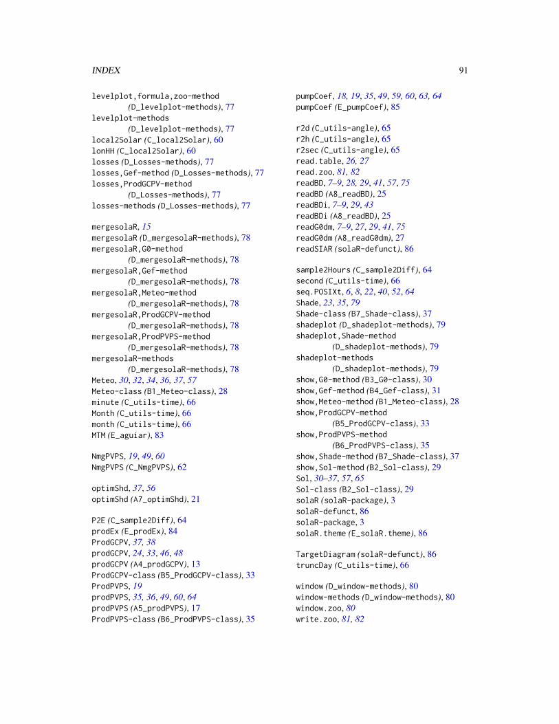
INDEX 91

levelplot,formula,zoo-method(D_levelplot-methods), 77

levelplot-methods(D_levelplot-methods), 77

local2Solar (C_local2Solar), 60lonHH (C_local2Solar), 60losses (D_Losses-methods), 77losses,Gef-method (D_Losses-methods), 77losses,ProdGCPV-method

(D_Losses-methods), 77losses-methods (D_Losses-methods), 77

mergesolaR, 15mergesolaR (D_mergesolaR-methods), 78mergesolaR,G0-method

(D_mergesolaR-methods), 78mergesolaR,Gef-method

(D_mergesolaR-methods), 78mergesolaR,Meteo-method

(D_mergesolaR-methods), 78mergesolaR,ProdGCPV-method

(D_mergesolaR-methods), 78mergesolaR,ProdPVPS-method

(D_mergesolaR-methods), 78mergesolaR-methods

(D_mergesolaR-methods), 78Meteo, 30, 32, 34, 36, 37, 57Meteo-class (B1_Meteo-class), 28minute (C_utils-time), 66Month (C_utils-time), 66month (C_utils-time), 66MTM (E_aguiar), 83

NmgPVPS, 19, 49, 60NmgPVPS (C_NmgPVPS), 62

optimShd, 37, 56optimShd (A7_optimShd), 21

P2E (C_sample2Diff), 64prodEx (E_prodEx), 84ProdGCPV, 37, 38prodGCPV, 24, 33, 46, 48prodGCPV (A4_prodGCPV), 13ProdGCPV-class (B5_ProdGCPV-class), 33ProdPVPS, 19prodPVPS, 35, 36, 49, 60, 64prodPVPS (A5_prodPVPS), 17ProdPVPS-class (B6_ProdPVPS-class), 35

pumpCoef, 18, 19, 35, 49, 59, 60, 63, 64pumpCoef (E_pumpCoef), 85

r2d (C_utils-angle), 65r2h (C_utils-angle), 65r2sec (C_utils-angle), 65read.table, 26, 27read.zoo, 81, 82readBD, 7–9, 28, 29, 41, 57, 75readBD (A8_readBD), 25readBDi, 7–9, 29, 43readBDi (A8_readBD), 25readG0dm, 7–9, 27, 29, 41, 75readG0dm (A8_readG0dm), 27readSIAR (solaR-defunct), 86

sample2Hours (C_sample2Diff), 64second (C_utils-time), 66seq.POSIXt, 6, 8, 22, 40, 52, 64Shade, 23, 35, 79Shade-class (B7_Shade-class), 37shadeplot (D_shadeplot-methods), 79shadeplot,Shade-method

(D_shadeplot-methods), 79shadeplot-methods

(D_shadeplot-methods), 79show,G0-method (B3_G0-class), 30show,Gef-method (B4_Gef-class), 31show,Meteo-method (B1_Meteo-class), 28show,ProdGCPV-method

(B5_ProdGCPV-class), 33show,ProdPVPS-method

(B6_ProdPVPS-class), 35show,Shade-method (B7_Shade-class), 37show,Sol-method (B2_Sol-class), 29Sol, 30–37, 57, 65Sol-class (B2_Sol-class), 29solaR (solaR-package), 3solaR-defunct, 86solaR-package, 3solaR.theme (E_solaR.theme), 86

TargetDiagram (solaR-defunct), 86truncDay (C_utils-time), 66

window (D_window-methods), 80window-methods (D_window-methods), 80window.zoo, 80write.zoo, 81, 82

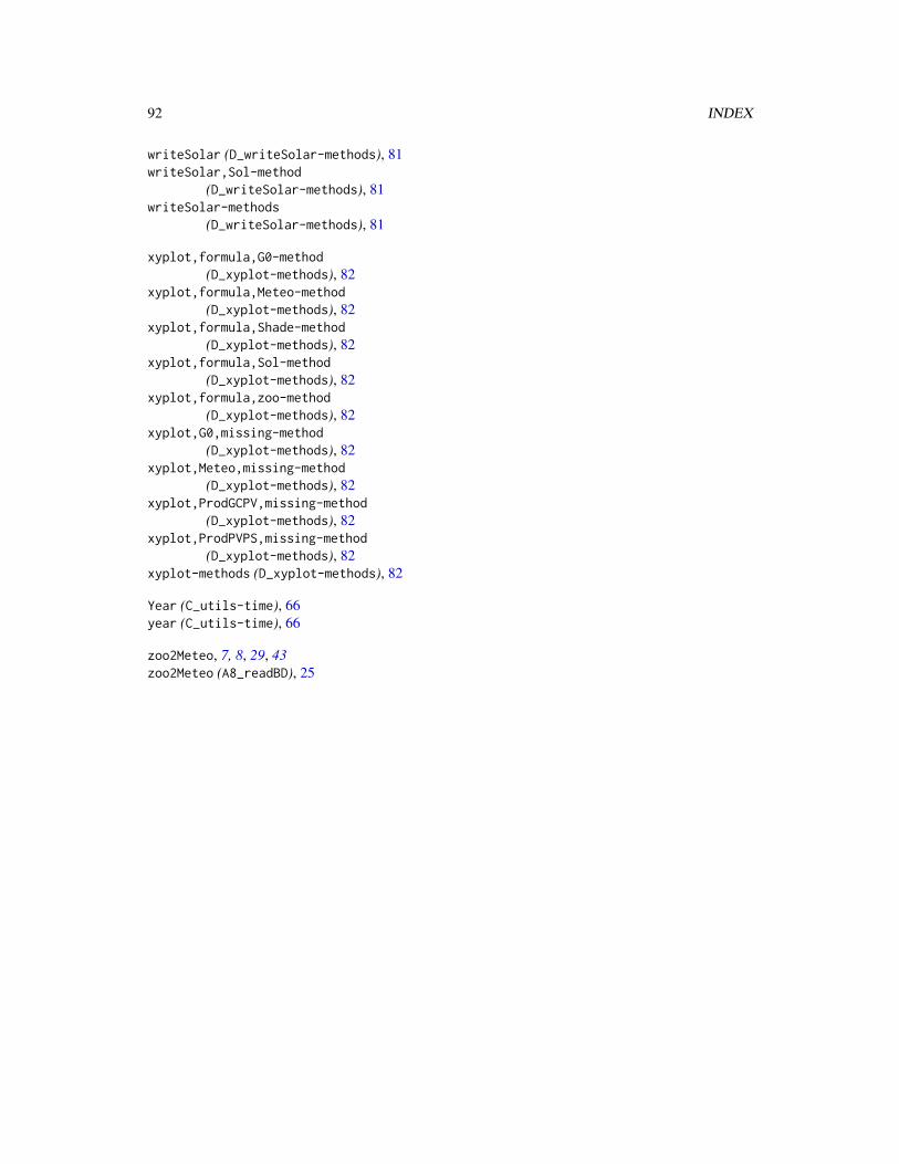
92 INDEX

writeSolar (D_writeSolar-methods), 81writeSolar,Sol-method

(D_writeSolar-methods), 81writeSolar-methods

(D_writeSolar-methods), 81

xyplot,formula,G0-method(D_xyplot-methods), 82

xyplot,formula,Meteo-method(D_xyplot-methods), 82

xyplot,formula,Shade-method(D_xyplot-methods), 82

xyplot,formula,Sol-method(D_xyplot-methods), 82

xyplot,formula,zoo-method(D_xyplot-methods), 82

xyplot,G0,missing-method(D_xyplot-methods), 82

xyplot,Meteo,missing-method(D_xyplot-methods), 82

xyplot,ProdGCPV,missing-method(D_xyplot-methods), 82

xyplot,ProdPVPS,missing-method(D_xyplot-methods), 82

xyplot-methods (D_xyplot-methods), 82

Year (C_utils-time), 66year (C_utils-time), 66

zoo2Meteo, 7, 8, 29, 43zoo2Meteo (A8_readBD), 25

package ‘solar’ - the comprehensive r archive network ‘solar’ august 29, 2016 type package...

Documents