package ‘msm’ - the comprehensive r archive network · package ‘msm’ february 2, 2018...

Package ‘msm’February 2, 2018

Version 1.6.6

Date 2018-02-02

Title Multi-State Markov and Hidden Markov Models in Continuous Time

Author Christopher Jackson <[email protected]>

Maintainer Christopher Jackson <[email protected]>

Description Functions for fitting continuous-time Markov and hiddenMarkov multi-state models to longitudinal data. Designed forprocesses observed at arbitrary times in continuous time (panel data)but some other observation schemes are supported. Both Markovtransition rates and the hidden Markov output process can be modelledin terms of covariates, which may be constant or piecewise-constantin time.

License GPL (>= 2)

Imports survival,mvtnorm,expm

Suggests mstate,minqa,doParallel,foreach,numDeriv,testthat,flexsurv

URL https://github.com/chjackson/msm

BugReports https://github.com/chjackson/msm/issues

LazyData yes

NeedsCompilation yes

Repository CRAN

Date/Publication 2018-02-02 18:37:56 UTC

R topics documented:2phase . . . . . . . . . . . . . . . . . . . . . . . . . . . . . . . . . . . . . . . . . . . . 3aneur . . . . . . . . . . . . . . . . . . . . . . . . . . . . . . . . . . . . . . . . . . . . 5boot.msm . . . . . . . . . . . . . . . . . . . . . . . . . . . . . . . . . . . . . . . . . . 6bos . . . . . . . . . . . . . . . . . . . . . . . . . . . . . . . . . . . . . . . . . . . . . . 9cav . . . . . . . . . . . . . . . . . . . . . . . . . . . . . . . . . . . . . . . . . . . . . . 10cmodel.object . . . . . . . . . . . . . . . . . . . . . . . . . . . . . . . . . . . . . . . . 11

1

https://github.com/chjackson/msm

https://github.com/chjackson/msm/issues

2 R topics documented:

coef.msm . . . . . . . . . . . . . . . . . . . . . . . . . . . . . . . . . . . . . . . . . . 11crudeinits.msm . . . . . . . . . . . . . . . . . . . . . . . . . . . . . . . . . . . . . . . 12deltamethod . . . . . . . . . . . . . . . . . . . . . . . . . . . . . . . . . . . . . . . . . 13draic.msm . . . . . . . . . . . . . . . . . . . . . . . . . . . . . . . . . . . . . . . . . . 15ecmodel.object . . . . . . . . . . . . . . . . . . . . . . . . . . . . . . . . . . . . . . . 18efpt.msm . . . . . . . . . . . . . . . . . . . . . . . . . . . . . . . . . . . . . . . . . . 18ematrix.msm . . . . . . . . . . . . . . . . . . . . . . . . . . . . . . . . . . . . . . . . 21emodel.object . . . . . . . . . . . . . . . . . . . . . . . . . . . . . . . . . . . . . . . . 22fev . . . . . . . . . . . . . . . . . . . . . . . . . . . . . . . . . . . . . . . . . . . . . . 23hazard.msm . . . . . . . . . . . . . . . . . . . . . . . . . . . . . . . . . . . . . . . . . 24hmm-dists . . . . . . . . . . . . . . . . . . . . . . . . . . . . . . . . . . . . . . . . . . 25hmmMV . . . . . . . . . . . . . . . . . . . . . . . . . . . . . . . . . . . . . . . . . . . 28hmodel.object . . . . . . . . . . . . . . . . . . . . . . . . . . . . . . . . . . . . . . . . 30logLik.msm . . . . . . . . . . . . . . . . . . . . . . . . . . . . . . . . . . . . . . . . . 32lrtest.msm . . . . . . . . . . . . . . . . . . . . . . . . . . . . . . . . . . . . . . . . . . 32MatrixExp . . . . . . . . . . . . . . . . . . . . . . . . . . . . . . . . . . . . . . . . . . 33medists . . . . . . . . . . . . . . . . . . . . . . . . . . . . . . . . . . . . . . . . . . . 35model.frame.msm . . . . . . . . . . . . . . . . . . . . . . . . . . . . . . . . . . . . . . 37msm . . . . . . . . . . . . . . . . . . . . . . . . . . . . . . . . . . . . . . . . . . . . . 38msm.form.qoutput . . . . . . . . . . . . . . . . . . . . . . . . . . . . . . . . . . . . . . 52msm.object . . . . . . . . . . . . . . . . . . . . . . . . . . . . . . . . . . . . . . . . . 53msm.summary . . . . . . . . . . . . . . . . . . . . . . . . . . . . . . . . . . . . . . . . 55msm2Surv . . . . . . . . . . . . . . . . . . . . . . . . . . . . . . . . . . . . . . . . . . 56odds.msm . . . . . . . . . . . . . . . . . . . . . . . . . . . . . . . . . . . . . . . . . . 58paramdata.object . . . . . . . . . . . . . . . . . . . . . . . . . . . . . . . . . . . . . . 59pearson.msm . . . . . . . . . . . . . . . . . . . . . . . . . . . . . . . . . . . . . . . . 61pexp . . . . . . . . . . . . . . . . . . . . . . . . . . . . . . . . . . . . . . . . . . . . . 65phasemeans.msm . . . . . . . . . . . . . . . . . . . . . . . . . . . . . . . . . . . . . . 66plot.msm . . . . . . . . . . . . . . . . . . . . . . . . . . . . . . . . . . . . . . . . . . 67plot.prevalence.msm . . . . . . . . . . . . . . . . . . . . . . . . . . . . . . . . . . . . 68plot.survfit.msm . . . . . . . . . . . . . . . . . . . . . . . . . . . . . . . . . . . . . . . 70plotprog.msm . . . . . . . . . . . . . . . . . . . . . . . . . . . . . . . . . . . . . . . . 72pmatrix.msm . . . . . . . . . . . . . . . . . . . . . . . . . . . . . . . . . . . . . . . . 73pmatrix.piecewise.msm . . . . . . . . . . . . . . . . . . . . . . . . . . . . . . . . . . . 75pnext.msm . . . . . . . . . . . . . . . . . . . . . . . . . . . . . . . . . . . . . . . . . . 77ppass.msm . . . . . . . . . . . . . . . . . . . . . . . . . . . . . . . . . . . . . . . . . . 79prevalence.msm . . . . . . . . . . . . . . . . . . . . . . . . . . . . . . . . . . . . . . . 81print.msm . . . . . . . . . . . . . . . . . . . . . . . . . . . . . . . . . . . . . . . . . . 84printold.msm . . . . . . . . . . . . . . . . . . . . . . . . . . . . . . . . . . . . . . . . 85psor . . . . . . . . . . . . . . . . . . . . . . . . . . . . . . . . . . . . . . . . . . . . . 86qcmodel.object . . . . . . . . . . . . . . . . . . . . . . . . . . . . . . . . . . . . . . . 87qgeneric . . . . . . . . . . . . . . . . . . . . . . . . . . . . . . . . . . . . . . . . . . . 88qmatrix.msm . . . . . . . . . . . . . . . . . . . . . . . . . . . . . . . . . . . . . . . . 89qmodel.object . . . . . . . . . . . . . . . . . . . . . . . . . . . . . . . . . . . . . . . . 91qratio.msm . . . . . . . . . . . . . . . . . . . . . . . . . . . . . . . . . . . . . . . . . 92recreate.olddata . . . . . . . . . . . . . . . . . . . . . . . . . . . . . . . . . . . . . . . 93scoreresid.msm . . . . . . . . . . . . . . . . . . . . . . . . . . . . . . . . . . . . . . . 94sim.msm . . . . . . . . . . . . . . . . . . . . . . . . . . . . . . . . . . . . . . . . . . . 95

2phase 3

simfitted.msm . . . . . . . . . . . . . . . . . . . . . . . . . . . . . . . . . . . . . . . . 96simmulti.msm . . . . . . . . . . . . . . . . . . . . . . . . . . . . . . . . . . . . . . . . 97sojourn.msm . . . . . . . . . . . . . . . . . . . . . . . . . . . . . . . . . . . . . . . . . 99statetable.msm . . . . . . . . . . . . . . . . . . . . . . . . . . . . . . . . . . . . . . . 101surface.msm . . . . . . . . . . . . . . . . . . . . . . . . . . . . . . . . . . . . . . . . . 102tnorm . . . . . . . . . . . . . . . . . . . . . . . . . . . . . . . . . . . . . . . . . . . . 103totlos.msm . . . . . . . . . . . . . . . . . . . . . . . . . . . . . . . . . . . . . . . . . . 105transient.msm . . . . . . . . . . . . . . . . . . . . . . . . . . . . . . . . . . . . . . . . 108updatepars.msm . . . . . . . . . . . . . . . . . . . . . . . . . . . . . . . . . . . . . . . 109viterbi.msm . . . . . . . . . . . . . . . . . . . . . . . . . . . . . . . . . . . . . . . . . 109

Index 111

2phase Coxian phase-type distribution with two phases

Description

Density, distribution, quantile functions and other utilities for the Coxian phase-type distributionwith two phases.

Usage

d2phase(x, l1, mu1, mu2, log=FALSE)p2phase(q, l1, mu1, mu2, lower.tail=TRUE, log.p=FALSE)q2phase(p, l1, mu1, mu2, lower.tail=TRUE, log.p=FALSE)r2phase(n, l1, mu1, mu2)h2phase(x, l1, mu1, mu2, log=FALSE)

Arguments

x,q vector of quantiles.

p vector of probabilities.

n number of observations. If length(n) > 1, the length is taken to be the numberrequired.

l1 Intensity for transition between phase 1 and phase 2.

mu1 Intensity for transition from phase 1 to exit.

mu2 Intensity for transition from phase 2 to exit.

log logical; if TRUE, return log density or log hazard.

log.p logical; if TRUE, probabilities p are given as log(p).

lower.tail logical; if TRUE (default), probabilities are P[X <= x], otherwise, P[X > x].

4 2phase

Details

This is the distribution of the time to reach state 3 in a continuous-time Markov model with threestates and transitions permitted from state 1 to state 2 (with intensity λ1) state 1 to state 3 (intensityµ1) and state 2 to state 3 (intensity µ2). States 1 and 2 are the two "phases" and state 3 is the "exit"state.

The density is

f(t|λ1, µ1) = e−(λ1+µ1)t(µ1 + (λ1 + µ1)λ1t)

if λ1 + µ1 = µ2, and

f(t|λ1, µ1, µ2) =(λ1 + µ1)e−(λ1+µ1)t(µ2 − µ1) + µ2λ1e

−µ2t

λ1 + µ1 − µ2

otherwise. The distribution function is

F (t|λ1, µ1) = 1− e−(λ1+µ1)t(1 + λ1t)

if λ1 + µ1 = µ2, and

F (t|λ1, µ1, µ2) = 1− e−(λ1+µ1)t(µ2 − µ1) + λ1e−µ2t

λ1 + µ1 − µ2

otherwise. Quantiles are calculated by numerically inverting the distribution function.

The mean is (1 + λ1/µ2)/(λ1 + µ1).

The variance is (2 + 2λ1(λ1 + µ1 + µ2)/µ22 − (1 + λ1/µ2)2)/(λ1 + µ1)2.

If µ1 = µ2 it reduces to an exponential distribution with rate µ1, and the parameter λ1 is redundant.Or also if λ1 = 0.

The hazard at x = 0 is µ1, and smoothly increasing if µ1 < µ2. If λ1 + µ1 ≥ µ2 it increases toan asymptote of µ2, and if λ1 + µ1 ≤ µ2 it increases to an asymptote of λ1 + µ1. The hazard isdecreasing if µ1 > µ2, to an asymptote of µ2.

Value

d2phase gives the density, p2phase gives the distribution function, q2phase gives the quantilefunction, r2phase generates random deviates, and h2phase gives the hazard.

Alternative parameterisation

An individual following this distribution can be seen as coming from a mixture of two populations:

1) "short stayers" whose mean sojourn time is M1 = 1/(λ1 + µ1) and sojourn distribution isexponential with rate λ1 + µ1.

2) "long stayers" whose mean sojourn time M2 = 1/(λ1 + µ1) + 1/µ2 and sojourn distribution isthe sum of two exponentials with rate λ1 +µ1 and µ2 respectively. The individual is a "long stayer"with probability p = λ1/(λ1 + µ1).

aneur 5

Thus a two-phase distribution can be more intuitively parameterised by the short and long staymeans M1 < M2 and the long stay probability p. Given these parameters, the transition intensitiesare λ1 = p/M1, µ1 = (1 − p)/M1, and µ2 = 1/(M2 −M1). This can be useful for choosingintuitively reasonable initial values for procedures to fit these models to data.

The hazard is increasing at least if M2 < 2M1, and also only if (M2 − 2M1)/(M2 −M1) < p.

For increasing hazards with λ1 + µ1 ≤ µ2, the maximum hazard ratio between any time t and time0 is 1/(1− p).

For increasing hazards with λ1 +µ1 ≥ µ2, the maximum hazard ratio is M1/((1− p)(M2−M1)).This is the minimum hazard ratio for decreasing hazards.

General phase-type distributions

This is a special case of the n-phase Coxian phase-type distribution, which in turn is a specialcase of the (general) phase-type distribution. The actuar R package implements a general n-phasedistribution defined by the time to absorption of a general continuous-time Markov chain with asingle absorbing state, where the process starts in one of the transient states with a given probability.

Author(s)

C. H. Jackson <[email protected]>

References

C. Dutang, V. Goulet and M. Pigeon (2008). actuar: An R Package for Actuarial Science. Journalof Statistical Software, vol. 25, no. 7, 1-37. URL http://www.jstatsoft.org/v25/i07

aneur Aortic aneurysm progression data

Description

This dataset contains longitudinal measurements of grades of aortic aneurysms, measured by ultra-sound examination of the diameter of the aorta.

Usage

aneur

Format

A data frame containing 4337 rows, with each row corresponding to an ultrasound scan from oneof 838 men over 65 years of age.

ptnum (numeric) Patient identification numberage (numeric) Recipient age at examination (years)

diam (numeric) Aortic diameterstate (numeric) State of aneurysm.

6 boot.msm

The states represent successive degrees of aneurysm severity, as indicated by the aortic diameter.

State 1 Aneurysm-free < 30 cmState 2 Mild aneurysm 30-44 cmState 3 Moderate aneurysm 45-54 cmState 4 Severe aneurysm > 55 cm

683 of these men were aneurysm-free at age 65 and were re-screened every two years. The remain-ing men were aneurysmal at entry and had successive screens with frequency depending on the stateof the aneurysm. Severe aneurysms are repaired by surgery.

Source

The Chichester, U.K. randomised controlled trial of screening for abdominal aortic aneurysms byultrasonography.

References

Jackson, C.H., Sharples, L.D., Thompson, S.G. and Duffy, S.W. and Couto, E. Multi-state Markovmodels for disease progression with classification error. The Statistician, 52(2): 193–209 (2003)

Couto, E. and Duffy, S. W. and Ashton, H. A. and Walker, N. M. and Myles, J. P. and Scott, R.A. P. and Thompson, S. G. (2002) Probabilities of progression of aortic aneurysms: estimates andimplications for screening policy Journal of Medical Screening 9(1):40–42

boot.msm Bootstrap resampling for multi-state models

Description

Draw a number of bootstrap resamples, refit a msm model to the resamples, and calculate statisticson the refitted models.

Usage

boot.msm(x, stat=pmatrix.msm, B=1000, file=NULL, cores=NULL)

Arguments

x A fitted msm model, as output by msm.

stat A function to call on each refitted msm model. By default this is pmatrix.msm,returning the transition probability matrix in one time unit. If NULL then nofunction is computed.

B Number of bootstrap resamples.

boot.msm 7

file Name of a file in which to save partial results after each replicate. This issaved using save and can be restored using load, producing an object calledboot.list containing the partial results. Not supported when using parallelprocessing.

cores Number of processor cores to use for parallel processing. Requires the doPar-allel package to be installed. If not specified, parallel processing is not used. Ifcores is set to the string "default", the default methods of makeCluster (onWindows) or registerDoParallel (on Unix-like) are used.

Details

The bootstrap datasets are computed by resampling independent transitions between pairs of states(for non-hidden models without censoring), or independent individual series (for hidden models ormodels with censoring). Therefore this approach doesn’t work if, for example, the data for a HMMconsist of a series of observations from just one individual, and is inaccurate for small numbers ofindependent transitions or individuals.

Confidence intervals or standard errors for the corresponding statistic can be calculated by sum-marising the returned list of B replicated outputs. This is currently implemented for most the out-put functions qmatrix.msm, ematrix.msm, qratio.msm, pmatrix.msm, pmatrix.piecewise.msm,totlos.msm and prevalence.msm. For other outputs, users will have to write their own code tosummarise the output of boot.msm.

Most of msm’s output functions present confidence intervals based on asymptotic standard errorscalculated from the Hessian. These are expected to be underestimates of the true standard errors(Cramer-Rao lower bound). Some of these functions use a further approximation, the delta method(see deltamethod) to obtain standard errors of transformed parameters. Bootstrapping should givea more accurate estimate of the uncertainty.

An alternative method which is less accurate though faster than bootstrapping, but more accuratethan the delta method, is to draw a sample from the asymptotic multivariate normal distribution im-plied by the maximum likelihood estimates (and covariance matrix), and summarise the transformedestimates. See pmatrix.msm.

All objects used in the original call to msm which produced x, such as the qmatrix, should be inthe working environment, or else boot.msm will produce an “object not found” error. This enablesboot.msm to refit the original model to the replicate datasets. However there is currently a limitation.In the original call to msm, the "formula" argument should be specified directly, as, for example,

msm(state ~ time, data = ...)

and not, for example,

form = data$state ~ data$time

msm(formula=form, data = ...)

otherwise boot.msm will be unable to draw the replicate datasets.

boot.msm will also fail with an incomprehensible error if the original call to msm used a used-defined object whose name is the same as a built-in R object, or an object in any other loadedpackage. For example, if you have called a Q matrix q, when q() is the built-in function forquitting R.

If stat is NULL, then B different msm model objects will be stored in memory. This is unadvisable,as msm objects tend to be large, since they contain the original data used for the msm fit, so this willbe wasteful of memory.

8 boot.msm

To specify more than one statistic, write a function consisting of a list of different function calls, forexample,

stat = function(x) list (pmatrix.msm(x, t=1), pmatrix.msm(x, t=2))

Value

A list with B components, containing the result of calling function stat on each of the refittedmodels. If stat is NULL, then each component just contains the refitted model. If one of the Bmodel fits was unsuccessful and resulted in an error, then the corresponding list component willcontain the error message.

Author(s)

C.H.Jackson <[email protected]>

References

Efron, B. and Tibshirani, R.J. (1993) An Introduction to the Bootstrap, Chapman and Hall.

See Also

qmatrix.msm, qratio.msm, sojourn.msm, ematrix.msm, pmatrix.msm, pmatrix.piecewise.msm,totlos.msm, prevalence.msm.

Examples

## Not run:## Psoriatic arthritis exampledata(psor)psor.q <- rbind(c(0,0.1,0,0),c(0,0,0.1,0),c(0,0,0,0.1),c(0,0,0,0))psor.msm <- msm(state ~ months, subject=ptnum, data=psor, qmatrix =psor.q, covariates = ~ollwsdrt+hieffusn,constraint = list(hieffusn=c(1,1,1),ollwsdrt=c(1,1,2)),control = list(REPORT=1,trace=2), method="BFGS")

## Bootstrap the baseline transition intensity matrix. This will take a long time.q.list <- boot.msm(psor.msm, function(x)x$Qmatrices$baseline)## Manipulate the resulting list of matrices to calculate bootstrap standard errors.apply(array(unlist(q.list), dim=c(4,4,5)), c(1,2), sd)## Similarly calculate a bootstrap 95% confidence intervalapply(array(unlist(q.list), dim=c(4,4,5)), c(1,2),

function(x)quantile(x, c(0.025, 0.975)))## Bootstrap standard errors are larger than the asymptotic standard## errors calculated from the Hessianpsor.msm$QmatricesSE$baseline

## End(Not run)

bos 9

bos Bronchiolitis obliterans syndrome after lung transplants

Description

A dataset containing histories of bronchiolitis obliterans syndrome (BOS) from lung transplantrecipients. BOS is a chronic decline in lung function, often observed after lung transplantation. Thecondition is classified into four stages of severity: none, mild, moderate and severe.

Usage

bos

Format

A data frame containing 638 rows, grouped by patient, including histories of 204 patients. Thefirst observation for each patient is defined to be stage 1, no BOS, at six months after transplant.Subsequent observations denote the entry times into stages 2, 3, 4, representing mild, moderate andsevere BOS respectively, and stage 5, representing death.

ptnum (numeric) Patient identification numbertime (numeric) Months after transplantstate (numeric) BOS state entered at this time

Details

The entry time of each patient into each stage of BOS was estimated by clinicians, based on theirhistory of lung function measurements and acute rejection and infection episodes. BOS is onlyassumed to occur beyond six months after transplant. In the first six months the function of eachpatient’s new lung stabilises. Subsequently BOS is diagnosed by comparing the lung functionagainst the "baseline" value.

The objects bos3 and bos4 contain the same data, but with mild/moderate/severe combined, andmoderate/severe combined, to give 3 and 4-state representations respectively.

Source

Papworth Hospital, U.K.

References

Heng. D. et al. (1998). Bronchiolitis Obliterans Syndrome: Incidence, Natural History, Prognosis,and Risk Factors. Journal of Heart and Lung Transplantation 17(12)1255–1263.

10 cav

cav Heart transplant monitoring data

Description

A series of approximately yearly angiographic examinations of heart transplant recipients. The stateat each time is a grade of cardiac allograft vasculopathy (CAV), a deterioration of the arterial walls.

Usage

cav

Format

A data frame containing 2846 rows. There are 622 patients, the rows are grouped by patient numberand ordered by years after transplant, with each row representing an examination and containingadditional covariates.

PTNUM (numeric) Patient identification numberage (numeric) Recipient age at examination (years)

years (numeric) Examination time (years after transplant)dage (numeric) Age of heart donor (years)sex (numeric) sex (0=male, 1=female)

pdiag (factor) Primary diagnosis (reason for transplant)IHD=ischaemic heart disease, IDC=idiopathic dilated cardiomyopathy.

cumrej (numeric) Cumulative number of acute rejection episodesstate (numeric) State at the examination.

State 1 represents no CAV, state 2 is mild/moderate CAVand state 3 is severe CAV. State 4 indicates death.

firstobs (numeric) 0 = record represents an angiogram or date of death.1 = record represents transplant (patient’s first observation)

statemax (numeric) Maximum observed state so far for this patient (added in version 1.5.1)

Source


References

Sharples, L.D. and Jackson, C.H. and Parameshwar, J. and Wallwork, J. and Large, S.R. (2003). Di-agnostic accuracy of coronary angiopathy and risk factors for post-heart-transplant cardiac allograftvasculopathy. Transplantation 76(4):679-82

cmodel.object 11

cmodel.object Developer documentation: censoring model object

Description

A list giving information about censored states, their labels in the data and what true states theyrepresent.

Value

ncens The number of distinct values used for censored observations in the state datasupplied to msm.

censor A vector of length ncens, giving the labels used for censored states in the data.

states A vector obtained by unlist()ing a list with ncens elements, each giving theset of true states that an observation with this label could be.

index Index into states for the first state corresponding to each censor, plus an extralength(states)+1.

See Also

msm.object.

coef.msm Extract model coefficients

Description

Extract the estimated log transition intensities and the corresponding linear effects of each covariate.

Usage

## S3 method for class 'msm'coef(object, ...)

Arguments

object A fitted multi-state model object, as returned by msm.

... (unused) further arguments passed to or from other methods.

12 crudeinits.msm

Value

If there is no misclassification, coef.msm returns a list of matrices. The first component, labelledlogbaseline, is a matrix containing the estimated transition intensities on the log scale with anycovariates fixed at their means in the data. Each remaining component is a matrix giving the lineareffects of the labelled covariate on the matrix of log intensities.

For misclassification models, coef.msm returns a list of lists. The first component, Qmatrices, is alist of matrices as described in the previous paragraph. The additional component Ematrices is alist of similar format containing the logit-misclassification probabilities and any estimated covariateeffects.

Author(s)


See Also

msm

crudeinits.msm Calculate crude initial values for transition intensities

Description

Calculates crude initial values for transition intensities by assuming that the data represent the exacttransition times of the Markov process.

Usage

crudeinits.msm(formula, subject, qmatrix, data=NULL, censor=NULL, censor.states=NULL)

Arguments

formula A formula giving the vectors containing the observed states and the correspond-ing observation times. For example,state ~ time

Observed states should be in the set 1, ..., n, where n is the number of states.Note hidden Markov models are not supported by this function.

subject Vector of subject identification numbers for the data specified by formula. Ifmissing, then all observations are assumed to be on the same subject. Thesemust be sorted so that all observations on the same subject are adjacent.

qmatrix Matrix of indicators for the allowed transitions. An initial value will be esti-mated for each value of qmatrix that is greater than zero. Transitions are takenas disallowed for each entry of qmatrix that is 0.

data An optional data frame in which the variables represented by subject andstate can be found.

deltamethod 13

censor A state, or vector of states, which indicates censoring. See msm.

censor.states Specifies the underlying states which censored observations can represent. Seemsm.

Details

Suppose we want a crude estimate of the transition intensity qrs from state r to state s. If we observenrs transitions from state r to state s, and a total of nr transitions from state r, then qrs/qrr can beestimated by nrs/nr. Then, given a total of Tr years spent in state r, the mean sojourn time 1/qrrcan be estimated as Tr/nr. Thus, nrs/Tr is a crude estimate of qrs.

If the data do represent the exact transition times of the Markov process, then these are the exactmaximum likelihood estimates.

Observed transitions which are incompatible with the given qmatrix are ignored. Censored statesare ignored.

Value

The estimated transition intensity matrix. This can be used as the qmatrix argument to msm.

Author(s)


See Also

statetable.msm

Examples

data(cav)twoway4.q <- rbind(c(-0.5, 0.25, 0, 0.25), c(0.166, -0.498, 0.166, 0.166),c(0, 0.25, -0.5, 0.25), c(0, 0, 0, 0))statetable.msm(state, PTNUM, data=cav)crudeinits.msm(state ~ years, PTNUM, data=cav, qmatrix=twoway4.q)

deltamethod The delta method

Description

Delta method for approximating the standard error of a transformation g(X) of a random variableX = (x1, x2, . . .), given estimates of the mean and covariance matrix of X .

Usage

deltamethod(g, mean, cov, ses=TRUE)

14 deltamethod

Arguments

g A formula representing the transformation. The variables must be labelled x1, x2,...For example,~ 1 / (x1 + x2)

If the transformation returns a vector, then a list of formulae representing (g1, g2, . . .)can be provided, for examplelist( ~ x1 + x2, ~ x1 / (x1 + x2) )

mean The estimated mean of X

cov The estimated covariance matrix of X

ses If TRUE, then the standard errors of g1(X), g2(X), . . . are returned. Otherwisethe covariance matrix of g(X) is returned.

Details

The delta method expands a differentiable function of a random variable about its mean, usuallywith a first-order Taylor approximation, and then takes the variance. For example, an approximationto the covariance matrix of g(X) is given by

Cov(g(X)) = g′(µ)Cov(X)[g′(µ)]T

where µ is an estimate of the mean of X . This function uses symbolic differentiation via deriv.

A limitation of this function is that variables created by the user are not visible within the formulag. To work around this, it is necessary to build the formula as a string, using functions such assprintf, then to convert the string to a formula using as.formula. See the example below.

If you can spare the computational time, bootstrapping is a more accurate method of calculatingconfidence intervals or standard errors for transformations of parameters. See boot.msm. Simu-lation from the asymptotic distribution of the MLEs (see e.g. Mandel 2013) is also a convenientalternative.

Value

A vector containing the standard errors of g1(X), g2(X), . . . or a matrix containing the covarianceof g(X).

Author(s)


References

Oehlert, G. W. (1992) A note on the delta method. American Statistician 46(1).

Mandel, M. (2013) Simulation based confidence intervals for functions with complicated deriva-tives. The American Statistician 67(2):76-81.

draic.msm 15

Examples

## Simple linear regression, E(y) = alpha + beta xx <- 1:100y <- rnorm(100, 4*x, 5)toy.lm <- lm(y ~ x)estmean <- coef(toy.lm)estvar <- summary(toy.lm)$cov.unscaled * summary(toy.lm)$sigma^2

## Estimate of (1 / (alphahat + betahat))1 / (estmean[1] + estmean[2])## Approximate standard errordeltamethod (~ 1 / (x1 + x2), estmean, estvar)

## We have a variable z we would like to use within the formula.z <- 1## deltamethod (~ z / (x1 + x2), estmean, estvar) will not work.## Instead, build up the formula as a string, and convert to a formula.form <- sprintf("~ %f / (x1 + x2)", z)formdeltamethod(as.formula(form), estmean, estvar)

draic.msm Criteria for comparing two multi-state models with nested state spaces

Description

A modification of Akaike’s information criterion, and a leave-one-out likelihood cross-validationcriterion, for comparing the predictive ability of two Markov multi-state models with nested statespaces. This is evaluated based on the restricted or aggregated data which the models have incommon.

Note that standard AIC can be computed for one or more fitted msm models x,y,... using AIC(x,y,...),and this can be used to compare models fitted to the same data. draic.msm and drlcv.msm are de-signed for models fitted to data with differently-aggregated state spaces.

Usage

draic.msm(msm.full, msm.coarse, likelihood.only=FALSE,information=c("expected","observed"), tl=0.95)

drlcv.msm(msm.full, msm.coarse, tl=0.95, cores=NULL,verbose=TRUE,outfile=NULL)

Arguments

msm.full Model on the bigger state space.

16 draic.msm

msm.coarse Model on the smaller state space.The two models must both be non-hidden Markov models without censoredstates.The two models must be fitted to the same datasets, except that the state spaceof the coarse model must be an aggregated version of the state space of the fullmodel. That is, every state in the full dataset must correspond to a unique state inthe coarse dataset. For example, for the full state variable c(1,1,2,2,3,4), thecorresponding coarse states could be c(1,1,2,2,2,3), but not c(1,2,3,4,4,4).The structure of allowed transitions in the coarse model must also be a collapsedversion of the big model structure, but no check is currently made for this in thecode.To use these functions, all objects which were used in the calls to fit msm.fulland msm.coarse must be in the working environment, for example, datasets anddefinitions of transition matrices.

likelihood.only

Don’t calculate Hessians and trace term (DRAIC).

information Use observed or expected information in the DRAIC trace term. Expected is thedefault, and much faster, though is only available for models fitted to pure paneldata (all obstype=1 in the call to msm, thus not exact transition times or exactdeath times)

tl Width of symmetric tracking interval, by default 0.95 for a 95% interval.

cores Number of processor cores to use in drlcv for cross-validation by parallel pro-cessing. Requires the doParallel package to be installed. If not specified, par-allel processing is not used. If cores is set to the string "default", the defaultmethods of makeCluster (on Windows) or registerDoParallel (on Unix-like) are used.

verbose Print intermediate results of each iteration of cross-validation to the consolewhile running. May not work with parallel processing.

outfile Output file to print intermediate results of cross-validation. Useful to track ex-ecution speed when using parallel processing, where output to the console maynot work.

Details

The difference in restricted AIC (Liquet and Commenges, 2011), as computed by this function, isdefined as

DRAIC = l(γn|x′′)− l(θn|x′′) + trace(J(θn|x′′)J(θn|x)−1 − J(γn|x′′)J(γn|x′)−1)

where γ and θ are the maximum likelihood estimates of the smaller and bigger models, fitted to thesmaller and bigger data, respectively.

l(γn|x′′) represents the likelihood of the simpler model evaluated on the restricted data.

l(θn|x′′) represents the likelihood of the complex model evaluated on the restricted data. This is ahidden Markov model, with a misclassification matrix and initial state occupancy probabilities asdescribed by Thom et al (2014).

draic.msm 17

J() are the corresponding (expected or observed, as specified by the user) information matrices.

x is the expanded data, to which the bigger model was originally fitted, and x′ is the data to whichthe smaller model was originally fitted. x′′ is the restricted data which the two models have incommon. x′′ = x′ in this implementation, so the models are nested.

The difference in likelihood cross-validatory criteria (Liquet and Commenges, 2011) is defined as

DRLCV = 1/n

n∑i=1

log(hX′′(x′′i |γ−i)/gX′′(x′′i |θ−i))

where γ−i and θ−i are the maximum likelihood estimates from the smaller and bigger models fittedto datasets with subject i left out, g() and h() are the densities of the corresponding models, and x′′iis the restricted data from subject i.

Tracking intervals are analogous to confidence intervals, but not strictly the same, since the quan-tity which D_RAIC aims to estimate, the difference in expected Kullback-Leibler discrepancy forpredicting a replicate dataset, depends on the sample size. See the references.

Positive values for these criteria indicate the coarse model is preferred, while negative values indi-cate the full model is preferred.

Value

A list containing DRAIC (draic.msm) or DRLCV (drlcv.msm), its component terms, and trackingintervals.

Author(s)

C. H. Jackson <[email protected]>, H. H. Z. Thom <[email protected]>

References

Thom, H. and Jackson, C. and Commenges, D. and Sharples, L. (2015) State selection in multistatemodels with application to quality of life in psoriatic arthritis. Statistics In Medicine 34(16) 2381 -2480.

Liquet, B. and Commenges D. (2011) Choice of estimators based on different observations: Modi-fied AIC and LCV criteria. Scandinavian Journal of Statistics; 38:268-287.

See Also

logLik.msm

18 efpt.msm

ecmodel.object Developer documentation: model for covariates on misclassificationprobabilities

Description

A list representing the model for covariates on misclassification probabilities.

Value

npars Number of covariate effect parameters. This is defined as the number of covari-ates on misclassification (with factors expanded as contrasts) multiplied by thenumber of allowed misclassifications in the model.

ndpars Number of distinct covariate effect parameters, as npars, but after any equalityconstraints have been applied.

ncovs Number of covariates on misclassification, with factors expanded as contrasts.

constr List of equality constraints on these covariate effects, as supplied in the miscconstraintargument to msm.

covlabels Names / labels of these covariates in the model matrix (see model.matrix.msm).

inits Initial values for these covariate effects, as a vector formed from the misccovinitslist supplied to msm.

covmeans Means of these covariates in the data (excluding data not required to fit themodel, such as observations with missing data in other elements or subjects’ lastobservations). This includes means of 0/1 factor contrasts as well as continuouscovariates (for historic reasons, which may not be sensible).

See Also

msm.object.

efpt.msm Expected first passage time

Description

Expected time until first reaching a particular state or set of states in a Markov model.

Usage

efpt.msm(x=NULL, qmatrix=NULL, tostate, start="all", covariates="mean",ci=c("none","normal","bootstrap"), cl=0.95, B=1000,cores=NULL, ...)

efpt.msm 19

Arguments

x A fitted multi-state model, as returned by msm.

qmatrix Instead of x, you can simply supply a transition intensity matrix in qmatrix.

tostate State, or set of states supplied as a vector, for which to estimate the first passagetime into. Can be integer, or character matched to the row names of the Q matrix.

start Starting state (integer). By default (start="all"), this will return a vector ofexpected passage times from each state in turn.Alternatively, this can be used to obtain the expected first passage time from aset of states, rather than single states. To achieve this, state is set to a vector ofweights, with length equal to the number of states in the model. These weightsshould be proportional to the probability of starting in each of the states in thedesired set, so that weights of zero are supplied for other states. The functionwill calculate the weighted average of the expected passage times from each ofthe corresponding states.

covariates Covariate values defining the intensity matrix for the fitted model x, as suppliedto qmatrix.msm.

ci If "normal", then calculate a confidence interval by simulating B random vectorsfrom the asymptotic multivariate normal distribution implied by the maximumlikelihood estimates (and covariance matrix) of the log transition intensities andcovariate effects.If "bootstrap" then calculate a confidence interval by non-parametric bootstraprefitting. This is 1-2 orders of magnitude slower than the "normal" method, butis expected to be more accurate. See boot.msm for more details of bootstrappingin msm.If "none" (the default) then no confidence interval is calculated.

cl Width of the symmetric confidence interval, relative to 1.

B Number of bootstrap replicates.

cores Number of cores to use for bootstrapping using parallel processing. See boot.msmfor more details.

... Arguments to pass to MatrixExp.

Details

The expected first passage times from each of a set of states i to to the remaining set of states i inthe state space, for a model with transition intensity matrix Q, are

−Q−1i,i 1

where 1 is a vector of ones, and Qi,i is the square subset of Q pertaining to states i.

It is equal to the sum of mean sojourn times for all states between the "from" and "to" states in aunidirectional model. If there is non-zero chance of reaching an absorbing state before reachingtostate, then it is infinite. It is trivially zero if the "from" state equals tostate.

This function currently only handles time-homogeneous Markov models. For time-inhomogeneousmodels it will assume that Q equals the average intensity matrix over all times and observed covari-ates. Simulation might be used to handle time dependence.

20 efpt.msm

Note this is the expectation of first passage time, and the confidence intervals are CIs for this mean,not predictive intervals for the first passage time. The full distribution of the first passage time to aset of states can be obtained by setting the rows of the intensity matrix Q corresponding to that setof states to zero to make a model where those states are absorbing. The corresponding transitionprobability matrix Exp(Qt) then gives the probabilities of having hit or passed that state by a timet (see the example below). This is implemented in ppass.msm.

Value

A vector of expected first passage times, or "hitting times", from each state to the desired state.

Author(s)


References

Norris, J. R. (1997) Markov Chains. Cambridge University Press.

See Also

sojourn.msm, totlos.msm, boot.msm.

Examples

twoway4.q <- rbind(c(-0.5, 0.25, 0, 0.25), c(0.166, -0.498, 0.166, 0.166),c(0, 0.25, -0.5, 0.25), c(0, 0, 0, 0))

efpt.msm(qmatrix=twoway4.q, tostate=3)# given in state 1, expected time to reaching state 3 is infinite# since may die (state 4) before entering state 3

# If we remove the death state from the model, EFPTs become finiteQ <- twoway4.q[1:3,1:3]; diag(Q) <- 0; diag(Q) <- -rowSums(Q)efpt.msm(qmatrix=Q, tostate=3)

# Suppose we cannot die or regress while in state 2, can only go to state 3Q <- twoway4.q; Q[2,4] <- Q[2,1] <- 0; diag(Q) <- 0; diag(Q) <- -rowSums(Q)efpt.msm(qmatrix=Q, tostate=3)# The expected time from 2 to 3 now equals the mean sojourn time in 2.-1/Q[2,2]

# Calculate cumulative distribution of the first passage time# into state 3 for the following three-state modelQ <- twoway4.q[1:3,1:3]; diag(Q) <- 0; diag(Q) <- -rowSums(Q)# Firstly form a model where the desired hitting state is absorbingQ[3,] <- 0MatrixExp(Q, t=10)[,3]ppass.msm(qmatrix=Q, tot=10)# Given in state 1 at time 0, P(hit 3 by time 10) = 0.479MatrixExp(Q, t=50)[,3] # P(hit 3 by time 50) = 0.98ppass.msm(qmatrix=Q, tot=50)

ematrix.msm 21

ematrix.msm Misclassification probability matrix

Description

Extract the estimated misclassification probability matrix, and corresponding confidence intervals,from a fitted multi-state model at a given set of covariate values.

Usage

ematrix.msm(x, covariates="mean", ci=c("delta","normal","bootstrap","none"),cl=0.95, B=1000, cores=NULL)

Arguments


covariates The covariate values for which to estimate the misclassification probability ma-trix. This can either be:

the string "mean", denoting the means of the covariates in the data (this is thedefault),

the number 0, indicating that all the covariates should be set to zero,

or a list of values, with optional names. For examplelist (60, 1)

where the order of the list follows the order of the covariates originally given inthe model formula, or a named list,list (age = 60, sex = 1)

ci If "delta" (the default) then confidence intervals are calculated by the deltamethod, or by simple transformation of the Hessian in the very simplest cases.If "normal", then calculate a confidence interval by simulating B random vec-tors from the asymptotic multivariate normal distribution implied by the max-imum likelihood estimates (and covariance matrix) of the multinomial-logit-transformed misclassification probabilities and covariate effects, then transform-ing back.If "bootstrap" then calculate a confidence interval by non-parametric bootstraprefitting. This is 1-2 orders of magnitude slower than the "normal" method, butis expected to be more accurate. See boot.msm for more details of bootstrappingin msm.

cl Width of the symmetric confidence interval to present. Defaults to 0.95.

B Number of bootstrap replicates, or number of normal simulations from the dis-tribution of the MLEs


22 emodel.object

Details

Misclassification probabilities and covariate effects are estimated on the multinomial-logit scale bymsm. A covariance matrix is estimated from the Hessian of the maximised log-likelihood. Fromthese, the delta method can be used to obtain standard errors of the probabilities on the naturalscale at arbitrary covariate values. Confidence intervals are estimated by assuming normality on themultinomial-logit scale.

Value

A list with components:

estimate Estimated misclassification probability matrix. The rows correspond to truestates, and columns observed states.

SE Corresponding approximate standard errors.

L Lower confidence limits.

U Upper confidence limits.

Or if ci="none", then ematrix.msm just returns the estimated misclassification probability matrix.

The default print method for objects returned by ematrix.msm presents estimates and confidencelimits. To present estimates and standard errors, do something like

ematrix.msm(x)[c("estimates","SE")]

Author(s)


See Also

qmatrix.msm

emodel.object Developer documentation: misclassification model structure object

Description

A list giving information about the misclassifications assumed in a multi-state model fitted with theematrix argument of msm. Returned in a fitted msm model object. This information is convertedinternally to a hmodel object (see hmodel.object) for use in likelihood computations.

fev 23

Value

nstates Number of states (same as qmodel$nstates).

npars Number of allowed misclassifications, equal to sum(imatrix).

imatrix Indicator matrix for allowed misclassifications. This has (r, s) entry 1 if mis-classification of true state r as observed state s is possible. diagonal entries arearbitrarily set to 0.

ematrix Matrix of initial values for the misclassification probabilities, supplied as theematrix argument of msm.

inits Vector of these initial values, reading across rows of qmatrix and excluding thediagonal and disallowed transitions.

constr Indicators for equality constraints on baseline misclassification probabilities,taken from the econstraint argument to msm, and mapped if necessary to theset (1,2,3,...)

ndpars Number of distinct misclassification probabilities, after applying equality con-straints.

nipars Number of initial state occupancy probabilities being estimated. This is zero ifest.initprobs=FALSE, otherwise equal to the number of states.

initprobs Initial state occupancy probabilities, as supplied to msm (initial values beforeestimation, if est.initprobs=TRUE.)

est.initprobs Are initial state occupancy probabilities estimated (TRUE or FALSE), as suppliedin the est.initprobs argument of msm.

See Also

msm.object,qmodel.object, hmodel.object.

fev FEV1 measurements from lung transplant recipients

Description

A series of measurements of the forced expiratory volume in one second (FEV1) from lung trans-plant recipients, from six months onwards after their transplant.

Usage

fev

Format

A data frame containing 5896 rows. There are 204 patients, the rows are grouped by patient num-ber and ordered by days after transplant. Each row represents an examination and containing anadditional covariate.

24 hazard.msm

ptnum (numeric) Patient identification number.days (numeric) Examination time (days after transplant).fev (numeric) Percentage of baseline FEV1. A code of 999 indicates the patient’s date of death.

acute (numeric) 0/1 indicator for whether the patient suffered an acute infection or rejectionwithin 14 days of the visit.

Details

A baseline "normal" FEV1 for each individual is calculated using measurements from the first sixmonths after transplant. After six months, as presented in this dataset, FEV1 is expressed as apercentage of the baseline value.

FEV1 is monitored to diagnose bronchiolitis obliterans syndrome (BOS), a long-term lung functiondecline, thought to be a form of chronic rejection. Acute rejections and infections also affect thelung function in the short term.

Source


References

Jackson, C.H. and Sharples, L.D. Hidden Markov models for the onset and progression of bron-chiolitis obliterans syndrome in lung transplant recipients Statistics in Medicine, 21(1): 113–128(2002).

hazard.msm Calculate tables of hazard ratios for covariates on transition intensi-ties

Description

Hazard ratios are computed by exponentiating the estimated covariate effects on the log-transitionintensities. This function is called by summary.msm.

Usage

hazard.msm(x, hazard.scale = 1, cl = 0.95)

Arguments

x Output from msm representing a fitted multi-state model.

hazard.scale Vector with same elements as number of covariates on transition rates. Corre-sponds to the increase in each covariate used to calculate its hazard ratio. De-faults to all 1.


hmm-dists 25

Value

A list of tables containing hazard ratio estimates, one table for each covariate. Each table hasthree columns, containing the hazard ratio, and an approximate upper and lower confidence limitrespectively (assuming normality on the log scale), for each Markov chain transition intensity.

Author(s)


See Also

msm, summary.msm, odds.msm

hmm-dists Hidden Markov model constructors

Description

These functions are used to specify the distribution of the response conditionally on the underlyingstate in a hidden Markov model. A list of these function calls, with one component for each state,should be used for the hmodel argument to msm. The initial values for the parameters of the distri-bution should be given as arguments. Note the initial values should be supplied as literal values -supplying them as variables is currently not supported.

Usage

hmmCat(prob, basecat)hmmIdent(x)hmmUnif(lower, upper)hmmNorm(mean, sd)hmmLNorm(meanlog, sdlog)hmmExp(rate)hmmGamma(shape, rate)hmmWeibull(shape, scale)hmmPois(rate)hmmBinom(size, prob)hmmTNorm(mean, sd, lower, upper)hmmMETNorm(mean, sd, lower, upper, sderr, meanerr=0)hmmMEUnif(lower, upper, sderr, meanerr=0)hmmNBinom(disp, prob)hmmBeta(shape1,shape2)hmmT(mean,scale,df)

26 hmm-dists

Arguments

prob (hmmCat) Vector of probabilities of observing category 1, 2, ..., length(prob)respectively. Or the probability governing a binomial or negative binomial dis-tribution.

basecat (hmmCat) Category which is considered to be the "baseline", so that during esti-mation, the probabilities are parameterised as probabilities relative to this base-line category. By default, the category with the greatest probability is used asthe baseline.

x (hmmIdent) Code in the data which denotes the exactly-observed state.

mean (hmmNorm,hmmLNorm,hmmTNorm) Mean defining a Normal, or truncated Normaldistribution.

sd (hmmNorm,hmmLNorm,hmmTNorm) Standard deviation defining a Normal, or trun-cated Normal distribution.

meanlog (hmmNorm,hmmLNorm,hmmTNorm) Mean on the log scale, for a log Normal distri-bution.

sdlog (hmmNorm,hmmLNorm,hmmTNorm) Standard deviation on the log scale, for a logNormal distribution.

rate (hmmPois,hmmExp,hmmGamma) Rate of a Poisson, Exponential or Gamma distri-bution (see dpois, dexp, dgamma).

shape (hmmPois,hmmExp,hmmGamma) Shape parameter of a Gamma or Weibull distri-bution (see dgamma, dweibull).

shape1,shape2 First and second parameters of a beta distribution (see dbeta).

scale (hmmGamma) Scale parameter of a Gamma distribution (see dgamma), or unstan-dardised Student t distribution.

df Degrees of freedom of the Student t distribution.

size Order of a Binomial distribution (see dbinom).

disp Dispersion parameter of a negative binomial distribution, also called size ororder. (see dnbinom).

lower (hmmUnif,hmmTNorm,hmmMEUnif) Lower limit for an Uniform or truncated Nor-mal distribution.

upper (hmmUnif,hmmTNorm,hmmMEUnif) Upper limit for an Uniform or truncated Nor-mal distribution.

sderr (hmmMETNorm,hmmUnif) Standard deviation of the Normal measurement errordistribution.

meanerr (hmmMETNorm,hmmUnif) Additional shift in the measurement error, fixed to 0 bydefault. This may be modelled in terms of covariates.

Details

hmmCat represents a categorical response distribution on the set 1, 2, ..., length(prob). TheMarkov model with misclassification is an example of this type of model. The categories in thiscase are (some subset of) the underlying states.

The hmmIdent distribution is used for underlying states which are observed exactly without error.

hmm-dists 27

hmmUnif, hmmNorm, hmmLNorm, hmmExp, hmmGamma, hmmWeibull, hmmPois, hmmBinom, hmmTNorm,hmmNBinom and hmmBeta represent Uniform, Normal, log-Normal, exponential, Gamma, Weibull,Poisson, Binomial, truncated Normal, negative binomial and beta distributions, respectively, withparameterisations the same as the default parameterisations in the corresponding base R distributionfunctions.

hmmT is the Student t distribution with general mean µ, scale σ and degrees of freedom df. Thevariance is σ2df/(df + 2). Note the t distribution in base R dt is a standardised one with mean 0and scale 1. These allow any positive (integer or non-integer) df. By default, all three parameters,including df, are estimated when fitting a hidden Markov model, but in practice, df might need tobe fixed for identifiability - this can be done using the fixedpars argument to msm.

The hmmMETNorm and hmmMEUnif distributions are truncated Normal and Uniform distributions,but with additional Normal measurement error on the response. These are generalisations of thedistributions proposed by Satten and Longini (1996) for modelling the progression of CD4 cellcounts in monitoring HIV disease. See medists for density, distribution, quantile and randomgeneration functions for these distributions. See also tnorm for density, distribution, quantile andrandom generation functions for the truncated Normal distribution.

See the PDF manual ‘msm-manual.pdf’ in the ‘doc’ subdirectory for algebraic definitions of allthese distributions. New hidden Markov model response distributions can be added to msm byfollowing the instructions in Section 2.17.1.

Parameters which can be modelled in terms of covariates, on the scale of a link function, are asfollows.

PARAMETER NAME LINK FUNCTIONmean identitymeanlog identityrate logscale logmeanerr identityprob (multinomial logistic regression)

Parameters basecat, lower, upper, size, meanerr are fixed at their initial values. All otherparameters are estimated while fitting the hidden Markov model, unless the appropriate fixedparsargument is supplied to msm.

For categorical response distributions (hmmCat) the outcome probabilities initialized to zero arefixed at zero, and the probability corresponding to basecat is fixed to one minus the sum of theremaining probabilities. These remaining probabilities are estimated, and can be modelled in termsof covariates via multinomial logistic regression (relative to basecat).

Value

Each function returns an object of class hmodel, which is a list containing information about themodel. The only component which may be useful to end users is r, a function of one argument nwhich returns a random sample of size n from the given distribution.

Author(s)


28 hmmMV

References

Satten, G.A. and Longini, I.M. Markov chains with measurement error: estimating the ’true’ courseof a marker of the progression of human immunodeficiency virus disease (with discussion) AppliedStatistics 45(3): 275-309 (1996).

Jackson, C.H. and Sharples, L.D. Hidden Markov models for the onset and progresison of bron-chiolitis obliterans syndrome in lung transplant recipients Statistics in Medicine, 21(1): 113–128(2002).

Jackson, C.H., Sharples, L.D., Thompson, S.G. and Duffy, S.W. and Couto, E. Multi-state Markovmodels for disease progression with classification error. The Statistician, 52(2): 193–209 (2003).

See Also

msm

hmmMV Multivariate hidden Markov models

Description

Constructor for a a multivariate hidden Markov model (HMM) where each of the n variables ob-served at the same time has a (potentially different) standard univariate distribution conditionallyon the underlying state. The n outcomes are independent conditionally on the hidden state.

If a particular state in a HMM has such an outcome distribution, then a call to hmmMV is supplied asthe corresponding element of the hmodel argument to msm. See Example 2 below.

A multivariate HMM where multiple outcomes at the same time are generated from the same dis-tribution is specified in the same way as the corresponding univariate model, so that hmmMV is notrequired. The outcome data are simply supplied as a matrix instead of a vector. See Example 1below.

The outcome data for such models are supplied as a matrix, with number of columns equal to themaximum number of arguments supplied to the hmmMV calls for each state. If some but not all of thevariables are missing (NA) at a particular time, then the observed data at that time still contribute tothe likelihood. The missing data are assumed to be missing at random. The Viterbi algorithm maybe used to predict the missing values given the fitted model and the observed data.

Typically the outcome model for each state will be from the same family or set of families, but withdifferent parameters. Theoretically, different numbers of distributions may be supplied for differentstates. If a particular state has fewer outcomes than the maximum, then the data for that state aretaken from the first columns of the response data matrix. However this is not likely to be a usefulmodel, since the number of observations will probably give information about the underlying state,violating the missing at random assumption.

Models with outcomes that are dependent conditionally on the hidden state (e.g. correlated multi-variate normal observations) are not currently supported.

Usage

hmmMV(...)

hmmMV 29

Arguments

... The number of arguments supplied should equal the maximum number of obser-vations made at one time. Each argument represents the univariate distributionof that outcome conditionally on the hidden state, and should be the result ofcalling a univariate hidden Markov model constructor (see hmm-dists).

Value

A list of objects, each of class hmmdist as returned by the univariate HMM constructors documentedin hmm-dists. The whole list has class hmmMVdist, which inherits from hmmdist.

Author(s)


References

Jackson, C. H., Su, L., Gladman, D. D. and Farewell, V. T. (2015) On modelling minimal diseaseactivity. Arthritis Care and Research (early view).

See Also

hmm-dists,msm

Examples

## Simulate data from a Markov modelnsubj <- 30; nobspt <- 5sim.df <- data.frame(subject = rep(1:nsubj, each=nobspt),

time = seq(0, 20, length=nobspt))set.seed(1)two.q <- rbind(c(-0.1, 0.1), c(0, 0))dat <- simmulti.msm(sim.df[,1:2], qmatrix=two.q, drop.absorb=FALSE)

### EXAMPLE 1## Generate two observations at each time from the same outcome## distribution:## Bin(40, 0.1) for state 1, Bin(40, 0.5) for state 2dat$obs1[dat$state==1] <- rbinom(sum(dat$state==1), 40, 0.1)dat$obs2[dat$state==1] <- rbinom(sum(dat$state==1), 40, 0.1)dat$obs1[dat$state==2] <- rbinom(sum(dat$state==2), 40, 0.5)dat$obs2[dat$state==2] <- rbinom(sum(dat$state==2), 40, 0.5)dat$obs <- cbind(obs1 = dat$obs1, obs2 = dat$obs2)

## Fitted model should approximately recover true parametersmsm(obs ~ time, subject=subject, data=dat, qmatrix=two.q,

hmodel = list(hmmBinom(size=40, prob=0.2),hmmBinom(size=40, prob=0.2)))

### EXAMPLE 2## Generate two observations at each time from different

30 hmodel.object

## outcome distributions:## Bin(40, 0.1) and Bin(40, 0.2) for state 1,dat$obs1 <- dat$obs2 <- NAdat$obs1[dat$state==1] <- rbinom(sum(dat$state==1), 40, 0.1)dat$obs2[dat$state==1] <- rbinom(sum(dat$state==1), 40, 0.2)

## Bin(40, 0.5) and Bin(40, 0.6) for state 2dat$obs1[dat$state==2] <- rbinom(sum(dat$state==2), 40, 0.6)dat$obs2[dat$state==2] <- rbinom(sum(dat$state==2), 40, 0.5)dat$obs <- cbind(obs1 = dat$obs1, obs2 = dat$obs2)

## Fitted model should approximately recover true parametersmsm(obs ~ time, subject=subject, data=dat, qmatrix=two.q,

hmodel = list(hmmMV(hmmBinom(size=40, prob=0.3),hmmBinom(size=40, prob=0.3)),

hmmMV(hmmBinom(size=40, prob=0.3),hmmBinom(size=40, prob=0.3))),

control=list(maxit=10000))

hmodel.object Developer documentation: hidden Markov model structure object

Description

A list giving information about the models for the outcome data conditionally on the states of ahidden Markov model. Used in internal computations, and returned in a fitted msm model object.

Value

hidden TRUE for hidden Markov models, FALSE otherwise.

nstates Number of states, the same as qmodel$nstates.

fitted TRUE if the parameter values in pars are the maximum likelihood estimates,FALSE if they are the initial values.

models The outcome distribution for each hidden state. A vector of length nstateswhose rth entry is the index of the state r outcome distributions in the vector ofsupported distributions. The vector of supported distributions is given in full bymsm:::.msm.HMODELS: the first few are 1 for categorical outcome, 2 for identity,3 for uniform and 4 for normal.

labels String identifying each distribution in models.

npars Vector of length nstates giving the number of parameters in each outcomedistribution, excluding covariate effects.

nipars Number of initial state occupancy probabilities being estimated. This is zero ifest.initprobs=FALSE, otherwise equal to the number of states.

totpars Total number of parameters, equal to sum(npars).

pars A vector of length totpars, made from concatenating a list of length nstateswhose rth component is vector of the parameters for the state r outcome distri-bution.

hmodel.object 31

plabs List with the names of the parameters in pars.

parstate A vector of length totpars, whose ith element is the state corresponding to theith parameter.

firstpar A vector of length nstates giving the index in pars of the first parameter foreach state.

locpars Index in pars of parameters which can have covariates on them.

initprobs Initial state occupancy probabilities, as supplied to msm (initial values beforeestimation, if est.initprobs=TRUE.)

est.initprobs Are initial state occupancy probabilities estimated (TRUE or FALSE), as suppliedin the est.initprobs argument of msm.

ncovs Number of covariate effects per parameter in pars, with, e.g. factor contrastsexpanded.

coveffect Vector of covariate effects, of length sum(ncovs).

covlabels Labels of these effects.

coveffstate Vector indicating state corresponding to each element of coveffect.

ncoveffs Number of covariate effects on HMM outcomes, equal to sum(ncovs).

nicovs Vector of length nstates-1 giving the number of covariate effects on each initialstate occupancy probability (log relative to the baseline probability).

icoveffect Vector of length sum(nicovs) giving covariate effects on initial state occupancyprobabilities.

nicoveffs Number of covariate effects on initial state occupancy probabilities, equal tosum(nicovs).

constr Constraints on (baseline) hidden Markov model outcome parameters, as sup-plied in the hconstraint argument of msm, excluding covariate effects, con-verted to a vector and mapped to the set 1,2,3,. . . if necessary.

covconstr Vector of constraints on covariate effects in hidden Markov outcome models, assupplied in the hconstraint argument of msm, excluding baseline parameters,converted to a vector and mapped to the set 1,2,3,. . . if necessary.

ranges Matrix of range restrictions for HMM parameters, including those given to thehranges argument to msm.

foundse TRUE if standard errors are available for the estimates.

initpmat Matrix of initial state occupancy probabilities with one row for each subject(estimated if est.initprobs=TRUE).

ci Confidence intervals for baseline HMM outcome parameters.

covci Confidence intervals for covariate effects in HMM outcome models.

See Also

msm.object,qmodel.object, emodel.object.

32 lrtest.msm

logLik.msm Extract model log-likelihood

Description

Extract the log-likelihood and the number of parameters of a model fitted with msm.

Usage

## S3 method for class 'msm'logLik(object, by.subject=FALSE, ...)

Arguments


by.subject Return vector of subject-specific log-likelihoods, which should sum to the totallog-likelihood.

... (unused) further arguments passed to or from other methods.

Value

The log-likelihood of the model represented by ’object’ evaluated at the maximum likelihood esti-mates.

Akaike’s information criterion can also be computed using AIC(object).

Author(s)


See Also

msm,lrtest.msm.

lrtest.msm Likelihood ratio test

Description

Likelihood ratio test between two or more fitted multi-state models

Usage

lrtest.msm(...)

MatrixExp 33

Arguments

... Two or more fitted multi-state models, as returned by msm, ordered by increasingnumbers of parameters.

Value

A matrix with three columns, giving the likelihood ratio statistic, difference in degrees of freedomand the chi-squared p-value for a comparison of the first model supplied with each subsequentmodel.

Warning

The comparison between models will only be valid if they are fitted to the same dataset. This maybe a problem if there are missing values and R’s default of ’na.action = na.omit’ is used.

The likelihood ratio statistic only has the indicated chi-squared distribution if the models are nested.An alternative for comparing non-nested models is Akaike’s information criterion. This can becomputed for one or more fitted msm models x,y,... using AIC(x,y,...).

See Also

logLik.msm,msm

MatrixExp Matrix exponential

Description

Calculates the exponential of a square matrix.

Usage

MatrixExp(mat, t = 1, method=NULL, ...)

Arguments

mat A square matrixt An optional scaling factor for mat.method Under the default of NULL, this simply wraps the expm function from the expm

package. This is recommended. Options to expm can be supplied to MatrixExp,including method.Otherwise, for backwards compatibility, the following options, which use codein the msm package, are available: "pade" for a Pade approximation method,"series" for the power series approximation, or "analytic" for the analyticformulae for simpler Markov model intensity matrices (see below). These op-tions are only used if mat has repeated eigenvalues, thus the usual eigen-decompositionmethod cannot be used.

... Arguments to pass to expm.

34 MatrixExp

Details

See the expm documentation for details of the algorithms it uses.

Generally the exponential E of a square matrix M can often be calculated as

E = U exp(D)U−1

where D is a diagonal matrix with the eigenvalues of M on the diagonal, exp(D) is a diagonalmatrix with the exponentiated eigenvalues of M on the diagonal, and U is a matrix whose columnsare the eigenvectors of M .

This method of calculation is used if "pade" or "series" is supplied but M has distinct eigenval-ues. I If M has repeated eigenvalues, then its eigenvector matrix may be non-invertible. In thiscase, the matrix exponential is calculated using the Pade approximation defined by Moler and vanLoan (2003), or the less robust power series approximation,

exp(M) = I +M +M2/2 +M3/3! +M4/4! + ...

For a continuous-time homogeneous Markov process with transition intensity matrix Q, the proba-bility of occupying state s at time u + t conditional on occupying state r at time u is given by the(r, s) entry of the matrix exp(tQ).

If mat is a valid transition intensity matrix for a continuous-time Markov model (i.e. diagonalentries non-positive, off-diagonal entries non-negative, rows sum to zero), then for certain simplermodel structures, there are analytic formulae for the individual entries of the exponential of mat.These structures are listed in the PDF manual and the formulae are coded in the msm source filesrc/analyticp.c. These formulae are only used if method="analytic". This is more efficient,but it is not the default in MatrixExp because the code is not robust to extreme values. However itis the default when calculating likelihoods for models fitted by msm.

The implementation of the Pade approximation used by method="pade" was taken from JAGS byMartyn Plummer (http://mcmc-jags.sourceforge.net).

Value

The exponentiated matrix exp(mat). Or, if t is a vector of length 2 or more, an array of exponenti-ated matrices.

References

Cox, D. R. and Miller, H. D. The theory of stochastic processes, Chapman and Hall, London (1965)

Moler, C and van Loan, C (2003). Nineteen dubious ways to compute the exponential of a matrix,twenty-five years later. SIAM Review 45, 3–49.

http://mcmc-jags.sourceforge.net

medists 35

medists Measurement error distributions

Description

Truncated Normal and Uniform distributions, where the response is also subject to a Normallydistributed measurement error.

Usage

dmenorm(x, mean=0, sd=1, lower=-Inf, upper=Inf, sderr=0, meanerr=0,log = FALSE)

pmenorm(q, mean=0, sd=1, lower=-Inf, upper=Inf, sderr=0, meanerr=0,lower.tail = TRUE, log.p = FALSE)

qmenorm(p, mean=0, sd=1, lower=-Inf, upper=Inf, sderr=0, meanerr=0,lower.tail = TRUE, log.p = FALSE)

rmenorm(n, mean=0, sd=1, lower=-Inf, upper=Inf, sderr=0, meanerr=0)dmeunif(x, lower=0, upper=1, sderr=0, meanerr=0, log = FALSE)pmeunif(q, lower=0, upper=1, sderr=0, meanerr=0, lower.tail = TRUE,

log.p = FALSE)qmeunif(p, lower=0, upper=1, sderr=0, meanerr=0, lower.tail = TRUE,

log.p = FALSE)rmeunif(n, lower=0, upper=1, sderr=0, meanerr=0)

Arguments




mean vector of means.

sd vector of standard deviations.

lower lower truncation point.

upper upper truncation point.

sderr Standard deviation of measurement error distribution.

meanerr Optional shift for the measurement error distribution.

log, log.p logical; if TRUE, probabilities p are given as log(p), or log density is returned.

lower.tail logical; if TRUE (default), probabilities are P [X <= x], otherwise, P [X > x].

36 medists

Details

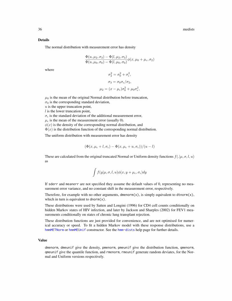
The normal distribution with measurement error has density

Φ(u, µ2, σ3)− Φ(l, µ2, σ3)

Φ(u, µ0, σ0)− Φ(l, µ0, σ0)φ(x, µ0 + µε, σ2)

whereσ22 = σ2

0 + σ2ε ,

σ3 = σ0σε/σ2,

µ2 = (x− µε)σ20 + µ0σ

2ε ,

µ0 is the mean of the original Normal distribution before truncation,σ0 is the corresponding standard deviation,u is the upper truncation point,l is the lower truncation point,σε is the standard deviation of the additional measurement error,µε is the mean of the measurement error (usually 0).φ(x) is the density of the corresponding normal distribution, andΦ(x) is the distribution function of the corresponding normal distribution.

The uniform distribution with measurement error has density

(Φ(x, µε + l, σε)− Φ(x, µε + u, σε))/(u− l)

These are calculated from the original truncated Normal or Uniform density functions f(.|µ, σ, l, u)as ∫

f(y|µ, σ, l, u)φ(x, y + µε, σε)dy

If sderr and meanerr are not specified they assume the default values of 0, representing no mea-surement error variance, and no constant shift in the measurement error, respectively.

Therefore, for example with no other arguments, dmenorm(x), is simply equivalent to dtnorm(x),which in turn is equivalent to dnorm(x).

These distributions were used by Satten and Longini (1996) for CD4 cell counts conditionally onhidden Markov states of HIV infection, and later by Jackson and Sharples (2002) for FEV1 mea-surements conditionally on states of chronic lung transplant rejection.

These distribution functions are just provided for convenience, and are not optimised for numer-ical accuracy or speed. To fit a hidden Markov model with these response distributions, use ahmmMETNorm or hmmMEUnif constructor. See the hmm-dists help page for further details.

Value

dmenorm, dmeunif give the density, pmenorm, pmeunif give the distribution function, qmenorm,qmeunif give the quantile function, and rmenorm, rmeunif generate random deviates, for the Nor-mal and Uniform versions respectively.

model.frame.msm 37

Author(s)


References

Satten, G.A. and Longini, I.M. Markov chains with measurement error: estimating the ’true’ courseof a marker of the progression of human immunodeficiency virus disease (with discussion) AppliedStatistics 45(3): 275-309 (1996)


See Also

dnorm, dunif, dtnorm

Examples

## what does the distribution look like?x <- seq(50, 90, by=1)plot(x, dnorm(x, 70, 10), type="l", ylim=c(0,0.06)) ## standard Normallines(x, dtnorm(x, 70, 10, 60, 80), type="l") ## truncated Normal## truncated Normal with small measurement errorlines(x, dmenorm(x, 70, 10, 60, 80, sderr=3), type="l")

model.frame.msm Extract original data from msm objects.

Description

Extract the data from a multi-state model fitted with msm.

Usage

## S3 method for class 'msm'model.frame(formula, agg=FALSE, ...)## S3 method for class 'msm'model.matrix(object, model="intens", state=1, ...)

Arguments

formula A fitted multi-state model object, as returned by msm.

agg Return the model frame in the efficient aggregated form used to calculate thelikelihood internally for non-hidden Markov models. This has one row for eachunique combination of from-state, to-state, time lag, covariate value and obser-vation type. The variable named "(nocc)" counts how many observations ofthat combination there are in the original data.

38 msm


model "intens" to return the design matrix for covariates on intensities, "misc" formisclassification probabilities, "hmm" for a general hidden Markov model, and"inits" for initial state probabilities in hidden Markov models.

state State corresponding to the required covariate design matrix in a hidden Markovmodel.

... Further arguments (not used).

Value

model.frame returns a data frame with all the original variables used for the model fit, with anymissing data removed (see na.action in msm). The state, time, subject, obstype and obstruevariables are named "(state)", "(time)", "(subject)", "(obstype)" and "(obstrue)" respec-tively (note the brackets). A variable called "(obs)" is the observation number from the originaldata before any missing data were dropped. The variable "(pcomb)" is used for computing thelikelihood for hidden Markov models, and identifies which distinct time difference, obstype andcovariate values (thus which distinct interval transition probability matrix) each observation corre-sponds to.

The model frame object has some other useful attributes, including "usernames" giving the user’soriginal names for these variables (used for model refitting, e.g. in bootstrapping or cross validation)and "covnames" identifying which ones are covariates.

model.matrix returns a design matrix for a part of the model that includes covariates. The requiredpart is indicated by the "model" argument.

For time-inhomogeneous models fitted with "pci", these datasets will have imputed observationsat each time change point, indicated where the variable "(pci.imp)" in the model frame is 1. Themodel matrix for intensities will have factor contrasts for the timeperiod covariate.

Author(s)


See Also

msm, model.frame, model.matrix.

msm Multi-state Markov and hidden Markov models in continuous time

Description

Fit a continuous-time Markov or hidden Markov multi-state model by maximum likelihood. Obser-vations of the process can be made at arbitrary times, or the exact times of transition between statescan be known. Covariates can be fitted to the Markov chain transition intensities or to the hiddenMarkov observation process.

msm 39

Usage

msm ( formula, subject=NULL, data = list(), qmatrix, gen.inits = FALSE,ematrix=NULL, hmodel=NULL, obstype=NULL, obstrue=NULL,covariates = NULL, covinits = NULL, constraint = NULL,misccovariates = NULL, misccovinits = NULL, miscconstraint = NULL,hcovariates = NULL, hcovinits = NULL, hconstraint = NULL, hranges=NULL,qconstraint=NULL, econstraint=NULL, initprobs = NULL,est.initprobs=FALSE, initcovariates = NULL, initcovinits = NULL,deathexact = NULL, death=NULL, exacttimes = FALSE, censor=NULL,censor.states=NULL, pci=NULL, phase.states=NULL, phase.inits=NULL,cl = 0.95, fixedpars = NULL, center=TRUE,opt.method="optim", hessian=NULL, use.deriv=TRUE,use.expm=TRUE, analyticp=TRUE, na.action=na.omit, ... )

Arguments


Observed states should be numeric variables in the set 1, ..., n, wheren is the number of states. Factors are allowed only if their levels are called"1", ..., "n".The times can indicate different types of observation scheme, so be careful tochoose the correct obstype.For hidden Markov models, state refers to the outcome variable, which neednot be a discrete state. It may also be a matrix, giving multiple observations ateach time (see hmmMV).


data Optional data frame in which to interpret the variables supplied in formula,subject, covariates, misccovariates, hcovariates, obstype and obstrue.

qmatrix Matrix which indicates the allowed transitions in the continuous-time Markovchain, and optionally also the initial values of those transitions. If an instanta-neous transition is not allowed from state r to state s, then qmatrix should have(r, s) entry 0, otherwise it should be non-zero.If supplying initial values yourself, then the non-zero entries should be thosevalues. If using gen.inits=TRUE then the non-zero entries can be anythingyou like (conventionally 1). Any diagonal entry of qmatrix is ignored, as it isconstrained to be equal to minus the sum of the rest of the row.For example,

rbind( c( 0, 0.1, 0.01 ), c( 0.1, 0, 0.2 ), c( 0, 0, 0 ))

40 msm

represents a ’health - disease - death’ model, with initial transition intensities0.1 from health to disease, 0.01 from health to death, 0.1 from disease to health,and 0.2 from disease to death.If the states represent ordered levels of severity of a disease, then this matrixshould usually only allow transitions between adjacent states. For example, ifsomeone was observed in state 1 ("mild") at their first observation, followed bystate 3 ("severe") at their second observation, they are assumed to have passedthrough state 2 ("moderate") in between, and the 1,3 entry of qmatrix shouldbe zero.The initial intensities given here are with any covariates set to their means in thedata (or set to zero, if center = FALSE). If any intensities are constrainedto be equal using qconstraint, then the initial value is taken from the first ofthese (reading across rows).

gen.inits If TRUE, then initial values for the transition intensities are generated automati-cally using the method in crudeinits.msm. The non-zero entries of the suppliedqmatrix are assumed to indicate the allowed transitions of the model. This isnot available for hidden Markov models, including models with misclassifiedstates.

ematrix If misclassification between states is to be modelled, this should be a matrix ofinitial values for the misclassification probabilities. The rows represent underly-ing states, and the columns represent observed states. If an observation of states is not possible when the subject occupies underlying state r, then ematrixshould have (r, s) entry 0. Otherwise ematrix should have (r, s) entry corre-sponding to the probability of observing s conditionally on occupying true stater. The diagonal of ematrix is ignored, as rows are constrained to sum to 1. Forexample,

rbind( c( 0, 0.1, 0 ), c( 0.1, 0, 0.1 ), c( 0, 0.1, 0 ))

represents a model in which misclassifications are only permitted between adja-cent states.If any probabilities are constrained to be equal using econstraint, then theinitial value is taken from the first of these (reading across rows).For an alternative way of specifying misclassification models, see hmodel.

hmodel Specification of the hidden Markov model (HMM). This should be a list of re-turn values from HMM constructor functions. Each element of the list corre-sponds to the outcome model conditionally on the corresponding underlyingstate. Univariate constructors are described in thehmm-dists help page. Thesemay also be grouped together to specify a multivariate HMM with a set of con-ditionally independent univariate outcomes at each time, as described in hmmMV.For example, consider a three-state hidden Markov model. Suppose the ob-servations in underlying state 1 are generated from a Normal distribution withmean 100 and standard deviation 16, while observations in underlying state 2are Normal with mean 54 and standard deviation 18. Observations in state 3,representing death, are exactly observed, and coded as 999 in the data. Thismodel is specified as

msm 41

hmodel = list(hmmNorm(mean=100, sd=16), hmmNorm(mean=54, sd=18), hmmIdent(999))

The mean and standard deviation parameters are estimated starting from theseinitial values. If multiple parameters are constrained to be equal using hconstraint,then the initial value is taken from the value given on the first occasion that pa-rameter appears in hmodel.See the hmm-dists help page for details of the constructor functions for eachunivariate distribution.A misclassification model, that is, a hidden Markov model where the outcomesare misclassified observations of the underlying states, can either be specifiedusing a list of hmmCat or hmmIdent objects, or by using an ematrix.For example,

ematrix = rbind( c( 0, 0.1, 0, 0 ), c( 0.1, 0, 0.1, 0 ), c( 0, 0.1, 0, 0), c( 0, 0, 0, 0))

is equivalent to

hmodel = list( hmmCat(prob=c(0.9, 0.1, 0, 0)), hmmCat(prob=c(0.1, 0.8, 0.1, 0)), hmmCat(prob=c(0, 0.1, 0.9, 0)), hmmIdent())

obstype A vector specifying the observation scheme for each row of the data. This canbe included in the data frame data along with the state, time, subject IDs andcovariates. Its elements should be either 1, 2 or 3, meaning as follows:

1 An observation of the process at an arbitrary time (a "snapshot" of the process,or "panel-observed" data). The states are unknown between observationtimes.

2 An exact transition time, with the state at the previous observation retaineduntil the current observation. An observation may represent a transition toa different state or a repeated observation of the same state (e.g. at the endof follow-up). Note that if all transition times are known, more flexiblemodels could be fitted with packages other than msm - see the note underexacttimes.Note also that if the previous state was censored using censor, for exampleknown only to be state 1 or state 2, then obstype 2 means that either state1 is retained or state 2 is retained until the current observation - this doesnot allow for a change of state in the middle of the observation interval.

3 An exact transition time, but the state at the instant before entering this state isunknown. A common example is death times in studies of chronic diseases.

If obstype is not specified, this defaults to all 1. If obstype is a single number,all observations are assumed to be of this type. The obstype value for the firstobservation from each subject is not used.This is a generalisation of the deathexact and exacttimes arguments to allowdifferent schemes per observation. obstype overrides both deathexact andexacttimes.exacttimes=TRUE specifies that all observations are of obstype 2.

42 msm

deathexact = death.states specifies that all observations of death.statesare of type 3. deathexact = TRUE specifies that all observations in thefinal absorbing state are of type 3.

obstrue In misclassification models specified with ematrix, obstrue is a vector of logi-cals (TRUE or FALSE) or numerics (1 or 0) specifying which observations (TRUE,1) are observations of the underlying state without error, and which (FALSE, 0)are realisations of a hidden Markov model.In HMMs specified with hmodel, where the hidden state is known at some times,if obstrue is supplied it is assumed to contain the actual true state data. Ele-ments of obstrue at times when the hidden state is unknown are set to NA.This allows the information from HMM outcomes generated conditionally onthe known state to be included in the model, thus improving the estimation ofthe HMM outcome distributions.In HMMs where there are also censored states, obstrue should be set to 1 forobserved states which are censored but not misclassified.

covariates A formula or a list of formulae representing the covariates on the transitionintensities via a log-linear model. If a single formula is supplied, likecovariates = ~ age + sex + treatment

then these covariates are assumed to apply to all intensities. If a named list issupplied, then this defines a potentially different model for each named intensity.For example,covariates = list("1-2" = ~ age, "2-3" = ~ age + treatment)

specifies an age effect on the state 1 - state 2 transition, additive age and treat-ment effects on the state 2 - state 3 transition, but no covariates on any othertransitions that are allowed by the qmatrix.If covariates are time dependent, they are assumed to be constant in between thetimes they are observed, and the transition probability between a pair of times(t1, t2) is assumed to depend on the covariate value at t1.

covinits Initial values for log-linear effects of covariates on the transition intensities. Thisshould be a named list with each element corresponding to a covariate. A singleelement contains the initial values for that covariate on each transition intensity,reading across the rows in order. For a pair of effects constrained to be equal,the initial value for the first of the two effects is used.For example, for a model with the above qmatrix and age and sex covariates, thefollowing initialises all covariate effects to zero apart from the age effect on the2-1 transition, and the sex effect on the 1-3 transition. covinits = list(sex=c(0, 0, 0.1, 0), age=c(0, 0.1, 0, 0))

For factor covariates, name each level by concatenating the name of the covariatewith the level name, quoting if necessary. For example, for a covariate agegroupwith three levels 0-15, 15-60, 60-, use something likecovinits = list("agegroup15-60"=c(0, 0.1, 0, 0), "agegroup60-"=c(0.1, 0.1, 0, 0))

If not specified or wrongly specified, initial values are assumed to be zero.

constraint A list of one numeric vector for each named covariate. The vector indicateswhich covariate effects on intensities are constrained to be equal. Take, for ex-ample, a model with five transition intensities and two covariates. Specifying

msm 43

constraint = list (age = c(1,1,1,2,2), treatment = c(1,2,3,4,5))

constrains the effect of age to be equal for the first three intensities, and equalfor the fourth and fifth. The effect of treatment is assumed to be different foreach intensity. Any vector of increasing numbers can be used as indicators. Theintensity parameters are assumed to be ordered by reading across the rows of thetransition matrix, starting at the first row, ignoring the diagonals.Negative elements of the vector can be used to indicate that particular covariateeffects are constrained to be equal to minus some other effects. For example:constraint = list (age = c(-1,1,1,2,-2), treatment = c(1,2,3,4,5))

constrains the second and third age effects to be equal, the first effect to be minusthe second, and the fifth age effect to be minus the fourth. For example, it may berealisitic that the effect of a covariate on the "reverse" transition rate from state2 to state 1 is minus the effect on the "forward" transition rate, state 1 to state2. Note that it is not possible to specify exactly which of the covariate effectsare constrained to be positive and which negative. The maximum likelihoodestimation chooses the combination of signs which has the higher likelihood.For categorical covariates, defined as factors, specify constraints as follows:

list(..., covnameVALUE1 = c(...), covnameVALUE2 = c(...), ...)

where covname is the name of the factor, and VALUE1, VALUE2, ... are the labelsof the factor levels (usually excluding the baseline, if using the default contrasts).Make sure the contrasts option is set appropriately, for example, the defaultoptions(contrasts=c(contr.treatment, contr.poly))

sets the first (baseline) level of unordered factors to zero, then the baseline levelis ignored in this specification.To assume no covariate effect on a certain transition, use the fixedpars argu-ment to fix it at its initial value (which is zero by default) during the optimisation.

misccovariates A formula representing the covariates on the misclassification probabilities, anal-ogously to covariates, via multinomial logistic regression. Only used if themodel is specified using ematrix, rather than hmodel.This must be a single formula - lists are not supported, unlike covariates. Ifa different model on each probability is required, include all covariates in thisformula, and use fixedpars to fix some of their effects (for particular probabil-ities) at their default initial values of zero.

misccovinits Initial values for the covariates on the misclassification probabilities, defined inthe same way as covinits. Only used if the model is specified using ematrix.

miscconstraint A list of one vector for each named covariate on misclassification probabilities.The vector indicates which covariate effects on misclassification probabilitiesare constrained to be equal, analogously to constraint. Only used if the modelis specified using ematrix.

hcovariates List of formulae the same length as hmodel, defining any covariates governingthe hidden Markov outcome models. The covariates operate on a suitably link-transformed linear scale, for example, log scale for a Poisson outcome model. If

44 msm

there are no covariates for a certain hidden state, then insert a NULL in the corre-sponding place in the list. For example, hcovariates = list(~acute + age, ~acute, NULL).

hcovinits Initial values for the hidden Markov model covariate effects. A list of the samelength as hcovariates. Each element is a vector with initial values for the ef-fect of each covariate on that state. For example, the above hcovariates canbe initialised with hcovariates = list(c(-8, 0), -8, NULL). Initial valuesmust be given for all or no covariates, if none are given these are all set to zero.The initial value given in the hmodel constructor function for the correspondingbaseline parameter is interpreted as the value of that parameter with any covari-ates fixed to their means in the data. If multiple effects are constrained to beequal using hconstraint, then the initial value is taken from the first of themultiple initial values supplied.

hconstraint A named list. Each element is a vector of constraints on the named hiddenMarkov model parameter. The vector has length equal to the number of timesthat class of parameter appears in the whole model.For example consider the three-state hidden Markov model described above,with normally-distributed outcomes for states 1 and 2. To constrain the outcomevariance to be equal for states 1 and 2, and to also constrain the effect of acuteon the outcome mean to be equal for states 1 and 2, specifyhconstraint = list(sd = c(1,1), acute=c(1,1))

Note this excludes initial state occupancy probabilities and covariate effects onthose probabilities, which cannot be constrained.

hranges Range constraints for hidden Markov model parameters. Supplied as a namedlist, with each element corresponding to the named hidden Markov model pa-rameter. This element is itself a list with two elements, vectors named "lower"and "upper". These vectors each have length equal to the number of timesthat class of parameter appears in the whole model, and give the correspond-ing mininum amd maximum allowable values for that parameter. Maximumlikelihood estimation is performed with these parameters constrained in theseranges (through a log or logit-type transformation). Lower bounds of -Inf andupper bounds of Inf can be given if the parameter is unbounded above or below.For example, in the three-state model above, to constrain the mean for state 1 tobe between 0 and 6, and the mean of state 2 to be between 7 and 12, supplyhranges=list(mean=list(lower=c(0, 7), upper=c(6, 12)))

These default to the natural ranges, e.g. the positive real line for variance pa-rameters, and [0,1] for probabilities. Therefore hranges need not be specifiedfor such parameters unless an even stricter constraint is desired. If only onelimit is supplied for a parameter, only the first occurrence of that parameter isconstrained.Initial values should be strictly within any ranges, and not on the range boundary,otherwise optimisation will fail with a "non-finite value" error.

qconstraint A vector of indicators specifying which baseline transition intensities are equal.For example,qconstraint = c(1,2,3,3)

constrains the third and fourth intensities to be equal, in a model with four al-lowed instantaneous transitions. When there are covariates on the intensities

msm 45

and center=TRUE (the default), qconstraint is applied to the intensities withcovariates taking the values of the means in the data. When center=FALSE,qconstraint is applied to the intensities with covariates set to zero.

econstraint A similar vector of indicators specifying which baseline misclassification prob-abilities are constrained to be equal. Only used if the model is specified usingematrix, rather than hmodel.

initprobs Only used in hidden Markov models. Underlying state occupancy probabilitiesat each subject’s first observation. Can either be a vector of nstates elementswith common probabilities to all subjects, or a nsubjects by nstates matrix ofsubject-specific probabilities. This refers to observations after missing data andsubjects with only one observation have been excluded.If these are estimated (see est.initprobs), then this represents an initial value,and defaults to equal probability for each state. Otherwise this defaults to c(1, rep(0, nstates-1)),that is, in state 1 with a probability of 1. Scaled to sum to 1 if necessary. Thestate 1 occupancy probability should be non-zero.

est.initprobs Only used in hidden Markov models. If TRUE, then the underlying state occu-pancy probabilities at the first observation will be estimated, starting from a vec-tor of initial values supplied in the initprobs argument. Structural zeroes areallowed: if any of these initial values are zero they will be fixed at zero duringoptimisation, even if est.initprobs=TRUE, and no covariate effects on themare estimated. The exception is state 1, which should have non-zero occupancyprobability.Note that the free parameters during this estimation exclude the state 1 occu-pancy probability, which is fixed at one minus the sum of the other probabilities.

initcovariates Formula representing covariates on the initial state occupancy probabilities, viamultinomial logistic regression. The linear effects of these covariates, observedat the individual’s first observation time, operate on the log ratio of the state roccupancy probability to the state 1 occupancy probability, for each r = 2 to thenumber of states. Thus the state 1 occupancy probability should be non-zero.If est.initprobs is TRUE, these effects are estimated starting from their initialvalues. If est.initprobs is FALSE, these effects are fixed at theit initial values.

initcovinits Initial values for the covariate effects initcovariates. A named list with eachelement corresponding to a covariate, as in covinits. Each element is a vectorwith (1 - number of states) elements, containing the initial values for the lineareffect of that covariate on the log odds of that state relative to state 1, from state2 to the final state. If initcovinits is not specified, all covariate effects areinitialised to zero.

deathexact Vector of indices of absorbing states whose time of entry is known exactly, butthe individual is assumed to be in an unknown transient state ("alive") at theprevious instant. This is the usual situation for times of death in chronic diseasemonitoring data. For example, if you specify deathexact = c(4, 5) thenstates 4 and 5 are assumed to be exactly-observed death states.See the obstype argument. States of this kind correspond to obstype=3. deathexact = TRUEindicates that the final absorbing state is of this kind, and deathexact = FALSEor deathexact = NULL (the default) indicates that there is no state of this kind.The deathexact argument is overridden by obstype or exacttimes.

46 msm

Note that you do not always supply a deathexact argument, even if there arestates that correspond to deaths, because they do not necessarily have obstype=3.If the state is known between the time of death and the previous observation,then you should specify obstype=2 for the death times, or exacttimes=TRUE ifthe state is known at all times, and the deathexact argument is ignored.

death Old name for the deathexact argument. Overridden by deathexact if both aresupplied. Deprecated.

censor A state, or vector of states, which indicates censoring. Censoring means that theobserved state is known only to be one of a particular set of states. For exam-ple, censor=999 indicates that all observations of 999 in the vector of observedstates are censored states. By default, this means that the true state could havebeen any of the transient (non-absorbing) states. To specify corresponding truestates explicitly, use a censor.states argument.Note that in contrast to the usual terminology of survival analysis, here it is thestate which is considered to be censored, rather than the event time. If at the endof a study, an individual has not died, but their true state is known, then censor isunnecessary, since the standard multi-state model likelihood is applicable. Alsoa "censored" state here can be at any time, not just at the end.Note in particular that general time-inhomogeneous Markov models with piece-wise constant transition intensities can be constructed using the censor facility.If the true state is unknown on occasions when a piecewise constant covariateis known to change, then censored states can be inserted in the data on thoseoccasions. The covariate may represent time itself, in which case the pci optionto msm can be used to perform this trick automatically, or some other time-dependent variable.

censor.states Specifies the underlying states which censored observations can represent. Ifcensor is a single number (the default) this can be a vector, or a list with oneelement. If censor is a vector with more than one element, this should be a list,with each element a vector corresponding to the equivalent element of censor.For examplecensor = c(99, 999), censor.states = list(c(2,3), c(3,4))

means that observations coded 99 represent either state 2 or state 3, while obser-vations coded 999 are really either state 3 or state 4.

pci Model for piecewise-constant intensities. Vector of cut points defining the times,since the start of the process, at which intensities change for all subjects. Forexamplepci = c(5, 10)

specifies that the intensity changes at time points 5 and 10. This will automati-cally construct a model with a categorical (factor) covariate called timeperiod,with levels "[-Inf,5)", "[5,10)" and "[10,Inf)", where the first level is thebaseline. This covariate defines the time period in which the observation wasmade. Initial values and constraints on covariate effects are specified the sameway as for a model with a covariate of this name, for example,covinits = list("timeperiod[5,10)"=c(0.1,0.1), "timeperiod[10,Inf)"=c(0.1,0.1))

Thus if pci is supplied, you cannot have a previously-existing variable calledtimeperiod as a covariate in any part of a msm model.

msm 47

To assume piecewise constant intensities for some transitions but not others withpci, use the fixedpars argument to fix the appropriate covariate effects at theirdefault initial values of zero.Internally, this works by inserting censored observations in the data at timeswhen the intensity changes but the state is not observed.If the supplied times are outside the range of the time variable in the data, pciis ignored and a time-homogeneous model is fitted.After fitting a time-inhomogeneous model, qmatrix.msm can be used to obtainthe fitted intensity matrices for each time period, for example,qmatrix.msm(example.msm, covariates=list(timeperiod="[5,Inf)"))

This facility does not support interactions between time and other covariates.Such models need to be specified "by hand", using a state variable with censoredobservations inserted. Note that the data component of the msm object returnedfrom a call to msm with pci supplied contains the states with inserted censoredobservations and time period indicators. These can be used to construct suchmodels.Note that you do not need to use pci in order to model the effect of a time-dependent covariate in the data. msm will automatically assume that covariatesare piecewise-constant and change at the times when they are observed. pci isfor when you want all intensities to change at the same pre-specified times forall subjects.

phase.states Indices of states which have a two-phase sojourn distribution. This defines asemi-Markov model, in which the hazard of an onward transition depends onthe time spent in the state.This uses the technique described by Titman and Sharples (2009). A hiddenMarkov model is automatically constructed on an expanded state space, wherethe phases correspond to the hidden states. The "tau" proportionality constraintdescribed in this paper is currently not supported.Covariates, constraints, deathexact and censor are expressed with respect tothe expanded state space. If not supplied by hand, initprobs is defined auto-matically so that subjects are assumed to begin in the first of the two phases.Hidden Markov models can additionally be given phased states. The user sup-plies an outcome distribution for each original state using hmodel, which is ex-panded internally so that it is assumed to be the same within each of the phasedstates. initprobs is interpreted on the expanded state space. Misclassificationmodels defined using ematrix are not supported, and these must be defined us-ing hmmCat or hmmIdent constructors, as described in the hmodel section of thishelp page. Or the HMM on the expanded state space can be defined by hand.Output functions are presented as it were a hidden Markov model on the ex-panded state space, for example, transition probabilities between states, covari-ate effects on transition rates, or prevalence counts, are not aggregated over thehidden phases.Numerical estimation will be unstable when there is weak evidence for a two-phase sojourn distribution, that is, if the model is close to Markov.See d2phase for the definition of the two-phase distribution and the interpreta-tion of its parameters.

48 msm

This is an experimental feature, and some functions are not implemented. Pleasereport any experiences of using this feature to the author!

phase.inits Initial values for phase-type models. A list with one component for each "two-phased" state. Each component is itself a list of two elements. The first of theseelements is a scalar defining the transition intensity from phase 1 to phase 2.The second element is a matrix, with one row for each potential destination statefrom the two-phased state, and two columns. The first column is the transitionrate from phase 1 to the destination state, and the second column is the transitionrate from phase 2 to the destination state. If there is only one destination state,then this may be supplied as a vector.In phase type models, the initial values for transition rates out of non-phasedstates are taken from the qmatrix supplied to msm, and entries of this matrixcorresponding to transitions out of phased states are ignored.

exacttimes By default, the transitions of the Markov process are assumed to take place atunknown occasions in between the observation times. If exacttimes is set toTRUE, then the observation times are assumed to represent the exact times oftransition of the process. The subject is assumed to be in the same state betweenthese times. An observation may represent a transition to a different state ora repeated observation of the same state (e.g. at the end of follow-up). Thisis equivalent to every row of the data having obstype = 2. See the obstypeargument. If both obstype and exacttimes are specified then exacttimes isignored.Note that the complete history of the multi-state process is known with this typeof data. The models which msm fits have the strong assumption of constant (orpiecewise-constant) transition rates. Knowing the exact transition times allowsmore realistic models to be fitted with other packages. For example parametricmodels with sojourn distributions more flexible than the exponential can be fittedwith the flexsurv package, or semi-parametric models can be implemented withsurvival in conjunction with mstate.

cl Width of symmetric confidence intervals for maximum likelihood estimates, bydefault 0.95.

fixedpars Vector of indices of parameters whose values will be fixed at their initial val-ues during the optimisation. These are given in the order: transition inten-sities (reading across rows of the transition matrix), covariates on intensities(ordered by intensities within covariates), hidden Markov model parameters,including misclassification probabilities (ordered by parameters within states),hidden Markov model covariate parameters (ordered by covariates within pa-rameters within states), initial state occupancy probabilities (excluding the firstprobability, which is fixed at one minus the sum of the others).If there are equality constraints on certain parameters, then fixedpars indexesthe set of unique parameters, excluding those which are constrained to be equalto previous parameters.To fix all parameters, specify fixedpars = TRUE.This can be useful for profiling likelihoods, and building complex models stageby stage.

center If TRUE (the default, unless fixedpars=TRUE) then covariates are centered at

msm 49

their means during the maximum likelihood estimation. This usually improvesstability of the numerical optimisation.

opt.method If "optim", "nlm" or "bobyqa", then the corresponding R function will be usedfor maximum likelihood estimation. optim is the default. "bobyqa" requiresthe package minqa to be installed. See the help of these functions for furtherdetails. Advanced users can also add their own optimisation methods, see thesource for optim.R in msm for some examples.If "fisher", then a specialised Fisher scoring method is used (Kalbfleisch andLawless, 1985) which can be faster than the generic methods, though less robust.This is only available for Markov models with panel data (obstype=1), that is,not for models with censored states, hidden Markov models, exact observationor exact death times (obstype=2,3).

hessian If TRUE then standard errors and confidence intervals are obtained from a nu-merical estimate of the Hessian (the observed information matrix). This is thedefault when maximum likelihood estimation is performed. If all parameters arefixed at their initial values and no optimisation is performed, then this defaults toFALSE. If requested, the actual Hessian is returned in x$paramdata$opt$hessian,where x is the fitted model object.If hessian is set to FALSE, then standard errors and confidence intervals areobtained from the Fisher (expected) information matrix, if this is available. Thismay be preferable if the numerical estimation of the Hessian is computationallyintensive, or if the resulting estimate is non-invertible or not positive definite.

use.deriv If TRUE then analytic first derivatives are used in the optimisation of the like-lihood, where available and an appropriate quasi-Newton optimisation method,such as BFGS, is being used. Analytic derivatives are not available for all mod-els.

use.expm If TRUE then any matrix exponentiation needed to calculate the likelihood is doneusing the expm package. Otherwise the original routines used in msm 1.2.4 andearlier are used. Set to FALSE for backward compatibility, and let the packagemaintainer know if this gives any substantive differences.

analyticp By default, the likelihood for certain simpler 3, 4 and 5 state models is cal-culated using an analytic expression for the transition probability (P) matrix.For all other models, matrix exponentiation is used to obtain P. To revert tothe original method of using the matrix exponential for all models, specifyanalyticp=FALSE. See the PDF manual for a list of the models for which ana-lytic P matrices are implemented.

na.action What to do with missing data: either na.omit to drop it and carry on, or na.failto stop with an error. Missing data includes all NAs in the states, times, subjector obstrue, all NAs at the first observation for a subject for covariates in initcovariates,all NAs in other covariates (excluding the last observation for a subject), all NAsin obstype (excluding the first observation for a subject), and any subjects withonly one observation (thus no observed transitions).

... Optional arguments to the general-purpose R optimisation routine, optim bydefault. For example method="Nelder-Mead" to change the optimisation algo-rithm from the "BFGS" method that msm calls by default.It is often worthwhile to normalize the optimisation using control=list(fnscale = a),where a is the a number of the order of magnitude of the -2 log likelihood.

50 msm

If ’false’ convergence is reported and the standard errors cannot be calculateddue to a non-positive-definite Hessian, then consider tightening the tolerancecriteria for convergence. If the optimisation takes a long time, intermediatesteps can be printed using the trace argument of the control list. See optim fordetails.For the Fisher scoring method, a control list can be supplied in the same way,but the only supported options are reltol, trace and damp. The first two areused in the same way as for optim. If the algorithm fails with a singular in-formation matrix, adjust damp from the default of zero (to, e.g. 1). This addsa constant identity matrix multiplied by damp to the information matrix duringoptimisation.

Details

For full details about the methodology behind the msm package, refer to the PDF manual ‘msm-manual.pdf’in the ‘doc’ subdirectory of the package. This includes a tutorial in the typical use of msm. Thepaper by Jackson (2011) in Journal of Statistical Software presents the material in this manual in amore concise form.

msm was designed for fitting continuous-time Markov models, processes where transitions can oc-cur at any time. These models are defined by intensities, which govern both the time spent in thecurrent state and the probabilities of the next state. In discrete-time models, transitions are knownin advance to only occur at multiples of some time unit, and the model is purely governed by theprobability distributions of the state at the next time point, conditionally on the state at the currenttime. These can also be fitted in msm, assuming that there is a continuous-time process under-lying the data. Then the fitted transition probability matrix over one time period, as returned bypmatrix.msm(...,t=1) is equivalent to the matrix that governs the discrete-time model. How-ever, these can be fitted more efficiently using multinomial logistic regression, for example, usingmultinom from the R package nnet (Venables and Ripley, 2002).

For simple continuous-time multi-state Markov models, the likelihood is calculated in terms ofthe transition intensity matrix Q. When the data consist of observations of the Markov process atarbitrary times, the exact transition times are not known. Then the likelihood is calculated usingthe transition probability matrix P (t) = exp(tQ), where exp is the matrix exponential. If state iis observed at time t and state j is observed at time u, then the contribution to the likelihood fromthis pair of observations is the i, j element of P (u− t). See, for example, Kalbfleisch and Lawless(1985), Kay (1986), or Gentleman et al. (1994).

For hidden Markov models, the likelihood for an individual with k observations is calculated di-rectly by summing over the unknown state at each time, producing a product of k matrices. Thecalculation is a generalisation of the method described by Satten and Longini (1996), and also byJackson and Sharples (2002), and Jackson et al. (2003).

There must be enough information in the data on each state to estimate each transition rate, other-wise the likelihood will be flat and the maximum will not be found. It may be appropriate to reducethe number of states in the model, the number of allowed transitions, or the number of covariate ef-fects, to ensure convergence. Hidden Markov models, and situations where the value of the processis only known at a series of snapshots, are particularly susceptible to non-identifiability, especiallywhen combined with a complex transition matrix. Choosing an appropriate set of initial values forthe optimisation can also be important. For flat likelihoods, ’informative’ initial values will oftenbe required. See the PDF manual for other tips.

msm 51

Value

To obtain summary information from models fitted by the msm function, it is recommended to useextractor functions such as qmatrix.msm, pmatrix.msm, sojourn.msm, msm.form.qoutput. Theseprovide estimates and confidence intervals for quantities such as transition probabilities for givencovariate values.

For advanced use, it may be necessary to directly use information stored in the object returned bymsm. This is documented in the help page msm.object.

Printing a msm object by typing the object’s name at the command line implicitly invokes print.msm.This formats and prints the important information in the model fit, and also returns that informationin an R object. This includes estimates and confidence intervals for the transition intensities and(log) hazard ratios for the corresponding covariates. When there is a hidden Markov model, thechief information in the hmodel component is also formatted and printed. This includes estimatesand confidence intervals for each parameter.

Author(s)


References

Jackson, C.H. (2011). Multi-State Models for Panel Data: The msm Package for R., Journal ofStatistical Software, 38(8), 1-29. URL http://www.jstatsoft.org/v38/i08/.

Kalbfleisch, J., Lawless, J.F., The analysis of panel data under a Markov assumption Journal of theAmerical Statistical Association (1985) 80(392): 863–871.

Kay, R. A Markov model for analysing cancer markers and disease states in survival studies. Bio-metrics (1986) 42: 855–865.

Gentleman, R.C., Lawless, J.F., Lindsey, J.C. and Yan, P. Multi-state Markov models for analysingincomplete disease history data with illustrations for HIV disease. Statistics in Medicine (1994)13(3): 805–821.

Satten, G.A. and Longini, I.M. Markov chains with measurement error: estimating the ’true’ courseof a marker of the progression of human immunodeficiency virus disease (with discussion) AppliedStatistics 45(3): 275-309 (1996)


Jackson, C.H., Sharples, L.D., Thompson, S.G. and Duffy, S.W. and Couto, E. Multi-state Markovmodels for disease progression with classification error. The Statistician, 52(2): 193–209 (2003)

Titman, A.C. and Sharples, L.D. Semi-Markov models with phase-type sojourn distributions. Bio-metrics 66, 742-752 (2009).

Venables, W.N. and Ripley, B.D. (2002) Modern Applied Statistics with S, second edition. Springer.

See Also

simmulti.msm, plot.msm, summary.msm, qmatrix.msm, pmatrix.msm, sojourn.msm.

52 msm.form.qoutput

Examples

### Heart transplant data### For further details and background to this example, see### Jackson (2011) or the PDF manual in the doc directory.print(cav[1:10,])twoway4.q <- rbind(c(-0.5, 0.25, 0, 0.25), c(0.166, -0.498, 0.166, 0.166),c(0, 0.25, -0.5, 0.25), c(0, 0, 0, 0))statetable.msm(state, PTNUM, data=cav)crudeinits.msm(state ~ years, PTNUM, data=cav, qmatrix=twoway4.q)cav.msm <- msm( state ~ years, subject=PTNUM, data = cav,

qmatrix = twoway4.q, deathexact = 4,control = list ( trace = 2, REPORT = 1 ) )

cav.msmqmatrix.msm(cav.msm)pmatrix.msm(cav.msm, t=10)sojourn.msm(cav.msm)

msm.form.qoutput Extract msm model parameter estimates in compact format

Description

Extract estimates and confidence intervals for transition intensities (or misclassification probabili-ties), and their covariate effects, in a tidy matrix format with one row per transition. This is usedby the print method (print.msm) for msm objects. Covariate effects are returned as hazard or oddsratios, not on the log scale.

Usage

msm.form.qoutput(x, covariates="mean", cl=0.95, digits=4, ...)msm.form.eoutput(x, covariates="mean", cl=0.95, digits=4, ...)

Arguments

x A fitted multi-state model object, as returned by msm.

covariates Covariate values defining the "baseline" parameters (see qmatrix.msm).


digits Minimum number of significant digits for the formatted character matrix re-turned as an attribute. This is passed to format. Defaults to 4.

... Other arguments to be passed to format.

Value

A numeric matrix with one row per transition, and one column for each estimate or confidence limit.The "formatted" attribute contains the same results formatted for pretty printing. msm.form.qoutputreturns the transition intensities and their covariates, and msm.form.eoutput returns the misclassi-fication probabilities and their covariates.

msm.object 53

Author(s)


See Also

print.msm

msm.object Fitted msm model objects

Description

The msm function returns a list with the following components. These are intended for developersand confident users. To extract results from fitted model objects, functions such as qmatrix.msm orprint.msm should be used instead.

Value

call The original call to msm, as returned by match.call.

Qmatrices A list of matrices. The first component, labelled logbaseline, is a matrix con-taining the estimated transition intensities on the log scale with any covariatesfixed at their means in the data (or at zero, if center=FALSE). The componentlabelled baseline is the equivalent on the untransformed scale. Each remain-ing component is a matrix giving the linear effects of the labelled covariate onthe matrix of log intensities. To extract an estimated intensity matrix on thenatural scale, at an arbitrary combination of covariate values, use the functionqmatrix.msm.

QmatricesSE The standard error matrices corresponding to Qmatrices.QmatricesL,QmatricesU

Corresponding lower and upper symmetric confidence limits, of width 0.95 un-less specified otherwise by the cl argument.

Ematrices A list of matrices. The first component, labelled logitbaseline, is the esti-mated misclassification probability matrix (expressed as as log odds relative tothe probability of the true state) with any covariates fixed at their means in thedata (or at zero, if center=FALSE). The component labelled baseline is theequivalent on the untransformed scale. Each remaining component is a matrixgiving the linear effects of the labelled covariate on the matrix of logit mis-classification probabilities. To extract an estimated misclassification probabilitymatrix on the natural scale, at an arbitrary combination of covariate values, usethe function ematrix.msm.

EmatricesSE The standard error matrices corresponding to Ematrices.EmatricesL,EmatricesU

Corresponding lower and upper symmetric confidence limits, of width 0.95 un-less specified otherwise by the cl argument.

minus2loglik Minus twice the maximised log-likelihood.

54 msm.object

deriv Derivatives of the minus twice log-likelihood at its maximum.

estimates Vector of untransformed maximum likelihood estimates returned from optim.Transition intensities are on the log scale and misclassification probabilities aregiven as log odds relative to the probability of the true state.

estimates.t Vector of transformed maximum likelihood estimates with intensities and prob-abilities on their natural scales.

fixedpars Indices of estimates which were fixed during the maximum likelihood estima-tion.

center Indicator for whether the estimation was performed with covariates centered ontheir means in the data.

covmat Covariance matrix corresponding to estimates.

ci Matrix of confidence intervals corresponding to estimates.t

opt Return value from the optimisation routine (such as optim or nlm), giving infor-mation about the results of the optimisation.

foundse Logical value indicating whether the Hessian was positive-definite at the sup-posed maximum of the likelihood. If not, the covariance matrix of the parame-ters is unavailable. In these cases the optimisation has probably not convergedto a maximum.

data A list giving the data used for the model fit, for use in post-processing. To extractit, use the methods model.frame.msm or model.matrix.msm.The format of this element changed in version 1.4 of msm, so that it now con-tains a model.frame object mf with all the variables used in the model. Theprevious format (an ad-hoc list of vectors and matrices) can be obtained withthe function recreate.olddata(msmobject), where msmobject is the objectreturned by msm.

qmodel A list of objects representing the transition matrix structure and options for like-lihood calculation. See qmodel.object for documentation of the components.

emodel A list of objects representing the misclassification model structure, for modelsspecified using the ematrix argument to msm. See emodel.object.

qcmodel A list of objects representing the model for covariates on transition intensities.See qcmodel.object.

ecmodel A list of objects representing the model for covariates on transition intensities.See ecmodel.object.

hmodel A list of objects representing the hidden Markov model structure. See hmodel.object.

cmodel A list giving information about censored states. See cmodel.object.

pci Cut points for time-varying intensities, as supplied to msm, but excluding anythat are outside the times observed in the data.

paramdata A list giving information about the parameters of the multi-state model. Seeparamdata.object.

cl Confidence interval width, as supplied to msm.

covariates Formula for covariates on intensities, as supplied to msm.

misccovariates Formula for covariates on misclassification probabilities, as supplied to msm.

msm.summary 55

hcovariates Formula for covariates on hidden Markov model outcomes, as supplied to msm.

initcovariates Formula for covariates on initial state occupancy probabilities in hidden Markovmodels, as supplied to msm.

sojourn A list as returned by sojourn.msm, with components:mean = estimated mean sojourn times in the transient states, with covariates fixedat their means (if center=TRUE) or at zero (if center=FALSE).se = corresponding standard errors.

msm.summary Summarise a fitted multi-state model

Description

Summary method for fitted msm models. This is simply a wrapper around prevalence.msm whichproduces a table of observed and expected state prevalences for each time, and for models withcovariates, hazard.msm to print hazard ratios with 95% confidence intervals for covariate effects.

Usage

## S3 method for class 'msm'summary(object, hazard.scale=1, ...)

Arguments


hazard.scale Vector with same elements as number of covariates on transition rates. Corre-sponds to the increase in each covariate used to calculate its hazard ratio. De-faults to all 1.

... Further arguments passed to prevalence.msm.

Value

A list of class summary.msm, with components:

prevalences Output from prevalence.msm.

hazard Output from hazard.msm.

hazard.scale Value of the hazard.scale argument.

Author(s)


See Also

msm,prevalence.msm, hazard.msm

56 msm2Surv

msm2Surv Convert data for ‘msm’ to data for ‘survival’, ‘mstate’ or ‘flexsurv’analysis

Description

Converts longitudinal data for a msm model fit, where observations represent the exact transitiontimes of the process, to counting process data. This enables, for example, flexible parametric multi-state models to be fitted with flexsurvreg from the flexsurv package, or semiparametric modelsto be implemented with coxph and the mstate package.

Usage

msm2Surv(data, subject, time, state, covs, Q)

Arguments

data Data frame in the format expected by a msm model fit with exacttimes=TRUE orall obstype=2. Each row represents an observation of a state, and the time vari-able contains the exact and complete transition times of the underlying process.This is explained in more detail in the help page for msm, section obstype=2.

subject Name of the subject ID in the data (character format, i.e. quoted).

time Name of the time variable in the data (character).

state Name of the state variable in the data (character).

covs Vector of covariate names to carry through (character). If not supplied, this istaken to be all remaining variables in the data.

Q Transition intensity matrix. This should have number of rows and number ofcolumns both equal to the number of states. If an instantaneous transition is notallowed from state r to state s, then Q should have (r, s) entry 0, otherwise itshould be non-zero. The diagonal entries are ignored.

Details

For example, if the data supplied to msm look like this:

subj days status age treat1 0 1 66 11 27 2 66 11 75 3 66 11 97 4 66 11 1106 4 69 12 0 1 49 02 90 2 49 02 1037 2 51 0

msm2Surv 57

then the output of msm2Surv will be a data frame looking like this:

id from to Tstart Tstop time status age treat trans1 1 2 0 27 27 1 66 1 11 1 4 0 27 27 0 66 1 21 2 3 27 75 48 1 66 1 31 2 4 27 75 48 0 66 1 41 3 4 75 97 22 1 69 1 52 1 2 0 90 90 1 49 0 12 1 4 0 90 90 0 49 0 22 2 3 90 1037 947 0 49 0 32 2 4 90 1037 947 0 49 0 4

At 27 days, subject 1 is observed to move from state 1 to state 2 (first row, status 1), which meansthat their potential transition from state 1 to state 4 is censored (second row, status 0).

See the mstate package and the references below for more details of this data format and using itfor semi-parametric multi-state modelling.

Value

A data frame of class "msdata", with rows representing observed or censored transitions. Therewill be one row for each observed transition in the original data, and additional rows for everypotential transition that could have occurred out of each observed state.

The data frame will have columns called:

id Subject ID

from Starting state of the transition

to Finishing state of the transition

Tstart The starting time of the transition

Tstop The finishing time of the transition

time The time difference = Tstop - Tstart

status Event or censoring indicator, with 1 indicating an observed transition, and 0indicating censoring

trans Transition number

and any remaining columns will represent covariates. Any covariates whose names clash withthe standard variables in the returned data ("id", "from", "to", "Tstart", "Tstop", "time","status" or "trans") have ".2" appended to their names.

The transition matrix in mstate format is stored in the trans attribute of the returned object. Seethe example code below.

Author(s)


58 odds.msm

References

Putter H, Fiocco M, Geskus RB (2007). Tutorial in biostatistics: Competing risks and multi-statemodels. Statistics in Medicine 26: 2389-2430.

Liesbeth C. de Wreede, Marta Fiocco, Hein Putter (2011). mstate: An R Package for the Analysisof Competing Risks and Multi-State Models. Journal of Statistical Software, 38(7), 1-30. http://www.jstatsoft.org/v38/i07

Jackson, C. H. (2014). flexsurv: Flexible parametric survival and multi-state models. R packageversion 0.5.

See Also

msprep, in mstate, which produces data in a similar format, given data in "wide" format with onerow per subject.

Examples

msmdat <- data.frame(subj = c(1, 1, 1, 1, 1, 2, 2, 2),days = c(0, 27, 75, 97, 1106, 0, 90, 1037),status = c(1, 2, 3, 4, 4, 1, 2, 2),age = c(66, 66, 66, 66, 69, 49, 49, 51),treat = c(1, 1, 1, 1, 1, 0, 0, 0))# transitions only allowed to next state up or state 4Q <- rbind(c(1, 1, 0, 1),

c(0, 1, 1, 1),c(0, 0, 1, 1),c(0, 0, 0, 0))

dat <- msm2Surv(data=msmdat, subject="subj", time="days", state="status",Q=Q)

datattr(dat, "trans")

odds.msm Calculate tables of odds ratios for covariates on misclassificationprobabilities

Description

Odds ratios are computed by exponentiating the estimated covariate effects on the logit-misclassificationprobabilities.

Usage

odds.msm(x, odds.scale = 1, cl = 0.95)

http://www.jstatsoft.org/v38/i07

http://www.jstatsoft.org/v38/i07

paramdata.object 59

Arguments

x Output from msm representing a fitted multi-state model.

odds.scale Vector with same elements as number of covariates on misclassification proba-bilities. Corresponds to the increase in each covariate used to calculate its oddsratio. Defaults to all 1.


Value

A list of tables containing odds ratio estimates, one table for each covariate. Each table has threecolumns, containing the odds ratio, and an approximate upper 95% and lower 95% confidence limitrespectively (assuming normality on the log scale), for each misclassification probability.

Author(s)


See Also

msm, hazard.msm

paramdata.object Developer documentation: internal msm parameters object

Description

An object giving information about the parameters of the multi-state model. Used internally duringmaximum likelihood estimation and arranging results. Returned as the paramdata component of afitted msm model object.

Value

inits Vector of initial values for distinct parameters which are being estimated. Thesehave been transformed to the real line (e.g. by log), and exclude parametersbeing fixed at their initial values, parameters defined to be always fixed (e.g.binomial denominators) and parameters constrained to equal previous ones.

plabs Names of parameters in allinits.

allinits Vector of parameter values before estimation, including those which are fixed orconstrained to equal other parameters, and transformed to the real line.

hmmpars Indices of allinits which represent baseline parameters of hidden Markov out-come models (thus excluding covariate effects in HMMs and initial state occu-pancy probabilities).

fixed TRUE if all parameters are fixed, FALSE otherwise.

60 paramdata.object

fixedpars Indices of parameters in allinits which are fixed, either by definition or asrequested by the user in the fixedpars argument to msm. Excludes parametersfixed by constraining to equal other parameters.

notfixed Indices of parameters which are not fixed by the definition of fixedpars.

optpars Indices of parameters in allinits being estimated, thus those included in inits.

auxpars Indices of "auxiliary" parameters which are always fixed, for example, binomialdenominators (hmmBinom) and the which parameter in hmmIdent.

constr Vector of integers, of length npars, indicating which sets of parameters are con-strained to be equal to each other. If two of these integers are equal the corre-sponding parameters are equal. A negative element indicates that parameter isdefined to be minus some other parameter (this is used for covariate effects ontransition intensities).

npars Total number of parameters, equal to length(allinits).

nfix Number of fixed parameters, equal to length(fixedpars).

nopt Number of parameters being estimated, equal to length(inits) and length(optpars).

ndup Number of parameters defined as duplicates of previous parameters by equalityconstraints (currently unused).

ranges Matrix of defined ranges for each parameter on the natural scale (e.g. 0 to infin-ity for rate parameters).

opt Object returned by the optimisation routine (such as optim).

foundse TRUE if standard errors are available after optimisation. If FALSE the optimisationprobably hasn’t converged.

lik Minus twice the log likelihood at the parameter estimates.

deriv Derivatives of the minus twice log likelihood at the parameter estimates, if avail-able.

information Corresponding expected information matrix at the parameter estimates, if avail-able.

params Vector of parameter values after maximum likelihood estimation, correspondingto allinits, still on the real-line transformed scale.

covmat Covariance matrix corresponding to params.

ci Matrix of confidence intervals corresponding to params, with nominal coverage(default 0.95) defined by the cl argument of msm.

estimates.t Vector of parameter estimates, as params but with parameters on their naturalscales.

See Also

msm.object

pearson.msm 61

pearson.msm Pearson-type goodness-of-fit test

Description

Pearson-type goodness-of-fit test for multi-state models fitted to panel-observed data.

Usage

pearson.msm(x, transitions=NULL, timegroups=3, intervalgroups=3,covgroups=3, groups=NULL, boot=FALSE, B=500,next.obstime=NULL, N=100, indep.cens=TRUE,maxtimes=NULL, pval=TRUE)

Arguments


transitions This should be an integer vector indicating which interval transitions shouldbe grouped together in the contingency table. Its length should be the numberof allowed interval transitions, excluding transitions from absorbing states toabsorbing states.The allowed interval transitions are the set of pairs of states (a, b) for which itis possible to observe a at one time and b at any later time. For example, ina "well-disease-death" model with allowed instantaneous 1-2, 2-3 transitions,there are 5 allowed interval transitions. In numerical order, these are 1-1, 1-2,1-3, 2-2 and 2-3, excluding absorbing-absorbing transitions.Then, to group transitions 1-1,1-2 together, and transitions 2-2,2-3 together,specifytransitions = c(1,1,2,3,3).Only transitions from the same state may be grouped. By default, each intervaltransition forms a separate group.

timegroups Number of groups based on quantiles of the time since the start of the process.

intervalgroups Number of groups based on quantiles of the time interval between observations,within time groups

covgroups Number of groups based on quantiles of∑r qirr, where qirr are the diagonal

entries of the transition intensity matrix for the ith transition. These are a func-tion of the covariate effects and the covariate values at the ith transition: qirr isminus the sum of the off-diagonal entries q(0)rs exp(βTrszi) on the rth row.Thus covgroups summarises the impact of covariates at each observation, bycalculating the overall rate of progression through states at that observation.For time-inhomogeneous models specified using the pci argument to msm, ifthe only covariate is the time period, covgroups is set to 1, since timegroupsensures that transitions are grouped by time.

62 pearson.msm

groups A vector of arbitrary groups in which to categorise each transition. This canbe an integer vector or a factor. This can be used to diagnose specific areasof poor fit. For example, the contingency table might be grouped by arbitrarycombinations of covariates to detect types of individual for whom the model fitspoorly.The length of groups should be x$data$n, the number of observations used inthe model fit, which is the number of observations in the original dataset withany missing values excluded. The value of groups at observation i is used tocategorise the transition which ends at observation i. Values of groups at thefirst observation for each subject are ignored.

boot Estimate an "exact" p-value using a parametric bootstrap.All objects used in the original call to msm which produced x, such as the qmatrix,should be in the working environment, or else an “object not found” error willbe given. This enables the original model to be refitted to the replicate datasets.Note that groups cannot be used with bootstrapping, as the simulated observa-tions will not be in the same categories as the original observations.


next.obstime This is a vector of length x$data$n (the number of observations used in themodel fit) giving the time to the next scheduled observation following each timepoint. This is only used when times to death are known exactly.For individuals who died (entered an absorbing state) before the next scheduledobservation, and the time of death is known exactly, next.obstime would begreater than the observed death time.If the individual did not die, and a scheduled observation did follow that timepoint, next.obstime should just be the same as the time to that observation.next.obstime is used to determine a grouping of the time interval betweenobservations, which should be based on scheduled observations. If exact timesto death were used in the grouping, then shorter intervals would contain excessdeaths, and the goodness-of-fit statistic would be biased.If next.obstime is unknown, it is multiply-imputed using a product-limit es-timate based on the intervals to observations other than deaths. The resultingtables of transitions are averaged over these imputations. This may be slow.

N Number of imputations for the estimation of the distribution of the next sched-uled observation time, when there are exact death times.

indep.cens If TRUE, then times to censoring are included in the estimation of the distributionto the next scheduled observation time. If FALSE, times to censoring are assumedto be systematically different from other observation times.

maxtimes A vector of length x$data$n, or a common scalar, giving an upper bound for thenext scheduled observation time. Used in the multiple imputation when timesto death are known exactly. If a value greater than maxtimes is simulated, thenthe next scheduled observation is taken as censored. This should be supplied, ifknown. If not supplied, this is taken to be the maximum interval occurring inthe data, plus one time unit. For observations which are not exact death times,this should be the time since the previous observation.

pval Calculate a p-value using the improved approximation of Titman (2009). Thisis optional since it is not needed during bootstrapping, and it is computationally

pearson.msm 63

non-trivial. Only available currently for non-hidden Markov models for paneldata without exact death times. Also not available for models with censoring,including time-homogeneous models fitted with the pci option to msm.

Details

This method (Aguirre-Hernandez and Farewell, 2002) is intended for data which represent observa-tions of the process at arbitrary times ("snapshots", or "panel-observed" data). For data which rep-resent the exact transition times of the process, prevalence.msm can be used to assess fit, thoughwithout a formal test.

When times of death are known exactly, states are misclassified, or an individual’s final observationis a censored state, the modification by Titman and Sharples (2008) is used. The only form ofcensoring supported is a state at the end of an individual’s series which represents an unknowntransient state (i.e. the individual is only known to be alive at this time). Other types of censoringare omitted from the data before performing the test.

See the references for further details of the methods. The method used for censored states is amodification of the method in the appendix to Titman and Sharples (2008), described at http://www.mrc-bsu.cam.ac.uk/wp-content/uploads/robustcensoring.pdf (Titman, 2007).

Groupings of the time since initiation, the time interval and the impact of covariates are based onequally-spaced quantiles. The number of groups should be chosen that there are not many cellswith small expected numbers of transitions, since the deviance statistic will be unstable for sparsecontingency tables. Ideally, the expected numbers of transitions in each cell of the table shouldbe no less than about 5. Conversely, the power of the test is reduced if there are too few groups.Therefore, some sensitivity analysis of the test results to the grouping is advisable.

Saved model objects fitted with previous versions of R (versions less than 1.2) will need to berefitted under the current R for use with pearson.msm.

Value

A list whose first two elements are contingency tables of observed transitions O and expected tran-sitionsE, respectively, for each combination of groups. The third element is a table of the deviances(O−E)2/E multiplied by the sign of O−E. If the expected number of transitions is zero then thedeviance is zero. Entries in the third matrix will be bigger in magnitude for groups for which themodel fits poorly.

"test" the fourth element of the list, is a data frame with one row containing thePearson-type goodness-of-fit test statistic stat. The test statistic is the sumof the deviances. For panel-observed data without exact death times, misclassi-fication or censored observations, p is the p-value for the test statistic calculatedusing the improved approximation of Titman (2009).For these models, for comparison with older versions of the package, test alsopresents p.lower and p.upper, which are theoretical lower and upper limitsfor the p-value of the test statistic, based on χ2 distributions with df.lowerand df.upper degrees of freedom, respectively. df.upper is the number ofindependent cells in the contingency table, and df.lower is df.upper minusthe number of estimated parameters in the model.

http://www.mrc-bsu.cam.ac.uk/wp-content/uploads/robustcensoring.pdf

http://www.mrc-bsu.cam.ac.uk/wp-content/uploads/robustcensoring.pdf

64 pearson.msm

"intervalq" (not printed by default) contains the definition of the grouping of the intervalsbetween observations. These groups are defined by quantiles within the groupscorresponding to the time since the start of the process.

"sim" If there are exact death times, this contains simulations of the contingency ta-bles and test statistics for each imputation of the next scheduled sampling time.These are averaged over to produce the presented tables and test statistic. Thiselement is not printed by default.With exact death times, the null variance of the test statistic (formed by takingmean of simulated test statistics) is less than twice the mean (Titman, 2008), andthe null distribution is not χ2. In this case, p.upper is an upper limit for the trueasymptotic p-value, but p.lower is not a lower limit, and is not presented.

"boot" If the bootstrap has been used, the element will contain the bootstrap replicatesof the test statistics (not printed by default).

"lambda" If the Titman (2009) p-value has been calculated, this contains the weights defin-ing the null distribution of the test statistic as a weighted sum of χ2

1 randomvariables (not printed by default).

Author(s)

Andrew Titman <[email protected]>, Chris Jackson <[email protected]>

References

Aguirre-Hernandez, R. and Farewell, V. (2002) A Pearson-type goodness-of-fit test for stationaryand time-continuous Markov regression models. Statistics in Medicine 21:1899-1911.

Titman, A. and Sharples, L. (2008) A general goodness-of-fit test for Markov and hidden Markovmodels. Statistics in Medicine 27(12):2177-2195

Titman, A. (2009) Computation of the asymptotic null distribution of goodness-of-fit tests for multi-state models. Lifetime Data Analysis 15(4):519-533.

Titman, A. (2008) Model diagnostics in multi-state models of biological systems. PhD thesis,University of Cambridge.

See Also

msm, prevalence.msm, scoreresid.msm,

Examples

psor.q <- rbind(c(0,0.1,0,0),c(0,0,0.1,0),c(0,0,0,0.1),c(0,0,0,0))psor.msm <- msm(state ~ months, subject=ptnum, data=psor,

qmatrix = psor.q, covariates = ~ollwsdrt+hieffusn,constraint = list(hieffusn=c(1,1,1),ollwsdrt=c(1,1,2)))

pearson.msm(psor.msm, timegroups=2, intervalgroups=2, covgroups=2)# More 1-2, 1-3 and 1-4 observations than expected in shorter time# intervals - the model fits poorly.# A random effects model might accommodate such fast progressors.

pexp 65

pexp Exponential distribution with piecewise-constant rate

Description

Density, distribution function, quantile function and random generation for a generalisation of theexponential distribution, in which the rate changes at a series of times.

Usage

dpexp(x, rate=1, t=0, log = FALSE)ppexp(q, rate=1, t=0, lower.tail = TRUE, log.p = FALSE)qpexp(p, rate=1, t=0, lower.tail = TRUE, log.p = FALSE)rpexp(n, rate=1, t=0)

Arguments




rate vector of rates.

t vector of the same length as rate, giving the times at which the rate changes.The first element of t should be 0, and t should be in increasing order.

log, log.p logical; if TRUE, probabilities p are given as log(p), or log density is returned.


Details

Consider the exponential distribution with rates r1, . . . , rn changing at times t1, . . . , tn, with t1 =0. Suppose tk is the maximum ti such that ti < x. The density of this distribution at x > 0 is f(x)for k = 1, and

k∏i=1

(1− F (ti − ti−1, ri))f(x− tk, rk)

for k > 1.

whereF () and f() are the distribution and density functions of the standard exponential distribution.

If rate is of length 1, this is just the standard exponential distribution. Therefore, for example,dpexp(x), with no other arguments, is simply equivalent to dexp(x).

Only rpexp is used in the msm package, to simulate from Markov processes with piecewise-constantintensities depending on time-dependent covariates. These functions are merely provided for com-pletion, and are not optimized for numerical stability or speed.

66 phasemeans.msm

Value

dpexp gives the density, ppexp gives the distribution function, qpexp gives the quantile function,and rpexp generates random deviates.

Author(s)


See Also

dexp, sim.msm.

Examples

x <- seq(0.1, 50, by=0.1)rate <- c(0.1, 0.2, 0.05, 0.3)t <- c(0, 10, 20, 30)## standard exponential distributionplot(x, dexp(x, 0.1), type="l")## distribution with piecewise constant ratelines(x, dpexp(x, rate, t), type="l", lty=2)## standard exponential distributionplot(x, pexp(x, 0.1), type="l")## distribution with piecewise constant ratelines(x, ppexp(x, rate, t), type="l", lty=2)

phasemeans.msm Parameters of phase-type models in mixture form

Description

Parameters of fitted two-phase models, in mixture model parameterisation.

Usage

phasemeans.msm(x, covariates="mean", ci=c("none","normal","bootstrap"),cl=0.95, B=1000, cores=NULL)

Arguments

x A fitted multi-state model, as returned by msm.covariates Covariate values, see qmatrix.msm.ci If "none" (the default) no confidence intervals are calculated. Otherwise "normal",

or "boot" as described by qmatrix.msm.cl Width of the symmetric confidence interval, relative to 1.B Number of bootstrap replicates, or number of normal simulations from the dis-

tribution of the MLEs.cores Number of cores to use for bootstrapping using parallel processing. See boot.msm

for more details.

plot.msm 67

Value

Matrix with one row for each state that has a two-phase distribution, and three columns: the short-stay mean, long-stay mean and long-stay probability. These are functions of the transition intensitiesof the expanded hidden Markov model, defined in d2phase.

Author(s)


See Also

d2phase.

plot.msm Plots of multi-state models

Description

This produces a plot of the expected probability of survival against time, from each transient state.Survival is defined as not entering an absorbing state.

Usage

## S3 method for class 'msm'plot(x, from, to, range, covariates, legend.pos, xlab="Time",

ylab="Fitted survival probability", lwd=1, ...)

Arguments

x Output from msm, representing a fitted multi-state model object.from States from which to consider survival. Defaults to the complete set of transient

states.to Absorbing state to consider. Defaults to the highest-labelled absorbing state.range Vector of two elements, giving the range of times to plot for.covariates Covariate values for which to evaluate the expected probabilities. This can ei-

ther be:





68 plot.prevalence.msm

legend.pos Vector of the x and y position, respectively, of the legend.

xlab x axis label.

ylab y axis label.

lwd Line width. See par.

... Other arguments to be passed to the generic plot and lines functions.

Author(s)


See Also

msm

plot.prevalence.msm Plot of observed and expected prevalences

Description

Provides a rough indication of goodness of fit of a multi-state model, by estimating the observednumbers of individuals occupying a state at a series of times, and plotting these against forecastsfrom the fitted model, for each state. Observed prevalences are indicated as solid lines, expectedprevalences as dashed lines.

Usage

## S3 method for class 'prevalence.msm'plot(x, mintime=NULL, maxtime=NULL, timezero=NULL,

initstates=NULL, interp=c("start","midpoint"),censtime=Inf, subset=NULL,covariates="population", misccovariates="mean",piecewise.times=NULL, piecewise.covariates=NULL,xlab="Times",ylab="Prevalence (%)", lwd.obs=1,lwd.exp=1, lty.obs=1, lty.exp=2, col.obs="blue",col.exp="red", legend.pos=NULL,...)

Arguments

x A fitted multi-state model produced by msm.

mintime Minimum time at which to compute the observed and expected prevalences ofstates.

maxtime Maximum time at which to compute the observed and expected prevalences ofstates.

timezero Initial time of the Markov process. Expected values are forecasted from here.Defaults to the minimum of the observation times given in the data.

plot.prevalence.msm 69

initstates Optional vector of the same length as the number of states. Gives the numbersof individuals occupying each state at the initial time, to be used for forecastingexpected prevalences. The default is those observed in the data. These shouldadd up to the actual number of people in the study at the start.

interp Interpolation method for observed states, see prevalence.msm.

censtime Subject-specific maximum follow-up times, see prevalence.msm.

subset Vector of the subject identifiers to calculated observed prevalences for.

covariates Covariate values for which to forecast expected state occupancy. See prevalence.msm— if this function runs too slowly, as it may if there are continuous covariates,replace covariates="population" with covariates="mean".

misccovariates (Misclassification models only) Values of covariates on the misclassificationprobability matrix. See prevalence.msm.

piecewise.times

Times at which piecewise-constant intensities change. See prevalence.msm.piecewise.covariates

Covariates on which the piecewise-constant intensities depend. See prevalence.msm.

xlab x axis label.

ylab y axis label.

lwd.obs Line width for observed prevalences. See par.

lwd.exp Line width for expected prevalences. See par.

lty.obs Line type for observed prevalences. See par.

lty.exp Line type for expected prevalences. See par.

col.obs Line colour for observed prevalences. See par.

col.exp Line colour for expected prevalences. See par.


... Further arguments to be passed to the generic plot function.

Details

See prevalence.msm for details of the assumptions underlying this method.

Observed prevalences are plotted with a solid line, and expected prevalences with a dotted line.

References


See Also

prevalence.msm

70 plot.survfit.msm

plot.survfit.msm Plot empirical and fitted survival curves

Description

Plot a Kaplan-Meier estimate of the survival probability and compare it with the fitted survivalprobability from a msm model.

Usage

## S3 method for class 'survfit.msm'plot(x, from=1, to=NULL, range=NULL, covariates="mean",

interp=c("start","midpoint"), ci=c("none","normal","bootstrap"), B=100,legend.pos=NULL, xlab="Time", ylab="Survival probability",lty=1, lwd=1, col="red", lty.ci=2, lwd.ci=1, col.ci="red",mark.time=TRUE, col.surv="blue", lty.surv=2, lwd.surv=1,survdata=FALSE,...)

Arguments

x Output from msm, representing a fitted multi-state model object.

from Non-absorbing state from which to consider survival. Defaults to state 1. Thefitted probabilities will then be calculated as the transition probabilities from thisstate to to. The empirical survival curve plots survival from the first observationof from (where this exists) to the first entry time into to.

to Absorbing state to consider. Defaults to the highest-labelled absorbing state.

range Vector of two elements, giving the range of times to plot for.

covariates Covariate values for which to evaluate the expected probabilities. This can ei-ther be:





but note the empirical curve is plotted for the full population. To consider sub-sets for the empirical curve, set survdata=TRUE to extract the survival data andbuild a survival plot by hand using plot.survfit.

plot.survfit.msm 71

ci If "none" (the default) no confidence intervals are plotted. If "normal" or"bootstrap", confidence intervals are plotted based on the respective methodin pmatrix.msm. This is very computationally-intensive, since intervals must becomputed at a series of times.

B Number of bootstrap or normal replicates for the confidence interval. The de-fault is 100 rather than the usual 1000, since these plots are for rough diagnosticpurposes.

interp If interp="start" (the default) then the entry time into the absorbing state isassumed to be the time it is first observed in the data.If interp="midpoint" then the entry time into the absorbing state is assumedto be halfway between the time it is first observed and the previous observationtime. This is generally more reasonable for "progressive" models with observa-tions at arbitrary times.


xlab x axis label.

ylab y axis label.

lty Line type for the fitted curve. See par.

lwd Line width for the fitted curve. See par.

col Colour for the fitted curve. See par.

lty.ci Line type for the fitted curve confidence limits. See par.

lwd.ci Line width for the fitted curve confidence limits. See par.

col.ci Colour for the fitted curve confidence limits. See par.

mark.time Mark the empirical survival curve at each censoring point, see lines.survfit.

col.surv Colour for the empirical survival curve, passed to lines.survfit. See par.

lty.surv Line type for the empirical survival curve, passed to lines.survfit. See par.

lwd.surv Line width for the empirical survival curve, passed to lines.survfit. See par.

survdata Set to TRUE to return the survival data frame constructed when plotting the em-pirical curve. This can be used for constructing survival plots by hand usingplot.survfit.

... Other arguments to be passed to the plot function which draws the fitted curve,or the lines.survfit function which draws the empirical curve.

Details

If the data represent observations of the process at arbitrary times, then the first occurrence of theabsorbing state in the data will usually be greater than the actual first transition time to that state.Therefore the Kaplan-Meier estimate of the survival probability will be an overestimate.

The method of Turnbull (1976) could be used to give a non-parametric estimate of the time to aninterval-censored event, and compared to the equivalent estimate from a multi-state model. This isimplemented in the CRAN package interval (Fay and Shaw 2010).

This currently only handles time-homogeneous models.

72 plotprog.msm

References

Turnbull, B. W. (1976) The empirical distribution function with arbitrarily grouped, censored andtruncated data. J. R. Statist. Soc. B 38, 290-295.

Fay, MP and Shaw, PA (2010). Exact and Asymptotic Weighted Logrank Tests for Interval CensoredData: The interval R package. Journal of Statistical Software. http://www.jstatsoft.org/v36/ i02/.36 (2):1-34.

See Also

survfit, plot.survfit, plot.prevalence.msm

plotprog.msm Kaplan Meier estimates of incidence

Description

Compute and plot Kaplan-Meier estimates of the probability that each successive state has notoccurred yet.

Usage

plotprog.msm(formula, subject, data, legend.pos=NULL, xlab="Time",ylab="1 - incidence probability", lwd=1, xlim=NULL,mark.time=TRUE, ...)

Arguments


Observed states should be in the set 1, ..., n, where n is the number of states.


data An optional data frame in which the variables represented by state, time andsubject can be found.


xlab x axis label.

ylab y axis label.

lwd Line width. See par.

xlim x axis limits, e.g. c(0,10) for an axis ranging from 0 to 10. Default is the rangeof observation times.

mark.time Mark the empirical survival curve at each censoring point, see lines.survfit.

... Other arguments to be passed to the plot and lines.survfit functions.

pmatrix.msm 73

Details

If the data represent observations of the process at arbitrary times, then the first occurrence of thestate in the data will usually be greater than the actual first transition time to that state. Thereforethe probabilities plotted by plotprog.msm will be overestimates.

See Also

survfit, plot.survfit

pmatrix.msm Transition probability matrix

Description

Extract the estimated transition probability matrix from a fitted multi-state model for a given timeinterval, at a given set of covariate values.

Usage

pmatrix.msm(x=NULL, t=1, t1=0, covariates="mean",ci=c("none","normal","bootstrap"), cl=0.95, B=1000,cores=NULL, qmatrix=NULL,...)

Arguments


t The time interval to estimate the transition probabilities for, by default one unit.

t1 The starting time of the interval. Used for models x with piecewise-constantintensities fitted using the pci option to msm. The probabilities will be computedon the interval [t1, t1+t].

covariates The covariate values at which to estimate the transition probabilities. This caneither be:





If some covariates are specified but not others, the missing ones default to zero.

74 pmatrix.msm

For time-inhomogeneous models fitted using the pci option to msm, "covariates"here include only those specified using the covariates argument to msm, andexclude the artificial covariates representing the time period.For time-inhomogeneous models fitted "by hand" by using a time-dependent co-variate in the covariates argument to msm, the function pmatrix.piecewise.msmshould be used to to calculate transition probabilities.

ci If "normal", then calculate a confidence interval for the transition probabilitiesby simulating B random vectors from the asymptotic multivariate normal distri-bution implied by the maximum likelihood estimates (and covariance matrix) ofthe log transition intensities and covariate effects, then calculating the resultingtransition probability matrix for each replicate. See, e.g. Mandel (2013) for adiscussion of this approach.If "bootstrap" then calculate a confidence interval by non-parametric bootstraprefitting. This is 1-2 orders of magnitude slower than the "normal" method, butis expected to be more accurate. See boot.msm for more details of bootstrappingin msm.If "none" (the default) then no confidence interval is calculated.

cl Width of the symmetric confidence interval, relative to 1.B Number of bootstrap replicates, or number of normal simulations from the dis-

tribution of the MLEscores Number of cores to use for bootstrapping using parallel processing. See boot.msm

for more details.qmatrix A transition intensity matrix. Either this or a fitted model x must be supplied.

No confidence intervals are available if qmatrix is supplied.... Optional arguments to be passed to MatrixExp to control the method of com-

puting the matrix exponential.

Details

For a continuous-time homogeneous Markov process with transition intensity matrix Q, the proba-bility of occupying state s at time u+ t conditionally on occupying state r at time u is given by the(r, s) entry of the matrix P (t) = exp(tQ), where exp() is the matrix exponential.

For non-homogeneous processes, where covariates and hence the transition intensity matrix Q arepiecewise-constant in time, the transition probability matrix is calculated as a product of matricesover a series of intervals, as explained in pmatrix.piecewise.msm.

The pmatrix.piecewise.msm function is only necessary for models fitted using a time-dependentcovariate in the covariates argument to msm. For time-inhomogeneous models fitted using "pci",pmatrix.msm can be used, with arguments t and t1, to calculate transition probabilities over anytime period.

Value

The matrix of estimated transition probabilities P (t) in the given time. Rows correspond to "from-state" and columns to "to-state".

Or if ci="normal" or ci="bootstrap", pmatrix.msm returns a list with components estimatesand ci, where estimates is the matrix of estimated transition probabilities, and ci is a list of twomatrices containing the upper and lower confidence limits.

pmatrix.piecewise.msm 75

Author(s)

C. H. Jackson <[email protected]>.

References

Mandel, M. (2013). "Simulation based confidence intervals for functions with complicated deriva-tives." The American Statistician 67(2):76-81

See Also

qmatrix.msm, pmatrix.piecewise.msm, boot.msm

pmatrix.piecewise.msm Transition probability matrix for processes with piecewise-constant in-tensities

Description

Extract the estimated transition probability matrix from a fitted non-time-homogeneous multi-statemodel for a given time interval. This is a generalisation of pmatrix.msm to models with time-dependent covariates. Note that pmatrix.msm is sufficient to calculate transition probabilities fortime-inhomogeneous models fitted using the pci argument to msm.

Usage

pmatrix.piecewise.msm(x=NULL, t1, t2, times, covariates,ci=c("none","normal","bootstrap"), cl=0.95, B=1000, cores=NULL,qlist=NULL,...)

Arguments

x A fitted multi-state model, as returned by msm. This should be a non-homogeneousmodel, whose transition intensity matrix depends on a time-dependent covariate.

t1 The start of the time interval to estimate the transition probabilities for.

t2 The end of the time interval to estimate the transition probabilities for.

times Cut points at which the transition intensity matrix changes.

covariates A list with number of components one greater than the length of times. Eachcomponent of the list is specified in the same way as the covariates argumentto pmatrix.msm. The components correspond to the covariate values in theintervals(t1, times[1]], (times[1], times[2]], ..., (times[length(times)], t2]

(assuming that all elements of times are in the interval (t1, t2)).

76 pmatrix.piecewise.msm

ci If "normal", then calculate a confidence interval for the transition probabilitiesby simulating B random vectors from the asymptotic multivariate normal distri-bution implied by the maximum likelihood estimates (and covariance matrix) ofthe log transition intensities and covariate effects, then calculating the resultingtransition probability matrix for each replicate.If "bootstrap" then calculate a confidence interval by non-parametric bootstraprefitting. This is 1-2 orders of magnitude slower than the "normal" method, butis expected to be more accurate. See boot.msm for more details of bootstrappingin msm.If "none" (the default) then no confidence interval is calculated.




qlist A list of transition intensity matrices, of length one greater than the length oftimes. Either this or a fitted model x must be supplied. No confidence intervalsare available if (just) qlist is supplied.

... Optional arguments to be passed to MatrixExp to control the method of com-puting the matrix exponential.

Details

Suppose a multi-state model has been fitted, in which the transition intensity matrixQ(x(t)) is mod-elled in terms of time-dependent covariates x(t). The transition probability matrix P (t1, tn) for thetime interval (t1, tn) cannot be calculated from the estimated intensity matrix as exp((tn − t1)Q),because Q varies within the interval t1, tn. However, if the covariates are piecewise-constant, orcan be approximated as piecewise-constant, then we can calculate P (t1, tn) by multiplying togetherindividual matrices P (ti, ti+1) = exp((ti+1− ti)Q), calculated over intervals where Q is constant:

P (t1, tn) = P (t1, t2)P (t2, t3) . . . P (tn−1, tn)

Value

The matrix of estimated transition probabilities P (t) for the time interval [t1, tn]. That is, theprobabilities of occupying state s at time tn conditionally on occupying state r at time t1. Rowscorrespond to "from-state" and columns to "to-state".

Author(s)


See Also

pmatrix.msm

pnext.msm 77

Examples

## Not run:## In a clinical study, suppose patients are given a placebo in the## first 5 weeks, then they begin treatment 1 at 5 weeks, and## a combination of treatments 1 and 2 from 10 weeks.## Suppose a multi-state model x has been fitted for the patients'## progress, with treat1 and treat2 as time dependent covariates.

## Cut points for when treatment covariate changestimes <- c(0, 5, 10)

## Indicators for which treatments are active in the four intervals## defined by the three cut pointscovariates <- list( list (treat1=0, treat2=0), list (treat1=0, treat2=0), list(treat1=1, treat2=0),list(treat1=1, treat2=1) )

## Calculate transition probabilities from the start of the study to 15 weekspmatrix.piecewise.msm(x, 0, 15, times, covariates)

## End(Not run)

pnext.msm Probability of each state being next

Description

Compute a matrix of the probability of each state s being the next state of the process after eachstate r. Together with the mean sojourn times in each state (sojourn.msm), these fully define acontinuous-time Markov model.

Usage

pnext.msm(x, covariates = "mean",ci=c("normal","bootstrap","delta","none"), cl = 0.95,B=1000, cores=NULL)

Arguments


covariates The covariate values at which to estimate the intensities. This can either be:



or a list of values, with optional names. For example

78 pnext.msm

list (60, 1)


ci If "normal" (the default) then calculate a confidence interval by simulating Brandom vectors from the asymptotic multivariate normal distribution implied bythe maximum likelihood estimates (and covariance matrix) of the log transitionintensities and covariate effects, then transforming.If "bootstrap" then calculate a confidence interval by non-parametric bootstraprefitting. This is 1-2 orders of magnitude slower than the "normal" method, butis expected to be more accurate. See boot.msm for more details of bootstrappingin msm.If "delta" then confidence intervals are calculated based on the delta methodSEs of the log rates, but this is not recommended since it may not respect theconstraint that probabilities are less than one.


B Number of bootstrap replicates, or number of normal simulations from the dis-tribution of the MLEs.


Details

For a continuous-time Markov process in state r, the probability that the next state is s is −qrs/qrr,where qrs is the transition intensity (qmatrix.msm).

A continuous-time Markov model is fully specified by these probabilities together with the meansojourn times −1/qrr in each state r. This gives a more intuitively meaningful description of amodel than the intensity matrix.

Remember that msm deals with continuous-time, not discrete-time models, so these are not thesame as the probability of observing state s at a fixed time in the future. Those probabilities aregiven by pmatrix.msm.

Value

The matrix of probabilities that the next move of a process in state r (rows) is to state s (columns).

Author(s)


See Also

qmatrix.msm,pmatrix.msm,qratio.msm

ppass.msm 79

ppass.msm Passage probabilities

Description

Probabilities of having visited each state by a particular time in a continuous time Markov model.

Usage

ppass.msm(x=NULL, qmatrix=NULL, tot, start="all", covariates="mean",piecewise.times=NULL, piecewise.covariates=NULL,ci=c("none","normal","bootstrap"), cl=0.95, B=1000,cores=NULL, ...)

Arguments


qmatrix Instead of x, you can simply supply a transition intensity matrix in qmatrix.

tot Finite time to forecast the passage probabilites for.

start Starting state (integer). By default (start="all"), this will return a matrix onerow for each starting state.Alternatively, this can be used to obtain passage probabilities from a set of states,rather than single states. To achieve this, state is set to a vector of weights,with length equal to the number of states in the model. These weights should beproportional to the probability of starting in each of the states in the desired set,so that weights of zero are supplied for other states. The function will calculatethe weighted average of the passage probabilities from each of the correspondingstates.

covariates Covariate values defining the intensity matrix for the fitted model x, as suppliedto qmatrix.msm.

piecewise.times

Currently ignored: not implemented for time-inhomogeneous models.piecewise.covariates

Currently ignored: not implemented for time-inhomogeneous models.

ci If "normal", then calculate a confidence interval by simulating B random vectorsfrom the asymptotic multivariate normal distribution implied by the maximumlikelihood estimates (and covariance matrix) of the log transition intensities andcovariate effects.If "bootstrap" then calculate a confidence interval by non-parametric bootstraprefitting. This is 1-2 orders of magnitude slower than the "normal" method, butis expected to be more accurate. See boot.msm for more details of bootstrappingin msm.If "none" (the default) then no confidence interval is calculated.


80 ppass.msm



... Arguments to pass to MatrixExp.

Details

The passage probabilities to state s are computed by setting the sth row of the transition intensitymatrix Q to zero, giving an intensity matrix Q∗ for a simplified model structure where state s isabsorbing. The probabilities of passage are then equivalent to row s of the transition probabilitymatrix Exp(tQ∗) under this simplified model for t =tot.

Note this is different from the probability of occupying each state at exactly time t, given bypmatrix.msm. The passage probability allows for the possibility of having visited the state beforet, but then occupying a different state at t.

The mean of the passage distribution is the expected first passage time, efpt.msm.

This function currently only handles time-homogeneous Markov models. For time-inhomogeneousmodels the covariates are held constant at the value supplied, by default the column means of thedesign matrix over all observations.

Value

A matrix whose r, s entry is the probability of having visited state s at least once before time t,given the state at time 0 is r. The diagonal entries should all be 1.

Author(s)


References

Norris, J. R. (1997) Markov Chains. Cambridge University Press.

See Also

efpt.msm, totlos.msm, boot.msm.

Examples

Q <- rbind(c(-0.5, 0.25, 0, 0.25), c(0.166, -0.498, 0.166, 0.166),c(0, 0.25, -0.5, 0.25), c(0, 0, 0, 0))

## ppass[1,2](t) converges to 0.5 with t, since given in state 1, the## probability of going to the absorbing state 4 before visiting state## 2 is 0.5, and the chance of still being in state 1 at t decreases.

ppass.msm(qmatrix=Q, tot=2)ppass.msm(qmatrix=Q, tot=20)ppass.msm(qmatrix=Q, tot=100)

prevalence.msm 81

Q <- Q[1:3,1:3]; diag(Q) <- 0; diag(Q) <- -rowSums(Q)

## Probability of about 1/2 of visiting state 3 by time 10.5, the## median first passage time

ppass.msm(qmatrix=Q, tot=10.5)

## Mean first passage time from state 2 to state 3 is 10.02: similar## to the median

efpt.msm(qmatrix=Q, tostate=3)

prevalence.msm Tables of observed and expected prevalences

Description

This provides a rough indication of the goodness of fit of a multi-state model, by estimating theobserved numbers of individuals occupying each state at a series of times, and comparing thesewith forecasts from the fitted model.

Usage

prevalence.msm(x, times=NULL, timezero=NULL, initstates=NULL, covariates="population",misccovariates="mean", piecewise.times=NULL, piecewise.covariates=NULL,

ci=c("none","normal","bootstrap"), cl=0.95, B=1000, cores=NULL,interp=c("start","midpoint"), censtime=Inf, subset=NULL, plot=FALSE, ...)

Arguments

x A fitted multi-state model produced by msm.times Series of times at which to compute the observed and expected prevalences of

states.timezero Initial time of the Markov process. Expected values are forecasted from here.

Defaults to the minimum of the observation times given in the data.initstates Optional vector of the same length as the number of states. Gives the numbers

of individuals occupying each state at the initial time, to be used for forecastingexpected prevalences. The default is those observed in the data. These shouldadd up to the actual number of people in the study at the start.

covariates Covariate values for which to forecast expected state occupancy. With the de-fault covariates="population", expected prevalences are produced by sum-ming model predictions over the covariates observed in the original data, for afair comparison with the observed prevalences. This may be slow, particularlywith continuous covariates.Predictions for fixed covariates can be obtained by supplying covariate values inthe standard way, as in qmatrix.msm. Therefore if covariates="population"is too slow, using the mean observed values through covariates="mean" maygive a reasonable approximation.

82 prevalence.msm

misccovariates (Misclassification models only) Values of covariates on the misclassificationprobability matrix for converting expected true to expected misclassified states.Ignored if covariates="population", otherwise defaults to the mean valuesof the covariates in the data set.

piecewise.times

Times at which piecewise-constant intensities change. See pmatrix.piecewise.msmfor how to specify this. Ignored if covariates="population". This is only re-quired for time-inhomogeneous models specified using explicit time-dependentcovariates, and should not be used for models specified using "pci".

piecewise.covariates

Covariates on which the piecewise-constant intensities depend. See pmatrix.piecewise.msmfor how to specify this. Ignored if covariates="population".

ci If "normal", then calculate a confidence interval for the expected prevalencesby simulating B random vectors from the asymptotic multivariate normal distri-bution implied by the maximum likelihood estimates (and covariance matrix) ofthe log transition intensities and covariate effects, then calculating the expectedprevalences for each replicate.If "bootstrap" then calculate a confidence interval by non-parametric bootstraprefitting. This is 1-2 orders of magnitude slower than the "normal" method, butis expected to be more accurate. See boot.msm for more details of bootstrappingin msm.If "none" (the default) then no confidence interval is calculated.

cl Width of the symmetric confidence interval, relative to 1

B Number of bootstrap replicates


interp Suppose an individual was observed in states Sr−1 and Sr at two consecutivetimes tr−1 and tr, and we want to estimate ’observed’ prevalences at a time tbetween tr−1 and tr.If interp="start", then individuals are assumed to be in state Sr−1 at time t,the same state as they were at tr−1.If interp="midpoint" then if t <= (tr−1 + tr)/2, the midpoint of tr−1 andtr, the state at t is assumed to be Sr−1, otherwise Sr. This is generally morereasonable for "progressive" models.

censtime If the time is greater than censtime and the patient has reached an absorbingstate, then that subject will be removed from the risk set. For example, if patientshave died but would only have been observed up to this time, then this avoidsoverestimating the proportion of people who are dead at later times.This can be supplied as a single value, or as a vector with one element persubject (after any subset has been taken), in the same order as the originaldata. This vector also only includes subjects with complete data, thus it excludesfor example subjects with only one observation (thus no observed transitions),and subjects for whom every observation has missing values. (Note, to helpconstruct this, the complete data used for the model fit can be accessed withmodel.frame(x), where x is the fitted model object)This is ignored if it is less than the subject’s maximum observation time.

prevalence.msm 83

subset Subset of subjects to calculate observed prevalences for.

plot Generate a plot of observed against expected prevalences. See plot.prevalence.msm

... Further arguments to pass to plot.prevalence.msm.

Details

The fitted transition probability matrix is used to forecast expected prevalences from the state oc-cupancy at the initial time. To produce the expected number in state j at time t after the start, thenumber of individuals under observation at time t (including those who have died, but not thoselost to follow-up) is multiplied by the product of the proportion of individuals in each state at theinitial time and the transition probability matrix in the time interval t. The proportion of individ-uals in each state at the "initial" time is estimated, if necessary, in the same way as the observedprevalences.

For misclassification models (fitted using an ematrix), this aims to assess the fit of the full modelfor the observed states. That is, the combined Markov progression model for the true states and themisclassification model. Thus, expected prevalences of true states are estimated from the assumedproportion occupying each state at the initial time using the fitted transition probabiliy matrix. Thevector of expected prevalences of true states is then multiplied by the fitted misclassification prob-ability matrix to obtain the expected prevalences of observed states.

For general hidden Markov models, the observed state is taken to be the predicted underlying statefrom the Viterbi algorithm (viterbi.msm). The goodness of fit of these states to the underlyingMarkov model is tested.

In any model, if there are censored states, then these are replaced by imputed values of highestprobability from the Viterbi algorithm in order to calculate the observed state prevalences.

For an example of this approach, see Gentleman et al. (1994).

Value

A list of matrices, with components:

Observed Table of observed numbers of individuals in each state at each timeObserved percentages

Corresponding percentage of the individuals at risk at each time.

Expected Table of corresponding expected numbers.

Expected percentages

Corresponding percentage of the individuals at risk at each time.

Or if ci.boot = TRUE, the component Expected is a list with components estimates and ci.estimates is a matrix of the expected prevalences, and ci is a list of two matrices, containing theconfidence limits. The component Expected percentages has a similar format.

Author(s)


84 print.msm

References


Titman, A.C., Sharples, L. D. Model diagnostics for multi-state models. Statistical Methods inMedical Research (2010) 19(6):621-651.

See Also

msm, summary.msm

print.msm Print a fitted msm model object

Description

Print a fitted msm model object

Usage

## S3 method for class 'msm'print(x,covariates=NULL, digits=4, ...)printnew.msm(x, covariates=NULL, digits=4, ...)

Arguments


covariates Covariates for which to print “baseline” transition intensities or misclassificationprobabilities. See qmatrix.msm for more details.

digits Minimum number of significant digits, passed to format. Defaults to 4.


Details

This is the new method of formatting msm objects for printing. The old method was based on print-ing lists of matrices. That produced a lot of wasted space for parameters which were zero, and it wasdifficult to match corresponding numbers between matrices. The new method presents all the tran-sition intensities and covariate effects as a single compact table, and likewise for misclassificationmatrices.

Also in the old method, covariate effects were presented as log hazard ratios or log odds ratios. Thelog scale is more convenient mathematically, but unnatural to interpret. The new method presentshazard ratios for covariates on transition intensities and odds ratios for misclassification probabili-ties.

printnew.msm is an alias for print.msm.

printold.msm 85

Value

The object returned by print.msm is a numeric matrix with one column for each estimate or con-fidence limit for intensities and their covariates, in the same arrangement as printed, but withthe underlying numbers in full precision. The results formatted for printing are stored in the"formatted" attribute of the object, as a character matrix. These can alternatively be producedby msm.form.qoutput, which has no printing side-effect. msm.form.eoutput produces the samearrangement for misclassification probabilities instead of intensities.

Author(s)


See Also

msm, printold.msm, msm.form.qoutput.

printold.msm Print a fitted msm model object

Description

Print a fitted msm model object (in old format, from msm 1.3.1 and earlier)

Usage

printold.msm(x,...)

Arguments



Details

See print.msm for a better and cleaner output format, and an explanation of the change.

Author(s)


See Also

print.msm

86 psor

psor Psoriatic arthritis data

Description

A series of observations of grades of psoriatic arthritis, as indicated by numbers of damaged joints.

Usage

psor

Format

A data frame containing 806 observations, representing visits to a psoriatic arthritis (PsA) clinicfrom 305 patients. The rows are grouped by patient number and ordered by examination time. Eachrow represents an examination and contains additional covariates.

ptnum (numeric) Patient identification numbermonths (numeric) Examination time in monthsstate (numeric) Clinical state of PsA. Patients in states 1, 2, 3 and 4

have 0, 1 to 4, 5 to 9 and 10 or more damaged joints,respectively.

hieffusn (numeric) Presence of five or more effusionsollwsdrt (character) Erythrocyte sedimentation rate of less than 15 mm/h

References

Gladman, D. D. and Farewell, V.T. (1999) Progression in psoriatic arthritis: role of time-varyingclinical indicators. J. Rheumatol. 26(11):2409-13

Examples

## Four-state progression-only model with high effusion and low## sedimentation rate as covariates on the progression rates. High## effusion is assumed to have the same effect on the 1-2, 2-3, and 3-4## progression rates, while low sedimentation rate has the same effect## on the 1-2 and 2-3 intensities, but a different effect on the 3-4.

data(psor)psor.q <- rbind(c(0,0.1,0,0),c(0,0,0.1,0),c(0,0,0,0.1),c(0,0,0,0))psor.msm <- msm(state ~ months, subject=ptnum, data=psor,

qmatrix = psor.q, covariates = ~ollwsdrt+hieffusn,constraint = list(hieffusn=c(1,1,1),ollwsdrt=c(1,1,2)),fixedpars=FALSE, control = list(REPORT=1,trace=2), method="BFGS")

qmatrix.msm(psor.msm)sojourn.msm(psor.msm)hazard.msm(psor.msm)

qcmodel.object 87

qcmodel.object Developer documentation: model for covariates on transition intensi-ties

Description

A list representing the model for covariates on transition intensities

Value

npars Number of covariate effect parameters. This is defined as the number of covari-ates on intensities (with factors expanded as contrasts) multiplied by the numberof allowed transitions in the model.

Note if msm was called with covariates set to a list of different covariates fordifferent intensities, then this will include covariate effects that are implicitlydefined as zero by this list. The information in paramdata objects can be usedto identify wich ones are fixed at zero.

This also includes any timeperiod covariates in a time-inhomogeneous modeldefined by the pci option to msm.

ndpars Number of distinct covariate effect parameters, as npars, but after any equalityconstraints have been applied.

ncovs Number of covariates on intensities, with factors expanded as contrasts.

constr List of equality constraints on these covariate effects, as supplied in the constraintargument to msm.

covlabels Names / labels of these covariates in the model matrix (see model.matrix.msm).

inits Initial values for these covariate effects, as a vector formed from the covinitslist supplied to msm.

covmeans Means of these covariates in the data (excluding data not required to fit themodel, such as observations with missing data in other elements or subjects’ lastobservations). This includes means of 0/1 factor contrasts as well as continuouscovariates (for historic reasons, which may not be sensible).

See Also

msm.object.

88 qgeneric

qgeneric Generic function to find quantiles of a distribution

Description

Generic function to find the quantiles of a distribution, given the equivalent probability distributionfunction.

Usage

qgeneric(pdist, p, special=NULL, ...)

Arguments

pdist Probability distribution function, for example, pnorm for the normal distribution,which must be defined in the current workspace. This should accept and returnvectorised parameters and values. It should also return the correct values for theentire real line, for example a positive distribution should have pdist(x)==0 forx < 0.

p Vector of probabilities to find the quantiles for.

special Vector of character strings naming arguments of the distribution function thatshould not be vectorised over. Used, for example, for the rate and t argumentsin qpexp.

... The remaining arguments define parameters of the distribution pdist. TheseMUST be named explicitly.This may also contain the standard arguments log.p (logical; default FALSE,if TRUE, probabilities p are given as log(p)), and lower.tail (logical; if TRUE(default), probabilities are P[X <= x] otherwise, P[X > x].).If the distribution is bounded above or below, then this should contain argu-ments lbound and ubound respectively, and these will be returned if p is 0 or 1respectively. Defaults to -Inf and Inf respectively.

Details

This function is intended to enable users to define "q" functions for new distributions, in caseswhere the distribution function pdist is available analytically, but the quantile function is not.

It works by finding the root of the equation h(q) = pdist(q) − p = 0. Starting from the interval(−1, 1), the interval width is expanded by 50% until h() is of opposite sign at either end. The rootis then found using uniroot.

This assumes a suitably smooth, continuous distribution.

An identical function is provided in the flexsurv package.

Value

Vector of quantiles of the distribution at p.

qmatrix.msm 89

Author(s)

Christopher Jackson <[email protected]>

Examples

qnorm(c(0.025, 0.975), 0, 1)qgeneric(pnorm, c(0.025, 0.975), mean=0, sd=1) # must name the arguments

qmatrix.msm Transition intensity matrix

Description

Extract the estimated transition intensity matrix, and the corresponding standard errors, from a fittedmulti-state model at a given set of covariate values.

Usage

qmatrix.msm(x, covariates="mean", sojourn=FALSE,ci=c("delta","normal","bootstrap","none"), cl=0.95,B=1000, cores=NULL)

Arguments


covariates The covariate values at which to estimate the intensity matrix. This can either be:




where the order of the list follows the order of the covariates originally given inthe model formula. Or more clearly, a named list,list (age = 60, sex = 1)

If some covariates are specified but not others, the missing ones default to zero.With covariates="mean", for factor / categorical variables, the mean of the 0/1dummy variable for each factor level is used, representing an average over allvalues in the data, rather than a specific factor level.

sojourn Set to TRUE if the estimated sojourn times and their standard errors should alsobe returned.

90 qmatrix.msm

ci If "delta" (the default) then confidence intervals are calculated by the deltamethod, or by simple transformation of the Hessian in the very simplest cases.Normality on the log scale is assumed.If "normal", then calculate a confidence interval by simulating B random vectorsfrom the asymptotic multivariate normal distribution implied by the maximumlikelihood estimates (and covariance matrix) of the log transition intensities andcovariate effects, then transforming.If "bootstrap" then calculate a confidence interval by non-parametric bootstraprefitting. This is 1-2 orders of magnitude slower than the "normal" method, butis expected to be more accurate. See boot.msm for more details of bootstrappingin msm.


B Number of bootstrap replicates, or number of normal simulations from the dis-tribution of the MLEs.


Details

Transition intensities and covariate effects are estimated on the log scale by msm. A covariancematrix is estimated from the Hessian of the maximised log-likelihood.

A more practically meaningful parameterisation of a continuous-time Markov model with transitionintensities qrs is in terms of the mean sojourn times−1/qrr in each state r and the probabilities thatthe next move of the process when in state r is to state s, −qrs/qrr.

Value

A list with components:

estimate Estimated transition intensity matrix.

SE Corresponding approximate standard errors.

L Lower confidence limits

U Upper confidence limits

Or if ci="none", then qmatrix.msm just returns the estimated transition intensity matrix.

If sojourn is TRUE, extra components called sojourn, sojournSE, sojournL and sojournU areincluded, containing the estimates, standard errors and confidence limits, respectively, of the meansojourn times in each transient state.

The default print method for objects returned by qmatrix.msm presents estimates and confidencelimits. To present estimates and standard errors, do something like

qmatrix.msm(x)[c("estimates","SE")]

Author(s)


qmodel.object 91

See Also

pmatrix.msm, sojourn.msm, deltamethod, ematrix.msm

qmodel.object Developer documentation: transition model structure object

Description

A list giving information about the structure of states and allowed transitions in a multi-state model,and options for likelihood calculation. Used in internal computations, and returned in a fitted msmmodel object.

Value

nstates Number of statesiso Label for which basic structure the model is isomorphic to in the list of structures

for which analytic formulae for the transition probabilities are implementedin the source file src/analyticp.c. This list is given by the internal ob-ject msm:::.msm.graphs which is defined and documented in the source fileR/constants.R.iso is 0 if the analytic P matrix is not implemented for this structure, or ifanalytic P matrix calculations are disabled using use.analyticp=FALSE in thecall to msm.

perm Permutation required to convert the base isomorphism into the structure of thismodel. A vector of integers whose rth element is the state number in the basestructure representing state r in the current structure.

qperm Inverse permutation: vector whose rth element is the state number in the currentstructure representing the rth state in the base structure.

npars Number of allowed instantaneous transitions, equal to sum(imatrix).imatrix Indicator matrix for allowed instantaneous transitions. This has (r, s) entry 1 if

the transition from r to s is permitted in continuous time, and 0 otherwise. Thediagonal entries are arbitrarily set to 0.

qmatrix Matrix of initial values for the transition intensities, supplied as the qmatrixargument of msm.

inits Vector of these initial values, reading across rows of qmatrix and excluding thediagonal and disallowed transitions.

constr Indicators for equality constraints on baseline intensities, taken from the qconstraintargument to msm, and mapped if necessary to the set (1,2,3,...).

ndpars Number of distinct allowed instantaneous transitions, after applying equalityconstraints.

expm Use expm package to calculate matrix exponentials for likelihoods, as suppliedto the use.expm argument of msm. TRUE or FALSE.

See Also

msm.object,emodel.object, hmodel.object.

92 qratio.msm

qratio.msm Estimated ratio of transition intensities

Description

Compute the estimate and approximate standard error of the ratio of two estimated transition inten-sities from a fitted multi-state model at a given set of covariate values.

Usage

qratio.msm(x, ind1, ind2, covariates = "mean",ci=c("delta","normal","bootstrap","none"), cl = 0.95,B=1000, cores=NULL)

Arguments


ind1 Pair of numbers giving the indices in the intensity matrix of the numerator of theratio, for example, c(1,2).

ind2 Pair of numbers giving the indices in the intensity matrix of the denominator ofthe ratio, for example, c(2,1).

covariates The covariate values at which to estimate the intensities. This can either be:





ci If "delta" (the default) then confidence intervals are calculated by the deltamethod.If "normal", then calculate a confidence interval by simulating B random vectorsfrom the asymptotic multivariate normal distribution implied by the maximumlikelihood estimates (and covariance matrix) of the log transition intensities andcovariate effects, then transforming.If "bootstrap" then calculate a confidence interval by non-parametric bootstraprefitting. This is 1-2 orders of magnitude slower than the "normal" method, butis expected to be more accurate. See boot.msm for more details of bootstrappingin msm.


recreate.olddata 93



Details

For example, we might want to compute the ratio of the progression rate and recovery rate for afitted model disease.msm with a health state (state 1) and a disease state (state 2). In this case, theprogression rate is the (1,2) entry of the intensity matrix, and the recovery rate is the (2,1) entry.Thus to compute this ratio with covariates set to their means, we call

qratio.msm(disease.msm, c(1,2), c(2,1)) .

Standard errors are estimated by the delta method. Confidence limits are estimated by assumingnormality on the log scale.

Value

A named vector with elements estimate, se, L and U containing the estimate, standard error, lowerand upper confidence limits, respectively, of the ratio of intensities.

Author(s)


See Also

qmatrix.msm

recreate.olddata Convert data stored in msm object to old format

Description

Converts the data element of msm objects to the old format.

Usage

recreate.olddata(x)

Arguments

x Object returned by the msm function, representing a fitted multi-state model.

Details

This is just provided for convenience and to illustrate the changes. It is not guaranteed to be com-plete, and is liable to be withdrawn. Users who were relying on the previous undocumented formatare advised to upgrade their code to use the new format, which uses model frames and model designmatrices in the standard format used in version 1.4, based on model.frame and model.matrix.

94 scoreresid.msm

Value

A list of vectors and matrices in the undocumented ad-hoc format used for the data component ofmsm objects in msm versions 1.3.1 and earlier.

scoreresid.msm Score residuals

Description

Score residuals for detecting outlying subjects.

Usage

scoreresid.msm(x, plot=FALSE)

Arguments


plot If TRUE, display a simple plot of the residuals in subject order, labelled by subjectidentifiers

Details

The score residual for a single subject is

U(θ)T I(θ)−1U(θ)

where U(θ) is the vector of first derivatives of the log-likelihood for that subject at maximumlikelihood estimates θ, and I(θ) is the observed Fisher information matrix, that is, the matrix ofsecond derivatives of minus the log-likelihood for that subject at theta.

Subjects with a higher influence on the maximum likelihood estimates will have higher score resid-uals.

These are only available for models with analytic derivatives (which includes all non-hidden andmost hidden Markov models).

Value

Vector of the residuals, named by subject identifiers.

Author(s)

Andrew Titman <[email protected]> (theory), Chris Jackson <[email protected]>(code)

sim.msm 95

sim.msm Simulate one individual trajectory from a continuous-time Markovmodel

Description

Simulate one realisation from a continuous-time Markov process up to a given time.

Usage

sim.msm(qmatrix, maxtime, covs=NULL, beta=NULL, obstimes=0, start=1,mintime=0)

Arguments

qmatrix The transition intensity matrix of the Markov process. The diagonal of qmatrixis ignored, and computed as appropriate so that the rows sum to zero. For ex-ample, a possible qmatrix for a three state illness-death model with recoveryis:rbind( c( 0, 0.1, 0.02 ), c( 0.1, 0, 0.01 ), c( 0, 0, 0 ))

maxtime Maximum time for the simulated process.

covs Matrix of time-dependent covariates, with one row for each observation timeand one column for each covariate.

beta Matrix of linear covariate effects on log transition intensities. The rows corre-spond to different covariates, and the columns to the transition intensities. Theintensities are ordered by reading across rows of the intensity matrix, startingwith the first, counting the positive off-diagonal elements of the matrix.

obstimes Vector of times at which the covariates are observed.

start Starting state of the process. Defaults to 1.

mintime Starting time of the process. Defaults to 0.

Details

The effect of time-dependent covariates on the transition intensity matrix for an individual is de-termined by assuming that the covariate is a step function which remains constant in between theindividual’s observation times.

Value

A list with components,

states Simulated states through which the process moves. This ends with either anabsorption before obstime, or a transient state at obstime.

times Exact times at which the process changes to the corresponding states

qmatrix The given transition intensity matrix

96 simfitted.msm

Author(s)


See Also

simmulti.msm

Examples

qmatrix <- rbind(c(-0.2, 0.1, 0.1 ),c(0.5, -0.6, 0.1 ),c(0, 0, 0))

sim.msm(qmatrix, 30)

simfitted.msm Simulate from a Markov model fitted using msm

Description

Simulate a dataset from a Markov model fitted using msm, using the maximum likelihood estimatesas parameters, and the same observation times as in the original data.

Usage

simfitted.msm(x, drop.absorb=TRUE, drop.pci.imp=TRUE)

Arguments

x A fitted multi-state model object as returned by msm.

drop.absorb Should repeated observations in an absorbing state be omitted. Use the defaultof TRUE to avoid warnings when using the simulated dataset for further msm fits.Or set to FALSE if exactly the same number of observations as the original dataare needed.

drop.pci.imp In time-inhomogeneous models fitted using the pci option to msm, censored ob-servations are inserted into the data by msm at the times where the intensitychanges, but dropped by default when simulating from the fitted model usingthis function. Set this argument to FALSE to keep these observations and thecorresponding indicator variable.

simmulti.msm 97

Details

This function is a wrapper around simmulti.msm, and only simulates panel-observed data. Togenerate datasets with the exact times of transition, use the lower-level sim.msm.

Markov models with misclassified states fitted through the ematrix option to msm are supported,but not general hidden Markov models with hmodel. For misclassification models, this functionincludes misclassification in the simulated states.

This function is used for parametric bootstrapping to estimate the null distribution of the test statisticin pearson.msm.

Value

A dataset with variables as described in simmulti.msm.

Author(s)


See Also

simmulti.msm, sim.msm, pearson.msm, msm.

simmulti.msm Simulate multiple trajectories from a multi-state Markov model witharbitrary observation times

Description

Simulate a number of individual realisations from a continuous-time Markov process. Observationsof the process are made at specified arbitrary times for each individual, giving panel-observed data.

Usage

simmulti.msm(data, qmatrix, covariates=NULL, death = FALSE, start,ematrix=NULL, misccovariates=NULL, hmodel=NULL, hcovariates=NULL,censor.states=NULL, drop.absorb=TRUE)

Arguments

data A data frame with a mandatory column named time, representing observationtimes. The optional column named subject, corresponds to subject identifi-cation numbers. If not given, all observations are assumed to be on the sameindividual. Observation times should be sorted within individuals. The optionalcolumn named cens indicates the times at which simulated states should be cen-sored. If cens==0 then the state is not censored, and if cens==k, say, then allsimulated states at that time which are in the set censor.states are replaced byk. Other named columns of the data frame represent any covariates, which maybe time-constant or time-dependent. Time-dependent covariates are assumed tobe constant between the observation times.

98 simmulti.msm

qmatrix The transition intensity matrix of the Markov process, with any covariates setto zero. The diagonal of qmatrix is ignored, and computed as appropriate sothat the rows sum to zero. For example, a possible qmatrix for a three stateillness-death model with recovery is:rbind( c( 0, 0.1, 0.02 ), c( 0.1, 0, 0.01 ), c( 0, 0, 0 ))

covariates List of linear covariate effects on log transition intensities. Each element isa vector of the effects of one covariate on all the transition intensities. Theintensities are ordered by reading across rows of the intensity matrix, startingwith the first, counting the positive off-diagonal elements of the matrix.For example, for a multi-state model with three transition intensities, and twocovariates x and y on each intensity,covariates=list(x = c(-0.3,-0.3,-0.3), y=c(0.1, 0.1, 0.1))

death Vector of indices of the death states. A death state is an absorbing state whosetime of entry is known exactly, but the individual is assumed to be in an unknowntransient state ("alive") at the previous instant. This is the usual situation fortimes of death in chronic disease monitoring data. For example, if you specifydeath = c(4, 5) then states 4 and 5 are assumed to be death states.death = TRUE indicates that the final state is a death state, and death = FALSE(the default) indicates that there is no death state.

start A vector with the same number of elements as there are distinct subjects inthe data, giving the states in which each corresponding individual begins. Or asingle number, if all of these are the same. Defaults to state 1 for each subject.

ematrix An optional misclassification matrix for generating observed states conditionallyon the simulated true states. As defined in msm.

misccovariates Covariate effects on misclassification probabilities via multinomial logistic re-gression. Linear effects operate on the log of each probability relative to theprobability of classification in the correct state. In same format as covariates.

hmodel An optional hidden Markov model for generating observed outcomes condition-ally on the simulated true states. As defined in msm.

hcovariates List of the same length as hmodel, defining any covariates governing the hiddenMarkov outcome models. Unlike in the msm function, this should also definethe values of the covariate effects. Each element of the list is a named vectorof the initial values for each set of covariates for that state. For example, for athree-state hidden Markov model with two, one and no covariates on the state 1,2 and 3 outcome models respectively,hcovariates = list (c(acute=-8, age=0), c(acute=-8), NULL)

censor.states Set of simulated states which should be replaced by a censoring indicator atcensoring times. By default this is all transient states (representing alive, withunknown state).

drop.absorb Drop repeated observations in the absorbing state, retaining only one.

Details

sim.msm is called repeatedly to produce a simulated trajectory for each individual. The state ateach specified observation time is then taken to produce a new column state. The effect of time-dependent covariates on the transition intensity matrix for an individual is determined by assuming

sojourn.msm 99

that the covariate is a step function which remains constant in between the individual’s observationtimes. If the subject enters an absorbing state, then only the first observation in that state is kept inthe data frame. Rows corresponding to future observations are deleted. The entry times into statesgiven in death are assumed to be known exactly.

Value

A data frame with columns,

subject Subject identification indicators

time Observation times

state Simulated (true) state at the corresponding time

obs Observed outcome at the corresponding time, if ematrix or hmodel was sup-plied

keep Row numbers of the original data. Useful when drop.absorb=TRUE, to showwhich rows were not dropped

plus any supplied covariates.

Author(s)


See Also

sim.msm

Examples

### Simulate 100 individuals with common observation timessim.df <- data.frame(subject = rep(1:100, rep(13,100)), time = rep(seq(0, 24, 2), 100))qmatrix <- rbind(c(-0.11, 0.1, 0.01 ),

c(0.05, -0.15, 0.1 ),c(0.02, 0.07, -0.09))

simmulti.msm(sim.df, qmatrix)

sojourn.msm Mean sojourn times from a multi-state model

Description

Estimate the mean sojourn times in the transient states of a multi-state model and their confidencelimits.

Usage

sojourn.msm(x, covariates="mean", ci=c("delta","normal","bootstrap","none"),cl=0.95, B=1000)

100 sojourn.msm

Arguments


covariates The covariate values at which to estimate the mean sojourn times. This can ei-ther be:



a list of values, with optional names. For example,list(60, 1), where the order of the list follows the order of the covariatesoriginally given in the model formula, or a named list, e.g.list (age = 60, sex = 1)

ci If "delta" (the default) then confidence intervals are calculated by the deltamethod, or by simple transformation of the Hessian in the very simplest cases.If "normal", then calculate a confidence interval by simulating B random vectorsfrom the asymptotic multivariate normal distribution implied by the maximumlikelihood estimates (and covariance matrix) of the log transition intensities andcovariate effects, then transforming.If "bootstrap" then calculate a confidence interval by non-parametric bootstraprefitting. This is 1-2 orders of magnitude slower than the "normal" method, butis expected to be more accurate. See boot.msm for more details of bootstrappingin msm.



Details

The mean sojourn time in a transient state r is estimated by −1/qrr, where qrr is the rth entry onthe diagonal of the estimated transition intensity matrix.

A continuous-time Markov model is fully specified by the mean sojourn times and the probabilitythat each state is next (pnext.msm). This is a more intuitively meaningful description of a modelthan the transition intensity matrix (qmatrix.msm).

Time dependent covariates, or time-inhomogeneous models, are not supported. This would requirethe mean of a piecewise exponential distribution, and the package author is not aware of any generalanalytic form for that.

Value

A data frame with components:

estimates Estimated mean sojourn times in the transient states.

SE Corresponding standard errors.

statetable.msm 101

L Lower confidence limits.

U Upper confidence limits.

Author(s)


See Also

msm, qmatrix.msm, deltamethod

statetable.msm Table of transitions

Description

Calculates a frequency table counting the number of times each pair of states were observed insuccessive observation times. This can be a useful way of summarising multi-state data.

Usage

statetable.msm(state, subject, data=NULL)

Arguments

state Observed states, assumed to be ordered by time within each subject.

subject Subject identification numbers corresponding to state. If not given, all obser-vations are assumed to be on the same subject.

data An optional data frame in which the variables represented by subject andstate can be found.

Details

If the data are intermittently observed (panel data) this table should not be used to decide whattransitions should be allowed in the Q matrix, which works in continuous time. This functioncounts the transitions between states over a time interval, not in real time. There can be observedtransitions between state r and s over an interval even if qrs = 0, because the process may havepassed through one or more intermediate states in the middle of the interval.

Value

A frequency table with starting states as rows and finishing states as columns.

Author(s)


102 surface.msm

See Also

crudeinits.msm

Examples

## Heart transplant datadata(cav)

## 148 deaths from state 1, 48 from state 2 and 55 from state 3.statetable.msm(state, PTNUM, data=cav)

surface.msm Explore the likelihood surface

Description

Plot the log-likelihood surface with respect to two parameters.

Usage

surface.msm(x, params=c(1,2), np=10, type=c("contour","filled.contour","persp","image"),point=NULL, xrange=NULL, yrange=NULL,...)

## S3 method for class 'msm'contour(x, ...)## S3 method for class 'msm'persp(x, ...)## S3 method for class 'msm'image(x, ...)

Arguments

x Output from msm, representing a fitted msm model.

params Integer vector with two elements, giving the indices of the parameters to vary.All other parameters will be fixed. Defaults to c(1,2), representing the first twolog transition intensities. See the fixedpars argument to msm for a definition ofthese indices.

np Number of grid points to use in each direction, by default 10. An np x npgrid will be used to evaluate the likelihood surface. If 100 likelihood functionevaluations is slow, then reduce this.

type Character string specifying the type of plot to produce.

"contour" Contour plot, using the R function contour."filled.contour" Solid-color contour plot, using the R function filled.contour."persp" Perspective plot, using the R function persp."image" Grid color plot, using the R function image.

tnorm 103

point Vector of length n, where n is the number of parameters in the model, includingthe parameters that will be varied here. This specifies the point at which to fixthe likelihood. By default, this is the maximum likelihood estimates stored inthe fitted model x, x$estimates.

xrange Range to plot for the first varied parameter. Defaults to plus and minus twostandard errors, obtained from the Hessian at the maximum likelihood estimate.

yrange Range to plot for the second varied parameter. Defaults to plus and minus twostandard errors, obtained from the Hessian at the maximum likelihood estimate.

... Further arguments to be passed to the plotting function.

Details

Draws a contour or perspective plot. Useful for diagnosing irregularities in the likelihood surface.If you want to use these plots before running the maximum likelihood estimation, then just run msmwith all estimates fixed at their initial values.

contour.msm just calls surface.msm with type = "contour".

persp.msm just calls surface.msm with type = "persp".

image.msm just calls surface.msm with type = "image".

As these three functions are methods of the generic functions contour, persp and image, they canbe invoked as contour(x), persp(x) or image(x), where x is a fitted msm object.

Author(s)


See Also

msm, contour, filled.contour, persp, image.

tnorm Truncated Normal distribution

Description

Density, distribution function, quantile function and random generation for the truncated Normaldistribution with mean equal to mean and standard deviation equal to sd before truncation, andtruncated on the interval [lower, upper].

Usage

dtnorm(x, mean=0, sd=1, lower=-Inf, upper=Inf, log = FALSE)ptnorm(q, mean=0, sd=1, lower=-Inf, upper=Inf,

lower.tail = TRUE, log.p = FALSE)qtnorm(p, mean=0, sd=1, lower=-Inf, upper=Inf,

lower.tail = TRUE, log.p = FALSE)rtnorm(n, mean=0, sd=1, lower=-Inf, upper=Inf)

104 tnorm

Arguments




mean vector of means.

sd vector of standard deviations.

lower lower truncation point.

upper upper truncation point.

log logical; if TRUE, return log density or log hazard.

log.p logical; if TRUE, probabilities p are given as log(p).


Details

The truncated normal distribution has density

f(x, µ, σ) = φ(x, µ, σ)/(Φ(u, µ, σ)− Φ(l, µ, σ))

for l <= x <= u, and 0 otherwise.

µ is the mean of the original Normal distribution before truncation,σ is the corresponding standard deviation,u is the upper truncation point,l is the lower truncation point,φ(x) is the density of the corresponding normal distribution, andΦ(x) is the distribution function of the corresponding normal distribution.

If mean or sd are not specified they assume the default values of 0 and 1, respectively.

If lower or upper are not specified they assume the default values of -Inf and Inf, respectively,corresponding to no lower or no upper truncation.

Therefore, for example, dtnorm(x), with no other arguments, is simply equivalent to dnorm(x).

Only rtnorm is used in the msm package, to simulate from hidden Markov models with truncatednormal distributions. This uses the rejection sampling algorithms described by Robert (1995).

These functions are merely provided for completion, and are not optimized for numerical stability orspeed. To fit a hidden Markov model with a truncated Normal response distribution, use a hmmTNormconstructor. See the hmm-dists help page for further details.

Value

dtnorm gives the density, ptnorm gives the distribution function, qtnorm gives the quantile function,and rtnorm generates random deviates.

Author(s)


totlos.msm 105

References

Robert, C. P. Simulation of truncated normal variables. Statistics and Computing (1995) 5, 121–125

See Also

dnorm

Examples

x <- seq(50, 90, by=1)plot(x, dnorm(x, 70, 10), type="l", ylim=c(0,0.06)) ## standard Normal distributionlines(x, dtnorm(x, 70, 10, 60, 80), type="l") ## truncated Normal distribution

totlos.msm Total length of stay, or expected number of visits

Description

Estimate the expected total length of stay, or the expected number of visits, in each state, for anindividual in a given period of evolution of a multi-state model.

Usage

totlos.msm(x, start=1, end=NULL, fromt=0, tot=Inf, covariates="mean",piecewise.times=NULL, piecewise.covariates=NULL,num.integ=FALSE, discount=0, env=FALSE,ci=c("none","normal","bootstrap"), cl=0.95, B=1000,cores=NULL, ...)

envisits.msm(x, start=1, end=NULL, fromt=0, tot=Inf, covariates="mean",piecewise.times=NULL, piecewise.covariates=NULL,num.integ=FALSE, discount=0,ci=c("none","normal","bootstrap"), cl=0.95, B=1000,cores=NULL, ...)

Arguments


start Either a single number giving the state at the beginning of the period, or a vectorof probabilities of being in each state at this time.

end States to estimate the total length of stay (or number of visits) in. Defaults toall states. This is deprecated, since with the analytic solution (see "Details") itdoesn’t save any computation to only estimate for a subset of states.

fromt Time from which to estimate. Defaults to 0, the beginning of the process.

106 totlos.msm

tot Time up to which the estimate is made. Defaults to infinity, giving the expectedtime spent in or number of visits to the state until absorption. However, the cal-culation will be much more efficient if a finite (potentially large) time is speci-fied: see the "Details" section. For models without an absorbing state, t must bespecified.

covariates The covariate values to estimate for. This can either be:





piecewise.times

Times at which piecewise-constant intensities change. See pmatrix.piecewise.msmfor how to specify this. This is only required for time-inhomogeneous modelsspecified using explicit time-dependent covariates, and should not be used formodels specified using "pci".

piecewise.covariates

Covariates on which the piecewise-constant intensities depend. See pmatrix.piecewise.msmfor how to specify this.

num.integ Use numerical integration instead of analytic solution (see below).

discount Discount rate in continuous time.

env Supplied to totlos.msm. If TRUE, return the expected number of visits to eachstate. If FALSE, return the total length of stay in each state. envisits.msmsimply calls totlos.msm with env=TRUE.

ci If "normal", then calculate a confidence interval by simulating B random vectorsfrom the asymptotic multivariate normal distribution implied by the maximumlikelihood estimates (and covariance matrix) of the log transition intensities andcovariate effects, then calculating the total length of stay for each replicate.If "bootstrap" then calculate a confidence interval by non-parametric bootstraprefitting. This is 1-2 orders of magnitude slower than the "normal" method, butis expected to be more accurate. See boot.msm for more details of bootstrappingin msm.If "none" (the default) then no confidence interval is calculated.

cl Width of the symmetric confidence interval, relative to 1

B Number of bootstrap replicates


... Further arguments to be passed to the integrate function to control the numer-ical integration.

totlos.msm 107

Details

The expected total length of stay in state j between times t1 and t2, from the point of view of anindividual in state i at time 0, is defined by the integral from t1 to t2 of the i, j entry of the transitionprobability matrix P (t) = Exp(tQ), where Q is the transition intensity matrix.

The corresponding expected number of visits to state j (excluding the stay in the current state attime 0) is

∑i!=j TiQi,j , where Ti is the expected amount of time spent in state i.

More generally, suppose that π0 is the vector of probabilities of being in each state at time 0,supplied in start, and we want the vector x giving the expected lengths of stay in each state. Thecorresponding integral has the following solution (van Loan 1978; van Rosmalen et al. 2013)

x =[

1 0K]Exp(tQ′)

[0KIK

]where

Q′ =

[0 π00K Q− rIK

]π0 is the row vector of initial state probabilities supplied in start, 0K is the row vector of K zeros,r is the discount rate, IK is the K x K identity matrix, and Exp is the matrix exponential.

Alternatively, the integrals can be calculated numerically, using the integrate function. This maytake a long time for models with many states where P (t) is expensive to calculate. This is requiredwhere tot = Inf, since the package author is not aware of any analytic expression for the limit ofthe above formula as t goes to infinity.

With the argument num.integ=TRUE, numerical integration is used even where the analytic solutionis available. This facility is just provided for checking results against versions 1.2.4 and earlier, andwill be removed eventually. Please let the package maintainer know if any results are different.

For a model where the individual has only one place to go from each state, and each state is visitedonly once, for example a progressive disease model with no recovery or death, these are equal tothe mean sojourn time in each state. However, consider a three-state health-disease-death modelwith transitions from health to disease, health to death, and disease to death, where everybody startshealthy. In this case the mean sojourn time in the disease state will be greater than the expectedlength of stay in the disease state. This is because the mean sojourn time in a state is conditionalon entering the state, whereas the expected total time diseased is a forecast for a healthy individual,who may die before getting the disease.

In the above formulae, Q is assumed to be constant over time, but the results generalise easilyto piecewise-constant intensities. This function automatically handles models fitted using the pcioption to msm. For any other inhomogeneous models, the user must specify piecewise.times andpiecewise.covariates arguments to totlos.msm.

Value

A vector of expected total lengths of stay (totlos.msm), or expected number of visits (envisits.msm),for each transient state.

Author(s)


108 transient.msm

References

C. van Loan (1978). Computing integrals involving the matrix exponential. IEEE Transactions onAutomatic Control 23(3)395-404.

J. van Rosmalen, M. Toy and J.F. O’Mahony (2013). A mathematical approach for evaluatingMarkov models in continuous time without discrete-event simulation. Medical Decision Making33:767-779.

See Also

sojourn.msm, pmatrix.msm, integrate, boot.msm.

transient.msm Transient and absorbing states

Description

Returns the transient and absorbing states of either a fitted model or a transition intensity matrix.

Usage

transient.msm(x=NULL, qmatrix=NULL)absorbing.msm(x=NULL, qmatrix=NULL)

Arguments

x A fitted multi-state model as returned by msm.

qmatrix A transition intensity matrix. The diagonal is ignored and taken to be minus thesum of the rest of the row.

Value

A vector of the ordinal indices of the transient or absorbing states.

Author(s)


updatepars.msm 109

updatepars.msm updatepars.msm

Description

Update the maximum likelihood estimates in a fitted model object. Developer use only.

Usage

updatepars.msm(x, pars)

Arguments

x A fitted multi-state model object, as returned by msm.

pars Vector of new parameters, in their untransformed real-line parameterisations, tosubstitute for the maximum likelihood estimates corresponding to those in theestimates component of the fitted model object (msm.object). The order ofthe parameters is documented in msm, argument fixedpars.

Value

An updated msm model object with the updated maximum likelihood estimates, but with the covari-ances / standard errors unchanged.

Point estimates from output functions such as qmatrix.msm, pmatrix.msm, or any related function,can then be evaluated with the new parameters, and at arbitrary covariate values.

This function is used, for example, when computing confidence intervals from pmatrix.msm, andrelated functions, using the ci="normal" method.

Author(s)


viterbi.msm Calculate the probabilities of underlying states and the most likelypath through them

Description

For a fitted hidden Markov model, or a model with censored state observations, the Viterbi algorithmrecursively constructs the path with the highest probability through the underlying states. Theprobability of each hidden state is also computed for hidden Markov models.

Usage

viterbi.msm(x, normboot=FALSE)

110 viterbi.msm

Arguments

x A fitted hidden Markov multi-state model, or a model with censored state obser-vations, as produced by msm

normboot If TRUE, then before running the algorithm, the maximum likelihood estimatesof the model parameters are replaced by an alternative set of parameters drawnrandomly from the asymptotic multivariate normal distribution of the MLEs.

Value

A data frame with columns:

subject = subject identification numbers

time = times of observations

observed = corresponding observed states

fitted = corresponding fitted states found by Viterbi recursion. If the model is not a hidden Markovmodel and there are no censored state observations, this is just the observed states.

For hidden Markov models, an additional matrix pstate is also returned inside the data frame,giving the probability of each hidden state at each point, conditionally on all the data. This iscomputed by the forward/backward algorithm.

Author(s)


References

Durbin, R., Eddy, S., Krogh, A. and Mitchison, G. Biological sequence analysis, Cambridge Uni-versity Press, 1998.

See Also

msm

Index

∗Topic datagensim.msm, 95simmulti.msm, 97

∗Topic datasetsaneur, 5bos, 9cav, 10fev, 23psor, 86

∗Topic distribution2phase, 3hmm-dists, 25hmmMV, 28medists, 35pexp, 65qgeneric, 88tnorm, 103

∗Topic mathdeltamethod, 13MatrixExp, 33

∗Topic modelsboot.msm, 6coef.msm, 11crudeinits.msm, 12draic.msm, 15efpt.msm, 18ematrix.msm, 21hazard.msm, 24logLik.msm, 32lrtest.msm, 32model.frame.msm, 37msm, 38msm.form.qoutput, 52msm.summary, 55odds.msm, 58pearson.msm, 61phasemeans.msm, 66plot.msm, 67plot.prevalence.msm, 68

plot.survfit.msm, 70plotprog.msm, 72pmatrix.msm, 73pmatrix.piecewise.msm, 75pnext.msm, 77ppass.msm, 79prevalence.msm, 81print.msm, 84printold.msm, 85qmatrix.msm, 89qratio.msm, 92scoreresid.msm, 94simfitted.msm, 96sojourn.msm, 99statetable.msm, 101surface.msm, 102totlos.msm, 105transient.msm, 108updatepars.msm, 109viterbi.msm, 109

2phase, 3

absorbing.msm (transient.msm), 108AIC, 15, 32, 33aneur, 5

boot.msm, 6, 7, 14, 19–21, 66, 74–76, 78–80,82, 90, 92, 93, 100, 106, 108

bos, 9bos3 (bos), 9bos4 (bos), 9

cav, 10cmodel.object, 11, 54coef.msm, 11contour, 102, 103contour.msm (surface.msm), 102coxph, 56crudeinits.msm, 12, 40, 102

d2phase, 47, 67

111

112 INDEX

d2phase (2phase), 3dbeta, 26dbinom, 26deltamethod, 7, 13, 91, 101deriv, 14dexp, 26, 66dgamma, 26dmenorm (medists), 35dmeunif (medists), 35dnbinom, 26dnorm, 37, 105dpexp (pexp), 65dpois, 26draic.msm, 15drlcv.msm (draic.msm), 15dt, 27dtnorm, 37dtnorm (tnorm), 103dunif, 37dweibull, 26

ecmodel.object, 18, 54efpt.msm, 18, 80ematrix.msm, 7, 8, 21, 22, 53, 91emodel.object, 22, 31, 54, 91envisits.msm, 106, 107envisits.msm (totlos.msm), 105expm, 33, 34

fev, 23filled.contour, 102, 103flexsurvreg, 56format, 52, 84, 85

h2phase (2phase), 3hazard.msm, 24, 55, 59hmm-dists, 25hmmBeta (hmm-dists), 25hmmBinom, 60hmmBinom (hmm-dists), 25hmmCat, 41hmmCat (hmm-dists), 25hmmExp (hmm-dists), 25hmmGamma (hmm-dists), 25hmmIdent, 41, 60hmmIdent (hmm-dists), 25hmmLNorm (hmm-dists), 25hmmMETNorm, 36hmmMETNorm (hmm-dists), 25

hmmMEUnif, 36hmmMEUnif (hmm-dists), 25hmmMV, 28, 28, 39, 40hmmNBinom (hmm-dists), 25hmmNorm (hmm-dists), 25hmmPois (hmm-dists), 25hmmT (hmm-dists), 25hmmTNorm, 104hmmTNorm (hmm-dists), 25hmmUnif (hmm-dists), 25hmmWeibull (hmm-dists), 25hmodel.object, 22, 23, 30, 54, 91

image, 102, 103image.msm (surface.msm), 102integrate, 106–108

lines, 68lines.survfit, 71, 72load, 7logLik.msm, 17, 32, 33lrtest.msm, 32, 32

makeCluster, 7, 16match.call, 53MatrixExp, 19, 33, 33, 74, 76, 80medists, 27, 35model.frame, 38, 54, 93model.frame.msm, 37, 54model.matrix, 38, 93model.matrix.msm, 18, 54, 87model.matrix.msm (model.frame.msm), 37msm, 6, 7, 11–13, 16, 18, 19, 21–25, 27–34, 37,

38, 38, 51–56, 59–64, 66–68, 70,73–75, 77, 79, 81, 84, 85, 87, 89–94,96–98, 100–103, 105, 107–110

msm.form.eoutput, 85msm.form.eoutput (msm.form.qoutput), 52msm.form.qoutput, 51, 52, 85msm.object, 11, 18, 23, 31, 51, 53, 60, 87, 91,

109msm.summary, 55msm2Surv, 56, 57msprep, 58

nlm, 54

odds.msm, 25, 58optim, 49, 50, 54, 60

INDEX 113

p2phase (2phase), 3par, 68, 69, 71, 72paramdata, 87paramdata.object, 54, 59pearson.msm, 61, 97persp, 102, 103persp.msm (surface.msm), 102pexp, 65phasemeans.msm, 66plot, 68, 69, 71, 72plot.msm, 51, 67plot.prevalence.msm, 68, 72, 83plot.survfit, 70–73plot.survfit.msm, 70plotprog.msm, 72, 73pmatrix.msm, 6–8, 51, 71, 73, 75, 76, 78, 80,

91, 108, 109pmatrix.piecewise.msm, 7, 8, 74, 75, 75, 82,

106pmenorm (medists), 35pmeunif (medists), 35pnext.msm, 77, 100pnorm, 88ppass.msm, 20, 79ppexp (pexp), 65prevalence.msm, 7, 8, 55, 63, 64, 69, 81print.msm, 51–53, 84, 85print.summary.msm (msm.summary), 55printnew.msm (print.msm), 84printold.msm, 85, 85psor, 86ptnorm (tnorm), 103

q2phase (2phase), 3qcmodel.object, 54, 87qgeneric, 88qmatrix.msm, 7, 8, 19, 22, 47, 51–53, 66, 75,

78, 79, 81, 84, 89, 90, 93, 100, 101,109

qmenorm (medists), 35qmeunif (medists), 35qmodel.object, 23, 31, 54, 91qpexp, 88qpexp (pexp), 65qratio.msm, 7, 8, 78, 92qtnorm (tnorm), 103

r2phase (2phase), 3recreate.olddata, 93

registerDoParallel, 7, 16rmenorm (medists), 35rmeunif (medists), 35rpexp (pexp), 65rtnorm (tnorm), 103

save, 7scoreresid.msm, 64, 94sim.msm, 66, 95, 97–99simfitted.msm, 96simmulti.msm, 51, 96, 97, 97sojourn.msm, 8, 20, 51, 55, 77, 91, 99, 108statetable.msm, 13, 101summary.msm, 24, 25, 51, 84summary.msm (msm.summary), 55surface.msm, 102survfit, 72, 73

tnorm, 27, 103totlos.msm, 7, 8, 20, 80, 105, 106, 107transient.msm, 108

uniroot, 88updatepars.msm, 109

viterbi.msm, 83, 109

package ‘msm’ - the comprehensive r archive network · package ‘msm’ february 2, 2018...

Documents