package ‘mlogit’ - r · package ‘mlogit ’ april 20, 2018 ... correlation correlation...

Package ‘mlogit’April 20, 2018

Version 0.3-0

Date 2018-04-20

Title Multinomial Logit Models

Depends R (>= 2.10), Formula, maxLik

Imports statmod, zoo, MASS, lmtest

Suggests knitr, car, nnet, lattice, AER, ggplot2, texreg

DescriptionMaximum Likelihood estimation of random utility discrete choice models (logit and probit).

VignetteBuilder knitr

License GPL (>= 2)

URL https://cran.r-project.org/package=mlogit,

https://r-forge.r-project.org/projects/mlogit/

Author Yves Croissant [aut, cre]

Maintainer Yves Croissant <[email protected]>

Repository CRAN

Repository/R-Forge/Project mlogit

Repository/R-Forge/Revision 54

Repository/R-Forge/DateTimeStamp 2018-04-20 04:07:04

Date/Publication 2018-04-20 12:35:12 UTC

NeedsCompilation no

R topics documented:Beef . . . . . . . . . . . . . . . . . . . . . . . . . . . . . . . . . . . . . . . . . . . . . 2Car . . . . . . . . . . . . . . . . . . . . . . . . . . . . . . . . . . . . . . . . . . . . . . 3Catsup . . . . . . . . . . . . . . . . . . . . . . . . . . . . . . . . . . . . . . . . . . . . 4correlation . . . . . . . . . . . . . . . . . . . . . . . . . . . . . . . . . . . . . . . . . . 5Cracker . . . . . . . . . . . . . . . . . . . . . . . . . . . . . . . . . . . . . . . . . . . 6distribution . . . . . . . . . . . . . . . . . . . . . . . . . . . . . . . . . . . . . . . . . 7

1

https://cran.r-project.org/package=mlogit

https://r-forge.r-project.org/projects/mlogit/

2 Beef

effects.mlogit . . . . . . . . . . . . . . . . . . . . . . . . . . . . . . . . . . . . . . . . 8Electricity . . . . . . . . . . . . . . . . . . . . . . . . . . . . . . . . . . . . . . . . . . 10Examples . . . . . . . . . . . . . . . . . . . . . . . . . . . . . . . . . . . . . . . . . . 11Fishing . . . . . . . . . . . . . . . . . . . . . . . . . . . . . . . . . . . . . . . . . . . 11Game . . . . . . . . . . . . . . . . . . . . . . . . . . . . . . . . . . . . . . . . . . . . 12HC . . . . . . . . . . . . . . . . . . . . . . . . . . . . . . . . . . . . . . . . . . . . . . 13Heating . . . . . . . . . . . . . . . . . . . . . . . . . . . . . . . . . . . . . . . . . . . 13hmftest . . . . . . . . . . . . . . . . . . . . . . . . . . . . . . . . . . . . . . . . . . . 14JapaneseFDI . . . . . . . . . . . . . . . . . . . . . . . . . . . . . . . . . . . . . . . . . 16Ketchup . . . . . . . . . . . . . . . . . . . . . . . . . . . . . . . . . . . . . . . . . . . 17logsum . . . . . . . . . . . . . . . . . . . . . . . . . . . . . . . . . . . . . . . . . . . . 17mFormula . . . . . . . . . . . . . . . . . . . . . . . . . . . . . . . . . . . . . . . . . . 19mlogit . . . . . . . . . . . . . . . . . . . . . . . . . . . . . . . . . . . . . . . . . . . . 20mlogit.data . . . . . . . . . . . . . . . . . . . . . . . . . . . . . . . . . . . . . . . . . 26mlogit.optim . . . . . . . . . . . . . . . . . . . . . . . . . . . . . . . . . . . . . . . . . 28MobilePhones . . . . . . . . . . . . . . . . . . . . . . . . . . . . . . . . . . . . . . . . 30Mode . . . . . . . . . . . . . . . . . . . . . . . . . . . . . . . . . . . . . . . . . . . . 31ModeCanada . . . . . . . . . . . . . . . . . . . . . . . . . . . . . . . . . . . . . . . . 32NOx . . . . . . . . . . . . . . . . . . . . . . . . . . . . . . . . . . . . . . . . . . . . . 33plot.mlogit . . . . . . . . . . . . . . . . . . . . . . . . . . . . . . . . . . . . . . . . . . 34RiskyTransport . . . . . . . . . . . . . . . . . . . . . . . . . . . . . . . . . . . . . . . 35rpar . . . . . . . . . . . . . . . . . . . . . . . . . . . . . . . . . . . . . . . . . . . . . 36scoretest . . . . . . . . . . . . . . . . . . . . . . . . . . . . . . . . . . . . . . . . . . . 37Telephone . . . . . . . . . . . . . . . . . . . . . . . . . . . . . . . . . . . . . . . . . . 38TollRoad . . . . . . . . . . . . . . . . . . . . . . . . . . . . . . . . . . . . . . . . . . . 39Train . . . . . . . . . . . . . . . . . . . . . . . . . . . . . . . . . . . . . . . . . . . . . 40Tuna . . . . . . . . . . . . . . . . . . . . . . . . . . . . . . . . . . . . . . . . . . . . . 41vcov.mlogit . . . . . . . . . . . . . . . . . . . . . . . . . . . . . . . . . . . . . . . . . 42Yogurt . . . . . . . . . . . . . . . . . . . . . . . . . . . . . . . . . . . . . . . . . . . . 43

Index 44

Beef Choice of a beef product

Description

panel data

number of observations : 5 scenario for 47 individuals

observation : individuals

country : United States

Usage

data(Beef)

Car 3

Format

A dataframe containing :

id individuals identifier

product one of fresh, lean, dietLean, organic and noPurchase

scenario scenario identifier

choice one if the product is chosen, 0 otherwise

price the price of the product

Source

Jae Bong Chang and Jayson L. Lusk (2010) “Mixed logit models: accuracy and software choice”,Journal of Applied Econometrics.

Chang, J.B., J.L. Lusk, and F.B. Norwood (2009) “How Closely Do Hypothetical Surveys andLaboratory Experiments Predict Field Behavior?” American Journal of Agricultural Economics,91, pp. 518-34.

References

Journal of Applied Econometrics data archive : http://jae.wiley.com/jae/.

Car Stated Preferences for Car Choice

Description

a cross-section

number of observations : 4654



Usage

data(Car)

Format


choice choice of a vehicule amoung 6 propositions

college college education ?

hsg2 size of household greater than 2 ?

coml5 commulte lower than 5 miles a day ?

http://jae.wiley.com/jae/

4 Catsup

typez body type, one of regcar (regular car), sportuv (sport utility vehicule), sportcar, stwagon(station wagon), truck, van, for each proposition z from 1 to 6

fuelz fuel for proposition z, one of gasoline, methanol, cng (compressed natural gas), electric.pricez price of vehicule divided by the logarithme of incomerangez hundreds of miles vehicule can travel between refuelings/rechargingsaccz acceleration, tens of seconds required to reach 30 mph from stopspeedz highest attainable speed in hundreds of mphpollutionz tailpipe emissions as fraction of those for new gas vehiculesizez 0 for a mini, 1 for a subcompact, 2 for a compact and 3 for a mid–size or large vehiculespacez fraction of luggage space in comparable new gas vehiculecostz cost per mile of travel (tens of cents) : home recharging for electric vehicule, station refueling

otherwisestationz fraction of stations that can refuel/recharge vehicule

Source

McFadden, Daniel and Kenneth Train (2000) “Mixed MNL models for discrete response”, Journalof Applied Econometrics, 15(5), 447–470.

References


Catsup Choice of Brand for Catsup

Description

a cross-section




Usage

data(Catsup)

Format


id individuals identifierschoice one of heinz41, heinz32, heinz28, hunts32disp.z is there a display for brand z ?feat.z is there a newspaper feature advertisement for brand z ?price.z price of brand z


correlation 5

Source

Jain, Dipak C., Naufel J. Vilcassim and Pradeep K. Chintagunta (1994) “A random–coefficientslogit brand–choice model applied to panel data”, Journal of Business and Economics Statistics,12(3), 317.

References

Journal of Business Economics and Statistics web site : http://www.amstat.org/publications/jbes/.

correlation Correlation structure of the random parameters

Description

Functions that extract the correlation structure of a mlogit object

Usage

cor.mlogit(x)cov.mlogit(x)

Arguments

x an mlogit object with random parameters and correlation=TRUE.

Value

A numerical matrix which returns either the correlation or the covariance matrix of the randomparameters.

Author(s)

Yves Croissant

http://www.amstat.org/publications/jbes/


6 Cracker

Cracker Choice of Brand for Crakers

Description

a cross-section




Usage

data(Cracker)

Format


id individuals identifiers

choice one of sunshine, keebler, nabisco, private

disp.z is there a display for brand z ?

feat.z is there a newspaper feature advertisement for brand z ?

price.z price of brand z

Source


Paap, R. and Philip Hans Frances (2000) “A dynamic multinomial probit model for brand choiceswith different short–run effects of marketing mix variables”, Journal of Applied Econometrics,15(6), 717–744.

References




distribution 7

distribution Functions used to describe the characteristics of estimated randomparameters

Description

rpar objects contain all the relevant information about the distribution of random parameters. Thesefunctions enables to obtain easily descriptive statistics, density, probability and quantiles of thedistribution.

Usage

med(x, ...)stdev(x, ...)rg(x, ...)qrpar(x, ...)prpar(x, ...)drpar(x, ...)## S3 method for class 'rpar'mean(x, norm = NULL, ...)## S3 method for class 'rpar'med(x, norm = NULL, ...)## S3 method for class 'rpar'stdev(x, norm = NULL, ...)## S3 method for class 'rpar'rg(x, norm = NULL, ...)## S3 method for class 'mlogit'mean(x, par = NULL, norm = NULL, ...)## S3 method for class 'mlogit'med(x, par = NULL, norm = NULL, ...)## S3 method for class 'mlogit'stdev(x, par = NULL, norm = NULL, ...)## S3 method for class 'mlogit'rg(x, par = NULL, norm = NULL, ...)## S3 method for class 'rpar'stdev(x, norm = NULL, ...)## S3 method for class 'rpar'qrpar(x, norm = NULL, ...)## S3 method for class 'rpar'prpar(x, norm = NULL, ...)## S3 method for class 'rpar'drpar(x, norm = NULL, ...)## S3 method for class 'mlogit'qrpar(x, par = 1, y = NULL, norm = NULL, ...)## S3 method for class 'mlogit'prpar(x, par = 1, y = NULL, norm = NULL, ...)## S3 method for class 'mlogit'

8 effects.mlogit

drpar(x, par = 1, y = NULL, norm = NULL, ...)

Arguments

x a mlogit or a rpar object,norm the variable used for normalization if any : for the mlogit method, this should

be the name of the parameter, for the rpar method the absolute value of theparameter,

par the required parameter(s) for the mlogit methods (either the name or the posi-tion of the parameter(s). If NULL, all the random parameters are used.

y values for which the function has to be evaluated,... further arguments.

Details

mean, med, stdev and rg compute respectively the mean, the median, the standard deviation and therange of the random parameter. qrpar, prpar, drpar return functions that compute the quantiles,the probability and the density of the random parameters (note that sd and range are not genericfunction in R and that median is, but without ...).

Value

a numeric vector for qrpar, drpar and prpar, a numeric vector for mean, stdev and med and anumeric matrix for rg.

Author(s)

Yves Croissant

See Also

mlogit for the estimation of random parameters logit models and rpar for the description of rparobjects.

effects.mlogit Marginal effects of the covariates

Description

The effects method for mlogit objects computes the marginal effects of the selected covariate onthe probabilities of choosing the alternatives

Usage

## S3 method for class 'mlogit'effects(object, covariate = NULL,

type = c("aa", "ar", "rr", "ra"), data = NULL, ...)

effects.mlogit 9

Arguments

object a mlogit object,

covariate the name of the covariate for which the effect should be computed,

type the effect is a ratio of two marginal variations of the probability and of the co-variate ; these variations can be absolute "a" or relative "r". This argument isa string that contains two letters, the first refers to the probability, the second tothe covariate,

data a data.frame containing the values for which the effects should be calculated.The number of lines of this data.frame should be equal to the number of alter-natives,

... further arguments.

Value

If the covariate is alternative specific, a $J$ times $J$ matrix is returned, $J$ being the numberof alternatives. Each line contains the marginal effects of the covariate of one alternative on theprobability to choose any alternative. If the covariate is individual specific, a vector of length $J$ isreturned.

Author(s)

Yves Croissant

See Also

mlogit for the estimation of multinomial logit models.

Examples

data("Fishing", package = "mlogit")Fish <- mlogit.data(Fishing, varying = c(2:9), shape = "wide", choice = "mode")m <- mlogit(mode ~ price | income | catch, data = Fish)# compute a data.frame containing the mean value of the covariates in# the samplez <- with(Fish, data.frame(price = tapply(price, index(m)$alt, mean),

catch = tapply(catch, index(m)$alt, mean),income = mean(income)))

# compute the marginal effects (the second one is an elasticityeffects(m, covariate = "income", data = z)effects(m, covariate = "price", type = "rr", data = z)effects(m, covariate = "catch", type = "ar", data = z)

10 Electricity

Electricity Stated preference data for the choice of electricity suppliers

Description

panel data


observation : households


Usage

data(Electricity)

Format


choice the choice of the individual, one of 1, 2, 3, 4,id the individual index,pfi fixed price at a stated cents per kWh, with the price varying over suppliers and experiments, for

scenario i=(1, 2, 3, 4),cli the length of contract that the supplier offered, in years (such as 1 year or 5 years.) During this

contract period, the supplier guaranteed the prices and the buyer would have to pay a penalty ifhe/she switched to another supplier. The supplier could offer no contract in which case eitherside could stop the agreement at any time. This is recorded as a contract length of 0

loci is the supplier a local company,wki is the supplier a well-known companytodi a time-of-day rate under which the price is 11 cents per kWh from 8am to 8pm and 5 cents

per kWh from 8pm to 8am. These TOD prices did not vary over suppliers or experiments:whenever the supplier was said to offer TOD, the prices were stated as above.

seasi a seasonal rate under which the price is 10 cents per kWh in the summer, 8 cents per kWh inthe winter, and 6 cents per kWh in the spring and fall. Like TOD rates, these prices did notvary. Note that the price is for the electricity only, not transmission and distribution, which issupplied by the local regulated utility.

Source

Hubert J, Train K (2001) “On the similarity of classical and Bayesian estimates of individual meanpathworths”, Marketing Letters, 12, 259-269.

Revelt D, Train K (2000) “Customer-specific taste parameters and mixed logit”, Working Paper no.E00-274, Department of Economics, University of California, Berkeley.

References

Kenneth Train’s home page : http://elsa.berkeley.edu/~train/.

http://elsa.berkeley.edu/~train/

Examples 11

Examples Examples of mixed logit and multinomial probit models

Description

This file contains several fitted mixed logit and multinomial probit models. These examples areused in the vignettes and in the man page and are stored in this file because they are pretty long tocompute

Usage

data(Examples)

Format

These examples are obtained using the "Electricity" and the "Train", "Mode" and "Fishing"data set.

Fishing Choice of Fishing Mode

Description

a cross-sectionnumber of observations : 1182observation : individualscountry : United States

Usage

data(Fishing)

Format


mode recreation mode choice, one of : beach, pier, boat and charterprice.beach price for beach modeprice.pier price for pier modeprice.boat price for private boat modeprice.charter price for charter boat modecatch.beach catch rate for beach modecatch.pier catch rate for pier modecatch.boat catch rate for private boat modecatch.charter catch rate for charter boat modeincome monthly income

12 Game

Source

Herriges, J. A. and C. L. Kling (1999) “Nonlinear Income Effects in Random Utility Models”,Review of Economics and Statistics, 81, 62-72.

References

Cameron, A.C. and P.K. Trivedi (2005) Microeconometrics : methods and applications, Cambridge,pp. 463–466, 486 and 491–495.

Game Ranked data for gaming platforms

Description

a cross-section



country : Netherlands

Usage

data(Game)

Format


ch.Platform where platform is one of Xbox, PlayStation, PSPortable, GameCube, GameBoy andPC. This variables contain the ranking of the platforms from 1 to 6,

own.Platform these 6 variables are dummies which indicate whether the given plaform is alreadyowned by the respondent,

age the age of the respondent,hours hours per week spent on gaming.

Details

The data are also provided in long format (use in this case data(Game2)). In this case, the alternativeand the choice situation are respectively indicated in the platform and chid variables.

Source

Denis Fok, Richard Paap, and Bram van Dijk (2010) “A Rank-Ordered Logit Model with Unob-served Heterogeneity in Ranking Capabilities”, Journal of Applied Econometrics, forthcoming

References



HC 13

HC Heating and Cooling System Choice in Newly Built Houses in Califor-nia

Description

a cross-section



country : California

Usage

data(HC)

Format


depvar heating system, one of gcc (gas central heat with cooling), ecc (electric central resistenceheat with cooling), erc (electric room resistence heat with cooling), hpc (electric heat pumpwhich provides cooling also), gc (gas central heat without cooling, ec (electric central re-sistence heat without cooling), er (electric room resistence heat without cooling)

ich.z installation cost of the heating portion of the system

icca installation cost for cooling

och.z operating cost for the heating portion of the system

occa operating cost for cooling

income annual income of the household

References


Heating Heating System Choice in California Houses

Description

a cross-section



country : California


14 hmftest

Usage

data(Heating)

Format


idcase id

depvar heating system, one of gc (gas central), gr (gas room), ec (electric central), er (electricroom), hp (heat pump)

ic.z installation cost for heating system z (defined for the 5 heating systems)

oc.z annual operating cost for heating system z (defined for the 5 heating systems)

pb.z ratio oc.z/ic.z

income annual income of the household

agehed age of the household head

rooms numbers of rooms in the house

References


hmftest Hausman-McFadden Test

Description

Test the IIA hypothesis (independence of irrelevant alternatives) for a multinomial logit model.

Usage

hmftest(x, ...)## S3 method for class 'mlogit'hmftest(x, z, ...)## S3 method for class 'formula'hmftest(x, alt.subset, ...)

Arguments

x an object of class mlogit or a formula,

z an object of class mlogit or a subset of alternatives for the mlogit method. Thisshould be the same model as x estimated on a subset of alternatives,

alt.subset a subset of alternatives,

... further arguments passed to mlogit for the formula method.


hmftest 15

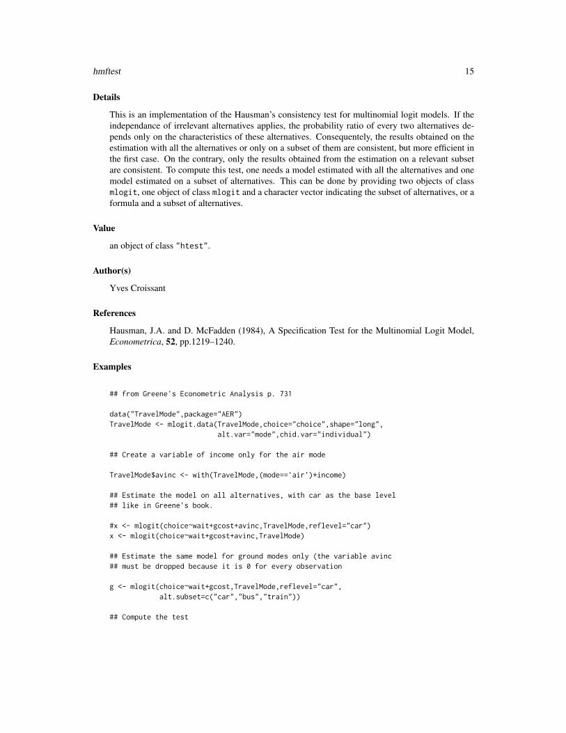
Details

This is an implementation of the Hausman’s consistency test for multinomial logit models. If theindependance of irrelevant alternatives applies, the probability ratio of every two alternatives de-pends only on the characteristics of these alternatives. Consequentely, the results obtained on theestimation with all the alternatives or only on a subset of them are consistent, but more efficient inthe first case. On the contrary, only the results obtained from the estimation on a relevant subsetare consistent. To compute this test, one needs a model estimated with all the alternatives and onemodel estimated on a subset of alternatives. This can be done by providing two objects of classmlogit, one object of class mlogit and a character vector indicating the subset of alternatives, or aformula and a subset of alternatives.

Value

an object of class "htest".

Author(s)

Yves Croissant

References

Hausman, J.A. and D. McFadden (1984), A Specification Test for the Multinomial Logit Model,Econometrica, 52, pp.1219–1240.

Examples

## from Greene's Econometric Analysis p. 731

data("TravelMode",package="AER")TravelMode <- mlogit.data(TravelMode,choice="choice",shape="long",

alt.var="mode",chid.var="individual")

## Create a variable of income only for the air mode

TravelMode$avinc <- with(TravelMode,(mode=='air')*income)

## Estimate the model on all alternatives, with car as the base level## like in Greene's book.

#x <- mlogit(choice~wait+gcost+avinc,TravelMode,reflevel="car")x <- mlogit(choice~wait+gcost+avinc,TravelMode)

## Estimate the same model for ground modes only (the variable avinc## must be dropped because it is 0 for every observation

g <- mlogit(choice~wait+gcost,TravelMode,reflevel="car",alt.subset=c("car","bus","train"))

## Compute the test

16 JapaneseFDI

hmftest(x,g)

JapaneseFDI Japanese Foreign Direct Investment in European Regions

Description

a cross-section


country : Europe

Usage

data(JapaneseFDI)

Format


firm the investment idcountry the countryregion the region (nuts1 nomenclature)choice a dummy indicating the chosen regionchoice.c the chosen countrywage wage rate in the regionunemp unemployment rate in the regionelig is the country eligible to european subsidiesarea the area of the regionscrate social charge rate (country level)ctaxrate corporate tax rate (country level)gdp regional gdpharris harris’ market potentialkrugman krugman’s market potentialdomind domestic industry countjapind japan industry countnetwork network count

Source

.

References

Head, Keith and Thierry Mayer (2004) “Market potential and the location of Japanese investmentin the european union”, the Review of Economics and Statistics, 86(4), 959-972.

Ketchup 17

Ketchup Choice of Brand for Ketchup

Description

a cross-section




Usage

data(Ketchup)

Format


hid individuals identifiers

id purchase identifiers

choice one of heinz, hunts, delmonte, stb (store brand)


Source

Kim, Byong–Do, Robert C. Blattberg and Peter E. Rossi (1995) “Modeling the distribution of pricesensitivity and implications for optimal retail pricing”, Journal of Business Economics and Statis-tics, 13(3), 291.

References


logsum Compute the log-sum or inclusive value/utility

Description

The logsum function computes the inclusive value, or inclusive utility, which is used to computethe surplus and to estimate the two steps nested logit model.



18 logsum

Usage

logsum(coef, X = NULL, formula = NULL, data = NULL,type = NULL, output = c("chid", "obs"))

Arguments

coef a numerical vector or a mlogit object, from which the coef vector is extracted,

X a matrix or a mlogit object from which the model.matrix is extracted,

formula a formula or a mlogit object from which the formula is extracted,

data a data.frame or a mlogit object from which the model.frame is extracted,

type either "group" or "global" : if a group argument has been provided in themlogit.data, the inclusive values are by default computed for every group,otherwise, a unique global inclusive value is computed for each choice situation,

output the shape of the results: if "chid", the results is a vector (if type = "global")or a matrix (if type = "region") with row number equal to the numberof choice situation, if "obs" a vector of length equal to the number of lines ofthe data in long format is returned.

Details

The inclusive value, or inclusive utility, or log-sum is the log of the denominator of the probabilitiesof the multinomial logit model. If a "group" variable is provided in the "mlogit.data" function,the denominator can either be the one of the multinomial model or those of the lower model of thenested logit model.

If only one argument (coef) is provided, it should a mlogit object and in this case, the coefficientsand the model.matrix are extracted from this model.

In order to provide a different model.matrix, further arguments could be used. X is a matrix or amlogit from which the model.matrix is extracted. The formula-data interface can also be usedto construct the relevant model.matrix.

Value

either a vector or a matrix.

Author(s)

Yves Croissant

See Also

mlogit for the estimation of a multinomial logit model.

mFormula 19

mFormula Model formula for logit models

Description

Two kinds of variables are used in logit models: alternative specific and individual specific variables.mFormula provides a relevant class to deal with this specificity and suitable methods to extract theelements of the model.

Usage

mFormula(object)## S3 method for class 'formula'mFormula(object)is.mFormula(object)## S3 method for class 'mFormula'model.matrix(object, data, ...)## S3 method for class 'mFormula'model.frame(formula, data, ..., lhs = NULL, rhs = NULL)

Arguments

object for the mFormula function, a formula, for the update and model.matrix meth-ods, a mFormula object,

formula a mFormula object,

data a data.frame,

lhs see Formula

rhs see Formula


Details

Let J being the number of alternatives. The formula may include alternative-specific and individualspecific variables. For the latter, J-1 coefficients are estimated for each variable. For the former,only one (generic) coefficient or J different coefficient may be estimated.

A mFormula is a formula for which the right hand side may contain three parts: the first one con-tains the alternative specific variables with generic coefficient, i.e. a unique coefficient for all thealternatives ; the second one contains the individual specific variables for which one coefficient isestimated for all the alternatives except one of them ; the third one contains the alternative specificvariables with alternative specific coefficients. The different parts are separeted by a “|” sign. Ifa standard formula is writen, it is assumed that there are only alternative specific variables withgeneric coefficients.

The intercept is necessarely alternative specific (a generic intercept is not identified because onlyutility differences are relevant). Therefore, it deals with the second part of the formula. As it isusual in R, the default behaviour is to include an intercept. A model without an intercept (which is

20 mlogit

hardly meaningfull) may be specified by includint +0 or -1 in the second rhs part of the formula. +0or -1 in the first and in the third part of the formula are simply ignored.

Specific methods are provided to build correctly the model matrix and to update the formula. ThemFormula function is not intended to be use directly. While using the mlogit function, the firstargument is automaticaly coerced to a mFormula object.

Value

an object of class mFormula.

Author(s)

Yves Croissant

Examples

data("Fishing", package = "mlogit")Fish <- mlogit.data(Fishing, varying = c(2:9), shape = "wide", choice ="mode")

# a formula with to alternative specific variables (price and catch) and# an interceptf1 <- mFormula(mode ~ price + catch)head(model.matrix(f1, Fish), 2)

# same, with an individual specific variable (income)f2 <- mFormula(mode ~ price + catch | income)head(model.matrix(f2, Fish), 2)

# same, without an interceptf3 <- mFormula(mode ~ price + catch | income + 0)head(model.matrix(f3, Fish), 2)

# same as f2, but now, coefficients of catch are alternative specificf4 <- mFormula(mode ~ price | income | catch)head(model.matrix(f4, Fish), 2)

mlogit Multinomial logit model

Description

Estimation by maximum likelihood of the multinomial logit model, with alternative-specific and/orindividual specific variables.

mlogit 21

Usage

mlogit(formula, data, subset, weights, na.action, start = NULL,alt.subset = NULL, reflevel = NULL,nests = NULL, un.nest.el = FALSE, unscaled = FALSE,heterosc = FALSE, rpar = NULL, probit = FALSE,R = 40, correlation = FALSE, halton = NULL,random.nb = NULL, panel = FALSE, estimate = TRUE,seed = 10, ...)

## S3 method for class 'mlogit'print(x, digits = max(3, getOption("digits") - 2),

width = getOption("width"), ...)## S3 method for class 'mlogit'summary(object, ...)## S3 method for class 'summary.mlogit'print(x, digits = max(3, getOption("digits") - 2),

width = getOption("width"), ...)## S3 method for class 'mlogit'print(x, digits = max(3, getOption("digits") - 2),

width = getOption("width"), ...)## S3 method for class 'mlogit'logLik(object, ...)## S3 method for class 'mlogit'residuals(object, outcome = TRUE, ...)## S3 method for class 'mlogit'fitted(object,

type = c("outcome", "probabilities","linpred", "parameters"),

outcome = NULL, ...)## S3 method for class 'mlogit'predict(object, newdata, returnData = FALSE, ...)## S3 method for class 'mlogit'df.residual(object, ...)## S3 method for class 'mlogit'terms(x, ...)## S3 method for class 'mlogit'model.matrix(object, ...)## S3 method for class 'mlogit'update(object, new, ...)## S3 method for class 'mlogit'coef(object, fixed = FALSE, ...)## S3 method for class 'summary.mlogit'coef(object, ...)

Arguments

x, object an object of class mlogit

formula a symbolic description of the model to be estimated,

new an updated formula for the update method,

22 mlogit

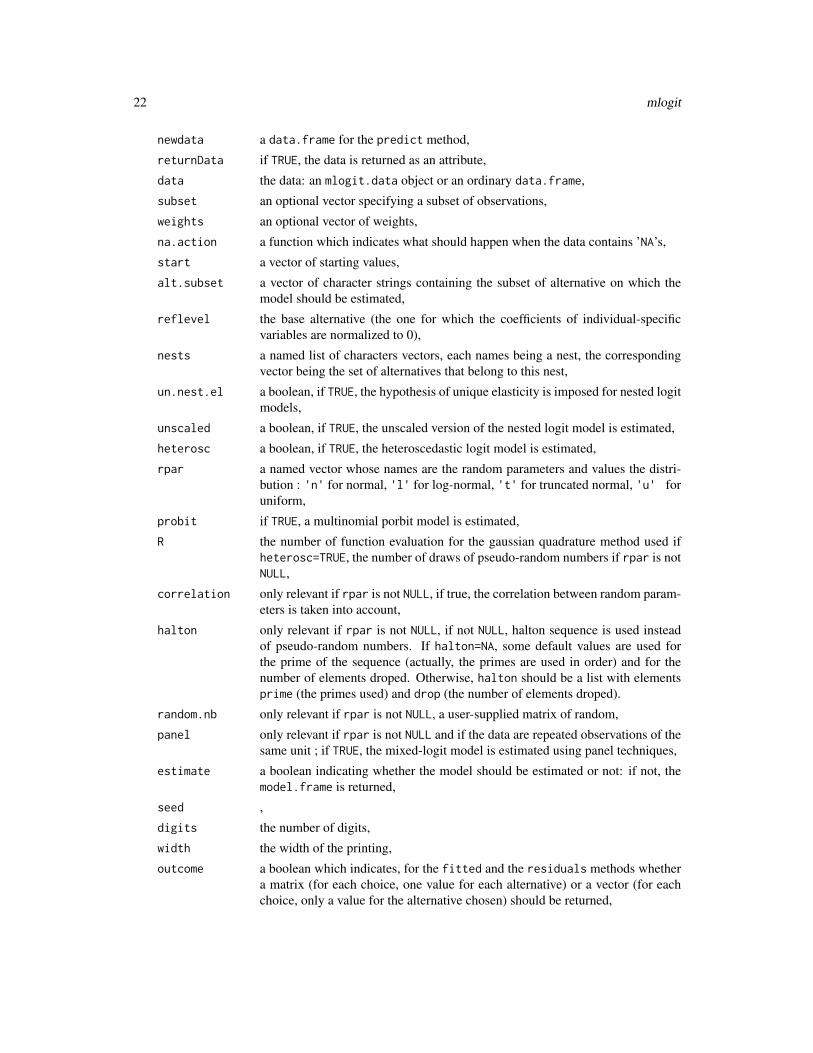
newdata a data.frame for the predict method,

returnData if TRUE, the data is returned as an attribute,

data the data: an mlogit.data object or an ordinary data.frame,

subset an optional vector specifying a subset of observations,

weights an optional vector of weights,

na.action a function which indicates what should happen when the data contains ’NA’s,

start a vector of starting values,

alt.subset a vector of character strings containing the subset of alternative on which themodel should be estimated,

reflevel the base alternative (the one for which the coefficients of individual-specificvariables are normalized to 0),

nests a named list of characters vectors, each names being a nest, the correspondingvector being the set of alternatives that belong to this nest,

un.nest.el a boolean, if TRUE, the hypothesis of unique elasticity is imposed for nested logitmodels,

unscaled a boolean, if TRUE, the unscaled version of the nested logit model is estimated,

heterosc a boolean, if TRUE, the heteroscedastic logit model is estimated,

rpar a named vector whose names are the random parameters and values the distri-bution : 'n' for normal, 'l' for log-normal, 't' for truncated normal, 'u' foruniform,

probit if TRUE, a multinomial porbit model is estimated,

R the number of function evaluation for the gaussian quadrature method used ifheterosc=TRUE, the number of draws of pseudo-random numbers if rpar is notNULL,

correlation only relevant if rpar is not NULL, if true, the correlation between random param-eters is taken into account,

halton only relevant if rpar is not NULL, if not NULL, halton sequence is used insteadof pseudo-random numbers. If halton=NA, some default values are used forthe prime of the sequence (actually, the primes are used in order) and for thenumber of elements droped. Otherwise, halton should be a list with elementsprime (the primes used) and drop (the number of elements droped).

random.nb only relevant if rpar is not NULL, a user-supplied matrix of random,

panel only relevant if rpar is not NULL and if the data are repeated observations of thesame unit ; if TRUE, the mixed-logit model is estimated using panel techniques,

estimate a boolean indicating whether the model should be estimated or not: if not, themodel.frame is returned,

seed ,

digits the number of digits,

width the width of the printing,

outcome a boolean which indicates, for the fitted and the residuals methods whethera matrix (for each choice, one value for each alternative) or a vector (for eachchoice, only a value for the alternative chosen) should be returned,

mlogit 23

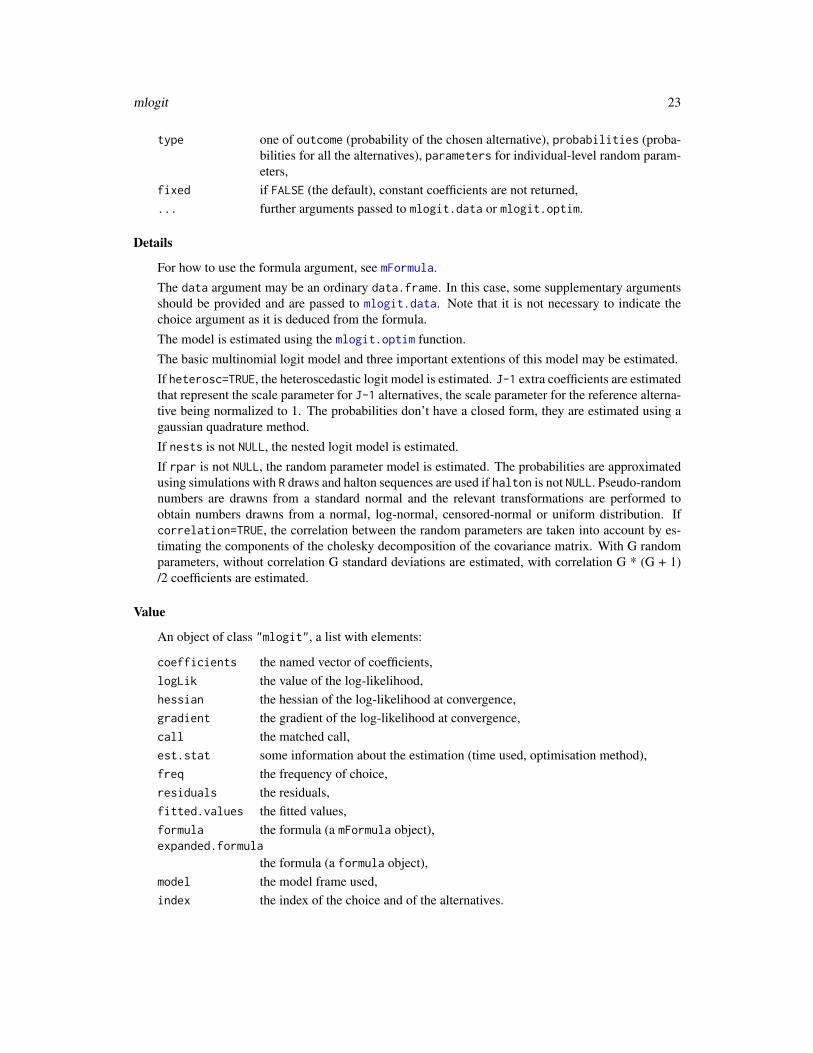
type one of outcome (probability of the chosen alternative), probabilities (proba-bilities for all the alternatives), parameters for individual-level random param-eters,

fixed if FALSE (the default), constant coefficients are not returned,... further arguments passed to mlogit.data or mlogit.optim.

Details

For how to use the formula argument, see mFormula.The data argument may be an ordinary data.frame. In this case, some supplementary argumentsshould be provided and are passed to mlogit.data. Note that it is not necessary to indicate thechoice argument as it is deduced from the formula.The model is estimated using the mlogit.optim function.The basic multinomial logit model and three important extentions of this model may be estimated.If heterosc=TRUE, the heteroscedastic logit model is estimated. J-1 extra coefficients are estimatedthat represent the scale parameter for J-1 alternatives, the scale parameter for the reference alterna-tive being normalized to 1. The probabilities don’t have a closed form, they are estimated using agaussian quadrature method.If nests is not NULL, the nested logit model is estimated.If rpar is not NULL, the random parameter model is estimated. The probabilities are approximatedusing simulations with R draws and halton sequences are used if halton is not NULL. Pseudo-randomnumbers are drawns from a standard normal and the relevant transformations are performed toobtain numbers drawns from a normal, log-normal, censored-normal or uniform distribution. Ifcorrelation=TRUE, the correlation between the random parameters are taken into account by es-timating the components of the cholesky decomposition of the covariance matrix. With G randomparameters, without correlation G standard deviations are estimated, with correlation G * (G + 1)/2 coefficients are estimated.

Value

An object of class "mlogit", a list with elements:

coefficients the named vector of coefficients,logLik the value of the log-likelihood,hessian the hessian of the log-likelihood at convergence,gradient the gradient of the log-likelihood at convergence,call the matched call,est.stat some information about the estimation (time used, optimisation method),freq the frequency of choice,residuals the residuals,fitted.values the fitted values,formula the formula (a mFormula object),expanded.formula

the formula (a formula object),model the model frame used,index the index of the choice and of the alternatives.

24 mlogit

Author(s)

Yves Croissant

References

McFadden, D. (1973) Conditional Logit Analysis of Qualitative Choice Behavior, in P. Zarembkaed., Frontiers in Econometrics, New-York: Academic Press.

McFadden, D. (1974) “The Measurement of Urban Travel Demand”, Journal of Public Economics,3, pp. 303-328.

Train, K. (2004) Discrete Choice Modelling, with Simulations, Cambridge University Press.

See Also

mlogit.data to shape the data. multinom from package nnet performs the estimation of themultinomial logit model with individual specific variables. mlogit.optim for details about theoptimization function.

Examples

## Cameron and Trivedi's Microeconometrics p.493 There are two## alternative specific variables : price and catch one individual## specific variable (income) and four fishing mode : beach, pier, boat,## charter

data("Fishing", package = "mlogit")Fish <- mlogit.data(Fishing, varying = c(2:9), shape = "wide", choice = "mode")

## a pure "conditional" model

summary(mlogit(mode ~ price + catch, data = Fish))

## a pure "multinomial model"

summary(mlogit(mode ~ 0 | income, data = Fish))

## which can also be estimated using multinom (package nnet)

library("nnet")summary(multinom(mode ~ income, data = Fishing))

## a "mixed" model

m <- mlogit(mode ~ price+ catch | income, data = Fish)summary(m)

## same model with charter as the reference level

m <- mlogit(mode ~ price+ catch | income, data = Fish, reflevel = "charter")

## same model with a subset of alternatives : charter, pier, beach

mlogit 25

m <- mlogit(mode ~ price+ catch | income, data = Fish,alt.subset = c("charter", "pier", "beach"))

## model on unbalanced data i.e. for some observations, some## alternatives are missing

# a data.frame in wide format with two missing pricesFishing2 <- FishingFishing2[1, "price.pier"] <- Fishing2[3, "price.beach"] <- NAmlogit(mode~price+catch|income, Fishing2, shape="wide", choice="mode", varying = 2:9)

# a data.frame in long format with three missing linesdata("TravelMode", package = "AER")Tr2 <- TravelMode[-c(2, 7, 9),]mlogit(choice~wait+gcost|income+size, Tr2, shape = "long",

chid.var = "individual", alt.var="mode", choice = "choice")

## An heteroscedastic logit model

data("TravelMode", package = "AER")hl <- mlogit(choice ~ wait + travel + vcost, TravelMode,

shape = "long", chid.var = "individual", alt.var = "mode",method = "bfgs", heterosc = TRUE, tol = 10)

## A nested logit model

TravelMode$avincome <- with(TravelMode, income * (mode == "air"))TravelMode$time <- with(TravelMode, travel + wait)/60TravelMode$timeair <- with(TravelMode, time * I(mode == "air"))TravelMode$income <- with(TravelMode, income / 10)

# Hensher and Greene (2002), table 1 p.8-9 model 5TravelMode$incomeother <- with(TravelMode, ifelse(mode %in% c('air', 'car'), income, 0))nl <- mlogit(choice~gcost+wait+incomeother, TravelMode,

shape='long', alt.var='mode',nests=list(public=c('train', 'bus'), other=c('car','air')))

# same with a comon nest elasticity (model 1)nl2 <- update(nl, un.nest.el = TRUE)

## a probit model## Not run:pr <- mlogit(choice ~ wait + travel + vcost, TravelMode,

shape = "long", chid.var = "individual", alt.var = "mode",probit = TRUE)

## End(Not run)

## a mixed logit model## Not run:rpl <- mlogit(mode ~ price+ catch | income, Fishing, varying = 2:9,

26 mlogit.data

shape = 'wide', rpar = c(price= 'n', catch = 'n'),correlation = TRUE, halton = NA,R = 10, tol = 10, print.level = 0)

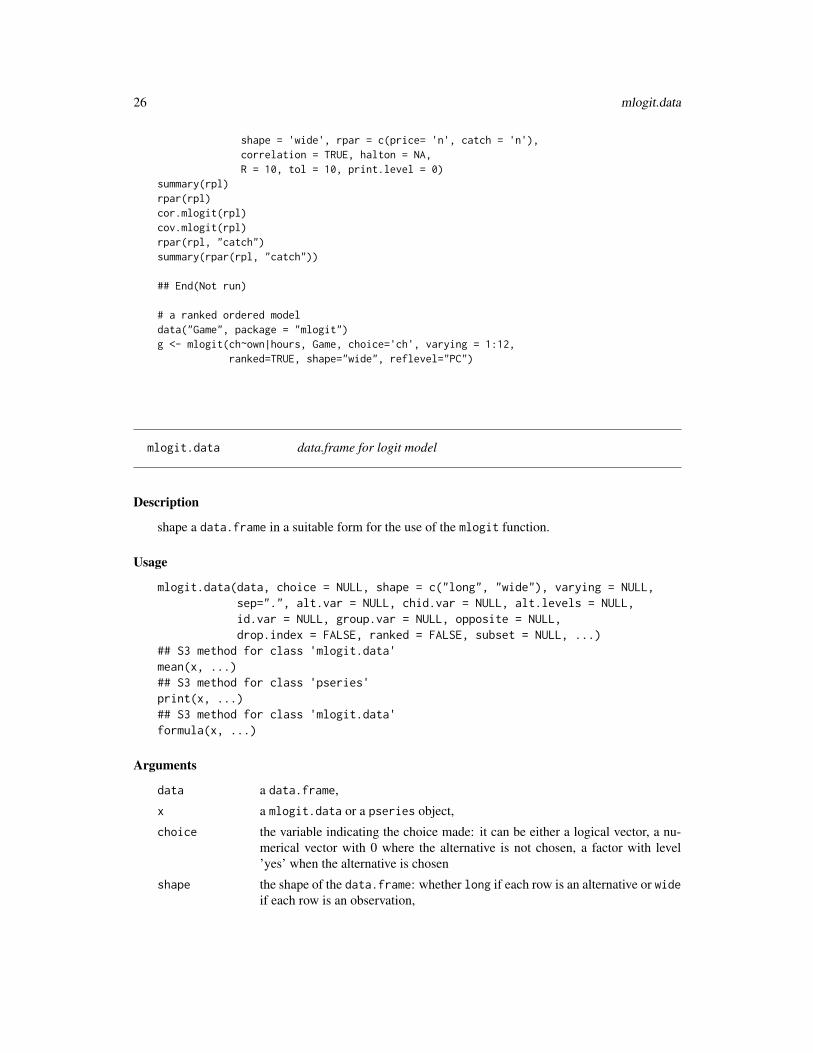
summary(rpl)rpar(rpl)cor.mlogit(rpl)cov.mlogit(rpl)rpar(rpl, "catch")summary(rpar(rpl, "catch"))

## End(Not run)

# a ranked ordered modeldata("Game", package = "mlogit")g <- mlogit(ch~own|hours, Game, choice='ch', varying = 1:12,

ranked=TRUE, shape="wide", reflevel="PC")

mlogit.data data.frame for logit model

Description

shape a data.frame in a suitable form for the use of the mlogit function.

Usage

mlogit.data(data, choice = NULL, shape = c("long", "wide"), varying = NULL,sep=".", alt.var = NULL, chid.var = NULL, alt.levels = NULL,id.var = NULL, group.var = NULL, opposite = NULL,drop.index = FALSE, ranked = FALSE, subset = NULL, ...)

## S3 method for class 'mlogit.data'mean(x, ...)## S3 method for class 'pseries'print(x, ...)## S3 method for class 'mlogit.data'formula(x, ...)

Arguments

data a data.frame,

x a mlogit.data or a pseries object,

choice the variable indicating the choice made: it can be either a logical vector, a nu-merical vector with 0 where the alternative is not chosen, a factor with level’yes’ when the alternative is chosen

shape the shape of the data.frame: whether long if each row is an alternative or wideif each row is an observation,

mlogit.data 27

varying the indexes of the variables that are alternative specific,

sep the seperator of the variable name and the alternative name (only relevant for awide data.frame),

alt.var the name of the variable that contains the alternative index (for a long data.frameonly) or the name under which the alternative index will be stored (the defaultname is alt),

chid.var the name of the variable that contains the choice index or the name under whichthe choice index will be stored,

alt.levels the name of the alternatives: if null, for a wide data.frame, they are guessedfrom the variable names and the choice variable (both should be the same), fora long data.frame, they are guessed from the alt.var argument,

id.var the name of the variable that contains the individual index if any,

group.var the name of the variable that contains the group index if any,

opposite returns the opposite of the specified variables,

drop.index should the index variables be dropped from the data.frame,

ranked a logical value which is true if the response is a rank,

subset a logical expression which defines the subset of observations to be selected,

... further arguments passed to reshape.

Value

A mlogit.data object, which is a data.frame in long format, i.e. one line for each alternative. Ithas a index attribute, which is a data.frame that contains the index of the choice made ('chid'),the index of the alternative ('alt') and, if any, the index of the individual ('id'). The choicevariable is a boolean which indicates the choice made. This function use reshape if the data.frameis in wide format.

Author(s)

Yves Croissant

See Also

reshape

Examples

# ModeChoice is a long data.frame

data("TravelMode", package = "AER")TM <- mlogit.data(TravelMode, choice = "choice", shape = "long",

alt.levels = c("air", "train", "bus", "car"))

# Same but the alt variable called mode is provided

TM <- mlogit.data(TravelMode ,choice = "choice", shape = "long",

28 mlogit.optim

alt.var = "mode")

# Same but the chid variable called individual is provided

TM <- mlogit.data(TravelMode, choice = "choice",shape = "long", id.var = "individual",alt.levels = c("air", "train", "bus", "car"))

# Same but with two own provided variables

TM <- mlogit.data(TravelMode, choice = "choice", shape = "long",id.var = "individual", alt.var = "mode")

# Same but with two own provided variables which are deleted from the# data.frame

TM <- mlogit.data(TravelMode, choice = "choice", shape = "long",id.var = "individual", alt.var = "mode", drop.index = TRUE)

# Train is a wide data.frame with columns 'choiceid' is the choice# index, the alternatives are named "ch1" and "ch2", the opposite of# the variables is returned

data("Train", package = "mlogit")Train <- mlogit.data(Train, choice = "choice", shape = "wide",

varying = 4:11, alt.levels = c("A", "B"), sep = "_",opposite = c("price", "time", "change", "comfort"))

# Car is a wide data.frame

data("Car", package = "mlogit")Car <- mlogit.data(Car, varying = 5:70, shape = "wide", sep = "",

choice = "choice", alt.levels = 1:6)

data("HC", package = "mlogit")HC <- mlogit.data(HC, choice = "depvar", varying=c(2:8, 10:16), shape="wide")

# Game is a data.frame in wide format for which the response is a# ranking variable

data("Game", package = "mlogit")G <- mlogit.data(Game, shape="wide", varying = 1:12, alt.var = 'platform',

drop.index = TRUE, choice="ch", ranked =TRUE)

# Game2 contains the same data, but in long formatdata("Game2", package = "mlogit")G2 <- mlogit.data(Game2, shape='long', choice="ch", alt.var = 'platform', ranked = TRUE)

mlogit.optim Non-linear minimization routine

mlogit.optim 29

Description

This function performs efficiently the optimization of the likelihood functions for multinomial logitmodels

Usage

mlogit.optim(logLik, start, method = c("bfgs", "nr", "bhhh"), iterlim = 2000,tol = 1E-06, ftol = 1e-08, steptol = 1e-10,print.level = 0, constPar = NULL, ...)

Arguments

logLik the likelihood function to be maximized,

start the initial value of the vector of coefficients,

method the method used, one of 'nr' for Newton-Ralphson, 'bhhh' for Berndt-Hausman-Hall-Hall and 'bfgs',

iterlim the maximum number of iterations,

tol the value of the criteria for the gradient,

ftol the value of the criteria for the function,

steptol the value of the criteria for the step,

print.level one of (0, 1, 2), the details of the printing messages. If 'print.level=0', noinformation about the optimization process is provided, if 'print.level=1' thevalue of the likelihood, the step and the stoping criteria is printing, if 'print.level=2'the vectors of the parameters and the gradient are also printed.

constPar a numeric or a character vector which indicates that some parameters should betreated as constant,

... further arguments passed to f.

Details

The optimization is performed by updating, at each iteration, the vector of parameters by the amountstep * direction, where step is a positive scalar and direction = H^-1 * g, where g is the gradientand H^-1 is an estimation of the inverse of the hessian. The choice of H^-1 depends on the methodchosen :

if method='nr', H is the hessian (i.e. is the second derivates matrix of the likelihood function),

if method = 'bhhh', H is the outer-product of the individual contributions of each individual to thegradient,

if method = 'bfgs', H^-1 is updated at each iteration using a formula that uses the variationsof the vector of parameters and the gradient. The initial value of the matrix is the inverse of theouter-product of the gradient (i.e. the bhh estimator of the hessian).

The initial step is 1 and, if the new value of the function is less than the previous value, it is dividedby two, until a higher value is obtained.

The routine stops when the gradient is sufficiently close to 0. The criteria is g * H^-1 * g which iscompared to the tol argument. It also may stops if the number of iterations equals iterlim.

30 MobilePhones

The function f has a initial.value argument which is the initial value of the likelihood. Thefunction is then evaluated a first time with a step equals to one. If the value is lower than the initialvalue, the step is divided by two until the likelihood increases. The gradient is then computed andthe function returns as attributes the gradient is the step. This method is more efficient than otherfunctions available for R :

For the optim and the maxLik functions, the function and the gradient should be provided as sepa-rate functions. But, for multinomial logit models, both depends on the probabilities which are themost time-consuming elements of the model to compute.

For the nlm function, the fonction returns the gradient as an attribute. The gradient is thereforecomputed at each iteration, even when the function is computed with a step that is unable to increasethe value of the likelihood.

Previous versions of mlogit depended on the 'maxLik' package. We kept the same interface,namely the start, method, iterlim, tol, print.level and constPar arguments.

The default method is 'bfgs', which is known to perform well, even if the likelihood function isnot well behaved and the default value for print.level=1, which means moderate printing.

A special default behavior is performed if a simple multinomial logit model is estimated. Indeed, forthis model, the likelihood function is concave, the analytical hessian is simple to write and the opti-mization is straightforward. Therefore, in this case, the default method is 'nr' and print.level=0.

Value

a list that contains the followings elements :

optimum the value of the function at the optimum, with attributes: gradi a matrix thatcontains the contribution of each individual to the gradient, gradient the gradi-ent and, if method='nr' hessian the hessian,

coefficients the vector of the parameters at the optimum,

est.stat a list that contains some information about the optimization : 'nb.iter' thenumber of iterations, 'eps' the value of the stoping criteria, 'method' themethod of optimization method used, 'message'

Author(s)

Yves Croissant

MobilePhones Stated Preferences survey for mobile phones

Description

a cross-section from 2003



country : Netherland

Mode 31

Usage

data(MobilePhones)

Format


alt the alternative, denoted by 1 or 2

choice 1 if the alternative is chosen, 0 otherwise

price purchase price in euros (100, 135 or 170)

mincost cost of a minute in euros (0.25, 0.30 or 0.35)

extras extra features of the telephone : a factor with levels games, internet (which means gamesand internet) and camera (which means games and internet and camera)

network a factor with levels KPNVodaphone and other

sms the cost of an sms in euros (0.17 or 0.23)

design a factor with levels basic or trendy

Source

Sandor Zsolt and Philip Hans Franses (2009) “Consumer price evaluations through choice experi-ments”, Journal of Applied Econometrics, 24, 517–535.

References


Mode Mode Choice

Description

a cross-section



Usage

data(Mode)

Format


choice one of car, carpool, bus or rail

cost.z cost of mode z

time.z time of mode z


32 ModeCanada

References


ModeCanada Mode Choice for the Montreal-Toronto Corridor

Description

a cross-section



Usage

data(ModeCanada)

Format


case the individual index

alt the alternative, one of train, car, bus and air,

choice one if the mode is chosen, zero otherwise,

cost monetary cost,

ivt in vehicule time,

ovt out vehicule time,

frequency frequency,

income income,

urban urban,

noalt the number of alternatives available.

References

Bhat, Chandra R. (1995) “A heteroscedastic extreme value model of intercity travel mode choice”,Transportation Research Part B, 29(6), 471-483.

Koppelman Franck S. and Chieh-Hua Wen (2001) “The paired combinatorial logit model:properties,estimation and application”, Transportation Research Part B, 75-89.

Wen, Chieh-Hua and Franck S. Koppelman (2001) “The generalized nested logit model”, Trans-portation Research Part B, 627-641.


NOx 33

Examples

data("ModeCanada", package = "mlogit")bususers <- with(ModeCanada, case[choice == 1 & alt == "bus"])ModeCanada <- subset(ModeCanada, ! case %in% bususers)ModeCanada <- subset(ModeCanada, noalt == 4)ModeCanada <- subset(ModeCanada, alt != "bus")ModeCanada$alt <- ModeCanada$alt[drop = TRUE]KoppWen00 <- mlogit.data(ModeCanada, shape='long', chid.var = 'case',

alt.var = 'alt', choice='choice',drop.index=TRUE)

pcl <- mlogit(choice~freq+cost+ivt+ovt, KoppWen00, reflevel='car',nests='pcl', constPar=c('iv.train.air'))

NOx Technologies to reduce NOx emissions

Description

a cross-section



economic topic : microeconomics

econometrics topic : discrete choice

Usage

data("NOx")

Format


chid the plant id,

34 plot.mlogit

alt the alternative,id the owner id,choice the chosen alternative,available a dummy indicating that the alternative is available,env the regulatory environment, one of 'regulated', 'deregulated' and 'public',post dummy for post-combustion polution control technology,cm dummy for combustion modification technology,lnb dummy for low NOx burners technology,age age of the plant (in deviation from the mean age).vcost variable cost,kcost capital cost,

Source

American Economic Association data archive : http://aeaweb.org/aer/.

References

Fowlie, Meredith (2010) “Emissions Trading, Electricity Restructuring, and Investment in PollutionAbatement”, American Economic Review, 100(3), 837-869.

plot.mlogit Plot of the distribution of estimated random parameters

Description

Methods for rpar and mlogit objects which provide a plot of the distribution of one or all of theestimated random parameters

Usage

## S3 method for class 'mlogit'plot(x, par = NULL, norm = NULL,

type = c("density", "probability"), ...)## S3 method for class 'rpar'plot(x, norm = NULL, type = c("density","probability"), ...)

Arguments

x a mlogit or a rpar object,type the function to be plotted, whether the density or the probability density func-

tion,par a subset of the random parameters ; if NULL, all the parameters are selected,norm the coefficient’s name for the mlogit method or the coefficient’s value for the

rpar method used for normalization,... further arguments, passed to plot.rpar for the mlogit method and to plot for

the rpar method.

http://aeaweb.org/aer/

RiskyTransport 35

Details

For the rpar method, one plot is drawn. For the mlogit method, one plot for each selected randomparameter is drawn.

Author(s)

Yves Croissant

See Also

mlogit for the estimation of random parameters logit models and rpar for the description of rparobjects and distribution for functions which return informations about the distribution of randomparameters.

RiskyTransport Risky Transportation Choices

Description

a cross-section


country : Sierra Leone

Usage

data(RiskyTransport)

Format


id individual id

choice 1 for the chosen mode

mode one of Helicopter, WaterTaxi, Ferry and Hovercraft

cost the generalised cost of the transport mode

risk the fatality rate, numbers of death per 100,000 trips

weight weights

seatsnoisecrowdnessconvlocclientelechid choice situation id

36 rpar

african yes if born in Africa, no otherwise

lifeExp declared life expectancy

dwage declared hourly wage

iwage imputed hourly wage

educ level of education, one of low and high

fatalism self-ranking of the degree of fatalism

gender gender, one of female and male

age age

haveChildren yes if the traveler has children, no otherwise

swim yes if the traveler knows how to swim, no itherwise

Source

American Economic Association data archive : http://aeaweb.org/aer/.

References

Gianmarco, Leon and Edward Miguel (2017) “Risky Transportation Choices and the Value of aStatistical Life”, American Economic Journal: Applied Economics, 9(1), 202-28.

rpar random parameter objects

Description

rpar objects contain the relevant information about estimated random parameters. The homony-mous function extract on rpar object from a mlogit object.

Usage

rpar(x, par = NULL, norm = NULL, ...)

Arguments

x a mlogit object,

par the name or the index of the parameters to be extracted ; if NULL, all the param-eters are selected,

norm the coefficient used for normalization if any,


Details

mlogit objects contain an element called rpar which contain a list of rpar objects, one for each es-timated random parameter. The print method prints the name of the distribution and the parameter,the summary behave like the one for numeric vectors.

http://aeaweb.org/aer/

scoretest 37

Value

a rpar object, which contain :

dist the name of the distribution,

mean the first parameter of the distribution,

sigma the second parameter of the distribution,

name the name of the parameter,

Author(s)

Yves Croissant

See Also

mlogit for the estimation of a random parameters logit model.

scoretest The three tests for mlogit models

Description

Three tests for mlogit models: specific methods for the Wald test and the likelihood ration test anda new function for the score test

Usage

scoretest(object, ...)## S3 method for class 'mlogit'scoretest(object, ...)## S3 method for class 'mlogit'waldtest(object, ...)## S3 method for class 'mlogit'lrtest(object, ...)

Arguments

object an object of class mlogit or a formula,

... two kinds of arguments can be used. If "mlogit" arguments are introduced,initial model is updated using these arguments. If "formula" or other "mlogit"models are introduced, the standard behavior of "waldtest" and "lrtest" isfollowed.

38 Telephone

Details

The "scoretest" function and "mlogit" method for "waldtest" and "lrtest" from the "lmtest"package provides the infrastructure to compute the three tests of hypothesis for "mlogit" objects.

The first argument must be a "mlogit" object. If the second one is a fitted model or a formula, thebehaviour of the three functions is the one of the default methods of "waldtest" and "lrtest":the two models provided should be nested and the hypothesis tested is that the constrained model isthe ‘right’ model.

If no second model is provided and if the model provided is the constrained model, some specificarguments of "mlogit" should be provided to descibe how the initial model should be updated. Ifthe first model is the unconstrained model, it is tested versus the ‘natural’ constrained model; forexample, if the model is a heteroscedastic logit model, the constrained one is the multinomial logitmodel.

Value

an object of class "htest".

Author(s)

Yves Croissant

Examples

library("mlogit")data("TravelMode", package = "AER")ml <- mlogit(choice ~ wait + travel + vcost, TravelMode,

shape = "long", chid.var = "individual", alt.var = "mode")hl <- mlogit(choice ~ wait + travel + vcost, TravelMode,

shape = "long", chid.var = "individual", alt.var = "mode",method = "bfgs", heterosc = TRUE)

lrtest(ml, hl)waldtest(hl)scoretest(ml, heterosc = TRUE)

Telephone Choice among residential telephone service options for local calling

Description




country : United-States

Usage

data(Train)

TollRoad 39

Format


choice a logical which indicates if the alternative has been chosen

service a telephone service option

household the household index

cost the logarithm of the cost

Source

Walker J.L., Ben-Akiva M. and D. Bolduc (2007) “Identification of parameters in normal errorcomponent logit-mixture (NECLM) models”, Journal of Applied Econometrics, 22, 1095–1125.

Train K.E., Mc Fadden D. and M. Ben-Akiva (1987) “The demand for local telephone service: afully discrete model of residential calling patterns and service choices”, Rand Journal of Economics,18(1), 109–123

References


TollRoad Stated Preferences survey for a toll road

Description

a panel from 1999-2000

number of observations : 1448 observations for 548 individuals


country : United-States

Usage

data(TollRoad)

Format


id the individual id

src the source of the data, one of br : revealed preference survey conducted by the BrookingsInstitution, bs : stated preferences survey conducted by the Brookings Institution and cal :revealed preferences survey conducted by the Californian Polytechnic State University

route the route chosen, one of express (the toll-road) or freeway (the free road)

toll.alt the monetary cost of the road (a for the free road)


40 Train

time.alt the median time of the trip on both highways for the given schedulereliability.alt the reliability of the trip length on both highways for the given schedule, measured

by the difference between the 80th and the 50th percentile of the trip lengthoccupance the number of people in the carsize the household sizesex one of male or femaleflexibility does the respondent declare having a flexible arrival time, a factor with levels yes or nodistance trip distance in milescommute a long-commute for trips longer than 45 minutes (a factor with levels yes or no)age3050 a factor with levels yes if the respondent is between 30 and 50 years old, no otherwiseincome a factor with levels low, medium and high

Source

Kenneth A. Small, Clifford Winston, Jia Yan (2005) “Uncovering the distribution of motorists’preferences for travel time and reliability”, Econometrica, 73(4), 1367-1382.

References

Econometrica data archive

Train Stated Preferences for Train Traveling

Description




country : Netherland

Usage

data(Train)

Format


id individual identifientchoiceid choice identifientchoice one of ’A’ or ’B’price\_z price of proposition z (z = ’A’, ’B’) in cents of guilderstime\_z travel time of proposition z (z = ’A’, ’B’) in minutescomfort\_z comfort of proposition z (z = ’A’, ’B’), 0, 1 or 2 in decreasing comfort orderchange\_z number of changes for proposition z (z = ’A’, ’B’)

Tuna 41

Source

Ben–Akiva, M., D. Bolduc and M. Bradley (1993) “Estimation of travel choice models with ran-domly distributed values of time”, Transportation Research Record, 1413, 88–97.

Meijer, Erik and Jan Rouwendal (2006) “Measuring welfare effects in models with random coeffi-cients”, Journal of Applied Econometrics, 21(2), 227-244.

References


Tuna Choice of Brand for Tuna

Description

a cross-section




Usage

data(Tuna)

Format


hid individuals identifiers

id purchase identifiers

choice one of skw (Starkist water), cosw (Chicken of the sea water), pw (store–specific privatelabel water), sko (Starkist oil), coso (Chicken of the sea oil)


Source

Kim, Byong–Do, Robert C. Blattberg and Peter E. Rossi (1995) “Modeling the distribution of pricesensitivity and implications for optimal retail pricing”, Journal of Business Economics and Statis-tics, 13(3), 291.

References





42 vcov.mlogit

vcov.mlogit vcov method for mlogit objects

Description

The vcov method for mlogit objects extract the covariance matrix of the coefficients, the errors orthe random parameters.

Usage

## S3 method for class 'mlogit'vcov(object, what = c('coefficient', 'errors', 'rpar'),

type = c('cov', 'cor', 'sd'), reflevel = NULL, ...)

Arguments

object a mlogit object,

what indicates which covariance matrix has to be extracted : the default value iscoefficients, in this case, vcov behaves as usual. If what equals errors thecovariance matrix of the errors of the model is returned. Finally, if what equalsrpar, the covariance matrix of the random parameters are extracted.

type with this argument, the covariance matrix may be returned (the default) ; thecorrelation matrix and the standard deviation vector may also be extracted.

reflevel relevent for the extraction of the errors of a multinomial probit model ; in thiscase the covariance matrix is of error differences is returned and, with this argu-ment, the alternative used for differentiation is indicated.


Details

This new interface replaces the cor.mlogit and cov.mlogit functions which are deprecated.

Author(s)

Yves Croissant

See Also

mlogit for the estimation of multinomial logit models.

Yogurt 43

Yogurt Choice of Brand for Yogurts

Description

a cross-section




Usage

data(Yogurt)

Format


id individuals identifiers

choice one of yoplait, dannon, hiland, weight (weight watcher)

feat.z is there a newspaper feature advertisement for brand z ?


Source


References




Index

∗Topic attributemlogit.data, 26

∗Topic datasetsBeef, 2Car, 3Catsup, 4Cracker, 6Electricity, 10Examples, 11Fishing, 11Game, 12HC, 13Heating, 13JapaneseFDI, 16Ketchup, 17MobilePhones, 30Mode, 31ModeCanada, 32NOx, 33RiskyTransport, 35Telephone, 38TollRoad, 39Train, 40Tuna, 41Yogurt, 43

∗Topic htesthmftest, 14scoretest, 37

∗Topic modelsmFormula, 19

∗Topic regressioncorrelation, 5distribution, 7effects.mlogit, 8logsum, 17mlogit, 20mlogit.optim, 29plot.mlogit, 34rpar, 36

vcov.mlogit, 42[[<-.mlogit.data (mlogit.data), 26$<-.mlogit.data (mlogit.data), 26

Beef, 2

Car, 3Catsup, 4coef.mlogit (mlogit), 20coef.summary.mlogit (mlogit), 20cor.mlogit (correlation), 5correlation, 5cov.mlogit (correlation), 5Cracker, 6

df.residual.mlogit (mlogit), 20distribution, 7, 35drpar (distribution), 7

effects.mlogit, 8Elec.mxl (Examples), 11Elec.mxl2 (Examples), 11Elec.mxl3 (Examples), 11Elec.mxl4 (Examples), 11Elec.mxl5 (Examples), 11Electricity, 10Examples, 11

Fish.mprobit (Examples), 11Fishing, 11fitted.mlogit (mlogit), 20formula.mlogit.data (mlogit.data), 26

Game, 12Game2 (Game), 12

HC, 13Heating, 13hmftest, 14

index (mlogit.data), 26

44

INDEX 45

is.mFormula (mFormula), 19

JapaneseFDI, 16

Ketchup, 17

logLik.mlogit (mlogit), 20logsum, 17lrtest (scoretest), 37

mean.mlogit (distribution), 7mean.mlogit.data (mlogit.data), 26mean.rpar (distribution), 7med (distribution), 7mFormula, 19, 23mlogit, 8, 9, 18, 20, 35, 37, 42mlogit.data, 23, 24, 26mlogit.optim, 23, 24, 28MobilePhones, 30Mode, 31ModeCanada, 32model.frame.mFormula (mFormula), 19model.matrix.mFormula (mFormula), 19model.matrix.mlogit (mlogit), 20multinom, 24

NOx, 33

p1 (Examples), 11p2 (Examples), 11plot.mlogit, 34plot.rpar (plot.mlogit), 34predict.mlogit (mlogit), 20print.mlogit (mlogit), 20print.pseries (mlogit.data), 26print.rpar (rpar), 36print.summary.mlogit (mlogit), 20prpar (distribution), 7

qrpar (distribution), 7

residuals.mlogit (mlogit), 20rg (distribution), 7RiskyTransport, 35rpar, 8, 35, 36

scoretest, 37stdev (distribution), 7suml (mlogit), 20summary.mlogit (mlogit), 20

summary.rpar (rpar), 36

Telephone, 38terms.mlogit (mlogit), 20TollRoad, 39Train, 40Train.ml (Examples), 11Train.mxlc (Examples), 11Train.mxlu (Examples), 11Tuna, 41

update.mlogit (mlogit), 20

vcov.mlogit, 42

waldtest (scoretest), 37

Yogurt, 43

package ‘mlogit’ - r · package ‘mlogit ’ april 20, 2018 ... correlation correlation...

Documents