package 'mlbench

Package ‘mlbench’February 20, 2015

Version 2.1-1

Title Machine Learning Benchmark Problems

Date 2010-12-10

Author Friedrich Leisch and Evgenia Dimitriadou.

Maintainer Friedrich Leisch <[email protected]>

Description A collection of artificial and real-world machine learningbenchmark problems, including, e.g., several data sets from theUCI repository.

Depends R (>= 2.10)

License GPL-2

Suggests lattice

ZipData No

Repository CRAN

Date/Publication 2012-07-10 11:51:32

NeedsCompilation yes

R topics documented:as.data.frame.mlbench . . . . . . . . . . . . . . . . . . . . . . . . . . . . . . . . . . . 2bayesclass . . . . . . . . . . . . . . . . . . . . . . . . . . . . . . . . . . . . . . . . . . 3BostonHousing . . . . . . . . . . . . . . . . . . . . . . . . . . . . . . . . . . . . . . . 3BreastCancer . . . . . . . . . . . . . . . . . . . . . . . . . . . . . . . . . . . . . . . . 6DNA . . . . . . . . . . . . . . . . . . . . . . . . . . . . . . . . . . . . . . . . . . . . . 7Glass . . . . . . . . . . . . . . . . . . . . . . . . . . . . . . . . . . . . . . . . . . . . 9HouseVotes84 . . . . . . . . . . . . . . . . . . . . . . . . . . . . . . . . . . . . . . . . 10Ionosphere . . . . . . . . . . . . . . . . . . . . . . . . . . . . . . . . . . . . . . . . . . 11LetterRecognition . . . . . . . . . . . . . . . . . . . . . . . . . . . . . . . . . . . . . . 13mlbench.2dnormals . . . . . . . . . . . . . . . . . . . . . . . . . . . . . . . . . . . . . 14mlbench.cassini . . . . . . . . . . . . . . . . . . . . . . . . . . . . . . . . . . . . . . . 15mlbench.circle . . . . . . . . . . . . . . . . . . . . . . . . . . . . . . . . . . . . . . . . 16mlbench.cuboids . . . . . . . . . . . . . . . . . . . . . . . . . . . . . . . . . . . . . . 16mlbench.friedman1 . . . . . . . . . . . . . . . . . . . . . . . . . . . . . . . . . . . . . 17

1

2 as.data.frame.mlbench

mlbench.friedman2 . . . . . . . . . . . . . . . . . . . . . . . . . . . . . . . . . . . . . 18mlbench.friedman3 . . . . . . . . . . . . . . . . . . . . . . . . . . . . . . . . . . . . . 19mlbench.hypercube . . . . . . . . . . . . . . . . . . . . . . . . . . . . . . . . . . . . . 20mlbench.peak . . . . . . . . . . . . . . . . . . . . . . . . . . . . . . . . . . . . . . . . 20mlbench.ringnorm . . . . . . . . . . . . . . . . . . . . . . . . . . . . . . . . . . . . . . 21mlbench.shapes . . . . . . . . . . . . . . . . . . . . . . . . . . . . . . . . . . . . . . . 22mlbench.simplex . . . . . . . . . . . . . . . . . . . . . . . . . . . . . . . . . . . . . . 22mlbench.smiley . . . . . . . . . . . . . . . . . . . . . . . . . . . . . . . . . . . . . . . 23mlbench.spirals . . . . . . . . . . . . . . . . . . . . . . . . . . . . . . . . . . . . . . . 24mlbench.threenorm . . . . . . . . . . . . . . . . . . . . . . . . . . . . . . . . . . . . . 24mlbench.twonorm . . . . . . . . . . . . . . . . . . . . . . . . . . . . . . . . . . . . . . 25mlbench.waveform . . . . . . . . . . . . . . . . . . . . . . . . . . . . . . . . . . . . . 26mlbench.xor . . . . . . . . . . . . . . . . . . . . . . . . . . . . . . . . . . . . . . . . . 27Ozone . . . . . . . . . . . . . . . . . . . . . . . . . . . . . . . . . . . . . . . . . . . . 28PimaIndiansDiabetes . . . . . . . . . . . . . . . . . . . . . . . . . . . . . . . . . . . . 29plot.mlbench . . . . . . . . . . . . . . . . . . . . . . . . . . . . . . . . . . . . . . . . 30Satellite . . . . . . . . . . . . . . . . . . . . . . . . . . . . . . . . . . . . . . . . . . . 31Servo . . . . . . . . . . . . . . . . . . . . . . . . . . . . . . . . . . . . . . . . . . . . 33Shuttle . . . . . . . . . . . . . . . . . . . . . . . . . . . . . . . . . . . . . . . . . . . . 34Sonar . . . . . . . . . . . . . . . . . . . . . . . . . . . . . . . . . . . . . . . . . . . . 35Soybean . . . . . . . . . . . . . . . . . . . . . . . . . . . . . . . . . . . . . . . . . . . 36Vehicle . . . . . . . . . . . . . . . . . . . . . . . . . . . . . . . . . . . . . . . . . . . 38Vowel . . . . . . . . . . . . . . . . . . . . . . . . . . . . . . . . . . . . . . . . . . . . 39Zoo . . . . . . . . . . . . . . . . . . . . . . . . . . . . . . . . . . . . . . . . . . . . . 40

Index 42

as.data.frame.mlbench Convert an mlbench object to a dataframe

Description

Converts x (which is basically a list) to a dataframe.

Usage

## S3 method for class 'mlbench'as.data.frame(x, row.names=NULL, optional=FALSE, ...)

Arguments

x Object of class "mlbench".row.names,optional,...

currently ignored.

bayesclass 3

Examples

p <- mlbench.xor(5)pas.data.frame(p)

bayesclass Bayes classifier

Description

Returns the decision of the (optimal) Bayes classifier for a given data set. This is a generic function,i.e., there are different methods for the various mlbench problems.

If the classes of the problem do not overlap, then the Bayes decision is identical to the true classi-fication, which is implemented as the dummy function bayesclass.noerr (which simply returnsz$classes and is used for all problems with disjunct classes).

Usage

bayesclass(z)

Arguments

z An object of class "mlbench".

Examples

# 6 overlapping classesp <- mlbench.2dnormals(500,6)plot(p)

plot(p$x, col=as.numeric(bayesclass(p)))

BostonHousing Boston Housing Data

Description

Housing data for 506 census tracts of Boston from the 1970 census. The dataframe BostonHousingcontains the original data by Harrison and Rubinfeld (1979), the dataframe BostonHousing2 thecorrected version with additional spatial information (see references below).

Usage

data(BostonHousing)data(BostonHousing2)

4 BostonHousing

Format

The original data are 506 observations on 14 variables, medv being the target variable:

BostonHousing 5

crim per capita crime rate by townzn proportion of residential land zoned for lots over 25,000 sq.ftindus proportion of non-retail business acres per townchas Charles River dummy variable (= 1 if tract bounds river; 0 otherwise)nox nitric oxides concentration (parts per 10 million)rm average number of rooms per dwellingage proportion of owner-occupied units built prior to 1940dis weighted distances to five Boston employment centresrad index of accessibility to radial highwaystax full-value property-tax rate per USD 10,000ptratio pupil-teacher ratio by townb 1000(B − 0.63)2 where B is the proportion of blacks by townlstat percentage of lower status of the populationmedv median value of owner-occupied homes in USD 1000’s

The corrected data set has the following additional columns:

cmedv corrected median value of owner-occupied homes in USD 1000’stown name of towntract census tractlon longitude of census tractlat latitude of census tract

Source

The original data have been taken from the UCI Repository Of Machine Learning Databases at

• http://www.ics.uci.edu/~mlearn/MLRepository.html,

the corrected data have been taken from Statlib at

• http://lib.stat.cmu.edu/datasets/

See Statlib and references there for details on the corrections. Both were converted to R format byFriedrich Leisch.

References

Harrison, D. and Rubinfeld, D.L. (1978). Hedonic prices and the demand for clean air. Journal ofEnvironmental Economics and Management, 5, 81–102.

Gilley, O.W., and R. Kelley Pace (1996). On the Harrison and Rubinfeld Data. Journal of Environ-mental Economics and Management, 31, 403–405. [Provided corrections and examined censoring.]

Newman, D.J. & Hettich, S. & Blake, C.L. & Merz, C.J. (1998). UCI Repository of machinelearning databases [http://www.ics.uci.edu/~mlearn/MLRepository.html]. Irvine, CA: Universityof California, Department of Information and Computer Science.

Pace, R. Kelley, and O.W. Gilley (1997). Using the Spatial Configuration of the Data to Improve Es-timation. Journal of the Real Estate Finance and Economics, 14, 333–340. [Added georeferencingand spatial estimation.]

http://www.ics.uci.edu/~mlearn/MLRepository.html

http://lib.stat.cmu.edu/datasets/

6 BreastCancer

Examples

data(BostonHousing)summary(BostonHousing)

data(BostonHousing2)summary(BostonHousing2)

BreastCancer Wisconsin Breast Cancer Database

Description

The objective is to identify each of a number of benign or malignant classes. Samples arrive peri-odically as Dr. Wolberg reports his clinical cases. The database therefore reflects this chronologicalgrouping of the data. This grouping information appears immediately below, having been removedfrom the data itself. Each variable except for the first was converted into 11 primitive numericalattributes with values ranging from 0 through 10. There are 16 missing attribute values. See citedbelow for more details.

Usage

data(BreastCancer)

Format

A data frame with 699 observations on 11 variables, one being a character variable, 9 being orderedor nominal, and 1 target class.

[,1] Id Sample code number[,2] Cl.thickness Clump Thickness[,3] Cell.size Uniformity of Cell Size[,4] Cell.shape Uniformity of Cell Shape[,5] Marg.adhesion Marginal Adhesion[,6] Epith.c.size Single Epithelial Cell Size[,7] Bare.nuclei Bare Nuclei[,8] Bl.cromatin Bland Chromatin[,9] Normal.nucleoli Normal Nucleoli[,10] Mitoses Mitoses[,11] Class Class

Source

• Creator: Dr. WIlliam H. Wolberg (physician); University of Wisconsin Hospital ;Madison;Wisconsin; USA

• Donor: Olvi Mangasarian ([email protected])• Received: David W. Aha ([email protected])

These data have been taken from the UCI Repository Of Machine Learning Databases at

DNA 7

• ftp://ftp.ics.uci.edu/pub/machine-learning-databases

• http://www.ics.uci.edu/~mlearn/MLRepository.html

and were converted to R format by Evgenia Dimitriadou.

References

1. Wolberg,W.H., \& Mangasarian,O.L. (1990). Multisurface method of pattern separation formedical diagnosis applied to breast cytology. In Proceedings of the National Academy of Sciences,87, 9193-9196.- Size of data set: only 369 instances (at that point in time)- Collected classification results: 1 trial only- Two pairs of parallel hyperplanes were found to be consistent with 50% of the data- Accuracy on remaining 50% of dataset: 93.5%- Three pairs of parallel hyperplanes were found to be consistent with 67% of data- Accuracy on remaining 33% of dataset: 95.9%

2. Zhang,J. (1992). Selecting typical instances in instance-based learning. In Proceedings of theNinth International Machine Learning Conference (pp. 470-479). Aberdeen, Scotland: MorganKaufmann.- Size of data set: only 369 instances (at that point in time)- Applied 4 instance-based learning algorithms- Collected classification results averaged over 10 trials- Best accuracy result:- 1-nearest neighbor: 93.7%- trained on 200 instances, tested on the other 169- Also of interest:- Using only typical instances: 92.2% (storing only 23.1 instances)- trained on 200 instances, tested on the other 169


Examples

data(BreastCancer)summary(BreastCancer)

DNA Primate splice-junction gene sequences (DNA)

Description

It consists of 3,186 data points (splice junctions). The data points are described by 180 indicatorbinary variables and the problem is to recognize the 3 classes (ei, ie, neither), i.e., the boundariesbetween exons (the parts of the DNA sequence retained after splicing) and introns (the parts of theDNA sequence that are spliced out).

ftp://ftp.ics.uci.edu/pub/machine-learning-databases


8 DNA

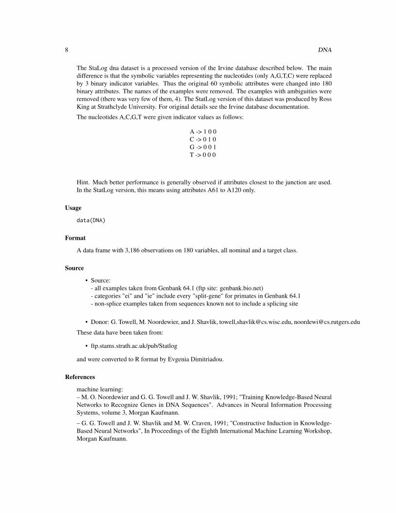
The StaLog dna dataset is a processed version of the Irvine database described below. The maindifference is that the symbolic variables representing the nucleotides (only A,G,T,C) were replacedby 3 binary indicator variables. Thus the original 60 symbolic attributes were changed into 180binary attributes. The names of the examples were removed. The examples with ambiguities wereremoved (there was very few of them, 4). The StatLog version of this dataset was produced by RossKing at Strathclyde University. For original details see the Irvine database documentation.

The nucleotides A,C,G,T were given indicator values as follows:

A -> 1 0 0C -> 0 1 0G -> 0 0 1T -> 0 0 0

Hint. Much better performance is generally observed if attributes closest to the junction are used.In the StatLog version, this means using attributes A61 to A120 only.

Usage

data(DNA)

Format

A data frame with 3,186 observations on 180 variables, all nominal and a target class.

Source

• Source:- all examples taken from Genbank 64.1 (ftp site: genbank.bio.net)- categories "ei" and "ie" include every "split-gene" for primates in Genbank 64.1- non-splice examples taken from sequences known not to include a splicing site

• Donor: G. Towell, M. Noordewier, and J. Shavlik, towell,[email protected], [email protected]

These data have been taken from:

• ftp.stams.strath.ac.uk/pub/Statlog


References

machine learning:– M. O. Noordewier and G. G. Towell and J. W. Shavlik, 1991; "Training Knowledge-Based NeuralNetworks to Recognize Genes in DNA Sequences". Advances in Neural Information ProcessingSystems, volume 3, Morgan Kaufmann.

– G. G. Towell and J. W. Shavlik and M. W. Craven, 1991; "Constructive Induction in Knowledge-Based Neural Networks", In Proceedings of the Eighth International Machine Learning Workshop,Morgan Kaufmann.

Glass 9

– G. G. Towell, 1991; "Symbolic Knowledge and Neural Networks: Insertion, Refinement, andExtraction", PhD Thesis, University of Wisconsin - Madison.

– G. G. Towell and J. W. Shavlik, 1992; "Interpretation of Artificial Neural Networks: MappingKnowledge-based Neural Networks into Rules", In Advances in Neural Information ProcessingSystems, volume 4, Morgan Kaufmann.

Examples

data(DNA)summary(DNA)

Glass Glass Identification Database

Description

A data frame with 214 observation containing examples of the chemical analysis of 7 different typesof glass. The problem is to forecast the type of class on basis of the chemical analysis. The studyof classification of types of glass was motivated by criminological investigation. At the scene of thecrime, the glass left can be used as evidence (if it is correctly identified!).

Usage

data(Glass)

Format

A data frame with 214 observations on 10 variables:

[,1] RI refractive index[,2] Na Sodium[,3] Mg Magnesium[,4] Al Aluminum[,5] Si Silicon[,6] K Potassium[,7] Ca Calcium[,8] Ba Barium[,9] Fe Iron

[,10] Type Type of glass (class attribute)

Source

• Creator: B. German, Central Research Establishment, Home Office Forensic Science Service,Aldermaston, Reading, Berkshire RG7 4PN

• Donor: Vina Spiehler, Ph.D., DABFT, Diagnostic Products Corporation


10 HouseVotes84



and were converted to R format by Friedrich Leisch.

References


Examples

data(Glass)summary(Glass)

HouseVotes84 United States Congressional Voting Records 1984

Description

This data set includes votes for each of the U.S. House of Representatives Congressmen on the 16key votes identified by the CQA. The CQA lists nine different types of votes: voted for, pairedfor, and announced for (these three simplified to yea), voted against, paired against, and announcedagainst (these three simplified to nay), voted present, voted present to avoid conflict of interest, anddid not vote or otherwise make a position known (these three simplified to an unknown disposition).

Usage

data(HouseVotes84)

Format

A data frame with 435 observations on 17 variables:

1 Class Name: 2 (democrat, republican)2 handicapped-infants: 2 (y,n)3 water-project-cost-sharing: 2 (y,n)4 adoption-of-the-budget-resolution: 2 (y,n)5 physician-fee-freeze: 2 (y,n)6 el-salvador-aid: 2 (y,n)7 religious-groups-in-schools: 2 (y,n)8 anti-satellite-test-ban: 2 (y,n)9 aid-to-nicaraguan-contras: 2 (y,n)

10 mx-missile: 2 (y,n)11 immigration: 2 (y,n)12 synfuels-corporation-cutback: 2 (y,n)13 education-spending: 2 (y,n)



Ionosphere 11

14 superfund-right-to-sue: 2 (y,n)15 crime: 2 (y,n)16 duty-free-exports: 2 (y,n)17 export-administration-act-south-africa: 2 (y,n)

Source

• Source: Congressional Quarterly Almanac, 98th Congress, 2nd session 1984, Volume XL:Congressional Quarterly Inc., ington, D.C., 1985

• Donor: Jeff Schlimmer ([email protected])





References


Examples

data(HouseVotes84)summary(HouseVotes84)

Ionosphere Johns Hopkins University Ionosphere database

Description

This radar data was collected by a system in Goose Bay, Labrador. This system consists of a phasedarray of 16 high-frequency antennas with a total transmitted power on the order of 6.4 kilowatts.See the paper for more details. The targets were free electrons in the ionosphere. "good" radarreturns are those showing evidence of some type of structure in the ionosphere. "bad" returns arethose that do not; their signals pass through the ionosphere.

Received signals were processed using an autocorrelation function whose arguments are the time ofa pulse and the pulse number. There were 17 pulse numbers for the Goose Bay system. Instancesin this databse are described by 2 attributes per pulse number, corresponding to the complex valuesreturned by the function resulting from the complex electromagnetic signal. See cited below formore details.

Usage

data(Ionosphere)



12 Ionosphere

Format

A data frame with 351 observations on 35 independent variables, some numerical and 2 nominal,and one last defining the class.

Source

• Source: Space Physics Group; Applied Physics Laboratory; Johns Hopkins University; JohnsHopkins Road; Laurel; MD 20723

• Donor: Vince Sigillito ([email protected])





References

Sigillito, V. G., Wing, S. P., Hutton, L. V., \& Baker, K. B. (1989). Classification of radar returnsfrom the ionosphere using neural networks. Johns Hopkins APL Technical Digest, 10, 262-266.

They investigated using backprop and the perceptron training algorithm on this database. Using thefirst 200 instances for training, which were carefully split almost 50% positive and 50% negative,they found that a "linear" perceptron attained 90.7%, a "non-linear" perceptron attained 92%, andbackprop an average of over 96% accuracy on the remaining 150 test instances, consisting of 123"good" and only 24 "bad" instances. (There was a counting error or some mistake somewhere;there are a total of 351 rather than 350 instances in this domain.) Accuracy on "good" instanceswas much higher than for "bad" instances. Backprop was tested with several different numbers ofhidden units (in [0,15]) and incremental results were also reported (corresponding to how well thedifferent variants of backprop did after a periodic number of epochs).

David Aha ([email protected]) briefly investigated this database. He found that nearest neighborattains an accuracy of 92.1%, that Ross Quinlan’s C4 algorithm attains 94.0% (no windowing),and that IB3 (Aha \& Kibler, IJCAI-1989) attained 96.7% (parameter settings: 70% and 80% foracceptance and dropping respectively).


Examples

data(Ionosphere)summary(Ionosphere)



LetterRecognition 13

LetterRecognition Letter Image Recognition Data

Description

The objective is to identify each of a large number of black-and-white rectangular pixel displays asone of the 26 capital letters in the English alphabet. The character images were based on 20 differentfonts and each letter within these 20 fonts was randomly distorted to produce a file of 20,000 uniquestimuli. Each stimulus was converted into 16 primitive numerical attributes (statistical moments andedge counts) which were then scaled to fit into a range of integer values from 0 through 15. Wetypically train on the first 16000 items and then use the resulting model to predict the letter categoryfor the remaining 4000. See the article cited below for more details.

Usage

data(LetterRecognition)

Format

A data frame with 20,000 observations on 17 variables, the first is a factor with levels A-Z, theremaining 16 are numeric.

[,1] lettr capital letter[,2] x.box horizontal position of box[,3] y.box vertical position of box[,4] width width of box[,5] high height of box[,6] onpix total number of on pixels[,7] x.bar mean x of on pixels in box[,8] y.bar mean y of on pixels in box[,9] x2bar mean x variance

[,10] y2bar mean y variance[,11] xybar mean x y correlation[,12] x2ybr mean of x2y[,13] xy2br mean of xy2

[,14] x.ege mean edge count left to right[,15] xegvy correlation of x.ege with y[,16] y.ege mean edge count bottom to top[,17] yegvx correlation of y.ege with x

Source

• Creator: David J. Slate

• Odesta Corporation; 1890 Maple Ave; Suite 115; Evanston, IL 60201

• Donor: David J. Slate ([email protected]) (708) 491-3867

14 mlbench.2dnormals





References

P. W. Frey and D. J. Slate (Machine Learning Vol 6/2 March 91): "Letter Recognition UsingHolland-style Adaptive Classifiers".

The research for this article investigated the ability of several variations of Holland-style adaptiveclassifier systems to learn to correctly guess the letter categories associated with vectors of 16integer attributes extracted from raster scan images of the letters. The best accuracy obtained was alittle over 80%. It would be interesting to see how well other methods do with the same data.


Examples

data(LetterRecognition)summary(LetterRecognition)

mlbench.2dnormals 2-dimensional Gaussian Problem

Description

Each of the cl classes consists of a 2-dimensional Gaussian. The centers are equally spaced on acircle around the origin with radius r.

Usage

mlbench.2dnormals(n, cl=2, r=sqrt(cl), sd=1)

Arguments

n number of patterns to createcl number of classesr radius at which the centers of the classes are locatedsd standard deviation of the Gaussians

Value

Returns an object of class "bayes.2dnormals" with components

x input valuesclasses factor vector of length n with target classes



mlbench.cassini 15

Examples

# 2 classesp <- mlbench.2dnormals(500,2)plot(p)# 6 classesp <- mlbench.2dnormals(500,6)plot(p)

mlbench.cassini Cassini: A 2 Dimensional Problem

Description

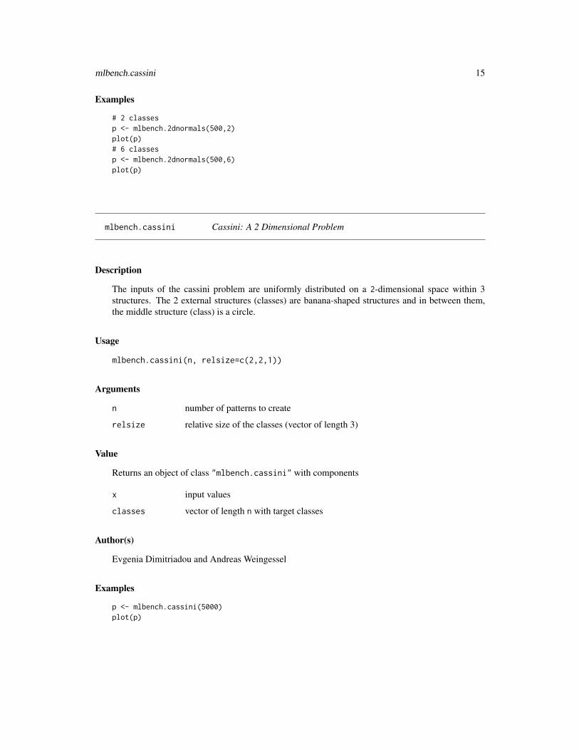
The inputs of the cassini problem are uniformly distributed on a 2-dimensional space within 3structures. The 2 external structures (classes) are banana-shaped structures and in between them,the middle structure (class) is a circle.

Usage

mlbench.cassini(n, relsize=c(2,2,1))

Arguments

n number of patterns to create

relsize relative size of the classes (vector of length 3)

Value

Returns an object of class "mlbench.cassini" with components

x input values

classes vector of length n with target classes

Author(s)

Evgenia Dimitriadou and Andreas Weingessel

Examples

p <- mlbench.cassini(5000)plot(p)

16 mlbench.cuboids

mlbench.circle Circle in a Square Problem

Description

The inputs of the circle problem are uniformly distributed on the d-dimensional cube with corners{±1}. This is a 2-class problem: The first class is a d-dimensional ball in the middle of the cube,the remainder forms the second class. The size of the ball is chosen such that both classes haveequal prior probability 0.5.

Usage

mlbench.circle(n, d=2)

Arguments


d dimension of the circle problem

Value

Returns an object of class "mlbench.circle" with components

x input values

classes factor vector of length n with target classes

Examples

# 2d examplep<-mlbench.circle(300,2)plot(p)## 3d examplep<-mlbench.circle(300,3)plot(p)

mlbench.cuboids Cuboids: A 3 Dimensional Problem

Description

The inputs of the cuboids problem are uniformly distributed on a 3-dimensional space within 3cuboids and a small cube in the middle of them.

Usage

mlbench.cuboids(n, relsize=c(2,2,2,1))

mlbench.friedman1 17

Arguments


relsize relative size of the classes (vector of length 4)

Value

Returns an object of class "mlbench.cuboids" with components

x input values

classes vector of length n with target classes

Author(s)

Evgenia Dimitriadou, and Andreas Weingessel

Examples

p <- mlbench.cuboids(7000)plot(p)## Not run:library(Rggobi)g <- ggobi(p$x)g$setColors(p$class)g$setMode("2D Tour")

## End(Not run)

mlbench.friedman1 Benchmark Problem Friedman 1

Description

The regression problem Friedman 1 as described in Friedman (1991) and Breiman (1996). Inputsare 10 independent variables uniformly distributed on the interval [0, 1], only 5 out of these 10 areactually used. Outputs are created according to the formula

y = 10 sin(πx1x2) + 20(x3− 0.5)2 + 10x4 + 5x5 + e

where e is N(0,sd).

Usage

mlbench.friedman1(n, sd=1)

Arguments


sd Standard deviation of noise

18 mlbench.friedman2

Value

Returns a list with components

x input values (independent variables)y output values (dependent variable)

References

Breiman, Leo (1996) Bagging predictors. Machine Learning 24, pages 123-140.

Friedman, Jerome H. (1991) Multivariate adaptive regression splines. The Annals of Statistics 19(1), pages 1-67.


Description

The regression problem Friedman 2 as described in Friedman (1991) and Breiman (1996). Inputsare 4 independent variables uniformly distrtibuted over the ranges

0 ≤ x1 ≤ 100

40π ≤ x2 ≤ 560π

0 ≤ x3 ≤ 1

1 ≤ x4 ≤ 11

The outputs are created according to the formula

y = (x12 + (x2x3− (1/(x2x4)))2)0.5 + e

where e is N(0,sd).

Usage

mlbench.friedman2(n, sd=125)

Arguments

n number of patterns to createsd Standard deviation of noise. The default value of 125 gives a signal to noise

ratio (i.e., the ratio of the standard deviations) of 3:1. Thus, the variance of thefunction itself (without noise) accounts for 90% of the total variance.

Value



mlbench.friedman3 19

References




Description

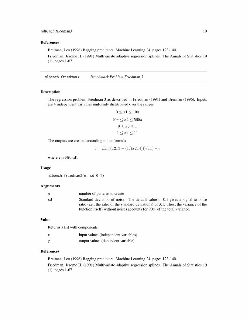
The regression problem Friedman 3 as described in Friedman (1991) and Breiman (1996). Inputsare 4 independent variables uniformly distrtibuted over the ranges

0 ≤ x1 ≤ 100

40π ≤ x2 ≤ 560π

0 ≤ x3 ≤ 1

1 ≤ x4 ≤ 11

The outputs are created according to the formula

y = atan((x2x3− (1/(x2x4)))/x1) + e

where e is N(0,sd).

Usage

mlbench.friedman3(n, sd=0.1)

Arguments

n number of patterns to createsd Standard deviation of noise. The default value of 0.1 gives a signal to noise

ratio (i.e., the ratio of the standard deviations) of 3:1. Thus, the variance of thefunction itself (without noise) accounts for 90% of the total variance.

Value



References



20 mlbench.peak

mlbench.hypercube Corners of Hypercube

Description

The created data are d-dimensional spherical Gaussians with standard deviation sd and means atthe corners of a d-dimensional hypercube. The number of classes is 2d.

Usage

mlbench.hypercube(n=800, d=3, sides=rep(1,d), sd=0.1)hypercube(d)

Arguments


d dimensionality of hypercube, default is 3

sides lengths of the sides of the hypercube, default is to create a unit hypercube

sd standard deviation

Value

Returns an object of class "mlbench.hypercube" with components

x input values

classes factor of length n with target classes

Examples

p <- mlbench.hypercube()plot(p)

library("lattice")cloud(x.3~x.1+x.2, groups=classes, data=as.data.frame(p))

mlbench.peak Peak Benchmark Problem

Description

Let r = 3u where u is uniform on [0,1]. Take x to be uniformly distributed on the d-dimensionalsphere of radius r. Let y = 25exp(−.5r2). This data set is not a classification problem but aregression problem where y is the dependent variable.

mlbench.ringnorm 21

Usage

mlbench.peak(n, d=20)

Arguments

n number of patterns to created dimension of the problem

Value



mlbench.ringnorm Ringnorm Benchmark Problem

Description

The inputs of the ringnorm problem are points from two Gaussian distributions. Class 1 is multi-variate normal with mean 0 and covariance 4 times the identity matrix. Class 2 has unit covarianceand mean (a, a, . . . , a), a = d−0.5.

Usage

mlbench.ringnorm(n, d=20)

Arguments

n number of patterns to created dimension of the ringnorm problem

Value

Returns an object of class "mlbench.ringnorm" with components


References

Breiman, L. (1996). Bias, variance, and arcing classifiers. Tech. Rep. 460, Statistics Department,University of California, Berkeley, CA, USA.

Examples

p<-mlbench.ringnorm(1000, d=2)plot(p)

22 mlbench.simplex

mlbench.shapes Shapes in 2d

Description

A Gaussian, square, triangle and wave in 2 dimensions.

Usage

mlbench.shapes(n=500)

Arguments


Value

Returns an object of class "mlbench.shapes" with components

x input valuesclasses factor of length n with target classes

Examples

p<-mlbench.shapes()plot(p)

mlbench.simplex Corners of d-dimensional Simplex

Description

The created data are d-dimensional spherical Gaussians with standard deviation sd and means atthe corners of a d-dimensional simplex. The number of classes is d+1.

Usage

mlbench.simplex(n = 800, d = 3, sides = 1, sd = 0.1, center=TRUE)simplex(d, sides, center=TRUE)

Arguments

n number of patterns to created dimensionality of simplex, default is 3sides lengths of the sides of the simplex, default is to create a unit simplexsd standard deviationcenter If TRUE, the origin is the center of gravity of the simplex. If FALSE, the origin is

a corner of the simplex and all coordinates of the simplex are positive.

mlbench.smiley 23

Value

Returns an object of class "mlbench.simplex" with components

x input values

classes factor of length n with target classes

Author(s)

Manuel Eugster and Sebastian Kaiser

Examples

p <- mlbench.simplex()plot(p)

library("lattice")cloud(x.3~x.1+x.2, groups=classes, data=as.data.frame(p))

mlbench.smiley The Smiley

Description

The smiley consists of 2 Gaussian eyes, a trapezoid nose and a parabula mouth (with vertical Gaus-sian noise).

Usage

mlbench.smiley(n=500, sd1 = 0.1, sd2 = 0.05)

Arguments


sd1 standard deviation for eyes

sd2 standard deviation for mouth

Value

Returns an object of class "mlbench.smiley" with components

x input values


Examples

p<-mlbench.smiley()plot(p)

24 mlbench.threenorm

mlbench.spirals Two Spirals Benchmark Problem

Description

The inputs of the spirals problem are points on two entangled spirals. If sd>0, then Gaussian noiseis added to each data point. mlbench.1spiral creates a single spiral.

Usage

mlbench.spirals(n, cycles=1, sd=0)mlbench.1spiral(n, cycles=1, sd=0)

Arguments


cycles the number of cycles each spiral makes

sd standard deviation of data points around the spirals

Value

Returns an object of class "mlbench.spirals" with components

x input values


Examples

# 1 cycle each, no noisep<-mlbench.spirals(300)plot(p)## 1.5 cycles each, with noisep<-mlbench.spirals(300,1.5,0.05)plot(p)

mlbench.threenorm Threenorm Benchmark Problem

Description

The inputs of the threenorm problem are points from two Gaussian distributions with unit covari-ance matrix. Class 1 is drawn with equal probability from a unit multivariate normal with mean(a, a, . . . , a) and from a unit multivariate normal with mean (−a,−a, . . . ,−a). Class 2 is drawnfrom a multivariate normal with mean at (a,−a, a, . . . ,−a), a = 2/d0.5.

mlbench.twonorm 25

Usage

mlbench.threenorm(n, d=20)

Arguments

n number of patterns to created dimension of the threenorm problem

Value

Returns an object of class "mlbench.threenorm" with components


References


Examples

p<-mlbench.threenorm(1000, d=2)plot(p)

mlbench.twonorm Twonorm Benchmark Problem

Description

The inputs of the twonorm problem are points from two Gaussian distributions with unit covariancematrix. Class 1 is multivariate normal with mean (a, a, . . . , a) and class 2 with mean (−a,−a, . . . ,−a),a = 2/d0.5.

Usage

mlbench.twonorm(n, d=20)

Arguments

n number of patterns to created dimension of the twonorm problem

Value

Returns an object of class "mlbench.twonorm" with components


26 mlbench.waveform

References


Examples

p<-mlbench.twonorm(1000, d=2)plot(p)

mlbench.waveform Waveform Database Generator

Description

The generated data set consists of 21 attributes with continuous values and a variable showing the3 classes (33% for each of 3 classes). Each class is generated from a combination of 2 of 3 "base"waves.

Usage

mlbench.waveform(n)

Arguments


Value

Returns an object of class "mlbench.waveform" with components

x input values


Source

The original C code for the waveform generator hase been taken from the UCI Repository of Ma-chine Learning Databases at



The C code has been modified to use R’s random number generator by Friedrich Leisch, who alsowrote the R interface.



mlbench.xor 27

References



Examples

p<-mlbench.waveform(100)plot(p)

mlbench.xor Continuous XOR Benchmark Problem

Description

The inputs of the XOR problem are uniformly distributed on the d-dimensional cube with corners{±1}. Each pair of opposite corners form one class, hence the total number of classes is 2(d− 1)

Usage

mlbench.xor(n, d=2)

Arguments


d dimension of the XOR problem

Value

Returns an object of class "mlbench.xor" with components

x input values


Examples

# 2d examplep<-mlbench.xor(300,2)plot(p)## 3d examplep<-mlbench.xor(300,3)plot(p)

28 Ozone

Ozone Los Angeles ozone pollution data, 1976

Description

A data frame with 366 observations on 13 variables, each observation is one day

Usage

data(Ozone)

Format

1 Month: 1 = January, ..., 12 = December2 Day of month3 Day of week: 1 = Monday, ..., 7 = Sunday4 Daily maximum one-hour-average ozone reading5 500 millibar pressure height (m) measured at Vandenberg AFB6 Wind speed (mph) at Los Angeles International Airport (LAX)7 Humidity (%) at LAX8 Temperature (degrees F) measured at Sandburg, CA9 Temperature (degrees F) measured at El Monte, CA

10 Inversion base height (feet) at LAX11 Pressure gradient (mm Hg) from LAX to Daggett, CA12 Inversion base temperature (degrees F) at LAX13 Visibility (miles) measured at LAX

Details

The problem is to predict the daily maximum one-hour-average ozone reading (V4).

Source

Leo Breiman, Department of Statistics, UC Berkeley. Data used in Leo Breiman and JeromeH. Friedman (1985), Estimating optimal transformations for multiple regression and correlation,JASA, 80, pp. 580-598.

Examples

data(Ozone)summary(Ozone)

PimaIndiansDiabetes 29

PimaIndiansDiabetes Pima Indians Diabetes Database

Description

A data frame with 768 observations on 9 variables.

Usage

data(PimaIndiansDiabetes)data(PimaIndiansDiabetes2)

Format

pregnant Number of times pregnantglucose Plasma glucose concentration (glucose tolerance test)

pressure Diastolic blood pressure (mm Hg)triceps Triceps skin fold thickness (mm)insulin 2-Hour serum insulin (mu U/ml)

mass Body mass index (weight in kg/(height in m)\^2)pedigree Diabetes pedigree function

age Age (years)diabetes Class variable (test for diabetes)

Details

The data set PimaIndiansDiabetes2 contains a corrected version of the original data set. Whilethe UCI repository index claims that there are no missing values, closer inspection of the data showsseveral physical impossibilities, e.g., blood pressure or body mass index of 0. In PimaIndiansDiabetes2,all zero values of glucose, pressure, triceps, insulin and mass have been set to NA, see alsoWahba et al (1995) and Ripley (1996).

Source

• Original owners: National Institute of Diabetes and Digestive and Kidney Diseases

• Donor of database: Vincent Sigillito ([email protected])







30 plot.mlbench

References


Brian D. Ripley (1996), Pattern Recognition and Neural Networks, Cambridge University Press,Cambridge.

Grace Whaba, Chong Gu, Yuedong Wang, and Richard Chappell (1995), Soft Classification a.k.a.Risk Estimation via Penalized Log Likelihood and Smoothing Spline Analysis of Variance, in D.H. Wolpert (1995), The Mathematics of Generalization, 331-359, Addison-Wesley, Reading, MA.

Examples

data(PimaIndiansDiabetes)summary(PimaIndiansDiabetes)

data(PimaIndiansDiabetes2)summary(PimaIndiansDiabetes2)

plot.mlbench Plot mlbench objects

Description

Plots the data of an mlbench object using different colors for each class. If the dimension of theinput space is larger that 2, a scatter plot matrix is used.

Usage

## S3 method for class 'mlbench'plot(x, xlab="", ylab="", ...)

Arguments

x Object of class "mlbench".xlab Label for x-axis.ylab Label for y-axis.... Further plotting options.

Examples

# 6 normal classesp <- mlbench.2dnormals(500,6)plot(p)

# 4-dimensiona XORp <- mlbench.xor(500,4)plot(p)

Satellite 31

Satellite Landsat Multi-Spectral Scanner Image Data

Description

The database consists of the multi-spectral values of pixels in 3x3 neighbourhoods in a satelliteimage, and the classification associated with the central pixel in each neighbourhood. The aim is topredict this classification, given the multi-spectral values.

Usage

data(Satellite)

Format

A data frame with 36 inputs (x.1 ... x.36) and one target (classes).

Details

One frame of Landsat MSS imagery consists of four digital images of the same scene in differentspectral bands. Two of these are in the visible region (corresponding approximately to green andred regions of the visible spectrum) and two are in the (near) infra-red. Each pixel is a 8-bit binaryword, with 0 corresponding to black and 255 to white. The spatial resolution of a pixel is about80m x 80m. Each image contains 2340 x 3380 such pixels.

The database is a (tiny) sub-area of a scene, consisting of 82 x 100 pixels. Each line of datacorresponds to a 3x3 square neighbourhood of pixels completely contained within the 82x100 sub-area. Each line contains the pixel values in the four spectral bands (converted to ASCII) of each ofthe 9 pixels in the 3x3 neighbourhood and a number indicating the classification label of the centralpixel.

The classes are

red soilcotton cropgrey soildamp grey soilsoil with vegetation stubblevery damp grey soil

The data is given in random order and certain lines of data have been removed so you cannotreconstruct the original image from this dataset.

In each line of data the four spectral values for the top-left pixel are given first followed by thefour spectral values for the top-middle pixel and then those for the top-right pixel, and so on withthe pixels read out in sequence left-to-right and top-to-bottom. Thus, the four spectral values forthe central pixel are given by attributes 17,18,19 and 20. If you like you can use only these four at-tributes, while ignoring the others. This avoids the problem which arises when a 3x3 neighbourhood

32 Satellite

straddles a boundary.

Origin

The original Landsat data for this database was generated from data purchased from NASA by theAustralian Centre for Remote Sensing, and used for research at: The Centre for Remote Sensing,University of New South Wales, Kensington, PO Box 1, NSW 2033, Australia.

The sample database was generated taking a small section (82 rows and 100 columns) from theoriginal data. The binary values were converted to their present ASCII form by Ashwin Srinivasan.The classification for each pixel was performed on the basis of an actual site visit by Ms. Karen Hall,when working for Professor John A. Richards, at the Centre for Remote Sensing at the University ofNew South Wales, Australia. Conversion to 3x3 neighbourhoods and splitting into test and trainingsets was done by Alistair Sutherland.

History

The Landsat satellite data is one of the many sources of information available for a scene. Theinterpretation of a scene by integrating spatial data of diverse types and resolutions including multi-spectral and radar data, maps indicating topography, land use etc. is expected to assume significantimportance with the onset of an era characterised by integrative approaches to remote sensing (forexample, NASA’s Earth Observing System commencing this decade). Existing statistical methodsare ill-equipped for handling such diverse data types. Note that this is not true for Landsat MSS dataconsidered in isolation (as in this sample database). This data satisfies the important requirementsof being numerical and at a single resolution, and standard maximum-likelihood classification per-forms very well. Consequently, for this data, it should be interesting to compare the performanceof other methods against the statistical approach.

Source

Ashwin Srinivasan, Department of Statistics and Data Modeling, University of Strathclyde, Glas-gow, Scotland, UK, <[email protected]>





References


Examples

data(Satellite)summary(Satellite)



Servo 33

Servo Servo Data

Description

This data set is from a simulation of a servo system involving a servo amplifier, a motor, a leadscrew/nut, and a sliding carriage of some sort. It may have been on of the translational axes of arobot on the 9th floor of the AI lab. In any case, the output value is almost certainly a rise time, orthe time required for the system to respond to a step change in a position set point. The variablesthat describe the data set and their values are the following:

[,1] Motor A,B,C,D,E[,2] Screw A,B,C,D,E[,3] Pgain 3,4,5,6[,4] Vgain 1,2,3,4,5[,5] Class 0.13 to 7.10

Usage

data(Servo)

Format

A data frame with 167 observations on 5 variables, 4 nominal and 1 as the target class.

Source

• Creator: Karl Ulrich (MIT) in 1986

• Donor: Ross Quinlan





References

1. Quinlan, J.R., "Learning with continuous classes", Proc. 5th Australian Joint Conference on AI(eds A. Adams and L. Sterling), Singapore: World Scientific, 1992 2. Quinlan, J.R., "Combininginstance-based and model-based learning", Proc. ML’93 (ed P.E. Utgoff), San Mateo: MorganKaufmann 1993




34 Shuttle

Examples

data(Servo)summary(Servo)

Shuttle Shuttle Dataset (Statlog version)

Description

The shuttle dataset contains 9 attributes all of which are numerical with the first one being time. Thelast column is the class with the following 7 levels: Rad.Flow, Fpv.Close, Fpv.Open, High, Bypass,Bpv.Close, Bpv.Open.

Approximately 80% of the data belongs to class 1. Therefore the default accuracy is about 80%.The aim here is to obtain an accuracy of 99 - 99.9%.

Usage

data(Shuttle)

Format

A data frame with 58,000 observations on 9 numerical independent variables and 1 target class.

Source

• Source: Jason Catlett of Basser Department of Computer Science; University of Sydney;N.S.W.; Australia.





References


Examples

data(Shuttle)summary(Shuttle)



Sonar 35

Sonar Sonar, Mines vs. Rocks

Description

This is the data set used by Gorman and Sejnowski in their study of the classification of sonarsignals using a neural network [1]. The task is to train a network to discriminate between sonarsignals bounced off a metal cylinder and those bounced off a roughly cylindrical rock.

Each pattern is a set of 60 numbers in the range 0.0 to 1.0. Each number represents the energy withina particular frequency band, integrated over a certain period of time. The integration aperture forhigher frequencies occur later in time, since these frequencies are transmitted later during the chirp.

The label associated with each record contains the letter "R" if the object is a rock and "M" if it isa mine (metal cylinder). The numbers in the labels are in increasing order of aspect angle, but theydo not encode the angle directly.

Usage

data(Sonar)

Format

A data frame with 208 observations on 61 variables, all numerical and one (the Class) nominal.

Source

• Contribution: Terry Sejnowski, Salk Institute and University of California, San Deigo.• Development: R. Paul Gorman, Allied-Signal Aerospace Technology Center.• Maintainer: Scott E. Fahlman





References

Gorman, R. P., and Sejnowski, T. J. (1988). "Analysis of Hidden Units in a Layered NetworkTrained to Classify Sonar Targets" in Neural Networks, Vol. 1, pp. 75-89.


Examples

data(Sonar)summary(Sonar)



36 Soybean

Soybean Soybean Database

Description

There are 19 classes, only the first 15 of which have been used in prior work. The folklore seems tobe that the last four classes are unjustified by the data since they have so few examples. There are35 categorical attributes, some nominal and some ordered. The value “dna” means does not apply.The values for attributes are encoded numerically, with the first value encoded as “0,” the second as“1,” and so forth.

Usage

data(Soybean)

Format

A data frame with 683 observations on 36 variables. There are 35 categorical attributes, all numer-ical and a nominal denoting the class.

[,1] Class the 19 classes[,2] date apr(0),may(1),june(2),july(3),aug(4),sept(5),oct(6).[,3] plant.stand normal(0),lt-normal(1).[,4] precip lt-norm(0),norm(1),gt-norm(2).[,5] temp lt-norm(0),norm(1),gt-norm(2).[,6] hail yes(0),no(1).[,7] crop.hist dif-lst-yr(0),s-l-y(1),s-l-2-y(2), s-l-7-y(3).[,8] area.dam scatter(0),low-area(1),upper-ar(2),whole-field(3).[,9] sever minor(0),pot-severe(1),severe(2).[,10] seed.tmt none(0),fungicide(1),other(2).[,11] germ 90-100%(0),80-89%(1),lt-80%(2).[,12] plant.growth norm(0),abnorm(1).[,13] leaves norm(0),abnorm(1).[,14] leaf.halo absent(0),yellow-halos(1),no-yellow-halos(2).[,15] leaf.marg w-s-marg(0),no-w-s-marg(1),dna(2).[,16] leaf.size lt-1/8(0),gt-1/8(1),dna(2).[,17] leaf.shread absent(0),present(1).[,18] leaf.malf absent(0),present(1).[,19] leaf.mild absent(0),upper-surf(1),lower-surf(2).[,20] stem norm(0),abnorm(1).[,21] lodging yes(0),no(1).[,22] stem.cankers absent(0),below-soil(1),above-s(2),ab-sec-nde(3).[,23] canker.lesion dna(0),brown(1),dk-brown-blk(2),tan(3).[,24] fruiting.bodies absent(0),present(1).[,25] ext.decay absent(0),firm-and-dry(1),watery(2).[,26] mycelium absent(0),present(1).[,27] int.discolor none(0),brown(1),black(2).

Soybean 37

[,28] sclerotia absent(0),present(1).[,29] fruit.pods norm(0),diseased(1),few-present(2),dna(3).[,30] fruit.spots absent(0),col(1),br-w/blk-speck(2),distort(3),dna(4).[,31] seed norm(0),abnorm(1).[,32] mold.growth absent(0),present(1).[,33] seed.discolor absent(0),present(1).[,34] seed.size norm(0),lt-norm(1).[,35] shriveling absent(0),present(1).[,36] roots norm(0),rotted(1),galls-cysts(2).

Source

• Source: R.S. Michalski and R.L. Chilausky "Learning by Being Told and Learning from Ex-amples: An Experimental Comparison of the Two Methods of Knowledge Acquisition in theContext of Developing an Expert System for Soybean Disease Diagnosis", International Jour-nal of Policy Analysis and Information Systems, Vol. 4, No. 2, 1980.

• Donor: Ming Tan & Jeff Schlimmer (Jeff.Schlimmer%cs.cmu.edu)





References

Tan, M., & Eshelman, L. (1988). Using weighted networks to represent classification knowledge innoisy domains. Proceedings of the Fifth International Conference on Machine Learning (pp. 121-134). Ann Arbor, Michigan: Morgan Kaufmann. – IWN recorded a 97.1% classification accuracy– 290 training and 340 test instances

Fisher,D.H. & Schlimmer,J.C. (1988). Concept Simplification and Predictive Accuracy. Proceed-ings of the Fifth International Conference on Machine Learning (pp. 22-28). Ann Arbor, Michigan:Morgan Kaufmann. – Notes why this database is highly predictable


Examples

data(Soybean)summary(Soybean)



38 Vehicle

Vehicle Vehicle Silhouettes

Description

The purpose is to classify a given silhouette as one of four types of vehicle, using a set of fea-tures extracted from the silhouette. The vehicle may be viewed from one of many different angles.The features were extracted from the silhouettes by the HIPS (Hierarchical Image Processing Sys-tem) extension BINATTS, which extracts a combination of scale independent features utilising bothclassical moments based measures such as scaled variance, skewness and kurtosis about the ma-jor/minor axes and heuristic measures such as hollows, circularity, rectangularity and compactness.

Four "Corgie" model vehicles were used for the experiment: a double decker bus, Cheverolet van,Saab 9000 and an Opel Manta 400. This particular combination of vehicles was chosen with theexpectation that the bus, van and either one of the cars would be readily distinguishable, but it wouldbe more difficult to distinguish between the cars.

Usage

data(Vehicle)

Format

A data frame with 846 observations on 19 variables, all numerical and one nominal defining theclass of the objects.

[,1] Comp Compactness[,2] Circ Circularity[,3] D.Circ Distance Circularity[,4] Rad.Ra Radius ratio[,5] Pr.Axis.Ra pr.axis aspect ratio[,6] Max.L.Ra max.length aspect ratio[,7] Scat.Ra scatter ratio[,8] Elong elongatedness[,9] Pr.Axis.Rect pr.axis rectangularity[,10] Max.L.Rect max.length rectangularity[,11] Sc.Var.Maxis scaled variance along major axis[,12] Sc.Var.maxis scaled variance along minor axis[,13] Ra.Gyr scaled radius of gyration[,14] Skew.Maxis skewness about major axis[,15] Skew.maxis skewness about minor axis[,16] Kurt.maxis kurtosis about minor axis[,17] Kurt.Maxis kurtosis about major axis[,18] Holl.Ra hollows ratio[,19] Class type

Vowel 39

Source

• Creator: Drs.Pete Mowforth and Barry Shepherd, Turing Institute, Glasgow, Scotland.





References

Turing Institute Research Memorandum TIRM-87-018 "Vehicle Recognition Using Rule BasedMethods" by Siebert,JP (March 1987)


Examples

data(Vehicle)summary(Vehicle)

Vowel Vowel Recognition (Deterding data)

Description

Speaker independent recognition of the eleven steady state vowels of British English using a spec-ified training set of lpc derived log area ratios. The vowels are indexed by integers 0-10. Foreach utterance, there are ten floating-point input values, with array indices 0-9. The vowels are thefollowing: hid, hId, hEd, hAd, hYd, had, hOd, hod, hUd, hud, hed.

Usage

data(Vowel)

Format

A data frame with 990 observations on 10 independent variables, one nominal and the other numer-ical, and 1 as the target class.



40 Zoo

Source

• Creator: Tony Robinson

• Maintainer: Scott E. Fahlman, CMU





References

D. H. Deterding, 1989, University of Cambridge, "Speaker Normalisation for Automatic SpeechRecognition", submitted for PhD.

M. Niranjan and F. Fallside, 1988, Cambridge University Engineering Department, "Neural Net-works and Radial Basis Functions in Classifying Static Speech Patterns", CUED/F-INFENG/TR.22.

Steve Renals and Richard Rohwer, "Phoneme Classification Experiments Using Radial Basis Func-tions", Submitted to the International Joint Conference on Neural Networks, Washington, 1989.


Examples

data(Vowel)summary(Vowel)

Zoo Zoo Data

Description

A simple dataset containing 17 (mostly logical) variables on 101 animals.

Usage

data(Zoo)

Format

A data frame with 17 columns: hair, feathers, eggs, milk, airborne, aquatic, predator, toothed,backbone, breathes, venomous, fins, legs, tail, domestic, catsize, type.

Most variables are logical and indicate whether the corresponding animal has the corresponsingcharacteristic or not. The only 2 exceptions are: legs takes values 0, 2, 4, 5, 6, and 8. type is agrouping of the animals into 7 groups, see the example section for the detailed list.



Zoo 41

Details

Ask the original donor of the data why girl is an animal.

Source

The original data have been donated by Richard S. Forsyth to the UCI Repository Of MachineLearning Databases at

• http://www.ics.uci.edu/~mlearn/MLRepository.html.


References


Examples

data(Zoo)summary(Zoo)

## see the annimals grouped by typetapply(rownames(Zoo), Zoo$type, function(x) x)

## which animals have fins?rownames(Zoo)[Zoo$fins]


Index

∗Topic classifbayesclass, 3

∗Topic datagenmlbench.2dnormals, 14mlbench.cassini, 15mlbench.circle, 16mlbench.cuboids, 16mlbench.friedman1, 17mlbench.friedman2, 18mlbench.friedman3, 19mlbench.hypercube, 20mlbench.peak, 20mlbench.ringnorm, 21mlbench.shapes, 22mlbench.simplex, 22mlbench.smiley, 23mlbench.spirals, 24mlbench.threenorm, 24mlbench.twonorm, 25mlbench.waveform, 26mlbench.xor, 27

∗Topic datasetsBostonHousing, 3BreastCancer, 6DNA, 7Glass, 9HouseVotes84, 10Ionosphere, 11LetterRecognition, 13Ozone, 28PimaIndiansDiabetes, 29Satellite, 31Servo, 33Shuttle, 34Sonar, 35Soybean, 36Vehicle, 38Vowel, 39Zoo, 40

∗Topic hplotplot.mlbench, 30

∗Topic manipas.data.frame.mlbench, 2

as.data.frame.mlbench, 2

bayesclass, 3BostonHousing, 3BostonHousing2 (BostonHousing), 3BreastCancer, 6

DNA, 7

Glass, 9

HouseVotes84, 10hypercube (mlbench.hypercube), 20

Ionosphere, 11

LetterRecognition, 13

mlbench.1spiral (mlbench.spirals), 24mlbench.2dnormals, 14mlbench.cassini, 15mlbench.circle, 16mlbench.corners (mlbench.hypercube), 20mlbench.cuboids, 16mlbench.friedman1, 17mlbench.friedman2, 18mlbench.friedman3, 19mlbench.hypercube, 20mlbench.peak, 20mlbench.ringnorm, 21mlbench.shapes, 22mlbench.simplex, 22mlbench.smiley, 23mlbench.spirals, 24mlbench.threenorm, 24mlbench.twonorm, 25

42

INDEX 43

mlbench.waveform, 26mlbench.xor, 27

Ozone, 28

PimaIndiansDiabetes, 29PimaIndiansDiabetes2

(PimaIndiansDiabetes), 29plot.mlbench, 30

Satellite, 31Servo, 33Shuttle, 34simplex (mlbench.simplex), 22Sonar, 35Soybean, 36

Vehicle, 38Vowel, 39

Zoo, 40

package 'mlbench

Documents