package ‘diagram’ - the comprehensive r archive … for the book ``a practical guide to...

Package ‘diagram’August 16, 2017

Version 1.6.4

Title Functions for Visualising Simple Graphs (Networks), PlottingFlow Diagrams

Author Karline Soetaert <[email protected]>

Maintainer Karline Soetaert <[email protected]>

Depends R (>= 2.01), shape

Imports stats, graphics

DescriptionVisualises simple graphs (networks) based on a transition matrix, utilities to plot flow diagrams,visualising webs, electrical networks, etc.Support for the book ``A practical guide to ecological modelling -using R as a simulation platform''by Karline Soetaert and Peter M.J. Herman (2009), Springer.and the book ``Solving Differential Equations in R''by Karline Soetaert, Jeff Cash and Francesca Mazzia (2012), Springer.Includes demo(flowchart), demo(plotmat), demo(plotweb).

License GPL (>= 2)

LazyData yes

Repository CRAN

Repository/R-Forge/Project diagram

Repository/R-Forge/Revision 81

Repository/R-Forge/DateTimeStamp 2017-08-15 08:02:46

Date/Publication 2017-08-16 09:53:22 UTC

NeedsCompilation no

R topics documented:diagram-package . . . . . . . . . . . . . . . . . . . . . . . . . . . . . . . . . . . . . . 2bentarrow . . . . . . . . . . . . . . . . . . . . . . . . . . . . . . . . . . . . . . . . . . 3coordinates . . . . . . . . . . . . . . . . . . . . . . . . . . . . . . . . . . . . . . . . . 5curvedarrow . . . . . . . . . . . . . . . . . . . . . . . . . . . . . . . . . . . . . . . . . 7

1

2 diagram-package

Electrical . . . . . . . . . . . . . . . . . . . . . . . . . . . . . . . . . . . . . . . . . . 8openplotmat . . . . . . . . . . . . . . . . . . . . . . . . . . . . . . . . . . . . . . . . . 13plotmat . . . . . . . . . . . . . . . . . . . . . . . . . . . . . . . . . . . . . . . . . . . 14plotweb . . . . . . . . . . . . . . . . . . . . . . . . . . . . . . . . . . . . . . . . . . . 20Rigaweb . . . . . . . . . . . . . . . . . . . . . . . . . . . . . . . . . . . . . . . . . . . 22segmentarrow . . . . . . . . . . . . . . . . . . . . . . . . . . . . . . . . . . . . . . . . 23selfarrow . . . . . . . . . . . . . . . . . . . . . . . . . . . . . . . . . . . . . . . . . . 25shadowbox . . . . . . . . . . . . . . . . . . . . . . . . . . . . . . . . . . . . . . . . . 27splitarrow . . . . . . . . . . . . . . . . . . . . . . . . . . . . . . . . . . . . . . . . . . 29straightarrow . . . . . . . . . . . . . . . . . . . . . . . . . . . . . . . . . . . . . . . . 31Takapotoweb . . . . . . . . . . . . . . . . . . . . . . . . . . . . . . . . . . . . . . . . 33Teasel . . . . . . . . . . . . . . . . . . . . . . . . . . . . . . . . . . . . . . . . . . . . 34textdiamond . . . . . . . . . . . . . . . . . . . . . . . . . . . . . . . . . . . . . . . . . 35textellipse . . . . . . . . . . . . . . . . . . . . . . . . . . . . . . . . . . . . . . . . . . 36textempty . . . . . . . . . . . . . . . . . . . . . . . . . . . . . . . . . . . . . . . . . . 37texthexa . . . . . . . . . . . . . . . . . . . . . . . . . . . . . . . . . . . . . . . . . . . 38textmulti . . . . . . . . . . . . . . . . . . . . . . . . . . . . . . . . . . . . . . . . . . . 39textplain . . . . . . . . . . . . . . . . . . . . . . . . . . . . . . . . . . . . . . . . . . . 40textrect . . . . . . . . . . . . . . . . . . . . . . . . . . . . . . . . . . . . . . . . . . . 41textround . . . . . . . . . . . . . . . . . . . . . . . . . . . . . . . . . . . . . . . . . . 42treearrow . . . . . . . . . . . . . . . . . . . . . . . . . . . . . . . . . . . . . . . . . . 44

Index 46

diagram-package Functions for visualising simple graphs (networks), plotting flow dia-grams

Description

Visualises simple graphs (networks) based on a transition matrix, utilities to plot flow diagrams,visualising webs,...

Support for the book "A practical guide to ecological modelling - using R as a simulation platform"by Karline Soetaert and Peter M.J. Herman (2009). Springer.

and for the book "Solving Differential Equations in R" by Karline Soetaert, Jeff R. Cash andFrancesca Mazzia (in press). Springer.

Details

Package: diagramType: PackageVersion: 1.6Date: 2011-06-01License: GNU Public License 2 or above

bentarrow 3

This package is used in R-package ecolMod, which includes many more examples.

Author(s)

Karline Soetaert (Maintainer)

See Also

plotmat, plotweb, coordinates, openplotmat,

arrows:

bentarrow, curvedarrow, segmentarrow, selfarrow, splitarrow, straightarrow, treearrow,

boxes and text:

shadowbox, textdiamond, textellipse, textempty, texthexa, textdiamond, textplain, textrect,textround.

electrical networks:

en.Resistor,en.Capacitator,en.Node, en.Amplifier,en.Signal en.Ground.

Examples

## Not run:## show examples (see respective help pages for details)example(plotmat)example(plotweb)

## run demosdemo("flowchart") # creating flow chartsdemo("plotmat") # plotting diagrams inputted as a matrixdemo("plotweb") # plotting webs inputted as a matrix

## open the directory with source code of demosbrowseURL(paste(system.file(package="diagram"), "/demo", sep=""))

## show package vignettevignette("diagram")edit(vignette("diagram"))browseURL(paste(system.file(package="diagram"), "/doc", sep=""))

## End(Not run)

bentarrow adds 2-segmented arrow between two points

Description

Connects two points with 2 segments (default = horizontal-vertical) and adds an arrowhead on (oneof) the segments and at a certain distance.

4 bentarrow

Usage

bentarrow(from, to, lwd = 2, lty = 1, lcol = "black", arr.col = lcol,arr.side = 2, arr.pos = 0.5, path = "H", ...)

Arguments

from coordinates (x,y) of the point *from* which to draw arrow.

to coordinates (x,y) of the point *to* which to draw arrow.

lwd line width.

lty line type.

lcol line color.

arr.col arrowhead color.

arr.side segment number on which arrowhead is drawn (1,2).

arr.pos relative position of arrowhead on segment on which arrowhead is drawn.

path first segment to be drawn (V=Vertical, H=Horizontal).

... other arguments passed to function straightarrow.

Details

a two-segmented arrow is drawn between two points ’(from, to)’

how the segments are drawn is set with path which can take on the values:

• H: (horizontal): first left or right, then vertical.

• V: (vertical) : first down- or upward, then horizontal.

The segment(s) on which the arrow head is drawn is set with arr.side, which is one or more valuesin (1, 2)

The position of the arrowhead on the segment on which it is drawn, is set with arr.pos, a valuebetween 0(start of segment) and 1 (end of segment).

The type of the arrowhead is set with arr.type which can take the values:

• "simple" : uses comparable R function arrows.

• "triangle": uses filled triangle.

• "curved" : draws arrowhead with curved edges.

• "circle" : draws circular head.

• "ellipse" : draws ellepsoid head

• "T" : draws T-shaped (blunt) head

see Arrowhead from package shape for details on arrow head.

Value

coordinates (x,y) where arrowhead is drawn

coordinates 5

Author(s)

Karline Soetaert <[email protected]>

See Also

straightarrow, segmentarrow, curvedarrow, selfarrow, treearrow, splitarrow,

arrows: the comparable R function,

Arrows: more complicated arrow function from package shape.

Examples

openplotmat(main = "bentarrow")

pos <- cbind( A <- seq(0.1, 0.9, by = 0.2), rev(A))

text(pos, LETTERS[1:5], cex = 2)

for (i in 1:4)bentarrow(from = pos[i,] + c(0.05, 0), to = pos[i+1,] + c(0, 0.05),

arr.pos = 1, arr.adj = 1)

for (i in 1:2)bentarrow(from = pos[i,] + c(0.05, 0), to = pos[i+1, ] + c(0, 0.05),

arr.pos = 0.5, path = "V", lcol = "lightblue",arr.type = "triangle")

bentarrow(from = pos[3, ] + c(0.05, 0), to = pos[4, ] + c(0, 0.05),arr.pos = 0.7, arr.side = 1, path = "V", lcol = "darkblue")

bentarrow(from = pos[4, ] + c(0.05, 0), to = pos[5, ] + c(0, 0.05),arr.pos = 0.7, arr.side = 1:2, path = "V", lcol = "blue")

coordinates coordinates of elements on a plot

Description

estimates coordinates of elements, neatly arranged on a plot.

Usage

coordinates(pos = NULL, mx = 0.0, my = 0.0, N = length(pos),hor = TRUE, relsize = 1)

6 coordinates

Arguments

pos vector specifying the number of elements in each row, or 2-columned matrixwith element position, or NULL.

mx horizontal shift (x).

my vertical shift (y).

N total number of elements to be positioned - only if pos=NULL.

hor only if pos is a 2-columned matrix. In this case, when hor = TRUE, pos specifiesnumber of elements per row; when FALSE per column.

relsize scaling factor as a function of graph size.

Details

the position of the elements are specified with pos, which is either NULL, or a vector specifying thenumber of elements on a row, or a 2-columned matrix specifying the (x,y) position of each element.

• when pos is NULL, the elements will be arranged on a circle; in this case, the number ofelements to be positioned must be specified with N.

• when pos is a vector, it specifies the number of elements in each row (if hor =TRUE) or ineach column (if hor = FALSE).For instance, with hor=TRUE and pos = c(3,2,1) the elements will be arranged in 3 rows(length of vector); on the top row 3 elements; on the second row 2; and on the third row 1element will be positioned. All elements within a row are equally distributed horizontally; allrows are equally distributed vertically;

• when pos is a matrix, it specifies the x(1st column) and y(2nd column) position of each ele-ment and is returned as such.

The offset from the x-axis and from the y-axis can be changed with mx and my.

Value

2-columned matrix, with coordinates (x,y) of each of the elements

Author(s)


Examples

openplotmat(main = "coordinates")

text(coordinates(N = 6), lab = LETTERS[1:6], cex = 2)

text(coordinates(N = 8, relsize = 0.5), lab = letters[1:8], cex = 2)

openplotmat(main = "coordinates")

text(coordinates(pos = c(2, 4, 2)), lab = letters[1:8], cex = 2)

curvedarrow 7

plot(0, type = "n", xlim = c(0, 5), ylim = c(2, 8), main = "coordinates")

text(coordinates(pos = c(2, 4, 3), hor = FALSE), lab = 1:9, cex = 2)

curvedarrow adds curved arrow between two points

Description

Connects two points with an ellipsoid line and adds an arrowhead at a certain distance

Usage

curvedarrow(from, to, lwd = 2, lty = 1, lcol = "black",arr.col = lcol, arr.pos = 0.5, curve = 1, dr = 0.01,endhead = FALSE, segment = c(0, 1), ...)

Arguments



lwd line width.

lty line type.

lcol line color.

arr.col arrowhead color.

arr.pos relative position of arrowhead.

curve relative size of curve (fraction of points distance) - see details.

dr size of segments, in radians, to draw ellipse (decrease for smoother).

endhead if TRUE: the arrow line stops at the arrowhead; default = FALSE.

segment if not c(0,1): then the arrow line will cover only part of the requested path, e.g.if segment = c(0.2,0.8), it will start 0.2 from from and till 0.8.

... arguments passed to function Arrows.

Details

A curved arrow is drawn between two points ’(from, to)’

The position of the arrowhead, is set with arr.pos, a value between 0(start point) and 1(endpoint)

The line curvature is set with curve which expresses the ellipse radius as a fraction of the distancebetween the two points. For instance, curve=0.5 will draw an ellepse with small radius half of acircle.



8 Electrical






see Arrowhead from package shape for details on arrow head

Value

default coordinates (x,y) where arrowhead is drawn.

Author(s)


See Also

straightarrow, segmentarrow, bentarrow, selfarrow, treearrow, splitarrow,



Examples

openplotmat(main = "curvedarrow")

pos <- coordinates(pos = 4, my = 0.2)text(pos, LETTERS[1:4], cex = 2)

for (i in 1:3)curvedarrow(from = pos[1, ] + c(0,-0.05), to = pos[i+1, ] + c(0,-0.05),

curve = 0.5, arr.pos = 1)for (i in 1:3)

curvedarrow(from = pos[1, ] + c(0, 0.05), to = pos[i+1, ] + c(0, 0.05),curve = -0.25, arr.adj = 1, arr.pos = 0.5,arr.type = "triangle", arr.col = "blue")

Electrical electric network symbols

Description

Adds a resistor, capacitator, node, amplifier, ... to a diagrom

Electrical 9

Usage

en.Resistor (mid, width = 0.05, length = 0.1, lab = NULL, pos = 0,dtext = 0., vert = TRUE, ...)

en.Capacitator (mid, width = 0.025, length = 0.1, lab = NULL,pos = 2.5, dtext = 0.04, vert = TRUE, ...)

en.Transistor (mid, gate, drain, source, r = 0.05, lab = NULL,pos = 0, dtext = 0, ...)

en.Node(mid, cex = 1, lab = NULL, pos = 2.5, dtext = 0.025, ...)

en.Amplifier(mid, r = 0.05, lab = NULL, pos = 0, dtext = 0, ...)

en.Signal(mid, r = 0.03, lab = NULL, pos = 0, dtext = 0.025, ...)

en.Ground(mid, width = 0.075, length = 0.1, n = 4, dx = 0.2, ...)

Arguments

mid midpoint (x,y) of the symbol.

width width of the symbol.

length length of the symbol.

lab one label to be added in the symbol.

pos position of the label in the symbol; 1 = below; 2 = left; 3 = upper, 4 = right; 1.5= below-left, ...

dtext shift in x- and/or y-direction for the text

vert if TRUE then vertically arranged

gate position (x,y) of the gate terminal of the en.Transistor.

drain position (x,y) of the drain terminal of the en.Transistor.

source position (x,y) of the source terminal of the en.Transistor.

r radius of en.Signal and en.Amplifier

cex size of node pch (en.Node)

n number of horizontal lines in (en.Ground)

dx size reduction of horizontal lines in (en.Ground)

... other arguments passed to functions.

Details

Created for drawing the electrical network in the book Soetaert Karline, Jeff Cash and FrancescaMazzia. Solving differential equations in R. Springer.

Author(s)

Karline Soetaert <[email protected]>.

10 Electrical

See Also

textdiamond, textellipse, textempty, texthexa, textmulti, textplain, textround

Examples

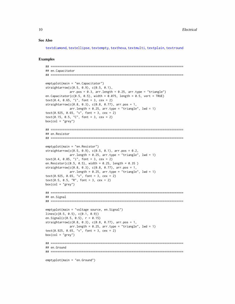
## =============================================================================## en.Capacitator## =============================================================================

emptyplot(main = "en.Capacitator")straightarrow(c(0.5, 0.9), c(0.5, 0.1),

arr.pos = 0.3, arr.length = 0.25, arr.type = "triangle")en.Capacitator(c(0.5, 0.5), width = 0.075, length = 0.5, vert = TRUE)text(0.4, 0.65, "i", font = 3, cex = 2)straightarrow(c(0.8, 0.3), c(0.8, 0.77), arr.pos = 1,

arr.length = 0.25, arr.type = "triangle", lwd = 1)text(0.925, 0.65, "v", font = 3, cex = 2)text(0.15, 0.5, "C", font = 3, cex = 2)box(col = "grey")

## =============================================================================## en.Resistor## =============================================================================

emptyplot(main = "en.Resistor")straightarrow(c(0.5, 0.9), c(0.5, 0.1), arr.pos = 0.2,

arr.length = 0.25, arr.type = "triangle", lwd = 1)text(0.4, 0.85, "i", font = 3, cex = 2)en.Resistor(c(0.5, 0.5), width = 0.25, length = 0.35 )straightarrow(c(0.8, 0.3), c(0.8, 0.77), arr.pos = 1,

arr.length = 0.25, arr.type = "triangle", lwd = 1)text(0.925, 0.65, "v", font = 3, cex = 2)text(0.5, 0.5, "R", font = 3, cex = 2)box(col = "grey")

## =============================================================================## en.Signal## =============================================================================

emptyplot(main = "voltage source, en.Signal")lines(c(0.5, 0.5), c(0.1, 0.9))en.Signal(c(0.5, 0.5), r = 0.15)straightarrow(c(0.8, 0.3), c(0.8, 0.77), arr.pos = 1,

arr.length = 0.25, arr.type = "triangle", lwd = 1)text(0.925, 0.65, "v", font = 3, cex = 2)box(col = "grey")

## =============================================================================## en.Ground## =============================================================================

emptyplot(main = "en.Ground")

Electrical 11

straightarrow(c(0.5, 0.7), c(0.5, 0.25), arr.pos = 1.0,arr.length = 0.25, arr.type = "triangle", lwd = 1)

en.Ground(c(0.5, 0.65), width = 0.25, length = 0.35 )box(col = "grey")

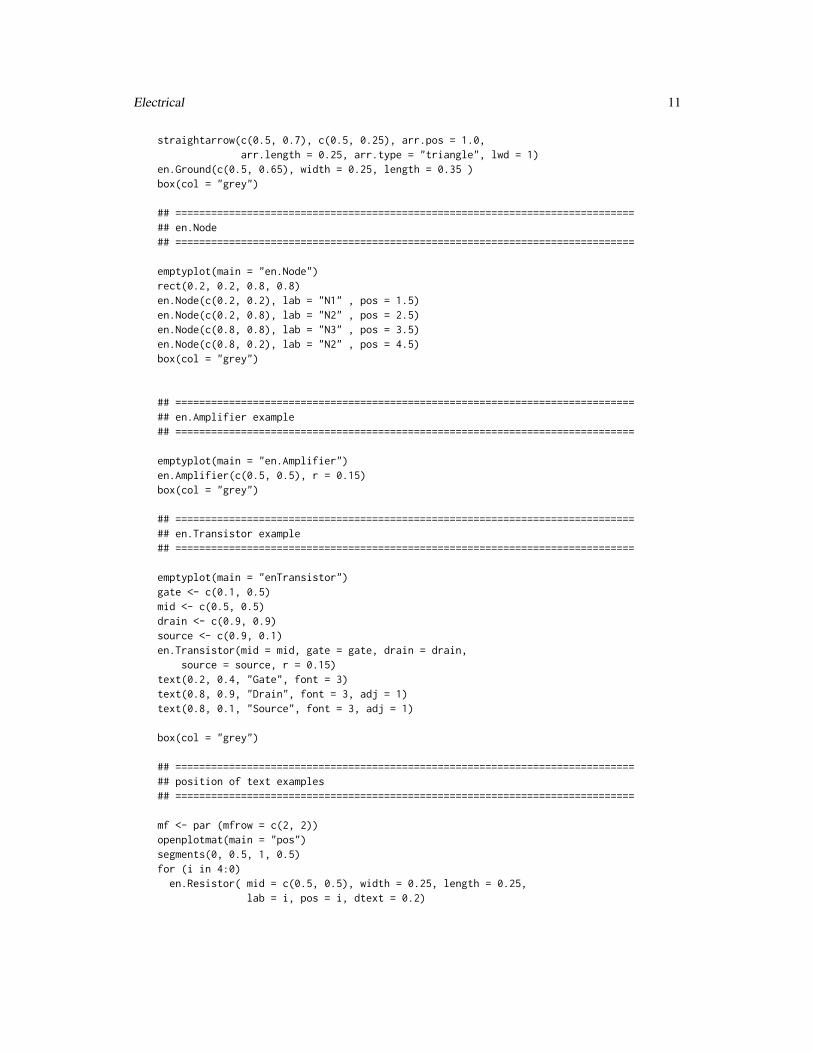
## =============================================================================## en.Node## =============================================================================

emptyplot(main = "en.Node")rect(0.2, 0.2, 0.8, 0.8)en.Node(c(0.2, 0.2), lab = "N1" , pos = 1.5)en.Node(c(0.2, 0.8), lab = "N2" , pos = 2.5)en.Node(c(0.8, 0.8), lab = "N3" , pos = 3.5)en.Node(c(0.8, 0.2), lab = "N2" , pos = 4.5)box(col = "grey")

## =============================================================================## en.Amplifier example## =============================================================================

emptyplot(main = "en.Amplifier")en.Amplifier(c(0.5, 0.5), r = 0.15)box(col = "grey")

## =============================================================================## en.Transistor example## =============================================================================

emptyplot(main = "enTransistor")gate <- c(0.1, 0.5)mid <- c(0.5, 0.5)drain <- c(0.9, 0.9)source <- c(0.9, 0.1)en.Transistor(mid = mid, gate = gate, drain = drain,

source = source, r = 0.15)text(0.2, 0.4, "Gate", font = 3)text(0.8, 0.9, "Drain", font = 3, adj = 1)text(0.8, 0.1, "Source", font = 3, adj = 1)

box(col = "grey")

## =============================================================================## position of text examples## =============================================================================

mf <- par (mfrow = c(2, 2))openplotmat(main = "pos")segments(0, 0.5, 1, 0.5)for (i in 4:0)

en.Resistor( mid = c(0.5, 0.5), width = 0.25, length = 0.25,lab = i, pos = i, dtext = 0.2)

12 Electrical

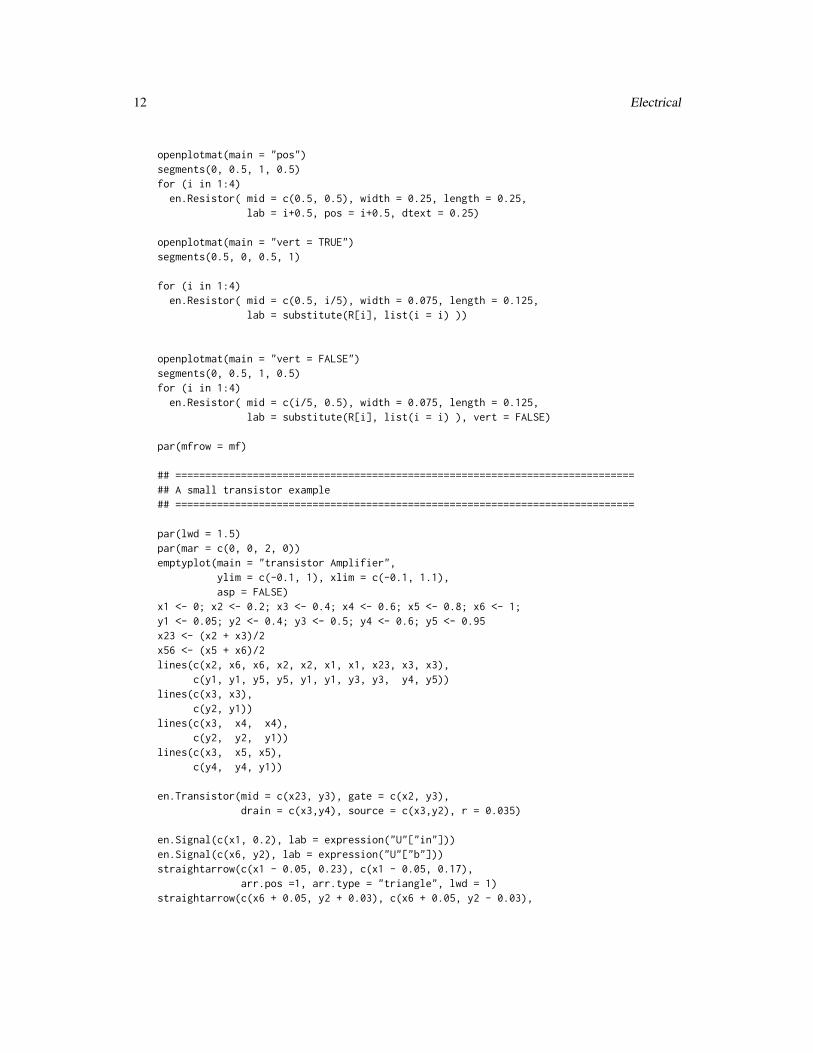
openplotmat(main = "pos")segments(0, 0.5, 1, 0.5)for (i in 1:4)

en.Resistor( mid = c(0.5, 0.5), width = 0.25, length = 0.25,lab = i+0.5, pos = i+0.5, dtext = 0.25)

openplotmat(main = "vert = TRUE")segments(0.5, 0, 0.5, 1)

for (i in 1:4)en.Resistor( mid = c(0.5, i/5), width = 0.075, length = 0.125,

lab = substitute(R[i], list(i = i) ))

openplotmat(main = "vert = FALSE")segments(0, 0.5, 1, 0.5)for (i in 1:4)

en.Resistor( mid = c(i/5, 0.5), width = 0.075, length = 0.125,lab = substitute(R[i], list(i = i) ), vert = FALSE)

par(mfrow = mf)

## =============================================================================## A small transistor example## =============================================================================

par(lwd = 1.5)par(mar = c(0, 0, 2, 0))emptyplot(main = "transistor Amplifier",

ylim = c(-0.1, 1), xlim = c(-0.1, 1.1),asp = FALSE)

x1 <- 0; x2 <- 0.2; x3 <- 0.4; x4 <- 0.6; x5 <- 0.8; x6 <- 1;y1 <- 0.05; y2 <- 0.4; y3 <- 0.5; y4 <- 0.6; y5 <- 0.95x23 <- (x2 + x3)/2x56 <- (x5 + x6)/2lines(c(x2, x6, x6, x2, x2, x1, x1, x23, x3, x3),

c(y1, y1, y5, y5, y1, y1, y3, y3, y4, y5))lines(c(x3, x3),

c(y2, y1))lines(c(x3, x4, x4),

c(y2, y2, y1))lines(c(x3, x5, x5),

c(y4, y4, y1))

en.Transistor(mid = c(x23, y3), gate = c(x2, y3),drain = c(x3,y4), source = c(x3,y2), r = 0.035)

en.Signal(c(x1, 0.2), lab = expression("U"["in"]))en.Signal(c(x6, y2), lab = expression("U"["b"]))straightarrow(c(x1 - 0.05, 0.23), c(x1 - 0.05, 0.17),

arr.pos =1, arr.type = "triangle", lwd = 1)straightarrow(c(x6 + 0.05, y2 + 0.03), c(x6 + 0.05, y2 - 0.03),

openplotmat 13

arr.pos = 1, arr.type = "triangle", lwd = 1)

en.Node(c(x1, y3), lab = "u1")en.Node(c(x2, y3), lab = "u2")en.Node(c(x3, y2), lab = "u3", pos = 1.5)en.Node(c(x3, y4), lab = "u4", pos = 2.5)en.Node(c(x5, y4), lab = "u5")

en.Capacitator(c(0.5*(x1 + x2),y3), lab = "C1", vert = FALSE)en.Capacitator(c(x4, y4), lab = "C3", vert = FALSE)en.Capacitator(c(x4, 0.5*(y1+y2)), lab = "C2", vert = TRUE)

en.Resistor(c(x1, y2), lab = "R0")en.Resistor(c(x2, 0.5*(y1+y2)), lab = "R1")en.Resistor(c(x2, 0.5*(y4+y5)), lab = "R2")en.Resistor(c(x3, 0.5*(y4+y5)), lab = "R4")en.Resistor(c(x3, 0.5*(y1+y2)), lab = "R3")en.Resistor(c(x5, 0.5*(y1+y2)), lab = "R5")

en.Ground(c(1.0, 0.05))

openplotmat Creates an empty plot used for diagram plotting.

Description

Creates a plotting region, bounded by [0,1] without axes, labels, titles

Usage

openplotmat (asp = NA, ...)

Arguments

asp the y/x aspect ratio.

... arguments passed to emptyplot from package shape.

Author(s)


See Also

emptyplot from package shape.

14 plotmat

plotmat plots a graph (network), based on a transition matrix

Description

visualises a transition matrix as a number of (labeled) boxes connected by (labeled) arrows.

Usage

plotmat(A, pos = NULL, curve = NULL, name = NULL, absent = 0,relsize = 1, lwd = 2, lcol = "black", box.size = 0.1,box.type = "circle", box.prop = 1, box.col = "white",box.lcol = lcol, box.lwd = lwd,shadow.size = 0.01, shadow.col = "grey", dr = 0.01,dtext = 0.3, self.lwd = 1, self.cex = 1,self.shiftx = box.size, self.shifty = NULL,self.arrpos = NULL, arr.lwd = lwd, arr.lcol = lcol,arr.col = "black", arr.type = "curved", arr.pos = 0.5,arr.length = 0.4, arr.width = arr.length/2,endhead = FALSE, mx = 0.0, my = 0.0, box.cex = 1,txt.col = "black", txt.xadj = 0.5, txt.yadj = 0.5,txt.font = 1, prefix = "", cex = 1, cex.txt = cex,add = FALSE, main = "", cex.main = cex,segment.from = 0, segment.to = 1, latex = FALSE, ...)

Arguments

A square coefficient matrix, specifying the links (rows=to, cols=from).

pos vector, specifying the number of elements in each graph row, or a 2-columnmatrix with element position, or NULL. If a 2-column matrix, the values shouldbe withing 0 and 1.

curve one value, or a matrix, same dimensions as A, specifying the arrow curvature; 0for straight; NA for default curvature.

name string vector, specifying the names of elements, dimension = number of rows(columns) of A.

absent all elements in A different from this value are connected.

relsize scaling factor for size of the graph.

lwd default line width of arrow and box.

lcol default color of arrow line and box line.

box.size size of label box, one value or a vector with dimension = number of rows of A.

box.type shape of label box (rect, ellipse, diamond, round, hexa, multi), one value or avector with dimension=number of rows of A.

box.prop length/width ratio of label box, one value or a vector with dimension=numberof rows of A.

plotmat 15

box.col fill color of label box, one value or a vector with dimension=number of rows ofA.

box.lcol line color of label box, one value or a vector with dimension=number of rows ofA.

box.lwd line width of the box, one value or a vector with dimension = number of rows ofA.

shadow.size relative size of shadow of label box, one value or a vector with dimension=numberof rows of A.

shadow.col color of shadow of label box, one value or a vector with dimension=number ofrows of A.

dr size of segments, in radians, to draw ellipse (decrease for smoother ellipses).

dtext controls the position of arrow text relative to arrowhead.

self.lwd line width of self-arrow, (arrow from i to i), one value or a vector with dimen-sion=number of rows of A.

self.cex relative size of self-arrow, relative to box, one value or a vector with dimen-sion=number of rows of A.

self.shiftx relative shift of self-arrow, in x-direction, one value or a vector with dimen-sion=number of rows of A.

self.shifty relative shift of self-arrow, in y-direction, one value or a vector with dimen-sion=number of rows of A.

self.arrpos position of the self-arrow, angle in radians relative to x-direction, one value or avector with dimension=number of rows of A.

arr.lwd line width of arrow, connecting two different points, one value, or a matrix withsame dimensions as A.

arr.lcol color of arrow line, one value, or a matrix with same dimensions as A.

arr.col color of arrowhead, one value, or a matrix with same dimensions as A.

arr.type type of arrowhead, one of ("curved", "triangle", "circle", "ellipse", "T", "sim-ple"), one value, or a matrix with same dimensions as A.

arr.pos relative position of arrowhead on arrow segment/curve, one value, or a matrixwith same dimensions as A.

arr.length arrow length, one value, or a matrix with same dimensions as A.

arr.width arrow width, one value, or a matrix with same dimensions as A.

endhead if TRUE: the arrow line stops at the arrowhead; default = FALSE and arrow linecontinues beyond the arrow head.

mx horizontal shift of the boxes.

my vertical shift of the boxes.

box.cex relative size of text in boxes, one value or a vector with dimension=number ofrows of A.

txt.col color of text in boxes, one value or a vector with dimension=number of rows ofA.

16 plotmat

txt.xadj, txt.yadj

the x and y adjustment of the labels in the boxes, one value or a vector withdimension=number of rows of A values usually within [0,1], although on mostdevices values outside that interval will also work.

txt.font the font to be used for the text in boxes, one value or a vector with dimen-sion=number of rows of A.

prefix to be added in front of non-zero arrow labels.cex relative size of text.cex.txt relative size of arrow text, one value, or a matrix with same dimensions as A.add start a new plot (FALSE), or add to current plot (TRUE).main main title. Only effective if add = FALSE.cex.main relative size of main title.segment.from if not 0 then the arrow line will not start at the position as given in A, but with an

offset. one value, or a matrix with same dimensions as Asegment.to if not 1 then the arrow line will not end at the position as given in A, but with an

offset. one value, or a matrix with same dimensions as Alatex if FALSE then expressions will be interpreted before print, if TRUE they will be

printed literally to the plot. Set to TRUE if LaTeX code is to be printed.... other arguments passed to function shadowbox.

Details

The square transition matrix A determines the number of elements of A (rows of A) and whichelements are connected (all values in A different from absent).

A also provides the values of arrowlabels.

The position of the elements are specified with pos, which is either NULL, or a vector specifying thenumber of elements on a row, or a 2-columned matrix specifying the (x,y) position of each element.

The ordering of elements is according to the row number of A

• when pos is NULL, the elements will be arranged on a circle• when pos is a vector, it specifies the number of elements in each row. For instance, withpos = c(3,2,1) the elements will be arranged in 3 rows (length of vector); on top row, 3elements; on second row 2, and on third row 1 element will be positioned. All elements withina row are equally distributed horizontally, all rows are equally distributed vertically.

• when pos is a matrix, it specifies the x (1st column) and y (2nd column) position of eachelement.

The offset from x-axis and from y-axis can be changed with mx and my.

The name of each element is given by vector name; this name is written in its respective box.

The relative size of this text can be changed by box.cex.

By default, a shadow is drawn, in the right-lower corner of the box.

The shadow color and relative size is specified with shadow.col and shadow.size respectively.

both can be one value (equal shadows) or a vector, specifying one value for each box shadow.

shadow.size = 0 toggles off the drawing of the shadow.

The type of the box is set with "box.type" which can take on the values:

plotmat 17

• "rect": a rectangle,

• "ellipse": an ellipse,

• "diamond": a diamond,

• "round": a rectangle with rounded left and right edges,

• "hexa": a hexagonal shape,

• "multi": a multigonal shape.

• "none" if no box is to be drawn.

The length of the box is set with box.size, the proportionality (length/width) ratio with box.prop.

The fill-color of the box is specified with box.col; the line width of the box with box.lwd and theline color with box.lcol;

All box properties can be either one value (equal boxes) or a vector, specifying one value for eachbox.

For all values A[i,j] of A which are not equal to absent, one arrow is drawn *from* column-elementj *to* the row-element i of A.

The curvature of this arrow is specified with matrix element curve[i,j],

where ’curve’ is either NULL, one value, or has the same dimension as A.

A straight arrow has curvature 0, NA (the default) chooses a default curvature,

Positive or negative values of curve draws curved arrows.

If the arrow is curved, then dr is the increment used to draw the ellipse; set to a lower value forsmoother lines.


• "simple" : uses comparable R function arrows

• "triangle": uses filled triangle

• "curved" : draws arrowhead with curved edges

• "circle" : draws circular head



The line color and width of the arrow line is set with arr.lcol and arr.lwd

The size of the arrow head is specified with arr.length and arr.width,

the position of the arrow head is specified with arr.pos (value between [0,1]).

see Arrowhead for details on arrow head

Value

a list containing:

arr a data.frame with arrow information:

• nonzero: the elements between which an arrow is drawn.• Angle: the angle of the arrow.

18 plotmat

• Value: the value written next to the arrow head.• rad: the radius of the arrow (if 0: straight line).• ArrowX: the x-position of arrowhead.• ArrowY: the y-position of arrowhead.• TextX: the x-position of arrowtext.• TextY: the y-position of arrowtext.

.

comp a matrix with the element position (centre of the boxes).

radii the radiusses in x- and y-direction of the boxes.

rect the "xleft","ybot","xright",and "ytop" of the boxes - redundant.

Author(s)


See Also

shadowbox,

Arrowhead from package shape

try: demo(plotmat)

Examples

M <- matrix(nrow = 4, ncol = 4, byrow = TRUE, data = 0)pp <- plotmat(M, pos = c(1, 2, 1), name = c("A", "B", "C", "D"),

lwd = 1, box.lwd = 2, cex.txt = 0.8,box.size = 0.1, box.type = "square", box.prop = 0.5,main = "plotmat")

pp

# when explicitly given, pos should should be inbetween 0, 1pos <- cbind (c(0.2, 0.4, 0.6, 0.8), c(0.8, 0.6, 0.4, 0.2))

pp <- plotmat(M, pos = pos, name = c("A", "B", "C", "D"),lwd = 1, box.lwd = 2, cex.txt = 0.8,box.size = 0.1, box.type = "square", box.prop = 0.5,main = "plotmat")

# includes arrows between boxespm <- par(mfrow = c(2, 2))M <- matrix(nrow = 4, ncol = 4, byrow = TRUE, data = 0)M[2, 1] <- M[3, 1] <- M[4, 2] <- M[4, 3] <- "f1"

col <- Mcol[] <- "red"col[2, 1] <- col[3, 1] <- "blue"pp <- plotmat(M, pos = c(1, 2, 1), curve = 0, name = 1:4,

lwd = 1, box.lwd = 2, box.cex = 1:4, cex.txt = 0.8,

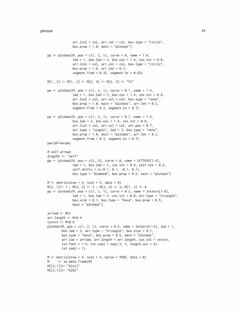
plotmat 19

arr.lcol = col, arr.col = col, box.type = "circle",box.prop = 1.0, main = "plotmat")

pp <- plotmat(M, pos = c(1, 2, 1), curve = 0, name = 1:4,lwd = 1, box.lwd = 2, box.cex = 1:4, cex.txt = 0.8,arr.lcol = col, arr.col = col, box.type = "circle",box.prop = 1.0, arr.len = 0.3,segment.from = 0.35, segment.to = 0.65)

M[1, 2] <- M[1, 3] <- M[2, 4] <- M[3, 4] <- "f2"

pp <- plotmat(M, pos = c(1, 2, 1), curve = 0.1, name = 1:4,lwd = 1, box.lwd = 2, box.cex = 1:4, cex.txt = 0.8,arr.lcol = col, arr.col = col, box.type = "none",box.prop = 1.0, main = "plotmat", arr.len = 0.2,segment.from = 0.3, segment.to = 0.7)

pp <- plotmat(M, pos = c(1, 2, 1), curve = 0.1, name = 1:4,box.lwd = 2, box.cex = 1:4, cex.txt = 0.8,arr.lcol = col, arr.col = col, arr.pos = 0.7,arr.type = "simple", lwd = 2, box.type = "none",box.prop = 1.0, main = "plotmat", arr.len = 0.2,segment.from = 0.3, segment.to = 0.7)

par(mfrow=pm)

# self arrowsdiag(M) <- "self"pp <- plotmat(M, pos = c(2, 2), curve = 0, name = LETTERS[1:4],

lwd = 1, box.lwd = 2, cex.txt = 0.8, self.cex = 0.5,self.shiftx = c(-0.1, 0.1, -0.1, 0.1),box.type = "diamond", box.prop = 0.5, main = "plotmat")

M <- matrix(nrow = 4, ncol = 4, data = 0)M[2, 1]<- 1 ; M[4, 2] <- 2 ; M[3, 4] <- 3; M[1, 3] <- 4pp <- plotmat(M, pos = c(1, 2, 1), curve = 0.2, name = letters[1:4],

lwd = 1, box.lwd = 2, cex.txt = 0.8, arr.type = "triangle",box.size = 0.1, box.type = "hexa", box.prop = 0.5,main = "plotmat")

arrlwd <- M*2arr.length <- M*0.4cextxt <- M*0.8plotmat(M, pos = c(1, 2, 1), curve = 0.2, name = letters[1:4], lwd = 1,

box.lwd = 2, arr.type = "triangle", box.size = 0.1,box.type = "hexa", box.prop = 0.5, main = "plotmat",arr.lwd = arrlwd, arr.length = arr.length, cex.txt = cextxt,txt.font = 1:4, txt.xadj = seq(-3, 3, length.out = 4),txt.yadj = 1)

M <- matrix(nrow = 4, ncol = 4, byrow = TRUE, data = 0)M <- as.data.frame(M)M[[2,1]]<- "k[si]"M[[3,1]]<- "k[N]"

20 plotweb

M[[4,2]]<- "sqrt(frac(2,3))"

names <-c(expression(lambda[12]), "?",expression(lambda[13]),expression(lambda[23]))

plotmat(M, pos = c(1, 2, 1), name = names, lwd = 1, box.lwd = 2,curve = 0, cex.txt = 0.8, box.size = 0.1, box.type = "square",box.prop = 0.5, main = "plotmat")

plotmat(M, name = letters[1:4], curve = 0, box.cex = 1:4, box.lwd = 4:1,box.size = 0.075, arr.pos = 0.7,box.col = c("lightblue", "green", "yellow", "orange"))

plotweb plots a web

Description

plots a web, based on a flow matrix

Usage

plotweb(flowmat, names = NULL, lab.size = 1.5, add = FALSE,fig.size = 1.3, main = "", sub = "", sub2 = "",log = FALSE, mar = c(2, 2, 2, 2),nullflow = NULL, minflow = NULL, maxflow = NULL,legend = TRUE, leg.digit = 5, leg.title = NULL,lcol = "black", arr.col = "black",val = FALSE, val.digit = 5, val.size = 0.6, val.col = "red",val.title = NULL, val.ncol = 1,budget = FALSE, bud.digit = 5, bud.size = 0.6,bud.title = "budget", bud.ncol = 1,maxarrow = 10, minarrow = 1, length = 0.1, dcirc = 1.2, bty = "o", ...)

Arguments

flowmat flow matrix, rows=flow *from*, columns=flow *to*.

names string vector with the names of components.

lab.size relative size of name label text.

add start a new plot (FALSE), or add to current (TRUE).

fig.size if add = FALSE: relative size of figure.

main if add = FALSE: main title.

sub if add = FALSE: sub title.

plotweb 21

sub2 ifadd = FALSE: title in bottom.log logical indicating whether to scale the flow values logarithmically.mar the figure margins.nullflow either one value or a two-valued vector; if flow < nullflow[1] or flow > nullflow[2]

(if two values): flow is assumed = 0 and the arrow is not drawn.minflow flowvalue corresponding to minimum arrow thickness.maxflow flowvalue corresponding to maximum arrow thickness.legend logical indicating whether to add a legend with arrow thickness.leg.digit nr of digits for writing legend - only if legend = TRUE.leg.title title for arrow legend, e.g to give units - only if legend =TRUE.lcol line color of arrow - not used.arr.col arrow color. One value or a matrix, with same dimensions as flowmat; if a

matrix, each arrow can have a different color.val logical indicating whether to write flow values as a legend.val.digit nr of digits for writing values - only if val =TRUE.val.size relative size for writing values - only if val =TRUE.val.col color for writing values - only if val =TRUE.val.title title for values legend - only if val =TRUE.val.ncol number of columns for writing values - only if val =TRUE.budget logical indicating whether to calculate budget (sum of flows in - sum of flows

out) per component.bud.digit nr of digits for writing budget - only if budget =TRUE.bud.size relative size for writing budget - only if budget =TRUE.bud.title title for budget legend - only if budget =TRUE.bud.ncol number of columns for writing budget - only if budget =TRUE.maxarrow maximal thickness of arrow.minarrow minimal thickness of arrow.length length of the edges of the arrow head (in inches).dcirc if cannibalism (flow from i to i), offset of circular ’arrow’ - if dcirc = 0:no circle

drawn.bty the type of box to be drawn around the legends (legend, val, budget). The

allowed values are "o" (the default) and "n".... extra arguments passed to R-function arrows.

Details

This function is less flexible than function plotmat

It is meant for visualisation of food web flows, that are inputted as a flow matrix.

It displays the elements on a circle, and, where there is a mass flow, two elements are connected,

the magnitude of the web flows is reflected by the thickness of the arrow

Note that the input matrices from function plotmat and plotweb are transposed.

22 Rigaweb

Author(s)


See Also

plotmat,

Rigaweb, Takapotoweb

try: demo(plotweb)

Examples

plotweb(Rigaweb, main = "Gulf of Riga food web",sub = "mgC/m3/d", val = TRUE)

ArrCol <- RigawebArrCol[] <- "black"ArrCol[,"Sedimentation"] <- "green"

plotweb(Rigaweb, main = "Gulf of Riga food web",sub = "mgC/m3/d", val = FALSE, arr.col = ArrCol)

plotweb(diag(20), main = "plotweb")

Rigaweb Gulf of Riga autumn planktonic food web

Description

Carbon flux matrix of the Gulf of Riga planktonic food web in autumn as reconstructed by inversemodelling by Donali et al. (1999).

The Gulf of Riga is a highly eutrophic system in the Baltic Sea.

The foodweb comprises 7 functional compartments:

• picoautotrophs (P1)• non-picoautotrophs (P2)• bacteria (B)• heterotrophic nanoflagellates (N)• zooplankton (Z)• detritus, including virus (D)• dissolved organic carbon (DOC)

and two external compartments:

• CO2• Sedimentation

These compartments are connected with 26 flows.

Units of the flows are mg C/m3/day.

segmentarrow 23

Usage

Rigaweb

Format

matrix with flow values, where element ij denotes flow from compartment i to j

rownames and columnames are the components.

Author(s)


References

Donali, E., Olli, K., Heiskanen, A.S., Andersen, T., 1999. Carbon flow patterns in the planktonicfood web of the Gulf of Riga, the Baltic Sea: a reconstruction by the inverse method. Journal ofMarine Systems 23, pp. 251 268.

See Also

Takapotoweb

Examples

plotweb(Rigaweb, main = "Gulf of Riga planktonic food web",sub = "mgC/m3/day")

segmentarrow adds 3-segmented arrow between two points.

Description

Connects two points with 3 segments (default = left-vertical-right) and adds an arrowhead on oneof the segments at a certain distance

Usage

segmentarrow(from, to, lwd = 2, lty = 1, lcol = "black",arr.col = lcol, arr.side = 2, arr.pos = 0.5,path = "LVR", dd = 0.5, ...)

24 segmentarrow

Arguments

from coordinates (x,y) of point *from* which to draw arrow.

to coordinates (x,y) of point *to* which to draw arrow.

lwd line width.

lty line type.

lcol line color.

arr.col arrow color.

arr.side segment number on which arrowhead is drawn (1,2,3).


path outline of the 3 segments, default: left, vertical, right.

dd length of segment arm, directed away from endpoints.

... arguments passed to function straightarrow.

Details

one segmented arrow is drawn between two points ’(from, to)’

how the segments are drawn is set with path which can take on the values:

• "LVR": first left then vertical then right.

• "RVL": first right then vertical then left.

• "UHD": first up then horizontal then down.

• "DHU": first down then horizontal then up.

The segment(s) on which the arrow head is drawn is set with arr.side, which is one or more valuesin (1, 2, 3).

The position of the arrowhead, on the segment on which it is drawn, is set with arr.pos, a valuebetween 0(start of segment) and 1 (end of segment)









Value


selfarrow 25

Author(s)


See Also

straightarrow, bentarrow, curvedarrow, selfarrow, treearrow, splitarrow,


Arrows: more complicated arrow function from package shape

try: demo(plotweb)

Examples

openplotmat(main="segmentarrow")

pos <-cbind(A <- seq(0.2, 0.8, by = 0.2), rev(A))


segmentarrow(from = pos[1, ] + c(0, 0.05), to = pos[2, ] + c(0, 0.05),arr.pos = 1, arr.adj = 1, dd = 0.1,path = "UHD", lcol = "darkred")

segmentarrow(from = pos[2, ] + c(-0.05, 0), to = pos[3, ] + c(-0.05, 0.01),arr.pos = 1, arr.adj = 1, dd = 0.1,lcol = "black", arr.type = "triangle")

segmentarrow(from = pos[2, ] + c(0.05, 0), to = pos[3, ] + c(0.05, 0.01),arr.pos = 0.5, dd = 0.3, path = "RVL", arr.side = 1,lcol = "lightblue", arr.type = "simple")

segmentarrow(from = pos[3, ] + c(0.05, 0), to = pos[4, ] + c(-0.05, 0.01),arr.pos = 0.5, dd = 0.05, path = "RVL", lcol = "darkblue",arr.type = "ellipse")

segmentarrow(from = pos[3, ] + c(0, -0.05), to = pos[4, ] + c(0, 0.05),arr.pos = 0.5, arr.side = 3, dd = 0.05, path = "DHU",lcol = "darkgreen")

segmentarrow(from = pos[3,] + c(-0.05, -0.05), to = pos[4, ] + c(0, -0.05),arr.pos = 0.5, arr.side = 1:3, dd = 0.3, path = "DHU",lcol = "green")

selfarrow adds a circular, self-pointing arrow to a plot

Description

adds a circular arrow, from and to the same point

26 selfarrow

Usage

selfarrow(pos, lwd = 2, lty = 1, lcol = "black", arr.pos = 0.5,path = "L", curve = c(0.1, 0.1), dr = 0.01, code = 1, ...)

Arguments

pos 2-valued vector with coordinates (x,y) of points *from and to* which to drawarrow.

lwd line width.

lty line type.

lcol line color.


path position of circle: R, L, U, D for right, left, up and down respectively.

curve relative size of curve (fraction of arrow length).


code how to put the arrowhead.


Details

draws a circular arrow from and to one point

The position of the arrowhead on the circle is set with arr.pos, a value between 0 (at start) and 1(atend of circle)








see Arrowhead for details on arrow head.

Value


Author(s)


shadowbox 27

See Also

straightarrow, segmentarrow, curvedarrow, bentarrow,treearrow, splitarrow,



Examples

openplotmat(main = "selfarrow")

pos <- coordinates(3, mx = 0.05)


for (i in 1:3)selfarrow(pos = pos[i, ], path = "R", arr.pos = 0.2,

curve = c(0.05, 0.1), lcol = "darkred")

for (i in 1:3)selfarrow(pos = pos[i, ], path = "L", arr.pos = 0.7,

lcol = "darkblue", curve = c(0.05, 0.05))

for (i in 1:3)selfarrow(pos = pos[i, ], path = "L", arr.pos = 0.5,

lcol = "darkgreen", code = i, arr.type = "triangle")

shadowbox adds a box with a shadow to a plot

Description

adds a box, with shadow on a plot; used for writing text

Usage

shadowbox(box.type = "rect", mid, radx, rady = radx,shadow.size = 0.01, shadow.col = "grey",box.col = "white", lcol = "black", lwd = 1,dr = 0.01, angle = 0, len = 1, nr = 5, rx = rady,theta = 90, ...)

Arguments

box.type shape of the box.

mid midpoint (x,y) of the box.

radx horizontal radius of the box.

rady vertical radius of the box.

28 shadowbox

shadow.size relative size of shadow.

shadow.col color of shadow.

box.col fill color of the box.

lcol line color surrounding box.

lwd line width of line surrounding the box.

dr if box is curved: size of segments, in radians, to draw ellipse (decrease forsmoother).

angle rotation angle, degrees.

len if box.type="cylinder": length of the cylinder.

nr if box.type="multi": the number of angles.

rx if box.type="round", the radius of the rounded part.

theta if box.type="parallel", angle of the bottom, left corner of the parallelogram, indegrees.

... other arguments.

Details

one box is drawn, centered aroung point mid and with horizontal and vertical radiusses radx, rady.

By default, a shadow is drawn, in the right-lower corner of the box.

The shadow color and relative size is specified with shadow.col and shadow.size respectively.

shadow.size = 0 toggles off the drawing of the shadow.

the type of the box is set with box.type which can take on the values:

• "rect": a rectangle.

• "ellipse": an ellipse.

• "diamond": a diamond.

• "round": a rectangle with rounded sides.

• "hexa": a hexagonal shape.

• "multi": a multigonal shape; also input "nr", the number of angles.

• "cylinder": a cylindrical shape; also input "len", the length of the cylinder.

• "parallel": a parallelogram; “theta” is the angle of the bottom left corner.

the fill-color of the box is specified with box.col;

the line width and color of the box are specified with lwd and lcol

Author(s)


splitarrow 29

Examples

openplotmat(main="shadowbox")

shadowbox(box.type = "rect", mid = c(0.1, 0.5),rady = 0.1, radx = 0.05, angle = 25)

shadowbox(box.type = "round", mid = c(0.3, 0.5),rady = 0.05, radx = 0.025, angle = 90,shadow.col = "darkred")

shadowbox(box.type = "ellipse", mid = c(0.5, 0.5),rady = 0.05, radx = 0.075, box.col = "blue")

shadowbox(box.type = "multi", mid = c(0.8, 0.5),rady = 0.05, radx = 0.05, box.col = "darkblue", nr = 5)

splitarrow adds a branched arrow between several points

Description

connects two sets of points with a star-like structure, adds an arrowhead at a certain distance

Usage

splitarrow(from, to, lwd = 2, lty = 1, lcol = "black", arr.col = lcol,arr.side = 2, arr.pos = 0.5, centre = NULL, dd = 0.5, ...)

Arguments

from matrix of coordinates (x,y) of points *from* which to draw arrow.

to matrix of coordinates (x,y) of points *to* which to draw arrow.

lwd line width.

lty line type.

lcol line color.




centre coordinates (x,y) of central point.

dd relative position of central point, only when centre=NULL.


30 splitarrow

Details

a branched arrow is drawn between points ’(from, to)’, where both from and to can be severalpoints.

The arrow segments radiate into a central point. Either the (x,y) coordinates of this central pointare set with centre or it is estimated at a certain distance (dd >0,<1) between the centroid of the*from* points and the centroid of the *to* points.


• arr.side=1 sets the arrow head on the segment *from* -> central point

• arr.side=2 sets the arrow head on the segment central point -> *to*

The position of the arrowhead on the segment on which it is drawn, is set with arr.pos, a valuebetween 0(start of segment) and 1(end of segment)









Value

coordinates (x,y) where arrowheads are drawn

Author(s)


See Also

straightarrow, segmentarrow, curvedarrow, selfarrow, bentarrow, treearrow,



Examples

openplotmat(main = "splitarrow")

pos <- coordinates(c(1, 2, 2, 4, 1))splitarrow(from = pos[1, ], to = pos[2:10, ],

arr.side = 1, centre = c(0.5, 0.625))for (i in 1:10)

straightarrow 31

textrect(pos[i, ], lab = i, cex = 2, radx = 0.05)

openplotmat(main = "splitarrow")

pos <- coordinates(c(1, 3))splitarrow(from = pos[1,], to = pos[2:4, ], arr.side = 1)splitarrow(from = pos[1,], to = pos[2:4, ], arr.side = 2)for (i in 1:4)


openplotmat(main = "splitarrow")pos <- coordinates(N = 6)pos <- rbind(c(0.5, 0.5), pos)splitarrow(from = pos[1, ], to = pos[2:7, ], arr.side = 2)for (i in 1:7)


straightarrow adds straight arrow between two points

Description

Plots straight line between two points

adds an arrowhead at a certain distance.

Usage

straightarrow(from, to, lwd = 2, lty = 1, lcol = "black",arr.col = lcol, arr.pos = 0.5, endhead = FALSE,segment = c(0,1), ...)

Arguments



lwd line width.

lty line type.

lcol line color.



endhead if TRUE: the arrow line stops at the arrowhead; default = FALSE.

segment if not c(0,1): then the arrow line will cover only part of the requested path, e.g.if segment = c(0.2,0.8), it will start 0.2 from from and till 0.8.


32 straightarrow

Details

a straight arrow is drawn between the points ’(from, to)’ The position of the arrowhead, is set witharr.pos, a value between 0(start point) and 1(endpoint)









Value


Author(s)


See Also

bentarrow, segmentarrow, curvedarrow selfarrow, splitarrow, treearrow,



Examples

openplotmat(main = "straightarrow")

pos <- coordinates(c(2, 3, 1))

for (i in 1:5)straightarrow(from = pos[i, ], to = pos[i+1, ], arr.pos = 0.5)

straightarrow(from = pos[6, ], to = pos[6, ] + c(0.3, 0.),arr.type = "T", arr.pos = 1, arr.lwd = 3)

for (i in 1:6)textrect(pos[i, ], lab = LETTERS[i], radx = 0.05)

Takapotoweb 33

Takapotoweb Takapoto atoll planktonic food web

Description

Carbon flux matrix of the Takapoto atoll planktonic food web

as reconstructed by inverse modelling by Niquil et al. (1998).

The Takapoto Atoll lagoon is located in the French Polynesia of the South Pacific

The food web comprises 7 functional compartments:

• Phytoplankton

• Bacteria

• Protozoa

• Microzooplankton

• Mesozooplankton

• Detritus

• Dissolved organic carbon (DOC)

and three external compartments/sinks:

• CO2

• Sedimentation

• Grazing

These compartments are connected with 32 flows. Units of the flows are mg C/m2/day

Usage

Takapotoweb

Format

matrix with flow values, where element ij denotes flow from compartment i to j

rownames and columnames are the components.

Author(s)


References

Niquil, N., Jackson, G.A., Legendre, L., Delesalle, B., 1998. Inverse model analysis of the plank-tonic food web of Takapoto Atoll (French Polynesia). Marine Ecology Progress Series 165, pp. 1729.

34 Teasel

See Also

Rigaweb

Examples

plotweb(Takapotoweb, main = "Takapoto atoll planktonic food web",sub = "mgC/m2/day", lab.size = 1)

Teasel Population dynamics model transition matrix of teasel

Description

Transition matrix of the population dynamics model of teasel (Dipsacus sylvestris), a Europeanperennial weed, as discussed in Caswell (2001), and in Soetaert and Herman, (2009)

The life cycle of teasel can be described by six stages:

• dormant seeds < 1yr (DS 1yr)

• dormant seeds 1-2yr (DS 2yr)

• small rosettes <2.5cm (R small)

• medium rosettes 2.5-18.9 cm (R medium)

• large rosettes >19 cm (R large)

• flowering plants (F)

The matrix contains the transition probabilities from one compartment (column) to another (row).

Usage

Teasel

Format

matrix with transition probabilities, where element ij denotes transition from compartment j to i

rownames and columnames are the component names

Author(s)


References

Caswell, H. 2001. Matrix population models: construction, analysis, and interpretation. Secondedition. Sinauer, Sunderland, Mass.

Karline Soetaert and Peter Herman. 2009. A practical guide to ecological modelling. Using R as asimulation platform. Springer.

textdiamond 35

See Also

Rigaweb, Takapotoweb

Examples

curves <- matrix(nrow = ncol(Teasel), ncol = ncol(Teasel), 0)curves[3,1] <- curves[1,6] <- -0.35curves[4,6] <- curves[6,4] <- curves[5,6] <- curves[6,5] <- 0.08curves[3,6] <- 0.35

plotmat(Teasel, pos = c(3, 2, 1), curve = curves, lwd = 1, box.lwd = 2,cex.txt = 0.8, box.cex = 0.8, box.size = 0.08, arr.length = 0.5,box.type = "circle", box.prop = 1, shadow.size = 0.01,self.cex = 0.6, my = -0.075, mx = -0.01, relsize = 0.9,self.shifty = 0, self.shiftx = c(0, 0, 0.125, -0.12, 0.125, 0),main = "Dispsacus sylvestris")

textdiamond adds lines of text in a diamand-shaped box to a plot

Description

adds one or more lines of text, in a diamond-shaped box.

Usage

textdiamond(mid, radx, rady = NULL, lwd = 1, shadow.size = 0.01,adj = c(0.5,0.5), lab = "", box.col = "white",lcol = "black", shadow.col = "grey", angle = 0, ...)

Arguments






adj text adjustment.

lab one label or a vector string of labels to be added in box.





... other arguments passed to function textplain.

36 textellipse

Details

see shadowbox for specifications of the diamond-shaped box and its shadow.

Author(s)


See Also

textellipse, textempty,texthexa, textmulti, textplain, textrect, textround

Examples

openplotmat(xlim = c(-0.1, 1.1), main = "textdiamond")

for (i in 1:10)textdiamond(mid = runif(2), col = i, radx = 0.1, rady = 0.05,

lab = LETTERS[i], cex = 2, angle = runif(1)*360)

textellipse adds lines of text in an ellipsoid box to a plot

Description

adds one or more lines of text, centered around "mid" in an ellipsoid box

Usage

textellipse(mid, radx, rady = radx*length(lab), lwd = 1,shadow.size = 0.01, adj = c(0.5, 0.5), lab = "",box.col = "white", lcol = "black", shadow.col = "grey",angle = 0, dr = 0.01, ...)

Arguments











textempty 37




Details

see shadowbox for specifications of the ellipsoid-shaped box and its shadow

Author(s)


See Also

textdiamond, textempty, texthexa, textmulti, textplain, textrect, textround

Examples

openplotmat(xlim = c(-0.1, 1.1), main = "textellipse")

for (i in 1:10)textellipse(mid = runif(2), col = i, box.col = grey(0.95),

radx = 0.1, rady = 0.05, lab = LETTERS[i],cex = 2, angle = runif(1)*360)

textempty adds lines of text, on a colored background to a plot

Description

adds one or more lines of text, with a colored background, no box

Usage

textempty(mid, lab = "", adj = c(0.5, 0.5),box.col = "white", cex = 1, ...)

Arguments

mid midpoint (x,y) of the text.



box.col background color.

cex relative size of text.


38 texthexa

Author(s)


See Also

textdiamond, textellipse, texthexa, textmulti, textplain, textrect, textround

Examples

openplotmat(xlim = c(-0.1, 1.1), col = "lightgrey", main = "textempty")

for (i in 1:10)textempty(mid = runif(2), box.col = i, lab = LETTERS[i], cex = 2)

textempty(mid = c(0.5, 0.5), adj = c(0, 0),lab = "textempty", box.col = "white")

texthexa adds lines of text in an hexagonal box to a plot

Description

adds one or more lines of text, centered around "mid" in an hexagonal box.

Usage

texthexa(mid, radx, rady = radx*length(lab), lwd = 1,shadow.size = 0.01, adj = c(0.5,0.5),lab = "", box.col = "white", lcol = "black",shadow.col = "grey", angle = 0, ...)

Arguments













textmulti 39

Details

see shadowbox for specifications of the hexangular box and its shadow

Author(s)


See Also

textdiamond, textellipse, textempty, textmulti, textplain, textrect, textround

Examples

openplotmat(xlim = c(-0.1, 1.1), main = "texthexa")

for (i in 1:20)texthexa(mid = runif(2), angle = runif(1)*360, col = i,

box.col = grey(0.95), radx = 0.1, rady = 0.05,lab = LETTERS[i], cex = 2)

textmulti adds lines of text in an multigonal box to a plot

Description

adds one or more lines of text, centered around "mid" in an multigonal box

Usage

textmulti(mid, radx, rady = radx*length(lab), lwd = 1,shadow.size = 0.01, adj = c(0.5, 0.5),lab = "", box.col = "white", lcol = "black",shadow.col = "grey", angle = 0, nr = 6, ...)

Arguments










40 textplain



nr the number of angles.


Details

see shadowbox for specifications of the multigonal box and its shadow.

Author(s)


See Also

textdiamond, textellipse, textempty, texthexa, textplain, textrect, textround.

Examples

openplotmat(xlim = c(-0.1, 1.1), main = "textmulti")

for (i in 1:10)textmulti(mid = runif(2), col = i, radx = 0.1, rady = 0.1,

lab = LETTERS[i], cex = 2, nr = trunc(i/1.5)+3)

textplain adds lines of text to a plot

Description

adds one or more lines of text, centered around "mid"

Usage

textplain(mid, height = 0.1, lab = "", adj = c(0.5, 0.5), ...)

Arguments

mid central coordinates where to write the text.

height height of text.

lab one or more character strings or expressions specifying the *text* to be written.

adj label adjustments.

... other arguments passed to R-function text.

Author(s)


textrect 41

See Also

textdiamond, textellipse, textempty, texthexa, textmulti, textrect, textround

Examples

openplotmat(main = "textplain")textplain(mid = c(0.5, 0.5),

lab = c("this text is", "centered", "4 strings", "on 4 lines"))textplain(mid = c(0.5, 0.2), adj = c(0, 0.5), font = 2, height = 0.05,

lab = c("this text is","left alligned"))textplain(mid = c(0.5, 0.8), adj = c(1, 0.5), font = 3, height = 0.05,

lab = c("this text is","right alligned"))

textrect adds lines of text in a rectangular-shaped box or in a parallelogram toa plot

Description

Adds one or more lines of text, centered around "mid" in a rectangular box, or in a paralellogram

Usage

textrect(mid, radx, rady = radx*length(lab), lwd = 1,shadow.size = 0.01, adj = c(0.5, 0.5),lab = "", box.col = "white",lcol = "black", shadow.col = "grey", angle = 0, ...)

textparallel (mid, radx, rady = radx*length(lab), lwd = 1,shadow.size = 0.01, adj = c(0.5, 0.5),lab = "", box.col = "white",lcol = "black", shadow.col = "grey",angle = 0, theta = 90, ...)

Arguments










42 textround



theta angle of the bottom, left corner of the parallelogram, in degrees.


Details

see shadowbox for specifications of the rectangular box and its shadow.

Author(s)


Thanks to Michael Folkes for the code of the parallelogram.

See Also

textdiamond, textellipse, textempty, texthexa, textmulti, textplain, textround

Examples

openplotmat(xlim = c(-0.1, 1.1), main = "textrect")for (i in 1:10)

textrect(mid = runif(2), col = i, radx = 0.1, rady = 0.1,lab = LETTERS[i], cex = 2)

openplotmat(xlim = c(-0.1, 1.1), main = "textparallel")elpos <-coordinates (c(1, 1, 1, 1, 1))

textparallel(mid = elpos[1,], col = 1, radx = 0.2, rady = 0.1,lab = "theta=20", theta = 20)





textround adds lines of text in a rounded box to a plot

Description

adds one or more lines of text, centered around "mid" in an a rectangular box with rounded sides

textround 43

Usage

textround(mid, radx, rady = radx*length(lab), lwd = 1,shadow.size = 0.01, adj = c(0.5, 0.5), lab = "", box.col = "white",lcol = "black", shadow.col = "grey", angle = 0, rx = rady, ...)

Arguments












rx the radius of the rounded part.


Details

see shadowbox for specifications of the box and its shadow

Author(s)


See Also

textdiamond, textellipse, textempty, texthexa, textmulti, textplain, textrect.

Examples

openplotmat(xlim = c(-0.1, 1.1), main = "textround")

for (i in 1:10)textround(mid = runif(2), col = i,

radx = 0.03, rady = 0.075,lab = LETTERS[i], cex = 2)

44 treearrow

treearrow adds a dendrogram-like branched arrow between several points

Description

connects two sets of points with a dendrogram-like structure,

adds an arrowhead at a certain distance.

Usage

treearrow(from, to, lwd = 2, lty = 1, lcol = "black", arr.col = lcol,arr.side = 2, arr.pos = 0.5, line.pos = 0.5, path = "H", ...)

Arguments

from matrix of coordinates (x,y) of points *from* which to draw arrow.

to matrix of coordinates (x,y) of points *to* which to draw arrow.

lwd line width.

lty line type.

lcol line color.




line.pos relative position of (horizontal/vertical) line.

path Vertical, Horizontal.


Details

a tree-shaped arrow is drawn between points ’(from, to)’, where both from and to can be severalpoints.

How the segments are drawn is set with path which can take on the values:

• "H": (horizontal): first left or right.

• "V": (vertical): first down- or upward.


The position of the arrowhead on the segment on which it is drawn, is set with arr.pos, a valuebetween 0(start of segment) and 1(end of segment)



treearrow 45







Value


Author(s)


See Also

straightarrow, segmentarrow, curvedarrow, selfarrow, bentarrow, splitarrow,



Examples

openplotmat(main = "treearrow")pos <- coordinates(c(3, 2, 4, 1))treearrow(from = pos[1:5, ], to = pos[6:10, ])for (i in 1:10)


openplotmat(main = "treearrow")pos <- coordinates(c(2, 4), hor = FALSE)treearrow(from = pos[1:2, ], to = pos[3:6, ],

arr.side = 1:2, path = "V")for (i in 1:6)


openplotmat(main = "treearrow")pos <- coordinates(c(3, 5, 7, 7, 5, 3))treearrow(from = pos[1:15, ], to = pos[15:30, ], arr.side = 0)for (i in 1:30)

textrect(pos[i, ], lab = i, cex = 1.2, radx = 0.025)

Index

∗Topic aplotbentarrow, 3curvedarrow, 7Electrical, 8plotmat, 14plotweb, 20segmentarrow, 23selfarrow, 25shadowbox, 27splitarrow, 29straightarrow, 31textdiamond, 35textellipse, 36textempty, 37texthexa, 38textmulti, 39textplain, 40textrect, 41textround, 42treearrow, 44

∗Topic datasetsRigaweb, 22Takapotoweb, 33Teasel, 34

∗Topic hplotopenplotmat, 13

∗Topic manipcoordinates, 5

∗Topic packagediagram-package, 2

Arrowhead, 4, 8, 17, 18, 24, 26, 30, 32, 45Arrows, 5, 7, 8, 25, 27, 30–32, 45arrows, 5, 8, 21, 24–27, 30, 32, 44, 45

bentarrow, 3, 3, 8, 25, 27, 30, 32, 45

coordinates, 3, 5curvedarrow, 3, 5, 7, 25, 27, 30, 32, 45

diagram (diagram-package), 2

diagram-package, 2

Electrical, 8en.Amplifier, 3en.Amplifier (Electrical), 8en.Capacitator, 3en.Capacitator (Electrical), 8en.Ground, 3en.Ground (Electrical), 8en.Node, 3en.Node (Electrical), 8en.Resistor, 3en.Resistor (Electrical), 8en.Signal, 3en.Signal (Electrical), 8en.Transistor (Electrical), 8

openplotmat, 3, 13

plotmat, 3, 14, 21, 22plotweb, 3, 20

Rigaweb, 22, 22, 34, 35

segmentarrow, 3, 5, 8, 23, 27, 30, 32, 45selfarrow, 3, 5, 8, 25, 25, 30, 32, 45shadowbox, 3, 18, 27, 36, 37, 39, 40, 42, 43splitarrow, 3, 5, 8, 25, 27, 29, 32, 45straightarrow, 3, 5, 8, 24, 25, 27, 29, 30, 31,

44, 45

Takapotoweb, 22, 23, 33, 35Teasel, 34text, 40textdiamond, 3, 10, 35, 37–43textellipse, 3, 10, 36, 36, 38–43textempty, 3, 10, 36, 37, 37, 39–43texthexa, 3, 10, 36–38, 38, 40–43textmulti, 10, 36–39, 39, 41–43textparallel (textrect), 41textplain, 3, 10, 35–40, 40, 42, 43

46

INDEX 47

textrect, 3, 36–41, 41, 43textround, 3, 10, 36–42, 42treearrow, 3, 5, 8, 25, 27, 30, 32, 44

package ‘diagram’ - the comprehensive r archive … for the book ``a practical guide to...

Documents