pacific ecoinformatics and computational ecology lab ......fish base server. itis taxonomy server...
TRANSCRIPT
Ilmi Yoon1,2, Sangyuk (Paul) Yoon1, Gary Ng2, Hunvil Rodrigues2, Sonal Mahajan2, and Neo D. Martinez1
1Pacific Ecoinformatics and Computational Ecology Lab,
Berkeley, California, USA
2Computer Science Department, San Francisco State University, San Francisco, California, USA
Rich J. Williams
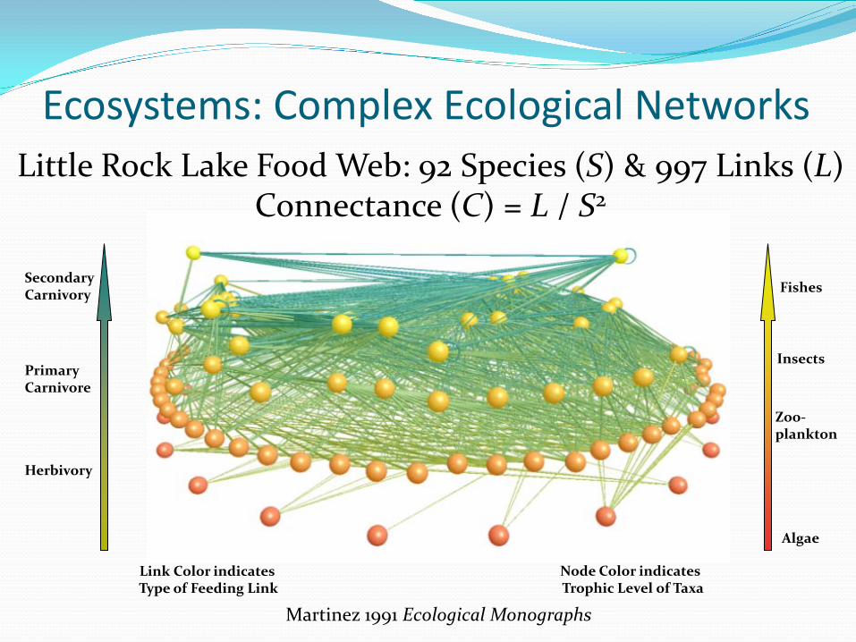
Ecosystems: Complex Ecological Networks Little Rock Lake Food Web: 92 Species (S) & 997 Links (L)
Connectance (C) = L / S2
Fishes
Insects
Zoo- plankton
Algae
Node Color indicates Trophic Level of Taxa
Secondary Carnivory
Primary Carnivore
Herbivory
Link Color indicates Type of Feeding Link
Martinez 1991 Ecological Monographs
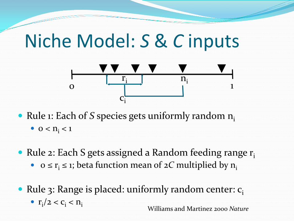
Niche Model: S & C inputs
Rule 1: Each of S species gets uniformly random ni 0 < ni < 1
Rule 2: Each S gets assigned a Random feeding range ri
0 ≤ ri ≤ 1; beta function mean of 2C multiplied by ni
Rule 3: Range is placed: uniformly random center: ci
ri/2 < ci < ni
1 0 ni
ci
Williams and Martinez 2000 Nature
ri
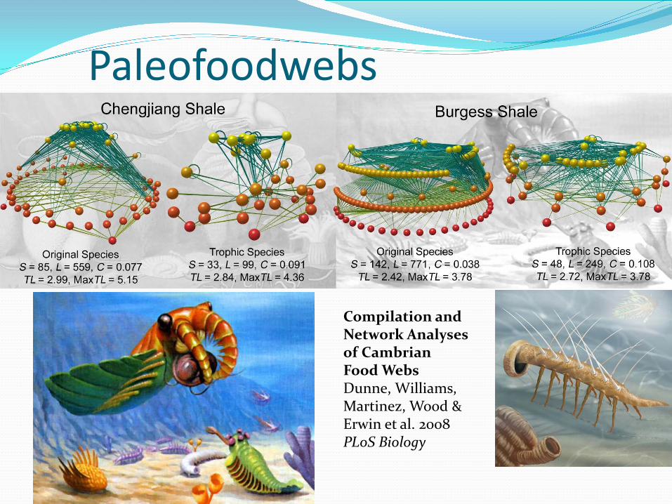
Paleofoodwebs
Compilation and Network Analyses of Cambrian Food Webs Dunne, Williams, Martinez, Wood & Erwin et al. 2008 PLoS Biology
Niche Model Generates Realistic Network Architectures
Effects of S and C on network structure
Provides a Benchmark
Scaffolding for Network Dynamics
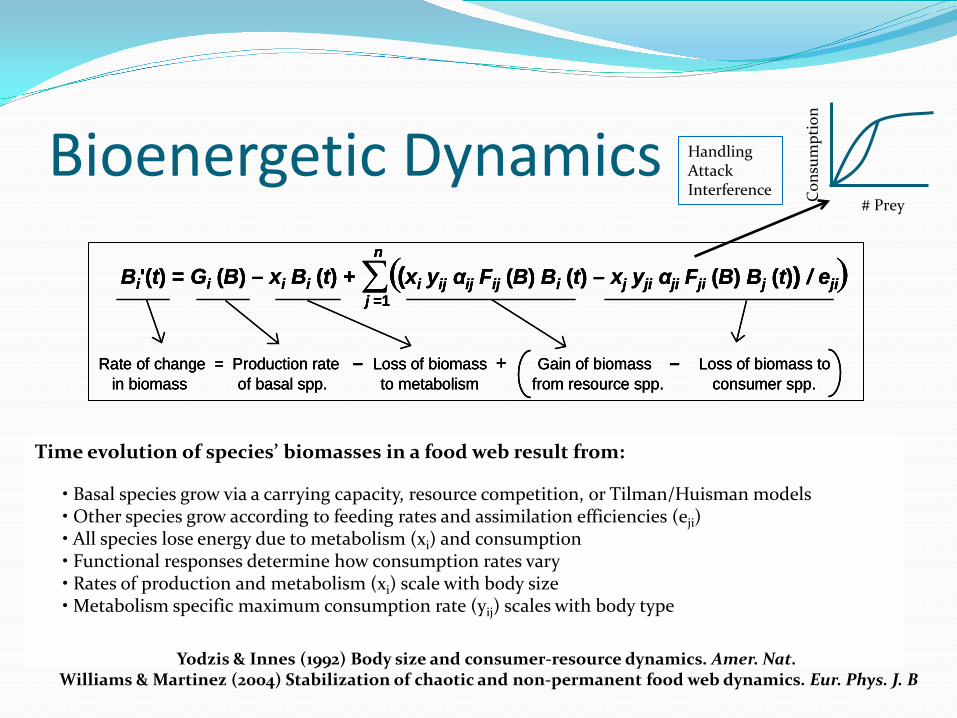
Bioenergetic Dynamics
( )∑n
j =1Bi'(t) = Gi (B) – xi Bi (t) + (xi yij αij Fij (B) Bi (t) – xj yji αji Fji (B) Bj (t)) / eji
Rate of change = Production rate – Loss of biomass + Gain of biomass – Loss of biomass to in biomass of basal spp. to metabolism from resource spp. consumer spp.
( )∑n
j =1Bi'(t) = Gi (B) – xi Bi (t) + (xi yij αij Fij (B) Bi (t) – xj yji αji Fji (B) Bj (t)) / eji( )∑
n
j =1Bi'(t) = Gi (B) – xi Bi (t) + (xi yij αij Fij (B) Bi (t) – xj yji αji Fji (B) Bj (t)) / eji
Rate of change = Production rate – Loss of biomass + Gain of biomass – Loss of biomass to in biomass of basal spp. to metabolism from resource spp. consumer spp.
Rate of change = Production rate – Loss of biomass + Gain of biomass – Loss of biomass to in biomass of basal spp. to metabolism from resource spp. consumer spp.
Time evolution of species’ biomasses in a food web result from:
• Basal species grow via a carrying capacity, resource competition, or Tilman/Huisman models • Other species grow according to feeding rates and assimilation efficiencies (eji) • All species lose energy due to metabolism (xi) and consumption • Functional responses determine how consumption rates vary • Rates of production and metabolism (xi) scale with body size • Metabolism specific maximum consumption rate (yij) scales with body type
# Prey Con
sum
ptio
n
Handling Attack Interference
Yodzis & Innes (1992) Body size and consumer-resource dynamics. Amer. Nat. Williams & Martinez (2004) Stabilization of chaotic and non-permanent food web dynamics. Eur. Phys. J. B
-1 0 1 2 3
Log
(| per
cap
ita I|
)
-4
-3
-2
-1
0
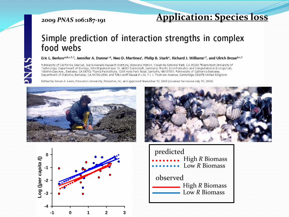
predicted
Low R Biomass High R Biomass
Low R Biomass High R Biomass
observed
2009 PNAS 106:187-191 Application: Species loss
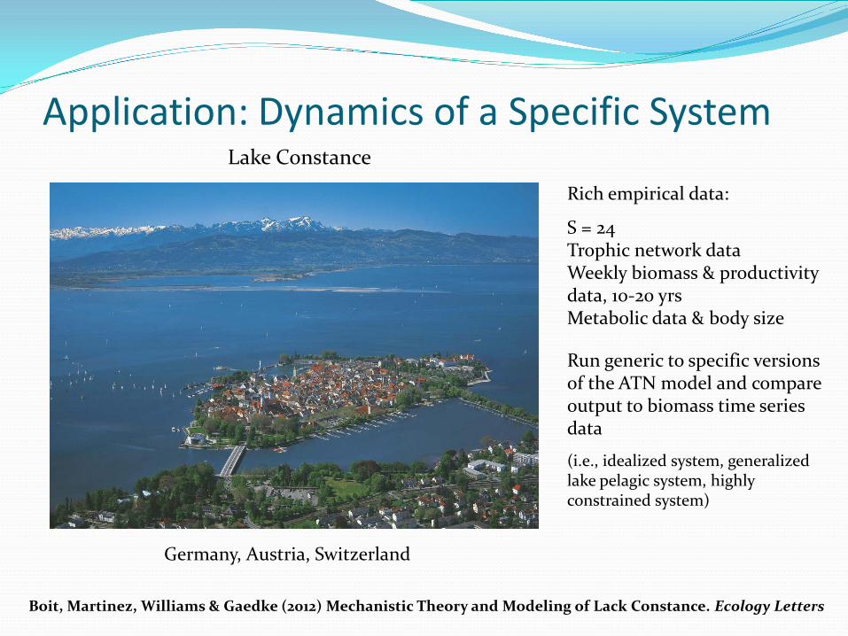
Application: Dynamics of a Specific System Lake Constance
Germany, Austria, Switzerland
Rich empirical data:
S = 24 Trophic network data Weekly biomass & productivity data, 10-20 yrs Metabolic data & body size Run generic to specific versions of the ATN model and compare output to biomass time series data
(i.e., idealized system, generalized lake pelagic system, highly constrained system)
Boit, Martinez, Williams & Gaedke (2012) Mechanistic Theory and Modeling of Lack Constance. Ecology Letters

Lake Constance 24 Species, 104 Links, Conectance = 0.18
Fish2
Lep
Fish3
Fish4
Cyc
Alg2
HNF
Rot2 Rot1
Rot3
Cru
Cil2
Alg5 APP Alg3 Alg4 Alg1
Cil1
Bac
Cil4
Cil5
Cil3
Fish1
Asp
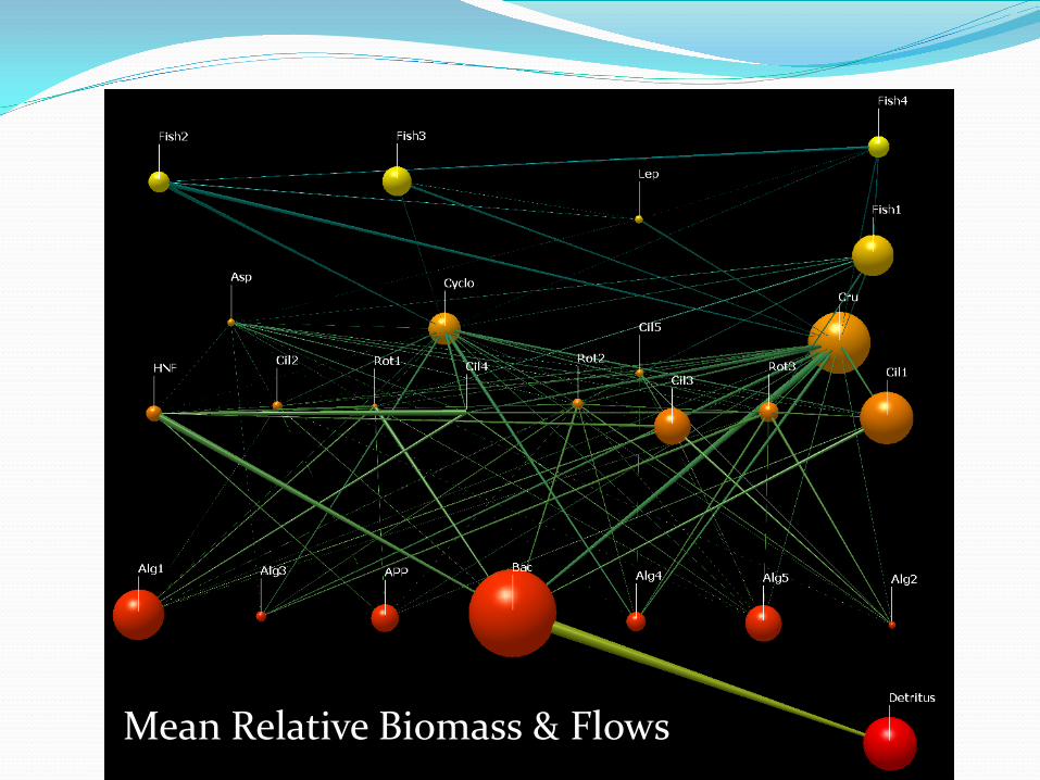
Mean Relative Biomass & Flows

1 2 3
4
5 6 7
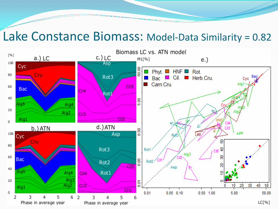
Lake Constance Biomass: Model-Data Similarity = 0.82

Ecological Forecasting Parameterize Network Model for System of Interest
Network Structure Body Size and Type
Tune Parameters to Historical Record
Update Model with Realtime Data
Continue machine learning
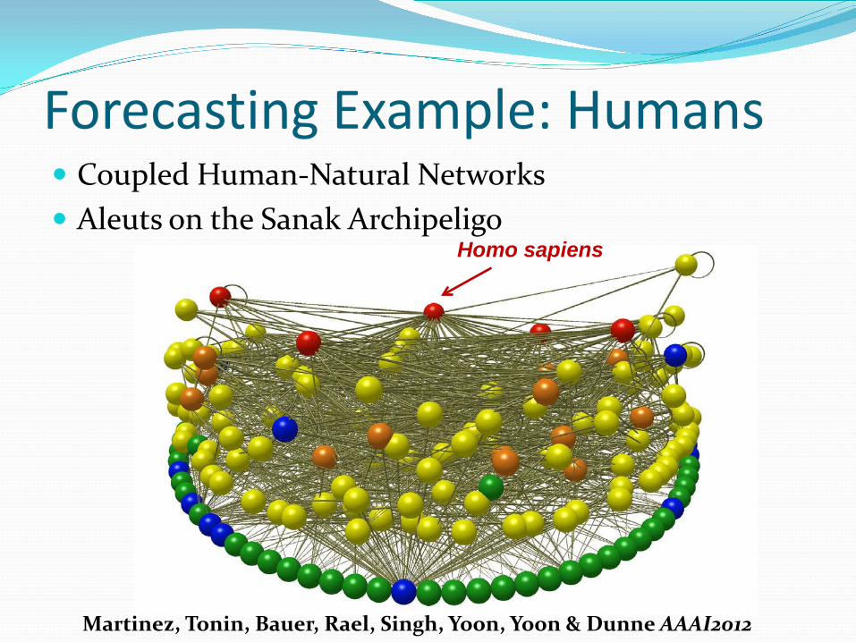
Homo sapiens
Forecasting Example: Humans Coupled Human-Natural Networks Aleuts on the Sanak Archipeligo
Martinez, Tonin, Bauer, Rael, Singh, Yoon, Yoon & Dunne AAAI2012
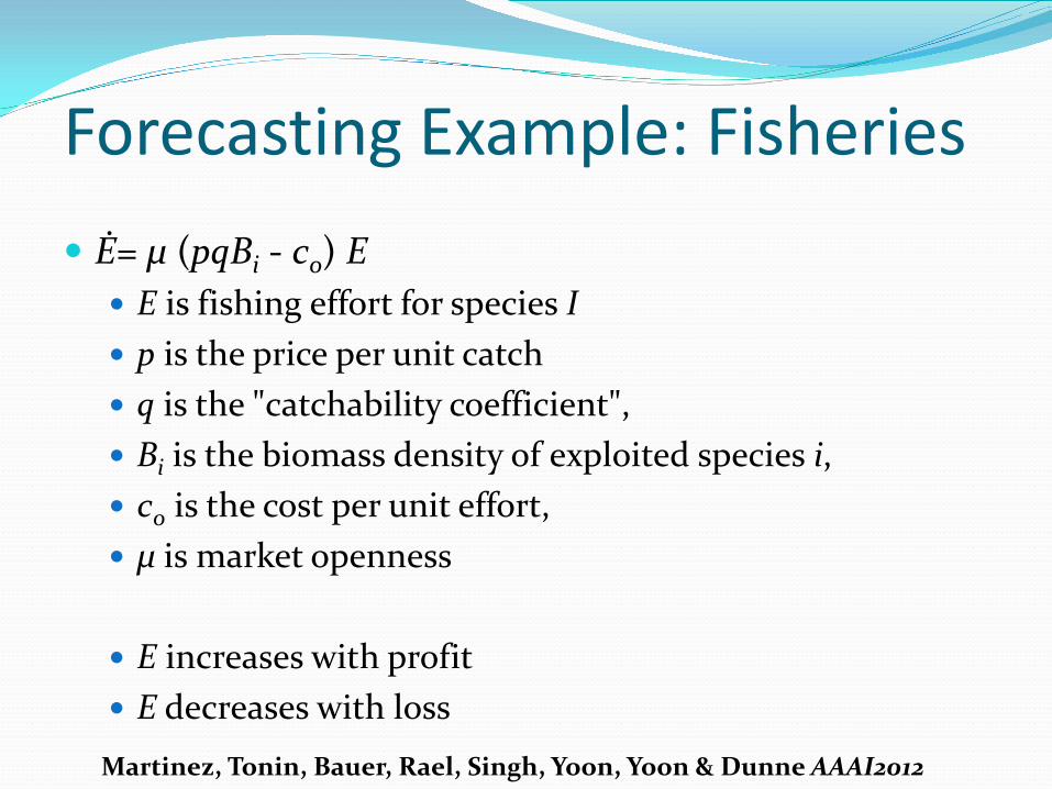
Ė= μ (pqBi - co) E E is fishing effort for species I p is the price per unit catch q is the "catchability coefficient", Bi is the biomass density of exploited species i, c0 is the cost per unit effort, μ is market openness
E increases with profit E decreases with loss
Forecasting Example: Fisheries
Martinez, Tonin, Bauer, Rael, Singh, Yoon, Yoon & Dunne AAAI2012

Forecasting Example: Fisheries
Martinez, Tonin, Bauer, Rael, Singh, Yoon, Yoon & Dunne AAAI2012

Forecasting Example: Fisheries
Martinez, Tonin, Bauer, Rael, Singh, Yoon, Yoon & Dunne AAAI2012

Cyberinfrastructure: Network3D

Fish Base Server
ITIS Taxonomy Server Server … Other servers
Client Browser
Network3D plug-in module
Web Service
Network3D on Azure Cloud Computing
MS Data Center
Network3DFramework
HTTP/HTTPS
Internet
Internet
Access Control
Network3DPopulation Dynamics
Network3D REST WCF
Service
World of Balance Server
Internet
Network3D Client program Proxy Interface
Network3D module
Query Request
Query Response
Internet WCF Proxy
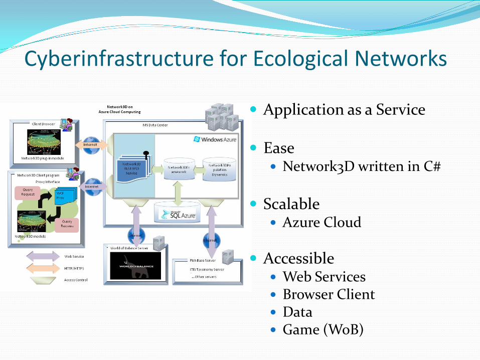
Cyberinfrastructure for Ecological Networks
Application as a Service
Ease Network3D written in C#
Scalable
Azure Cloud
Accessible Web Services Browser Client Data Game (WoB)
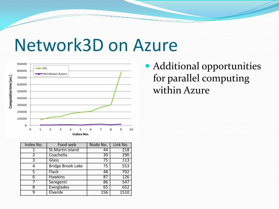
Network3D on Azure Additional opportunities
for parallel computing within Azure
0
10000
20000
30000
40000
50000
60000
70000
80000
90000
0 1 2 3 4 5 6 7 8 9 10
Com
puta
tion t
ime (
sec.)
Index No.
PC
Windows Azure
Index No. Food web Node No. Link No. 1 St.Martin Island 44 218 2 Coachella 30 290 3 Glass 75 113 4 Bridge Brook Lake 75 553 5 Flack 48 702 6 Hawkins 87 126 7 Seregenti 86 547 8 Everglades 65 652 9 Elverde 156 1510

WoB: World of Balance


Games and Research Simulations Easy to conduct Results Stored and Accessible Computer Science
Integration with other Data Empirical Observations (e.g., L. Constance, Fisheries) Other simulations (e.g., Matlab) Realtime observations (e.g., light and rain measures)
Solutions Obtained Behavior, Stability and Robustness of Ecological Networks Understanding and management of Human-Natural
Networks Social Networks/Public Appreciation of Ecosystems
Ecological and Economic Interdependence One’s own “place in the world”
Games and Research Simulations Easy to conduct Results Stored and Accessible Computer Science
Integration with other Data Empirical Observations (e.g., L. Constance, Fisheries) Other simulations (e.g., Matlab) Realtime observations (e.g., light and rain measures)
Solutions Obtained Behavior, Stability and Robustness of Ecological Networks Understanding and management of Human-Natural Networks Social Networks/Public Appreciation of Ecosystems
Ecological and Economic Interdependence/ One’s “place in the world”