p. y. foucher et al- technical note: feasibility of co2 profile retrieval from limb viewing solar...
TRANSCRIPT
8/2/2019 P. Y. Foucher et al- Technical Note: Feasibility of CO2 profile retrieval from limb viewing solar occultation made by t…
http://slidepdf.com/reader/full/p-y-foucher-et-al-technical-note-feasibility-of-co2-profile-retrieval-from 1/18
Atmos. Chem. Phys., 9, 2873–2890, 2009
www.atmos-chem-phys.net/9/2873/2009/
© Author(s) 2009. This work is distributed under
the Creative Commons Attribution 3.0 License.
AtmosphericChemistry
and Physics
Technical Note: Feasibility of CO2 profile retrieval from limb
viewing solar occultation made by the ACE-FTS instrument
P. Y. Foucher1, A. Chedin1, G. Dufour2, V. Capelle1, C. D. Boone3, and P. Bernath3,4
1Laboratoire de Meteorologie Dynamique/Institut Pierre Simon Laplace, Ecole Polytechnique, 91128 Palaiseau, France2Laboratoire Inter-universitaire des Systemes Atmospheriques, Faculte des Sciences et Technologies, 61 avenue du General
de Gaulle, 94010 Creteil, France3Department of Chemistry, University of Waterloo, Ontario, N2L3G1, Canada4Department of Chemistry, University of York, Heslington, York, YO105DD, UK
Received: 29 September 2008 – Published in Atmos. Chem. Phys. Discuss.: 7 January 2009
Revised: 9 March 2009 – Accepted: 16 April 2009 – Published: 30 April 2009
Abstract. Major limitations of our present knowledge of the
global distribution of CO2 in the atmosphere are the uncer-
tainty in atmospheric transport mixing and the sparseness of
in situ concentration measurements. Limb viewing space-
borne sounders, observing the atmosphere along tangential
optical paths, offer a vertical resolution of a few kilome-
ters for profiles, which is much better than currently fly-
ing or planned nadir sounding instruments can achieve. In
this paper, we analyse the feasibility of obtaining CO2 ver-
tical profiles in the 5–25 km altitude range from the Atmo-spheric Chemistry Experiment Fourier Transform Spectrom-
eter (ACE-FTS, launched in August 2003), high spectral
resolution solar occultation measurements. Two main dif-
ficulties must be overcome: (i) the accurate determination
of the instrument pointing parameters (tangent heights) and
pressure/temperature profiles independently from an a pri-
ori CO2 profile, and (ii) the potential impact of uncertainties
in the temperature knowledge on the retrieved CO 2 profile.
The first difficulty has been solved using the N2 collision-
induced continuum absorption near 4 µm to determine tan-
gent heights, pressure and temperature from the ACE-FTS
spectra. The second difficulty has been solved by a careful
selection of CO2 spectral micro-windows. Retrievals using
synthetic spectra made under realistic simulation conditions
show a vertical resolution close to 2.5 km and accuracy of
the order of 2 ppm after averaging over 25 profiles. These
results open the way to promising studies of transport mech-
anisms and carbon fluxes from the ACE-FTS measurements.
Correspondence to: P. Y. Foucher
First CO2 vertical profiles retrieved from real ACE-FTS oc-
cultations shown in this paper confirm the robustness of the
method and applicability to real measurements.
1 Introduction
Determining the spatial and temporal structure of surface car-
bon fluxes has become a major scientific issue during the
last decade. In the so-called “inverse” approach, observedatmospheric concentration gradients are used to disentangle
surface fluxes, given some description of atmospheric trans-
port. This approach has been widely used to invert con-
centration measurements of CO2 from global surface net-
works to estimate the spatial distribution of annual mean sur-
face fluxes (Gurney, 2002) and their interannual variability
(Baker, 2006). Major limitations of the inverse approach are
the uncertainties in atmospheric transport and the sparseness
of atmospheric CO2 concentration measurements based on a
network of about 100 surface stations unevenly distributed
over the world. As a consequence, the number of CO2 in situ
observations, particularly from aircraft (research campaignsor regular aircraft measurements: see, e.g., Andrew (2001);
Brenninkmeijer (1999); Matsueda (2002); Engel (2006) and
references herein), has increased in recent years.
Although sporadic in time and space, in situ aircraft mea-
surements are useful to test the modeling of the transport
of air from the surface to the upper troposphere and lower
stratosphere as well as the incursion of stratospheric air back
into the upper troposphere. Since CO2 is inert in the lower
atmosphere, its long-term trend and pronounced seasonal cy-
cle (due to the uptake and release by vegetation) propagate
Published by Copernicus Publications on behalf of the European Geosciences Union.
8/2/2019 P. Y. Foucher et al- Technical Note: Feasibility of CO2 profile retrieval from limb viewing solar occultation made by t…
http://slidepdf.com/reader/full/p-y-foucher-et-al-technical-note-feasibility-of-co2-profile-retrieval-from 2/18
2874 P. Y. Foucher et al.: Feasibility of CO2 profile retrieval from ACE-FTS
from the surface, and the difference between atmospheric
and surface mixing ratios is determined by the processes that
transport surface air throughout the atmosphere, including
advection, convection and eddy mixing (Shia, 2006). Be-
cause it takes several months to transport surface air to the
lower stratosphere, the CO2 mixing ratio is lower and the sea-
sonal cycle is different there as compared to the troposphere
(Plumb, 1992, 1996; Shia, 2006). However, the transportprocesses, and in particular small-scale dynamical processes,
such as convection and turbulence associated with frontal
activity, which cannot be explicitly resolved by chemistry-
transport models in this region, are complex and our under-
standing is still poor. Bonisch (2008), evaluated transport
in three-dimensional chemical transport models in the upper
troposphere and lower stratosphere by using observed distri-
butions of CO2 and SF6. They show that although all models
are able to capture the general features in tracer distributions
including the vertical and horizontal propagation of the CO 2
seasonal cycle, important problems remain such as: (i) a too
strong Brewer-Dobson circulation causing an overestimateof the tracer concentration in the Lower Most Stratosphere
(LMS) during winter and spring, (ii) a too strong tropical
isolation leading to an underestimate of the tracers in the
LMS during winter. Moreover, all models tested suffer to
some extent from diffusion and/or too strong mixing across
the tropopause. In addition, the models show too weak ver-
tical upward transport into the upper troposphere during the
boreal summer.
In recent years it has become possible to measure atmo-
spheric CO2 from space. Satellite-based observations by the
nadir-viewing vertical sounders TIROS-N Operational Verti-
cal Sounder (TOVS), Atmospheric Infrared Sounder (AIRS)
(Chedin, 2002, 2003a, b; Crevoisier, 2004; Engelen, 2005),
or SCIAMACHY (Buchwitz, 2005), and now the Infrared
Atmospheric Sounder Interferometer (IASI) have the poten-
tial to dramatically increase the spatial and temporal cover-
age of CO2 measurements. In the January 2009, the Green-
house gases Observing Satellite (GOSAT) mission has been
launched to measure CO2 and methane column densities
from orbit. The satellite data products are all vertically in-
tegrated concentrations rather than the profile measurements
that are essential to a comprehensive understanding of dis-
tribution mechanisms of CO2. The difference between the
column-averaged CO2 mixing ratio and the surface value
varies from 2 to 10 ppmv depending on location and time of year (Olsen, 2004). The upper troposphere can contribute
significantly to this difference because this portion of the
column constitutes approximately 20% of the column air
mass and the CO2 mixing ratios in this region can differ by
5 ppmv or more from the CO2 mixing ratios at the surface
(Anderson, 1996; Matsueda, 2002; Shia, 2006). With limb
sounders that observe the atmosphere along tangential op-
tical paths, the vertical resolution of the measured vertical
profiles is of the order of a few kilometers, much better than
can be achieved with nadir sounding instruments. The At-
mospheric Chemistry Experiment Fourier Transform Spec-
trometer (ACE-FTS), launched in August 2003, is a limb
sounder that records solar occultation measurements (up to
30 occultations each day) with coverage between approxi-
mately 85◦ N and 85◦ S (Bernath, 2005), with more observa-
tions at high latitudes than over the tropics (Bernath, 2006).
The ACE-FTS has high spectral resolution (0.02 cm−1) and
the signal-to-noise ratio of ACE-FTS spectra is higher than300:1 over a large portion (1000–3000 cm−1) of the spectral
range covered (750–4400 cm−1). Our analysis is organised
as follows. We first present the method used to retrieve CO2
profiles from limb viewing observations, the problems en-
countered in estimating the tangent heights of the measure-
ments and the strategy adopted using the N2 continuum ab-
sorption. We then discuss in detail the crucial step of se-
lecting appropriate spectral regions to use in the retrievals
(the so-called “micro-windows”). The micro-windows are
optimized to provide the maximum amount of information
on the target variables: instrument pointing parameters and
CO2 profiles. The selection procedure takes into account er-rors due to instrumental and spectroscopic parameters noise,
to interfering species (species other than CO2) and to tem-
perature uncertainties. Constraints on the estimator are then
discussed in detail and results are presented on the degrees of
freedom, the vertical resolution, the error and standard devi-
ation of the retrieved profiles. Finally, results using synthetic
spectra and first retrievals using real ACE-FTS data are pre-
sented and discussed.
2 Retrieving CO2 profiles from limb viewing observa-
tions: problems and strategy
2.1 Instrument pointing
Interpreting limb viewing observations in terms of at-
mospheric variables requires accurate knowledge of in-
strument pointing parameters (tangent heights) and pres-
sure/temperature (hereafter referred to as “pT”) vertical pro-
files. Temperature and tangent heights can be viewed as inde-
pendent parameters whereas pressure can be calculated from
temperature and altitude by using the hydrostatic equilibrium
equation. Reactive trace gases are the usual target species
of limb-viewing instruments, so pointing parameters are si-
multaneously retrieved with pT by the analysis of properlyselected CO2 lines under the assumption (questionable, in
certain cases) of a weak variation of its atmospheric concen-
tration around a given a priori value. In the stratosphere, pT
and tangent height errors caused by a variation of the CO 2
mixing ratio is not the major source of error, and, for ex-
ample, is about 10% of the total error as estimated for the
MIPAS sounder for a CO2 uncertainty of 3 ppm (von Clar-
mann, 2003). This approach becomes more problematic in
the troposphere because: (i) the weak CO2 lines used are
more sensitive to an error in the assumed CO2 concentration
Atmos. Chem. Phys., 9, 2873–2890, 2009 www.atmos-chem-phys.net/9/2873/2009/

8/2/2019 P. Y. Foucher et al- Technical Note: Feasibility of CO2 profile retrieval from limb viewing solar occultation made by t…
http://slidepdf.com/reader/full/p-y-foucher-et-al-technical-note-feasibility-of-co2-profile-retrieval-from 3/18
P. Y. Foucher et al.: Feasibility of CO2 profile retrieval from ACE-FTS 2875
(Park , 1997), and (ii) the variability in this concentration is
much larger than in the stratosphere. Moreover, when the
target gas is CO2 itself, determining the pointing parameters
from CO2 lines is clearly impossible and would obviously
introduce artificial correlations between the pointing and the
CO2 concentration. A critical step in this research has there-
fore been to develop a method of obtaining pT profiles and
tangent heights independent of any a priori CO2 knowledge.Only absorbing gases whose abundance is well known and
constant can be used to achieve this goal.
In the case of ACE v2.2 retrieval (Boone, 2005), pT and
tangent heights are fitted simultaneously using suitable CO2
lines above 12 km; below 12 km, pT profiles are from the
Canadian Meteorological Centre (CMC) analysis data, and
tangent heights are fitted using CO2 lines around 2600 cm−1.
Above 12 km, the CO2 lines used for ACE v2.2 retrieval
are more sensitive to pointing parameters than to the CO 2
volume mixing ratio; however below 12 km the CO2 lines
around 2600 cm are very sensitive to the CO2 concentration
and the bias in the tangent heights due to the assumed CO 2concentration increases dramatically. To determine tangent
heights and pT profiles from ACE-FTS spectra that are inde-
pendent of CO2, we make use of the N2 absorption contin-
uum (Lafferty, 1996). The possibility of employing the N2
continuum in retrievals was mentioned in Boone (2005), but
this paper represents the first time such a retrieval strategy
has been implemented.
2.2 Retrieval strategy
The retrieval process has two main steps: pointing parameter
estimation and then CO2 vertical profile estimation. These
retrievals both use a similar least-squares retrieval method.The target variable is a vector containing tangent heights and
a temperature profile in the first step or a CO2 profile in
the second step. ACE-FTS measurements can be inverted to
give the target variable using a least-squares retrieval method
based on optimal estimation theory (Gelb, 1974; Rodgers,
2000) and a non-linear iterative estimator which minimizes
the cost function:
χ2i = (yobs − y(xi))T Se
−1(yobs − y(xi))+ (1)
(xi − xa)T R−1(xi − xa)
where yobs is the measurement vector and y(xi) the relatedcomputed forward model vector vector for the iterative step
i, xi is the target profile and xa its a priori value. Se is the
random noise error covariance matrix. In order to take non-
linearity into account, the following iterative process, from
one state of the target profile to the next, is used (Levenberg,
1944; Marquardt, 1963; Rodgers, 2000):
xi+1− xi = (KT Se
−1K + R + λD)−1 (2)
×(KT Se−1(yobs − y(xi)) − R(xi − xa))
where K is the n×m Jacobian matrix containing the partial
derivatives of all n simulated measurements y(x) with re-
spect to all m unknown variables x : K(u,l) =∂y(x)(u)∂x(l)
with
(u, l) ∈ [1, n][1,m] , and R is a regularization matrix. The
term D controls the “rate of descent” of the cost function
in the least squares process. The scalar λ increases when the
cost function is not reduced in a given iteration and decreases
when the cost function decreases. Here the matrix D is as-sumed diagonal and takes into account the possibility that the
expected variance of each element of the state vector may be
different:
D = diag(KT Se−1K + R) (3)
The regularization matrix R can take various forms, the
simplest being a diagonal matrix containing the a priori in-
verse variance (if known) of the target variable. In a Bayesian
sense, the inverse a priori covariance matrix Sa−1 is the op-
timal choice for R (Rodgers, 2000). However, when lit-
tle information is available, a common choice is the use of
a Tikhonov regularization (Tikhonov, 1963) with a squared
and scaled finite difference smoothing operator (Twomey,
1963; Phillips, 1962; Steck, 2002). (see Sects. 3.2 and 4 for
more details).
2.3 4A/OP-limb Radiative Transfer Model
The forward solution of the radiative transfer equation
is provided by the 4A/OP-limb Radiative Transfer Model
(RTM). 4A (for Automatized Atmospheric Absorption At-
las) is a fast and accurate line-by-line radiative transfer
model (Scott, 1981) developed and maintained at Labora-
toire de Meteorologie Dynamique (LMD; see http://ara.lmd.polytechnique.fr) and was made operational (OP) in coop-
eration with the French company Noveltis (see http://www.
noveltis.net/4AOP for a description of the 4A/OP version).
4A allows fast computation of the transmittance of discrete
atmospheric layers (the nominal spectral grid is 5×10⁻⁴ cm
but can be changed by the user), and of the radiance at a
user-defined observation level. It relies on a comprehensive
database (the atlases) of monochromatic optical thicknesses
for up to 43 atmospheric molecular species. The atlases were
created by using the line-by-line and layer-by-layer model,
STRANSAC (Scott, 1974), in its latest 2000 version with up-
to-date spectroscopy from the GEISA spectral line data cat-
alog (Jacquinet-Husson, 2008). The 4A/OP-limb RTM alsoincludes continua of N2, O2 and H2O. For the present appli-
cation, 4A/OP-limb uses new atlases suitable for a 1 km at-
mospheric grid spacing for the altitude range surface-100 km
(100 levels). This 1 km discretization is used here for pres-
sure, temperature and gas concentration profiles, as well as
for the Jacobian calculations.
www.atmos-chem-phys.net/9/2873/2009/ Atmos. Chem. Phys., 9, 2873–2890, 2009
8/2/2019 P. Y. Foucher et al- Technical Note: Feasibility of CO2 profile retrieval from limb viewing solar occultation made by t…
http://slidepdf.com/reader/full/p-y-foucher-et-al-technical-note-feasibility-of-co2-profile-retrieval-from 4/18
2876 P. Y. Foucher et al.: Feasibility of CO2 profile retrieval from ACE-FTS
0
0.2
0.4
0.6
0.8
1
2400 2450 2500 2550 2600
T r a n s m i s s i o n
cm -1
N2 continuum at different geometric tangent heights
5 km6.41 km7.52 km8.65 km
12.30 km13.90 km18.17 km20.51 km
25 km
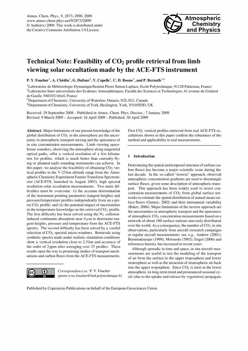
Fig. 1. Atmospheric N2 continuum (and associated N2 quadrupole
lines) transmittance in the 2400–2600 cm spectral range for 9 geo-
metric tangent heights from 5 km to 25 km from 4A/OP-limb RTM.
3 Spectral micro-window selection
3.1 Spectral micro-window pre selection: a sensitivity
analysis
To be selected and finally included in the measurement vec-
tor, a spectral micro-window must satisfy the obvious criteria
of high sensitivity to the target variables (here the pointing
parameters or CO2) and low sensitivity to non target vari-
ables. Investigations have to be carried out to analyze the
quality of the spectral fit in order to minimize systematic con-
tributions to the final error budget.
3.1.1 Pointing parameters and the N2 continuum ab-
sorption
As explained in Sect. 2, micro-windows are selected in the
N2 collision-induced absorption continuum near 4.0µmto fit
tangent heights and pT profiles in the 5–25 km altitude range.
N2 continuum absorption is significant for large optical pathsobtained in the limb viewing geometry. 4A/OP-limb RTM
uses an empirical model (Lafferty, 1996) determined from
experimental data, which includes N2-N2 and N2-O2 colli-
sions and covers the 190–300 K temperature range. Mea-
surements cover the range 2125 cm (4.7µm) to 2600 cm
(3.8µm) with a spectral resolution of 0.25 cm−1. N2 contin-
uum absorption becomes too weak to be used above 25 km
and most of the band becomes saturated below 5 km; the
atmospheric transmittance dynamic range is large in the 5–
25 km altitude range as seen in Fig. 1. This spectral region
0
0.1
0.2
0.3
0.4
0.5
0.6
0.7
0.8
0.9
1
2460 2480 2500 2520 2540
T r a n s m i s s i o n
Wavenumber (cm -1)
Geometric tangent height 8.65 km
N2N2OCO2
all
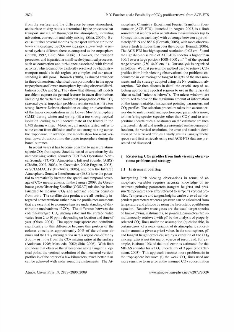
Fig. 2. Atmospheric transmittance in the 2450–2550 cm spec-
tral range at 8.65 km (geometric tangent height) from 4A/OP-limb
RTM. The N2 continuum (and associated N2 quadrupole lines) is
represented in red. CO2 and N2O absorptions are represented in
blue and green, respectively. Total absorption is in grey.
also contains absorption from N2O and CO2 lines. The far
wing contributions from these molecules, which are difficult
to model, may affect the baseline level in the vicinity of the
N2 continuum (see Figs. 2 and 3), thereby complicating the
analysis. For wavenumbers below 2385 cm the spectrum is
saturated up to 25 km due to CO2 far wing absorption and theeffect of this contribution on the N2 baseline remains signifi-
cant up to 2500 cm for the lowest altitudes and up to 2450 cm
at 20 km. The contribution from N2O line wings is impor-
tant for the lowest altitudes from 2400 cm to 2495 cm and
from 2515 cm to 2600cm but the N2O and CO2 impact on
the baseline rapidly decreases with increasing tangent height
(see Fig. 3 for a geometric tangent height of 15.9 km). The
geometric tangent height is the tangent altitude of the opti-
cal path without refraction. This geometric optical path is
tangent to the true optical path (with refraction) at the satel-
lite position. So, geometric tangent heights are always higher
than true tangent heights. Figure 2 shows that at 8.65 km geo-metric tangent height (corresponding to a true tangent height
around 7.7 km), CO2 and N2O contributions to the N2 ab-
sorption are only negligible in a small spectral region around
2500 cm−1, whereas at 15.90 km, Fig. 3 shows that a larger
spectral region, from 2480 to 2520 cm−1, is available. In
summary, the spectral ranges employed for pointing param-
eter retrieval using the N2 continuum are as follows: 2495–
2505 cm in the 5–10 km altitude range, 2490–2520 cm in the
10–15 km altitude range, 2480–2505 cm and around 2461 cm
in the 15–25 km altitude range.
Atmos. Chem. Phys., 9, 2873–2890, 2009 www.atmos-chem-phys.net/9/2873/2009/
8/2/2019 P. Y. Foucher et al- Technical Note: Feasibility of CO2 profile retrieval from limb viewing solar occultation made by t…
http://slidepdf.com/reader/full/p-y-foucher-et-al-technical-note-feasibility-of-co2-profile-retrieval-from 5/18
P. Y. Foucher et al.: Feasibility of CO2 profile retrieval from ACE-FTS 2877
0
0.2
0.4
0.6
0.8
1
2460 2480 2500 2520 2540
T r a n s m i s s i o n
Wavenumber (cm -1)
Geometric tangent height 15.94 km
N2CO2N2O
all
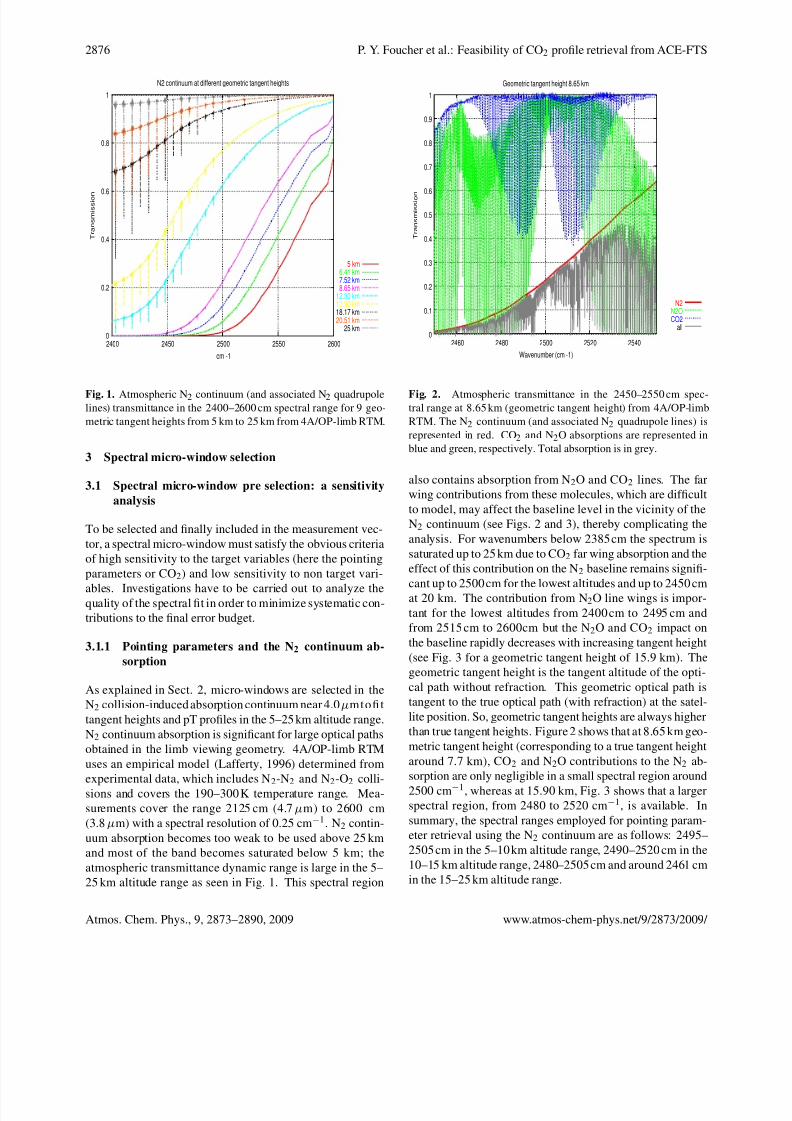
Fig. 3. Atmospheric transmittance in the 2450–2550 cm spec-
tral range at 15.9 km (geometric tangent height) from 4A/OP-limb
RTM. The N2 continuum (and associated N2 quadrupole lines) is
represented in red. CO2 and N2O absorptions are represented in
blue and green, respectively. Total absorption is in grey.
The pure N2 collision-induced absorption temperature de-
pendence varies with wavenumber (Lafferty, 1996). Below
2450 cm−1, the absorption coefficient decreases with tem-
perature, while the reverse is true for wavenumbers above
2450 cm−1; however the sensitivity to variations in tangentheight is relatively constant throughout the continuum. To re-
trieve temperature and tangent height simultaneously above
12 km (see part 2.1), it is necessary to choose at least two
different N2 spectral micro-windows having different sensi-
tivities to temperature, i.e., micro-windows around 2450 cm
(or below) and micro-windows around 2500 cm−1. How-
ever, in the 2450 cm spectral range, absorption is very high
below 10 km and is influenced by the N2O and CO2 line far
wings. In this paper we therefore focus mainly on tangent
height retrievals although the results of a simultaneous fit are
presented in part 5.
3.1.2 CO2 concentrations: an analysis of CO2 line sen-
sitivity
The selection of CO2 spectral micro-windows for both con-
centration and temperature retrievals is based on the anal-
ysis of 4A/OP-limb RTM simulated transmittances and Ja-
cobians. In a first step, CO2 lines with concentration Jaco-
bians peaking within the tangent altitude range considered
are selected. In a second step, CO2 lines overlapped by other
species are rejected on the basis of the relative importance
of the CO2 Jacobian and the Jacobians of the other species.
In a third step, only the CO2 lines with a small lower state
energy E are selected to minimize the line intensity depen-
dence on temperature. In fact, it may be shown that for a
micro-window corresponding to a CO2 line with a low value
of the lower state energy E, there exists a tangent height at
which the temperature Jacobian is almost equal to zero (Park,
1997) and the sign of the temperature Jacobian is positiveabove this critical altitude and negative below.
Altogether, about 80 CO2 micro-windows were pre-
selected from five different spectral domains as shown in Ta-
ble 3.1.2 (column 1: number of micro-windows; column 2:
spectral domain and isotopologue). In this table they are clas-
sified according to the altitude range in which they are suit-
able for determining the CO2 profile (column 3). Column 4
gives the average value of E for the lines selected in each
spectral domain. These values are much smaller than those
corresponding to micro-windows traditionally selected for
temperature retrieval when the target variable is not CO2 (see
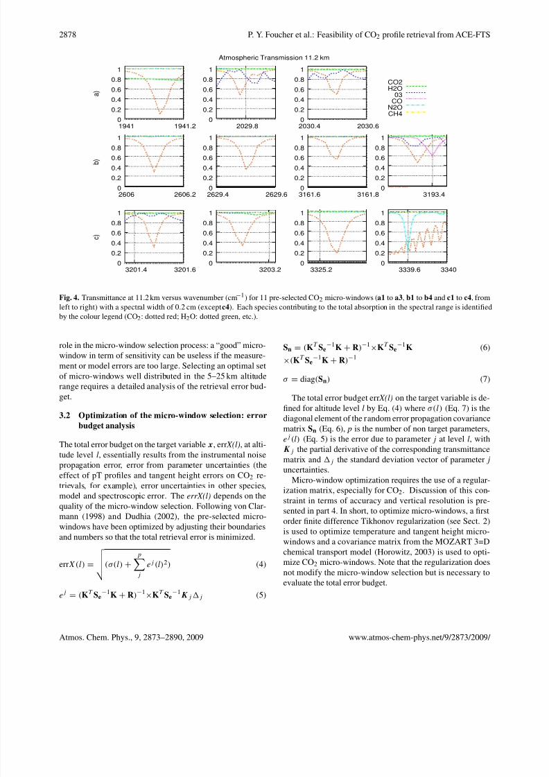
column 5). Figures 4 and 5 show examples of pre-selectedCO2 micro-windows transmittances (Fig. 4) and sensitivities
(Fig. 5), for each contributing species, versus wavenumber at
a tangent height of 11.2 km. In Fig. 4, different situations
are seen: (i) relatively clean CO2 windows (b1, b2, b3, c2
and c3); (ii) windows with modest contributions from other
species (O3 in a3 and c1); windows with more pronounced
signatures from other species (H2O in a1, O3 in a2, CO in
b4, and N2O in c4). The impact of other species, such as
CH4, has also been tested (although no results are presented
here). Figure 5 shows transmittance Jacobians for the same
species and for the same CO2 micro-windows. In this fig-
ure the temperature Jacobians are also plotted (black dashed
line) which display different behaviours: positive sensitiv-
ity for a1, b1, and c3; negative sensitivity for a2, a3, b3, c1
and c2; sensitivity changing sign within the spectral inter-
val for b4 and c4. Almost zero sensitivity is observed for
b2. The expected presence of opposite temperature Jaco-
bian signs, between 2030 cm and 2606 cm for example, is
a very interesting point. Indeed, if two CO2 lines with op-
posite temperature Jacobians for the same altitude range are
used for CO2 retrieval, the impact of temperature uncertain-
ties on the retrieval in this altitude range is reduced (see part
3.2 on micro-windows optimization). When a micro-window
is nearly free of absorption by other species, an easy method
to select (or reject) the micro-window is to look at the ra-tio between its sensitivity to temperature to its sensitivity to
CO2. The presence of an interfering species may be seen as
a problem in terms of the error budget. However, this inter-
ference can lead to the temperature sensitivity changing sign
within the micro-window (as in b4, for example) which may
result in a less significant temperature sensitivity than for a
cleaner micro-window with a more uniform (positive or neg-
ative) temperature sensitivity.
The instrumental noise, as well as the ability of the RTM
to properly model the transmittance, also plays an important
www.atmos-chem-phys.net/9/2873/2009/ Atmos. Chem. Phys., 9, 2873–2890, 2009
8/2/2019 P. Y. Foucher et al- Technical Note: Feasibility of CO2 profile retrieval from limb viewing solar occultation made by t…
http://slidepdf.com/reader/full/p-y-foucher-et-al-technical-note-feasibility-of-co2-profile-retrieval-from 6/18
2878 P. Y. Foucher et al.: Feasibility of CO2 profile retrieval from ACE-FTS
Atmospheric Transmission 11.2 km
0
0.2
0.4
0.6
0.8
1
1941 1941.2
a )
0
0.2
0.4
0.6
0.8
1
2029.8
0
0.2
0.4
0.6
0.8
1
2030.4 2030.6
CO2H2O
03CO
N2OCH4
0
0.2
0.4
0.6
0.8
1
2606 2606.2
b )
0
0.2
0.4
0.6
0.8
1
2629.4 2629.60
0.2
0.4
0.6
0.8
1
3161.6 3161.80
0.2
0.4
0.6
0.8
1
3193.4
00.2
0.4
0.6
0.8
1
3201.4 3201.6
c )
00.2
0.4
0.6
0.8
1
3203.20
0.2
0.4
0.6
0.8
1
3325.20
0.2
0.4
0.6
0.8
1
3339.6 3340
Fig. 4. Transmittance at 11.2 km versus wavenumber (cm−1) for 11 pre-selected CO2 micro-windows (a1 to a3, b1 to b4 and c1 to c4, from
left to right) with a spectral width of 0.2 cm (except c4). Each species contributing to the total absorption in the spectral range is identified
by the colour legend (CO2: dotted red; H2O: dotted green, etc.).
role in the micro-window selection process: a “good” micro-
window in term of sensitivity can be useless if the measure-
ment or model errors are too large. Selecting an optimal set
of micro-windows well distributed in the 5–25 km altitude
range requires a detailed analysis of the retrieval error bud-
get.
3.2 Optimization of the micro-window selection: error
budget analysis
The total error budget on the target variable x, err X(l), at alti-
tude level l, essentially results from the instrumental noise
propagation error, error from parameter uncertainties (the
effect of pT profiles and tangent height errors on CO2 re-
trievals, for example), error uncertainties in other species,
model and spectroscopic error. The errX(l) depends on the
quality of the micro-window selection. Following von Clar-mann (1998) and Dudhia (2002), the pre-selected micro-
windows have been optimized by adjusting their boundaries
and numbers so that the total retrieval error is minimized.
errX(l) =
(σ(l) +
pj
ej (l)2) (4)
ej = (KT Se−1K + R)−1
×KT Se−1Kjj (5)
Sn = (KT Se−1K + R)−1
×KT Se−1K (6)
×(KT Se−1K + R)−1
σ = diag(Sn) (7)
The total error budget err X(l) on the target variable is de-
fined for altitude level l by Eq. (4) where σ(l) (Eq. 7) is the
diagonal element of the random error propagation covariance
matrix Sn (Eq. 6), p is the number of non target parameters,
ej (l) (Eq. 5) is the error due to parameter j at level l, with
Kj the partial derivative of the corresponding transmittance
matrix and j the standard deviation vector of parameter j
uncertainties.
Micro-window optimization requires the use of a regular-
ization matrix, especially for CO2. Discussion of this con-
straint in terms of accuracy and vertical resolution is pre-
sented in part 4. In short, to optimize micro-windows, a firstorder finite difference Tikhonov regularization (see Sect. 2)
is used to optimize temperature and tangent height micro-
windows and a covariance matrix from the MOZART 3=D
chemical transport model (Horowitz, 2003) is used to opti-
mize CO2 micro-windows. Note that the regularization does
not modify the micro-window selection but is necessary to
evaluate the total error budget.
Atmos. Chem. Phys., 9, 2873–2890, 2009 www.atmos-chem-phys.net/9/2873/2009/
8/2/2019 P. Y. Foucher et al- Technical Note: Feasibility of CO2 profile retrieval from limb viewing solar occultation made by t…
http://slidepdf.com/reader/full/p-y-foucher-et-al-technical-note-feasibility-of-co2-profile-retrieval-from 7/18
P. Y. Foucher et al.: Feasibility of CO2 profile retrieval from ACE-FTS 2879
Atmospheric Transmission Sensitivities 11.2 km
-0.006-0.005-0.004-0.003-0.002-0.001
00.001
1941 1941.2
a )
-0.006-0.005-0.004-0.003-0.002-0.001
00.001
2029.8
-0.006-0.005-0.004-0.003-0.002-0.001
00.001
2030.4 2030.6
CO2H2O
03CO
N2OT
-0.006-0.005-0.004-0.003-0.002-0.001
00.001
2606 2606.2
b )
-0.006-0.005-0.004-0.003-0.002-0.001
00.001
2629.4 2629.6-0.006-0.005-0.004-0.003-0.002-0.001
00.001
3161.6 3161.8-0.006-0.005-0.004-0.003-0.002-0.001
00.001
3193.4
-0.006-0.005
-0.004-0.003-0.002-0.001
00.001
3201.4 3201.6
c )
-0.006-0.005
-0.004-0.003-0.002-0.001
00.001
3203.2-0.006-0.005
-0.004-0.003-0.002-0.001
00.001
3325.2-0.006-0.005
-0.004-0.003-0.002-0.001
00.001
3339.6 3340
Fig. 5. Transmittance Jacobians at 11.2 km versus wavenumber (cm−1) for 11 pre-selected CO2 micro-windows (a1 to a3, b1 to b4 and c1
to c4, from left to right) and for each species contributing to the total absorption in the spectral range, identified by the colour legend (CO2:
dotted red; H2O: dotted green, etc.). Black dashed lines are for the temperature Jacobians. Species Jacobians other than CO2 are for a 2%
variation in their concentration; CO2 Jacobians are for a variation of 5 ppm of its concentration; temperature Jacobians are for a variation of
1 K.
Table 1. CO2 microwindow families.
number of mw CO2 spectral domain (cm−1
) altitude rangea
(km) E
(cm−1
)b
E
(cm−1
)c
12 1920–1955/ 12C16O2 9–25 150.2 512.2
13 2010–2030/ 13C16O2 7–20 162.8
32 2600–2635/ 18OC16O 5–15 61.6
9 3150–3205/ 12C16O2 5–25 182.6
16 3315–3355/ 12C16O2 5–25 154.6 777.4
a not all microwindows of each family are used for the same altitude rangeb mw used for CO2 retrievalc mw used for T retrieval
3.2.1 Optimized N2 continuum micro-windows
For each spectral range available (see Sect. 3.1.1), optimum
micro-windows are selected to minimize the CO2 and N2O
far wing contribution to the N2 baseline continuum absorp-
tion and the retrieval error in general. Starting from a min-
imal width of 1 cm for an optimized micro-window, the to-
tal retrieval error is estimated as a function of the increas-
ing width of the window. The random noise error, errors
due to 5% percent changes in CO2 and N2O concentrations,
and model errors due to CO2 and N2O far wing contribu-
tions and N2 continuum, estimated on the basis of compar-
isons with ACE-FTS measurements and experimental mea-
surements (Lafferty, 1996), are taken into account in this
analysis. The random noise variance used here is taken as
twice the instrument noise variance to account for random
errors from computation. Figure 6 shows the variation of
the total error and of error components (random noise, CO 2,
N2O, model) as a function of the width of the micro-window
for the spectral range around 2500 cm−1. These errors have
www.atmos-chem-phys.net/9/2873/2009/ Atmos. Chem. Phys., 9, 2873–2890, 2009
8/2/2019 P. Y. Foucher et al- Technical Note: Feasibility of CO2 profile retrieval from limb viewing solar occultation made by t…
http://slidepdf.com/reader/full/p-y-foucher-et-al-technical-note-feasibility-of-co2-profile-retrieval-from 8/18
2880 P. Y. Foucher et al.: Feasibility of CO2 profile retrieval from ACE-FTS
Table 2. Altitude retrieval error of selected N2 microwindows.
N2 spectral range (cm−1) altitude range (km) error (km)
2461.2–2462.8 15–20 70.10−3
2504–2507 10–15 75.10−3
2491.1–2493.1 12–17 65.10−3
2498.5–2501.5 10–17 50.10
−3
2498–2502 5–10 40.10−3
been averaged for tangent heights between 5 and 10 km. The
initial micro-window width is 1 cm (50 spectral points) and
its central wavenumber is 2500. 7 cm−1, which corresponds
to the centre of the CO2 band (see Figs. 2 and 3). Then,
step by step, 2 symmetric spectral points are added and the
tangent height retrieval error is again estimated. From 1 cm
to 9 cm width, the noise propagation error decreases from
25 m to 9 m, the model error increases from 35 m to 42 m,
the error due to uncertainties in CO2
and N2
O concentra-
tion remains less than 5 m. The total error reaches its min-
imum value (about 40 m) at 3.5 cm width and remains ap-
proximately constant for larger widths. Similar results are
obtained for the same spectral range for the 10–15 km alti-
tude range (not shown). The total error comes to about 50 m;
model error significantly increases with the width (due to
CO2 far wing model error as the N2 continuum model er-
ror is quite constant in this spectral region); retrieval errors
due to N2O and CO2 concentration uncertainties remain low
(less than 5 m). For this altitude range, in the spectral in-
terval 2495–2505 cm−1, the optimal micro-window width is
3 cm−1. Results for the same altitude range in other spec-
tral intervals, 2490–2495 cm and 2505–2520 cm−1, are alsointeresting. Optimized micro-windows resulting from this
spectral analysis are presented in Table 2 for tangent height
retrieval in the range 5–25 km.
3.2.2 Optimized set of CO2 line micro-windows
In the case of CO2, many micro-windows may be consid-
ered for retrieving its concentration at a given altitude. Op-
timization of the set of pre-selected micro-windows is based
on the evaluation of component and total errors due to noise
propagation, temperature uncertainties, and, eventually, in-
terfering species. The random noise introduced accounts forinstrumental noise and CO2 random spectroscopic parame-
ters error. Resulting from comparisons between observations
and model simulations, the transmittance model random er-
ror for CO2 has been taken equal to 0.5×10⁻² (i.e., twice
as larger as instrumental random noise in the center of the
band). Micro-window selection follows two main steps: (i)
optimization of the width of each micro-window, (ii) creation
of an optimum set of micro-windows.
For each pre-selected micro-window we first evaluate the
impact of its spectral width on the retrieval error. Fig. 7a to
Tangent height retrieval errors for the 5-10km altitude rangearound 2500 cm-1
Random noise
N2O
CO2
model
Total
E r r o r ( k m )
Width (cm-1)
Fig. 6. Tangent height retrieval errors (in km) for the 5–10 km
altitude range as a function of the micro-window width (cm−1).
Micro-window centred at 2500.7 cm−1. Red: random noise er-
ror; blue and green: errors due to uncertainties on CO2 and N2O,
respectively; pink: model error due to N2 continuum uncertainty,
CO2 and N2O far wing contributions; blue: total error.
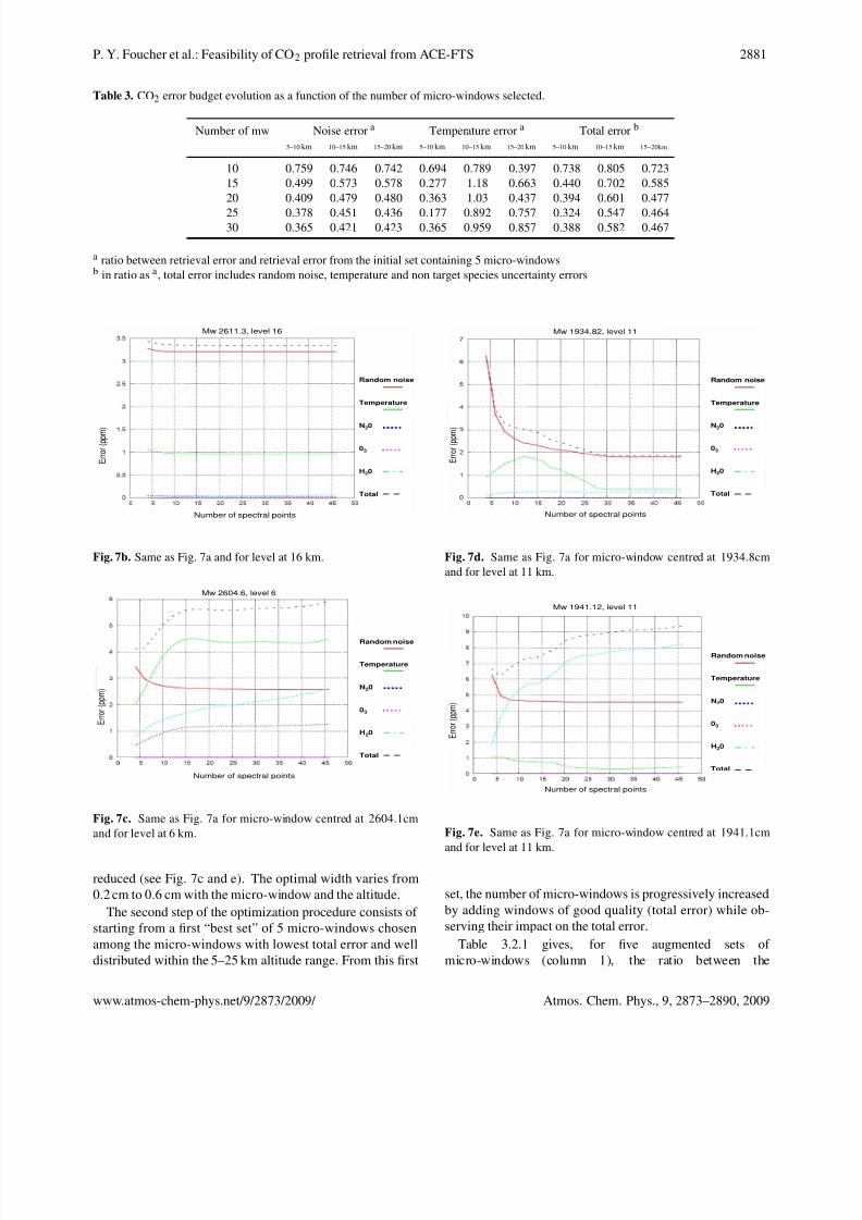
Mw 2611.3, level 6
E r r o r ( p p m )
Number of spectral points
Random noise
Temperature
N20
03
H20
Total
Fig. 7a. CO2 retrieval errors (in ppm) for level at 6 km as a
function of the micro-window number of spectral points (spectral
step=0.02 cm−1). Micro-window centred at 2611.3 cm−1. Red:
random noise error; blue, pink and pale blue: errors due to uncer-
tainties on N2O, O3 and H2O, respectively; dark: total error.
7e show retrieval error evolution with micro-window width
for 4 different micro-windows at different tangent heights.
Usually there is a significant decrease in noise propagationerror with the width as seen in Fig. 7a, however interfering
species error and temperature error evolution with width is
not monotonic (see Fig. 7d) and depends on the altitude (see
Fig. 7a and Fig. 7b). The optimal width of a micro-window
increases when altitude decreases in order to reduce as much
as possible noise error propagation. An interesting point is
that interfering species can sometimes make temperature er-
ror decrease (see Fig. 7d). Finally, for each altitude, pre-
selected width-optimized micro-windows are ranked accord-
ing to their total error or rejected if the total error cannot be
Atmos. Chem. Phys., 9, 2873–2890, 2009 www.atmos-chem-phys.net/9/2873/2009/
8/2/2019 P. Y. Foucher et al- Technical Note: Feasibility of CO2 profile retrieval from limb viewing solar occultation made by t…
http://slidepdf.com/reader/full/p-y-foucher-et-al-technical-note-feasibility-of-co2-profile-retrieval-from 9/18
P. Y. Foucher et al.: Feasibility of CO2 profile retrieval from ACE-FTS 2881
Table 3. CO2 error budget evolution as a function of the number of micro-windows selected.
Number of mw Noise error a Temperature error a Total error b
5–10 km 10–15 km 15–20 km 5–10 km 10–15 km 15–20 km 5–10 km 10–15 km 15–20km
10 0.759 0.746 0.742 0.694 0.789 0.397 0.738 0.805 0.723
15 0.499 0.573 0.578 0.277 1.18 0.663 0.440 0.702 0.585
20 0.409 0.479 0.480 0.363 1.03 0.437 0.394 0.601 0.47725 0.378 0.451 0.436 0.177 0.892 0.757 0.324 0.547 0.464
30 0.365 0.421 0.423 0.365 0.959 0.857 0.388 0.582 0.467
a ratio between retrieval error and retrieval error from the initial set containing 5 micro-windowsb in ratio as a, total error includes random noise, temperature and non target species uncertainty errors
Random noise
Temperature
N20
03
H20
Total
Mw 2611.3, level 16
E r r o r ( p p m )
Number of spectral points
Fig. 7b. Same as Fig. 7a and for level at 16 km.
Random noise
Temperature
N20
03
H20
Total
Mw 2604.6, level 6
E r r o r ( p p m )
Number of spectral points
Fig. 7c. Same as Fig. 7a for micro-window centred at 2604.1cm
and for level at 6 km.
reduced (see Fig. 7c and e). The optimal width varies from
0.2 cm to 0.6 cm with the micro-window and the altitude.
The second step of the optimization procedure consists of
starting from a first “best set” of 5 micro-windows chosen
among the micro-windows with lowest total error and well
distributed within the 5–25 km altitude range. From this first
Random noise
Temperature
N20
03
H20
Total
Mw 1934.82, level 11
E r r o r ( p p m )
Number of spectral points
Fig. 7d. Same as Fig. 7a for micro-window centred at 1934.8cm
and for level at 11 km.
Random noise
Temperature
N20
03
H20
Total
Mw 1941.12, level 11
E r r o r ( p p m )
Number of spectral points
Fig. 7e. Same as Fig. 7a for micro-window centred at 1941.1cm
and for level at 11 km.
set, the number of micro-windows is progressively increased
by adding windows of good quality (total error) while ob-
serving their impact on the total error.
Table 3.2.1 gives, for five augmented sets of
micro-windows (column 1), the ratio between the
www.atmos-chem-phys.net/9/2873/2009/ Atmos. Chem. Phys., 9, 2873–2890, 2009
8/2/2019 P. Y. Foucher et al- Technical Note: Feasibility of CO2 profile retrieval from limb viewing solar occultation made by t…
http://slidepdf.com/reader/full/p-y-foucher-et-al-technical-note-feasibility-of-co2-profile-retrieval-from 10/18
2882 P. Y. Foucher et al.: Feasibility of CO2 profile retrieval from ACE-FTS
corresponding total error and that obtained with the
original 5-micro-window set. Regarding the random noise
error (columns 2–4), the retrieval error decreases when
the number of micro-windows increases at each altitude
range. A limit is reached for the set with 30 micro-windows.
Temperature error (columns 5–7) behaviour varies with the
altitude range: (i) in the 5–10 km altitude range the error
decreases up to the 15 micro-windows set and then fluctuateswith a minimum for the 25 micro-windows set, this being
due to the fact that, for this altitude range, the temperature
sensitivity sign frequently changes from one micro-window
to another, leading to error compensation; (ii) in the 10–
15 km altitude range the temperature sensitivity sign is more
stable with slightly larger values for the augmented sets
than for the initial 5-micro-window set: this set has been
optimized to reduce temperature error in this altitude range;
(iii) the 15–20 km altitude range error values are lower than
for the initial 5-micro-window set with some important
fluctuations with a minimum for the 10-micro-window
set and a maximum for the 30-micro-window set. Thetotal retrieval error (column 8–10) includes random noise,
temperature and non target species uncertainty errors. It
decreases when the number of micro-windows increases
and validates this second step of the optimization process.
However, from the 25 to the 30 micro-window set, the total
error slightly increases at each altitude range: adding more
pre selected micro-windows no longer improves the retrieval
performance. Indeed, the noise error reaches its limit and
the temperature error begins to increase significantly at each
altitude range. The optimal 25-micro-window set is used in
the following analysis.
4 Retrieval error analysis: accuracy and vertical reso-
lution
The choice of an appropriate regularization matrix R (see
Sect. 2.2), which may either smooth the retrieval or constrain
its final state towards an a priori known state, has a direct im-
pact on the retrieval error as it governs the balance between
the information brought by the signal and that brought by the
constraint.
4.1 Choice of the regularization matrix R
As stated in Sect. 2, one of the best choices for R is the in-
verse a priori CO2 covariance matrix Sa, provided it is known
accurately enough. Here, Sa and associated a priori profiles
xa have been calculated by the MOZART-CTM version 2
(Horowitz, 2003). These a priori matrices and profiles have
been estimated for each season, and for five latitude bands
(from −90◦ to +90◦ by 30◦) covering all longitudes. Diag-
onal elements of Sa represent the expected variance of the
CO2 mixing ratio at each altitude and non diagonal elements
represent the vertical correlation between CO2 mixing ratios
Table 4. CO2 retrieval degrees of freedom for the 5–20 km altitude
range as a function of α.
df α
8 2.165×10⁻³
9 8.50×10⁻⁴
10 4.05×10⁻⁴
at different altitudes. However, the impact of such a con-
straint on the retrieval is quite strong due to the presence of
significant noise and the regularisation matrix R is often as-
sumed to be equal to the product αSa−1, where α is a scalar
less than unity. The optimized value of α for the retrieval
must ensure a good vertical resolution and a good accuracy.
In the case of tangent height retrievals, we use a first order
Tikhonov regularization as no covariance a priori data are
available.
4.2 Averaging kernel
The instrument has an input aperture of 1.25 mrad, which
subtends an altitude range of 3–4km at the tangent point.
However, the altitude spacing between two sequential mea-
surements in the 5–25 km range varies from about 3 km to
less than 1 km and suggests that the effective vertical reso-
lution of the ACE-FTS can be better than the field-of-view
limit (Hegglin, 2008) if, for example, some deconvolution
technique is used. For the purposes of this study, we will
define the vertical resolution using the averaging kernel ma-
trix, A, and our analysis does not explicitly include the effect
of the finite field-of-view of the instrument. To estimate thevertical resolution of the retrieval we use the averaging ker-
nel matrix A written as:
A = (KT Se−1K + R)−1
×KT Se−1K =
∂x∂x
(8)
df = tr(A) (9)
A is the averaging kernel matrix,x is the retrieved profile
and x is the input profile: the kth element of row j of the aver-
aging kernel matrix represents the sensitivity of level j of the
retrieved profile
x to a 1 ppm change in the CO2 mixing ratio
of level k of the input profile x. The trace of the averaging
kernel matrix, df (Eq. 9), is equal to the degrees of freedom
of the retrieval. When no constraint is applied, the averaging
kernel is the identity matrix and the degrees of freedom of
the retrieval is equal to the number of grid levels: the vertical
resolution would here be equal to 1 km. Assuming a ver-
tical resolution of about 2 km, corresponding to an average
number of nine ACE-FTS measurements in the 5–25 km alti-
tude range, the expected degrees of freedom for the retrieval
comes to 9 which corresponds to an initial value of alpha of
the order of 8.5×10⁻⁴.
Atmos. Chem. Phys., 9, 2873–2890, 2009 www.atmos-chem-phys.net/9/2873/2009/
8/2/2019 P. Y. Foucher et al- Technical Note: Feasibility of CO2 profile retrieval from limb viewing solar occultation made by t…
http://slidepdf.com/reader/full/p-y-foucher-et-al-technical-note-feasibility-of-co2-profile-retrieval-from 11/18
P. Y. Foucher et al.: Feasibility of CO2 profile retrieval from ACE-FTS 2883
4
5
6
7
8
9
10
11
12
13
14
15
16
17
18
19
20
21
22
23
24
25
-0.2 -0.1 0 0.1 0.2 0.3 0.4 0.5 0.6 0.7 0.8 0.9 1
a l t i t u d e ( k m )
CO2 Avera in kerne l m/ m)
lev 5lev 6lev 7lev 8lev 9
lev 10lev 11lev 12lev 13lev 14lev 15lev 16lev 17lev 18lev 19lev 20lev 21lev 22lev 23lev 24
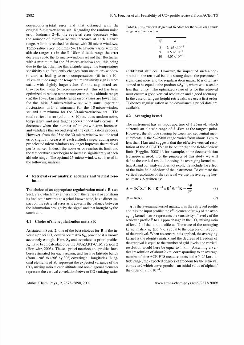
Fig. 8. Averaging kernel (row of A) for a retrieval degree of freedom
equal to 9. Each curve labelled l on the right color legend represents
the sensitivity, given in abscissa in ppm of CO2, of the retrieval
at level l to a 1 ppm change made at the altitude (in km) given in
ordinate. Each row of A corresponds to a retrieval level and to a
coloured curve as indicated by the colour legend on the right. For
example, the red curve labelled “lev 15” in this legend represents
the sensitivity, given in abscissa in ppm of CO2, of the retrieval at
level 15 (15 km altitude) to a 1 ppm change made at altitude given
in ordinate.
4.3 Vertical resolution
Figure 8 illustrates the averaging kernel for a degree of free-
dom of 9. For this example, level 15 averaging kernel values
at altitude 15 km are slightly larger than 0.6. The maximum
of level l averaging kernel generally occurs at altitude l and
the vertical resolution corresponds to the half-width of the
sensitivity distribution. For example, the vertical resolution
of level 15 retrieval is close to 2 km. Figure 8 also shows that
the peaks of the sensitivity distributions do not always cor-respond to the altitude at which the 1 ppm change has been
made. For example, “lev 8”, “lev10” and “lev 12” curves
peak, respectively, at altitudes 7 km, 9 km and 11 km and
their peak values are smaller than those of “lev 7”, “lev 9”
and “lev 11” peaks and their associated vertical resolution is
worse (around 3 km instead 2 km). This means that retrievals
are (respectively) more sensitive to changes at altitudes 7 km,
9 km and 11 km than at 8 km, 10 km and 12 km. This differ-
ence simply comes from the fact that the retrieval grid is finer
than the measurement grid. Measurement tangent heights
(measurement grid) are closer, in this case, to the retrieval
grid at altitudes 7 km, 9 km and 11 km than at 8 km, 10 km
and 12 km altitudes. As expected, the retrievals are more sen-
sitive near the observed tangent heights. Peak values are al-
ways larger than 0.5 (except in the 20–25 km altitude range),
which confirms that the retrieval has been made using in-
formation primarily from the measurements rather than from
the regularization (Koner, 2008) and that the retrieval gridof 1 km is adapted to the measurements. The decrease in
the vertical resolution seen in the 20–25 km altitude range is
due to a lack of CO2 lines sufficiently sensitive to CO2 con-
centration and sufficiently insensitive to temperature. As a
consequence, averaging kernel peak values decrease. Above
20 km, information preferentially comes from the a priori
vector.
4.4 Impact of the constraint on the retrieval error
To quantify the impact of the constraint on the retrieval error
and to determine the best α value, we carried out retrievals
on synthetic spectra taking into account instrumental noise
and an uncertainty in atmospheric temperature with no bias
and a standard deviation of 1 K (random noise). A set of 25
synthetic occultations were generated using a common “true”
CO2 profile and different patterns for the random noise. CO2
profiles are retrieved from each of these synthetic occulta-
tions. We performed the retrievals using different values of
α around the initial pre selected value corresponding to 9 de-
grees of freedom. The choice of an optimized α is based on
the calculation of the standard deviation between the mean
retrieved profile and the true profile averaged over the alti-
tude range 5–25 km (“accuracy”) and the standard deviation
of the sample of 25 retrieved profiles (again 5–25 km aver-age; “precision”). First, an important difference is seen be-
tween the “accuracy” and the “precision” results. This is due
to spurious oscillations of the retrieved profiles around the
true profile: they mostly compensate each other in the “ac-
curacy” result whereas they clearly appear in the “precision”
result for the lowest value of α. For higher values of α, the
mean retrieved profile tends to a priori with no more spuri-
ous oscillations, the mean total error increases whereas the
standard deviation decreases. Results of this analysis lead
to degrees of freedom between 8 and 9, corresponding to a
value of alpha of 0.001 (we have verified that, applied to real
occultations, this value of α actually minimizes the measure-
ment part of the residual (first term of the right hand side of
Eq. 1).
www.atmos-chem-phys.net/9/2873/2009/ Atmos. Chem. Phys., 9, 2873–2890, 2009
8/2/2019 P. Y. Foucher et al- Technical Note: Feasibility of CO2 profile retrieval from limb viewing solar occultation made by t…
http://slidepdf.com/reader/full/p-y-foucher-et-al-technical-note-feasibility-of-co2-profile-retrieval-from 12/18
2884 P. Y. Foucher et al.: Feasibility of CO2 profile retrieval from ACE-FTS
6
8
10
12
14
16
18
20
-0.5 - 0.4 - 0.3 - 0.2 - 0.1 0 0 .1 0 .2 0.3 0 .4 0.5
G e o m e t r i c
A l t i t u d e
(
k m )
Relative error (km)
Initial tangent height errors
6
8
10
12
14
16
18
20
-0.09 -0.06 -0.03 0 0.03 0.06 0.09
Relative error (km)
Retrieved tangent height errors
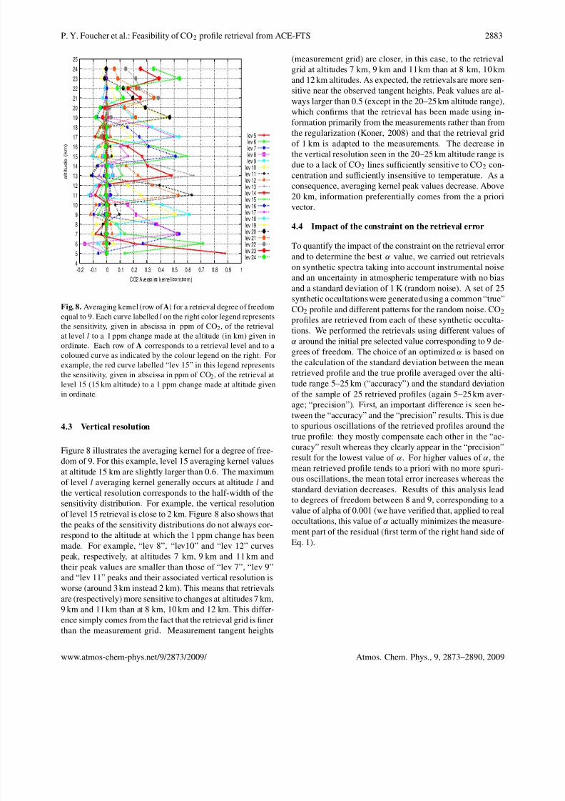
Fig. 9a. Single tangent height retrieval from N2 continuum spec-
tral windows in the 5–20 km altitude range using ACE level 2.2
temperature profile: results from 25 synthetic tests. Mean initial
tangent height statistics (left): bias in dotted dark line and standard
deviation (dark error bars). Mean retrieved tangent height statis-
tics (right): bias in dotted red line and standard deviation (red error
bars).
6
8
10
12
14
16
18
20
-0. 5 - 0. 4 - 0. 3 - 0.2 - 0. 1 0 0 .1 0 .2 0 .3 0. 4 0 .5
G e o m e t r i c
A l t i t u d e
( k m )
Relative error (km)
Initial tangent height errors
6
8
10
12
14
16
18
20
-0.09 -0.06 -0.03 0 0.03 0.06 0.09
Relative error (km)
Retrieved tangent height errors
Fig. 9b. The same as Fig. 9a with 1 K bias and 1 K random noise
added to the ACE level 2.2 temperature profile.
6
8
10
12
14
16
18
20
-0.5 - 0.4 - 0.3 - 0.2 - 0.1 0 0 .1 0 .2 0.3 0 .4 0 .5
G e o m e t r i c
A l t i t
u d e
( k m )
Relative error (km)
Initial tangent height errors
6
8
10
12
14
16
18
20
-0.09 -0.06 -0.03 0 0.03 0.06 0.09
Relative error (km)
Retrieved tangent height errors
Fig. 9c. The same as Fig. 9b with simultaneous tangent height and
temperature retrieval.
5 Application to real data, results and discussion
5.1 Tangent height
5.1.1 Discussion of synthetic tests
Following the procedure described in Sect. 3, tangent height
N2-retrievals on synthetic occultations have been carried out
taking into account various options for the instrumental noise
and an initial guess tangent height standard deviation of
0.3 km with no bias. Figure 9a (left) shows initial guess
statistics (mean: dotted line; standard deviation: solid bars)
over the 25 cases used in Sect. 4.4). Figure 9a (right), which
assumes knowledge of the temperature, here from ACE v2.2
data, shows the mean tangent height retrieval error statistics:
the standard deviation error (solid bars) is less than 20 m with
almost no bias. For these synthetic tests, no model errors
were introduced; consequently, an error of about 50 m (see
Table 2) due to model uncertainties must be added to this
result. Figure 9b shows similar results when knowledge of
the temperature profile is not assumed: an uncertainty with
a 1 K random error and a 1 K bias is introduced. On Fig. 9b
(right), we see resulting tangent height biases varying withaltitude: −10m below 8 km, +30 m between 8 and 14km and
+70 m above. Standard deviations are larger, up to 100 m at
14 or 16 km. As mentioned in Sect. 3.1.1, simultaneous tan-
gent height and temperature retrieval in principle requires the
use of two different N2 micro-windows to ensure stability.
However, using the set of micro-windows of Table 2, Fig. 9c
shows results corresponding to the same case as Fig. 9b (un-
certainty of 1 K and bias of 1 K on temperature): the simul-
taneous fit reduces tangent height biases by a factor of about
2 above 14 km. Assuming ACE v2.2 errors on temperature
Atmos. Chem. Phys., 9, 2873–2890, 2009 www.atmos-chem-phys.net/9/2873/2009/
8/2/2019 P. Y. Foucher et al- Technical Note: Feasibility of CO2 profile retrieval from limb viewing solar occultation made by t…
http://slidepdf.com/reader/full/p-y-foucher-et-al-technical-note-feasibility-of-co2-profile-retrieval-from 13/18
P. Y. Foucher et al.: Feasibility of CO2 profile retrieval from ACE-FTS 2885
6
8
10
12
14
16
18
-0.2 -0.15 -0.1 -0.05 0 0.05 0.1 0.15 0.2
a l t i t u d
e ( k m )
difference in km
Mean difference with ACE real data tangent heights, year: 2006, lat: 50/70 N, long: 90W/0
NovJul
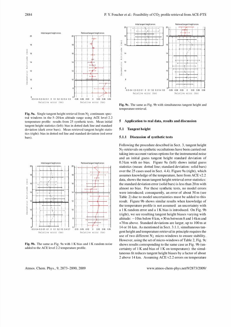
Fig. 10. Mean difference between N2-retrieved tangent height pro-
files and ACE v2.2 tangent heights from real occultation data for a
region of the Northern Hemisphere (50–70◦ N; 0–90◦ W). The red
curve represents the mean difference in July 2006 for 35 occulta-tions. The grey curve represents the mean difference in November
2006 for 40 occultations. For each case, error bars correspond to the
variance of the difference between ACE v2.2 tangent heights and
N2-retrieved tangent heights for the selected set of occultations.
profiles and on tangent heights (as they are correlated in the
case of real data), a simultaneous fit can markedly reduce
these errors in comparison with single tangent heights re-
trieval. This is especially significant for our purpose when
these errors are due to correlation with CO2 a priori profile
data.
5.1.2 First application to real data
These results are confirmed by looking at tangent height pro-
files retrieved from real ACE data for two months in 2006
(July and November). Figure 10 shows mean differences be-
tween N2-retrieved and ACE v2.2 tangent height profiles for
these two months for a region of the Northern Hemisphere
(50–70◦ N; 0–90◦ W). In July, the mean difference tangent
height profile increases from −20 m to 75 m from 6 to 11 km
and then decreases to +10 m at 18 km. In November the mean
difference tangent height profile is different: it regularly de-
creases from +125 m at 6 km to −20 m at 18 km. At 6 km thedifference between November and July is about 130 m while
it is about 30 m at 18 km. ACE v2.2 tangent height errors
due to correlation with CO2 a priori profile are expected to
be more important for lower altitudes because: (i) only CO2
transitions are used to fit tangent heights below 12 km, and
(ii) CO2 seasonal variations are known to be more important
at lower altitudes. ACE v2.2 tangent height retrieval sensi-
tivity to CO2 a priori concentration is of the order of 125 m
for a 5 ppm change, a value which corresponds well to the
change in CO2 concentration between summer and autumn
6
8
10
12
14
16
18
20
22
24
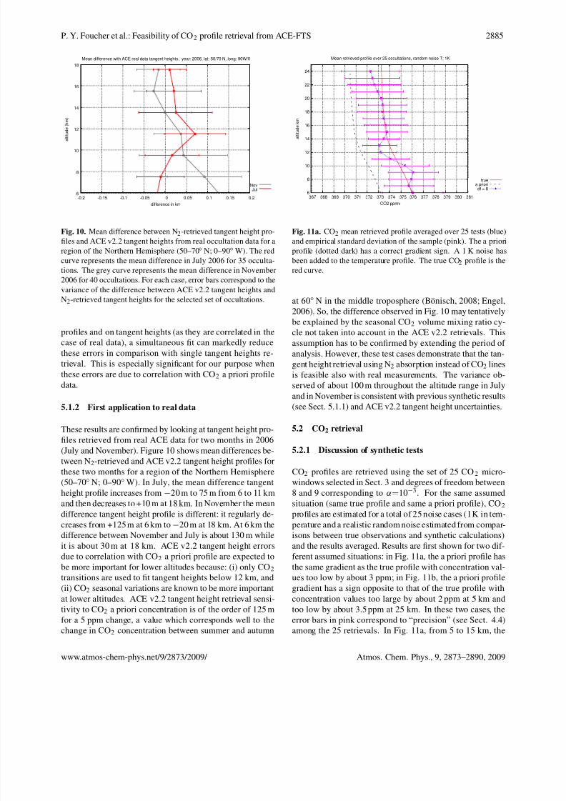
367 368 369 370 371 372 373 374 375 376 377 378 379 380 381
a l t i t u
d e k m
CO2 ppmv
Mean retrieved profile over 25 occultations, random noise T: 1K
truea prioridf = 8
Fig. 11a. CO2 mean retrieved profile averaged over 25 tests (blue)
and empirical standard deviation of the sample (pink). The a priori
profile (dotted dark) has a correct gradient sign. A 1 K noise has
been added to the temperature profile. The true CO2 profile is thered curve.
at 60◦ N in the middle troposphere (Bonisch, 2008; Engel,
2006). So, the difference observed in Fig. 10 may tentatively
be explained by the seasonal CO2 volume mixing ratio cy-
cle not taken into account in the ACE v2.2 retrievals. This
assumption has to be confirmed by extending the period of
analysis. However, these test cases demonstrate that the tan-
gent height retrieval using N2 absorption instead of CO2 lines
is feasible also with real measurements. The variance ob-
served of about 100 m throughout the altitude range in July
and in November is consistent with previous synthetic results(see Sect. 5.1.1) and ACE v2.2 tangent height uncertainties.
5.2 CO2 retrieval
5.2.1 Discussion of synthetic tests
CO2 profiles are retrieved using the set of 25 CO 2 micro-
windows selected in Sect. 3 and degrees of freedom between
8 and 9 corresponding to α=10−3. For the same assumed
situation (same true profile and same a priori profile), CO 2
profiles are estimated for a total of 25 noise cases (1K in tem-
perature and a realistic random noise estimated from compar-isons between true observations and synthetic calculations)
and the results averaged. Results are first shown for two dif-
ferent assumed situations: in Fig. 11a, the a priori profile has
the same gradient as the true profile with concentration val-
ues too low by about 3 ppm; in Fig. 11b, the a priori profile
gradient has a sign opposite to that of the true profile with
concentration values too large by about 2 ppm at 5 km and
too low by about 3.5 ppm at 25 km. In these two cases, the
error bars in pink correspond to “precision” (see Sect. 4.4)
among the 25 retrievals. In Fig. 11a, from 5 to 15 km, the
www.atmos-chem-phys.net/9/2873/2009/ Atmos. Chem. Phys., 9, 2873–2890, 2009
8/2/2019 P. Y. Foucher et al- Technical Note: Feasibility of CO2 profile retrieval from limb viewing solar occultation made by t…
http://slidepdf.com/reader/full/p-y-foucher-et-al-technical-note-feasibility-of-co2-profile-retrieval-from 14/18
2886 P. Y. Foucher et al.: Feasibility of CO2 profile retrieval from ACE-FTS
6
8
10
12
14
16
18
20
22
24
367 368 369 370 371 372 373 374 375 376 377 378 379 380 381
a l t i t u
d e k m
CO2 ppmv
Mean retrieved profile over 25 occultations, random noise T: 1K
truea prioridf = 8
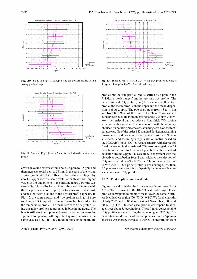
Fig. 11b. Same as Fig. 11a except using an a priori profile with a
wrong gradient sign.
6
8
10
12
14
16
18
20
22
24
367 368 369 370 371 372 373 374 375 376 377 378 379 380 381
a l t i t u d e k m
CO2 ppmv
Mean retrieved profile over 25 occultations, random noise T: 2K
true
a prioridf = 8
Fig. 12. Same as Fig. 11a with 2 K noise added to the temperature
profile.
error bar value decreases from about 2.5 ppm to 1.5 ppm and
then increases to 2.5 ppm to 25 km. In the case of the wrong
a priori gradient of Fig. 11b, error bar values are larger by
about 0.5 ppm with the same evolution with altitude (higher
values at top and bottom of the altitude range). For the twocases (Fig. 11a and b) the maximum absolute difference with
the true profile is about 1 ppm (due to spurious oscillations),
and no significant bias due to the a priori profile appears. In
Fig. 12, the same a priori and true profiles as Fig. 11a are
used and a 2 K temperature random noise has been added to
the temperature profile. The mean retrieved CO2 profile us-
ing this noisy profile is represented in blue in the figure. The
bias is still less than 1 ppm and error bar values increase by
1 ppm in comparison with Fig. 11a. Figure 13 considers the
same case as Fig. 11a (only random noise on temperature
6
8
10
12
14
16
18
20
22
24
367 368 369 370 371 372 373 374 375 376 377 378 379 380 381
a l t i t u
d e k m
CO2 ppmv
Mean retrieved profile over 25 occultations, random noise T: 1K
truea prioridf = 8
Fig. 13. Same as Fig. 11a with CO2 with a true profile showing a
4–5 ppm “hump” in the 9–13 km altitude range.
profile) but the true profile (red) is shifted by 5 ppm in the
9–13 km altitude range from the previous true profile. The
mean retrieved CO2 profile (blue) follows quite well the true
profile; the mean error is about 1 ppm and the mean disper-
sion is about 2 ppm. The two sharp steps from 13 to 14 km
and from 8 to 9 km of the true profile “hump” are less ac-
curately retrieved (maximum error of about 2.5 ppm). How-
ever, the retrieval can reproduce a 4 km thick CO2 profile
structure with a good vertical resolution. With the accuracy
obtained on pointing parameters, assuming errors on the tem-
perature profile of the order 1 K standard deviation, assuming
instrumental and model noise according to ACE-FTS mea-
surements, and assuming a regularization matrix based on
the MOZART model CO2 covariance matrix with degrees of
freedom around 9, the retrieved CO2 error averaged over 25
occultations comes to less than 1 ppm bias with a standard
deviation around 2 ppm. This accuracy is consistent with the
objectives described in Sect. 1 and validates the selection of
CO2 micro-windows (Table 3.2.1). The retrieval error due
to MOZART CO2 a priori profile is weak enough (less than
0.5 ppm) to allow averaging of spatially and temporally con-
sistent retrieved CO2 profiles.
5.2.2 First application to real data
Figure 14a and b display the first CO2 profiles retrieved from
ACE-FTS instrument in the 10–22 km altitude range. These
profiles correspond to monthly means over the same North-
ern Hemisphere region (50–70◦ N; 0–90◦ W) for the months
of July 2005 and 2006 (Fig. 14a) and November 2005 and
2006 (Fig. 14b). In each case, profiles correspond to aver-
ages over about 35 occultations. These figures correspond to
CO2 profiles retrieved using the isotopologue 12C16O2. The
mean standard deviation of the samples is around 2.5 ppm in
all cases. An average increase of the CO2 concentration from
Atmos. Chem. Phys., 9, 2873–2890, 2009 www.atmos-chem-phys.net/9/2873/2009/
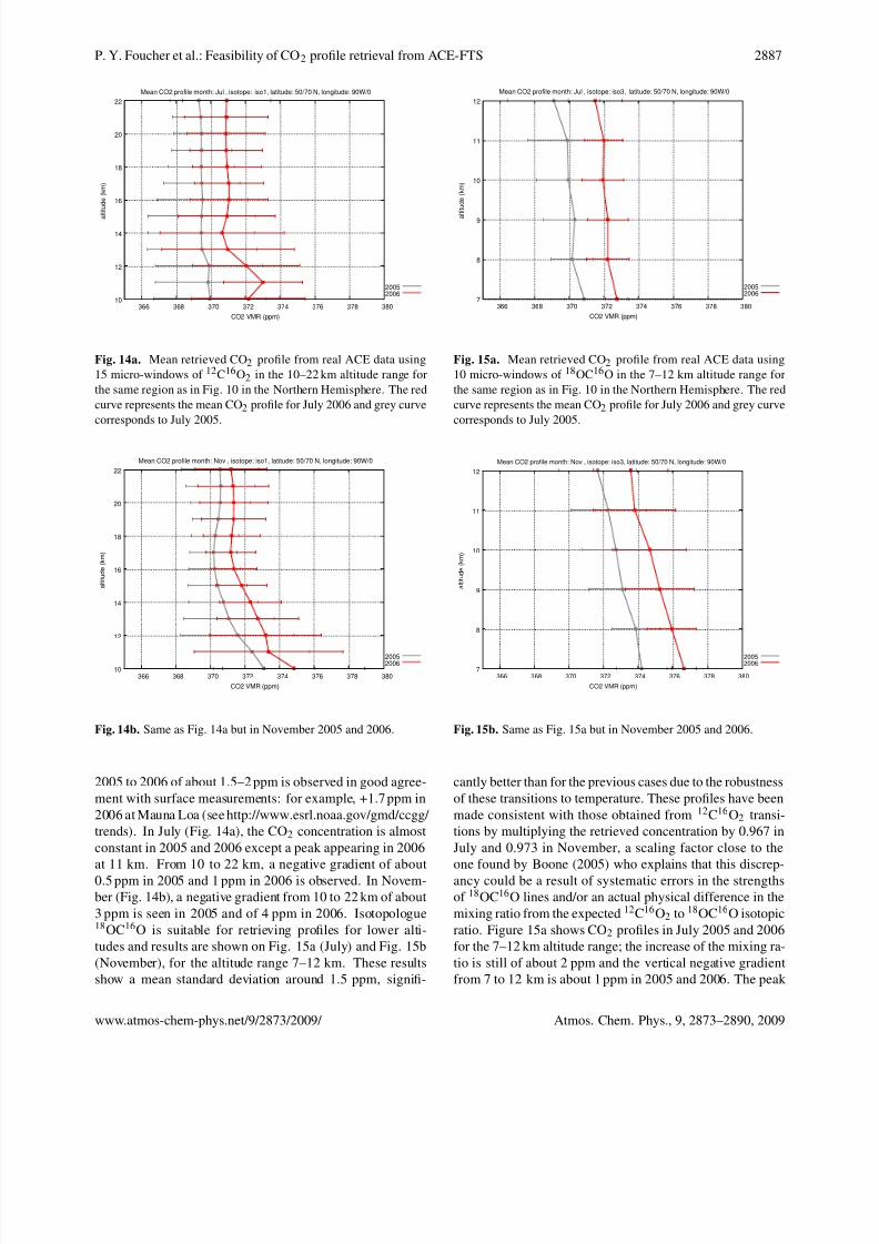
8/2/2019 P. Y. Foucher et al- Technical Note: Feasibility of CO2 profile retrieval from limb viewing solar occultation made by t…
http://slidepdf.com/reader/full/p-y-foucher-et-al-technical-note-feasibility-of-co2-profile-retrieval-from 15/18
P. Y. Foucher et al.: Feasibility of CO2 profile retrieval from ACE-FTS 2887
10
12
14
16
18
20
22
366 368 370 372 374 376 378 380
a l t i t u d
e ( k m )
CO2 VMR (ppm)
Mean CO2 profile month: Jul , isotope: iso1, latitude: 50/70 N, longitude: 90W/0
20052006
Fig. 14a. Mean retrieved CO2 profile from real ACE data using
15 micro-windows of 12C16O2 in the 10–22 km altitude range for
the same region as in Fig. 10 in the Northern Hemisphere. The red
curve represents the mean CO2 profile for July 2006 and grey curvecorresponds to July 2005.
10
12
14
16
18
20
22
366 368 370 372 374 376 378 380
a l t i t u d e ( k m )
CO2 VMR (ppm)
Mean CO2 profile month: Nov , isotope: iso1, latitude: 50/70 N, longitude: 90W/0
20052006
Fig. 14b. Same as Fig. 14a but in November 2005 and 2006.
2005 to 2006 of about 1.5–2 ppm is observed in good agree-
ment with surface measurements: for example, +1.7 ppm in
2006 at Mauna Loa (see http://www.esrl.noaa.gov/gmd/ccgg/ trends). In July (Fig. 14a), the CO2 concentration is almost
constant in 2005 and 2006 except a peak appearing in 2006
at 11 km. From 10 to 22 km, a negative gradient of about
0.5 ppm in 2005 and 1 ppm in 2006 is observed. In Novem-
ber (Fig. 14b), a negative gradient from 10 to 22 km of about
3 ppm is seen in 2005 and of 4 ppm in 2006. Isotopologue18OC16O is suitable for retrieving profiles for lower alti-
tudes and results are shown on Fig. 15a (July) and Fig. 15b
(November), for the altitude range 7–12 km. These results
show a mean standard deviation around 1.5 ppm, signifi-
7
8
9
10
11
12
366 368 370 372 374 376 378 380
a l t i t u d
e ( k m )
CO2 VMR (ppm)
Mean CO2 profile month: Jul , isotope: iso3, latitude: 50/70 N, longitude: 90W/0
20052006
Fig. 15a. Mean retrieved CO2 profile from real ACE data using
10 micro-windows of 18OC16O in the 7–12 km altitude range for
the same region as in Fig. 10 in the Northern Hemisphere. The red
curve represents the mean CO2 profile for July 2006 and grey curvecorresponds to July 2005.
7
8
9
10
11
12
366 368 370 372 374 376 378 380
a l t i t u d e ( k m )
CO2 VMR (ppm)
Mean CO2 profile month: Nov , isotope: iso3, latitude: 50/70 N, longitude: 90W/0
20052006
Fig. 15b. Same as Fig. 15a but in November 2005 and 2006.
cantly better than for the previous cases due to the robustness
of these transitions to temperature. These profiles have been
made consistent with those obtained from12
C16
O2 transi-tions by multiplying the retrieved concentration by 0.967 in
July and 0.973 in November, a scaling factor close to the
one found by Boone (2005) who explains that this discrep-
ancy could be a result of systematic errors in the strengths
of 18OC16O lines and/or an actual physical difference in the
mixing ratio from the expected 12C16O2 to 18OC16O isotopic
ratio. Figure 15a shows CO2 profiles in July 2005 and 2006
for the 7–12 km altitude range; the increase of the mixing ra-
tio is still of about 2 ppm and the vertical negative gradient
from 7 to 12 km is about 1 ppm in 2005 and 2006. The peak
www.atmos-chem-phys.net/9/2873/2009/ Atmos. Chem. Phys., 9, 2873–2890, 2009
8/2/2019 P. Y. Foucher et al- Technical Note: Feasibility of CO2 profile retrieval from limb viewing solar occultation made by t…
http://slidepdf.com/reader/full/p-y-foucher-et-al-technical-note-feasibility-of-co2-profile-retrieval-from 16/18
2888 P. Y. Foucher et al.: Feasibility of CO2 profile retrieval from ACE-FTS
seen at 11 km on Fig. 14a is not seen here. Figure 15b shows
CO2 profiles in November 2005 and 2006 for the same alti-
tude range; the mixing ratio again increases by about 2 ppm
and the vertical negative gradients are close to the one ob-
served on Fig. 14b. In conclusion, these preliminary results
obtained from real occultations show a CO2 concentration
trend close to the one measured in situ and a vertical gradient
in July and November consistent with aircraft measurementcampaigns (Engel, 2006; Sawa, 2008).
6 Conclusions and future work
Accurate temporal and spatial determination of CO2 concen-
tration profiles is of great importance for the improvement
of air transport models. Coupled with column measurements
from a nadir instrument, occultation measurements will also
bring useful constraints to the surface carbon flux determi-
nation (Pak , 2001; Patra, 2003), for example, by indicating
what portion of the column measurement comes from the re-gion below 5 km.
In this paper we have shown that, in contrast to present
and near future satellite observations of the distribution of
CO2, which provide vertically integrated concentrations, the
high spectral resolution and signal to noise ratio of the so-
lar occultation measurements of the ACE-FTS instrument on
board SCISAT are able to provide CO2 vertical profiles in the
5–25 km altitude range. The major difficulty, when apply-
ing a conventional method where the tangent heights point-
ing information is retrieved from CO2 transitions is the cor-
relation which exists between the pointing parameters (tan-
gent heights of measurements and temperature profiles) and
a CO2 a priori profile in this altitude range. This problem
has been solved using, for the first time, the N2 collision-
induced absorption continuum near 2500 cm−1. Its high sen-
sitivity to altitude leads to an estimated precision less than
100 m for the tangent height N2-retrieval. These results are
confirmed by first retrievals from real ACE-FTS data. More-
over, in the 5–25 km altitude range, the selection of CO2 lines
with low values of the lower state energy value E makes the
CO2 retrieval quite insensitive to temperature uncertainties.
A comprehensive analysis of the errors (estimated from real
data) introduced by the instrument, spectroscopy, interfering
species, and temperature has resulted in the selection of a set
of 25 CO2 micro-windows. The use of an optimized regu-larization matrix based on a CO2 covariance matrix calcu-
lated from the MOZART model ensures good convergence
of the non-linear iterative retrieval method with an accept-
able number of degrees of freedom and a vertical resolution
around 2 km. The estimated CO2 total error shows a bias of
about 1 ppm with a standard deviation of about 2 ppm after
averaging over 25 spatially and temporally consistent pro-
files. These synthetic results, simulating realistic conditions
of observation, and the first CO2 vertical profiles retrieved
from real occultations shown in this paper are very encour-
aging as they basically match our present knowledge. The
method will soon be applied to the whole ACE-FTS archive
providing, for the first time, CO2 vertical profiles in the 5–
25 km altitude range over a period of more than 4 years on a
near global scale.
One remaining issue that will need to be solved is the use
of 18OC16O lines near 2610 cm for the lowest altitudes and
13C16O2 lines near 2020 cm in the retrieval. The ratio of iso-topologues concentrations in the atmosphere can vary from
the standard abundance value assumed for the line intensi-
ties in the spectroscopic databases, especially the ratio of 18OC16O to 12C16O2 concentration. However, the consis-
tency seen between profiles retrieved from real data using ei-
ther 18OC16O lines for the 7–12 km altiude range or 12C16O2
lines for the 10–22 km is very encouraging.
Acknowledgements. We gratefully acknowledge R. Armante, C.
Crevoisier, B. Legras and N. A. Scott for fruitful discussions, help
and constructive criticisms.
The ACE mission is supported primarily by the Canadian Space
Agency (CSA) and some support was provided by the Natural
Environment Research Council (NERC) of the UK.
Edited by: R. Sander
The publication of this article is financed by CNRS-INSU.
References
Anderson, B., Gregory, G., Collins, J. J., Sachse, G., Conway, T.,
and Whiting, G.: Airborne observations of spatial and temporal
variability of tropospheric carbon dioxide, J. Geophys. Res., 101,
1985–1997, 1996.
Andrew, A. E., Boering, K. A., Daube, B. C.,Wofsy, S. C., Loewen-
stein, M., Jost, H., Podolske, J. R.,Webster, C. R., Herman, R.
L., Scott, D. C., Flesch, G. J., Moyer, E. J., Elkins, J. W., Dutton,
G. S., Hurst, D. F., Moore, F. L., Ray, E. A., Romashkin, P. A.,
and Strahan, S. E.: Mean ages of stratospheric air derived from
in situ observations of CO2, CH4, and N2O, J. Geophys. Res.,106, 32295–32314, 2001.
Baker, D. F., Law, R. M., Gurney, K. R., Rayner, P., Peylin, P.,
Denning, A. S., Bousquet, P., Bruhwiler, L., Chen, Y. H., Ciais,
P., Fung, I. Y., Heimann, M., John, J., Maki, T., Maksyutov,
S., Masarie, K., Prather, M., Pak, B., Taguchi, S., and Zhu,
Z.: TransCom3 inversion intercomparison: Interannual variabil-
ity of regional CO2 fluxes, Global Biogeochem. Cy., 1988–2003,
doi:10.1029/2004GB002439, 2006.
Bernath, P. F.: Atmospheric Chemistry Experiment (ACE): Analyt-
ical Chemistry from Orbit, Trends Anal. Chem., 25, 647–654,
2006.
Atmos. Chem. Phys., 9, 2873–2890, 2009 www.atmos-chem-phys.net/9/2873/2009/
8/2/2019 P. Y. Foucher et al- Technical Note: Feasibility of CO2 profile retrieval from limb viewing solar occultation made by t…
http://slidepdf.com/reader/full/p-y-foucher-et-al-technical-note-feasibility-of-co2-profile-retrieval-from 17/18
P. Y. Foucher et al.: Feasibility of CO2 profile retrieval from ACE-FTS 2889
Bernath, P. F., McElroy, C. T., Abrams, M. C., Boone, C. D., Butler,
M., Camy-Peyret, C., Carleer, M., Clerbaux, C., Coheur, P.-F.,
Colin, R., DeCola, P., DeMaziere, M., Drummond, J. R., Dufour,
D., Evans, W. F. J., Fast, H., Fussen, D., Gilbert, K., Jennings, D.
E., Llewellyn, E. J., Lowe, R. P., Mahieu, E., Mc- Connel, J. C.,
McHugh, M., Mcleod, S. D., Michaud, R., Midwinter, C., Nas-
sar, R., Nichitiu, F., Nowland, C., Rinsland, C. P., Rochon, Y. J.,
Rowlands, N., Semeniuxk, K., Simon, P., Skelton, R., Sloan, J. J.,
Soucy, M. A., Strong, K., Tremblay, P., Turnbull, D., Walker, K.
A., Walkty, I., Wardle, D. A., Wehrle, V., Zander, R., and Zou, T.:
Atmospheric Chemistry Experiment (ACE): Misson overview,
Geophys. Res. Lett., 32, L15S01, doi:10.1029/2005GLO22386,
2005.
Bonisch, H., Hoor, P., Gurk, C., Feng, W., Chipperfield, M., En-
gel, A., and Bregman, B.: Model evaluation of CO2 and SF6 in
the extratropical UT/LS region, J. Geophys. Res., 113, D06101,
doi:10.1029/2007JD008829, 2008.
Boone, C. D., Nassar, R.,Walker, K. A., Rochon, Y., Mcleod, S.
D., Rinsland, C. P., and Bernath, P. F.: Retrievals for the Atmo-
spheric Chemistry Experiment Fourier-Transform Spectrome-
trer, Appl. Opt., 44, 7218–7231, 2005.
Brenninkmeijer, C. A. M., Crutzen, P. J., Fischer, H., Gsten, H.,Hans, W., Heinrich, G., Heintzenberg, J., Hermann, M., Im-
melmann, T., Kersting, D., Maiss, M., Nolle, M., Pitscheider,
A., Pohlkamp, H., Scharffe, D., Specht, K., and Wiedensohler,
A.: CARIBIC: Civil Aircraft for Global Measurement of Trace
Gases and Aerosols in the Tropopause Region, J. Atmos. Ocean.
Tech., 16, 1373–1383, 1999.
Buchwitz, M., de Beek, R., Noel, S., Burrowsandi, J. P., Bovens-
mann, H., Bremer, H., Bergamaschi, P., Krner, S., and Heimann,
M.: Carbon monoxide, methane and carbon dioxide columns re-
trieved from SCIAMACHY by WFM-DOAS: year 2003 initial
data set., Atmos. Chem. Phys., 5, 3313–3329, 2005,
http://www.atmos-chem-phys.net/5/3313/2005/.
Chedin, A., Serrar, S., Armante, R., Scott, N. A., and
Hollingsworth, A.: Signatures of annual and seasonal variations
of CO2and other greenhouse gases from comparisons between
NOAA/TOVS observations and model simulations, J. Clim., 15,
95–116, 2002.
Chedin, A., Serrar S., Scott, N. A., Crevoisier, C., and Armante, R.:
First global measurement of mid-tropospheric CO2 from NOAA
polar satellites : the tropical zone, J. Geophys. Res., 108, 4581,
doi:10.1029/2003JD003439, 2003a.
Chedin, A., Saunders, R., Hollingsworth, A., Scott, N. A., Ma-
tricardi, M., Etcheto, J., Clerbaux, C., Armante, R., and
Crevoisier, C.: The feasibility of monitoring CO2 from high-
resolution infrared sounders, J. Geophys. Res., 108, 4064,
doi:10.1029/2001JD00144, 2003b.
Crevoisier, C., Heilliette, S., Chedin, A., Serrar, S., Armante, R.,and Scott, N. A.: Midtropospheric CO2 concentration retrieval
from AIRS observations in the tropics, Geophys. Res. Lett., 31,
L17106, doi:10.1029/2004GL020141, 2004.
Dudhia, A., Jay, V. L., and Rodgers, C. D.: Microwindow selec-
tion for high-spectral-resolution sounders, Appl. Opt., 41, 3665–
3673, 2002.
Engel, A., Bonish, H., Brunner, D., Fischer, H., Franke, H., Gunter,
G., Gurk, C., Hegglin, M., Hoor, P., Konigstedt, R., Krebach,
M., Maser, R., Parchatka, U., Peter, T., Schell, D., Schiller,
C., Schmidt, U., Spelten, N., Szabo, T., Weers, U., Wernli, H.,
Wetter, T., and Wirth, V.: Highly resolved observations of trace
gases in the lowermost stratosphere from the Spurt project: an
overview, Atmos. Chem. Phys., 6, 283–301, 2006,
http://www.atmos-chem-phys.net/6/283/2006/.
Engelen, R. J. and McNally, A. P.: Estimating atmospheric
CO2from advanced infrared satellite radiances within an oper-
ational four-dimensional variational (4D-Var) data assimilation
system: Results and validation, J. Geophys. Res., 110, D18305,
doi:10.1029/2005JD005982, 2005.
Gelb, A.: Applied Optimal Estimation, M.I.T. Press, 180–229,
1974.
Gurney, K. R., Law, R. M., Denning, A. S., Rayner, P. J., Baker,
D., Bousquet, P., Bruhwiler, L., Chen, Y. H., Ciais, P., Fan, S.,
Fung, I. Y., Gloor, M., Heimann, M., Higuchi, K., John, J., Maki,
T., Maksyutov, S., Masarie, K., Peylin, P., Prather, M., Pak, B.
C., Randerson, J., Sarmiento, J., Taguchi, S., Takahashi, T., and
Yuen, C. W.: Towards robust regional estimates of CO2 sources
and sinks using atmospheric transport models, Nature, 415, 626–
630, 2002.
Hegglin, M. I., Boone, C. D., Manney, G. L., Shephered, T. G.,
Walker, K. A., Bernath, P. F., Daffer, W. H., Hoor, P., and
Schiller, C.: Validation of ACE-FTS satellite data in the up-per troposphere/lower stratosphere (UTLS) using non-coincident
measurements, Atmos. Chem. Phys., 8, 1483–1499, 2008,
http://www.atmos-chem-phys.net/8/1483/2008/ .
Horowitz, L. W., Walters, S., Mauzerall, D. L., Emmons, L. K.,
Rasch, P. J., Granier, C., Tie, X., Lamarque, J. F., Schultz, M.
G., Tyndall, G. S., Orlando, J. J., and Brasseu, G. P.: A global
simulation of tropospheric ozone and related tracers: Description
and evaluation of MOZART, version 2, J. Geophys. Res., 108,
4784, doi:10.1029/2002JD002853, 2003.
Jacquinet-Husson, N., Scott, N. A., Chedin, A., Crepeau, L., Ar-
mante, R., Capelle, V., Orphal, J., Coustenis, A., Boonne, C.,
Poulet-Crovisier, N., Barbe, A., Birk, M., Brown, L. R., Camy-
Peyret, C., Claveau, C., Chance, K., Christidis, N., Clerbaux,
C., Coheur, P. F., Dana, V., Daumont, L., Backer-Barilly, M.
R. D., Lonardo, G. D., Flaud, J. M., Goldman, A., Hamdouni,
A., Hess, M., Hurley, M. D., Jacquemart, D., Kleiner, I., Kpke,
P., Mandin, J. Y., Massie, S., Mikhailenko, S., Nemtchinov, V.,
Nikitin, A., Newnham, D., Perrin, A., Perevalov, V., Pinnock, S.,
Rgalia-Jarlot, L., Rinsland, C., Rublev, A., Schreier, F., Schult,
L., Smithu, K. M., Tashkun, S. A., Teffo, J. L., Toth, R. A.,
Tyuterev, V. G., Auwera, J. V., Varanasi, P., and Wagner, G.:
The GEISA spectroscopic database: Current and future archive
for Earth and planetary atmosphere studies, JQSRT, 100, 1043–
1059, 2008.
Koner, P. K. and Drummond, J. R.: Atmospheric trace
gases profile retrievals using the nonlinear regularized
total least square method, JQSRT, 109, 2045–2059,doi:10.1016/j.jqsrt.2008.02.014, 2008.
Lafferty, W. J., Solodov, A. M., Weber, A., Olson, W. B., and Hart-
mann, J.-M.: Infrared collision-induced absorption by N2 near
4.3µm for atmospheric applications: measurements and empiri-
cal modeling, Appl. Opt., 35, 5911–5917, 1996.
Levenberg, K. :A Method for the Solution of Certain Non-Linear
Problems in Least Squares. The Quarterly of Applied Mathemat-
ics, 2, 164–168, 1944.
Matsueda, H., Taguchi, S., Inoue, H. Y., and Ishii, M.: A large
impact of tropical biomass burning on CO and CO2 in the upper
www.atmos-chem-phys.net/9/2873/2009/ Atmos. Chem. Phys., 9, 2873–2890, 2009
8/2/2019 P. Y. Foucher et al- Technical Note: Feasibility of CO2 profile retrieval from limb viewing solar occultation made by t…
http://slidepdf.com/reader/full/p-y-foucher-et-al-technical-note-feasibility-of-co2-profile-retrieval-from 18/18
2890 P. Y. Foucher et al.: Feasibility of CO2 profile retrieval from ACE-FTS
troposphere, Science China Press, 45, 116–125, 2002.
Marquardt, D.: An Algorithm for Least-Squares Estimation of
Nonlinear Parameters. SIAM J. Appl. Math., 11, 431–441,
doi:10.1137/0111030, 1963.
Olsen, S. C. and Randerson, J. T.: Differences between sur-
face and column atmospheric CO2 and implications for
carbon cycle research, J. Geophys. Res., 109, D02301,
doi:10.1029/2003JD003968, 2004.
Pak, B. C. and Prather, M. J.: CO2 source inversions using satellite
observations of the upper troposphere, Geophys. Res. Lett., 28,
4571–4574, 2001.
Park, J. H.: Atmospheric CO2 monitoring from space, Appl. Opt.,
36, 2701–2712, 1997.
Patra, P. K., Maksyutov, S., Sasano, Y., Nakajima, H., Inoue, G.,
and Nakazawa, T.: An evaluation of CO2 observations with
Solar Occultation FTS for Inclined-Orbit Satellite sensor for
surface source inversion, J. Geophys. Res., 108(D24), 4759,
doi:10.1029/2003JD003661, 2003.
Phillips, D. L.:A Technique for the Numerical Solution of Certain
Integral Equations of the First Kind, J. Assoc. Comput. Mach.,
9, 84–97, 1962.
Plumb, R.: A “tropical pipe” model of stratospheric transport, J.Geophys. Res., 301, 3957–3972, 1996.
Plumb, R. and Ko, M.: Interrelationships between mixing ratios
of long-lived stratosphere constituents, J. Geophys. Res., 97,
10145–10156, 1992.
Rodgers, C. D.: Inverse methods for atmospheric sounding. Theory
and practice, World scientific, Singapore, 90–98, 2000.
Sawa, Y. , Machida, T. and Matsueda, H.: Seasonal variations of
CO2 near the tropopause observed by commercial aircraft, J.
Geophys. Res., 113, D23301, doi:10.1029/2008JD010568, 2008.
Scott, N. A.: A direct method of computation of transmission func-
tion of an inhomogeneous gaseous medium : description of the
method and influence of various factor, JQSRT, 14, 691–707,
1974.
Scott, N. A. and Chedin, A.: A fast line-by-line method for atmo-
spheric absorption computation: The Automatized Atmospheric
Absorption Atlas, J.Appl.Meteorol., 20, 801–812, 1981.
Shia, R. L., Liang, M. C., Miller, C. E., and Yung, Y.
L.: CO2 in the upper troposphere: Influence of strato-
spheretroposphere exchange, Geophys. Res. Lett., 33, L1481,
doi:10.1029/2006GL026141, 2006.
Steck, T.: Methods for determining regularization for atmospheric
retrieval problems, Appl. Opt., 41, 1788-1797, 2002.
Tikhonov, A. N.: On the regularization of ill-posed problems. Dokl.
Akad. Nauk SSSR, 153, 49–52; MR, 28, 5577; Soviet Math.
Dokl., 4, 1624–1627, 1963.
Twomey, S.: On the Numerical Solution of Fredholm Integral Equa-
tions of the First Kind by the Inversion of the Linear System Pro-
duced by Quadrature, J. Assoc. Comp. Mach., 10, 97–101, 1963.
von Clarmann, T. and Echle, G.: Selection of optimized microwin-
dows for atmospheric spectroscopy, Appl. Opt., 37, 7661–7669,
1998.von Clarmann, T., Glatthor, N., Grabowski, U., Hopfner, M., Kell-
mann, S., Kiefer, M., Linden, A., Tsidu, G. M., Milz, M., Steck,
T., Stiller, G. P., Wang, D. Y., Fischer, H., Funke, B., and Gil-
Lopez-Puerta, S.: Retrieval of temperature and tangent altitude
pointing from limb emission spectra recorded from space by
the Michelson Interferometer for Passive Atmospheric Sounding
(MIPAS), J. Geophys. Res., 108, 4736–4750, 2003.
A Ch Ph 9 2873 2890 2009 h h /9/2873/2009/