p rotein seondary & super-secondary structure prediction with hmm by en-shiun annie lee cs 882...

PROTEIN SEONDARY & SUPER-SECONDARY

STRUCTURE PREDICTION

WITH HMMBy En-Shiun Annie Lee

CS 882 Protein Folding

Instructed by Professor Ming Li

1. Introduction

2. Problem

3. Methods (4)

4. HMM Examples (3)a. Segmentation HMMb. Profile HMMc. Conditional Random Field

5. Proposal

0. OUTLINE

1. Introduction *

2. Problem

3. Methods (4)


5. Proposal

1. INTRODUCTION

• Achievements in Genomic– BLAST

(Basic Local Alignment Search Tool) • most cited paper published in 1990s• more than 15,000 times

– Human genome project• Completion April 2003

1. Genomics

• Precedence to Proteomics– Protein Data Bank (PDB)

• 40,132 structures• cited more than 6,000 times

1. Proteomics

1. ProteomicsNumber of Protein Structures in Protein Data Bank

• Importance– The known secondary structure may be used as an input for the

tertiary structure predictions.

1. Secondary Structure

• Primary Structure

1. Protein Structure

• Secondary Structure


1. Secondary Structure• α-helix

– Interaction between i and (i+4)th residue

1. Secondary Structure• β-sheet/strand

– Parallel or Anti-parallel

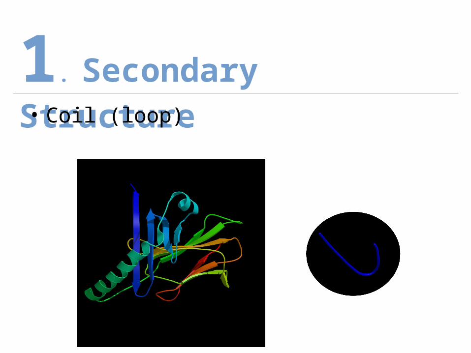
1. Secondary Structure• Coil (loop)

• Tertiary Structure


• Super-Secondary (2.5) Structure


Super-Secondary (2.5)

Structure

• Quaternary Structure


Super-Secondary (2.5)

Structure

1. Introduction

2. Problem *

3. Methods (4)


5. Proposal

2. PROBLEM

• Problem– Given:

• A primary sequence of amino acids– a1a2…an

– Find: • Secondary structure of each ai as

– α-helix = H– β-strand = E *– coil = C


• Example– Given:

• Primary Sequence– GHWIATRGQLIREAYEDYRHFSSECPFIP

– Find:• Secondary Structure Element

– CEEEEECHHHHHHHHHHHCCCHHCCCCCC– Note: segments


• Three-state prediction accuracy– Q3 = # of correctly predicted residues

total # of number of residues

– Q, Qβ, Qc

– Q3 for random prediction is 33%

– Theoretical limit Q3=90%.

2. Prediction Quality

• Segment Overlap (SOV)– Higher penalties for core segment regions

• Matthews Correlation Coefficients (MCC)– Prediction errors made for each state

2. Prediction Quality

• Three dimensional PDB data– DSSP (Dictionary of Secondary Structure of Proteins)

• 8 states– H = alpha helix H– G = 310 - helix H– I = 5 helix (pi helix) H– E = extended strand (beta ladder) E– B = residue in isolated beta-bridge E– T = hydrogen bonded turn C– S = bend C– C = coil C

– STRIDE

2. True Structures

1. Introduction

2. Problem

3. Methods (4) *


5. Proposal

3. METHODS

• Sliding-Window

3. Sliding Window

a. Statistical Methodb. Neural Networkc. Support Vector Machined. Hidden Markov Model

3. Four Methods

• Propensity

• Ex. Chou-Fasman 50~53%

3a. Statistical Method

• Ex. PHD 71%

3b. Neural Network

• Ex. PSIPRED 76~78%

3c. SVM

• State set Q• Output alphabet Σ

3d. HMM Definition

• Transition probabilities – probability of entering the state p from state q

– Tq(p) q Q p Q

3d. HMM Definition

• Emission probabilities – probability emits each letter of Σ from state q

– Eq(ai) ai Σ q Q

3d. HMM Definition

• Problem– Given:

• HMM = (Q,Σ,E,T) and• Sequence S

– Where S = S1, S2, …, Sn

– Find:• Most probable path of state gone through to get S

– Where X = X1, X2, …, Xn = state sequence

3d. HMM Decoding

• Optimize– Pr [ S , X ]

• X = X1, X2, …, Xn = state sequence

• S = S1, S2, …, Sn

– Pr [ S | X ]

4. HMM Decoding

• Dynamic programming– Memoryless– Pr [Xn|Sn] = Pr [Xn-1|Sn-1] Tn-1[Xn] EXn [Sn]

4. HMM Decoding

1. Introduction

2. Problem

3. Methods (4)

4. HMM Examples (3) *a. Segmentation HMMb. Profile HMMc. Conditional Random Field

5. Proposal

4. HMM EXAMPLES

1. Introduction

2. Problem

3. Methods (4)

4. HMM Examples (3)a. Semi-HMM *b. Profile HMMc. Conditional Random Field

5. Proposal

4a. SEMI-HMM

• Definition– Each state can emit a sequence– Move emission probabilities into states– Model secondary structure segments

4a. Semi-HMM

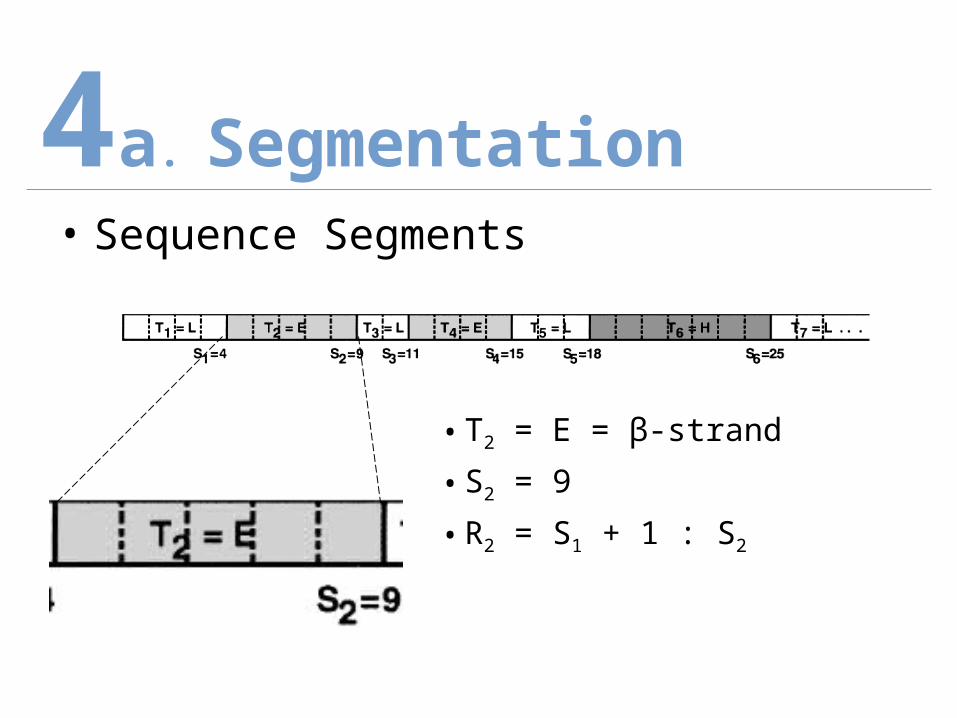
• Sequence Segments

4a. Segmentation


4a. Segmentation

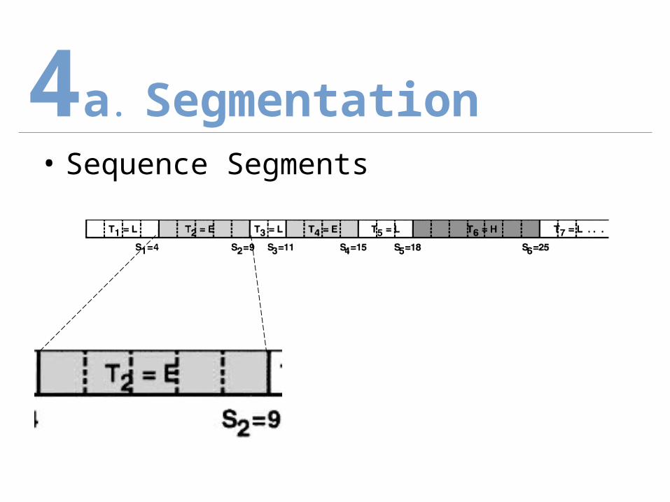
• T = secondary structural type of the segment, {H, E, L}

• S = ends of each individual structural segments

• R = known amino acid sequence


4a. Segmentation

• T2 = E = β-strand

• S2 = 9

• R2 = S1 + 1 : S2

• R = Sequence of ALL amino acid residues• S = End of the segments • T = Secondary structural type of the segments

– {H, E, L}

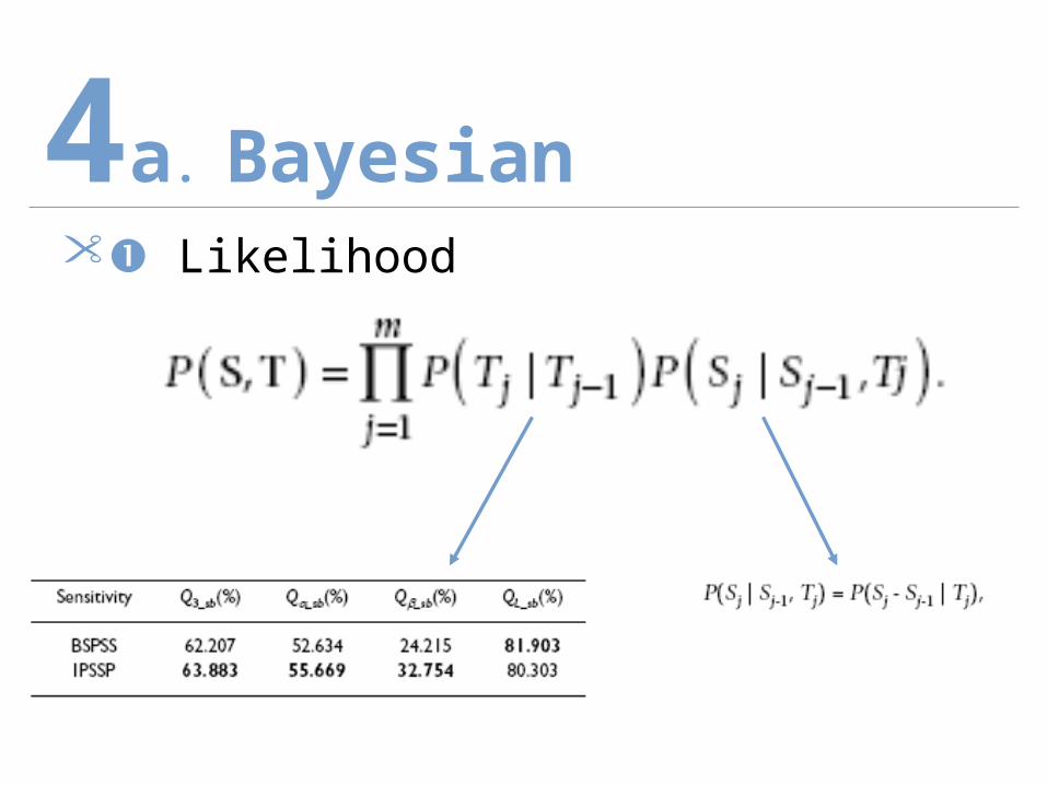
4a. Bayesian• Bayesian Formulation

1. Likelihood2. Priori Probability3. Constant (S,T) dropped

4a. Bayesian

• Bayesian Formulation

• m = Total number of segments

• Sj = End of the jth segments

• Tj = Secondary structural type of the jth segments

4a. Bayesian Likelihood


N-terminus

Internal

C-terminus

4a. BSPPS• Bayesian Segmentation PPS

4a. Results• Better than PSIPRED

– (w/o homology information)

1. Introduction

2. Problem

3. Methods (4)

4. HMM Examples (3)a. Semi-HMMb. Profile HMM *c. Conditional Random Field

5. Proposal

4b. PROFILE-HMM

• Main States– Columns of alignment

4b. Profile HMM

• Insertion States

4b. Profile HMM

• Deletion States– Jump over 1+ column in alignment

4b. Profile HMM

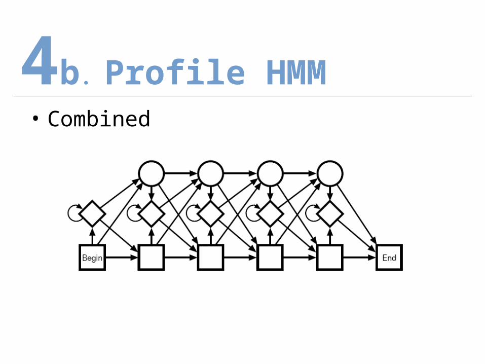
• Combined

4b. Profile HMM

• HMM for local protein STRucture

4b. HMMSTR

• HMM for local protein STRucture• Pronounced “hamster”

4b. HMMSTR

• I-sites Library – Motif = short basic structural fragments

• 3~19 residues• 262 motifs• Highly predictable

– Non-redundant PDB data (<25% similarity)– Fold uniquely across protein family– Exhaustive motif clustering

4b. I-Site Library

• States– Amino acid sequence and – Structural attribute

• Transition from state– Adjacent positions in motif– No gap or insertion states

4b. Build HMM

• Emission probability distributions– b = observed amino acid

• (20 probability values)

– d = secondary structure• (helix, strand, loop)

– r = backbone angle region • (11 dihedral angle symbols)

– c = structural context descriptor• (10 context symbols)

4b. Build HMM

• Model I-site Library– Each 262 motif is a chain in HMM– Merge states base on similarity of

• Sequence• Structure

4b. Build HMM

• Model I-site Library• Merge states

– base on similarity of• Sequence• Structure

4b. Build HMM

• Ex. β-Hairpin

4b. HMMSTR Merge

Serine β-Hairpin Type-I β-Hairpin

• Ex. β-Hairpin

4b. HMMSTR Merge

• Input: PDB proteins• Find

– best state sequence for sequence– probability distribution of one amino acid

• Integrate 3 data set– Aligned probability distribution– Amino acid and context information– Contact map

4b. HMMSTR Training

4b. HMMSTR Summary• 282 nodes

• 317 transitions• 31 merged motifs

• Introduce structural context on level of super-secondary structure• Predict higher-order 3D tertiary structure

– Side-result = predict 1D secondary structure

4b. HMMSTR Summary

1. Introduction

2. Problem

3. Methods (4)

4. HMM Examples (3)a. Semi-HMMb. Profile HMMc. Conditional Random Field *

5. Proposal

4b. PROFILE-HMM

• Does not model– Multiple interacting features– Long-range dependencies

• Strict independence assumptions

4c. HMM Disadvantages

• Allow– Arbitrary features– Non-independent features

• Transition probability– With respect to past and future observations

4c. Conditional Model

4c. Conditional Model

y1

x1

y2

x2

y3

x3

y4

x4

y5

x5

y6

x6

…HMM

y1

x1

y2

x2

y3

x3

y4

x4

y5

x5

y6

x6

…CRF

• Random Field (Undirected graphical model)– Let G = (Y, E) be a graph

• Where each vertex Yv = a random variable

– If P(Yv|all other Y)= P(Yv|neighbours of Yv)Then Y is a random field

4c. Random Field

• Example:– P(Y5 | all other Y) = P(Y5 | Y4, Y6)

4c. Random Field

• Conditional Random Field– Let X = r.v. data sequences to be labeled

• observations

– Let Y = r.v. corresponding label sequences• labels

– Let G = (V, E) be a graph • S.t. Y = (Yv)vY so Y is indexed by vertices of G

– If P(Yv | X, Yw w≠v) = P(Yv | X, Yw, w~v)Then (X, Y) is a random field

4c. Conditional RF

• Example:– P(Y3 | X, all other Y) = P(Y3 | X, Y2, Y4)

4c. Conditional RF

• HMM: – Maximize P(x,y|θ)=P(y|x,θ)P(x|θ)– Transition and emission probabilities– Transition/emission base only one x

• CRF: – Maximize P(y|x,θ)– Feature function f(i, j, k) – Feature function base on all x

4c. HMM vs. CRF

4c. Beta-Wrap• β-Helix

– 3 parallel β-strands– Connected by coils

• Few solved structures– 9 SCOP SuperFamilies– 14 RH solved structures in PDB – Solved structures differ widely

• Let G = (V,E1,E2) be a graph– V = Nodes/States = Secondary structures– Edges = interactions

• E1

– Edges between adjacent neighbors– Implied in the model

• E2

– Edges for long-term interactions– Explicitly considered

4c. Graph Definition

• Simple Example:– S2 = first β-strand – S3 = coil– S4 = second β-strand – S5 = coil– S6 = -helix

4c. Beta-Wrap Example

4c. Beta-Wrap

• β-Helix Solution:

1. Introduction

2. Problem

3. Methods (4)


5. Proposal *

5. PROPOSAL

• Do not infer global interaction– i.e. Beta-sheet interactions

• Protein structure definition constraint

5. Difficulties

• Novel methods of secondary structure prediction– Model as Integer Programming

• Super-secondary structure prediction

5. Possible Future Work

• Professor Ming Li– Guidance in

• knowledge and • expertise

• Bioinformatics lab• Mentoring a “rookie”

• Class• Attention and listening

5.

Acknowledgement

p rotein seondary & super-secondary structure prediction with hmm by en-shiun annie lee cs 882...

Documents