p o distribute electronically
TRANSCRIPT
Permission To Distribute Electronically
On Wed Feb. 12, 1997 I wrote John Kimmel (Senior Editor, Statistics, Springer-Verlag):
To: [email protected] Wed Feb 12 15:46:38 1997
Dear Mr. Kimmel,
About 9 years ago I wrote and published a book in your Lecture Notes series, Vol. 48, Bayesian
Spectrum Analysis and Parameter Estimation. It has come to my attention that this book is now
out of print. I still receive requests for copies of this book (although, not large numbers of them).
I maintain an FTP/WWW site for distribution of materials on Bayesian Probability theory, and I
was wondering if you, Springer, would mind if I posted a copy of my book. As Springer owns the
copyrights to this book, I will not post it without permission. So my question is really two fold,
does Springer plan to bring out a second printing and, if not, may I post a copy of it on the network?
Sincerely,
Larry Bretthorst, Ph.D.
Phone 314-362-9994
Later that day John Kimmel replayed:
Dear Dr. Bretthorst:
Lecture note volumes are rarely reprinted. Given that yours was published in 1988, I do not think
that there would be enough volume to justify a reprint. You have our permission to make an
electronic version available.
Your book seems to have been very popular. Would you be interested in a second edition or a
more extensive monograph?
Best Regards,
John Kimmel
Springer-Verlag Phone: 714-582-6286
25742 Wood Brook Rd. FAX: 714-348-0658
Laguna Hills, CA 92653 E-mail: [email protected]
U.S.A.
Author
G. Larry Bretthorst
Department of Chemistry, Campus Box 1134, Washington University
1 Brookings Drive, St. Louis, MO 63130, USA
Mathematics Subject Classi�cation: 62F 15, 62Hxx
ISBN 0-387-96871-7 Springer-Verlag New York Berlin Heidelberg
ISBN 3-540-96871-7 Springer-Verlag Berlin Heidelberg New York
This work is subject to copyright. All rights are reserved, whether the whole or part of the material
is concerned, speci�cally the rights of translation, reprinting, re-use of illustrations, recitation,
broadcasting, reproduction on micro�lms or in other ways, and storage in data banks. Duplication
of this publication of parts thereof is permitted under the provisions of the German Copyright
Law of September 9, 1965, in its version of June 24, 1985, and a copyright fee must always be
paid. Violations full under the prosecution act of the German Copyright Law.
c Springer-Verlag Berlin Heidelberg 1988
Printed in Germany
Printing and binding: Druckhaus Beltz, Hemsbach/Bergstr.
2847/3140-543210

To E. T. Jaynes
Preface
This work is essentially an extensive revision of my Ph.D. dissertation, [1]. It
is primarily a research document on the application of probability theory to the
parameter estimation problem. The people who will be interested in this material
are physicists, economists, and engineers who have to deal with data on a daily basis;
consequently, we have included a great deal of introductory and tutorial material. Any
person with the equivalent of the mathematics background required for the graduate-
level study of physics should be able to follow the material contained in this book,
though not without e�ort.
From the time the dissertation was written until now (approximately one year)
our understanding of the parameter estimation problem has changed extensively. We
have tried to incorporate what we have learned into this book.
I am indebted to a number of people who have aided me in preparing this docu-
ment: Dr. C. Ray Smith, Steve Finney, Juana Sanchez, Matthew Self, and Dr. Pat
Gibbons who acted as readers and editors. In addition, I must extend my deepest
thanks to Dr. Joseph Ackerman for his support during the time this manuscript was
being prepared.
Last, I am especially indebted to Professor E. T. Jaynes for his assistance and
guidance. Indeed it is my opinion that Dr. Jaynes should be a coauthor on this work,
but when asked about this, his response has always been \Everybody knows that
Ph.D. students have advisors." While his statement is true, it is essentially irrele-
vant; the amount of time and e�ort he has expended providing background material,
interpretations, editing, and in places, writing this material cannot be overstated,
and he deserves more credit for his e�ort than an \Acknowledgment."
St. Louis, Missouri, 1988 G. Larry Bretthorst

Contents
1 INTRODUCTION 1
1.1 Historical Perspective : : : : : : : : : : : : : : : : : : : : : : : : : : : 5
1.2 Method of Calculation : : : : : : : : : : : : : : : : : : : : : : : : : : 8
2 SINGLE STATIONARY SINUSOID PLUS NOISE 13
2.1 The Model : : : : : : : : : : : : : : : : : : : : : : : : : : : : : : : : : 13
2.2 The Likelihood Function : : : : : : : : : : : : : : : : : : : : : : : : : 14
2.3 Elimination of Nuisance Parameters : : : : : : : : : : : : : : : : : : : 18
2.4 Resolving Power : : : : : : : : : : : : : : : : : : : : : : : : : : : : : : 20
2.5 The Power Spectral Density p : : : : : : : : : : : : : : : : : : : : : : 25
2.6 Wolf's Relative Sunspot Numbers : : : : : : : : : : : : : : : : : : : : 27
3 THE GENERAL MODEL EQUATION PLUS NOISE 31
3.1 The Likelihood Function : : : : : : : : : : : : : : : : : : : : : : : : : 31
3.2 The Orthonormal Model Equations : : : : : : : : : : : : : : : : : : : 32
3.3 Elimination of the Nuisance Parameters : : : : : : : : : : : : : : : : 34
3.4 The Bessel Inequality : : : : : : : : : : : : : : : : : : : : : : : : : : : 35
3.5 An Intuitive Picture : : : : : : : : : : : : : : : : : : : : : : : : : : : 36
3.6 A Simple Diagnostic Test : : : : : : : : : : : : : : : : : : : : : : : : : 38
4 ESTIMATING THE PARAMETERS 43
4.1 The Expected Amplitudes hAji : : : : : : : : : : : : : : : : : : : : : 43
4.2 The Second Posterior Moments hAjAki : : : : : : : : : : : : : : : : : 45
4.3 The Estimated Noise Variance h�2i : : : : : : : : : : : : : : : : : : : 46
4.4 The Signal-To-Noise Ratio : : : : : : : : : : : : : : : : : : : : : : : : 47
4.5 Estimating the {!} Parameters : : : : : : : : : : : : : : : : : : : : : 48
4.6 The Power Spectral Density : : : : : : : : : : : : : : : : : : : : : : : 51
vii
viii
5 MODEL SELECTION 55
5.1 What About \Something Else?" : : : : : : : : : : : : : : : : : : : : : 55
5.2 The Relative Probability of Model fj : : : : : : : : : : : : : : : : : : 57
5.3 One More Parameter : : : : : : : : : : : : : : : : : : : : : : : : : : : 63
5.4 What is a Good Model? : : : : : : : : : : : : : : : : : : : : : : : : : 65
6 SPECTRAL ESTIMATION 69
6.1 The Spectrum of a Single Frequency : : : : : : : : : : : : : : : : : : 70
6.1.1 The \Student t-Distribution" : : : : : : : : : : : : : : : : : : 70
6.1.2 Example { Single Harmonic Frequency : : : : : : : : : : : : : 71
6.1.3 The Sampling Distribution of the Estimates : : : : : : : : : : 74
6.1.4 Violating the Assumptions { Robustness : : : : : : : : : : : : 74
6.1.5 Nonuniform Sampling : : : : : : : : : : : : : : : : : : : : : : 81
6.2 A Frequency with Lorentzian Decay : : : : : : : : : : : : : : : : : : : 86
6.2.1 The \Student t-Distribution" : : : : : : : : : : : : : : : : : : 87
6.2.2 Accuracy Estimates : : : : : : : : : : : : : : : : : : : : : : : : 88
6.2.3 Example { One Frequency with Decay : : : : : : : : : : : : : 90
6.3 Two Harmonic Frequencies : : : : : : : : : : : : : : : : : : : : : : : : 94
6.3.1 The \Student t-Distribution" : : : : : : : : : : : : : : : : : : 94
6.3.2 Accuracy Estimates : : : : : : : : : : : : : : : : : : : : : : : : 98
6.3.3 More Accuracy Estimates : : : : : : : : : : : : : : : : : : : : 101
6.3.4 The Power Spectral Density : : : : : : : : : : : : : : : : : : : 103
6.3.5 Example { Two Harmonic Frequencies : : : : : : : : : : : : : 105
6.4 Estimation of Multiple
Stationary Frequencies : : : : : : : : : : : : : : : : : : : : : : : : : : 108
6.5 The \Student t-Distribution" : : : : : : : : : : : : : : : : : : : : : : 109
6.5.1 Example { Multiple Stationary Frequencies : : : : : : : : : : : 111
6.5.2 The Power Spectral Density : : : : : : : : : : : : : : : : : : : 112
6.5.3 The Line Power Spectral Density : : : : : : : : : : : : : : : : 114
6.6 Multiple Nonstationary Frequency Estimation : : : : : : : : : : : : : 115
7 APPLICATIONS 117
7.1 NMR Time Series : : : : : : : : : : : : : : : : : : : : : : : : : : : : : 117
7.2 Corn Crop Yields : : : : : : : : : : : : : : : : : : : : : : : : : : : : : 134
7.3 Another NMR Example : : : : : : : : : : : : : : : : : : : : : : : : : 144
7.4 Wolf's Relative Sunspot Numbers : : : : : : : : : : : : : : : : : : : : 148

ix
7.4.1 Orthogonal Expansion of the Relative Sunspot
Numbers : : : : : : : : : : : : : : : : : : : : : : : : : : : : : : 148
7.4.2 Harmonic Analysis of the
Relative Sunspot Numbers : : : : : : : : : : : : : : : : : : : : 151
7.4.3 The Sunspot Numbers in Terms of
Harmonically Related Frequencies : : : : : : : : : : : : : : : : 157
7.4.4 Chirp in the Sunspot Numbers : : : : : : : : : : : : : : : : : 158
7.5 Multiple Measurements : : : : : : : : : : : : : : : : : : : : : : : : : : 161
7.5.1 The Averaging Rule : : : : : : : : : : : : : : : : : : : : : : : 163
7.5.2 The Resolution Improvement : : : : : : : : : : : : : : : : : : 166
7.5.3 Signal Detection : : : : : : : : : : : : : : : : : : : : : : : : : 167
7.5.4 The Distribution of the Sample Estimates : : : : : : : : : : : 169
7.5.5 Example { Multiple Measurements : : : : : : : : : : : : : : : 173
8 SUMMARY AND CONCLUSIONS 179
8.1 Summary : : : : : : : : : : : : : : : : : : : : : : : : : : : : : : : : : 179
8.2 Conclusions : : : : : : : : : : : : : : : : : : : : : : : : : : : : : : : : 180
A Choosing a Prior Probability 183
B Improper Priors as Limits 189
C Removing Nuisance Parameters 193
D Uninformative Prior Probabilities 195
E Computing the
\Student t-Distribution" 197

x

List of Figures
2.1 Wolf's Relative Sunspot Numbers : : : : : : : : : : : : : : : : : : : : 28
5.1 Choosing a Model : : : : : : : : : : : : : : : : : : : : : : : : : : : : : 66
6.1 Single Frequency Estimation : : : : : : : : : : : : : : : : : : : : : : : 72
6.2 The Distribution of the Sample Estimates : : : : : : : : : : : : : : : 75
6.3 Periodic but Nonharmonic Time Signals : : : : : : : : : : : : : : : : 77
6.4 The E�ect of Nonstationary, Nonwhite Noise : : : : : : : : : : : : : : 79
6.5 Why Aliases Exist : : : : : : : : : : : : : : : : : : : : : : : : : : : : 82
6.6 Why Aliases Go Away for Nonuniformly Sampled Data : : : : : : : : 84
6.7 Uniform Sampling Compared to Nonuniform Sampling : : : : : : : : 85
6.8 Single Frequency with Lorentzian Decay : : : : : : : : : : : : : : : : 91
6.9 Two Harmonic Frequencies { The Data : : : : : : : : : : : : : : : : : 106
6.10 Posterior Probability density of Two Harmonic Frequencies : : : : : : 107
6.11 Multiple Harmonic Frequencies : : : : : : : : : : : : : : : : : : : : : 113
7.1 Analyzing NMR Spectra : : : : : : : : : : : : : : : : : : : : : : : : : 119
7.2 The Log10 Probability of One Frequency in Both Channels : : : : : : 121
7.3 The One-Frequency Model : : : : : : : : : : : : : : : : : : : : : : : : 123
7.4 The Two-Frequency Model : : : : : : : : : : : : : : : : : : : : : : : : 125
7.5 The Three-Frequency Model : : : : : : : : : : : : : : : : : : : : : : : 126
7.6 The Four-Frequency Model : : : : : : : : : : : : : : : : : : : : : : : : 127
7.7 The Five-Frequency Model : : : : : : : : : : : : : : : : : : : : : : : : 129
7.8 The Six-Frequency Model : : : : : : : : : : : : : : : : : : : : : : : : 130
7.9 The Seven-Frequency Model : : : : : : : : : : : : : : : : : : : : : : : 131
7.10 Comparison to an Absorption Spectrum : : : : : : : : : : : : : : : : 132
7.11 Corn Crop Yields for Three Selected States : : : : : : : : : : : : : : : 136
7.12 The Joint Probability of a Frequency Plus a Trend : : : : : : : : : : 139
7.13 Probability of Two Frequencies After Trend Correction : : : : : : : : 143
xi
xii
7.14 A Second NMR Example - Decay Envelope Extraction : : : : : : : : 145
7.15 How Does an NMR Signal Decay? : : : : : : : : : : : : : : : : : : : : 147
7.16 The Probability of the Expansion Order : : : : : : : : : : : : : : : : 150
7.17 Adding a Constant to the Model : : : : : : : : : : : : : : : : : : : : 152
7.18 The Posterior Probability of Nine Frequencies : : : : : : : : : : : : : 155
7.19 The Predicted Sunspot Series : : : : : : : : : : : : : : : : : : : : : : 156
7.20 Chirp in the Sunspot Numbers? : : : : : : : : : : : : : : : : : : : : : 160
7.21 A Simple Di�raction Pattern : : : : : : : : : : : : : : : : : : : : : : : 164
7.22 Log10 Probability of a Single Harmonic Frequency : : : : : : : : : : : 165
7.23 Example { Multiple Measurements : : : : : : : : : : : : : : : : : : : 171
7.24 The Distribution of Sample Estimates : : : : : : : : : : : : : : : : : : 174
7.25 Example - Di�raction Experiment : : : : : : : : : : : : : : : : : : : : 176
7.26 Example - Two Frequencies : : : : : : : : : : : : : : : : : : : : : : : 177

Chapter 1
INTRODUCTION
Experiments are performed in three general steps: �rst, the experiment must be
designed; second, the data must be gathered; and third, the data must be analyzed.
These three steps are highly idealized, and no clear boundary exists between them.
The problem of analyzing the data is one that should be faced early in the design
phase. Gathering the data in such a way as to learn the most about a phenomenon
is what doing an experiment is all about. It will do an experimenter little good to
obtain a set of data that does not bear directly on the model, or hypotheses, to be
tested.
In many experiments it is essential that one does the best possible job in analyzing
the data. This could be true because no more data can be obtained, or one is trying to
discover a very small e�ect. Furthermore, thanks to modern computers, sophisticated
data analysis is far less costly than data acquisition, so there is no excuse for not doing
the best job of analysis that one can.
The theory of optimum data analysis, which takes into account not only the raw
data but also the prior knowledge that one has to supplement the data, has been in
existence { at least, as a well-formulated program { since the time of Laplace. But
the resulting Bayesian probability theory (i.e., the direct application of probability
theory as a method of inference) using realistic models has been little applied to
spectral estimation problems and in science in general. Consequently, even though
probability theory is well understood, its application and the orders of magnitude
improvement in parameter estimates that its application can bring, are not. We hope
to show the advantage of using probability theory in this way by developing a little
of it and applying the results to some real data from physics and economics.
The basic model we are considering is always: we have recorded a discrete data
1
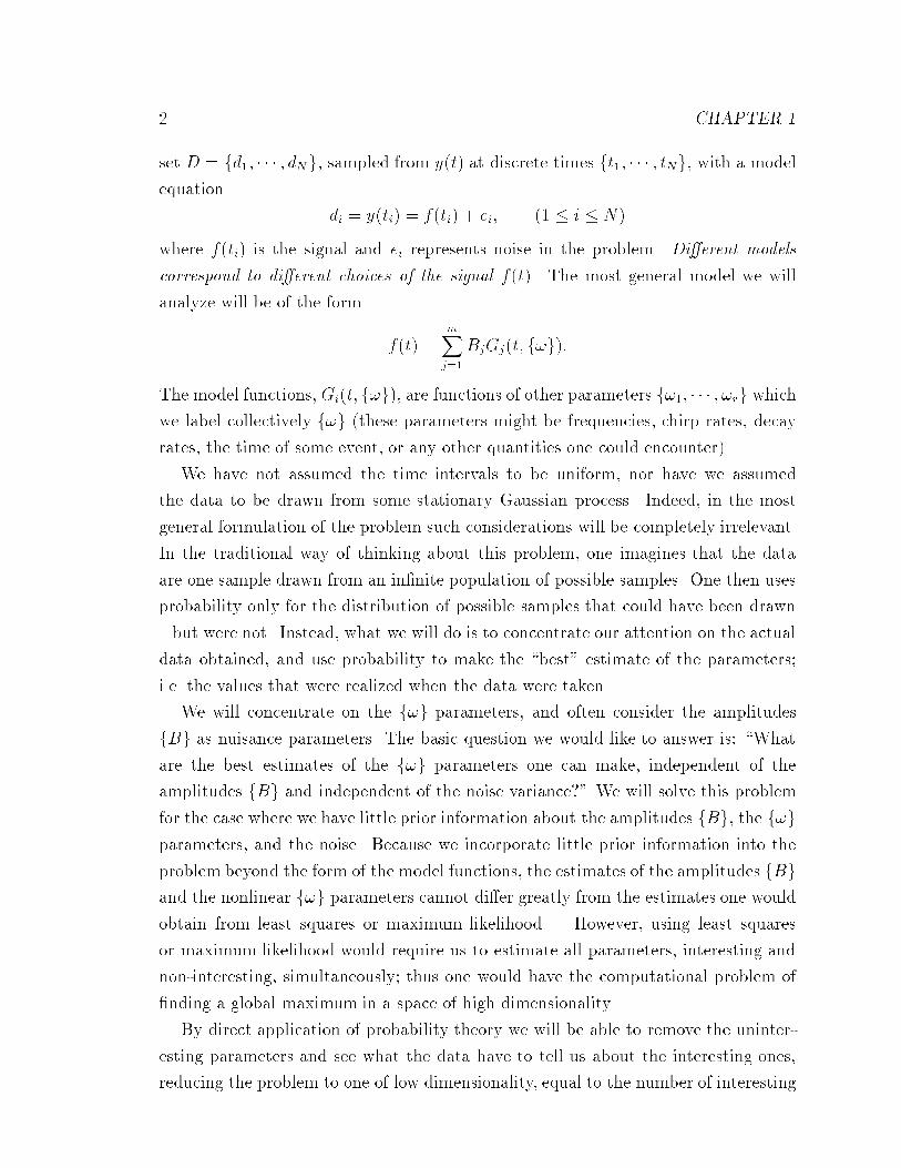
2 CHAPTER 1
set D = fd1; � � � ; dNg, sampled from y(t) at discrete times ft1; � � � ; tNg, with a model
equation
di = y(ti) = f(ti) + ei; (1 � i � N)
where f(ti) is the signal and ei represents noise in the problem. Di�erent models
correspond to di�erent choices of the signal f(t). The most general model we will
analyze will be of the form
f(t) =mXj=1
BjGj(t; f!g):
The model functions, Gi(t; f!g), are functions of other parameters f!1; � � � ; !rg whichwe label collectively f!g (these parameters might be frequencies, chirp rates, decay
rates, the time of some event, or any other quantities one could encounter).
We have not assumed the time intervals to be uniform, nor have we assumed
the data to be drawn from some stationary Gaussian process. Indeed, in the most
general formulation of the problem such considerations will be completely irrelevant.
In the traditional way of thinking about this problem, one imagines that the data
are one sample drawn from an in�nite population of possible samples. One then uses
probability only for the distribution of possible samples that could have been drawn
{ but were not. Instead, what we will do is to concentrate our attention on the actual
data obtained, and use probability to make the \best" estimate of the parameters;
i.e. the values that were realized when the data were taken.
We will concentrate on the f!g parameters, and often consider the amplitudes
fBg as nuisance parameters. The basic question we would like to answer is: \What
are the best estimates of the f!g parameters one can make, independent of the
amplitudes fBg and independent of the noise variance?" We will solve this problem
for the case where we have little prior information about the amplitudes fBg, the f!gparameters, and the noise. Because we incorporate little prior information into the
problem beyond the form of the model functions, the estimates of the amplitudes fBgand the nonlinear f!g parameters cannot di�er greatly from the estimates one would
obtain from least squares or maximum likelihood. However, using least squares
or maximum likelihood would require us to estimate all parameters, interesting and
non-interesting, simultaneously; thus one would have the computational problem of
�nding a global maximum in a space of high dimensionality.
By direct application of probability theory we will be able to remove the uninter-
esting parameters and see what the data have to tell us about the interesting ones,
reducing the problem to one of low dimensionality, equal to the number of interesting
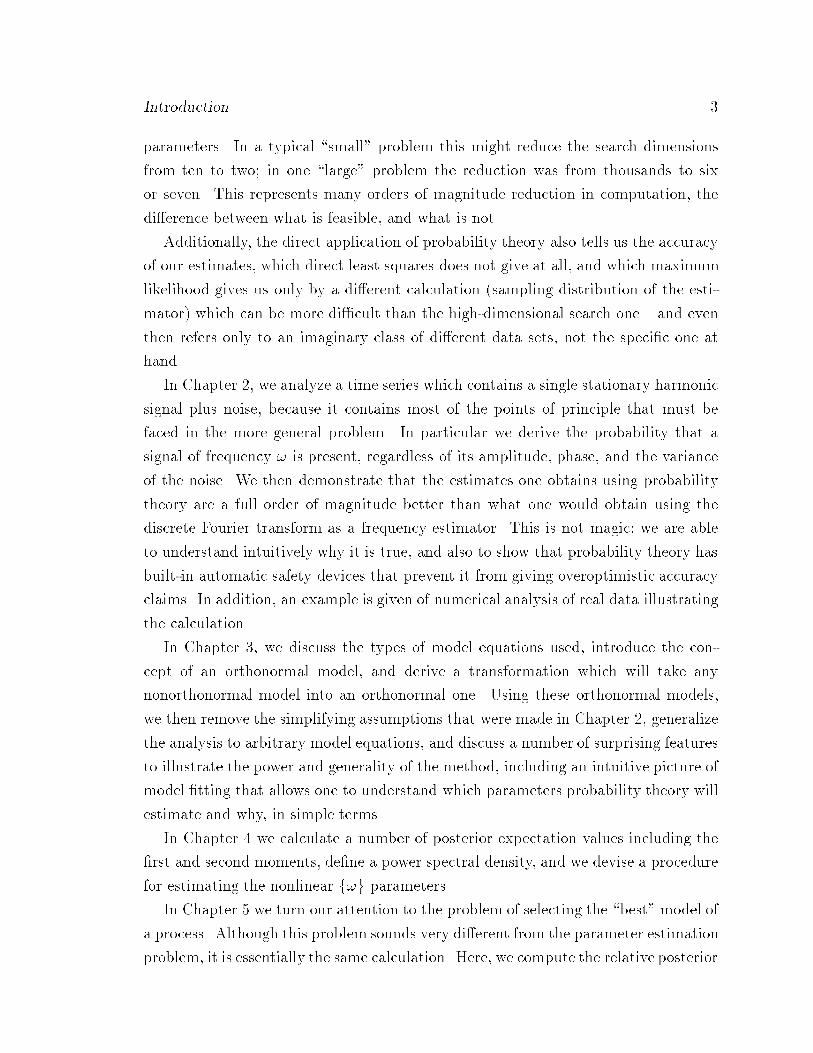
Introduction 3
parameters. In a typical \small" problem this might reduce the search dimensions
from ten to two; in one \large" problem the reduction was from thousands to six
or seven. This represents many orders of magnitude reduction in computation, the
di�erence between what is feasible, and what is not.
Additionally, the direct application of probability theory also tells us the accuracy
of our estimates, which direct least squares does not give at all, and which maximum
likelihood gives us only by a di�erent calculation (sampling distribution of the esti-
mator) which can be more di�cult than the high-dimensional search one { and even
then refers only to an imaginary class of di�erent data sets, not the speci�c one at
hand.
In Chapter 2, we analyze a time series which contains a single stationary harmonic
signal plus noise, because it contains most of the points of principle that must be
faced in the more general problem. In particular we derive the probability that a
signal of frequency ! is present, regardless of its amplitude, phase, and the variance
of the noise. We then demonstrate that the estimates one obtains using probability
theory are a full order of magnitude better than what one would obtain using the
discrete Fourier transform as a frequency estimator. This is not magic; we are able
to understand intuitively why it is true, and also to show that probability theory has
built-in automatic safety devices that prevent it from giving overoptimistic accuracy
claims. In addition, an example is given of numerical analysis of real data illustrating
the calculation.
In Chapter 3, we discuss the types of model equations used, introduce the con-
cept of an orthonormal model, and derive a transformation which will take any
nonorthonormal model into an orthonormal one. Using these orthonormal models,
we then remove the simplifying assumptions that were made in Chapter 2, generalize
the analysis to arbitrary model equations, and discuss a number of surprising features
to illustrate the power and generality of the method, including an intuitive picture of
model �tting that allows one to understand which parameters probability theory will
estimate and why, in simple terms.
In Chapter 4 we calculate a number of posterior expectation values including the
�rst and second moments, de�ne a power spectral density, and we devise a procedure
for estimating the nonlinear f!g parameters.
In Chapter 5 we turn our attention to the problem of selecting the \best" model of
a process. Although this problem sounds very di�erent from the parameter estimation
problem, it is essentially the same calculation. Here, we compute the relative posterior
4 CHAPTER 1
probability of a model: this allows one to select the most probable model based on
how well its parameters are estimated, and how well it �ts the data.
In Chapter 6, we specialize the discussion to spectral estimates and, proceeding
through stages, investigate the one-stationary-frequency problem and explicitly cal-
culate the posterior probability of a simple harmonic frequency independent of its
amplitude, phase and the variance of the noise, without the simplifying assumptions
made in Chapter 2.
At that point we pause brie y to examine some of the assumptions made in the cal-
culation and show that when these assumptions are violated by the data, the answers
one obtains are still correct in a well-de�ned sense, but more conservative in the sense
that the accuracy estimates are wider. We also compare uniform and nonuniform time
sampling and demonstrate that for the single-frequency estimation problem, the use
of nonuniform sampling intervals does not a�ect the ability to estimate a frequency.
However, for apparently randomly sampled time series, aliases e�ectively do not exist.
We then proceed to solve the one-frequency-with-Lorentzian-decay problem and
discuss a number of surprising implications for how decaying signals should be sam-
pled. Next we examine the two stationary frequency problem in some detail, and
demonstrate that (1) the ability to estimate two close frequencies is essentially in-
dependent of the separation as long as that separation is at least one Nyquist step
j!1 � !2j � 2�=N ; and (2) that these frequencies are still resolvable at separations
corresponding to less than one half step, where the discrete Fourier transform shows
only a single peak.
After the two-frequency problem we discuss brie y the multiple nonstationary
frequency estimation problem. In Chapter 3 Eq. (3.17) we derive the joint posterior
probability of multiple stationary or nonstationary frequencies independent of their
amplitude and phase and independent of the noise variance. Here we investigate
some of the implications of these formulas and discuss the techniques and procedures
needed to apply them e�ectively.
In Chapter 7, we apply the theory to a number of real time series, including Wolf's
relative sunspot numbers, some NMR (nuclear magnetic resonance) data containing
multiple close frequencies with decay, and to economic time series which have large
trends. The most spectacular results obtained to date are with NMR data, because
here prior information tells us very accurately what the \true" model must be.
Equally important, particularly in economics, is the way probability theory deals
with trend. Instead of seeking to eliminate the trend from the data (which is known to
Historical Perspective 5
introduce spurious artifacts that distort the information in the data), we seek instead
to eliminate the e�ect of trend from the �nal conclusions, leaving the data intact. This
proves to be not only a safer, but also a more powerful procedure than detrending
the data. Indeed, it is now clear that many published economic time series have been
rendered nearly useless because the data have been detrended or seasonally adjusted
in an irreversible way that destroys information which probability theory could have
extracted from the raw, unmutilated data.
In the last example we investigate the use of multiple measurements and show that
probability theory can continue to obtain the standardpn improvement in parameter
estimates under much wider conditions than averaging. The analyses presented in
Chapter 7 will give the reader a better feel for the types of applications and complex
phenomena which can be investigated easily using Bayesian techniques.
1.1 Historical Perspective
Comprehensive histories of the spectral analysis problem have been given recently
by Robinson [2] and Marple [3]. We sketch here only the part of it that is directly
ancestral to the new work reported here. The problem of determining a frequency
in time sampled data is very old; the �rst astronomers were trying to solve this
problem when they attempted to determine the length of a year or the period of the
moon. Their methods were crude and consisted of little more than trying to locate
the maxima or the nodes of an approximately periodic function. The �rst signi�cant
advance in the frequency estimation problem occurred in the early nineteenth century,
when two separate methods of analyzing the problem came into being: the use of
probability theory, and the use of the Fourier transform.
Probabilistic methods of dealing with the problem were formulated in some gen-
erality by Laplace [4] in the late 18th century, and then applied by Legendre and
Gauss [5] [6] who �rst used (or at least �rst published) the method of least squares
to estimate model parameters in noisy data. In this procedure some idealized model
signal is postulated and the criterion of minimizing the sum of the squares of the
\residuals" (the discrepancies between the model and the data) is used to estimate
the model parameters. In the problem of determining a frequency, the model might
be a single cosine with an amplitude, phase, and frequency, contaminated by noise
with an unknown variance. Generally one is not interested in the amplitude, phase,
6 CHAPTER 1
or noise variance; ideally one would like to formulate the problem in such a way that
only the frequency remains, but this is not possible with direct least squares, which
requires us to �t all the model parameters. The method of least squares may be
di�cult to use in practice; in principle it is well understood. In the case of Gaussian
noise, the least squares estimates are simply the parameter values that maximize the
probability that we would obtain the data, if a model signal was present with those
parameters.
The spectral method of dealing with this problem also has its origin in the early
part of the nineteenth century. The Fourier transform is one of the most powerful tools
in analysis, and its discrete analogue is by de�nition the spectrum of the time sampled
data. How this is related to the spectrum of the original time series is, however,
a nontrivial technical problem whose answer is di�erent in di�erent circumstances.
Using the discrete Fourier transform of the data as an estimate of the \true" spectrum
is, intuitively, a natural thing to do: after all, the discrete Fourier transform is the
spectrum of the noisy time sampled series, and when the noise goes away the discrete
Fourier transform is the spectrum of the sampled \true" series, but calculating the
spectrum of a series and estimating a frequency are very di�erent problems. One of
the things we will attempt to do is to do is to exhibit the exact conditions under
which the discrete Fourier transform is an optimal frequency estimator.
With the introduction (or rather, rediscovery [7], [8], [9]) of the fast Fourier
transform by Cooley and Tukey [10] in 1965 and the development of computers, the
use of the discrete Fourier transform as a frequency and power spectral estimator
has become very commonplace. Like the method of least squares, the use of discrete
Fourier transform as a frequency estimator is well understood. If the data consist of a
signal plus noise, then by linearity the Fourier transform will be the signal transform
plus a noise transform. If one has plenty of data the noise transform will be, usually, a
function of frequency with slowly varying amplitude and rapidly varying phase. If the
peak of the signal transform is larger than the noise transform, the added noise does
not change the location of the peak very much. One can then estimate the frequency
from the location of the peak of the data transform, as intuition suggests.
Unfortunately, this technique does not work well when the signal-to-noise ratio of
the data is small; then we need probability theory. The technique also has problems
when the signal is other than a simple harmonic frequency: then the signal has some
type of structure [for example Lorentzian or Gaussian decay, or chirp: a chirped signal
has the form cos(�+!t+�t2)]. The peak will then be spread out relative to a simple
Historical Perspective 7
harmonic spectrum. This allows the noise to interfere with the parameter estimation
problem much more severely, and probability theory becomes essential. Additionally,
the Fourier transform is not well de�ned when the data are nonuniform in time, even
though the problem of frequency estimation is not essentially changed.
Arthur Schuster [11] introduced the periodogram near the beginning of this cen-
tury, merely as an intuitive ad hoc method of detecting a periodicity and estimating
its frequency. The periodogram is essentially the squared magnitude of the discrete
Fourier transform of the data D � fd1; d2; � � � ; dNg and can be de�ned as
C(!) =1
N
hR(!)2 + I(!)2
i=
1
NjNXj=1
djei!tj j2; (1:1)
where R(!), and I(!) are the real and imaginary parts of the sum [Eqs. (2.4), and
(2.5) below], and N is the total number of data points. The periodogram remains
well de�ned when the frequency ! is allowed to vary continuously or when the data
are nonuniform. This avoids one of the potential drawbacks of using this method but
does not aid in the frequency estimation problem when the signal is not stationary.
Although Schuster himself had very little success with it, more recent experience has
shown that regardless of its drawbacks, indeed the discrete Fourier transform or the
periodogram does yield useful frequency estimates under a wide variety of conditions.
Like least squares, Fourier analysis alone does not give an indication of the accuracy
of the estimates of spectral density, although the width of a sharp peak is suggestive
of the accuracy of determination of the position of a very sharp line.
In the 160 years since the introduction of the spectral and probability theory
methods no particular connection between them had been noted, yet each of these
methods seems to function well in some conditions. That these methods could be very
closely related (from some viewpoints essentially the same) was shown when Jaynes
[12] derived the periodogram directly from the principles of probability theory and
demonstrated it to be, a \su�cient statistic" for inferences about a single station-
ary frequency or \signal" in a time sampled data set, when a Gaussian probability
distribution is assigned for the noise. That is, starting with the same probability dis-
tribution for the noise that had been used for maximum likelihood or least squares,
the periodogram was shown to be the only function of the data needed to make es-
timates of the frequency; i.e. it summarizes all the information in the data that is
relevant to the problem.
In this work we will continue the analysis started by Jaynes and show that when
the noise variance �2 is known, the conditional posterior probability density of a

8 CHAPTER 1
frequency ! given the data D, the noise variance �2, and the prior information I is
simply related to the periodogram:
P (!jD;�; I) / exp
(C(!)
�2
): (1:2)
Thus, we will have demonstrated the relation between the two techniques. Because
the periodogram, and therefore the Fourier transform, will have been derived from
the principles of probability theory we will be able to see more clearly under what
conditions the discrete Fourier transform of the data is a valid frequency estimator
and the proper way to extract optimum estimates from it. Also, from (1.2) we will
be able to assess the accuracy of our estimates, which neither least squares, Fourier
analysis, nor maximum likelihood give directly.
The term \spectral analysis" has been used in the past to denote a wider class of
problems than we shall consider here; often, one has taken the view that the entire
time series is a \stochastic process" with an intrinsically continuous spectrum, which
we seek to infer. This appears to have been the viewpoint underlying the work of
Schuster, and of Blackman-Tukey noted in the following sections. For an account of
the large volume of literature on this version of the spectral estimation problem, we
refer the reader to Marple [3].
The present work is concerned with what Marple calls the \parameter estimation
method". Recent experience has taught us that this is usually a more realistic way
of looking at current applications; and that when the parameter estimation approach
is based on a correct model it can achieve far better results than can a \stochastic"
approach, because it incorporates cogent prior information into the calculation. In
addition, the parameter estimation approach proves to be more exible in ways that
are important in applications, adapting itself easily to such complicating features as
chirp, decay, or trend.
1.2 Method of Calculation
The basic reasoning used in this work will be a straightforward application of
Bayes' theorem: denoting by P (AjB) the conditional probability that proposition A
is true, given that proposition B is true, Bayes' theorem is
P (HjD; I) = P (HjI)P (DjH; I)P (DjI) : (1:3)
Method of Calculation 9
It is nothing but the probabilistic statement of an almost trivial fact: Aristotelian
logic is commutative. That is, the propositions
HD = \ Both H and D are true"
DH = \Both D and H are true"
say the same thing, so they must have the same truth value in logic and the same
probability, whatever our information about them. In the product rule of probability
theory, we may then interchange H and D
P (H;DjI) = P (DjI)P (HjD; I) = P (HjI)P (DjH; I)
which is Bayes' theorem. In our problems, H is any hypothesis to be tested, D is
the data, and I is the prior information. In the terminology of the current statisti-
cal literature, P (HjD; I) is called the posterior probability of the hypothesis, given
the data and the prior information. This is what we would like to compute for sev-
eral di�erent hypotheses concerning what systematic \signal" is present in our data.
Bayes' theorem tells us that to compute it we must have three terms: P (HjI) is theprior probability of the hypothesis (given only our prior information), P (DjI) is theprior probability of the data (this term will always be absorbed into a normalization
constant and will not change the conclusions within the context of a given model,
although it does a�ect the relative probabilities of di�erent models) and P (DjH; I) iscalled the direct probability of the data, given the hypothesis and the prior informa-
tion. The direct probability is called the \sampling distribution" when the hypothesis
is held constant and one considers di�erent sets of data, and it is called the \likelihood
function" when the data are held constant and one varies the hypothesis. Often, a
prior probability distribution is called simply a \prior".
In a speci�c Bayesian probability calculation, we need to \de�ne our model"; i.e.
to enumerate the set fH1;H2; � � �g of hypotheses concerning the systematic signal in
the model, that is to be tested by the calculation. A serious weakness of all Fourier
transform methods is that they do not consider this aspect of the problem. In the
widely used Blackman-Tukey [13] method of spectrum analysis, for example, there
is no mention of any model or any systematic signal at all. In the problems we are
considering, speci�cation of a de�nite model (i.e. stating just what prior information
we have about the phenomenon being observed) is essential; the information we can
extract from the data depends crucially on which model we analyze.

10 CHAPTER 1
In our problems, therefore, the Blackman-Tukeymethod, which does not even have
the concept of a signal, much less a signal-to-noise ratio, would be inappropriate.
Bayesian analysis based on a good model can achieve orders of magnitude better
sensitivity and resolution. Indeed, one of our main new results is the very great
improvement in resolution that can be achieved by replacing an unrealistic model by
a realistic one.
In the most general model we will analyze, the hypothesis H will be of the form
H � \f(t) =mXj=1
BjGj(t; f!g)"
where f(t) is some analytic representation of the time series, Gj(t; f!g) is one par-ticular model function (for example a sinusoid or trend), Bj is the amplitude with
which Gj enters the model, and f!g is a set of frequencies, decay rates, chirp rates,
trend rate, or any other parameters of interest.
In the problem we are considering we focus our attention on the f!g parameters.
Although we will calculate the expectation value of the amplitudes fBg we will notgenerally be interested in them. We will seek to formulate the posterior probability
density P (f!gjD; I) independently of the amplitudes fBg.The principles of probability theory uniquely determine how this is to be done.
Suppose ! is a parameter of interest, and B is a \nuisance parameter" that we do
not, at least at the moment, need to know. What we want is P (!jD; I), the posteriorprobability (density) of !. This may be calculated as follows: �rst calculate the joint
posterior probability density of ! and B by Bayes' theorem:
P (!;BjD; I) = P (!;BjI)P (Dj!;B; I)P (DjI)
and then integrate out B, obtaining the marginal posterior probability density for !:
P (!jD; I) =ZdBP (!;BjD; I)
which expresses what the data and prior information have to tell us about !, regard-
less of the value of B.
Although integration over the nuisance parameters may look a little strange at �rst
glance, it is easily demonstrated to be a straightforward application of the sum rule of
probability theory: the probability that one of several mutually exclusive propositions
is true, is the sum of their separate probabilities. Suppose for simplicity that B is a
discrete variable taking on the values fB1; � � � ; Bng and we know that when the data
Method of Calculation 11
were taken only one value of B was realized; but we do not know which value. We
can compute P (!;Pn
i=1BijD; I) where the symbol \+" or \P" inside a probability
symbol means the Boolean \or" operation [read this as the probability of (! and B1)
or (! and B2) � � �]. Using the sum rule this probability may be written
P (!;B1 +nXi=2
BijD; I) = P (!;B1jD; I)
+ P (!;nXi=2
BijD; I)[1� P (!;B1jnXi=2
BiD; I)]:
The last term P (!;B1jPn
i=2BiD; I) is zero: only one value of B could be realized.
We have
P (!;B1 +nXi=2
BijD; I) = P (!;B1jD; I) + P (!;nXi=2
BijD; I)
and repeated application of the sum rule gives
P (!;nXi=1
BijD; I) =nXi=1
P (!;BijD; I):
When the values of B are continuous the sums go into integrals and one has
P (!jD; I) =ZdBP (!;BjD; I); (1:4)
the given rule. The term on the left is called the marginal posterior probability density
function of !, and it takes into account all possible values of B regardless of which
actual value was realized. We have dropped the reference to B speci�cally because
this distribution no longer depends on one speci�c value of B; it depends rather on
all of them.
We discuss these points further in Appendices A, B, and C where we show that
this procedure is similar to, but superior to, the common practice of estimating the
parameter B from the data and then constraining B to that estimate.
In the following chapter we consider the simplest nontrivial spectral estimation
model
f(t) = B1 cos!t+B2 sin!t
and analyze it in some depth to show some elementary but important points of prin-
ciple in the technique of using probability theory with nuisance parameters and \un-
informative" priors.

12 CHAPTER 1

Chapter 2
SINGLE STATIONARY
SINUSOID PLUS NOISE
2.1 The Model
We begin the analysis by constructing the direct probability, P (DjH; I). We think
of this as the likelihood of the parameters, because it is its dependence on the model
parameters which concerns us here. The time series y(t) we are considering is postu-
lated to contain a single stationary harmonic signal f(t) plus noise e(t). The basic
model is always: we have recorded a discrete data set D = fd1; � � � ; dNg; sampled
from y(t) at discrete times ft1; � � � ; tNg; with a model equation
di = y(ti) = f(ti) + ei; (1 � i � N):
As already noted, di�erent models correspond to di�erent choices of the signal f(t).
We repeat the analysis originally done by Jaynes [12] using a di�erent, but equivalent,
set of model functions. We repeat this analysis for three reasons: �rst, by using a
di�erent formulation of the problem we can see how to generalize to multiple fre-
quencies and more complex models; second, to introduce a di�erent prior probability
for the amplitudes, which simpli�es the calculation but has almost no e�ect on the
�nal result; and third, to introduce and discuss the calculation techniques without
the complex model functions confusing the issues.
The model for a simple harmonic frequency may be written
f(t) = B1 cos(!t) +B2 sin(!t) (2:1)
which has three parameters (B1; B2; !) that may be estimated from the data. The
13
14 CHAPTER 2
model used by Jaynes [12] was the same, but expressed in polar coordinates:
f(t) = B cos(!t+ �)
B =qB2
1 +B22
tan � = �B2
B1
dB1dB2d! = BdBd�d!:
It is the factor B in the volume elements which is treated di�erently in the two
calculations. Jaynes used a prior probability that initially considered equal intervals
of � and B to be equally likely, while we shall use a prior that initially considers equal
intervals of B1 and B2 to be equally likely.
Of course, neither choice fully expresses all the prior knowledge we are likely to
have in a real problem. This means that the results we �nd are conservative, and
in a case where we have quite speci�c prior information about the parameters, we
would be able to do somewhat better than in the following calculation. However,
the di�erences arising from di�erent prior probabilities are small provided we have
a reasonable amount of data. For a detailed discussion and derivation of the prior
probabilities used in this chapter, see Appendix A. In addition, in Appendix D
we show explicitly that the prior used by Jaynes is more conservative for frequency
estimation than the uniform prior we use, but when the signal-to-noise ratio is large
the e�ect of this uninformative prior is completely negligible.
2.2 The Likelihood Function
To construct the likelihood we take the di�erence between the model function, or
\signal", and the data. If we knew the true signal, then this di�erence would be just
the noise. Then if we knew the probability of the noise we could compute the direct
probability or likelihood. We wish to assign a noise prior probability density which
is consistent with the available information about the noise. The prior should be as
uninformative as possible to prevent us from \seeing" things in the data which are
not there.
To derive the prior probability for the noise is a problem that can be approached
in various ways. Perhaps the most general one is to view it as a simple application
of the principle of maximum entropy. Let P (ejI) stand for the probability that the

The Likelihood Function 15
noise has value \e" given the prior information I. Then, assuming the second moment
of the noise (i.e. the noise power) is known, the entropy functional which must be
maximized is given by
�Z +1
�1P (ejI) logP (ejI)de� �
Z +1
�1e2P (ejI)de� �
Z +1
�1P (ejI)de
where � is the Lagrange multiplier associated with the second moment, and � is the
multiplier for normalization. The solution to this standard maximization problem is
P (ej�; I) = (�=�)12 exp
n��e2
o:
Adopting the notation � = (2�2)�1, where �2 is the second moment, assumed known,
we have
P (ej�; I) = 1p2��2
exp
(� e2
2�2
):
This is a Gaussian distribution, and when � is taken as the RMS noise level, it is the
least informative prior probability density for the noise that is consistent with the
given second moment. By least informative we mean that: if any of our assumptions
had been di�erent and we used that information in maximum entropy to derive a new
prior probability for the noise, then for a given �, that new probability density would
be less spread out, thus our accuracy estimates would be narrowed. Thus, in the
calculations below, we will be claiming less accuracy than would be justi�ed had we
included those additional e�ects in deriving the prior probability for the noise. The
point is discussed further in Chapter 5. In Chapter 6 we demonstrate (numerically)
the e�ects of violating the assumptions that will go into the calculation. All of these
\conservative" features are safety devices which make it impossible for the theory to
mislead us by giving overoptimistic results.
Having the prior probability for the noise, and adopting the notation: ei is the noise
at time ti, we apply the product rule of probability theory to obtain the probability
that we would obtain a set of noise values fe1; � � � ; eNg: supposing the ei independentin the sense that P (eijej; �; I) = P (eij�; I) this is given by
P (e1; � � � ; eN j�; I) /NYi=1
"1p2��2
exp(� e2i2�2
)
#;
in which the independence of di�erent ei is also a safety device to maintain the conser-
vative aspect. But if we have de�nite prior evidence of dependence, i.e. correlations,
it is a simple computational detail to take it into account as noted later.
16 CHAPTER 2
Other rationales for this choice exist in other situations. For example, if the noise is
known to be the result of many small independent e�ects, the central limit theorem
of probability theory leads to the Gaussian form independently of the �ne details,
even if the second moment is not known. For a detailed discussion of why and when
a Gaussian distribution should be used for the noise probability, see the original
paper by Jaynes [12]. Additionally, the book of Jaynes' collected papers contains a
discussion of the principle of maximum entropy and much more [14].
If we have the true model, the di�erence between the data di and the model
fi is just the noise. Then the direct probability that we should obtain the data
D = fd1 � � � dNg, given the parameters, is proportional to the likelihood function:
P (DjB1; B2; !; �; I) / L(B1; B2; !; �) =NYi=1
��1 expf� 1
2�2[di � f(ti)]
2g
L(B1; B2; !; �) = ��N � expf � 1
2�2
NXi=1
[di � f(ti)]2g: (2:2)
The usual way to proceed is to �t the sum in the exponent. Finding the parameter
values which minimize this sum is called \least squares". The equivalent procedure
(in this case) of �nding parameter values that maximize L(B1; B2; !; �) is called
\maximum likelihood". The maximum likelihood procedure is more general than
least squares: it has theoretical justi�cation when the likelihood is not Gaussian. The
departure of Jaynes was to use (2.2) in Bayes' theorem (1.3), and then to remove the
phase and amplitude from further consideration by integration over these parameters.
In doing this preliminary calculation we will make a number of simplifying as-
sumptions, then in Chapter 3 correct them by solving a much more general problem
exactly. For now we insert the model (2.1) into the likelihood (2.2) and expand the
exponent to obtain:
L(B1; B2; !; �) / ��N exp��NQ
2�2
�(2:3)
where
Q � d2 � 2
N[B1R(!) +B2I(!)] +
1
2(B2
1 +B22);
and
R(!) =NXi=1
di cos(!ti) (2:4)
I(!) =NXi=1
di sin(!ti) (2:5)

The Likelihood Function 17
are the functions introduced in (1.1), and
d2 =1
N
NXi=1
d2i
is the observed mean-square data value. In this preliminary discussion we assumed
the data have zero mean value (any nonzero average value has been subtracted from
the data), and we simpli�ed the quadratic term as follows:
NXi=1
f(ti)2 = B2
1
NXi=1
cos2 !ti +B22
NXi=1
sin2 !ti + 2B1B2
NXi=1
cos(!ti) sin(!ti);
withNXi=1
cos2 !ti =N
2+1
2
NXi=1
cos 2!ti 'N
2;
NXi=1
sin2 !ti =N
2� 1
2
NXi=1
cos 2!ti 'N
2;
NXi=1
cos(!ti) sin(!ti) =1
2
NXi=1
sin(2!ti)�N
2
so the quadratic term is approximately
NXi=1
f(ti)2 � N
2
�B2
1 +B22
�:
The neglected terms are of order one, and small provided N � 1 (except in the
special case !tN � 1). We will assume, for now, that the data contain no evidence
of a low frequency.
The cross term,PN
i=1 cos(!ti) sin(!ti), is at most of the same order as the terms
we just ignored; therefore, this term is also ignored. The assumption that this cross
term is zero is equivalent to assuming the sine and cosine functions are orthogonal
on the discrete time sampled set. Indeed, this is the actual case for uniformly spaced
time intervals; however, even without uniform spacing this is a good approximation
provided N is large. The assumption that the cross terms are zero by orthogonality
will prove to be the key to generalizing this problem to more complex models, and in
Chapter 3 the assumptions that we are making now will become exact by a change
of variables.
18 CHAPTER 2
2.3 Elimination of Nuisance Parameters
In a harmonic analysis one is primarily interested in the frequency !. Then if
the amplitude, phase, and the variance of the noise are unknown, they are nuisance
parameters. We gave the general procedure for dealing with nuisance parameters in
Chapter 1. To apply that rule we must integrate the posterior probability density
with respect to B1, B2, and also � if the noise variance is unknown.
If we had prior information about the nuisance parameters (such as: they had to
be positive, they could not exceed an upper limit, or we had independently measured
values for them) then here would be the place to incorporate that information into the
calculation. We illustrate the e�ects of integrating over a nuisance parameter, as well
as the use of prior information in, Appendices B and C and explicitly calculate the
expectation values of B1 and B2 when a prior measurement is available. At present we
assume no prior information about the amplitudesB1 and B2 and assign them a prior
probability which indicates \complete ignorance of a location parameter". This prior
is a uniform, at, prior density; it is called an improper prior probability because it
is not normalizable. In principle, we should approach an improper prior as the limit
of a sequence of proper priors. The point is discussed further in Appendices A and B.
However, in this problem there are no di�culties with the use of the uniform prior
because the Gaussian cuto� in the likelihood function ensures convergence in (2.3).
Upon multiplying the likelihood (2.3) by the uniform prior and integrating with
respect to B1 and B2 one obtains the joint quasi-likelihood of ! and �:
L(!; �) / ��N+2 � exp�� N
2�2[d2 � 2C(!)=N ]
�(2:6)
where C(!), the Schuster periodogram de�ned in (1.1), has appeared in a very natural
and unavoidable way. If one knows the variance �2 from some independent source
and has no additional prior information about !, then the problem is completed. The
posterior probability density for ! is given by
P (!jD;�; I) / exp
(C(!)
�2
): (2:7)
Because we have assumed little prior information about B1, B2, ! and have made con-
servative assumptions about the noise; this probability density will yield conservative
estimates of !. By this we mean, as before, that if we had more prior information,
we could exploit it to obtain still better results. We will illustrate this point further
Elimination of Nuisance Parameters 19
in Chapter 5 and show that when the data have characteristics which di�er from our
assumptions, Eq. (2.7) will always make a conservative estimates of the frequency !.
Thus the assumptions we are making act as safeguards to protect us from seeing
things in the data that are not really there. We place such great stress on this point
because we shall presently obtain some surprisingly sharp estimates.
The above analysis is valid whenever the noise variance (or power) is known.
Frequently one has no independent prior knowledge of the noise. The noise variance
�2 then becomes a nuisance parameter. We eliminate it in much the same way as the
amplitudes were eliminated. Now � is restricted to positive values and additionally
it is a scale parameter. The prior which indicates \complete ignorance" of a scale is
the Je�reys prior 1=� [15]. Multiplying Eq. (2.6) by the Je�reys prior and integrating
over all positive values gives
P (!jD; I) /�1� 2C(!)
Nd2
� 2�N2
: (2:8)
This is called a \Student t-distribution" for historical reasons, although it is expressed
here in very nonstandard notation. In our case it is the posterior probability density
that a stationary harmonic frequency ! is present in the data when we have no prior
information about �.
These simple results, Eqs. (2.7) and (2.8), show why the discrete Fourier transform
tends to peak at the location of a frequency when the data are noisy. Namely, the
discrete Fourier transform is directly related to the probability that a single harmonic
frequency is present in the data, even when the noise level is unknown. Additionally,
zero padding a time series (i.e. adding zeros at its end to make a longer series) and then
taking the Fast Fourier transform of the padded series, is equivalent to calculating the
Schuster periodogram at smaller frequency intervals. If the signal one is analyzing is
a simple harmonic frequency plus noise, then the maximum of the periodogram will
be the \best" estimate of the frequency that we can make in the absence of additional
prior information about it.
We now see the discrete Fourier transform and the Schuster periodogram in a
entirely new light: the highest peak in the discrete Fourier transform is an optimal
frequency estimator for a data set which contains a single harmonic frequency in
the presence of Gaussian white noise. Stated more carefully, the discrete Fourier

20 CHAPTER 2
transform will give optimal frequency estimates if six conditions are met:
1. The number of data values N is large,2. There is no constant component in the data,3. There is no evidence of a low frequency,4. The data contain only one frequency,5. The frequency must be stationary
(i.e. the amplitude and phase are constant),6. The noise is white.
If any of these six conditions is not met, the discrete Fourier transform may give
misleading or simply incorrect results in light of the more realistic models. Not
because the discrete Fourier transform is wrong, but because it is answering what
we should regard as the wrong question. The discrete Fourier transform will always
interpret the data in terms of a single harmonic frequency model! In Chapter 6 we
illustrate the e�ects of violating one or more of these assumptions and demonstrate
that when they are violated the estimated parameters are always less certain than
when these conditions are met.
2.4 Resolving Power
When the six conditions are met, just how accurately can the frequency be es-
timated? This question is easily answered; we do this by approximating (2.7) by
a Gaussian and then making the (mean) � (standard deviation) estimates of the
frequency !. Expanding C(!) about the maximum ! we have
C(!) = C(!)� b
2(! � !)2 + � � �
where
b � �C 00(!) > 0: (2:9)
The Gaussian approximation is
P (!jD;�; I) '"2b
��2
# 12
exp
(�b(! � !)2
2�2
)
from which we would make the (mean) � (standard deviation) estimate of the fre-
quency
!est = ! � �pb:
Resolving Power 21
The accuracy depends on the curvature of C(!) at its peak, not on the height of
C(!). For example, if the data are composed of a single sine wave plus noise e(t) of
standard deviation �
dt = B1 cos(!t) + et
then as found by Jaynes [12]:
C(!max) 'NB2
1
4
b ' B21N
3
48
(!)est = ! � �
jB1jq48=N3 (2:10)
which indicates, as intuition would lead us to expect, that the accuracy depends on
the signal-to-noise ratio, and quite strongly on how much data we have.
The height of the posterior probability density increases like the exponential of
NB21=4�
2 while the error estimates depend on the exponential of N3B21=96�
2. If one
has a choice between doubling the amount of data N ! 2N , or doubling the signal-
to-noise ratio B1=�! 2B1=�, always double the amount of data if you have detected
the signal, and always double the signal-to-noise ratio if you have no strong evidence
of a signal.
If we have su�cient signal-to-noise ratio for the posterior probability density
expfNB21=4�
2g to have a peak well above the noise, doubling the amount of data,
N ! 2N will double the height of the periodogram giving expfNB21=4�
2g times more
evidence of a frequency while the error will go down likep8. On the other hand, if the
signal-to-noise ratio is so low that expfNB21=4�
2g has no clear peak above the noise,
then doubling the signal-to-noise ratio B21=�
2 ! 4B21=�
2 will give expf3NB21=4�
2gtimes more evidence for a frequency, while the error goes down by 2. The trade
o� is clear: if you have su�cient signal-to-noise for signal detection more data are
important for resolution; otherwise more signal-to-noise will detect the signal with
less data.
We can further compare these results with experience, but �rst note that we are
using dimensionless units, since we took the data sampling interval to be 1. Convert-
ing to ordinary physical units, let the sampling interval be �t seconds, and denote
by f the frequency in Hz. Then the total number of cycles in our data record is
!(N � 1)
2�= (N � 1)f�t = fT
22 CHAPTER 2
where T = (N � 1)�t seconds is the duration of our data run. So the conversion of
dimensionless ! to f in physical units is
f =!
2��tHz:
The frequency estimate (2.10) becomes
fest = f � �f Hz
where now, not distinguishing between N and (N � 1),
�f =�
2�B1T
q48=N =
1:1�
B1TpN
Hz: (2:11)
Comparing this with (2.10) we now see that to improve the accuracy of the estimate
the two most important factors are how long we sample (the T dependence) and the
signal-to-noise ratio. We could double the number of data values in one of two ways,
by doubling the total sampling time or by doubling the sampling rate. However, (2.11)
clearly indicates that doubling the sampling time is to be preferred. This indicates
that data values near the beginning and end of a record are most important for
frequency estimation, in agreement with intuitive common sense.
Let us take a speci�c example: if we have an RMS signal-to-noise ratio (i.e. ratio
of RMS signal to RMS noise � S/N) of S/N = B1=p2� = 1, and we take data every
�t = 10�3 sec. for T = 1 second, thus getting N = 1000 data points, the theoretical
accuracy for determining the frequency of a single steady sinusoid is
�f =1:1p2000
= 0:025 Hz (2:12)
while the Nyquist frequency for the onset of aliasing is fN = (2�t)�1 = 500Hz, greater
by a factor of 20,000.
To some, this result will be quite startling. Indeed, had we considered the peri-
odogram itself to be a spectrum estimator, we would have calculated instead the width
of its central peak. A noiseless sinusoid of frequency ! would have a periodogram
proportional to
C(!) / sin2fN(! � !)=2gsin2f(! � !)=2g
thus the half-width at half amplitude is given by jN(!�!)=2j = �=4 or �! = �=2N .
Converting to physical units, the periodogram will have a width of about
�f =1
4N�t=
1
4T= 0:25 Hz (2:13)
Resolving Power 23
just ten times greater than the value (2.12) indicated by probability theory. This
factor of ten is the amount of narrowing produced by the exponential peaking of the
periodogram in (2.7), even for unit signal-to-noise ratio.
But some would consider even the result (2.13) to be a little overoptimistic. The
famous Rayleigh criterion [16] for resolving power of an optical instrument supposes
that the minimum resolvable frequency di�erence corresponds to the peak of the
periodogram of one sinusoid coming at the �rst zero of the periodogram of the second.
This is twice (2.13):
�fRayleigh =1
2T= 0:5 Hz: (2:14)
There is a widely believed \folk-theorem" among theoreticians without laboratory
experience, which seems to confuse the Rayleigh limit with the Heisenberg uncertainty
principle, and holds that (2.14) is a fundamental irreducible limit of resolution. Of
course there is no such theorem, and workers in high resolution NMR have been
routinely determining line positions to an accuracy that surpasses the Rayleigh limit
by an order of magnitude, for thirty years.
The misconception is perhaps strengthened by the curious coincidence that (2.14)
is also the minimum half-width that can be achieved by a Blackman-Tukey spec-
trum analysis [13] (even at in�nite signal-to-noise ratio) because the \Hanning win-
dow" tapering function that is applied to the data to suppress side-lobes (the sec-
ondary maxima of [sin(x)=x]2) just doubles the width of the periodogram. Since
the Blackman-Tukey method has been used widely by economists, oceanographers,
geophysicists, and engineers for many years, it has taken on the appearance of an
optimum procedure.
According to E.T. Jaynes, Tukey himself acknowledged [17] that his method fails
to give optimum resolution, but held this to be of no importance because \real time
series do not have sharp lines." Nevertheless, this misconception is so strongly held
that there have been attacks on the claims of Bayesian/MaximumEntropy spectrum
analysts to be able to achieve results like (2.12) when the assumed conditions are
met. Some have tried to put such results in the same category with circle squaring
and perpetual motion machines. Therefore we want to digress to explain in very
elementary physical terms why it is the Bayesian result (2.11) that does correspond
to what a skilled experimentalist can achieve.
Suppose �rst that our only data analysis tool is our own eyes looking at a plot of
the raw data of duration T = 1 sec., and that the unknown frequency f in (2.12) is
100Hz. Now anyone who has looked at a record of a sinusoid and equal amplitude
24 CHAPTER 2
wide-band noise, knows that the cycles are quite visible to the eye. One can count
the total number of cycles in the record con�dently (using interpolation to help us
over the doubtful regions) and will feel quite sure that the count is not in error by
even one cycle. Therefore by raw eyeballing of the data and counting the cycles, one
can achieve an accuracy of
�f ' 1
T= 1 Hz:
But in fact, if one draws the sine wave that seems to �t the data best, he can make a
quite reliable estimate of how many quarter-cycles were in the data, and thus achieve
�f ' 1
4T= 0:25 Hz
corresponding just to the periodogram width (2.13).
Then the use of probability theory needs to surpass the naked eye by another
factor of ten to achieve the Bayesian width (2.12). What probability theory does
is essentially to average out the noise in a way that the naked eye cannot do. If we
repeat some measurementN times, any randomly varying component of the data will
be suppressed relative to the systematic component by a factor of N� 12 , the standard
rule.
In the case considered, we assumed N = 1000 data points. If they were all in-
dependent measurements of the same quantity with the same accuracy, this would
suppress the noise by about a factor of 30. But in our case not all measurements
are equally cogent for estimating the frequency. Data points in the middle of the
record contribute very little to the result; only data points near the ends are highly
relevant for determining the frequency, so the e�ective number of observations is less
than 1000. The probability analysis leading to (2.12) indicates that the \e�ective
number of observations" is only about N=10 = 100; thus the Bayesian width (2.12)
that results from the exponential peaking of the periodogram now appears to be, if
anything, somewhat conservative.
Indeed, that is what Bayesian analysis always does when we use smooth, uninfor-
mative priors for the parameters, because then probability theory makes allowance
for all possible values that they might have. As noted before, if we had any cogent
prior information about ! and expressed it in a narrower prior, we would be led to
still better results; but they would not be much better unless the prior range became
comparable to the width of the likelihood L(!).
2.5. THE POWER SPECTRAL DENSITY P 25
2.5 The Power Spectral Density p
The usual way the result from a spectral analysis is displayed is in the form of a
power spectral density (i.e. power per unit frequency). In Fourier transform spec-
troscopy this is typically taken as the squared magnitude of the discrete Fourier
transform of the data. We would like to express the results of the present calcula-
tion in a similar manner to facilitate comparisons between these techniques, although
strictly speaking there is no exact correspondence between a spectral density de�ned
with reference to a stochastic model and one that pertains to a parameter estimation
model.
We begin by de�ning what we mean by the \estimated spectrum," since several
quite di�erent meanings of the term can be found in the literature. De�ne p(!)d! as
the expectation, over the joint posterior probability distribution for all the parameters,
of the energy carried by the signal (not the noise) in frequency range d!, during our
observation time tN�t1. ThenRp(!)d! over some frequency range is the expectation
of the total energy carried by the signal in that frequency range. The total energy E
carried by the signal in our model is
E =Z tN
t1
f(t)2dt � T
2
�B2
1 +B22
�
and its expectation is given by
p(!) =T
2hB2
1 +B22i;
but N = T=�t, where �t is the sampling time which in dimensionless units is one.
The power spectral density is
p(!) =N
2
ZdB1dB2(B
21 +B2
2)P (!;B1; B2jD;�; I):
Performing the integrals over B1 and B2 we obtain
p(!) = 2h�2 + C(!)
iP (!jD;�; I): (2:15)
We see now that the peak of the periodogram is indicative of the total energy carried
by the signal. The additional term 2�2 is not di�cult to explain; but we delay
that explanation until after we have derived these results for the general theory (see
page 52).
26 CHAPTER 2
If the noise variance is assumed known, (2.15) becomes
p(!) = 2h�2 + C(!)
i exp fC(!)=�2gZd! exp
nC(!)=�2
o: (2:16)
Probability theory will handle those secondary maxima (side lobes) that occur in the
periodogram by assigning them negligible weight.
This is easily seen by considering the same example discussed earlier. Take d(t) =
B1 cos(!t) sampled on a uniform grid; then when ! ' !
C(!) ' B21
4N
"sinN(! � !)=2
(! � !)=2
#2
and C 00 is
C 00 � b ' B21N
3
24
and p(!) is approximately
p(!) ' 2
"�2 +
4B21 sin
2N(! � !)=2
(! � !)2
# "B2
1N3
24��2
# 12
exp
(�B
21N
3
48�2(! � !)2
):
Unless the signal-to-noise ratio B1=�p2 is very small, this is very nearly a delta
function.
If we take B1 =p2� = 1, and N = 1000 data values, then
p(!) ' 2
"1 + 4
sin2 1000(! � !)=2
(! � !)2
#[5150] expf�4� 107(! � !)2g:
This reaches a maximumvalue of 1011 at ! = ! and has dropped to 1
2this value when
!�! has changed by only 0:0001; this function is indeed a good approximation to a
delta function and (2.16) may be approximated by:
p(!) 'h�2 + C(!)
i[�(! � !) + �(! + !)]
for most purposes. But for the term �2, the peak of the periodogram is, in our model,
nearly the total energy carried by the signal. It is not an indication of the spectral
density as Schuster [11] supposed it to be for a stochastic model. In the present
model, the periodogram of the data is not even approximately the spectral energy
density of the signal.

2.6. WOLF'S RELATIVE SUNSPOT NUMBERS 27
2.6 Wolf's Relative Sunspot Numbers
Wolf's relative sunspot numbers are, perhaps, the most analyzed set of data in all
of spectrum analysis. As Marple [3] explains in more detail, these numbers (de�ned
as: W = k[10g + f ], where g is the number of sunspot groups, f is the number of
individual sunspots, and k is used to reduce di�erent telescopes to a common scale)
have been collected on a yearly basis since 1700, and on a monthly basis since 1748
[18]. The exact physical mechanism which generates the sunspots is unknown, and
no complete theory exists. Di�erent analyses of these numbers have been published
more or less regularly since their tabulation began. Here we will analyze the sunspot
numbers with a number of di�erent models including the simple harmonic analysis
just completed, even though we know this analysis is too simple to be realistic for
these numbers.
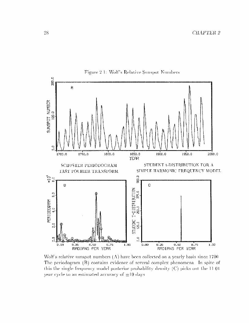
We have plotted the time series from 1700 to 1985 in Fig. 2.1(A). A cursory
examination of this time series does indeed show a cyclic variation with a period
of about 11 years. The square of the discrete Fourier transform is a continuous
function of frequency and is proportional to the Schuster periodogram of the data
Fig. 2.1(B), continuous curve. The frequencies could be restricted to the Nyquist [19]
[20] steps (open circles); it is a theorem that the discrete Fourier transform on those
points contains all the information that is in the periodogram, but one sees that the
information is much more apparent to the eye in the continuous periodogram. The
Schuster periodogram or the discrete Fourier transform clearly show a maximumwith
period near 11 years.
We then compute the \Student t-distribution" (2.8) and have displayed it in �g-
ure 2.1(C). Now because of the processing in (2.8) all details in the periodogram have
been suppressed and only the peak at 11 years remains.
We determine the accuracy of the frequency estimate as follows: we locate the
maximum of the \Student t-distribution", integrate about a symmetric interval, and
record the enclosed probability at a number of points. This gives a period of 11.04
years with
period accuracy probabilityin years in years enclosed11.04 � 0.015 0.62
� 0.020 0.75� 0.026 0.90
28 CHAPTER 2
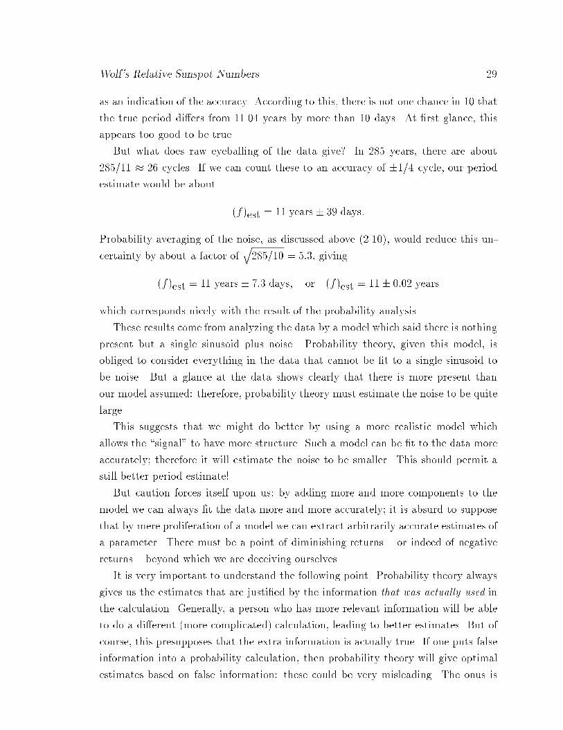
Figure 2.1: Wolf's Relative Sunspot Numbers
SCHUSTER PERIODOGRAM
FAST FOURIER TRANSFORM
STUDENT t-DISTRIBUTION FOR A
SIMPLE HARMONIC FREQUENCY MODEL
Wolf's relative sunspot numbers (A) have been collected on a yearly basis since 1700.The periodogram (B) contains evidence of several complex phenomena. In spite ofthis the single frequency model posterior probability density (C) picks out the 11.04year cycle to an estimated accuracy of �10 days.
Wolf's Relative Sunspot Numbers 29
as an indication of the accuracy. According to this, there is not one chance in 10 that
the true period di�ers from 11.04 years by more than 10 days. At �rst glance, this
appears too good to be true.
But what does raw eyeballing of the data give? In 285 years, there are about
285=11 � 26 cycles. If we can count these to an accuracy of �1=4 cycle, our period
estimate would be about
(f)est = 11 years� 39 days:
Probability averaging of the noise, as discussed above (2.10), would reduce this un-
certainty by about a factor ofq285=10 = 5:3, giving
(f)est = 11 years� 7:3 days; or (f)est = 11� 0:02 years
which corresponds nicely with the result of the probability analysis.
These results come from analyzing the data by a model which said there is nothing
present but a single sinusoid plus noise. Probability theory, given this model, is
obliged to consider everything in the data that cannot be �t to a single sinusoid to
be noise. But a glance at the data shows clearly that there is more present than
our model assumed: therefore, probability theory must estimate the noise to be quite
large.
This suggests that we might do better by using a more realistic model which
allows the \signal" to have more structure. Such a model can be �t to the data more
accurately; therefore it will estimate the noise to be smaller. This should permit a
still better period estimate!
But caution forces itself upon us; by adding more and more components to the
model we can always �t the data more and more accurately; it is absurd to suppose
that by mere proliferation of a model we can extract arbitrarily accurate estimates of
a parameter. There must be a point of diminishing returns { or indeed of negative
returns { beyond which we are deceiving ourselves.
It is very important to understand the following point. Probability theory always
gives us the estimates that are justi�ed by the information that was actually used in
the calculation. Generally, a person who has more relevant information will be able
to do a di�erent (more complicated) calculation, leading to better estimates. But of
course, this presupposes that the extra information is actually true. If one puts false
information into a probability calculation, then probability theory will give optimal
estimates based on false information: these could be very misleading. The onus is

30 CHAPTER 2
always on the user to tell the truth and nothing but the truth; probability theory has
no safety device to detect falsehoods.
The issue just raised takes us into an area that has been heretofore, to the best
of our knowledge, unexplored by any coherent theory. The analysis of this section
has shown how to make the optimum estimates of parameters given a model whose
correctness is not questioned. Deeper probability analysis is needed to indicate how
to make the optimum choice of a model, which neither cheats us by giving poorer
estimates than the data could justify, nor deceives us by seeming to give better es-
timates than the data can justify. But before we can turn to the model selection
problem, the results of this chapter must be generalized to more complex models and
it is to this task that we now turn.
Chapter 3
THE GENERAL MODEL
EQUATION PLUS NOISE
The results of the previous chapter already represent progress on the spectral
analysis problem because we were able to remove consideration of the amplitude,
phase and noise level, and �nd what probability theory has to say about the frequency
alone. In addition, it has given us an indication about how to proceed to more general
problems. If we had used a model where the quadratic term in the likelihood function
did not simplify, we would have a more complicated analytical solution. Although
any multivariate Gaussian integral can be done, the key to being able to remove the
nuisance parameters easily, and above all selectively, was that the likelihood factored
into independent parts. In the full spectrum analysis problem worked on by Jaynes,
[12] the nuisance parameters were not independent, and the explicit solution required
the diagonalization of a matrix that could be quite large.
3.1 The Likelihood Function
To understand an easier approach to complex models, suppose we have a model
of the form
di = f(ti) + ei
f(t) =mXj=1
BjGj(t; f!g): (3:1)
The model functions, Gi(t; f!g), are themselves functions of a set of parameters which
we label collectively f!g (these parameters might be frequencies, chirp rates, decay
31
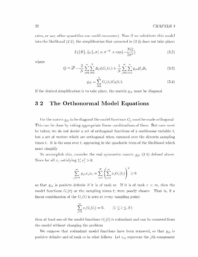
32 CHAPTER 3
rates, or any other quantities one could encounter). Now if we substitute this model
into the likelihood (2.2), the simpli�cation that occurred in (2.3) does not take place:
L(fBg; f!g; �) / ��N � expf�NQ
2�2g (3:2)
where
Q � d2 � 2
N
mXj=1
NXi=1
BjdiGj(ti) +1
N
mXj=1
mXk=1
gjkBjBk (3:3)
gjk =NXi=1
Gj(ti)Gk(ti): (3:4)
If the desired simpli�cation is to take place, the matrix gjk must be diagonal.
3.2 The Orthonormal Model Equations
For the matrix gjk to be diagonal the model functions Gj must be made orthogonal.
This can be done by taking appropriate linear combinations of them. But care must
be taken; we do not desire a set of orthogonal functions of a continuous variable t,
but a set of vectors which are orthogonal when summed over the discrete sampling
times ti. It is the sum over ti appearing in the quadratic term of the likelihood which
must simplify.
To accomplish this, consider the real symmetric matrix gjk (3.4) de�ned above.
Since for all xj satisfyingPx2j > 0,
mXj;k=1
gjkxjxk =NXi=1
0@ mXj=1
xjGj(ti)
1A2
� 0
so that gjk is positive de�nite if it is of rank m. If it is of rank r < m, then the
model functions Gj(t) or the sampling times ti were poorly chosen. That is, if a
linear combination of the Gj(t) is zero at every sampling point:
mXj=1
xjGj(ti) = 0; (1 � i � N)
then at least one of the model functions Gj(t) is redundant and can be removed from
the model without changing the problem.
We suppose that redundant model functions have been removed, so that gjk is
positive de�nite and of rank m in what follows. Let ekj represent the jth component
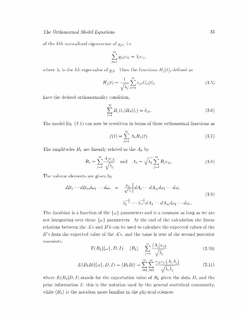
The Orthonormal Model Equations 33
of the kth normalized eigenvector of gjk; i.e.
mXk=1
gjkelk = �lelj;
where �l is the lth eigenvalue of gjk. Then the functions Hj(t), de�ned as
Hj(t) =1q�j
mXk=1
ejkGk(t); (3:5)
have the desired orthonormality condition,
NXi=1
Hj(ti)Hk(ti) = �jk: (3:6)
The model Eq. (3.1) can now be rewritten in terms of these orthonormal functions as
f(t) =mXk=1
AkHk(t): (3:7)
The amplitudes Bk are linearly related to the Ak by
Bk =mXj=1
Ajejkq�j
and Ak =q�k
mXj=1
Bjekj : (3:8)
The volume elements are given by
dB1 � � � dBmd!1 � � � d!r =
���� eljp�j
���� dA1 � � � dAmd!1 � � � d!r
= �� 1
21 � � � ��
12
m dA1 � � � dAmd!1 � � � d!r:
(3:9)
The Jacobian is a function of the f!g parameters and is a constant as long as we are
not integrating over these f!g parameters. At the end of the calculation the linear
relations between the A's and B's can be used to calculate the expected values of the
B's from the expected value of the A's, and the same is true of the second posterior
moments:
E(Bkjf!g;D; I) = hBki =mXj=1
hAjiejkq�j
(3:10)
E(BkBljf!g;D; I) = hBkBli =mXi=1
mXj=1
eikejlhAiAjiq�i�j
(3:11)
where E(BkjD; I) stands for the expectation value of Bk given the data D, and the
prior information I: this is the notation used by the general statistical community,
while hBki is the notation more familiar in the physical sciences.
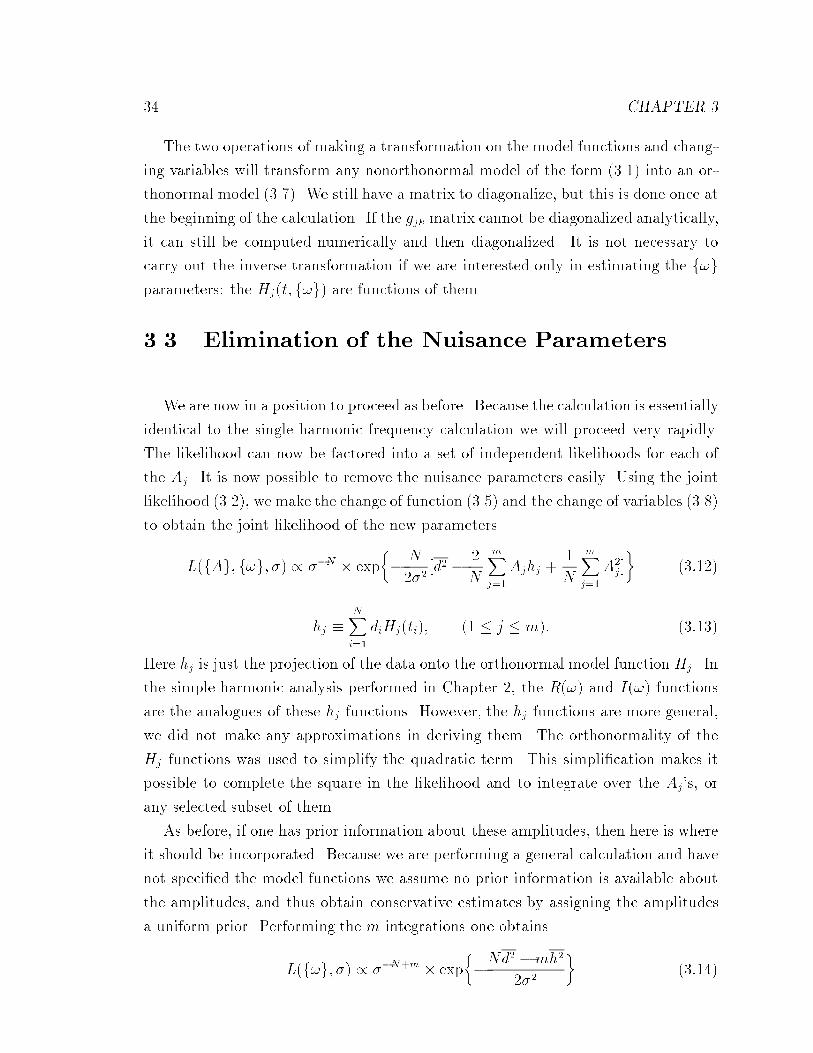
34 CHAPTER 3
The two operations of making a transformation on the model functions and chang-
ing variables will transform any nonorthonormal model of the form (3.1) into an or-
thonormal model (3.7). We still have a matrix to diagonalize, but this is done once at
the beginning of the calculation. If the gjk matrix cannot be diagonalized analytically,
it can still be computed numerically and then diagonalized. It is not necessary to
carry out the inverse transformation if we are interested only in estimating the f!gparameters: the Hj(t; f!g) are functions of them.
3.3 Elimination of the Nuisance Parameters
We are now in a position to proceed as before. Because the calculation is essentially
identical to the single harmonic frequency calculation we will proceed very rapidly.
The likelihood can now be factored into a set of independent likelihoods for each of
the Aj. It is now possible to remove the nuisance parameters easily. Using the joint
likelihood (3.2), we make the change of function (3.5) and the change of variables (3.8)
to obtain the joint likelihood of the new parameters
L(fAg; f!g; �) / ��N � exp�� N
2�2[d2 � 2
N
mXj=1
Ajhj +1
N
mXj=1
A2j ]�
(3:12)
hj �NXi=1
diHj(ti); (1 � j � m): (3:13)
Here hj is just the projection of the data onto the orthonormal model function Hj . In
the simple harmonic analysis performed in Chapter 2, the R(!) and I(!) functions
are the analogues of these hj functions. However, the hj functions are more general,
we did not make any approximations in deriving them. The orthonormality of the
Hj functions was used to simplify the quadratic term. This simpli�cation makes it
possible to complete the square in the likelihood and to integrate over the Aj's, or
any selected subset of them.
As before, if one has prior information about these amplitudes, then here is where
it should be incorporated. Because we are performing a general calculation and have
not speci�ed the model functions we assume no prior information is available about
the amplitudes, and thus obtain conservative estimates by assigning the amplitudes
a uniform prior. Performing the m integrations one obtains
L(f!g; �) / ��N+m � exp��Nd2 �mh2
2�2
�(3:14)
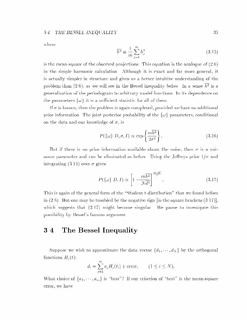
3.4. THE BESSEL INEQUALITY 35
where
h2 � 1
m
mXj=1
h2j (3:15)
is the mean-square of the observed projections. This equation is the analogue of (2.6)
in the simple harmonic calculation. Although it is exact and far more general, it
is actually simpler in structure and gives us a better intuitive understanding of the
problem than (2.6), as we will see in the Bessel inequality below. In a sense h2 is a
generalization of the periodogram to arbitrary model functions. In its dependence on
the parameters f!g it is a su�cient statistic for all of them.
If � is known, then the problem is again completed, provided we have no additional
prior information. The joint posterior probability of the f!g parameters, conditional
on the data and our knowledge of �, is
P (f!gjD;�; I) / exp
(mh2
2�2
): (3:16)
But if there is no prior information available about the noise, then � is a nui-
sance parameter and can be eliminated as before. Using the Je�reys prior 1=� and
integrating (3.14) over � gives
P (f!gjD; I) /"1� mh2
Nd2
#m�N2
: (3:17)
This is again of the general form of the \Student t-distribution" that we found before
in (2.8). But one may be troubled by the negative sign [in the square brackets (3.17)],
which suggests that (3.17) might become singular. We pause to investigate this
possibility by Bessel's famous argument.
3.4 The Bessel Inequality
Suppose we wish to approximate the data vector fd1; � � � ; dNg by the orthogonal
functions Hj(t):
di =mXj=1
ajHj(ti) + error; (1 � i � N):
What choice of fa1; � � � ; amg is \best"? If our criterion of \best" is the mean-square
error, we have
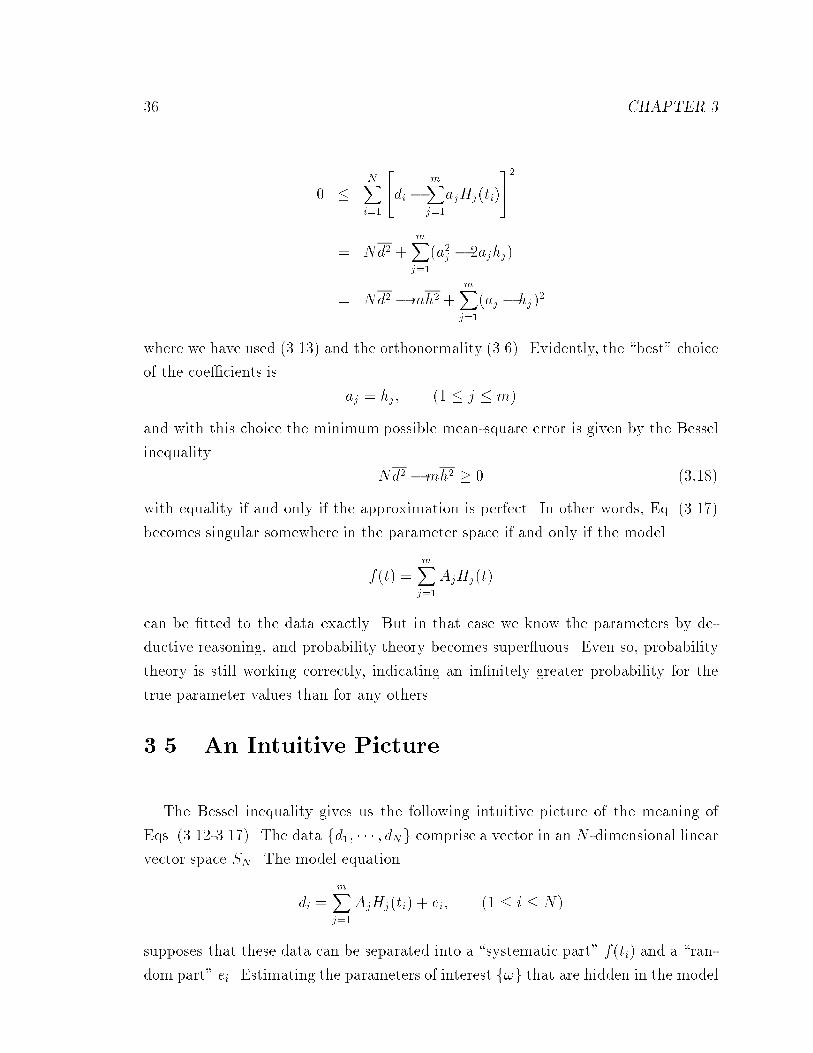
36 CHAPTER 3
0 �NXi=1
24di � mX
j=1
ajHj(ti)
352
= Nd2 +mXj=1
(a2j � 2ajhj)
= Nd2 �mh2 +mXj=1
(aj � hj)2
where we have used (3.13) and the orthonormality (3.6). Evidently, the \best" choice
of the coe�cients is
aj = hj ; (1 � j � m)
and with this choice the minimum possible mean-square error is given by the Bessel
inequality
Nd2 �mh2 � 0 (3:18)
with equality if and only if the approximation is perfect. In other words, Eq. (3.17)
becomes singular somewhere in the parameter space if and only if the model
f(t) =mXj=1
AjHj(t)
can be �tted to the data exactly. But in that case we know the parameters by de-
ductive reasoning, and probability theory becomes super uous. Even so, probability
theory is still working correctly, indicating an in�nitely greater probability for the
true parameter values than for any others.
3.5 An Intuitive Picture
The Bessel inequality gives us the following intuitive picture of the meaning of
Eqs. (3.12-3.17). The data fd1; � � � ; dNg comprise a vector in an N -dimensional linear
vector space SN . The model equation
di =mXj=1
AjHj(ti) + ei; (1 � i � N)
supposes that these data can be separated into a \systematic part" f(ti) and a \ran-
dom part" ei. Estimating the parameters of interest f!g that are hidden in the model

An Intuitive Picture 37
functions Hj(t) amounts essentially to �nding the values of the f!g that permit f(t)
to make the closest possible �t to the data by the mean-square criterion. Put dif-
ferently, probability theory tells us that the most likely values of the f!g are those
that allow a maximum amount of the mean-square data d2 to be accounted for by
the systematic term; from (3.18), those are the values that maximize h2.
However, we have N data points and only m model functions to �t to them.
Therefore, to assign a particular model is equivalent to supposing that the systematic
component of the data lies only in an m-dimensional subspace Sm of SN . What kind
of data should we then expect?
Let us look at the problem backwards for a moment. Suppose someone knows
(never mind how he could know this) that the model is correct, and he also knows
the true values of all the model parameters (fAg; f!g; �) { call this the Utopian state
of knowledge U { but he does not know what data will be found. Then the probability
density that he would assign to any particular data set D = fd1; � � � ; dNg is just ouroriginal sampling distribution (3.2):
P (DjU) = (2��2)�N2 exp
�� 1
2�2
NXi=1
[di � f(ti)]2
�:
From this he would �nd the expectations and covariances of the data:
E(dijU) = hdii = f(ti) (1 � i � N)
hdidji � hdiihdji = (2��2)�N2
ZdNx xixj exp
(� 1
2�2
NXi=1
x2i
)
= �2�ij
therefore he would \expect" to see a value of d2 of about
E(d2jU) = hd2i =1
N
NXi=1
hd2i i
=1
N
NXi=1
(hdii2 + �2)
=1
N
NXi=1
f2(ti) + �2:
(3:19)
But from the orthonormality (3.6) of the Hj(ti), we have
NXi=1
f2(ti) =NXl=1
mXj;k=1
AjAkHj(ti)Hk(ti)
=mXj=1
A2j :

38 CHAPTER 3
So that (3.19) becomes
hd2i = m
NA2 + �2:
Now, what value of h2 would he expect the data to generate? This is
E(h2jU) = hh2i =1
m
mXj=1
hh2j i
=1
m
mXj=1
NXi;k=1
hdidkiHj(ti)Hj(tk)
=1
m
mXj=1
NXi;k=1
(hdiihdki+ �2�ik)Hj(ti)Hj(tk):
(3:20)
ButNXi=1
hdiiHj(ti) =NXi=1
mXl=1
AlHl(ti)Hj(ti)
=mXl=1
Al�lj
= Aj
and (3.20) reduces to
hh2i = A2 + �2:
So he expects the left-hand side of the Bessel inequality (3.18) to be approximately
Nhd2i �mh2 � (N �m)�2: (3:21)
This agrees very nicely with our intuitive judgment that as the number of model
functions increases, we should be able to �t the data better and better. Indeed, when
m = N , the Hj(ti) become a complete orthonormal set on SN , and the data can
always be �t exactly, as (3.21) suggests.
3.6 A Simple Diagnostic Test
If � is known, these results give a simple diagnostic test for judging the adequacy of
our model. Having taken the data, calculate (Nd2�mh2). If the result is reasonably
close to (N �m)�2, then the validity of the model is \con�rmed" (in the sense that
the data give no evidence against the model). On the other hand, if (Nd2 � mh2)

A Simple Diagnostic Test 39
turns out to be much larger than (N �m)�2, the model is not �tting the data as well
as it should: it is \under�tting" the data. That is evidence either that the model is
inadequate to represent the data; we could need more model functions, or di�erent
model functions, or our supposed value of �2 is too low. The next order of business
would be to investigate these possibilities.
It is also possible, although unusual, that (Nd2�mh2) is far less than (N �m)�2;
the model is \over�tting" the data. That is evidence either that our supposed value
of � is too large (the data are actually better than we expected), or that the model
is more complex than it needs to be. By adding more model functions we can always
improve the apparent �t, but if our model functions represent more detail than is
really in the systematic e�ects at work, part of this �t is misleading: we are �tting
the noise.
A test to con�rm this would be to repeat the whole experiment under conditions
where we know the parameters should have the same values as before, and compare the
parameter estimates from the two experiments. Those parameters that are estimated
to be about the same in the two experiments are probably real systematic e�ects. If
some parameters are estimated to be quite di�erent in the two experiments, they are
almost surely spurious: i.e. these are not real e�ects but only artifacts of �tting the
noise. The model should then be simpli�ed, by removing the spurious parameters.
Unfortunately, a repetition is seldom possible with geophysical or economic time
series, although one may split the data into two parts and see if they make about the
same estimates. But repetition is usually easy and standard practice in the controlled
environment of a physics experiment. Indeed, the physicist's common-sense criterion
of a real e�ect is its reproducibility. Probability theory does not con ict with good
common-sense judgment; it only sharpens it and makes it quantitative. A striking
example of this is given in the scenario below.
Consider now the case that � is completely unknown, where probability theory led
us to (3.17). As we show in Appendix C, integrating over a nuisance parameter is
very much like estimating the parameter from the data, and then using that estimate
in our equations. If the parameter is actually well determined by the data, the two
procedures are essentially equivalent. In Chapter 4 we derive an exact expression for
40 CHAPTER 3
the expectation value of the variance h�2i:
h�2i = NN�m�2
"d2 � mh2
N
#
=1
N �m� 2
24 NXi=1
d2i �mXj=1
h2j
35 :
(3:22)
Constraining � to this value, we obtain for the posterior probability of the f!g pa-
rameters approximately
P (f!gjD; h�2i; I) � exp
(mh2
h�2i
):
In e�ect, probability theory tells us that we should apportion the �rst m degrees of
freedom to the signal, the next two to the variance, and the remaining (N �m � 2)
should be noise degrees of freedom. Thus everything probability theory cannot �t to
the signal will be placed in the noise.
More interesting is the opposite extreme when (3.17) approaches a singular value.
Consider the following scenario. You have obtained some data which are recorded
automatically to six �gures and look like this: D = fd1 = 1423:16; d2 = 1509:77; d3 =
1596:38; � � �g. But you have no prior knowledge of the accuracy of those data; for all
you know, � may be as large as 100 or even larger, making the last four digits garbage.
But you plot the data, to determine a model function that best �ts them. Suppose,
for simplicity, that the model function is linear: di = a+si+ei. On plotting di against
i, you are astonished and delighted to see the data falling exactly on a straight line
(i.e. to within the six �gures given). What conclusions do you draw from this?
Intuitively, one would think that the data must be far \better" than had been
thought; you feel sure that � < 10�2, and that you are therefore able to estimate the
slope s to an accuracy considerably better than �10�2, if the number of data values
N is large. It may, however, be hard to see at �rst glance how probability theory can
justify this intuitive conclusion that we draw so easily.
But that is just what (3.17) and (3.22) tell us; Bayesian analysis leads us to it
automatically and for any model functions. Even though you had no reason to expect
it, if it turns out that the data can be �t almost exactly to a model function, then
from the Bessel inequality (3.18) it follows that �2 must be extremely small and, if
the other parameters are independent, they can all be estimated almost exactly.
By \independent" in the last paragraph we mean that a given model function
f(t) =PAjHj(t) can be achieved with only one unique set of values for the pa-

A Simple Diagnostic Test 41
rameters. If several di�erent choices of the parameters all lead to the same model
function, of course the data cannot distinguish between them; only certain functions
of the parameters can be estimated accurately, however many data we have. In this
case the parameters are said to be \confounded" or \unidenti�ed". Generally, this
would be a sign that the model was poorly chosen. However, it may be that the
parameters are known to be real, and the experiment, whether by poor design or the
perversity of nature, is just not capable of distinguishing them.
As an example of confounded parameters, suppose that two di�erent sinusoidal
signals are known to be present, but they have identical frequencies. Then their
separate amplitudes are confounded: the data can give evidence only about their
sum. The di�erence in amplitudes can be known only from prior information.

42 CHAPTER 3
Chapter 4
ESTIMATING THE
PARAMETERS
Once the models had been rewritten in terms of the orthonormal model functions,
we were able to remove the nuisance parameters fAg and �. The integrals performed
in removing the nuisance parameters were all Gaussian or gamma integrals; therefore,
one can always compute the posterior moments of these parameters.
There are a number of reasons why these moments are of interest: the �rst moments
of the amplitudes are needed if one intends to reconstruct the model f(t); the second
moments are related to the energy carried by the signal; the estimated noise variance
�2 and the energy carried by the signal can be used to estimate the signal-to-noise ratio
of the data. Thus the parameters fAg and � are not entirely \nuisance" parameters;
it is of some interest to estimate them. Additionally, we cannot in general compute
the expected value of the f!g parameters analytically. We must devise a procedure
for estimating these parameters and their accuracy.
4.1 The Expected Amplitudes hAji
To begin we will compute the expected amplitudes hAji in the case where the
variance is assumed known. Now the likelihood (3.12) is a function of the f!g pa-
rameters and to estimate the hAji independently of the f!g's, we should integrate
over these parameters. Because we have not speci�ed the model functions, we cannot
do this once and for all. But we can obtain the estimate hAji as functions of the f!gparameters. This gives us what would be the \best" estimate of the amplitudes if we
43

44 CHAPTER 4
knew the f!g parameters.
The expected amplitudes are given by
E(Ajjf!g; �;D; I) = hAji =R+1�1 dA1 � � � dAmAjL(fAg; f!g; �)R+1�1 dA1 � � � dAmL(fAgjf!g; �)
:
We will carry out the �rst integration in detail to illustrate the procedure, and later
just give results. Using the likelihood (3.12) and having no prior information about
Aj, we assign a uniform prior, multiply by Aj and integrate over the fAg. Becausethe joint likelihood is a product of their independent likelihoods, all of the integrals
except the one over Aj cancel:
hAji =R+1�1 dAjAj exp
n� 1
2�2[A2
j � 2Ajhj]o
R+1�1 dAj exp
n� 1
2�2[A2
j � 2Ajhj ]o :
A simple change of variables uj = (Aj � hj)=p2�2 reduces the integrals to
hAji =
R+1�1 duj
�p2�2uj + hj
�exp
n�u2j
oR+1�1 duj exp
n�u2j
o :
The �rst integral in the numerator is zero from symmetry and the second gives
hAji = hj: (4:1)
This is the result one would expect. After all, we are expanding the data on an
orthonormal set of vectors. The expansion coe�cients are just the projections of the
data onto the expansion vectors and that is what we �nd.
We can use these expected amplitudes hAji to calculate the expectation values of
the amplitudes hBji in the nonorthogonal model. Using (3.10), these are given by
E(Bj jf!g; �;D; I) = hBki =mXj=1
hjejkq�j
: (4:2)
Care must be taken in using this formula, because the dependence of the hBki on the
f!g parameters is hidden. The functions hj, the eigenvectors ekj and the eigenvalues
�j are all functions of the f!g parameters. To remove the f!g dependence from (4.2)
one must multiply by P (f!gjD; I) and integrate over all the f!g parameters. If the
total number of f!g parameters r is large this will not be possible. Fortunately, if
the total amount of data is large P (f!gjD; I) will be so nearly a delta function that
we can estimate these parameters from the maximum of P (f!gjD; I).
4.2. THE SECOND POSTERIOR MOMENTS hAJAKi 45
Next we compute hAji when the noise variance �2 is unknown to see if obtaining
independent information about � will a�ect these results. To do this we need the
likelihood L(fAg; f!g); this is given by (3.12) after removing the variance �2 using a
Je�reys prior 1=�:
L(f!g; fAg) /�d2 � mh2
N+
1
N
mXi=1
(Aj � hj)2
��N2
: (4:3)
Using (4.3) and repeating the calculation for hAji one obtains the same result (4.1).
Apparently it does not matter if we know the variance or not. We will make the same
estimate of the amplitudes regardless. As with some of the other results discovered
in this calculation, this is what one's intuition might have said; knowing � a�ects the
accuracy of the estimates but not their actual values. Indeed, the �rst moments were
independent of the value of � when the variance was known; it is hard to see how the
�rst moments could suddenly become di�erent when the variance is unknown.
4.2 The Second Posterior Moments hAjAki
The second posterior moments hAjAki cannot be independent of the noise variance�2, for that is what limits the accuracy of our estimates of the Aj. The second
posterior moments, when the variance is assumed known, are given by
E(AjAkjf!g; �;D; I) = hAjAki =R+1�1 dA1 � � � dAmAjAkL(fAg; f!g; �)R+1
�1 dA1 � � � dAmL(fAg; f!g; �):
Using the likelihood (3.12) and again assuming a uniform prior, these expectation
values are given by
hAjAki = hjhk + �2�jk
so that, in view of (4.1), the posterior covariances are
hAjAki � hAjihAki = �2�jk: (4:4)
The Aj parameters are uncorrelated (we de�ned the model functions Hj(t) to ensure
this), and each one is estimated to an accuracy ��. Intuitively, we might anticipate
this but we would not feel very sure of it.
The expectation value hAjAki may be related to the expectation value for the
original model amplitudes by using (3.11):
hBkBli � hBkihBli = �2mXj=1
ejkejl
�j: (4:5)
46 CHAPTER 4
These are the explicit Bayesian estimates for the posterior covariances for the original
model. These are the most conservative estimates (in the sense discussed before) one
can make, but they are still functions of the f!g parameters.
We can repeat these calculations for the second posterior moments in the case
when � is assumed unknown to see if obtaining explicit information about � is of use.
Of course, we expect the results to di�er from the previous result since (4.5) depends
explicitly on �. Performing the required calculation gives
E(AjAkjf!g;D; I) = hAjAki = hjhk
+�
N
N � 2
� �2N � 5
2N � 5 � 2m
� �2N � 7
2N � 7 � 2m
� "d2 � mh2
N
#�jk:
Comparing this with (4.4) shows that obtaining independent information about � will
a�ect the estimates of the second moments. But not by much, as we will see below.
The second term in this equation is essentially an estimate of �2, but for small N it
di�ers appreciably from the direct estimate found next.
4.3 The Estimated Noise Variance h�2i
One of the things that is of interest in an experiment is to estimate the noise power
�2. This indicates how \good" the data appear to be in the light of the model, and
can help one in making many judgments, such as whether to try a new model or build
a new apparatus. We can obtain the expected value of � as a function of the f!gparameters; however, we can just as easily obtain the posterior moments h�si for anypower s. Using (3.14), and the Je�reys prior 1=�, we integrate:
E(�sjf!g;D; I) = h�si =R+10 d��s�1L(�jf!g;D; I)R+10 d���1L(�jf!g;D; I)
to obtain
h�si = ��N �m� s
2
���N �m
2
��1�Nd2 �mh2
2
� s2
: (4:6)
For s = 2 this gives the estimated variance as
h�2i =N
N �m� 2
�d2 � mh2
N
�
=1
N �m� 2
� NXi=1
d2i �mXj=1
h2j
�:
(4:7)
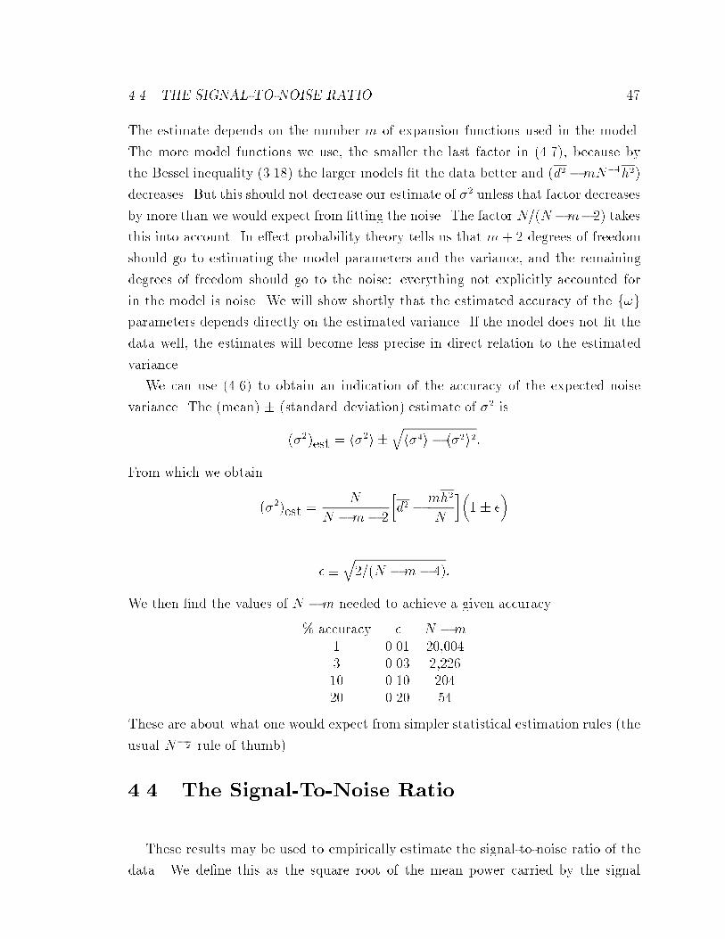
4.4. THE SIGNAL-TO-NOISE RATIO 47
The estimate depends on the number m of expansion functions used in the model.
The more model functions we use, the smaller the last factor in (4.7), because by
the Bessel inequality (3.18) the larger models �t the data better and (d2 �mN�1h2)
decreases. But this should not decrease our estimate of �2 unless that factor decreases
by more than we would expect from �tting the noise. The factor N=(N�m�2) takes
this into account. In e�ect probability theory tells us that m+ 2 degrees of freedom
should go to estimating the model parameters and the variance, and the remaining
degrees of freedom should go to the noise: everything not explicitly accounted for
in the model is noise. We will show shortly that the estimated accuracy of the f!gparameters depends directly on the estimated variance. If the model does not �t the
data well, the estimates will become less precise in direct relation to the estimated
variance.
We can use (4.6) to obtain an indication of the accuracy of the expected noise
variance. The (mean) � (standard deviation) estimate of �2 is
(�2)est = h�2i �qh�4i � h�2i2:
From which we obtain
(�2)est =N
N �m� 2
�d2 � mh2
N
��1 � �
�
� �q2=(N �m� 4):
We then �nd the values of N �m needed to achieve a given accuracy
% accuracy � N �m
1 0.01 20,0043 0.03 2,22610 0.10 20420 0.20 54
These are about what one would expect from simpler statistical estimation rules (the
usual N� 12 rule of thumb).
4.4 The Signal-To-Noise Ratio
These results may be used to empirically estimate the signal-to-noise ratio of the
data. We de�ne this as the square root of the mean power carried by the signal

48 CHAPTER 4
divided by the mean power carried by the noise:
Signal
Noise=�hmXj=1
A2j i=N�2
� 12
:
This may be obtained from (4.2):
Signal
Noise=�m
N
�1 +
h2
�2
�� 12
: (4:8)
A similar empirical signal-to-noise ratio may be obtained when the noise variance �
is unknown by replacing � in (4.8) by the estimated noise variance (4.7). When the
data �t the model so well that h2 � �2, the estimate reduces to
�mh2
N�2
� 12
or�Pm
j=1 h2jPN
k=1 e2i
� 12
We will compute the signal-to-noise ratio for several models in the following sections.
4.5 Estimating the {!} Parameters
Unlike the amplitudes fAg and the variance �2, we cannot calculate the expecta-
tion values of the f!g parameters analytically. In general, the integrals represented
by
h!ji =Zd!1 � � � d!r !j P (f!gjD; I)
cannot be done exactly. Nonetheless we must obtain an estimate of these parameters,
and their probable accuracy.
The exact joint posterior density is (3.16) when � is known, and (3.17) when it is
not. But they are not very di�erent provided we have enough data for good estimates.
For, writing the maximum attainablePh2j as0
@ mXj=1
h2j
1Amax
= x
and writing the di�erence from the maximum as q2 i.e.
mXj=1
h2j = x� q2;
Eq. (3.17) becomes
"NXi=1
d2i � x+ q2#m�N
2
� exp
(� (N �m)q2
2(PN
j=1 d2i � x)
):

Estimating the {!} Parameters 49
But this is nearly the same as
"NXi=1
d2i � x+ q2#m�N
2
� exp
(� q2
2h�2i
)
where we used the estimate (4.7) for �2 evaluated for the values f!g that maximize
the posterior probability as a function of the f!g parameters. So up to an irrelevant
normalization constant the posterior probability of the f!g parameters around the
location of the maximum is given by
P (f!gjD; h�2i; I) � exp�mh2
2h�2i
�(4:9)
where the slightly inconsistent notation P (f!gjh�2i;D; I) has been adopted to remind
us that we have used h�2i, not �2. We have noted before that when we integrate over
a nuisance parameter, the e�ect is for most purposes to estimate the parameter from
the data, and then constrain the parameter to that value.
We expand h2, to obtain q2, in a Taylor series around the maximum f!g to obtain
P (f!gjD; h�2i; I) / exp��
rXjk=1
bjk
2h�2i�j�k
�(4:10)
where bjk is the analogue of (2.9) de�ned in the single harmonic frequency problem
bjk � �m
2
@2h2
@!j@!k(4:11)
�j � !j � !j :
From (4.10) we can make the (mean) � (standard deviation) approximations for
the f!g parameters. We do these Gaussian integrals by �rst changing to orthogonal
variables and then perform the r integrals just as we did with the amplitudes in
Chapter 3. The new variables are obtained from the eigenvalues and eigenvectors of
bjk. Let ujk denote the kth component of the jth eigenvector of bjk and let vj be the
eigenvalue. The orthogonal variables are given by
sj =pvj
rXk=1
�kukj �j =rX
k=1
skujkpvk
:
Making this change of variables, we have
P (fsgjh�2i;D; I) / v� 1
21 � � � v�
12
r exp��
rXj=1
s2j
2h�2i
�: (4:12)

50 CHAPTER 4
From (4.12) we can compute hsji and hs2j i. Of course hsji is zero and the expectation
value hsjski is given by
hsksji =
R1�1 ds1 � � � dsrv
� 12
1 � � � v�12
r sksj exp��
rXl=1
s2l2h�2i
�
R1�1 ds1 � � � dsrv
� 12
1 � � � v�12
r exp��
rXl=1
s2l2h�2i
�
hsksji = h�2i�kj
where �kj is a Kronecker delta function. In the posterior distribution the sj are
uncorrelated, as they should be. From this we may obtain the posterior covariances
of the f!g parameters. These are
h!j!ki � h!jih!ki = h�2irX
l=1
uljulk
vl;
and the variance 2k of the posterior distribution for !k is
2k � h�2irX
j=1
u2jk
vj: (4:13)
Then the estimated !j parameters are
(!j)est = !j � j (4:14)
and; here !j is the location of the maximum of the probability distribution as a
function of the f!g parameter.
For an arbitrary model the matrix bjk cannot be calculated analytically; however,
it can be evaluated numerically using the computer code given in Appendix E. We
use a general searching routine to �nd the maximum of the probability distribution
and then calculate this matrix numerically. The log of the \Student t-distribution"
is so sharply peaked that gradient searching routines do not work well. We use a
\pattern" search routine described by Hooke and Jeeves [21] [22].
The accuracy estimates of both the f!g parameters and the amplitudes fAg in
Eq. (4.5) depend explicitly on the estimated noise variance. But the estimated vari-
ance is the mean square di�erence between the model and the data. If the mis�t is
large the variance is estimated to be large and the accuracy is estimated to be poor.
Thus when we say that the parameter estimates are conservative we mean that, be-
cause everything probability theory cannot �t to the model is assigned to the noise,
all of our parameter estimates are as wide as is consistent with the model and the

4.6. THE POWER SPECTRAL DENSITY 51
data. For example, when we estimate a frequency from a discrete Fourier transform
we are in e�ect using a single harmonic frequency model for an estimate (position of
a peak). But the width of the peak has nothing to do with the noise level, and if
we supposed it, erroneously, to be an indication of the accuracy of our estimate, we
could make very large errors.
This is perhaps one of the most subtle and important points about the use of
uninformative priors that comes out in this work, and we will try to state it more
clearly. When we did this calculation, at every point where we had to supply a prior
probability we chose a prior that was as uninformative as possible (by uninformative
we mean that the prior is as smooth as it can be and still be consistent with the
known information). Speci�cally we mean a prior that has no sharp maximum: one
that does not determine any value of the parameter strongly. We derived the Gaussian
for the noise prior as the smoothest, least informative, prior that was consistent with
the given second moment of the noise. We speci�cally did not assume the noise was
nonwhite or correlated because we do not have prior information to that e�ect. So if
the noise turns out to be colored we have in e�ect already allowed for that possibility
because we used a less informative prior for the noise, which automatically considers
every possible way of being colored, in the sense that the white noise basic support
set includes all those of colored noise. On the other hand, if we knew a speci�c way in
which the noise departs from whiteness, we could exploit that information to obtain
a more concentrated noise probability distribution, leading to still better estimates of
the f!g parameters. We will demonstrate this point several times in Chapter 6.
4.6 The Power Spectral Density
Although not explicitly stated, we have calculated above an estimate of the total
energy of the signal. The total energy E carried by the signal in our orthogonal model
is
E �Z tN
t1
f(t)2dt �mXj=1
A2j
and its spectral density is given by
p(f!g) = m
��2 + h2
�P (f!gjD; I; �): (4:15)
This function is the energy per unit f!g carried by the signal (not the noise). This
power spectral estimate is essentially a power normalized probability distribution,
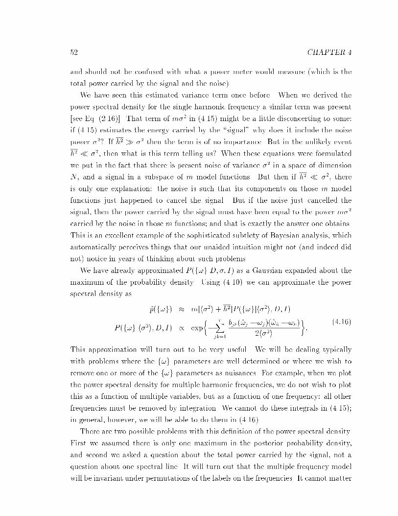
52 CHAPTER 4
and should not be confused with what a power meter would measure (which is the
total power carried by the signal and the noise).
We have seen this estimated variance term once before. When we derived the
power spectral density for the single harmonic frequency a similar term was present
[see Eq. (2.16)]. That term of m�2 in (4.15) might be a little disconcerting to some;
if (4.15) estimates the energy carried by the \signal" why does it include the noise
power �2? If h2 � �2 then the term is of no importance. But in the unlikely event
h2 � �2, then what is this term telling us? When these equations were formulated
we put in the fact that there is present noise of variance �2 in a space of dimension
N , and a signal in a subspace of m model functions. But then if h2 � �2, there
is only one explanation: the noise is such that its components on those m model
functions just happened to cancel the signal. But if the noise just cancelled the
signal, then the power carried by the signal must have been equal to the power m�2
carried by the noise in those m functions; and that is exactly the answer one obtains.
This is an excellent example of the sophisticated subtlety of Bayesian analysis, which
automatically perceives things that our unaided intuition might not (and indeed did
not) notice in years of thinking about such problems.
We have already approximated P (f!gjD;�; I) as a Gaussian expanded about the
maximum of the probability density. Using (4.10) we can approximate the power
spectral density as
p(f!g) � m[h�2i+ h2]P (f!gjh�2i;D; I)
P (f!gjh�2i;D; I) / exp��
rXjk=1
bjk(!j � !j)(!k � !k)
2h�2i
�:
(4:16)
This approximation will turn out to be very useful. We will be dealing typically
with problems where the f!g parameters are well determined or where we wish to
remove one or more of the f!g parameters as nuisances. For example, when we plot
the power spectral density for multiple harmonic frequencies, we do not wish to plot
this as a function of multiple variables, but as a function of one frequency: all other
frequencies must be removed by integration. We cannot do these integrals in (4.15);
in general, however, we will be able to do them in (4.16).
There are two possible problems with this de�nition of the power spectral density.
First we assumed there is only one maximum in the posterior probability density,
and second we asked a question about the total power carried by the signal, not a
question about one spectral line. It will turn out that the multiple frequency model
will be invariant under permutations of the labels on the frequencies. It cannot matter
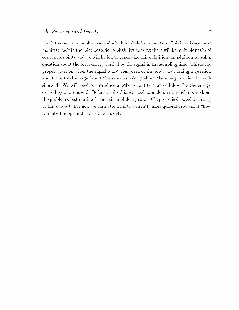
The Power Spectral Density 53
which frequency is number one and which is labeled number two. This invariance must
manifest itself in the joint posterior probability density; there will be multiple peaks of
equal probability and we will be led to generalize this de�nition. In addition we ask a
question about the total energy carried by the signal in the sampling time. This is the
proper question when the signal is not composed of sinusoids. But asking a question
about the total energy is not the same as asking about the energy carried by each
sinusoid. We will need to introduce another quantity that will describe the energy
carried by one sinusoid. Before we do this we need to understand much more about
the problem of estimating frequencies and decay rates. Chapter 6 is devoted primarily
to this subject. For now we turn attention to a slightly more general problem of \how
to make the optimal choice of a model?"

54 CHAPTER 4

Chapter 5
MODEL SELECTION
When analyzing the results of an experiment it is not always known which model
function (3.1) applies. We need a way to choose between several possible models.
This is easily done using Bayes' theorem (1.3) and repeated applications of the proce-
dure (1.4) which led to the \Student t-distribution." The �rst step in answering this
question is to enumerate the possible models. Suppose we have a set of s possible
models fH1; � � � ;Hsg with model functions ff1; � � � ; fsg. We are hardly ever sure that
the \true" model is actually contained in this set. Indeed, the \set of all possible
models" is not only in�nite, but it is also quite unde�ned. It is not even clear what
one could mean by a \true" model; both questions may take us into an area more
like theology than science.
The only questions we seek to examine here are the ones that are answerable
because they are mathematically well-posed. Such questions are of the form: \Given
a speci�ed set Ss of possible models fH1; � � � ;Hsg and looking only within that set,
which model is most probable in view of all the data and prior information, and how
strongly is it supported relative to the alternatives in that set?" Bayesian analysis
can give a de�nite answer to such a question { see [15], [23].
5.1 What About \Something Else?"
To say that we con�ne ourselves to the set Ss is not to assert dogmatically that
there are no other possibilities; we may assign prior probabilities P (Hj jI); (1 � j � s)
55
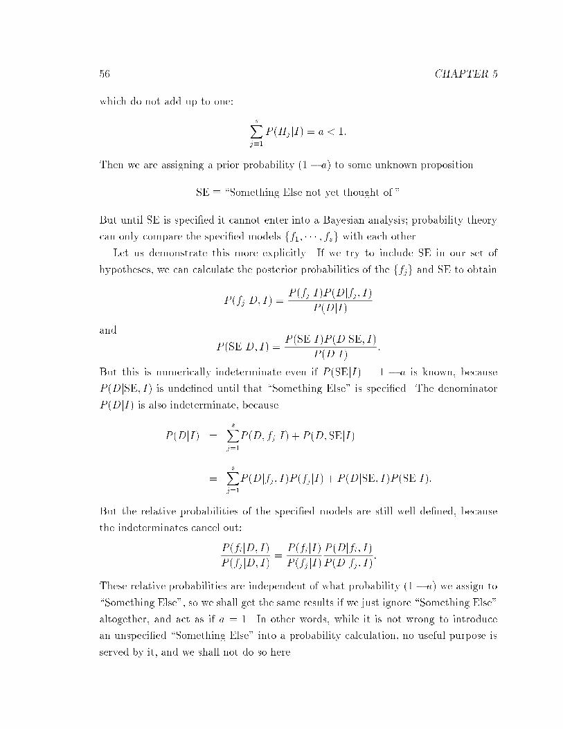
56 CHAPTER 5
which do not add up to one:
sXj=1
P (Hj jI) = a < 1:
Then we are assigning a prior probability (1� a) to some unknown proposition
SE � \Something Else not yet thought of."
But until SE is speci�ed it cannot enter into a Bayesian analysis; probability theory
can only compare the speci�ed models ff1; � � � ; fsg with each other.
Let us demonstrate this more explicitly. If we try to include SE in our set of
hypotheses, we can calculate the posterior probabilities of the ffjg and SE to obtain
P (fjjD; I) =P (fjjI)P (Djfj ; I)
P (DjI)
and
P (SEjD; I) = P (SEjI)P (DjSE; I)P (DjI) :
But this is numerically indeterminate even if P (SEjI) = 1 � a is known, because
P (DjSE; I) is unde�ned until that \Something Else" is speci�ed. The denominator
P (DjI) is also indeterminate, because
P (DjI) =sX
j=1
P (D; fj jI) + P (D;SEjI)
=sX
j=1
P (Djfj ; I)P (fjjI) + P (DjSE; I)P (SEjI):
But the relative probabilities of the speci�ed models are still well de�ned, because
the indeterminates cancel out:
P (fijD; I)P (fj jD; I)
=P (fijI)P (fj jI)
P (Djfi; I)P (Djfj ; I)
:
These relative probabilities are independent of what probability (1� a) we assign to
\Something Else", so we shall get the same results if we just ignore \Something Else"
altogether, and act as if a = 1. In other words, while it is not wrong to introduce
an unspeci�ed \Something Else" into a probability calculation, no useful purpose is
served by it, and we shall not do so here.

5.2. THE RELATIVE PROBABILITY OF MODEL FJ 57
5.2 The Relative Probability of Model fj
We wish to con�ne our attention to a selected set of models ff1; � � � ; fsg. Becauseof the arguments just given we may write
sXj=1
P (fj jD; I) = 1
where P (fjjD; I) is the posterior probability of model fj. From Bayes' theorem (1.3)
we may write
P (fjjD; I) =P (fjjI)P (Djfj ; I)
P (DjI)(5:1)
and
P (DjI) =sX
j=1
P (fjjI)P (Djfj ; I):
The way to proceed on this problem is to apply the general procedure for removing
nuisance parameters given in Chapter 1. We will assume for now that the variance
of the noise �2 is known and derive P (fjj�;D; I), then at the end of the calculation
if � is not known we will remove it. Thus symbolically, we have
P (Dj�; fj ; I) =ZdfAgdf!gP (fAg; f!gjI)P (DjfAg; f!g; �; fj; I): (5:2)
But this is essentially just the problem we solved in Chapter 3 [Eqs. (3.12-3.17)]
with three additions: when there can be di�ering numbers of parameters we must
use normalized priors, we must do the integrals over the f!g parameters, and the
direct probability Eq. (5.2) of the data for the jth model must include all numerical
factors in P (DjfAg; f!g; �; fj; I). We will need to keep track of the normalization
constants explicitly because the results we obtain will depend on them. We will do
this calculation in four steps; �rst perform the integrals over the amplitudes fAgusing an appropriately normalized prior. Second we approximate the quasi-likelihood
of the f!g parameters about the maximum likelihood point; third remove the f!gparameters by integration; and fourth remove the variances (plural because two more
variances appear before we �nish the calculation). Because the calculation is lengthy,
we make many approximations of the kind that experienced users of applied math-
ematics learn to make. They could be avoided { but the calculation would then be
much longer, with the same �nal conclusions.
We begin by the calculation in a manner similar to that done in Chapter 3. The
question we would like to ask is \Given a set of model equations ff1; � � � ; fsg and

58 CHAPTER 5
looking only within that set, which model best accounts for the data?" We will take
fj(t) =mXk=1
AkHk(t; f!g)
as our model, where Hk are the orthonormal model functions de�ned earlier, Eq. (3.5).
The subscripts \j" refers to the jth member of the set of models ff1; � � � ; fsg, withthe understanding that the amplitudes fAg, the nonlinear f!g, the total number of
model functions m, and the model functions Hk(t; f!g) are di�erent for every fj.
We could label each of these with an additional subscript, for example Hjk to stand
for model function k of model fj ; however, we will not do this simply because the
proliferation of subscripts would render the mathematics unreadable.
To calculate the direct probability of the data given model fj we take the di�erence
between the data and the model. This di�erence is the noise, if the model is true,
and making the most conservative assumptions possible about the noise we assign a
Gaussian prior for the noise. This gives the
P (DjfAg; f!g; �; fj; I) = (2��2)�N2 exp
(� 1
2�2
NXi=1
[di � fj(ti)]2
)
as the direct probability of the data given model fj and the parameters. Now ex-
panding the square we obtain
P (DjfAg; f!g; �; fj; I) = (2��2)�N2 exp
��NQ
2�2
�
where
Q � d2 � 2
N
mXl=1
Alhl +1
N
mXl=1
A2l
andNXi=1
Hl(ti)Hk(ti) = �lk
and
hl =NXi=1
diHl(ti)
was used to simplify the expression. This is now substituted back into Eq. (5.2) to
obtain
P (Dj�; fj ; I) =ZdfAgdf!gP (fAg; f!gjI)(2��2)�
N2 exp
��NQ
2�2
�: (5:3)
At this point in the calculation we have simply repeated the steps done in Chap-
ter 3 with one exception: we have retained the normalization constants in the direct
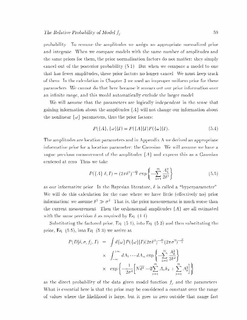
The Relative Probability of Model fj 59
probability. To remove the amplitudes we assign an appropriate normalized prior
and integrate. When we compare models with the same number of amplitudes and
the same priors for them, the prior normalization factors do not matter: they simply
cancel out of the posterior probability (5.1). But when we compare a model to one
that has fewer amplitudes, these prior factors no longer cancel. We must keep track
of them. In the calculation in Chapter 3 we used an improper uniform prior for these
parameters. We cannot do that here because it smears out our prior information over
an in�nite range, and this would automatically exclude the larger model.
We will assume that the parameters are logically independent in the sense that
gaining information about the amplitudes fAg will not change our information about
the nonlinear f!g parameters, thus the prior factors:
P (fAg; f!gjI) = P (fAgjI)P (f!gjI): (5:4)
The amplitudes are location parameters and in Appendix A we derived an appropriate
informative prior for a location parameter: the Gaussian. We will assume we have a
vague previous measurement of the amplitudes fAg and express this as a Gaussian
centered at zero. Thus we take
P (fAgj�; I) = (2��2)�m2 exp
(�
mXk=1
A2k
2�2
)(5:5)
as our informative prior. In the Bayesian literature, � is called a \hyperparameter".
We will do this calculation for the case where we have little (e�ectively no) prior
information: we assume �2 � �2. That is, the prior measurement is much worse than
the current measurement. Then the orthonormal amplitudes fAg are all estimated
with the same precision � as required by Eq. (4.4).
Substituting the factored prior, Eq. (5.4), into Eq. (5.3) and then substituting the
prior, Eq. (5.5), into Eq. (5.3) we arrive at
P (Dj�; �; fj ; I) =Zdf!gP (f!gjI)(2��2)�m
2 (2��2)�N2
�Z +1
�1dA1 � � � dAm exp
(�
mXk=1
A2k
2�2
)
� exp
(� 1
2�2
�Nd2 � 2
mXk=1
Akhk +mXk=1
A2k
�)
as the direct probability of the data given model function fj and the parameters.
What is essential here is that the prior may be considered a constant over the range
of values where the likelihood is large, but it goes to zero outside that range fast
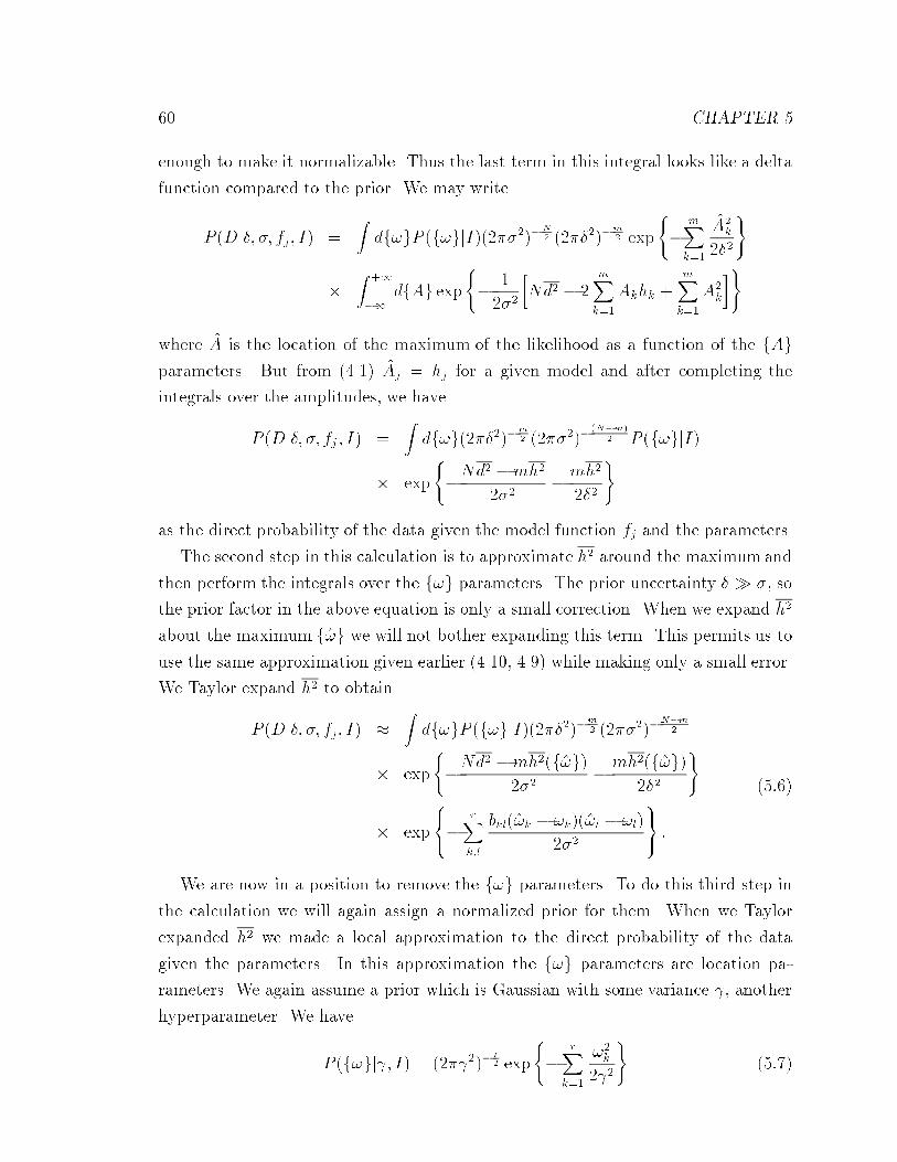
60 CHAPTER 5
enough to make it normalizable. Thus the last term in this integral looks like a delta
function compared to the prior. We may write
P (Dj�; �; fj; I) =Zdf!gP (f!gjI)(2��2)�
N2 (2��2)�
m2 exp
(�
mXk=1
A2k
2�2
)
�Z +1
�1dfAg exp
(� 1
2�2
�Nd2 � 2
mXk=1
Akhk +mXk=1
A2k
�)
where A is the location of the maximum of the likelihood as a function of the fAgparameters. But from (4.1) Aj = hj for a given model and after completing the
integrals over the amplitudes, we have
P (Dj�; �; fj ; I) =Zdf!g(2��2)�m
2 (2��2)�(N�m)
2 P (f!gjI)
� exp
(�Nd2 �mh2
2�2� mh2
2�2
)
as the direct probability of the data given the model function fj and the parameters.
The second step in this calculation is to approximate h2 around the maximum and
then perform the integrals over the f!g parameters. The prior uncertainty � � �, so
the prior factor in the above equation is only a small correction. When we expand h2
about the maximum f!g we will not bother expanding this term. This permits us to
use the same approximation given earlier (4.10, 4.9) while making only a small error.
We Taylor expand h2 to obtain
P (Dj�; �; fj; I) �Zdf!gP (f!gjI)(2��2)�m
2 (2��2)�N�m
2
� exp
(�Nd2 �mh2(f!g)
2�2� mh2(f!g)
2�2
)
� exp
8<:�
rXk;l
bkl(!k � !k)(!l � !l)
2�2
9=; :
(5:6)
We are now in a position to remove the f!g parameters. To do this third step in
the calculation we will again assign a normalized prior for them. When we Taylor
expanded h2 we made a local approximation to the direct probability of the data
given the parameters. In this approximation the f!g parameters are location pa-
rameters. We again assume a prior which is Gaussian with some variance , another
hyperparameter. We have
P (f!gj ; I) = (2� 2)�r2 exp
(�
rXk=1
!2k
2 2
)(5:7)
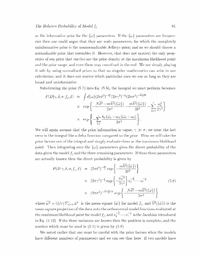
The Relative Probability of Model fj 61
as the informative prior for the f!g parameters. If the f!g parameters are frequen-
cies then one could argue that they are scale parameters, for which the completely
uninformative prior is the nonnormalizable Je�reys prior; and so we should choose a
normalizable prior that resembles it. However, that does not matter; the only prop-
erties of our prior that survive are the prior density at the maximum likelihood point
and the prior range, and even these may cancel out in the end. We are simply playing
it safe by using normalized priors so that no singular mathematics can arise in our
calculation; and it does not matter which particular ones we use as long as they are
broad and uninformative.
Substituting the prior (5.7) into Eq. (5.6), the integral we must perform becomes
P (Dj ; �; �; fj; I) �Zdf!g(2��2)�m
2 (2� 2)�r2 (2��2)�
N�m2
� exp
(�Nd2 �mh2(f!g)
2�2� mh2(f!g)
2�2�
rXk=1
!2k
2 2
)
� exp
8<:�
rXk;l
bkl(!k � !k)(!l � !l)
2�2
9=; :
We will again assume that the prior information is vague, � �, we treat the last
term in the integral like a delta function compared to the prior. Thus we will take the
prior factors out of the integral and simply evaluate them at the maximum likelihood
point. Then integrating over the f!g parameters gives the direct probability of the
data given the model fj and the three remaining parameters. If these three parameters
are actually known then the direct probability is given by
P (Dj ; �; �; fj ; I) = (2��2)�m2 exp
(�mh2(f!g)
2�2
)
� (2� 2)�r2 exp
(�r!
2
2 2
)v� 1
21 � � � v�
12
r
� (2��2)�N�m�r
2 exp
(�Nd2 �mh2(f!g)
2�2
)(5:8)
where !2 = (1=r)Pr
k=1 !2 is the mean-square f!g for model fj, and h2(f!g) is the
mean-square projection of the data onto the orthonormal model functions evaluated at
the maximumlikelihood point for model fj , and v� 1
21 � � � v�
12
r is the Jacobian introduced
in Eq. (4.12). If the three variances are known then the problem is complete, and the
number which must be used in (5.1) is given by (5.8).
We noted earlier that one must be careful with the prior factors when the models
have di�erent numbers of parameters and we can see that here. If two models have
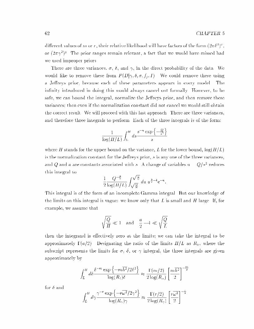
62 CHAPTER 5
di�erent values ofm or r, their relative likelihood will have factors of the form (2��2)x,
or (2� 2)y. The prior ranges remain relevant, a fact that we would have missed had
we used improper priors.
There are three variances, �, �, and , in the direct probability of the data. We
would like to remove these from P (Dj ; �; �; fj ; I). We could remove these using
a Je�reys prior, because each of these parameters appears in every model. The
in�nity introduced in doing this would always cancel out formally. However, to be
safe, we can bound the integral, normalize the Je�reys prior, and then remove these
variances; then even if the normalization constant did not cancel we would still obtain
the correct result. We will proceed with this last approach. There are three variances,
and therefore three integrals to perform. Each of the three integrals is of the form:
1
log(H=L)
Z H
Ldss�a exp
n�Q
s2
os
whereH stands for the upper bound on the variance, L for the lower bound, log(H=L)
is the normalization constant for the Je�reys prior, s is any one of the three variances,
and Q and a are constants associated with s. A change of variables u = Q=s2 reduces
this integral to
1
2
Q�a2
log(H=L)
Z pQ
LpQ
H
du ua2�1e�u:
This integral is of the form of an incomplete Gamma integral. But our knowledge of
the limits on this integral is vague: we know only that L is small and H large. If, for
example, we assume that
sQ
H� 1 and
a
2� 1�
sQ
L
then the integrand is e�ectively zero at the limits; we can take the integral to be
approximately �(a=2). Designating the ratio of the limits H=L as R�, where the
subscript represents the limits for �, �, or integral, the three integrals are given
approximately by
Z H
Ld���m exp
n�mh2=2�2
olog(R�)�
� �(m=2)
2 log(R�)
"mh2
2
#�m2
for � and Z H
Ld
�r expn�r!2=2 2
olog(R )
� �(r=2)
2 log(R )
"r!2
2
#� r2
5.3. ONE MORE PARAMETER 63
for and
Z H
Ld�
�m+r�N expn�[Nd2 �mh2]=2�2
olog(R�)�
��(N�m�r
2)
2 log(R�)
"Nd2 �mh2(f!g)
2
#m+r�N2
for �.
Using these three integrals the global likelihood of the data given the model fj is
given by
P (Djfj ; I) =�(m=2)2 log(R�)
"mh2(f!g)
2
#�m2 �(r=2)2 log(R )
"r!2
2
#� r2
v� 1
21 � � � v�
12
r
� �([N �m� r]=2)2 log(R�)
"Nd2 �mh2(f!g)
2
#m+r�N2
:
(5:9)
The three factors involved in normalizing the Je�reys priors appear in every model:
they always cancel as long as we deal with models having all three types of parameters.
However, as soon as we try to compare a model involving two types of parameters to
a model involving all three types of parameters (e.g. a regression model to a nonlinear
model) they no longer cancel: the prior ranges become important. One must think
carefully about just what prior information one actually has about , and �, and use
that information to set their prior ranges. As we shall see in what follows, if the
data actually determine the model parameters well (so that these equations apply)
the actual values one assigns to � and are relatively unimportant.
5.3 One More Parameter
We would like to understand (5.1), (5.8), and (5.9) better, and we present here a
simple example of their use. Suppose we are dealing with the simplest model selection
possible: expanding the data on a set of model functions. A typical set of model
functions might be polynomials. This is the simplest model possible because there
are no f!g parameters; only amplitudes. But suppose further that we choose our
model functions so that they are already orthogonal in the sense de�ned earlier. All
that is left for us to decide is \When have we incorporated enough expansion vectors
to adequately represent the signal?" We will assume in this demonstration that both
the variance � and the prior variance � are known and apply (5.8). Further, we will
be comparing only two models at a time, and will compute the ratio of Eq. (5.8) for
a model containing m expansion functions (or vectors on the discrete sample points)
64 CHAPTER 5
to a model containing m + 1 expansion functions. This ratio is called the posterior
\odds" in favor of the smaller model.
When we have m expansion vectors and no f!g, Eq. (5.8) reduces to
P (Djfm; �; �; I) = (2��2)�m2 exp
(�
mXk=1
h2k2�2
)
� (2��2)�N�m
2 exp
(� 1
2�2
"Nd2 �
mXk=1
h2k
#)
for the �rst model and to
P (Djfm+1; I) = (2��2)�m+12 exp
(�
m+1Xk=1
h2k2�2
)
� (2��2)�N�m�1
2 exp
(� 1
2�2
"Nd2 �
m+1Xk=1
h2k
#)
for a model with m+ 1 parameters. Because these models are already orthonormal,
hk is the same in both equations: when we compute the odds ratio all but the last will
cancel. Thus the posterior odds ratio simpli�es considerably. We have the likelihood
ratio
L =P (Djfm; �; �; I)P (Djfm+1; �; �; I)
=�
�exp
(�1
�2� 1
�2
�h2m+1
2
):
The posterior odds ratio then involves the posterior probabilities:
P (fmj�; �;D; I)P (fm+1j�; �;D; I)
=P (fmjI)P (fm+1jI)
L:
We derived this approximation assuming �� �, so we have
L =�
�exp
(�h
2m+1
2�2
):
In other words, the smaller model is helped by uncertainty in the prior knowledge
of Am+1, while the larger model is helped by the relative size of the estimated next
amplitude compared to the noise. This is the Bayesian quantitative version of Occam's
razor: prefer the simpler model unless the bigger one achieves a signi�cantly better
�t to the data. For the bigger model to be preferred, the m + 1 model function's
projection onto the data must be large compared to the noise. Thus the Bayesian
answer to this question essentially tells one to do what his common sense might have
told him to do. That is, to continue increasing the number of expansion vectors until
the projection of the data onto the next vector becomes comparable to the noise.
5.4. WHAT IS A GOOD MODEL? 65
But we can be more speci�c than this. For example assume that 100� = �. Then
to achieve L = 1, we need
log(100) � h2m+1
2�2 = 0
hm+1 = �3:0�:
The \data �tting factor" cancels out the \Occam factor" when the next projection is
three times the RMS noise. Projections larger than this will favor the more compli-
cated model.
This result does not depend strongly on the assumed prior information. Here we
took � to be 100 times larger than �. But the answer depends on the square root of
log(�). So even if � had been a billion (109) times larger it would have increased the
critical value of hm+1 only by a factor of 2.3. Thus probability theory can give one
a reasonable criterion for choosing between models, that depends only weakly on the
prior information. There is hardly any real problem in which one would not feel sure
in advance that � < 1011�, and few in which that 1011 could not be reduced to 102.
But to try to go an improper prior � !1, would give entirely misleading results; the
larger model could never be accepted, whatever the data. Thus, while use of proper
priors is irrelevant in many problems, it is mandatory in some.
5.4 What is a Good Model?
We can now state what we mean by a good model. We know from the Bessel
inequality (3.17) that the estimated noise variance will have a value of d2 when we
have no model functions. As we include more model functions, the estimated variance
must go monotonically to zero. We can plot the estimated variance as a function of
the expansion order, Fig. 5.1 (by expansion order we mean the total number of model
functions m).
There are three general regions of interest: First, the solid line running from d2
down to zero (we will call this a \bad" model); second the region with values of �2
below this line; and third the region above this line. The region above the line is not a
bad or a good region; it is simply one in which the model functions have been labeled
in a bad order. By reordering the model functions we will obtain a curve below the
straight line.

66 CHAPTER 5
Figure 5.1: Choosing a Model
The solid line represents the worst possible choice of model functions. The regionabove this line is neither good nor bad (see text). The region below the line representsthe behavior of good models. One strives to obtain the largest drop in the estimatedvariance with the fewest model functions. The dashed line might represent a fairmodel and the dotted line the \best" model.

What is a Good Model? 67
Let �(h�2i) stand for the change in the estimated variance �2 from incorporating
one additional model function [we de�ne �(h�2i) to be positive]. We assume the
model functions are incorporated in order of decreasing �(h�2i): the model function
with the largest �(h�2i) is labeled one; the model function which produces the second
largest �(h�2i) is number two, etc.
We called the solid line a \bad" model because all of the �(h�2i)'s are the same;
there is no particular model function which resembles the data better than any other.
It would require outstandingly bad judgment { or bad luck { to choose such a set
of model functions. But something like the linear behavior is to be expected when
one expands pure noise on a complete set. On the other hand, if there is a signal
present one expects to do better than this until the signal has been expanded; then
one expects the curve to become slowly varying.
We can characterize a model by how quickly the �(h�2i) drops. Any curve which
drops below another curve indicates a model which is better, in the sense that it
achieves a better quality of �t to the data with a given number of model functions.
The \best" model is one which projects as much mean-square data as possible onto
the �rst few model functions. What one would expect to �nd is: a very rapid drop as
the systematic signal is taken up by the model, followed by a slow drop as additional
model functions expand the noise.
We now have the following intuitive picture of the model �tting process: one strives
to �nd models which produce the largest and fastest drop in h�2i; any model which
absorbs the systematic part of the signal faster than another model is a better model;
the \best" is one which absorbs all of the systematic part of the signal with the
fewest model parameters. This corresponds to the usual course of a scienti�c research
project; initially one is very unsure of the phenomenon and so allows many conceivable
unknown parameters with a complicated model. With experience one learns which
parameters are irrelevant and removes them, giving a simpler model that accounts for
the facts with fewer model functions. The total number of \useful" model functions
is determined by the location of the break in the curve. The probability of any
particular model can be computed using (4.15), and this can be used to estimate
where the break in the curve occurs.
Of course, in a very complicated problem, where the data are contaminated by
many spurious features that one could hardly hope to capture in a model, there may
not be any well-de�ned breaking point. Even so, the curve is useful in that its shape
gives some indication of how clean-cut the problem is.

68 CHAPTER 5

Chapter 6
SPECTRAL ESTIMATION
The previous chapters surveyed the general theory. In this chapter we will special-
ize the analysis to frequency and spectrum estimates. Our ultimate aim is to derive
explicit Bayesian estimates of the power spectrum and other parameters when mul-
tiple nonstationary frequencies are present. We will do this by proceeding through
several stages beginning with the simplest spectrum estimation problem. We do this
because as was shown by Jaynes [12] when multiple well-separated frequencies are
present [j!j � !kj � 2�=N ], the spectrum estimation problem essentially separates
into independent single-frequency problems. It is only when multiple frequencies are
close together that we will need to use more general models.
In Chapters 3 and 4 we derived the posterior probability of the f!g parameters
independent of the amplitudes and noise variance and without assuming the sampling
times ti to be uniformly spaced. Much of the discussion in this Chapter will center
around understanding the behavior of the posterior probability density for multiple
frequencies. This discussion is, of course, simpler when the ti are uniform, because
then the sine and cosine terms are orthogonal in the sense discussed before. We will
start by making this assumption; then, where appropriate, the results for nonuniform
times will be given.
This should not be taken to imply that uniform time spacing is the \best" way to
obtain data. In fact, nonuniform time intervals have some signi�cant advantages over
uniform intervals. We will discuss this issue shortly, and show that obtaining data
at apparently random intervals will signi�cantly improve the discrimination of high
frequencies even with the same amount of data.
69

70 CHAPTER 6
6.1 The Spectrum of a Single Frequency
In Chapter 2 we worked out an approximate Bayesian solution to the single station-
ary harmonic frequency problem. Then in Chapter 3 we worked out what amounts
to the general solution to this problem. Because we have addressed this problem so
thoroughly in other places we will investigate some other properties of the analysis
that may be troubling the reader. In particular we would like to understand what
happens to the ability to estimate parameters when one or more of our assumptions
is violated. We would like to demonstrate that the estimates derived in Chapter 4
are accurate, and that when the assumptions are violated the estimated frequencies
are still reasonably correct but the error estimates are larger, and therefore, more
conservative.
6.1.1 The \Student t-Distribution"
We begin this chapter by demonstrating how to use the general formalism to derive
the exact \Student t-distribution" for the single frequency problem on a uniform grid.
For a uniformly sampled time series, the model equation is
fl = B1 cos!l +B2 sin!l
where l is an index running over a symmetric time interval (�T � l � T ) and
(2T + 1 = N). The matrix gij , Eq. (3.4), becomes
gij =
0BBBBB@
TXl=�T
cos2 !lTX
l=�T
cos!l sin!l
TXl=�T
cos!l sin!lTX
l=�T
sin2 !l
1CCCCCA :
For uniform time sampling the o� diagonal terms are zero and the diagonal term may
be summed explicitly to obtain
gij =�c 00 s
�
where
c =N
2+sin(N!)
2 sin(!)

Example { Single Harmonic Frequency 71
s =N
2� sin(N!)
2 sin(!):
Then the orthonormal model functions may be written as
H1(t) =cos(!t)p
c
H2(t) =sin(!t)p
s:
The posterior probability of a frequency ! in a uniformly sampled data set is given
by Eq. (3.17). Substituting these model functions gives
P (!jD; I) /"1� R(!)2=c + I(!)2=s
Nd2
# 2�N2
(6:1)
where R(!) and I(!) are the squares of the real and imaginary parts of the discrete
Fourier transform (2.4, 2.5).
We see now why the discrete Fourier transform does poorly for small N or low
frequencies: the constants c and s are normalization constants that usually reduce to
N=2 for large N ; however, these constants can vary signi�cantly from N=2 for smallN
or low frequency. Thus the discrete Fourier transform is only an approximate result
that must be replaced by (6.1) for small amounts of data or data sets which contain
a low frequency. The general solution is represented by (3.17), and this equation may
be applied even when the sampling is nonuniform.
6.1.2 Example { Single Harmonic Frequency
To obtain a better understanding of the use of the power spectral density derived in
Chapter 2 (2.16), we have prepared an example: the data consist of a single harmonic
frequency plus Gaussian white noise, Fig. 6.1. We generated these data from the
following equation
dj = 0:001 + cos(0:3j + 1) + ej (6:2)
where j is a simple index running over the symmetric interval �T to T in integer
steps (2T+1 = 512), and ej is a random number with unit variance. After generating
the time series we computed its average value and subtracted it from each data point:
this ensures that the data have zero mean value. Figure 6.1(A) is a plot of this
computer simulated time series, and Fig. 6.1(B) is a plot of the Schuster periodogram
(continuous curve) with the fast Fourier transform marked with open circles. The

72 CHAPTER 6
Figure 6.1: Single Frequency Estimation
THE TIME SERIES SCHUSTER PERIODOGRAM
The data (A) contain a single har-monic frequency plus noise; N =512, and S=N � 1. The Schusterperiodogram, (B) solid curve, andthe fast Fourier transform, open cir-cles, clearly show a sharp peak plusside lobes. These side lobes donot show up in the power spectraldensity, (C), because the posteriorprobability is very sharply peakedaround the maximum of the peri-odogram. The dotted line in (C) isa Blackman-Tukey spectrum with aHanning window and 256 lag coef-�cients.
THE POWER SPECTRAL DENSITY
Example { Single Harmonic Frequency 73
periodogram and the fast Fourier transform have spurious side lobes, but these do
not appear in the plot of the power spectral density estimate, Fig. 6.1(C), because
as noted in Chapter 2, the processing in (4.15) will e�ectively suppress all but the
very highest peak in the periodogram. This just illustrates numerically what we
already knew analytically; it is only the very highest part of the periodogram that is
important for estimation of a single frequency.
We have included a Blackman-Tukey spectrum using a Hanning window (dotted
line) in Figure 6.1(C) for comparison. The Blackman-Tukey spectrum has removed
the side lobes at the cost of half the resolution. The maximum lag was set at 256,
i.e. over half the data. Had we used a lag of one-tenth as Tukey [13] advocates, the
Blackman-Tukey spectrum would look nearly like a horizontal straight line on the
scale of this plot.
Of course, the peak of the periodogram and the peak of the power spectral density
occur at the same frequency. Indeed, for a simple harmonic signal the peak of the
periodogram is the optimum frequency estimator. But in our problem (i.e. our model),
the periodogram is not even approximately a valid estimator of the power spectrum,
as we noted earlier. Consequently, even though these techniques give nearly the same
frequency estimates, they give very di�erent power spectral estimates and, from the
discussion in Chapters 2 and 4, very di�erent accuracy estimates.
Probably, one should explain the di�erence on the grounds that the two procedures
are solving di�erent problems. Unfortunately, we are unable to show this explicitly.
We have shown above in detail that the Bayesian procedure yields the optimal solution
to a well-formulated problem, by a well-de�ned criterion of optimality. One who
wishes to solve a di�erent problem, or to use a di�erent optimality criterion, will
naturally seek a di�erent procedure. The Blackman-Tukey procedure has not, to the
best of our knowledge, been so related to any speci�c problem, much less to any
optimality criterion; it was introduced as an intuitive, ad hoc device. We know that
Blackman and Tukey had in mind the case where the entire time series is considered a
sample drawn from a \stationary Gaussian random process"; thus it has no mention of
such notions as \signal" and \noise". But the \hanning window" smoothing procedure
has no theoretical relation to that problem; and of course the Bayesian solution to
it (given implicitly by Geisser and Corn�eld [24] and Zellner [25] in their Bayesian
estimates of the covariance matrix of a multivariate Gaussian sampling distribution)
would be very di�erent. It is still conceivable that the Blackman-Tukey procedure is
the solution to some well-de�ned problem, but we do not know what that problem is.
74 CHAPTER 6
6.1.3 The Sampling Distribution of the Estimates
We mentioned in Chapter 4 that we would illustrate numerically that the Bayesian
estimates for the f!g parameters were indeed accurate under the conditions supposed,
even by sampling-theory criteria. For the example just given the true frequency was
0:3 while the estimated frequency from data with unity signal-to-noise ratio was
(!)est = 0:2997 � 0:0006
at two standard deviations, in dimensionless units. But one example in which the
estimate is accurate is not a su�cient demonstration. Suppose we generate the sig-
nal (6.2) a number of times and allow the noise to be di�erent in each of these. We
can then compute a histogram of the number of times the frequency estimate was
within one standard deviation, two standard deviations � � � etc. of the true value. We
could then plot the histogram and compare this to a Gaussian, or we could integrate
the histogram and compare the total percentage of estimates included in the interval
! � h!i to a Gaussian. This would tell us something about how accurately the re-
sults are reproducible over di�erent noise samples. This is not the same thing as the
accuracy with which ! is estimated from one given data set; but orthodox statistical
theory takes no note of the distinction. Indeed, in \orthodox" statistical theory, this
sampling distribution of the estimates is the sole criterion used in judging the merits
of an estimation procedure.
We did this numerically by generating some 3000 samples of (6.2) and estimating
the frequency ! from each one. We then computed the histogram of the estimates,
integrated, and plotted the total percentage of estimates enclosed as a function of
! � h!i, Fig. 6.2 (solid line). From the 3000 sample estimates we computed the
mean and standard deviation. The dashed line is the equivalent plot for a Gaussian
having this mean and standard deviation. With 3000 samples the empirical sampling
distribution is e�ectively identical to this Gaussian, and its width corresponds closely
to the Bayesian error estimate. However, as R. A. Fisher explained many years ago,
this agreement need not hold when the estimator is not a su�cient statistic.
6.1.4 Violating the Assumptions { Robustness
We have said a number of times that the estimates we are making are the \most
conservative" estimates of the parameters one can make. We would like to convey a

Violating the Assumptions { Robustness 75
Figure 6.2: The Distribution of the Sample Estimates
We generated the single harmonic signal (6.2) some 3000 times and estimated thefrequency. We computed the mean, standard deviation, and a histogram from thesedata, then totaled the number of estimates from left to right; this gives the totalpercentage of estimates enclosed as a function of !�h!i (solid line). We have plottedan equivalent Gaussian (dashed line) having the same mean and standard deviationas the sample. Each tick mark on the plot corresponds to two standard deviations.

76 CHAPTER 6
better understanding of that term now. General theorems guarantee [25], [26], [27],
[28] that if all of the assumptions are met exactly, then the estimate we obtain will be
the \best" estimate of the parameters that one can make from the data and the prior
information. But in all cases where we had to put in prior information, we speci�cally
assumed the least amount of information possible. This occurred when we chose a
prior for the noise { we used maximum entropy to derive the most uninformative
prior we could for a given second moment: the Gaussian. It occurred again when we
assigned the priors for the amplitudes, and again when we assigned the prior for the
f!g parameters. This means that any estimate that takes into account additional
information by using a more concentrated prior will always do better! But, further if
the model assumptions are not met by the data (e.g. the noise is not white, the \true"
signal is di�erent from our model, etc.), then probability theory will necessarily make
the accuracy estimates even wider because the models do not �t the data as well!
These are bold claims, and we will demonstrate them for the single frequency model.
Periodic but Nonharmonic Signals
First let us investigate what will happen if the true signal in the data is di�erent
from that used in the model (i.e. it does not belong to the class of model functions
assumed by the model). Consider the time series given in Fig. 6.3(A); this signal is a
series of ramp functions. We generated the data with N = 1024 data points by simply
running a counter from zero to 15, and repeated this process 64 times. The RMS is
then [1=16P15
k=0(k � 7:5)2]12 = 4:61. We then added a unit normal random number
to the data, and last we computed the average value of the data and subtracted this
from each data point.
This signal is periodic but not harmonic; nonetheless we propose to use the single
harmonic frequency model on these data. Figure 6.3(B) is a plot of the log10 of the
probability of a single harmonic frequency in these data: essentially this is the discrete
Fourier transform of the data. We see in Fig. 6.3(B) the discrete Fourier transform has
at least four peaks. But we have demonstrated that the discrete Fourier transform is
an optimal frequency estimator for a single harmonic frequency: all of the structure,
except the main peak, is a spurious artifact of not using the true model. The main
peak in Fig. 6.3(B) is some 25 orders of magnitude above the second largest peak:
probability theory is telling us all of that other structure is completely negligible. We
then located this frequency as accurately as possible and computed the estimated

Violating the Assumptions { Robustness 77
Figure 6.3: Periodic but Nonharmonic Time Signals
BASE 10 LOGARITHM OF THE PROBABILITY OF A
HARMONIC FREQUENCY IN NONSINUSOIDAL DATA
The data in (A) contain a periodic but nonharmonic frequency, with N = 1024, andS=N � 4:6. The Schuster periodogram, (B), clearly indicates a single sharp peak plusa number of other spurious features. Estimating the frequency from the peak of theperiodogram gives 0:3927 � 0:0003 while the true frequency is 0:3927.

78 CHAPTER 6
error in the frequency using (4.14). This gives
(!)est = 0:3927 � 0:0003
at two standard deviations. The true frequency is
(!)true = 0:392699
while the \best" estimate possible for a sinusoidal signal with the same total number
of data values and the same signal-to-noise would be given by
(!)best = 0:392699 � 0:00003:
The estimate is a factor of ten worse than what could be obtained if the true signal
met the assumptions of the model (i.e. was sinusoidal with the same signal-to-noise
ratio). The major di�erence is in the estimated noise: the true signal-to-noise is 4.6,
but the estimated signal-to-noise using the harmonic model is only 1.5.
The E�ect of Nonstationary, Nonwhite Noise
What will be the e�ect of nonwhite noise on the ability to estimate a frequency?
In preparing this test we used the same harmonic signal as in the simple harmonic
frequency case (6.2). Although the noise is still Gaussian, we made it di�erent from
independent, identically distributed (iid) Gaussian in two ways: �rst, we made the
noise increase linearly in time and second, we �ltered the noise with a 1-2-1 �lter.
Thus the noise values not only increased in time; they were also correlated. The
data for this example are shown in Fig. 6.4(A), and the log10 of the \Student t-
distribution" is shown in Fig. 6.4(B). The data were prepared by �rst generating the
simple harmonic frequency. We then prepared the noise using a Gaussian distributed
random number generator, scaling linearly with increasing time, and �ltering; �nally,
we added the noise to the data. The noise variance in these data ranges from 0.1 in the
�rst data values to 2.1 in the last few data values { there are N = 1000 data values.
We next computed the log10 probability of a single harmonic frequency in the data
set, Fig. 6.4(B). There are two close peaks near 0.3 in dimensionless units. However,
we now know that only the highest peak is important for frequency estimation. The
highest peak is some 10 orders of magnitude above the second. Thus the second peak
is completely negligible compared to the �rst. We estimated the frequency from this
peak and found 0:297 � 0:003; the correct value is 0.3. Thus one pays a penalty in
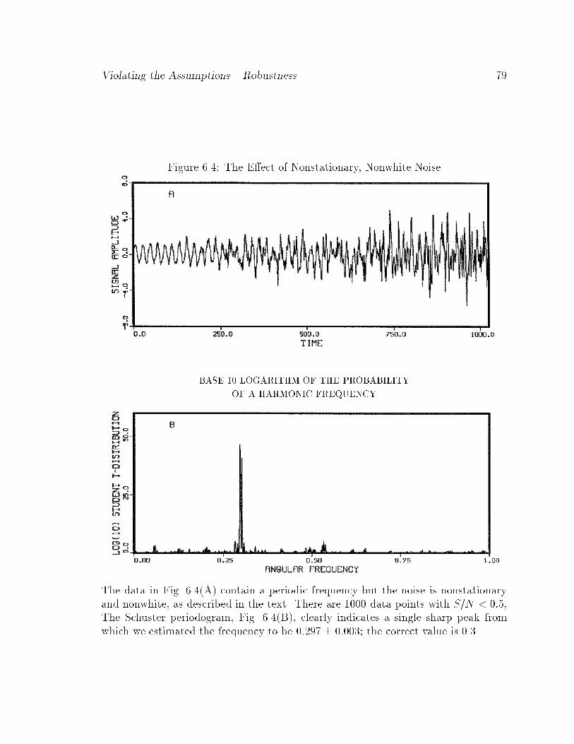
Violating the Assumptions { Robustness 79
Figure 6.4: The E�ect of Nonstationary, Nonwhite Noise
BASE 10 LOGARITHM OF THE PROBABILITY
OF A HARMONIC FREQUENCY
The data in Fig. 6.4(A) contain a periodic frequency but the noise is nonstationaryand nonwhite, as described in the text. There are 1000 data points with S=N < 0:5,The Schuster periodogram, Fig. 6.4(B), clearly indicates a single sharp peak fromwhich we estimated the frequency to be 0:297 � 0:003; the correct value is 0.3.
80 CHAPTER 6
accuracy; but the Bayesian conclusions still do not mislead us about this. Actually,
the nonstationarity, which obscures part of the data, was much more serious than the
nonwhiteness.
Amplitude modulation and other violations of the assumptions
It should be relatively clear by now what will happen when the amplitude of the
signal is not constant. For the single stationary frequency problem the su�cient
statistic is the Schuster periodogram, and we know from past experience that this
statistic is at least usable on nonstationary series with Lorentzian or Gaussian decay.
We can also say that when the amplitude modulation is completely unknown, the
single largest peak in the discrete Fourier transform is the only indication of frequen-
cies: all others are evidence but not proof. If one wishes to investigate these others
one must include some information about the amplitude modulation.
It should be equally obvious that when the signal consists of several stationary
sinusoids, the periodogram continues to work well as long as the frequencies are
reasonably well separated. But any part of the data that does not �t the model is
noise. In cases where we analyze data that contain multiple stationary frequencies
using a one-frequencymodel, all of the frequencies except the one corresponding to the
largest peak in the discrete Fourier transform are from the standpoint of probability
theory just noise { and extremely correlated, non-Gaussian noise.
All of these e�ects, and why probability theory continues to work after a fashion
in spite of them, are easily understood in terms of the intuitive picture given earlier
on page 36. We are picking the frequency so that the dot product between the data
and the model is as large as possible. In the case of the sawtooth function described
earlier, it is obvious that the \best" �t will occur when the frequency matches that
of the sawtooth, although the �t of a sawtooth to a sinusoid cannot be very good; so
probability theory will estimate the noise to be large. The same is true for harmonic
frequencies with decay; however, the estimated amplitude and phase of the signal will
not be accurate. This interpretation should also warn you that when you try to �t
a semiperiodic signal (like a Bessel oscillation) to a single sinusoidal model, the �t
will be poor. Fundamentally, the spectrum of a nonsinusoidal signal does not have a
sharp peak; and so the sharpness of the periodogram is no longer a criterion for how
well its parameters can be determined.
Nonuniform Sampling 81
6.1.5 Nonuniform Sampling
All of the analysis done in Chapters 2 through 5 is valid when the sampling inter-
vals are nonuniformly spaced. But is anything to be gained by using such a sampling
technique? Initially we might anticipate that the problem of aliasing will be signi�-
cantly reduced. Additionally, the low frequency cuto� is a function of the length of
time one samples. We will be using samples of the same duration, so we do not expect
to see any signi�cant change in the ability to detect and resolve low frequencies. But
will the ability to detect any signal be changed? Will sampling at a nonuniform rate
make it possible to estimate a frequency better? We will attempt to address all of
these concerns. But most of this will be in the form of numerical demonstrations. No
complete analytical theory exists on this subject.
Aliasing
We will address the question of aliasing �rst. To make this test as clear as possible
we have performed it without noise. The data were generated using
dj = cos([� + 0:3]tj + 1):
For the uniform sampled data tj is a simple index running from �T to T by integer
steps and 2T + 1 = 512. Except for the lack of noise and the addition of � to
the frequency this is just the example used in Fig. 6.1. Figure 6.5(A) is a plot
of this uniformly sampled series. The true frequency is 0:3 + �, but the plot has
the appearance of a frequency of only 0.3 radians per unit step. In the terminology
introduced by Tukey, this is an \alias" of the true frequency. The true frequency
is oscillating more than one full cycle for each time step measured. The nonaliased
frequencies that can be discriminated, with uniform time samples, have ranges from
0 to �=2. The periodogram of these data Fig. 6.5(B) has four peaks in the range
0 � ! � 2�: the true frequency at 0:3 + � and three aliases.
The nonuniform sampled time series Fig. 6.5(C) also has a time variable which
takes on values from �T to T . There are also 512 data points. The true frequency is
unchanged. The time variable was randomly sampled. A random number generator
with uniform distribution was used to generate 512 random numbers. These numbers
were scaled onto the proper time intervals and the simulated signal was then evaluated
at these points. No one particular region was intentionally sampled more than any

82 CHAPTER 6
Figure 6.5: Why Aliases Exist
UNIFORMLY SAMPLED SERIES SCHUSTER PERIODOGRAM
NONUNIFORMLY SAMPLED
TIME SERIES
SCHUSTER PERIODOGRAM OF
THE NONUNIFORM TIME SERIES
Aliasing is caused by uniform sampling of data. To demonstrate this we have preparedtwo sets of data: A uniformly sampled set (A), and a nonuniformly sampled set (C).The periodogram for the uniform signal, (B), contains a peak at the true frequency(0:3+�) plus three alias peaks. The periodogram of the nonuniformly sampled data,(D) has no aliases.

Nonuniform Sampling 83
other. The time series, Fig. 6.5(C) looks very di�erent from the uniformly sampled
time series. By sampling at di�erent intervals the presence of the high frequency
becomes apparent.
We then computed the periodogram for these data and have displayed it in
Fig. 6.5(D). The �rst striking feature is that the aliased frequencies (those correspond-
ing to negative frequencies as well as those due to adding � to the frequency) have
disappeared. The second feature which is apparent is that the two periodograms are
nearly the same height. Sampling at a nonuniform rate does not signi�cantly alter the
precision of the frequency estimates, provided we have the same amount of data, and
the same total sampling time. Third, the nonuniformly sampled time series has small
features in the periodogram which look very much like noise, even though we know
the signal has no noise. Small wiggles in the periodogram are not caused just by the
noise; they can also be caused by the irregular sampling times (it should be remem-
bered that these features are not relevant to the parameter estimation problem). The
answer to the �rst question: \Will aliasing go away when one uses a nonuniformly
sampled time series?" is yes.
Why aliasing is eliminated for a nonuniform time series is easily understood. Con-
sider Fig. 6.6; here we have illustrated the true frequency (solid line) and the three
alias frequencies from the previous example, Fig. 6.5. The squares mark the location
of three uniform sample points, while the circles mark the location of the nonuniform
points. Looking at Fig. 6.6 we now see aliasing in an entirely di�erent light. Probabil-
ity theory is indicating (quite rightly) that in the frequency region 0 � ! � 2� there
are four equally probable frequencies, Fig. 6.5(B), while for the nonuniformly sampled
data, probability theory is indicating that there is only one frequency consistent with
the data, Fig. 6.5(D).
Of course it must be true that the aliasing phenomenon returns for some su�ciently
high frequency. If the sampling times ftig, although nonuniform, are all integer
multiples of some small interval �t, then frequencies di�ering by 2�=�t will still be
aliased. We did one numerical test with a signal-to-noise ratio of one and the same true
frequency. We then calculated the periodogram for higher frequencies. We continued
increasing the frequency until we obtained the �rst alias. This occurred at a frequency
around 60�, almost 1.8 orders of magnitude improvement in the frequency band free
of aliasing. Even then this second large maximum was many orders of magnitude
below that at the �rst \true" frequency.

84 CHAPTER 6
Figure 6.6: Why Aliases Go Away for Nonuniformly Sampled Data
When aliases occur in a uniformly sampled time series, probability theory is stillworking correctly; indicating there is more than one frequency corresponding to the\best" estimate in the data. Suppose we have a signal cos(0:3 + �)t (solid line).For a uniformly sampled data (squares) there are four possible frequencies: ! = 0:3(dotted line), ! = � � 0:3 (dashed line), ! = 2� � 0:3 (chain dot), and the truefrequency (solid line) which pass through the uniform data (marked with squares).For nonuniformly sampled time series (marked with circles), aliases e�ectively do notoccur because only the \true" (solid line) signal passes through the nonuniformlyspaced points (circles).
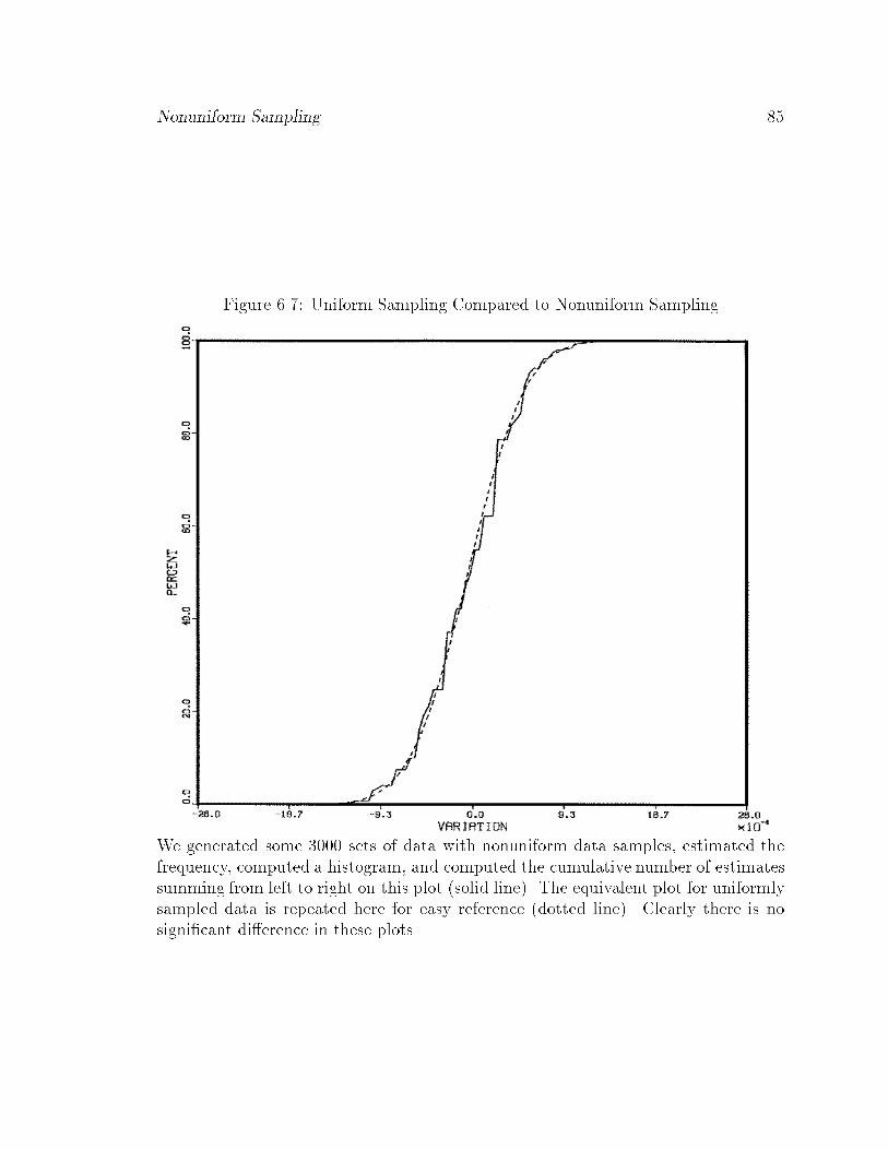
Nonuniform Sampling 85
Figure 6.7: Uniform Sampling Compared to Nonuniform Sampling
We generated some 3000 sets of data with nonuniform data samples, estimated thefrequency, computed a histogram, and computed the cumulative number of estimatessumming from left to right on this plot (solid line). The equivalent plot for uniformlysampled data is repeated here for easy reference (dotted line). Clearly there is nosigni�cant di�erence in these plots.
86 CHAPTER 6
Nonuniform Sampling and the Frequency Estimates
The second question is \Will sampling at a nonuniform rate signi�cantly change
the frequency estimate?". To answer this question we have set up a second test,
Fig. 6.7. The simulated signal is the same as that in Fig. 6.2, only now the samples are
nonuniform. We generated some 3000 samples of the data and estimated the frequency
from each. We then computed a histogram and integrated to obtain cumulative
sampling distribution of the estimates, Fig. 6.7. If nonuniform sampling improves the
frequency resolution then we would expect the cumulative distribution (solid line) to
rise faster than for the uniformly sampled case (dotted line). As one can see from this
plot, nonuniform sampling is clearly equivalent to uniform sampling when it comes
to the accuracy of the parameter estimates; moreover, nonuniform sampling improves
the high frequency resolution but does not change the frequency estimates otherwise.
Some might be disturbed by the irregular appearance of the solid line in Fig. 6.7.
This irregular behavior is simply \digitization" error in the calculation. When we
performed this calculation for the uniform case the �rst time, this same e�ect was
present. We were unsure of the cause, so we repeated the calculation forcing our
searching routines to �nd the maximum of the periodogram much more precisely.
The irregular behavior was much reduced. We did not repeat this procedure on the
nonuniformly sampled data, because it is very expensive computationally.
6.2 A Frequency with Lorentzian Decay
The simple harmonic frequency problem discussed in Chapter 2 may be generalized
easily to include Lorentzian or Gaussian decay. We assume, for this discussion, that
the decay is Lorentzian; the generalization to other types of decay will become more
obvious as we proceed. For a uniformly sampled interval the model we are considering
is
f(l) = [B1 cos(!l) +B2 sin(!l)]e��l (6:3)
where l is restricted to values (1 � l � N). We now have four parameters to estimate:
the amplitudes B1, B2; the frequency !; and the decay rate �.

The \Student t-Distribution" 87
6.2.1 The \Student t-Distribution"
The solution to this problem is a straightforward application of the general proce-
dures. The matrix gij (3.4) is given by
gij =
0BBBB@
NXl=1
cos2(!l)e�2�lNXl=1
cos!l sin!le�2�l
NXl=1
cos!l sin!le�2�lNXl=1
sin2(!l)e�2�l
1CCCCA :
This problem can be solved exactly. However, the exact solution is tedious, and
not very informative. Fortunately an approximate solution is easily obtained which
exhibits most of the important features of the full solution; and is valid in the same
sense that a discrete Fourier transform is valid. We approximate gij as follows: First
the sum over the sine squared and cosine squared terms may be approximated as
c �NXl=1
cos2(!l)e�2l� �NXl=1
sin2(!l)e�2l�
=1
2
NXl=1
[1� cos(2!l)]e�2l�
� 1
2
NXl=1
e�2l�
=1
2
"1 � e�2N�
e2� � 1
#:
(6:4)
Second, the o� diagonal terms are at most the same order as the ignored terms; these
terms are therefore ignored. Thus the matrix gij can be approximated as
gij ��c 00 c
�:
The orthonormal model functions may then be written as
H1(l) = cos(!l)e��l=pc (6:5)
H2(l) = sin(!l)e��l=pc (6:6)
The projections of the data onto the orthonormal model functions (3.13) are given by
h1 �R(!; �)p
c=
1pc
NXl=1
dl cos(!l)e��l
88 CHAPTER 6
h2 �I(!; �)p
c=
1pc
NXl=1
dl sin(!l)e��l
and the joint posterior probability of a frequency ! and a decay rate � is given by
P (!; �jD; I) /"1 � R(!; �)2 + I(!; �)2
Ncd2
# 2�N2
: (6:7)
This approximation is valid provided there are plenty of data, N � 1, and there is
no evidence of a low frequency. There is no restriction on the range of �: if � > 0 the
signal is decaying with increasing time, if � < 0 the signal is growing with increasing
time, and if � = 0 the signal is stationary. This equation is analogous to (2.8) and
reduces to (2.8) in the limit �! 0.
6.2.2 Accuracy Estimates
We derived a general estimate for the f!g parameters in Chapter 4, and we would
like to use those estimates for comparison with the single stationary frequency prob-
lem. To do this we can approximate the probability distribution P (!; �jD;�; I) by a
Gaussian as was done in Chapter 4. This may be done readily by assuming a form
of the data, and then applying Eqs. (4.9) through (4.14). From the second derivative
we may obtain the desired (mean) � (standard deviation) estimates. Approximate
second derivatives, usable with real data, may be obtained analytically as follows.
We take as the data
d(t) = B cos(!t)e��t; (6:8)
where ! is the true frequency of oscillation and � is the true decay rate. We have
assumed only a cosine component to e�ect some simpli�cations in the discussion. It
will be obvious at the end of the calculation that the result for a signal of arbitrary
phase and magnitude may be obtained by replacing the amplitude B2 by the squared
magnitude B2 ! B21 + B2
2 .
The projection of the data (6.8) onto the model functions (6.5), and (6.6) is:
h1 =B
2pc
"NXl=1
cos(! � !)le�(�+�)l +NXl=1
cos(! + !)le�(�+�)l#:
The second term is negligible compared to the �rst under the conditions we have in
mind. Likewise, the projection h2 is essentially zero compared to h1 and we have

Accuracy Estimates 89
ignored it. These sums may be done explicitly using (6.4) to obtain
h1 =B
4pc
"1 � e�2Nv
e2v � 1+1 � e�2Nu
e2u � 1
#
where
v =� + �� i(! � !)
2and u =
�+ �+ i(! � !)
2;
and i =p�1 in the above equations. Then the su�cient statistic h2 is given by:
h2 =B2
16
"e2� � 1
1� e�2N�
# "1 � e�2Nv
1� e2v+1 � e�2Nu
1� e2u
#2
The region of the parameter space we are interested in is where the unitless decay
rate is small compared to one, and exp(N�) is large compared to one. In this region
the true signal decays away in the observation time, but not before we obtain a good
representative sample of it. We are not considering the case were the decay is so slow
that the signal is nearly stationary, or so fast that the signal is gone within a small
fraction of the observation time. Within these limits the su�cient statistic h2 is
h2 � B2�
2
"� + �
(�+ �)2 + (! � !)2
#2:
The �rst derivatives of h2 evaluated at ! = ! and � = � are zero, as they should
be. The mixed second partial derivative is also zero, indicating that the presence of
decay does not (to second order) shift the location of a frequency, and this of course
explains why the discrete Fourier transform works on problems with decay. This gives
the second derivatives of h2 as
b� � � @2h2
@�2
!�=�
=B2
16�3and b! � �
@2h2
@!2
!!=!
=B2
2�3:
From these derivatives we then make the (mean) � (standard deviation) estimates of
the frequency and decay rate to obtain
(�)est = �� �pb�
and (!)est = ! � �pb!
where�pb�� 2:8��
32
jBjand
�pb!� ��
32
jBj: (6:9)
Converting to physical units, if the sampling rate is �t and � is now the true decay
rate in hertz, these accuracy estimates are
�pb�� 2:8�
jBjp�3�t Hertz and
�pb!� �
jBjp�3�t Hertz:
90 CHAPTER 6
Just as with the single frequency problem the accuracy depends on the signal-to-noise
ratio and on the amount of data. In the single frequency case the amount of data
was represented by the factor of N . Here the amount of data depends on two factors:
the true decay rate �, and the sampling time �t. The only factor the experimenter
can typically control is the sampling time �t. With a decaying signal, to improve
the accuracy of the parameter estimates one must take the data faster, thus ensuring
that the data are sampled in the region where the signal is large, or one must improve
the signal-to-noise ratio of the data.
How does this compare to the results obtained before for the simple harmonic
frequency? For a signal with N = 1000, a decay rate of � = 2Hz, B=p2� = 1, and
again taking data for 1 second gives the accuracy estimates for frequency and decay
as
(!)est = ! � 0:06 Hz and (�)est = � � 0:17 Hz:
The uncertainty in ! is 0.13Hz compared to 0:025Hz for an equivalent stationary
signal with the same signal-to-noise ratio. This is a factor of 2.4 times larger than
for a stationary sinusoid, and since the error varies like N� 32 we have e�ectively lost
all but one third of the data due to decay. When we have reached the unitless time
of t = 250 the signal is down by a factor of 12 and has all but disappeared into the
noise. Again, the results of probability theory correspond nicely to the indications of
common sense { but they are quantitative where common sense is not.
6.2.3 Example { One Frequency with Decay
To illustrate some of these points we been making, we have prepared two more
examples: �rst we will investigate the use of this probability density when the decay
mode is known and second when it is unknown.
Known method of decay
Figure 6.8 is an example of the use of the posterior probability (6.7) when the signal
is known to be harmonic with Lorentzian decay. This time series was prepared from
the following equation
dj = 0:001 + cos(0:3j + 1)e�0:01j + ej: (6:10)
The N = 512 data samples were prepared in the following manner: �rst, we generated
the data without the noise; we then computed the average of the data, and subtracted
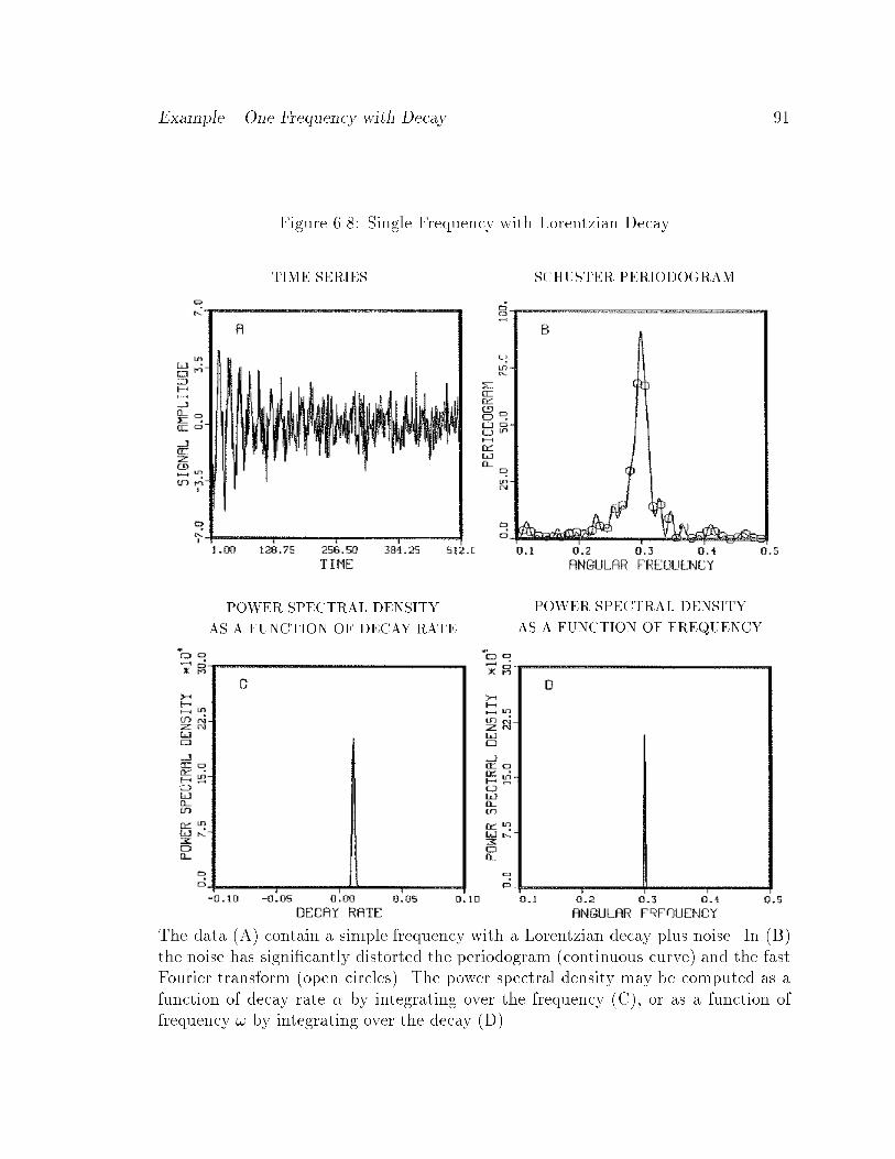
Example { One Frequency with Decay 91
Figure 6.8: Single Frequency with Lorentzian Decay
TIME SERIES SCHUSTER PERIODOGRAM
POWER SPECTRAL DENSITY
AS A FUNCTION OF DECAY RATE
POWER SPECTRAL DENSITY
AS A FUNCTION OF FREQUENCY
The data (A) contain a simple frequency with a Lorentzian decay plus noise. In (B)the noise has signi�cantly distorted the periodogram (continuous curve) and the fastFourier transform (open circles). The power spectral density may be computed as afunction of decay rate � by integrating over the frequency (C), or as a function offrequency ! by integrating over the decay (D).
92 CHAPTER 6
it from each data point, to ensure that the average of the data is zero; we then repeated
this process on the Gaussian white noise; next, we scaled the computer generated
signal by the appropriate ratio to make the signal-to-noise ratio of the data analyzed
exactly one. The time series clearly shows a small signal which rapidly decays away,
Fig. 6.8(A). Figure 6.8(B), the periodogram (continuous curve) and the fast Fourier
transform (open circles) clearly show the Lorentzian line shape. The noise is now
signi�cantly a�ecting the periodogram: the periodogram is no longer an optimum
frequency estimator.
Figures 6.8(C) and 6.8(D) contain plots of the power spectral density (4.16). In
Fig. 6.8(C) we have treated the frequency as a nuisance parameter and have inte-
grated it out numerically; as was emphasized earlier this is essentially the posterior
probability distribution for � normalized to a power level rather than to unity. In
Fig. 6.8(D) we have treated the decay as the nuisance parameter and have integrated
it out. This gives the power spectral estimate as a function of frequency.
The width of these curves is a measure of the uncertainty in the determination of
the parameters. We have determined full-width at half maximum (numerically) for
each of these and have compared these to the theoretical \best" estimates (6.9) and
�nd
(!)est = 0:2998 � 5 � 10�4 and (!)best = 0:3000 � 6 � 10�4;
(�)est = 0:0109 � 1:6 � 10�3 and (�)best = 0:0100 � 1:6 � 10�3:
The theoretical estimates and those calculated from these data are e�ectively identi-
cal.
Unknown Method of Decay
Now what e�ect does not knowing the true model have on the estimated accuracy
of these parameters? To test this we have analyzed the signal from Fig. 6.8 using
four di�erent models and have summarized the results in Table . There are several
signi�cant observations about the accuracy estimates; including a decay mode does
not signi�cantly a�ect the frequency estimates; however it does improve the accuracy
estimates for the frequency as well as the estimated standard deviation of the noise
�, but not very much.
As we had expected, the Gaussian decay does not �t the data well: it decays
away too fast, and the accuracy estimates are a little poorer. As with the single
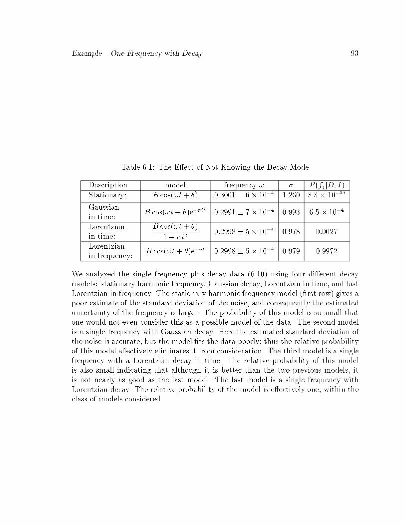
Example { One Frequency with Decay 93
Table 6.1: The E�ect of Not Knowing the Decay Mode
Description model frequency ! � P (fj jD; I)Stationary: B cos(!t+ �) 0:3001 � 6� 10�4 1.260 8:3 � 10�33
Gaussianin time:
B cos(!t+ �)e��t2
0:2991 � 7� 10�4 0.993 6:5 � 10�4
Lorentzianin time:
B cos(!t+ �)
1 + �t20:2998 � 5� 10�4 0.978 0:0027
Lorentzianin frequency:
B cos(!t+ �)e��t 0:2998 � 5� 10�4 0.979 0.9972
We analyzed the single frequency plus decay data (6.10) using four di�erent decaymodels: stationary harmonic frequency, Gaussian decay, Lorentzian in time, and lastLorentzian in frequency. The stationary harmonic frequency model (�rst row) gives apoor estimate of the standard deviation of the noise, and consequently the estimateduncertainty of the frequency is larger. The probability of this model is so small thatone would not even consider this as a possible model of the data. The second modelis a single frequency with Gaussian decay. Here the estimated standard deviation ofthe noise is accurate, but the model �ts the data poorly; thus the relative probabilityof this model e�ectively eliminates it from consideration. The third model is a singlefrequency with a Lorentzian decay in time. The relative probability of this modelis also small indicating that although it is better than the two previous models, itis not nearly as good as the last model. The last model is a single frequency withLorentzian decay. The relative probability of the model is e�ectively one, within theclass of models considered.
94 CHAPTER 6
harmonic frequency problem when we were demonstrating the e�ects of violating the
assumptions, nothing startling happens here and maybe that is the most startling
thing of all. Because it means that we do not have to know the exact models to
make signi�cant progress on analyzing the data. All we need are models which are
reasonable for the data; i.e. models which take on most of the characteristics of the
data.
The last column in this table is the relative probability of the various models (5.1).
The relative probability of the single harmonic frequencymodel, 8:3�10�33 completely
rules this model out as a possible explanation of these data. This is again not surpris-
ing: one can look at the data and see that it is decaying away. This small probability
is just a quantitative way of stating a conclusion that we draw so easily without any
probability theory. The Gaussian model �ts the data much better, 6:5 � 10�4, but
not as well as the two Lorentzian models. The Lorentzian model in time has only
about one chance in 500 of being \right" (i.e. of providing a better description of
future data than the Lorentzian in frequency). Thus probability theory can rank var-
ious models according to how well they �t the data, and discriminates easily between
models which predict only slightly di�erent data.
6.3 Two Harmonic Frequencies
We now turn our attention to the slightly more general problem of analyzing a data
set which we postulate contains two distinct harmonic frequencies. The \Student t-
distribution" represented by (3.17) is, of course, the general solution to this problem.
Unfortunately, that equation does not lend itself readily to understanding intuitively
what is in the probability distribution. In particular we would like to know the
behavior of these equations in three di�erent limits: �rst, when the frequencies are
well separated; second, when they are close but distinct; and third, when they are so
close as to be, for all practical purposes, identical. To investigate these we will solve,
approximately, the two stationary frequency problem.
6.3.1 The \Student t-Distribution"
The model equation for the two-frequency problem is a simple generalization of

The \Student t-Distribution" 95
the single-harmonic problem:
f(t) = B1 cos(!1t) +B2 cos(!2t) +B3 sin(!1t) +B4 sin(!2t):
The model functions can then be used to construct the gjk matrix. On a uniform grid
this is given by
gjk =
0BBB@c11 c12 0 0c12 c22 0 00 0 s11 s120 0 s12 s22
1CCCA
where
cjk =TX
l=�T
cos(!jl) cos(!kl) =sin(1
2N!+)
2 sin(12!+)
+sin(1
2N!�)
2 sin(12!�)
(6:11)
sjk =TX
l=�T
sin(!j l) sin(!kl) =sin(1
2N!�)
2 sin(12!�)
�sin(1
2N!+)
2 sin(12!+)
(6:12)
!+ = !j + !k; (j; k = 1 or 2)
!� = !j � !k:
The eigenvalue and eigenvector problem for gjk splits into two separate problems,
each involving 2 � 2 matrices. The eigenvalues are:
�1 =c11 + c22
2+q(c11 � c22)2 + 4c212; �2 =
c11 + c22
2�q(c11 � c22)2 + 4c212;
�3 =s11 + s22
2+q(s11 � s22)2 + 4s212; and �4 =
s11 + s22
2�q(s11 � s22)2 + 4s212:
Well Separated Frequencies
When the frequencies are well separated j!1�!2j � 2�=N , the eigenvalues reduce
to � = N=2. That is, gjk goes into N=2 times the unit matrix. Then the model
functions are e�ectively orthogonal and the su�cient statistic h2 reduces to
h2 =2
N[C(!1) + C(!2)] :
The joint posterior probability, when the variance is known, is given by
P (!1; !2jD;�; I) / exp
"C(!1) + C(!2)
�2
#: (6:13)
The problem has separated: one can estimate each of the frequencies separately. The
maximum of the two-frequency posterior probability density will be located at the
two greatest peaks in the periodogram, in agreement with the common sense usage
of the discrete Fourier transform.

96 CHAPTER 6
Two Very Close Frequencies
The labels !1, !2, etc. for the frequencies in the model are arbitrary, and accord-
ingly their joint probability density is invariant under permutations. That means,
for the two-frequency problem, there is an axis of symmetry running along the line
!1 = !2. We do not know from (6.13) what is happening along that line. This is
easily investigated: when !1 = !2 � ! the eigenvalues become
�1 = N; �2 = 0; �3 = N; �4 = 0:
The matrix gjk has two redundant eigenvalues, and the probability distribution be-
comes
P (!jD;�; I) / exp
(C(!)
�2
): (6:14)
The probability density goes smoothly into the single frequency probability distri-
bution along this axis of symmetry. Given that the two frequencies are equal, our
estimate of themwill be identical, in value and accuracy, to those of the one frequency
case. In the exact solution, the factor of two that we would have if we attempted to
use (6.13) where it is not valid, is just cancelled out.
Close But Distinct Frequencies
We have not yet addressed the posterior probability density when there are two
close but distinct frequencies. To understand this aspect of the problem we could
readily diagonalize the matrix gjk and obtain the exact solution. However, just like
the single frequency case with Lorentzian decay, this would be extremely tedious and
not very productive. Instead we derive an approximate solution which is simpler and
valid nearly everywhere if N is large. To obtain this approximate solution one needs
only to examine the matrix gjk and notice that the elements of this matrix consist of
the diagonal elements given by:
c11 =N
2+sin(N!1)
2 sin(!1)� N
2;
c22 =N
2+sin(N!2)
2 sin(!2)� N
2;
s11 =N
2� sin(N!1)
2 sin(!1)� N
2;
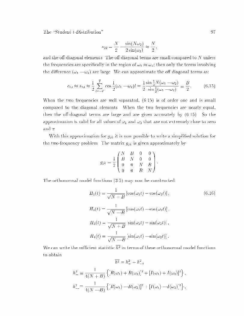
The \Student t-Distribution" 97
s22 =N
2� sin(N!2)
2 sin(!2)� N
2;
and the o�-diagonal elements. The o�-diagonal terms are small compared to N unless
the frequencies are speci�cally in the region of !1 � !2; then only the terms involving
the di�erence (!1 � !2) are large. We can approximate the o� diagonal terms as:
c12 � s12 �1
2
TXl=�T
cos1
2(!1 � !2)l =
1
2
sin 1
2N(!1 � !2)
sin 1
2(!1 � !2)
� B
2: (6:15)
When the two frequencies are well separated, (6.15) is of order one and is small
compared to the diagonal elements. When the two frequencies are nearly equal,
then the o�-diagonal terms are large and are given accurately by (6.15). So the
approximation is valid for all values of !1 and !2 that are not extremely close to zero
and �.
With this approximation for gjk it is now possible to write a simpli�ed solution for
the two-frequency problem. The matrix gjk is given approximately by
gjk =1
2
0BBB@N B 0 0B N 0 00 0 N B
0 0 B N
1CCCA :
The orthonormal model functions (3.5) may now be constructed:
H1(t) =1p
N +B[cos(!1t) + cos(!2t)] ; (6:16)
H2(t) =1p
N �B[cos(!1t)� cos(!2t)] ;
H3(t) =1p
N +B[sin(!1t) + sin(!2t)] ;
H4(t) =1p
N �B[sin(!1t)� sin(!2t)] :
We can write the su�cient statistic h2 in terms of these orthonormal model functions
to obtain
h2 = h2+ + h2�;
h2+ �1
4(N +B)
n[R(!1) +R(!2)]
2 + [I(!1) + I(!2)]2o;
h2� �1
4(N �B)
n[R(!1)�R(!2)]
2 + [I(!1)� I(!2)]2o;
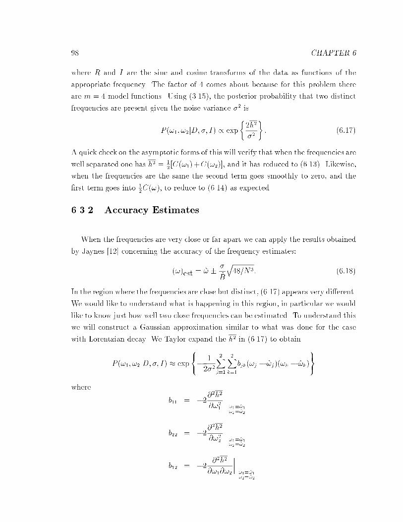
98 CHAPTER 6
where R and I are the sine and cosine transforms of the data as functions of the
appropriate frequency. The factor of 4 comes about because for this problem there
are m = 4 model functions. Using (3.15), the posterior probability that two distinct
frequencies are present given the noise variance �2 is
P (!1; !2jD;�; I) / exp
(2h2
�2
): (6:17)
A quick check on the asymptotic forms of this will verify that when the frequencies are
well separated one has h2 = 1
2[C(!1)+C(!2)], and it has reduced to (6.13). Likewise,
when the frequencies are the same the second term goes smoothly to zero, and the
�rst term goes into 1
2C(!), to reduce to (6.14) as expected.
6.3.2 Accuracy Estimates
When the frequencies are very close or far apart we can apply the results obtained
by Jaynes [12] concerning the accuracy of the frequency estimates:
(!)est = ! � �
B
q48=N3: (6:18)
In the region where the frequencies are close but distinct, (6.17) appears very di�erent.
We would like to understand what is happening in this region, in particular we would
like to know just how well two close frequencies can be estimated. To understand this
we will construct a Gaussian approximation similar to what was done for the case
with Lorentzian decay. We Taylor expand the h2 in (6.17) to obtain
P (!1; !2jD;�; I) � exp
8<:� 1
2�2
2Xj=1
2Xk=1
bjk(!j � !j)(!k � !k)
9=;
where
b11 = �2@2h2
@!21
����!1=!1!2=!2
b22 = �2@2h2
@!22
����!1=!1!2=!2
b12 = �2 @2h2
@!1@!2
����!1=!1!2=!2
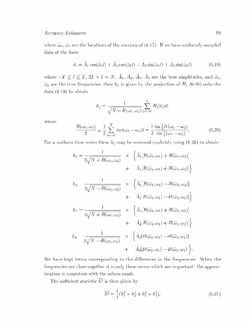
Accuracy Estimates 99
where !1, !2 are the locations of the maxima of (6.17). If we have uniformly sampled
data of the form
dl = A1 cos(!1l) + A2 cos(!2l) + A3 sin(!1l) + A4 sin(!2l) (6:19)
where �T � l � T , 2T + 1 = N , A1, A2, A3, A4 are the true amplitudes, and !1,
!2 are the true frequencies, then hj is given by the projection of Hj (6.16) onto the
data (6.19) to obtain
hj =1q
N +B(!1; !2)
TXl=�T
Hj(tl)dl
whereB(!1; !2)
2� 1
2
TXl=�T
cos(!1 � !2)l =1
2
sin 1
2N(!1 � !2)
sin 1
2(!1 � !2)
: (6:20)
For a uniform time series these hj may be summed explicitly using (6.20) to obtain
h1 =1
2qN + B(!1; !2)
��A1[B(!1; !1) +B(!1; !2)]
+ A2[B(!2; !1) +B(!2; !2)]�
h2 =1
2qN �B(!1; !2)
��A1[B(!1; !1)�B(!1; !2)]
+ A2[B(!2; !1)�B(!2; !2)]�
h3 =1
2qN + B(!1; !2)
��A3[B(!1; !1) +B(!1; !2)]
+ A4[B(!2; !1) +B(!2; !2)]�
h4 =1
2qN �B(!1; !2)
��A3[B(!1; !1)�B(!1; !2)]
+ A4[B(!2; !1)�B(!2; !2)]�:
We have kept terms corresponding to the di�erences in the frequencies. When the
frequencies are close together it is only these terms which are important: the approx-
imation is consistent with the others made.
The su�cient statistic h2 is then given by
h2 =1
4(h21 + h22 + h23 + h24): (6:21)
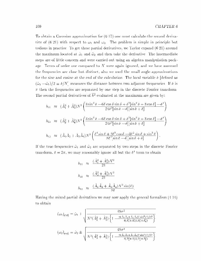
100 CHAPTER 6
To obtain a Gaussian approximation for (6.17) one must calculate the second deriva-
tive of (6.21) with respect to !1 and !2. The problem is simple in principle but
tedious in practice. To get these partial derivatives, we Taylor expand (6.21) around
the maximum located at !1 and !2 and then take the derivative. The intermediate
steps are of little concern and were carried out using an algebra manipulation pack-
age. Terms of order one compared to N were again ignored, and we have assumed
the frequencies are close but distinct, also we used the small angle approximations
for the sine and cosine at the end of the calculation. The local variable � [de�ned as
(!2 � !1)=2 � �=N ] measures the distance between two adjacent frequencies. If � is
� then the frequencies are separated by one step in the discrete Fourier transform.
The second partial derivatives of h2 evaluated at the maximum are given by:
b11 � (A21 + A2
3)N3
3 sin2 � � 6� cos � sin � + �2[sin2 � + 3 cos �]� �4
24�3[sin � � �][sin� + �]
!
b22 � (A22 + A2
4)N3
3 sin2 � � 6� cos � sin � + �2[sin2 � + 3 cos �]� �4
24�3[sin � � �][sin� + �]
!
b12 � (A1A2 + A3A4)N3
�4 sin � + 2�3 cos � � 3�2 sin � + sin3 �
8�3[sin � � �][sin � + �]
!:
If the true frequencies !1 and !2 are separated by two steps in the discrete Fourier
transform, � = 2�, we may reasonably ignore all but the �4 term to obtain
b11 � (A21 + A2
3)N3
24
b22 � (A22 + A2
4)N3
24
b12 � (A1A2 + A3A4)N3 sin(�)
8� :
Having the mixed partial derivatives we may now apply the general formalism (4.14)
to obtain
(!1)est = !1 �vuuut 48�2
N3(A21 + A2
3)�1 � 9(A1A2+A3 A4)2 sin
2(�)=�2
4(A21+A
23)(A
22+A
24)
�
(!2)est = !2 �vuuut 48�2
N3(A22 + A2
4)�1 � 9(A1A2+A3 A4)2 sin
2(�)=�2
4(A21+A
23)(A
22+A
24)
�
More Accuracy Estimates 101
The accuracy estimates reduce to (6.18) when the frequencies are well separated.
When the frequencies have approximately the same amplitudes and � is order of
2� (the frequencies are separated by two steps in the fast Fourier transform) the
interaction term is down by approximately 1/36; and one expects the estimates to be
nearly the same as those for a single frequency. Probability theory indicates that two
frequencies which are as close together as two steps in a discrete Fourier transform
do not interfere with each other in any signi�cant way. Also note the appearance of
the sinc function in the above estimates. When the frequencies are separated by a
Nyquist step (j!1 � !2j = 2�=N) the frequencies cannot interfere with each other.
Although this is a little surprising at �rst sight, a moment's thought will convince
one that when the frequencies are separated by 2�=N the sampled vectors are exactly
orthogonal to each other and because we are e�ectively taking dot products between
the model and the data, of course they cannot interfere with each other.
6.3.3 More Accuracy Estimates
To better understand the maximum theoretical accuracy with which two frequen-
cies can be estimated we have prepared Table 6.2. To make these estimates compara-
ble to those obtained in Chapter 2 we have again assumed N = 1000 data points and
� = 1. There are three regions of interest: when the frequency separation is small
compared to a single step in the discrete Fourier transform; when the separation is
of order one step; and when the separation is large. Additionally we would like to
understand the behavior when the signals are of the same amplitude, when one signal
is slightly larger than the other, and when one signal is much larger than the other.
When we prepared this table we used the joint posterior probability of two frequen-
cies (3.16) assuming the variance �2 known. The estimates obtained are the \best" in
the sense that in a real data set with � = 1, and N = 1000 data points the accuracy
estimates one obtains will be, nearly always, slightly worse than those contained in
table 6.2.
The three values of (!1 �!2) examined correspond to � = 1=4, � = 4, and � = 16:
roughly these correspond to frequency separations of 0.07, 0.3, and 5.1 Hz. We held
the squared magnitude of one signal constant, and the second is either 1, 4 or 128
times larger.
When the separation frequency is 0.07 Hz the frequencies are indistinguishable.
The smaller component cannot be estimated accurately. As the magnitude of the

102 CHAPTER 6
Table 6.2: Two Frequency Accuracy EstimatespB22+B
24p
B21+B
23
�f = 0:07 Hz �f = 0:3 Hz �f = 5:1 Hz
�f1 Hz �f2 Hz �f1 Hz �f2 Hz �f1 Hz �f2 Hz1 �0:091 �0:091 �0:027 �0:027 �0:025 �0:0254 �0:091 �0:088 �0:027 �0:013 �0:025 �0:012128 �0:091 �0:034 �0:025 �0:0024 �0:025 �0:0022
We ran a number of simulations to determine how well two frequencies could be determined.
In column 1 the two frequencies are separated by only 0.07 Hz and cannot be resolved.
In column 2 the separation frequency is now 0.3 Hz and the resolution is approximately
0.0025 Hz for each of the three amplitudes tested. We would have to move one of the
frequencies by 11 standard deviations before they would overlap each other. In column 3
the frequencies are separated by 5.1 Hz and we would have to move one of the frequencies
by 200 standard deviations before they overlapped.
second signal increases, the estimated accuracy of the second signal becomes better
as one's intuition would suppose it should (the signal looks more and more like one
frequency). But even at 128:1 probability theory still senses that all is not quite
right for a single frequency, and gives an accuracy estimate wider than for a true
one frequency signal. However, for very close frequencies the true resolving power is
conveyed only by the two-dimensional plot like Fig. 6.10 below; not by the numbers
in Table 6.2.
When the separation frequency is 0.3 Hz or about one step in the discrete Fourier
transform, the accuracy estimates indicate that the two frequencies are well resolved.
By this we mean one of the frequencies would have to be moved by 11 standard devi-
ations before it would be confounded with the other (two parameters are said to be
confounded when probability theory cannot distinguish their separate values). This is
true for all sample signals in the table; it does, however, improve with increasing am-
plitude. According to probability theory, when two frequencies are as close together
as one Nyquist step in the discrete Fourier transform, those frequencies are clearly
resolvable by many standard deviations even at S=N = 1; the Rayleigh criterion is
far surpassed.
When the separation frequency is 5.1Hz, the accuracy estimates determine both
frequencies slightly better. Additionally, the accuracy estimates for the smaller fre-
quency are essentially 0.025Hz which is the same as the estimate for a single harmonic

The Power Spectral Density 103
frequency that we found previously (2.12). Examining Table 6.2 more carefully, we
see that when the frequencies are separated by even a single step in the discrete
Fourier transform, the accuracy estimates are essentially those for the single harmonic
frequencies. The ability to estimate two close frequencies accurately is essentially in-
dependent of the separation frequency, as long as it is greater than or approximately
equal to one step in the discrete Fourier transform!
6.3.4 The Power Spectral Density
The power spectral density (4.16) speci�cally assumed there were no confounded
parameters. The exchange symmetry, in the two-harmonic frequency problem, en-
sures there are two equally probable maxima. We must generalize (4.16) to account
for these. The generalization is straightforward. We have from (4.16)
p(f!g) � 4h2P (f!gjD; h�2i; I)R
df!gP (f!gjD; h�2i; I) : (6:22)
The generalization is in the approximating of P (f!gjD; h�2i; I). Suppose for simplic-
ity that the two frequencies are well separated and the variance �2 is known; then
the matrix bjk becomes
bjk = �m2
@2h2
@!2j
�jk:
Which gives
P (f!gjD; h�2i; I)Zdf!gP (f!gjD; h�2i; I)
�
b112�h�2i
b222�h�2i
!12
� exp
(� b11
2h�2i (!1 � !1)2 �b22
2h�2i(!2 � !2)2)
when expanded around !1 � !1, !2 � !2, and
P (f!gjD; h�2i; I)Zdf!gP (f!gjD; h�2i; I)
�
b11
2�h�2ib22
2�h�2i
!12
� exp
(� b11
2h�2i (!1 � !2)2 �b22
2h�2i(!2 � !1)2)
when we expand around the other maximum. But to be consistent we must retain
the same symmetries in the approximation to the probability density as it originally

104 CHAPTER 6
possessed: the approximation which is valid everywhere is
P (f!gjD; h�2i; I)Zdf!gP (f!gjD; h�2i; I)
� 1
2
b11
2�h�2ib22
2�h�2i
! 12
��exp
(� b11
2h�2i(!1 � !1)2 � b22
2h�2i(!2 � !2)2
)
+ exp
(� b11
2h�2i (!1 � !2)2 � b22
2h�2i(!2 � !1)2
)�
The factor of 1/2 comes about because there are two equally probable maxima. The
power spectral density is a function of both !1 and !2, but we wish to plot it as
a function of only one variable !. We can do this by integrating out the nuisance
parameter (in this case one of the two frequencies). From symmetry, it cannot matter
which frequency we choose to eliminate. We choose to integrate out !1 and to relabel
!2 as !. Performing this integration we obtain
p(!) � 2h2(!2; !)
sb11
2�h�2i exp�� b11
2h�2i(!1 � !)2�
+ 2h2(!1; !)
sb22
2�h�2i exp�� b22
2h�2i(!2 � !)2�
and using the fact that
h2(!1; !2) = h2(!2; !1) = C(!1) + C(!2)
we have
p(!) � 2[C(!1) + C(!2)]�s
b11
2�h�2i exp�� b11
2h�2i(!1 � !)2�
+
sb22
2�h�2i exp�� b22
2h�2i(!2 � !)2��:
We see now just what that exchange symmetry is doing: The power spectral density
conveys information about the total energy carried by the signal, and about the
accuracy of each line, but the two terms have equal areas; it contains no information
about how much energy is carried in each line. That is not too surprising; after all
we de�ned the power spectral density as the total energy carried by the signal per
unit f!g. That is typically what one is interested in for an arbitrary model function.

Example { Two Harmonic Frequencies 105
However, the multiple frequency problem is unique in that one is typically interested
in the power carried by each line; not the total power carried by the signal. This is not
really a well de�ned problem in the sense that as two lines become closer and closer
together the frequencies are no longer orthogonal and power is shared between them.
The problem becomes even worse when one considers nonstationary frequencies. We
will later de�ne a line spectral density which will give information about the power
carried by one line when there are multiple well separated lines in the spectrum.
6.3.5 Example { Two Harmonic Frequencies
To illustrate some of the points we have been making about the two-frequency
probability density (6.17) we prepared a simple example, Fig. 6.9. This example was
prepared from the following equation
di = cos(0:3i+ 1) + cos(0:307i + 2) + ei
where ei has variance one and the index runs over the symmetric time interval
(�255:5 � i � 255:5) by unit steps. This time series, Fig. 6.9(A), has two sim-
ple harmonic frequencies separated by approximately 0.6 steps in the discrete Fourier
transform. One step corresponds to j!1 � !2j � 2�=512 = 0:012.
From looking at the raw time series one might just barely guess that there is more
going on than a simple harmonic frequency plus noise, because the oscillation ampli-
tude seems to vary slightly. If we were to guess that there are two close frequencies,
then by examining the data one can guess that the di�erence between these two fre-
quencies is not more than one cycle over the entire time interval. If the frequencies
were separated by more than this we would expect to see beats in the data. If there
are two frequencies, the second frequency must be within 0:012 of the �rst (in dimen-
sionless units). This is in the region where the frequency estimates are almost but
not quite confounded.
Now Fig. 6.9(B) the periodogram (continuous curve) and the fast Fourier transform
(open circles) show only a single peak. The single frequency model has estimated a
frequency which is essentially the average of the two. Yet the two frequency posterior
probability density Fig. 6.10 shows two well resolved, symmetrical maxima. Thus
the inclusion of just this one simple additional fact { that the signal may have two
frequencies { has greatly enhanced our ability to detect the two signals. Prior infor-
mation, even when it is only qualitative, can have a major e�ect on the quantitative
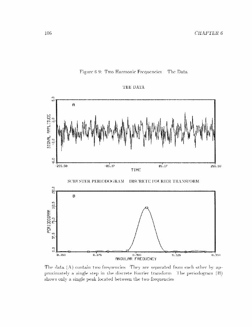
106 CHAPTER 6
Figure 6.9: Two Harmonic Frequencies { The Data
THE DATA
SCHUSTER PERIODOGRAM { DISCRETE FOURIER TRANSFORM
The data (A) contain two frequencies. They are separated from each other by ap-proximately a single step in the discrete Fourier transform. The periodogram (B)shows only a single peak located between the two frequencies.

Example { Two Harmonic Frequencies 107
Figure 6.10: Posterior Probability density of Two Harmonic Frequencies
This is a fully normalized posterior probability density of two harmonic frequenciesin the data, Fig. 6.9. The two-frequency probability density clearly indicates thepresence of two frequencies. The posterior odds ratio prefers the two-frequency modelby 107 to 1.
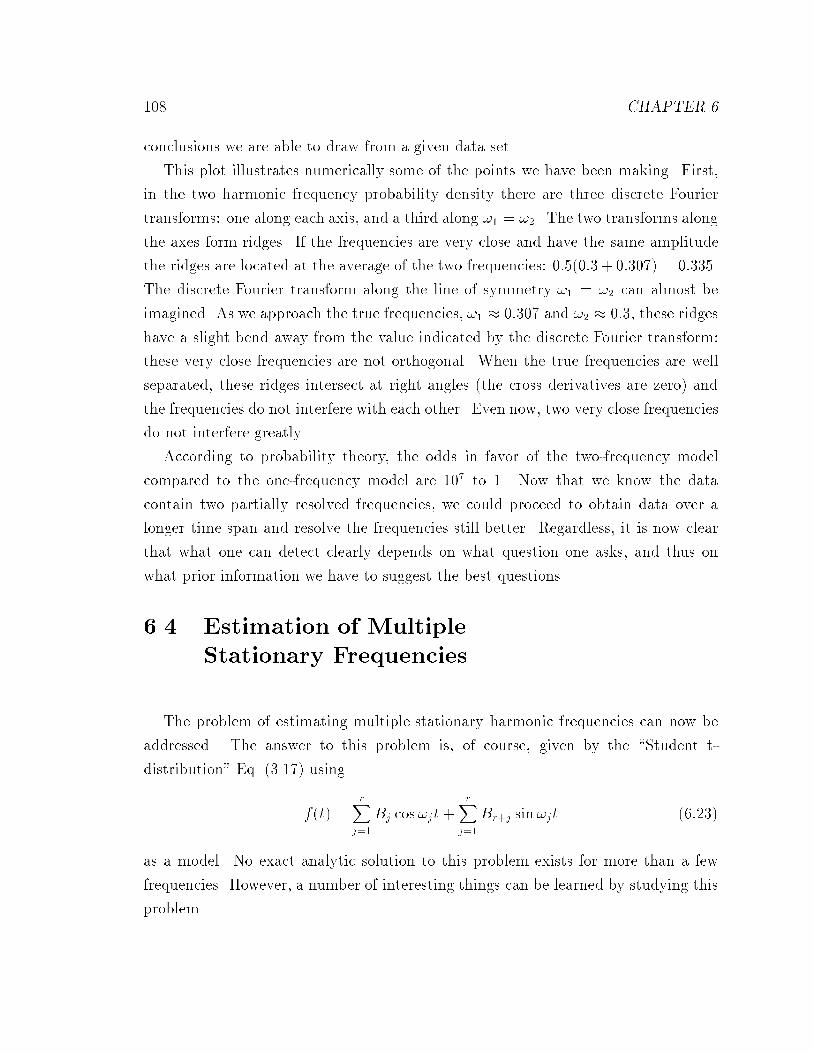
108 CHAPTER 6
conclusions we are able to draw from a given data set.
This plot illustrates numerically some of the points we have been making. First,
in the two harmonic frequency probability density there are three discrete Fourier
transforms: one along each axis, and a third along !1 = !2. The two transforms along
the axes form ridges. If the frequencies are very close and have the same amplitude
the ridges are located at the average of the two frequencies: 0:5(0:3+ 0:307) = 0:335.
The discrete Fourier transform along the line of symmetry !1 = !2 can almost be
imagined. As we approach the true frequencies, !1 � 0:307 and !2 � 0:3, these ridges
have a slight bend away from the value indicated by the discrete Fourier transform:
these very close frequencies are not orthogonal. When the true frequencies are well
separated, these ridges intersect at right angles (the cross derivatives are zero) and
the frequencies do not interfere with each other. Even now, two very close frequencies
do not interfere greatly.
According to probability theory, the odds in favor of the two-frequency model
compared to the one-frequency model are 107 to 1. Now that we know the data
contain two partially resolved frequencies, we could proceed to obtain data over a
longer time span and resolve the frequencies still better. Regardless, it is now clear
that what one can detect clearly depends on what question one asks, and thus on
what prior information we have to suggest the best questions.
6.4 Estimation of Multiple
Stationary Frequencies
The problem of estimating multiple stationary harmonic frequencies can now be
addressed. The answer to this problem is, of course, given by the \Student t-
distribution" Eq. (3.17) using
f(t) =rX
j=1
Bj cos!jt+rX
j=1
Br+j sin!jt (6:23)
as a model. No exact analytic solution to this problem exists for more than a few
frequencies. However, a number of interesting things can be learned by studying this
problem.
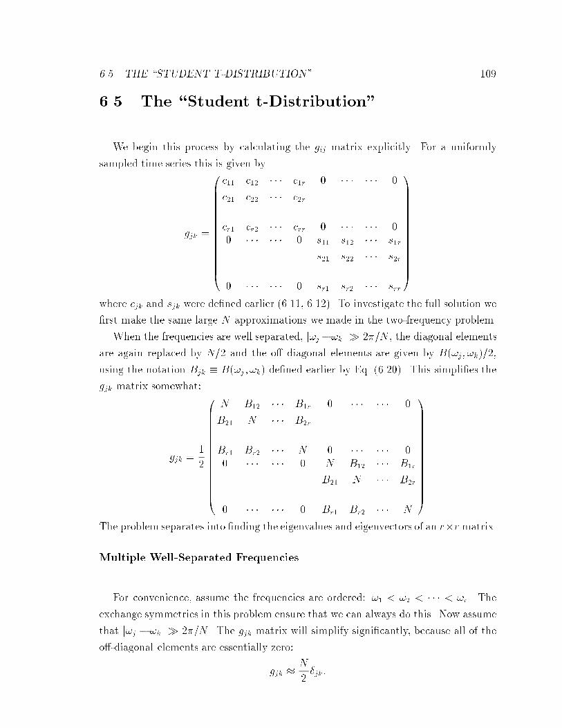
6.5. THE \STUDENT T-DISTRIBUTION" 109
6.5 The \Student t-Distribution"
We begin this process by calculating the gij matrix explicitly. For a uniformly
sampled time series this is given by
gjk =
0BBBBBBBBBBBBBBB@
c11 c12 � � � c1r 0 � � � � � � 0
c21 c22 � � � c2r...
......
......
.... . .
......
......
...cr1 cr2 � � � crr 0 � � � � � � 00 � � � � � � 0 s11 s12 � � � s1r...
......
... s21 s22 � � � s2r...
......
......
.... . .
...0 � � � � � � 0 sr1 sr2 � � � srr
1CCCCCCCCCCCCCCCA
where cjk and sjk were de�ned earlier (6.11, 6.12). To investigate the full solution we
�rst make the same large N approximations we made in the two-frequency problem.
When the frequencies are well separated, j!j�!kj � 2�=N , the diagonal elements
are again replaced by N=2 and the o� diagonal elements are given by B(!j; !k)=2,
using the notation Bjk � B(!j ; !k) de�ned earlier by Eq. (6.20). This simpli�es the
gjk matrix somewhat:
gjk =1
2
0BBBBBBBBBBBBBBB@
N B12 � � � B1r 0 � � � � � � 0
B21 N � � � B2r
......
......
......
. . ....
......
......
Br1 Br2 � � � N 0 � � � � � � 00 � � � � � � 0 N B12 � � � B1r...
......
... B21 N � � � B2r...
......
......
.... . .
...0 � � � � � � 0 Br1 Br2 � � � N
1CCCCCCCCCCCCCCCA
The problem separates into �nding the eigenvalues and eigenvectors of an r�r matrix.
Multiple Well-Separated Frequencies
For convenience, assume the frequencies are ordered: !1 < !2 < � � � < !r. The
exchange symmetries in this problem ensure that we can always do this. Now assume
that j!j � !kj � 2�=N . The gjk matrix will simplify signi�cantly, because all of the
o�-diagonal elements are essentially zero:
gjk �N
2�jk:
110 CHAPTER 6
The problem has separated completely, and the joint posterior probability of multiple
harmonic frequencies when the variance is known is given by
P (!1; � � � ; !rjD�; I) / exp
8<:
rXj=1
C(!j)
�2
9=; :
This result was �rst found by Jaynes [12]. The estimated frequencies are the r largest
peaks in the discrete Fourier transform, again in agreement with common sense. Of
course, the accuracy estimates of the frequencies are those obtained from the single
harmonic frequency problem.
If one were to estimate the accuracy from multiple frequency data using a single-
frequency model, the answers would not be the same; the estimated noise variance �2
would be far greater, because multiple-frequency data will not �t a single-frequency
model. Thus in realistic cases where the noise variance �2 must be estimated from the
data, it is essential to use the estimated variance from the multiple-frequency model
even when the frequencies are well separated.
The results from this section let us see the discrete Fourier transform in yet an-
other way: the discrete Fourier transform is a su�cient statistic for the estimation
of multiple-well separated harmonic frequencies. P. Whittle [29] derived the peri-
odogram from the principle of maximum likelihood in 1954 and stated that \: : : in
practice the periodogram presents a wildly irregular appearance, suggesting little or
nothing to the eye." It now appears that this depends on the condition of the brain
behind that eye; after a little Bayesian education, a periodogram suggests a great deal
to the eye because one knows where to look. When the frequencies are well separated,
it is only the very largest peaks in the periodogram that are important for frequency
estimation. The common practice of taking the log of the periodogram is just about
the worst thing one could do, because it accents the noise and suppresses information
about the frequencies.
Two Close Frequencies
Now assume that the �rst two frequencies are close together: j!1 - !2j � 2�=N .
Then the o� diagonal term B12 is not small. But by assumption all the remaining o�-
diagonal terms are negligible. The problem separates into a two-frequency problem
for the close frequencies and r � 1 one-frequency problems. A feasible procedure for
estimating multiple harmonic frequencies is now clear. We calculate the probability
Example { Multiple Stationary Frequencies 111
of a single harmonic frequency in the data. We take the single largest peak from the
data and we examine it with a two-frequency model. If there is any evidence of two
frequencies, we will obtain a better �t; if not the frequencies will confound with each
other. Now generate the best model function from the estimated parameters (either
a one or two-frequency model) and subtract it from the data. The di�erence is the
residual signal which must be analyzed further.
What we are contemplating here is, in spirit, what an economist would call de-
trending (i.e. estimating a trend and then subtracting it from the data). Normally
this is a bad thing to do, because the trend and the signal of interest are not orthog-
onal. We can do this here because the orthogonality properties of multiple harmonic
model functions ensures that the error is small. But, we stress, it is only the special
properties of the sine and cosine functions that make this possible.
Next we examine the residual signal using the same procedure. We compute the
posterior probability of a frequency in the residuals and examine the largest peak for
two frequencies. We repeat the entire procedure until we have reduced the residuals
to noise (i.e. until they exhibit no visible regularity). Determining the stopping place
is not generally a problem, but if there are many small signals present it will be
necessary to use the procedures developed in Chapter 5 to determine the total number
of frequencies present. We stress again that this procedure is only applicable to the
multiple stationary frequency problem and then only because of the special properties
of the sine and cosine functions. Even here, if there is evidence of multiple close
frequencies it will be necessary to use the estimates obtained from this procedure as
initial estimates for a full multiple-frequency analysis on the data.
6.5.1 Example { Multiple Stationary Frequencies
To illustrate some of the points we have been making we have prepared a sim-
ple example of a stationary signal with multiple harmonic frequencies. This simple
example was prepared from
f(t) = cos(0:1i+ 1) + 2 cos(0:15i+ 2) + 5 cos(0:3i+ 3)+ 2 cos(0:31i+ 4) + 3 cos(1i+ 5) + ei
and shown in Fig. 6.11(A), where ei has unit variance and there are N = 512 data
points. The periodogram Fig. 6.11(B) resolves the four well-separated frequencies and
then hints that the frequency near 0.3 could be two frequencies. To estimate these
frequencies we simply postulated a �ve-frequency model and used the estimates from
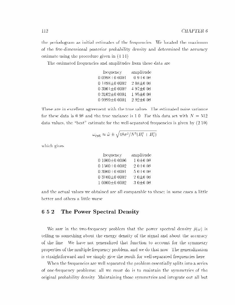
112 CHAPTER 6
the periodogram as initial estimates of the frequencies. We located the maximum
of the �ve-dimensional posterior probability density and determined the accuracy
estimate using the procedure given in (4.14).
The estimated frequencies and amplitudes from these data are
frequency amplitude0.0998�0.0001 0.9�0.080.1498�0.0002 2.08�0.080.3001�0.0002 4.97�0.080.3102�0.0001 1.95�0.080.9999�0.0001 2.92�0.08
These are in excellent agreement with the true values. The estimated noise variance
for these data is 0.98 and the true variance is 1.0. For this data set with N = 512
data values, the \best" estimate for the well-separated frequencies is given by (2.10)
!est � ! �q48�2=N3(B2
1 +B22)
which gives
frequency amplitude0.1000�0.0006 1.0�0.080.1500�0.0002 2.0�0.080.3000�0.0001 5.0�0.080.3100�0.0002 2.0�0.081.0000�0.0002 3.0�0.08
and the actual values we obtained are all comparable to these: in some cases a little
better and others a little worse.
6.5.2 The Power Spectral Density
We saw in the two-frequency problem that the power spectral density p(!) is
telling us something about the energy density of the signal and about the accuracy
of the line. We have not generalized that function to account for the symmetry
properties of the multiple frequency problem, and we do that now. The generalization
is straightforward and we simply give the result for well-separated frequencies here.
When the frequencies are well separated the problem essentially splits into a series
of one-frequency problems: all we must do is to maintain the symmetries of the
original probability density. Maintaining those symmetries and integrate out all but

The Power Spectral Density 113
Figure 6.11: Multiple Harmonic Frequencies
THE DATA SCHUSTER PERIODOGRAM
THE POWER SPECTRAL DENSITY LINE POWER SPECTRAL DENSITY
The data (A) contain �ve frequencies. Three of the �ve are well separated. TheSchuster periodogram (B) resolves the three well-separated frequencies, but one can-not tell if the peak near ! = 0:3 is one or two frequencies. The power spectral densityp(!) (C) clearly separates all �ve frequencies while the height is indicative of the res-olution. The height of the line power spectral density (D) is indicative of the energycarried by the line.
114 CHAPTER 6
one frequency, the power spectral density may be approximated as
p(!) � 2
24�2 +
rXj=1
C(!j)
35 rXk=1
"bkk
2��2
# 12
exp
(�bkk(!k � !)2
2�2
):
As was stressed earlier this function expresses information about the total energy
carried by the signal and about the accuracy of each line, but nothing about the
power carried by one line. After the fact this is not too surprising: after all, we asked
a question about the total energy carried by the signal, and not a question about the
power carried by one line. If we wish information about the power carried by one
line, we must ask a question about one line, and we do that in the next subsection.
First we illustrate the generalized power spectral density with a simple example. In
addition to determining the frequencies in the previous example we have plotted the
power spectral density in Fig. 6.11(C). We see from (C) that the �ve frequencies have
been well resolved by the \Student t-distribution": the widths of the lines from (C)
are indications of how well the lines have been determined from the data while the
integral over all lines is the total energy carried by the signal in the observation time.
6.5.3 The Line Power Spectral Density
We would like to plot a power spectral density that is an indication of the power
carried by the individual spectral lines. This is easily done simply by de�ning the
appropriate spectral density. Here we de�ne a line power spectral density S(!) as
the posterior expected value of the energy carried by one sinusoidal component of the
signal in the frequency range d!. This is given by
S(!) =N
2
Z(B2
1 +B21+r)P (fBg; f!gj�;D; I)dB1 � � � dBmd!2 � � � d!r
=2
r
h�2 + C(!)
i rXk=1
"bkk
2��2
# 12
exp
(�bkk(!k � !)2
2�2
)
where we have performed the integrals over all but the �rst frequency. We have
relabeled !1 as !. When we computed this expectation value we used the amplitudes
for frequency !1 however, the exchange symmetries in this problem ensure we will
obtain the same result whichever one we chose to leave behind. This is essentially
just the marginal posterior probability density normalized to the power carried by
one spectral line. The integral over ! will give the total energy carried by all of the
spectral lines, and in this approximation each line contributes its total energy to the
6.6. MULTIPLE NONSTATIONARY FREQUENCY ESTIMATION 115
integral. We have included an example of this in the multiple frequency example
given earlier see Fig. 6.11(D). In this �gure the lines are normalized to a power level,
the heights are indications of the total energy carried by a line, and the width is an
indication of the accuracy of the estimates.
6.6 Multiple Nonstationary Frequency Estimation
The problem of multiple nonstationary frequencies is easily addressed using the
\Student t-distribution" (3.17). As with the multiple stationary frequency estimation
problem, an analytic solution is not feasible for more than a few frequencies. However,
we already know that this problem separates. If it did not, the discrete Fourier
transform would not be useful on this problem; and it is.
The way to handle this problem is to apply the \Student t-distribution" numeri-
cally. One can apply the single-frequency-plus-decay model when the nonstationary
frequencies are well separated, and then use more complex models where needed. The
numerical procedure to use is to calculate the discrete Fourier transform of the data,
and from it compute the logarithm of the probability of a single harmonic frequency.
Then set up a nonstationary frequency model using the single best frequency from
the discrete Fourier transform. Locate the maximum of the probability density and
then compute the residuals. These residuals are essentially what probability theory
is calling the noise. Repeat the Fourier transform step on the residuals. If there are
additional frequencies in the data, repeat the process using two, three, � � �, frequenciesmodel until all frequencies have been accounted for. Of course, one can save time here
by starting with an initial model that has the same number of well-separated peaks
as are in the Fourier transform of the data. But care must be taken; if these signals
are decaying, one must supply reasonable estimates for the decay rates and this can
be very di�cult.
When applying this procedure, there is no need to check to see if any of the peaks
have multiple frequencies. Later passes through the procedure will resolve double
structure. If any of the peaks has multiple frequencies, then when one �ts the main
peak not all of the signal will be removed, and on some later cycle through the
procedure the second frequency will be the largest remaining e�ect in the data and
the procedure will pick it out. The procedure works so well and the e�ects are so
striking, that an example is needed. We give this example in the next chapter.

116 CHAPTER 6
Chapter 7
APPLICATIONS
Perhaps the greatest test of any theory is not so much how it was derived, but
how it works. Here we apply the theory as developed in the preceding chapters to a
number of speci�c examples including: NMR signals, economic time series, and Wolf's
relative sunspot numbers. Also, we examine how multiple measurements a�ect the
analysis.
7.1 NMR Time Series
NMR provides an excellent example of how the introduction of modern computers
has revolutionized a branch of science. With the aid of computers more data can be
taken and summarized into a useful form faster than has ever been possible before.
The standard way to analyze an NMR experiment is to obtain a quadrature data
set, with two separate measurements, 90� out of phase with each other, and to do
a complex Fourier transform on these data [30]. The global phase of the discrete
complex transform is adjusted until the real part (called an absorption spectrum)
is as symmetric as possible. The frequencies and decay rates are then estimated
from the absorption spectrum. There are, of course, good physical reasons why the
absorption spectrum of the \true signal" is important to physicists. However, as
we have emphasized repeatedly since Chapter 2, the discrete Fourier transform is an
optimal frequency estimator only when a single simple harmonic frequency is present,
and there are no conditions known to the author under which an absorption spectrum
will give optimal frequency estimates.
We will apply the procedures developed in the previous sections to a time series
117
118 CHAPTER 7
from a real NMR experiment, and contrast our analysis to the one done using the
absorption spectrum. The NMR data used are of a free-induction decay [31], Fig. 7.1.
The sample contained a mixture of 63% liquid Hydrogen-Deuterium (HD) and Deu-
terium (D2) at 20:2�K. The sample was excited with a 55MHz pulse, and its response
was observed using a standard mixer-modulation technique. The resulting signal is
in the audio range where it has several oscillations at about 100Hz. The data were
sampled at �t = 0:0005 seconds, and N = 2048 data points were taken for each chan-
nel. The data therefore span a time interval of about one second. As was discussed
earlier, we are using dimensionless units. The relation to physical units is given by
f =!
2��tHz, Period =
2��t
!Seconds
where f is the frequency in Hertz, ! is the frequency in radians per step, and �t is
the sampling time interval in seconds.
In these data there are a number of e�ects which we would like to investigate.
First, the indirect J coupling [32] in the HD produces a doublet with a splitting of
about 43Hz. The D2 in the sample is also excited; its resonance is approximately in
the middle of the HD doublet. One of the things we would like to determine is the
shift of the D2 singlet relative to the center of the HD doublet. In addition to the
three frequencies there are two di�erent characteristic decay times; the decay rate of
the HD doublet is grossly di�erent from that of D2 [32]. However, an inhomogeneous
magnetic �eld could mask the true decay: the decay could be magnet limited. We
would like to know how strongly the inhomogeneous magnetic �eld has a�ected the
decay.
The analysis we did in Chapter 3, although general, did not use a notation appro-
priate to two channels. We need to generalize the notation; there are two di�erent
measurements of this signal, (assumed to be independent), and we designate them
as d1(ti) and d2(ti). The model functions will be abbreviated as f1(t) and f2(t) with
the understanding that each measurement of the signal has di�erent amplitudes and
noise variance, but the same f!g parameters.
We can write the likelihood (3.2) immediately to obtain
L(f1; f2) / (�1�2)�N exp
(� X
2�21
� Y
2�22
)
where
X �NXi=1
[d1(ti)� f1(ti)]2
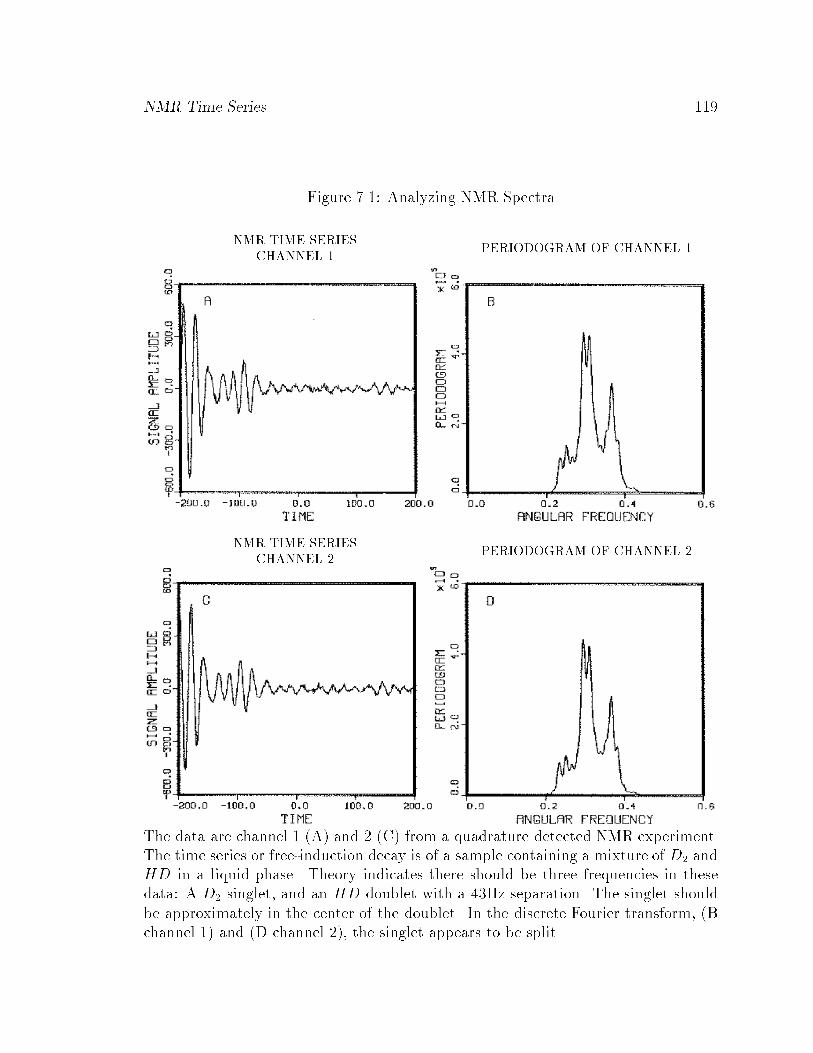
NMR Time Series 119
Figure 7.1: Analyzing NMR Spectra
NMR TIME SERIES
CHANNEL 1PERIODOGRAM OF CHANNEL 1
NMR TIME SERIES
CHANNEL 2PERIODOGRAM OF CHANNEL 2
The data are channel 1 (A) and 2 (C) from a quadrature detected NMR experiment.The time series or free-induction decay is of a sample containing a mixture of D2 andHD in a liquid phase. Theory indicates there should be three frequencies in thesedata: A D2 singlet, and an HD doublet with a 43Hz separation. The singlet shouldbe approximately in the center of the doublet. In the discrete Fourier transform, (Bchannel 1) and (D channel 2), the singlet appears to be split.

120 CHAPTER 7
Y �NXi=1
[d2(ti)� f2(ti)]2:
Because the amplitudes and noise variance are assumed di�erent in each channel, we
may remove these using the same procedure developed in Chapter 3.
As in most of our examples, this procedure is conservative; if we had de�nite prior
information linking the amplitude or variances in the two channels, we could exploit
that information at this point to get still better estimates of the f!g parameters.
For example, if we knew that the noise was strongly correlated in the two channels,
that would enable us to estimate the noise in each channel more accurately. After
removing the nuisance parameters, the marginal posterior probability of the f!gparameters is just the product of the \Student t-distributions" Eq. (3.17) for each
channel separately:
P (f!gjD; I) /"1� mh21
Nd21
#m�N2"1 � mh22
Nd22
#m�N2
(7:1)
where the subscripts refer to the channel number. As explained previously, (7.1) in
e�ect estimates the noise level independently in the two channels. This procedure is
general and can be applied whenever two measurements of a signal are available; it
is not restricted to NMR data. It is possible to specialize the estimation procedures
to include this quadrature model, as well as the aforementioned phase and noise
correlations. If all of this prior information is incorporated into the analysis (the
author has, in fact, done this), we would expect to improve the results considerably.
However, the present results will prove adequate for most purposes.
A procedure for dealing with the multiple frequency problem was outlined in Chap-
ter VI, and we will apply that procedure here. The �rst step in any frequency esti-
mation problem is to plot the data and the log of the probability of a single harmonic
frequency. If there is only one data channel, this is essentially the periodogram of the
data, Fig. 7.1(B) and Fig. 7.1(D). When more than one channel is present, the log
probability of a single harmonic frequency is essentially the sum of the periodograms
for each channel, weighted by the appropriate reciprocal variances. If the variances
are unknown, then the appropriate statistic is the log of (7.1), shown in Fig. 7.2.
Now as was shown in Chapter 6, if the frequencies are well separated, a peak in
the periodogram above the noise level is evidence { but not proof { of a frequency
near that peak. From examining Fig. 7.2 we see there are nine resolved peaks in
0:2 < ! < 0:4 and suggestions of �ve more unresolved ones. This is many more
peaks than theoretical physics indicates there should be. Is this evidence of more

NMR Time Series 121
Figure 7.2: The Log10 Probability of One Frequency in Both Channels
When more than one channel is present, the periodogram is not the proper statisticto be analyzed for indications of a simple harmonic frequency. The proper statistic(shown above) is log of the probability of a single harmonic frequency in both channels.

122 CHAPTER 7
going on than theory predicts? To answer this question we will apply the general
procedure outlined in the preceding chapter for determining multiple frequencies. We
�rst �t the data with the single best frequency plus decay. We choose Lorentzian
decay instead of Gaussian because physical theory indicates the decay is Lorentzian
in a liquid phase. The model we used is
f1(t) = [B1 cos(!1t) +B2 sin(!1t)]e��t:
The computer code in Appendix E was used to evaluate the \Student t-distribution"
Eq. (3.17) for each channel, and these were multiplied to obtain, Eq. (7.1). We
searched in the two dimensional parameter space until we located the maximumof the
distribution by the \pattern" searching procedure noted before. Next we computed
the signal having the predicted parameters. The model (dotted line) and the data
from the real channel are shown in, Fig. 7.3(A). It is clear from examining this �gure
as well as from examining the residuals in, Fig. 7.3(B), that there is at least a second
frequency in this data. We see from the probability of a single harmonic frequency in
the residuals, Fig. 7.3(C), that there is still strong evidence for additional frequencies
near 0.3.
We then proceeded to a two-frequency-plus-decay model and repeated this pro-
cedure. That is, we estimated the second frequency plus decay from the residuals,
and then used the results from the one-frequency model plus the estimates from the
residuals as the initial estimates in a two-frequency model of the original data. We
searched this four-parameter space until we located the maximum of the probability
density. The results from the two-frequency model are displayed in Fig. 7.4. The
model (dotted line) now takes on more characteristics of the signal (A), while the
residuals (B) and the probability of a single harmonic frequency in the residuals (C)
continue to show evidence for additional e�ects in the data. Notice the structure of
the probability of a single frequency in the residuals. The addition of a second fre-
quency removed one peak and essentially left the others unchanged. We demonstrated
in Chapter 6 that when the frequencies are well separated the multiple-frequency es-
timation problem separates into a series of single-frequency problems, and this just
con�rms numerically that result.
To compare the two-frequency model to the one-frequency we computed the pos-
terior odds ratio, this is given by:
posterior odds =P (f2jI)P (f1jI)
P (Djf2; I)P (Djf1; I)
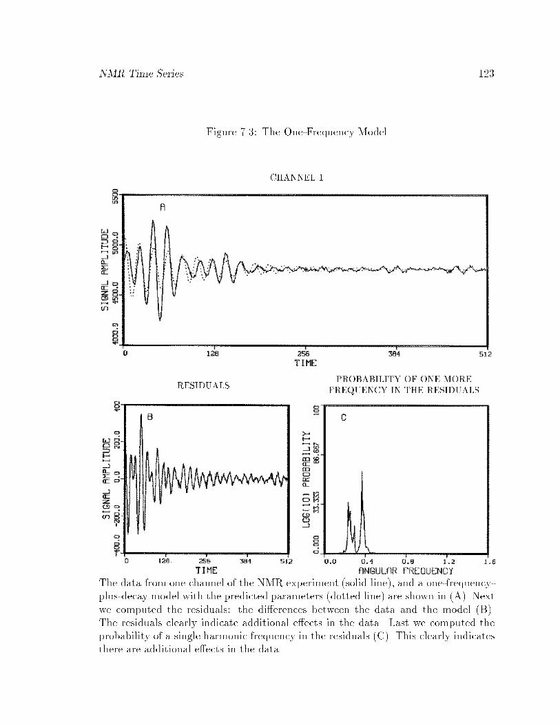
NMR Time Series 123
Figure 7.3: The One-Frequency Model
CHANNEL 1
RESIDUALSPROBABILITY OF ONE MORE
FREQUENCY IN THE RESIDUALS
The data from one channel of the NMR experiment (solid line), and a one-frequency-plus-decay model with the predicted parameters (dotted line) are shown in (A). Nextwe computed the residuals: the di�erences between the data and the model (B).The residuals clearly indicate additional e�ects in the data. Last we computed theprobability of a single harmonic frequency in the residuals (C). This clearly indicatesthere are additional e�ects in the data.
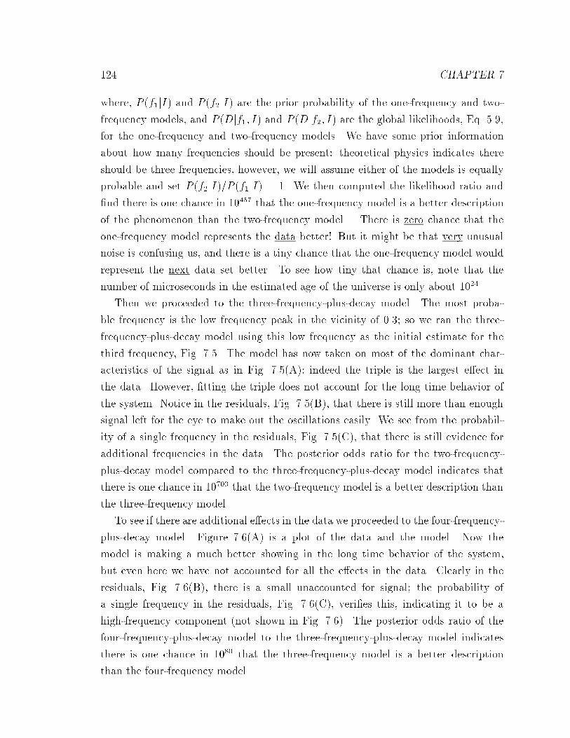
124 CHAPTER 7
where, P (f1jI) and P (f2jI) are the prior probability of the one-frequency and two-
frequency models, and P (Djf1; I) and P (Djf2; I) are the global likelihoods, Eq. 5.9,for the one-frequency and two-frequency models. We have some prior information
about how many frequencies should be present: theoretical physics indicates there
should be three frequencies, however, we will assume either of the models is equally
probable and set P (f2jI)=P (f1jI) = 1. We then computed the likelihood ratio and
�nd there is one chance in 10457 that the one-frequency model is a better description
of the phenomenon than the two-frequency model. There is zero chance that the
one-frequency model represents the data better! But it might be that very unusual
noise is confusing us, and there is a tiny chance that the one-frequency model would
represent the next data set better. To see how tiny that chance is, note that the
number of microseconds in the estimated age of the universe is only about 1024.
Then we proceeded to the three-frequency-plus-decay model. The most proba-
ble frequency is the low frequency peak in the vicinity of 0.3; so we ran the three-
frequency-plus-decay model using this low frequency as the initial estimate for the
third frequency, Fig. 7.5. The model has now taken on most of the dominant char-
acteristics of the signal as in Fig. 7.5(A): indeed the triple is the largest e�ect in
the data. However, �tting the triple does not account for the long time behavior of
the system. Notice in the residuals, Fig. 7.5(B), that there is still more than enough
signal left for the eye to make out the oscillations easily. We see from the probabil-
ity of a single frequency in the residuals, Fig. 7.5(C), that there is still evidence for
additional frequencies in the data. The posterior odds ratio for the two-frequency-
plus-decay model compared to the three-frequency-plus-decay model indicates that
there is one chance in 10703 that the two-frequency model is a better description than
the three-frequency model.
To see if there are additional e�ects in the data we proceeded to the four-frequency-
plus-decay model. Figure 7.6(A) is a plot of the data and the model. Now the
model is making a much better showing in the long time behavior of the system,
but even here we have not accounted for all the e�ects in the data. Clearly in the
residuals, Fig. 7.6(B), there is a small unaccounted for signal; the probability of
a single frequency in the residuals, Fig. 7.6(C), veri�es this, indicating it to be a
high-frequency component (not shown in Fig. 7.6). The posterior odds ratio of the
four-frequency-plus-decay model to the three-frequency-plus-decay model indicates
there is one chance in 1080 that the three-frequency model is a better description
than the four-frequency model.

NMR Time Series 125
Figure 7.4: The Two-Frequency Model
CHANNEL 1
RESIDUALSPROBABILITY OF ONE MORE
FREQUENCY IN THE RESIDUALS
Next we computed the probability of two frequencies plus decay in both channels.The model (dotted line) and the data (solid line) are displayed in (A). The residuals(B) clearly indicate additional e�ects in the data. We then computed the probabilityof a single frequency in the residuals and displayed that in panel (C).
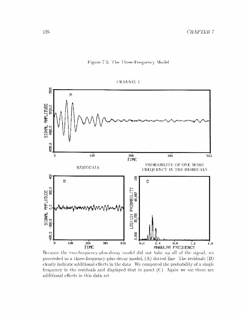
126 CHAPTER 7
Figure 7.5: The Three-Frequency Model
CHANNEL 1
RESIDUALSPROBABILITY OF ONE MORE
FREQUENCY IN THE RESIDUALS
Because the two-frequency-plus-decay model did not take up all of the signal, weproceeded to a three-frequency-plus-decay model, (A) dotted line. The residuals (B)clearly indicate additional e�ects in the data. We computed the probability of a singlefrequency in the residuals and displayed that in panel (C). Again we see there areadditional e�ects in this data set.
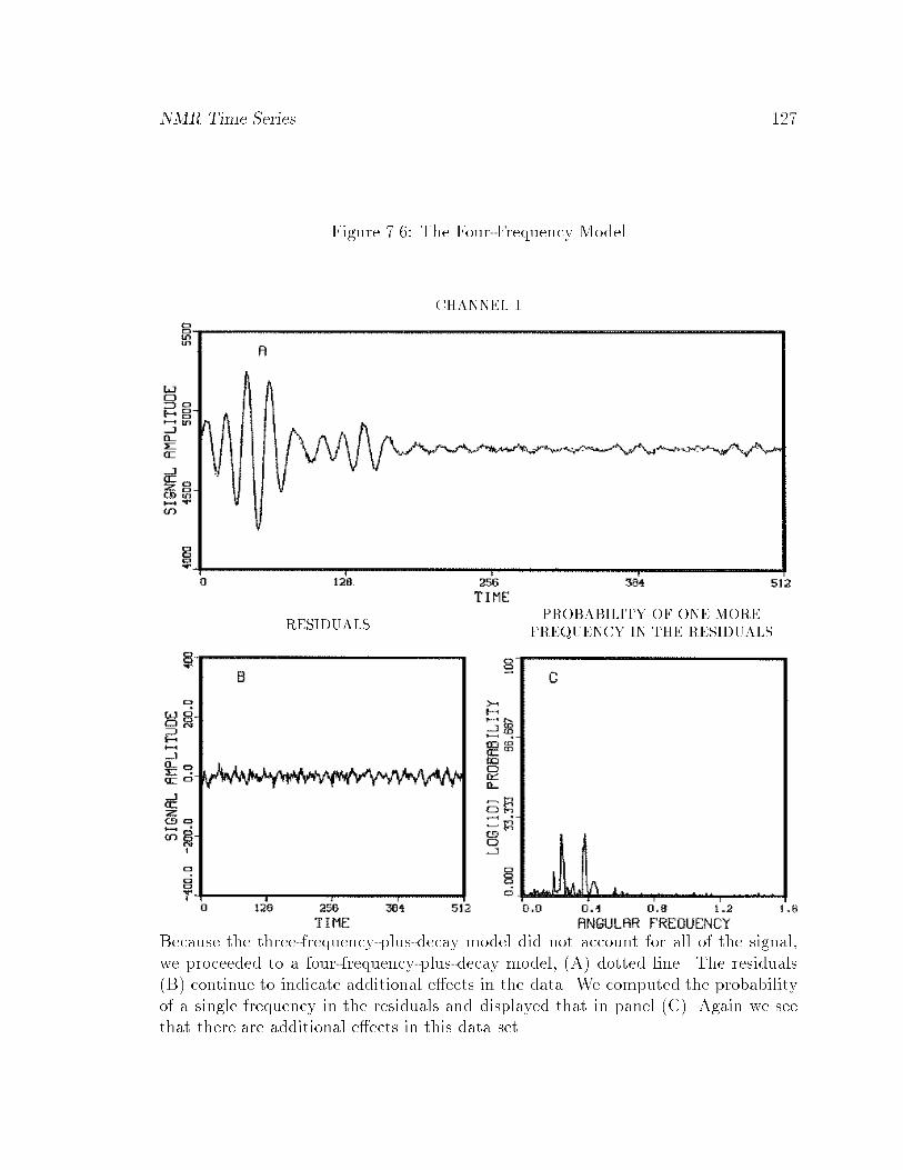
NMR Time Series 127
Figure 7.6: The Four-Frequency Model
CHANNEL 1
RESIDUALSPROBABILITY OF ONE MORE
FREQUENCY IN THE RESIDUALS
Because the three-frequency-plus-decay model did not account for all of the signal,we proceeded to a four-frequency-plus-decay model, (A) dotted line. The residuals(B) continue to indicate additional e�ects in the data. We computed the probabilityof a single frequency in the residuals and displayed that in panel (C). Again we seethat there are additional e�ects in this data set.

128 CHAPTER 7
We continued repeating this procedure until we accounted for all systematic com-
ponents { see Fig. 7.7 through Fig. 7.9. Now in Fig. 7.9(C) the residuals are �nally
beginning to look like Gaussian white noise. However, there is some evidence for
a very small additional frequency, see Fig. 7.9(C). We did not go further because
this frequency, although present in the real channel, is not present to any signi�cant
degree in the quadrature data channel.
Our probability analysis indicates there are at least seven frequencies in these data,
of which one is attributable to the instrumentation. That leaves six frequencies lo-
cated near 0.3 in dimensionless units. The posterior probability of a single harmonic
frequency in the combined data, Fig. 7.2, gives evidence of multiple complex phenom-
ena around 0.3 but it could not sort out what is going on. This is not too surprising,
given that there are six frequencies in this region. The one-frequency model has
done surprisingly well. The absorption spectrum, Fig. 7.10(A), on the other hand,
shows only three peaks in this region. This simple example illustrated that the dis-
crete Fourier transform gives evidence of frequencies in the data that an absorption
spectrum does not. Although the probability of a single harmonic frequency or the
Schuster periodogram is not an exact estimator for multiple frequencies, it is adequate
as long as the frequencies are well separated. The only time one must worry about
this statistic being incorrect is when the frequencies are close together (as they were
here). But by contrast, there are no conditions under which the absorption spectrum
is an optimal frequency estimator, and the global phase adjustment on the absorption
spectrum can suppress indications of frequencies in the data.
We developed the procedures for estimating the accuracy of the frequencies and
the amplitudes and we have used those procedures here [to apply them we calculated
the second derivatives numerically (4.13)]. The results of this calculation are:
Frequency Decay Rate Amplitude AmplitudeHertz Hertz Real Imaginary
75.0695 � 0.0005 7.294 � 0.003 49 4678.1231 � 0.0002 19.613 � 0.001 170 16094.1207 � 0.0008 8.569 � 0.001 71 7298.0187 � 0.0001 23.211 � 0.001 354 318117.6052 � 0.0001 16.336 � 0.001 193 188121.0824 � 0.0002 11.270 � 0.001 67 66
We also estimated the signal-to-noise ratio, Eq. (4.8), for each channel:
Signal
Noise= 1606 in channel 1,

NMR Time Series 129
Figure 7.7: The Five-Frequency Model
CHANNEL 1
RESIDUALSPROBABILITY OF ONE MORE
FREQUENCY IN THE RESIDUALS
Because the four-frequency model did not account for all of the signal, we proceededto a �ve-frequency model, (A) dotted line. The residuals (B) continue to indicateadditional e�ects in the data. We computed the probability of a single frequency inthe residuals and displayed that in panel (C). There is no apparent change in (C)because a very high frequency component was remove by the four-frequency model.Again we see that there are additional e�ects in this data set.
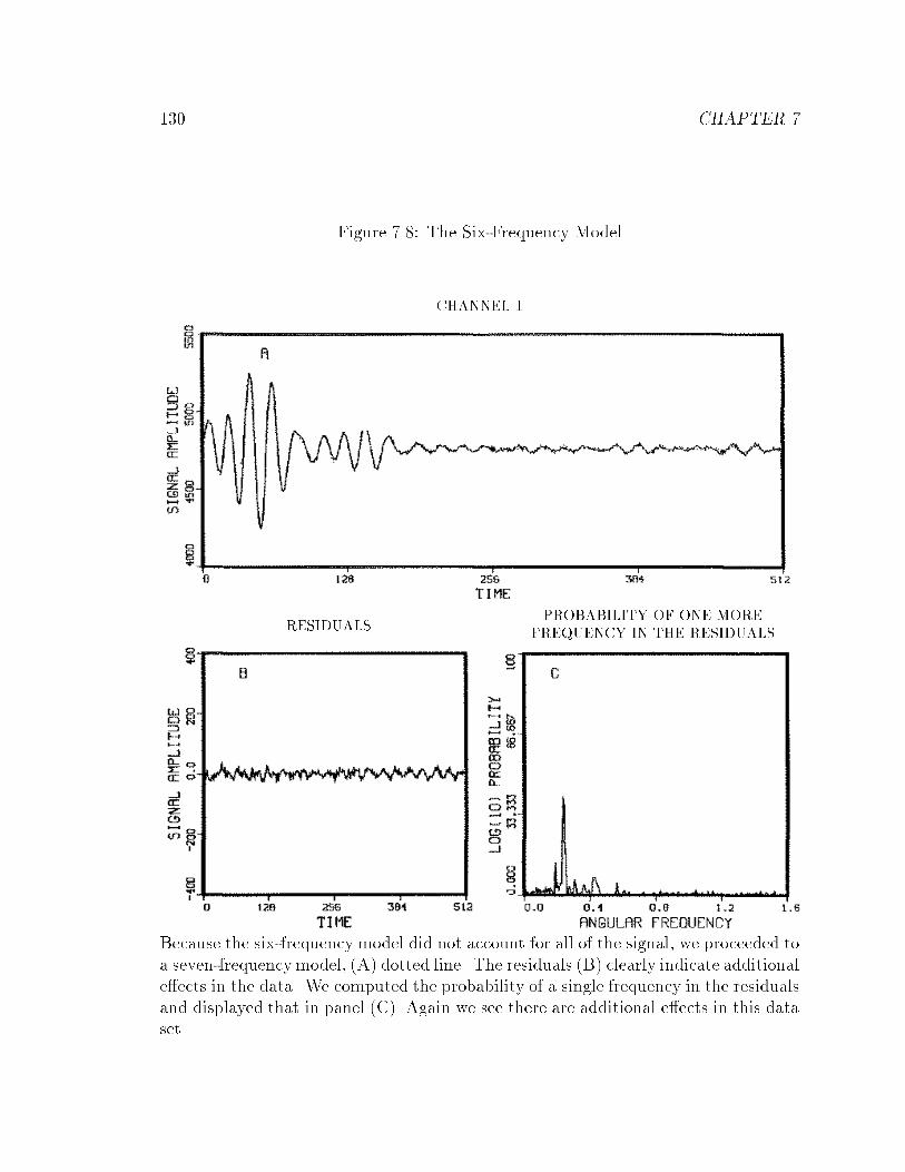
130 CHAPTER 7
Figure 7.8: The Six-Frequency Model
CHANNEL 1
RESIDUALSPROBABILITY OF ONE MORE
FREQUENCY IN THE RESIDUALS
Because the six-frequency model did not account for all of the signal, we proceeded toa seven-frequencymodel, (A) dotted line. The residuals (B) clearly indicate additionale�ects in the data. We computed the probability of a single frequency in the residualsand displayed that in panel (C). Again we see there are additional e�ects in this dataset.
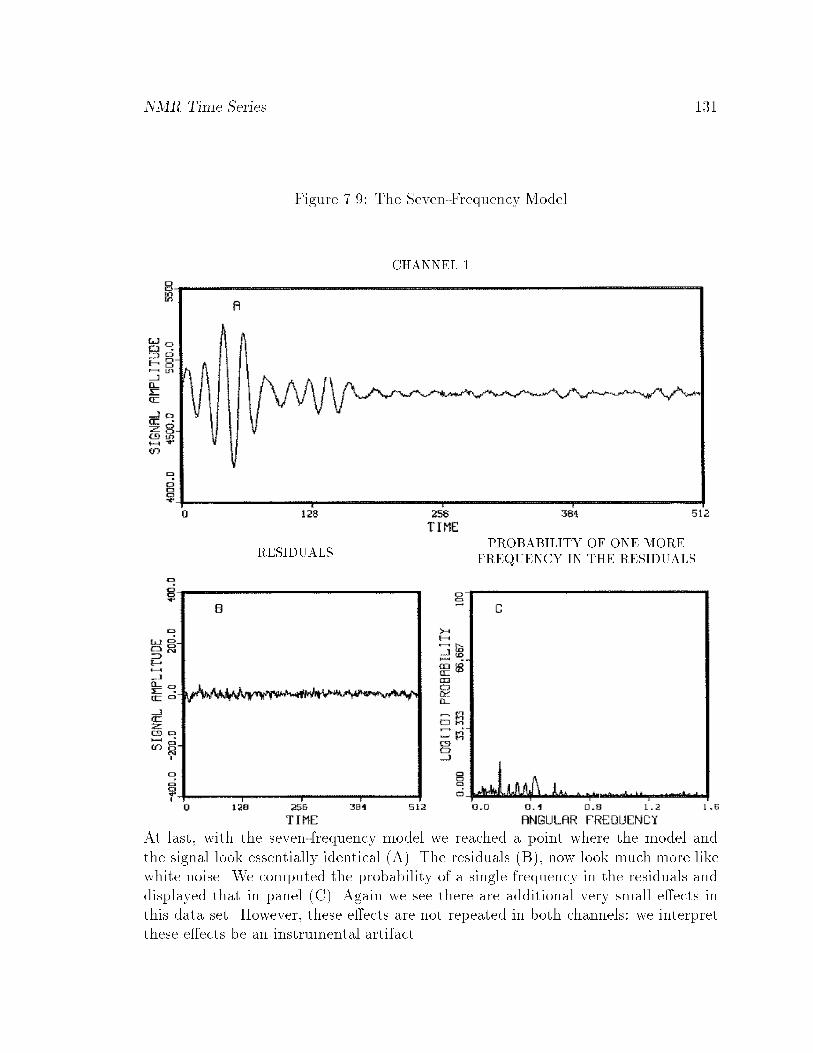
NMR Time Series 131
Figure 7.9: The Seven-Frequency Model
CHANNEL 1
RESIDUALSPROBABILITY OF ONE MORE
FREQUENCY IN THE RESIDUALS
At last, with the seven-frequency model we reached a point where the model andthe signal look essentially identical (A). The residuals (B), now look much more likewhite noise. We computed the probability of a single frequency in the residuals anddisplayed that in panel (C). Again we see there are additional very small e�ects inthis data set. However, these e�ects are not repeated in both channels: we interpretthese e�ects be an instrumental artifact.

132 CHAPTER 7
Figure 7.10: Comparison to an Absorption Spectrum
ABSORPTION SPECTRUM
POWER SPECTRAL DENSITY
The absorption spectrum (described in the text, see page 117) gives a clear indicationof three frequencies and hints at three others (A). Using the full width at half maxi-mum of the absorption spectrum to determine the accuracy estimate and convertingto physical units, it determines the frequencies to within �15Hz. The probabilityanalysis (B) used a seven-frequency model with decay. The estimated accuracy isapproximately �0:001Hz.
NMR Time Series 133
Signal
Noise= 1478 in channel 2,
and the estimated standard deviation (4.6):
(�)est = 9 in channel 1,
(�)est = 9 in channel 2.
The amplitudes were estimated separately in each channel, and if the spectrometer
is working correctly we expect the amplitude of each sinusoid to be approximately
the same. This serves as an additional check on the model; if we were �tting an
appreciable amount of noise, the estimated amplitudes would be di�erent in the two
channels.
The quantities of interest are the splitting between the two components of the HD
doublet as well as the shift in the center frequency. But physical theory indicated
there should be only three frequencies in the region of the main resonance: we �nd
six. The calculation indicates there is clearly more going on here than physical theory
indicates there should be. One of the major assumptions made in NMR is that the
magnetic �eld is uniform over the sample. If it is not, the resonances will be spread
out, corresponding to di�erent intensities of the local �eld, and false structure may
appear. Here we may be seeing this e�ect. However, the sharpness of the peaks
suggests that the e�ect is real, conceivably arising from impurities in the sample or
from association e�ects (such as H4O2 molecules) not considered in the theory.
However, we have derived a model of the process as if there were two major regions
in the sample where the �eld was approximately uniform. If we wish to derive the
splittings we must use the frequencies corresponding to uniform �eld. In each of
the regions where the �eld is a uniform, the frequency shifts should be according to
theory. Thus for the set of frequencies shifted to lower values (75, 94, and 117) the
HD doublet separation is
High - Low = 42:536 � 0:001Hz
and the center frequency (94 Hz) is displaced from the center of the doublet by
2.217�0.001 Hz. For the set of frequencies (78, 98, and 121) shifted to higher values
we have
High - Low = 42:956 � 0:001Hz
and the center frequency (98 Hz) is displaced from the center of the doublet by
1.521�0.001 Hz. Both of these tentative answers are in good agreement with the
134 CHAPTER 7
simple theory; unfortunately, until the �eld shimming problems are cleared up we
do not know which to believe, if either. The center frequency is displaced from the
center of the doublet in the correct direction, and in reasonable agreement with prior
measurements of this quantity [33]. In order to answer these questions it would be
necessary to rerun the experiment with better shimming. Additionally, the estimates
could be improved somewhat by sampling the data faster.
If one attempts to analyze these data using the standard absorption spectrum
Fig. 7.10(A) only three peaks are found, with hints of three other frequencies. The
splitting of the HD doublet is approximately correct, but the center peak is shifted
in the wrong direction. We can compare these estimates directly to the absorption
spectrum. The reason the analysis of this experiment is so di�cult with the absorp-
tion spectrum is that the full-width at half maximum for the D2 peak, Fig. 7.10(A),
is 15Hz. But this width is indicative only of the decay rates; not the accuracy with
which the oscillations frequency is determined. Probability theory has enabled us to
separate these entirely di�erent quantities. Figure 7.10(B) gives the estimates from
Eq. (7.1). We have plotted these estimates as normalized Gaussians, each centered
at the estimated frequency and having the same standard deviation as the estimated
frequency. Clearly, the resolution of these frequencies is much improved compared
to an absorption spectrum or a discrete Fourier transform. With separately normal-
ized distributions, the heights in Fig. 7.10(B) are indications of the accuracy of the
estimates, not of the power carried by the signal.
The accuracy of this procedure may be a little disturbing. To understand it, look
at the estimated signal-to-noise ratio in these data. It is on the order of 1500 for
each channel. There is essentially nothing in these data sets that can be ignored.
Every little bump and wiggle in the discrete Fourier transform is indicative of some
e�ect in the data, and must be accounted for. Because the accuracy of the estimates is
inversely proportional to the signal-to-noise of the data, the estimates are very precise.
It is rather the inaccuracy of the conventional method that should be disturbing to
one.
7.2 Corn Crop Yields
Economic data are hard to analyze, in part because the data are frequently con-
taminated by large spurious e�ects, which one does not know how to capture in a

Corn Crop Yields 135
model, and the time series are often very short. Here we will examine one example
of economic data to demonstrate how to remove some unknown and spurious e�ects.
In particular, we will analyze one hundred year's worth of corn crop data from three
states (Kansas, South Dakota, and Nebraska), Fig. 7.11(A) through Fig. 7.11(C) [34].
We would like to know if there is any indication of periodic behavior in these data.
These data have been analyzed before. Currie [35] used a high pass �lter and then
applied the Burg algorithm [36] to the �ltered data. Currie �nds one frequency near
20 years which is attributed to the lunar 18.6 year cycle, and another at 11 years,
which is attributed to the solar cycle.
There are three steps in Currie's analysis that are troublesome. First, the Burg
algorithm is not optimal in the presence of noise (although it is for the problem it was
formulated to solve). The fact that it continues to work means that the procedure
is reasonably robust; that does not change the fact that it is fundamentally not
appropriate to this problem [36]. Second, one has doubts about the �lter: could it
suppress the e�ect one is looking for or introduce other spurious e�ects? Third, to
apply the Burg algorithm when the data consist of the actual values of a time series,
the autoregression order (maximum lag to be used) must be chosen and there is no
theoretical principle to determine this choice. We do not mean to imply that Currie's
result is incorrect; only that it is provisional. We would like to apply probability
theory as developed in this work to check these results.
The �rst step in a harmonic analysis is simply to plot the data, Fig. 7.11(A)
through Fig. 7.11(C) and the log of the posterior probability of a single harmonic
frequency. In the previous example we generalized the analysis for two channels. The
generalization to an arbitrary number of channels is just a repeat of the previous
arguments:
P (f!gjD; I) /rY
j=1
"1 � mjh2j
Njd2j
#mj�Nj2
(7:2)
where the subscripts refer to the jth channels: each of the models has mj amplitudes,
and each data set contains Nj data values. Additionally it was assumed that the
noise variance �j was unknown and possibly di�erent for each channel. The \Stu-
dent t-distributions" Eq. (3.17) for each channel should be computed separately, thus
estimating and eliminating the nuisance parameters particular to that channel, and
then multiplied to obtain the posterior probability for the common e�ects, Eq. (7.2).
Again if we had prior knowledge of correlations in the \noise" for di�erent chan-
nels, we could exploit that information to get better �nal results, at the cost of more
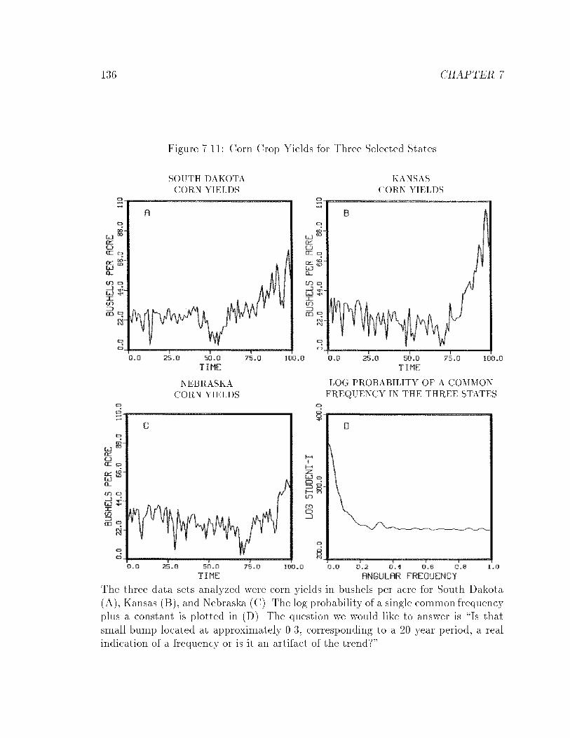
136 CHAPTER 7
Figure 7.11: Corn Crop Yields for Three Selected States
SOUTH DAKOTA
CORN YIELDS
KANSAS
CORN YIELDS
NEBRASKA
CORN YIELDS
LOG PROBABILITY OF A COMMON
FREQUENCY IN THE THREE STATES
The three data sets analyzed were corn yields in bushels per acre for South Dakota(A), Kansas (B), and Nebraska (C). The log probability of a single common frequencyplus a constant is plotted in (D). The question we would like to answer is \Is thatsmall bump located at approximately 0.3, corresponding to a 20 year period, a realindication of a frequency or is it an artifact of the trend?"

Corn Crop Yields 137
computation.
For this harmonic analysis we take the model to be a single sinusoid which oscillates
about a constant. The model for the jth channel may be written
fj(t) = Bj;1 +Bj;2 sin(!t) +Bj;3 cos(!t): (7:3)
Here we have three channels, named \South Dakota", \Kansas", and \Nebraska".
We allow Bj;1, Bj;2, and Bj;3 to be di�erent for each channel; thus there are a total of
nine amplitudes, one frequency, and three noise variances. To compute the posterior
probability for each measurement, we used the computer code in Appendix E. The
log of each \Student t-distribution" Eq. (3.17) was computed and added to obtain the
log of the posterior probability of a single common harmonic frequency, Fig. 7.11(D).
What we would like to know is, \Are those small bumps in Fig. 7.11(D) indications
of periodic behavior, or are they artifacts of the noise or trend?" To attempt to answer
this, consider the following model function
fj(t) = Tj(t) +Bj;1 cos(!t) +Bj;2 sin(!t)
where we have augmented the standard frequency model by a trend Tj(t). The only
parameter of interest is the frequency !. The trend Tj(t) is a nuisance function; to
eliminate it we expand the trend in orthonormal polynomials Lj(t). These orthonor-
mal polynomials could be any complete set. We use the Legendre polynomials with
an appropriate scaling of the independent variable to make them orthonormal on the
region (�49:5 � t � 49:5). This is the range of values used for the time index in
the sine and cosine terms. After expanding the trend, the model function for the jth
measurement can be written
fj(t) =EXk=0
Bj;k+1Lk(t) +Bj;E+2 cos(!t) +Bj;E+3 sin(!t):
Notice that if the expansion order E is zero the problem is reduced to the previous
problem (7.3).
The expansion order E must be set to some appropriate value. From looking at
these data one sees that it will take at least a second order expansion to remove the
trend. The actual expansion order for the trend is unknown. However, it will turn
out that the estimated frequencies are insensitive to the expansion order, as long as
the expansion is su�cient to represent the trend without representing the signal of
interest. Of course, di�erent orders could have very di�erent implications about other
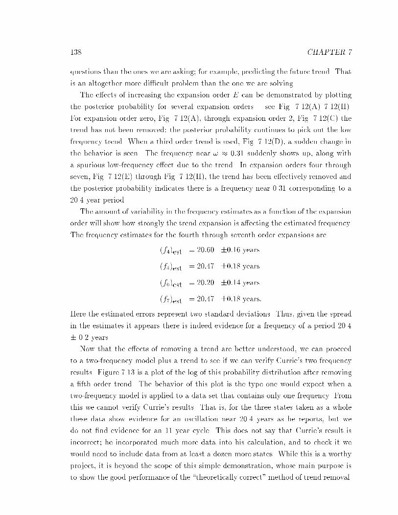
138 CHAPTER 7
questions than the ones we are asking; for example, predicting the future trend. That
is an altogether more di�cult problem than the one we are solving.
The e�ects of increasing the expansion order E can be demonstrated by plotting
the posterior probability for several expansion orders { see Fig. 7.12(A){7.12(H).
For expansion order zero, Fig. 7.12(A), through expansion order 2, Fig. 7.12(C) the
trend has not been removed: the posterior probability continues to pick out the low
frequency trend. When a third order trend is used, Fig. 7.12(D), a sudden change in
the behavior is seen. The frequency near ! � 0:31 suddenly shows up, along with
a spurious low-frequency e�ect due to the trend. In expansion orders four through
seven, Fig. 7.12(E) through Fig. 7.12(H), the trend has been e�ectively removed and
the posterior probability indicates there is a frequency near 0.31 corresponding to a
20.4 year period.
The amount of variability in the frequency estimates as a function of the expansion
order will show how strongly the trend expansion is a�ecting the estimated frequency.
The frequency estimates for the fourth through seventh order expansions are
(f4)est = 20:60 �0:16 years
(f5)est = 20:47 �0:18 years
(f6)est = 20:20 �0:14 years
(f7)est = 20:47 �0:18 years:
Here the estimated errors represent two standard deviations. Thus, given the spread
in the estimates it appears there is indeed evidence for a frequency of a period 20.4
� 0.2 years.
Now that the e�ects of removing a trend are better understood, we can proceed
to a two-frequency model plus a trend to see if we can verify Currie's two frequency
results. Figure 7.13 is a plot of the log of this probability distribution after removing
a �fth order trend. The behavior of this plot is the type one would expect when a
two-frequency model is applied to a data set that contains only one frequency. From
this we cannot verify Currie's results. That is, for the three states taken as a whole
these data show evidence for an oscillation near 20.4 years as he reports, but we
do not �nd evidence for an 11 year cycle. This does not say that Currie's result is
incorrect; he incorporated much more data into his calculation, and to check it we
would need to include data from at least a dozen more states. While this is a worthy
project, it is beyond the scope of this simple demonstration, whose main purpose is
to show the good performance of the \theoretically correct" method of trend removal.

Corn Crop Yields 139
Figure 7.12: The Joint Probability of a Frequency Plus a Trend
PROBABILITY OF A HARMONIC FREQUENCY
IN THE CORN YIELD DATA WITH
A CONSTANT CORRECTION
PROBABILITY OF A HARMONIC FREQUENCY
IN THE CORN YIELD DATA WITH
A FIRST ORDER TREND CORRECTION
By including a trend expansion in our model we e�ectively look for oscillations abouta trend. This is not the same as detrending, because the trend functions and the sineand cosine functions are never orthogonal. The zero order trend (or constant) plus asimple-harmonic-frequency model (A) is dominated by the trend. When we includeda linear trend the height of the trend is decreased some, however the trend is still thedominant e�ect in the analysis.

140 CHAPTER 7
PROBABILITY OF A HARMONIC FREQUENCY
IN THE CORN YIELD DATA WITH
A SECOND ORDER TREND CORRECTION
PROBABILITY OF A HARMONIC FREQUENCY
IN THE CORN YIELD DATA WITH
A THIRD ORDER TREND CORRECTION
The probability of a single harmonic frequency plus a second-order trend (C) continuesto pick out the low frequency trend. However, the level and spread of the marginalposterior probability density is such that the trend has almost been removed. Whenthe probability of a single harmonic frequency plus a third-order trend is computed,the probability density suddenly changes behavior. The frequency near 0.3 is now thedominant feature (D). The trend has not been completely removed; a small artifactpersists at low frequencies.
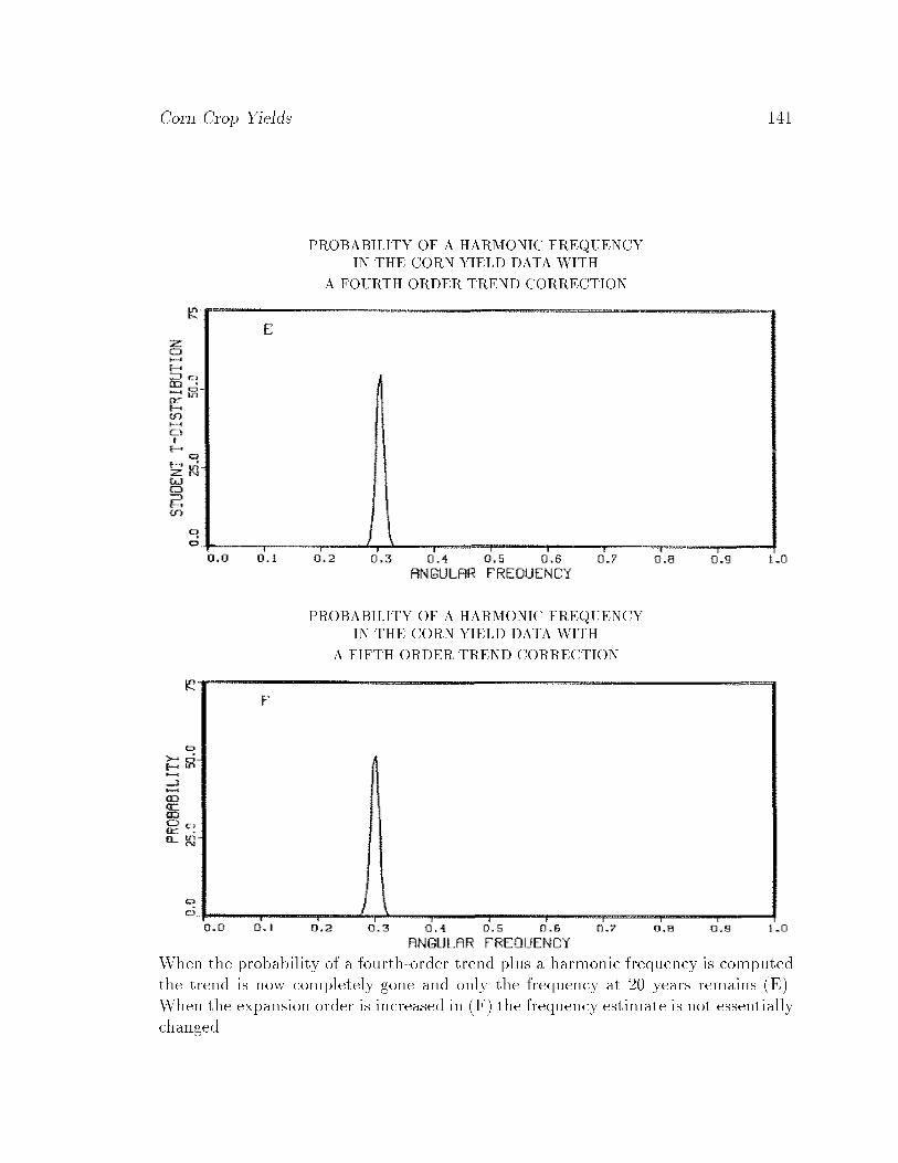
Corn Crop Yields 141
PROBABILITY OF A HARMONIC FREQUENCY
IN THE CORN YIELD DATA WITH
A FOURTH ORDER TREND CORRECTION
PROBABILITY OF A HARMONIC FREQUENCY
IN THE CORN YIELD DATA WITH
A FIFTH ORDER TREND CORRECTION
When the probability of a fourth-order trend plus a harmonic frequency is computedthe trend is now completely gone and only the frequency at 20 years remains (E).When the expansion order is increased in (F) the frequency estimate is not essentiallychanged.
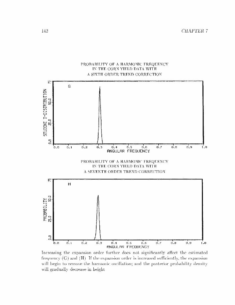
142 CHAPTER 7
PROBABILITY OF A HARMONIC FREQUENCY
IN THE CORN YIELD DATA WITH
A SIXTH ORDER TREND CORRECTION
PROBABILITY OF A HARMONIC FREQUENCY
IN THE CORN YIELD DATA WITH
A SEVENTH ORDER TREND CORRECTION
Increasing the expansion order further does not signi�cantly a�ect the estimatedfrequency (G) and (H). If the expansion order is increased su�ciently, the expansionwill begin to remove the harmonic oscillation; and the posterior probability densitywill gradually decrease in height.
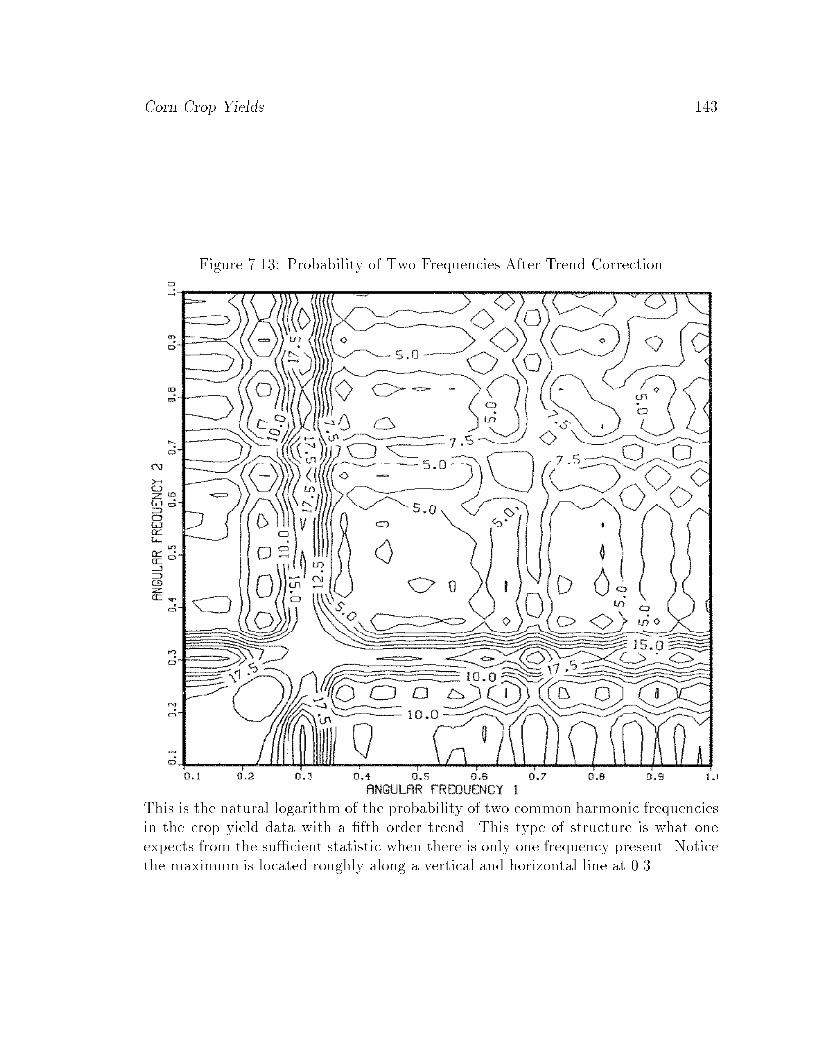
Corn Crop Yields 143
Figure 7.13: Probability of Two Frequencies After Trend Correction
This is the natural logarithm of the probability of two common harmonic frequenciesin the crop yield data with a �fth order trend. This type of structure is what oneexpects from the su�cient statistic when there is only one frequency present. Noticethe maximum is located roughly along a vertical and horizontal line at 0.3.
144 CHAPTER 7
We did not seek to remove the trend from the data, but rather to eliminate its e�ect
from the conclusions.
7.3 Another NMR Example
Now that the tools have been developed we can demonstrate how one can incor-
porate partial information about a model. In the corn crop example the trend was
unknown, so it was expanded in orthonormal polynomials and integrated out of the
problem, while we included what partial information we had in the form of the sine
and cosine terms. In this NMR example let us assume that the decay function is of
interest to us. We would like to determine this function as accurately as possible.
The data we used, Fig. 7.14(A), in this example are one channel of a pure D2
spectrum [31]. Figure 7.14(B) contains the periodogram for these data. For this
demonstration we will use the �rst N = 512 data points because they contain most
of the signal.
For D2, theoretical studies indicate there is a single frequency with decay [32].
Now we expect the signal should have the form
f(t) = [B1 sin(!t) +B2 cos(!t)]D(t);
where D(t) is the decay function, and the sine and cosine e�ectively express what
partial information we have about the signal. We will expand the decay function D(t)
to obtain
f(t) = [B1 sin(!t) +B2 cos(!t)]rX
j=0
DjLj(t)
where Dj are the expansion coe�cients for the decay function, B1 and B2 are e�ec-
tively the amplitude and phase of the sinusoidal oscillations, and Lj are the Legendre
polynomials with the appropriate change of variables. This model can be rewritten
as
f(t) =rX
j=0
DjB1
�Lj(t)[sin(!t) +
B2
B1
cos(!t)]�:
There is an indeterminacy in the overall scale. That is, the amplitude of the
sinusoid and the amplitude of the decay D(t) cannot both be determined. One of
them is necessarily arbitrary. We chose the amplitude of the sine term to be unity
because it e�ectively eliminates one f!g parameter from the problem. We have a
choice, in this problem, on which parameters are to be removed by integration. We
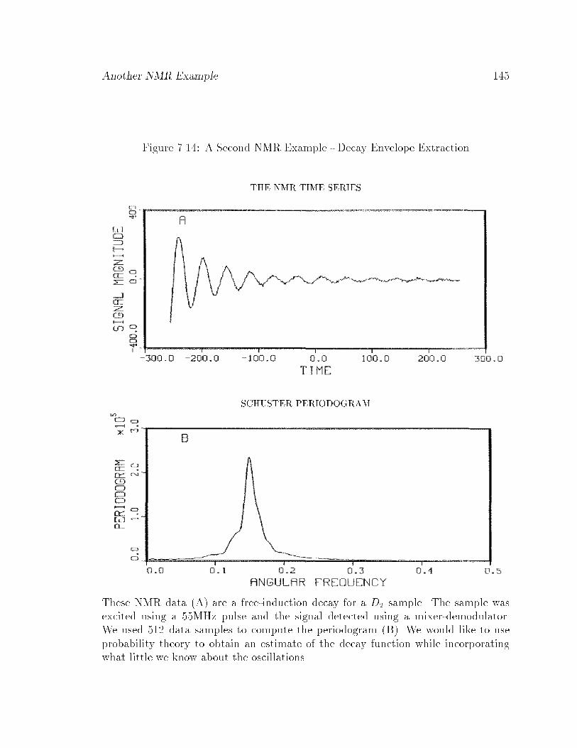
Another NMR Example 145
Figure 7.14: A Second NMR Example - Decay Envelope Extraction
THE NMR TIME SERIES
SCHUSTER PERIODOGRAM
These NMR data (A) are a free-induction decay for a D2 sample. The sample wasexcited using a 55MHz pulse and the signal detected using a mixer-demodulator.We used 512 data samples to compute the periodogram (B). We would like to useprobability theory to obtain an estimate of the decay function while incorporatingwhat little we know about the oscillations.
146 CHAPTER 7
chose to eliminate fDjB1g because there are many more of them, even though they
are really the parameters of interest.
When we eliminate a parameter from the problem, it does not mean that it cannot
be estimated. In fact, we can always calculate the parameters fDjB1g from the linear
relations between models, Eq. (4.2). For this problem it is simpler to search for the
maximum of the probability distribution as a function of frequency ! and the ratio
B1=B2, and then use Eq. (4.2) to compute the expansion coe�cientsDj . If we choose
to eliminate the amplitudes of the sine and cosine terms, then we must search for the
maximum of the probability distribution as a function of the expansion parameters;
there could be a large number of these.
We must again set the expansion order r; here we have plenty of data so in principle
we could take r to be large. However, unless the decay is rapidly varying we would
expect a moderate expansion of perhaps 5th to 10th order to be more than adequate.
In the examples given here we set the expansion order to 10. We solved the problem
also with the expansion order set to 5, and the results were e�ectively identical to the
tenth order expansion.
To solve this problem we again used the computer code in Appendix E, and the
\pattern" search routine discussed earlier. We located the maximum of the two
dimensional \Student t-distribution," Eq. (3.17), and used the procedure given in
Chapter 4, Eqs. (4.9) through (4.14), to estimate the standard deviation of the pa-
rameters. We �nd these to be
(!)est = 0:14976 � 2 � 10�5
�B2
B1
�est
= �:475 � 5� 10�3
at two standard deviations. The variance of these data was d2 = 2902, the estimated
noise variance (�2)est � 27:1, and the signal-to-noise ratio was 23.3.
After locating the maximum of the probability density we used the linear rela-
tions (4.2) between the orthonormal model and the nonorthonormal model to com-
pute the expansion coe�cients. We set the scale by requiring the decay function and
the reconstructed model function to touch at one point near the global maximum. We
have plotted the data and the estimated decay function, Fig. 7.15(A). In Fig. 7.15(B)
we have a close up of the data, the decay function, and the reconstructed signal.
It is apparent from this plot that the decay is not Lorentzian or there is a second
very small frequency present in the data. The decay function drops rapidly and then
begins to oscillate. This is a real e�ect and is not an artifact of the procedure we are
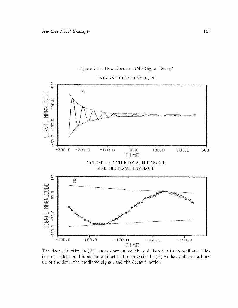
Another NMR Example 147
Figure 7.15: How Does an NMR Signal Decay?
DATA AND DECAY ENVELOPE
A CLOSE UP OF THE DATA, THE MODEL,
AND THE DECAY ENVELOPE
The decay function in (A) comes down smoothly and then begins to oscillate. Thisis a real e�ect, and is not an artifact of the analysis. In (B) we have plotted a blowup of the data, the predicted signal, and the decay function.
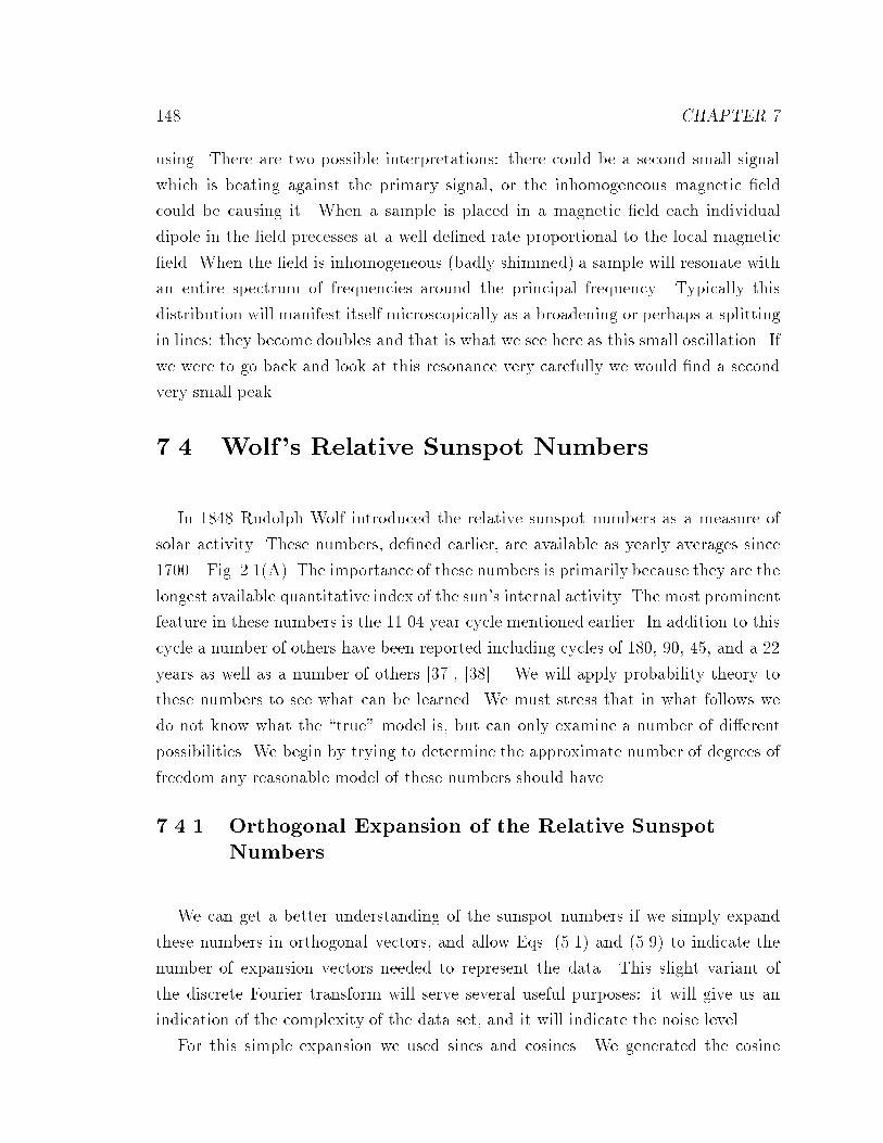
148 CHAPTER 7
using. There are two possible interpretations: there could be a second small signal
which is beating against the primary signal, or the inhomogeneous magnetic �eld
could be causing it. When a sample is placed in a magnetic �eld each individual
dipole in the �eld precesses at a well de�ned rate proportional to the local magnetic
�eld. When the �eld is inhomogeneous (badly shimmed) a sample will resonate with
an entire spectrum of frequencies around the principal frequency. Typically this
distribution will manifest itself microscopically as a broadening or perhaps a splitting
in lines: they become doubles and that is what we see here as this small oscillation. If
we were to go back and look at this resonance very carefully we would �nd a second
very small peak.
7.4 Wolf's Relative Sunspot Numbers
In 1848 Rudolph Wolf introduced the relative sunspot numbers as a measure of
solar activity. These numbers, de�ned earlier, are available as yearly averages since
1700 { Fig. 2.1(A). The importance of these numbers is primarily because they are the
longest available quantitative index of the sun's internal activity. The most prominent
feature in these numbers is the 11.04 year cycle mentioned earlier. In addition to this
cycle a number of others have been reported including cycles of 180, 90, 45, and a 22
years as well as a number of others [37], [38]. We will apply probability theory to
these numbers to see what can be learned. We must stress that in what follows we
do not know what the \true" model is, but can only examine a number of di�erent
possibilities. We begin by trying to determine the approximate number of degrees of
freedom any reasonable model of these numbers should have.
7.4.1 Orthogonal Expansion of the Relative Sunspot
Numbers
We can get a better understanding of the sunspot numbers if we simply expand
these numbers in orthogonal vectors, and allow Eqs. (5.1) and (5.9) to indicate the
number of expansion vectors needed to represent the data. This slight variant of
the discrete Fourier transform will serve several useful purposes: it will give us an
indication of the complexity of the data set, and it will indicate the noise level.
For this simple expansion we used sines and cosines. We generated the cosine

Orthogonal Expansion of the Relative Sunspot Numbers 149
vectors using
Hj(ti) =1pcjcos
��jti
N
�
cj �NXi=1
cos2��jti
N
�
and the sine vectors using
Hk(ti) =1psj
sin
�kti
N
!
sj �NXi=1
sin2 �kti
N
!
where 0 � k � N=2 for the cosine components and 1 � k � N=2 for the sine
components. There are a total of 285 expansion vectors, and for this problem the
time increments are one year. Next we computed hk: the dot product between the
data and the expansion vectors. Both the sine and cosine dot products were then
squared and sorted into decreasing order.
From these ordered projections we could then easily compute the probability of
the expansion order E. For this problem this is essentially the posterior probability
Eq. (5.9) with r = 0 and the terms associated with the f!g set equal to 1. Because weare using an orthonormal expansion the Jacobian is unity. This simpli�es Eq. (5.9)
somewhat; we have
P (EjD; I) = ��E
2
���N �E
2
�"E(h2)E
2
#�E2 �N � E
2h�2i
�E�N2
;
where (h2)E is the su�cient statistic computed with the E largest orthonormal pro-
jections. Figure 7.16 is a plot of the posterior probability of the model as a function
of expansion order E. One can see from the plot that there is a peak in the proba-
bility around 90, and if one wants to be certain that all of the systematic component
has been expanded, then the expansion order must be taken to be approximately
100. The estimated signal-to-noise ratio of these data is approximately 11.5, and the
estimated standard deviation is about 5.
An orthogonal expansion of the data is about the worst model one could pick, in
the sense of having the largest number of degrees of freedom. If we were to produce
a model that reduced the total number of degrees of freedom by a factor 3 we would
still have over thirty. For a simple harmonic frequency model, that would be 10 to
14 total frequencies. There are 286 data values, and the main period of roughly 11
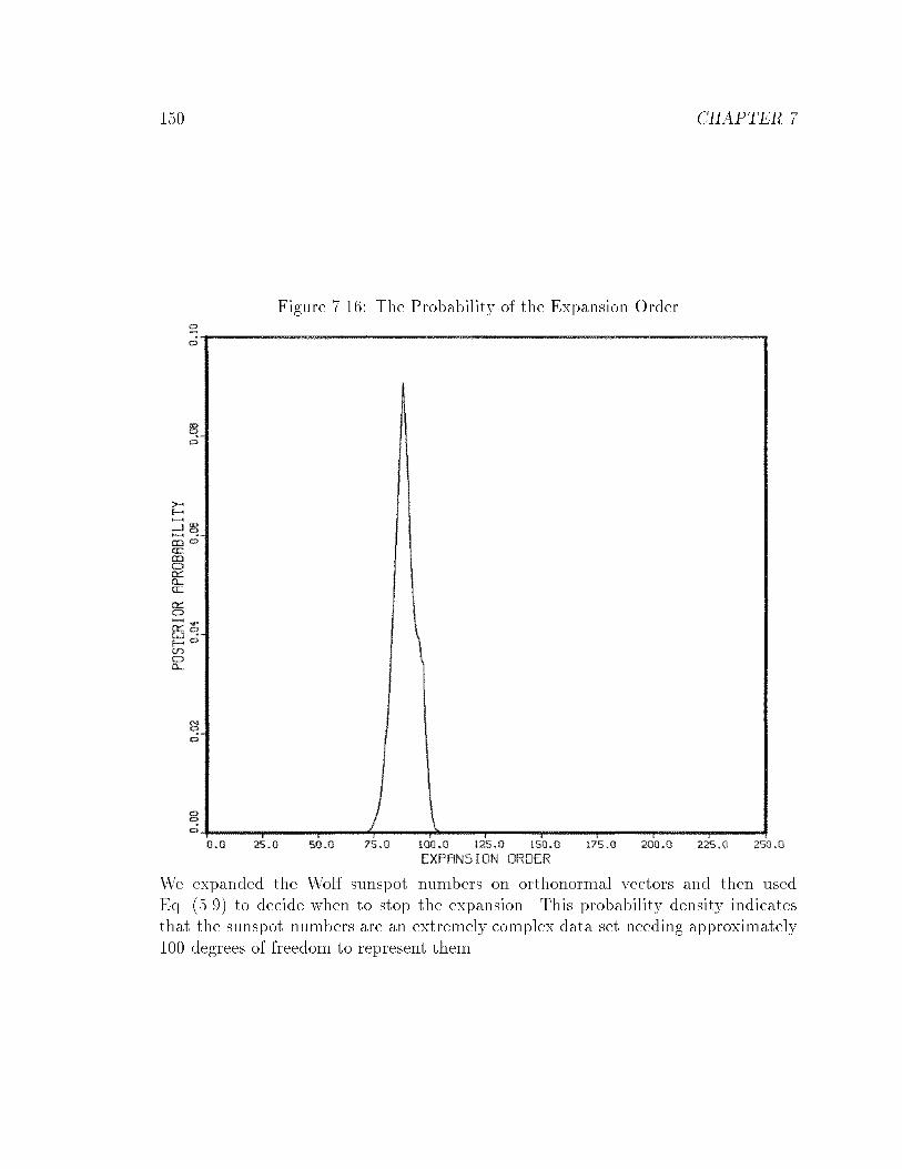
150 CHAPTER 7
Figure 7.16: The Probability of the Expansion Order
We expanded the Wolf sunspot numbers on orthonormal vectors and then usedEq. (5.9) to decide when to stop the expansion. This probability density indicatesthat the sunspot numbers are an extremely complex data set needing approximately100 degrees of freedom to represent them.
Harmonic Analysis of the Relative Sunspot Numbers 151
years; that gives 26 cycles in the record. If each period has a unique amplitude, that
still leaves approximately six to ten degrees of freedom to describe the shape of the
oscillation. The implication of this is that Wolf's numbers are intrinsically extremely
complicated, and no simple model for these numbers is going to prove possible. We
will investigate them using a number of relatively simple models to see what can be
learned.
7.4.2 Harmonic Analysis of the
Relative Sunspot Numbers
The second model we will investigate is the multiple harmonic frequency model.
There are three degrees of freedom for each frequency, and with 100 degrees of freedom
in the data, there is no chance of �nding all of the structure in them. We will content
ourselves with �nding the �rst few frequencies and seeing how the results compare
with the orthogonal expansion. Many writers have performed a harmonic analysis
on these numbers. We will compare our results to those obtained recently by Sonett
[38] and Bracewell [39]. The analysis done by Sonett concentrated on determining
the spectrum of the relative sunspot numbers. He used the Burg [36] algorithm.
This routine is extremely sensitive to the frequencies. In addition to �nding the
frequencies, this routine will sometimes shift the location of the predicted frequency,
and it estimates a spectral density (a power normalized probability distribution), not
the power carried in a line. Consequently, no accurate determination of the power
carried by these lines has been done. As explained by Jaynes [40], the Burg algorithm
yields the optimal solution to a certain well-de�ned problem. But in practice it is used
in some very di�erent problems for which it is not optimal (although still useful). We
will use probability theory to estimate the frequencies, their accuracy, the amplitudes,
the phases, as well as the power carried by each line.
Again, we plot the log of the probability of a single harmonic frequency plus a
constant, Fig. 7.17(A). In this study, we include a constant and allow probability
theory to remove it the correct way, instead of subtracting the average from the data
as was done in Chapter 2. We do this to see if this theoretically correct way of
eliminating a constant will make any di�erence in the evidence for frequencies. Thus
we plot the log of the marginal posterior probability Eq. (3.17) using
f(t) = B1 +B2 cos!t+B3 sin!t
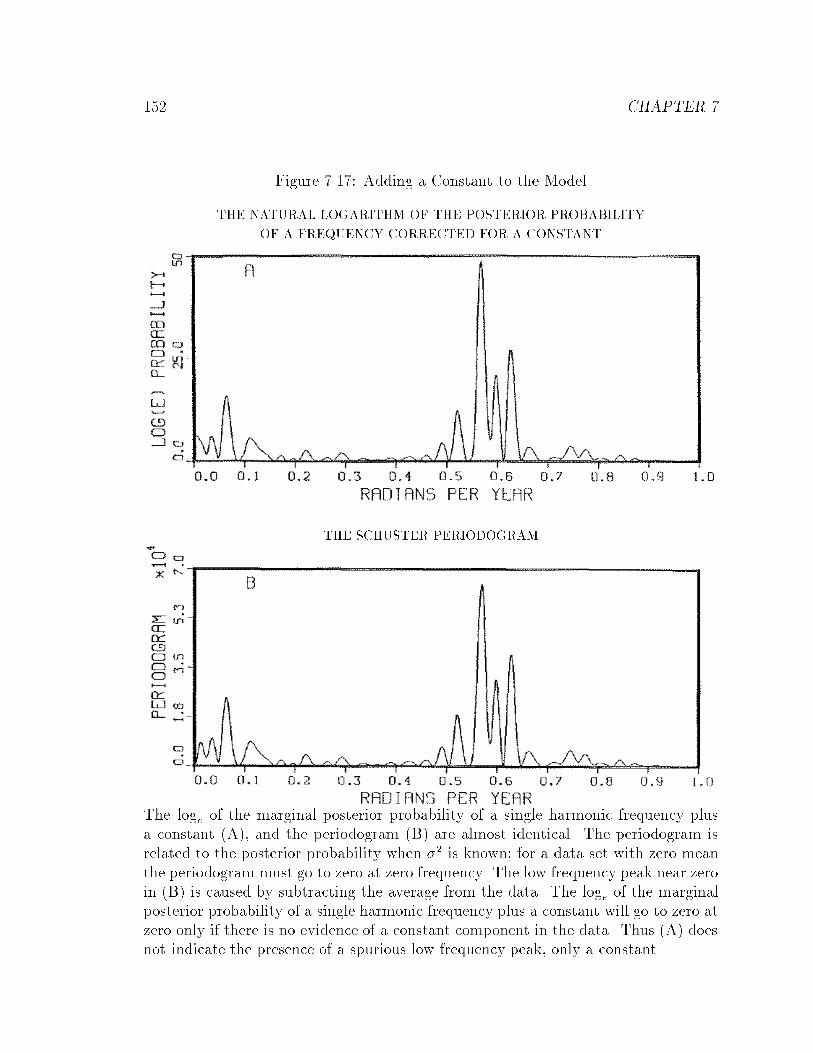
152 CHAPTER 7
Figure 7.17: Adding a Constant to the Model
THE NATURAL LOGARITHM OF THE POSTERIOR PROBABILITY
OF A FREQUENCY CORRECTED FOR A CONSTANT
THE SCHUSTER PERIODOGRAM
The loge of the marginal posterior probability of a single harmonic frequency plusa constant (A), and the periodogram (B) are almost identical. The periodogram isrelated to the posterior probability when �2 is known; for a data set with zero meanthe periodogram must go to zero at zero frequency. The low frequency peak near zeroin (B) is caused by subtracting the average from the data. The loge of the marginalposterior probability of a single harmonic frequency plus a constant will go to zero atzero only if there is no evidence of a constant component in the data. Thus (A) doesnot indicate the presence of a spurious low frequency peak, only a constant.
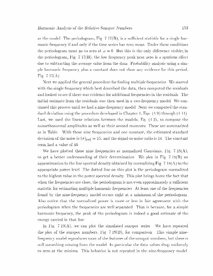
Harmonic Analysis of the Relative Sunspot Numbers 153
as the model. The periodogram, Fig. 7.17(B), is a su�cient statistic for a single har-
monic frequency if and only if the time series has zero mean. Under these conditions
the periodogram must go to zero at ! = 0. But this is the only di�erence visible; in
the periodogram, Fig. 7.17(B), the low frequency peak near zero is a spurious e�ect
due to subtracting the average value from the data. Probability analysis using a sim-
ple harmonic frequency plus a constant does not show any evidence for this period,
Fig. 7.17(A).
Next we applied the general procedure for �nding multiple frequencies. We started
with the single frequency which best described the data, then computed the residuals
and looked to see if there was evidence for additional frequencies in the residuals. The
initial estimate from the residuals was then used in a two-frequency model. We con-
tinued this process until we had a nine-frequency model. Next we computed the stan-
dard deviation using the procedure developed in Chapter 4, Eqs. (4.9) through (4.14).
Last, we used the linear relations between the models, Eq. (4.2), to compute the
nonorthonormal amplitudes as well as their second moments. These are summarized
as in Table . With these nine frequencies and one constant, the estimated standard
deviation of the noise is (�)est = 15, and the signal-to-noise ratio is 14. The constant
term had a value of 46.
We have plotted these nine frequencies as normalized Gaussians, Fig. 7.18(A),
to get a better understanding of their determination. We plot in Fig. 7.18(B) an
approximation to the line spectral density obtained by normalizing Fig. 7.18(A) to the
appropriate power level. The dotted line on this plot is the periodogram normalized
to the highest value in the power spectral density. This plot brings home the fact that
when the frequencies are close, the periodogram is not even approximately a su�cient
statistic for estimating multiple harmonic frequencies. At least one of the frequencies
found by the nine-frequency model occurs right at a minimum of the periodogram.
Also notice that the normalized power is more or less in fair agreement with the
periodogram when the frequencies are well separated. That is because, for a simple
harmonic frequency, the peak of the periodogram is indeed a good estimate of the
energy carried in that line.
In Fig. 7.19(A), we can plot the simulated sunspot series. We have repeated
the plot of the sunspot numbers, Fig. 7.19(B), for comparison. This simple nine-
frequency model reproduces most of the features of the sunspot numbers, but there is
still something missing from the model. In particular the data values drop uniformly
to zero at the minima. This behavior is not repeated in the nine-frequency model.

154 CHAPTER 7
Table 7.1: The Nine Largest Sinusoidal Components in the Sunspot Numbers
hfiest hB1i hB2iqB2
1 +B22
11.02 � 0.01 years -35 4.5 3510.73 � 0.03 years 1.0 19 199.98 � 0.01 years 15 -10 1888.08 � 0.02 years 2.9 -17 1753.96 � 0.02 years -10 -13 1611.85 � 0.01 years -14 -2.2 1448.44 � 0.04 years -9.8 -3.1 108.39 � 0.03 years -5.4 6.9 913.16 � 0.03 years 4.7 -6.6 8
The �rst column is the frequency with an estimate of the variance of the posteriorprobability density; the second and third columns are amplitudes of the cosine andsine components and the last column is the magnitude of the signal. There are anynumber of e�ects in these data, but the largest is the 11 year cycle. We demonstratedin Section 6.1.4, page 76 that when the oscillations are nonharmonic the single fre-quency model can have spurious multiple peaks. It is only the largest peak in themarginal posterior probability density of a single harmonic frequency plus a constantthat is indicative of the oscillation in the data. If we use a multiple harmonic fre-quency model, as we did here, probability theory will interpret these spurious peaksas frequencies. Probably all of the e�ects other than the 11 year cycle are artifactsof not knowing the correct model, which presumably involves nonsinusoidal and non-stationary oscillations.
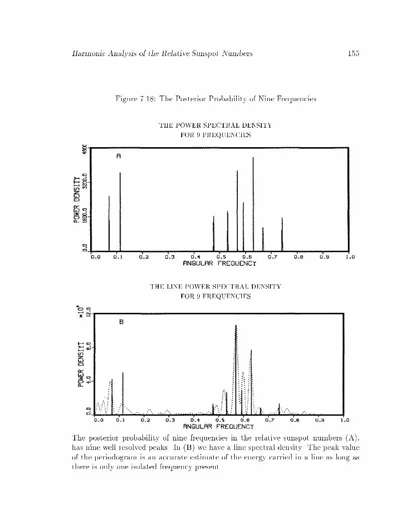
Harmonic Analysis of the Relative Sunspot Numbers 155
Figure 7.18: The Posterior Probability of Nine Frequencies
THE POWER SPECTRAL DENSITY
FOR 9 FREQUENCIES
THE LINE POWER SPECTRAL DENSITY
FOR 9 FREQUENCIES
The posterior probability of nine frequencies in the relative sunspot numbers (A),has nine well resolved peaks. In (B) we have a line spectral density. The peak valueof the periodogram is an accurate estimate of the energy carried in a line as long asthere is only one isolated frequency present.

156 CHAPTER 7
Figure 7.19: The Predicted Sunspot Series
THE ESTIMATED SUNSPOT NUMBERS
WOLF'S RELATIVE SUNSPOT NUMBERS
Not only can one obtain the estimated power carried by the signal, one can use theamplitudes to plot what probability theory has estimated to be the signal (A). Wehave included the relative sunspot numbers (B), for easy comparison.
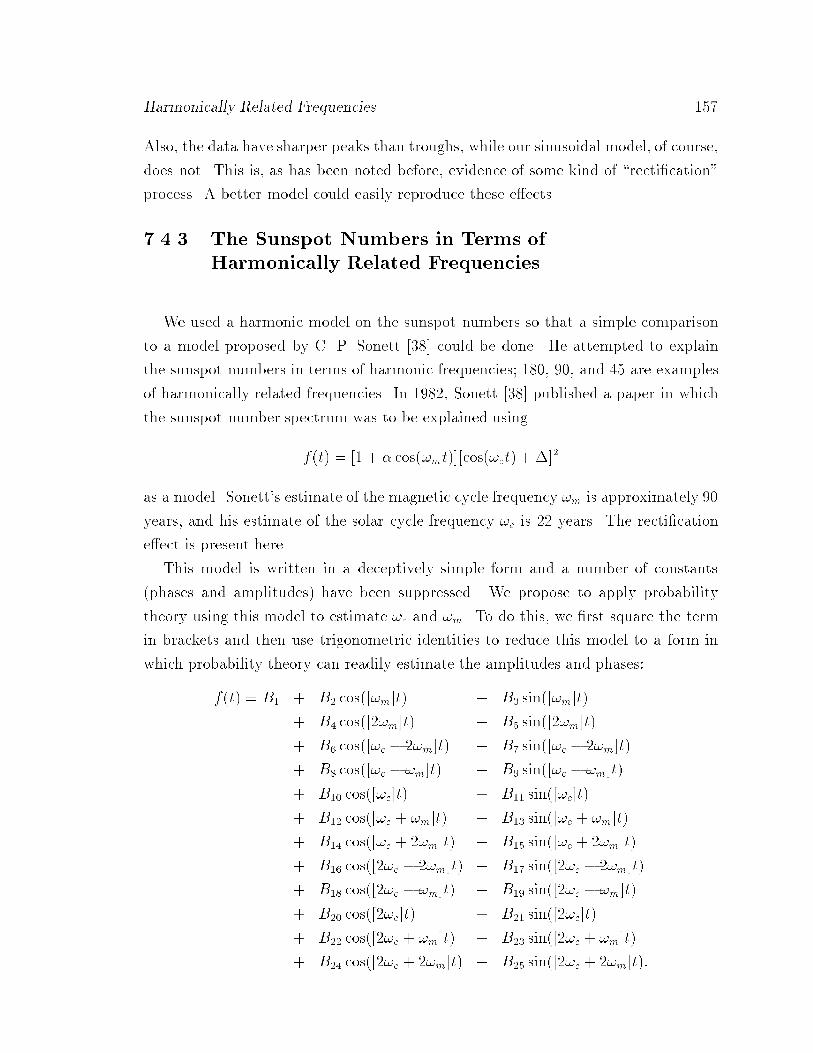
Harmonically Related Frequencies 157
Also, the data have sharper peaks than troughs, while our sinusoidal model, of course,
does not. This is, as has been noted before, evidence of some kind of \recti�cation"
process. A better model could easily reproduce these e�ects.
7.4.3 The Sunspot Numbers in Terms of
Harmonically Related Frequencies
We used a harmonic model on the sunspot numbers so that a simple comparison
to a model proposed by C. P. Sonett [38] could be done. He attempted to explain
the sunspot numbers in terms of harmonic frequencies; 180, 90, and 45 are examples
of harmonically related frequencies. In 1982, Sonett [38] published a paper in which
the sunspot number spectrum was to be explained using
f(t) = [1 + � cos(!mt)][cos(!ct) + �]2
as a model. Sonett's estimate of the magnetic cycle frequency !m is approximately 90
years, and his estimate of the solar cycle frequency !c is 22 years. The recti�cation
e�ect is present here.
This model is written in a deceptively simple form and a number of constants
(phases and amplitudes) have been suppressed. We propose to apply probability
theory using this model to estimate !c and !m. To do this, we �rst square the term
in brackets and then use trigonometric identities to reduce this model to a form in
which probability theory can readily estimate the amplitudes and phases:
f(t) = B1 + B2 cos([!m]t) + B3 sin([!m]t)
+ B4 cos([2!m]t) + B5 sin([2!m]t)
+ B6 cos([!c � 2!m]t) + B7 sin([!c � 2!m]t)
+ B8 cos([!c � !m]t) + B9 sin([!c � !m]t)
+ B10 cos([!c]t) + B11 sin([!c]t)
+ B12 cos([!c + !m]t) + B13 sin([!c + !m]t)
+ B14 cos([!c + 2!m]t) + B15 sin([!c + 2!m]t)
+ B16 cos([2!c � 2!m]t) + B17 sin([2!c � 2!m]t)
+ B18 cos([2!c � !m]t) + B19 sin([2!c � !m]t)
+ B20 cos([2!c]t) + B21 sin([2!c]t)
+ B22 cos([2!c + !m]t) + B23 sin([2!c + !m]t)
+ B24 cos([2!c + 2!m]t) + B25 sin([2!c + 2!m]t):

158 CHAPTER 7
Now Sonett speci�es the amplitudes of these, but not the phases [38]. We will take
a more general approach and not constrain these amplitudes. We will simply allow
probability theory to pick the amplitudes and phases which �t the data best. Thus
any result we �nd will have the Sonett frequencies !m and !c, but the amplitudes
and phases will be chosen in a way that will �t the data at least as well as does the
Sonett model { possibly somewhat better. After integrating out the amplitudes we
have only two parameters to determine, !c and !m.
We located the maximum of the posterior probability density using the computer
code in Appendix E and the pattern search routine. The \best" estimated value for
!c (in years) is approximately 21:0 years, and for !m approximately 643 years. The
values for these parameters given by Sonett are !c = 22 years and 76 < !m < 108
years with a mean value of !m � 89 years. Our probability analysis estimates the
values of !c to be about the same, and !m to be substantially di�erent, from those
given by Sonett. The most indicative value is the estimated standard deviation for this
model: �Sonett = 25:5 years. By this criterion, this model is no better than a four-
frequency model. Considering that a four-frequency model has 15 degrees of freedom
compared to 29 for this model, we can all but exclude harmonically related frequencies
as a possible explanation of the sunspot numbers. Of course, these conclusions refer
only to an analysis of the entire run of data; if we considered the �rst century of the
record to be unreliable and analyzed only the more recent data, a di�erent conclusion
might result.
7.4.4 Chirp in the Sunspot Numbers
We have so far investigated two variations of harmonic analysis of the relative
sunspot numbers. Let us proceed to investigate a more complex case to see whether
there is more structure in the relative sunspot numbers than just simple periodic
behavior. These data have been looked at from this standpoint at least once before.
Bracewell [39] has analyzed these numbers to determine whether they could have a
time-dependent \instantaneous phase". The model used by Bracewell can be written
as
f(t) = B1 +Re [E(t) exp(i�(t) + i!11t)]
where B1 is a constant term in the data, E(t) is a time varying magnitude of the
oscillation, �(t) is the \instantaneous phase", and !11 is the 11 year cycle.
Chirp in the Sunspot Numbers 159
This model does not incorporate any prior information into the problem. It is so
general that any function can be written in this form. Nevertheless, the idea that the
phase �(t) could be varying slowly with time is interesting and worth investigating.
An \instantaneous phase" in the notation we have been using is a chirp. Let �(t)
stand for the phase of the signal, and ! its frequency. Then we may Taylor expand
�(t) around t = 0 to obtain
!t+ �(t) � �0 + !t+�00
2t2 + � � � ;
where we have assumed �0(t) = 0. If this were not so then ! is not the frequency as
presumed here. The Bracewell model can then be approximated as
f(t) = B1 + E(t)[cos(!t+ �t2) +B2 sin(!t+ �t2)]:
Thus, to second order, the Bracewell model is just a chirped frequency with a time
varying envelope.
We can investigate the possibility of a chirped signal using
f(t) = C1 + C2 cos(!t+ �t2) + C3 sin(!t+ �t2)
as the model, where � is the chirp rate, C1 is a constant component, ! is the frequency
of the oscillation, and C2 and C3 are e�ectively the amplitude and phase of the
oscillation. This model is not a substitute for the Bracewell model. Instead this
model is designed to allow us to investigate the possibility that the sunspot numbers
contain evidence of a chirp, or \instantaneous phase" in the Bracewell terminology.
A plot of the log of the \Student t-distribution" using this model is the proper
statistic to look for chirp. However, we now have two parameters to plot, not one.
In Fig.7.20 we have constructed a contour plot around the 11 year cycle. We expect
this plot to have a peak near the location of a frequency. It will be centered at zero
chirp rate if there is no evidence for chirp, and at some nonzero value when there is
evidence for chirp. Notice, that along the line � = 0 this \Student t-distribution" is
just the simple harmonic probability distribution studied earlier, see Fig. 2.1(A). As
with the Fourier transform if there are multiple well separated chirped frequencies
(with small chirp rates) then we expect there to be multiple peaks in Fig. 7.20.
There are indeed a number of peaks; the single largest point on the plot is located
o� the � = 0 axis. The data contain evidence for chirp. The low frequencies also
show evidence for chirp. To the extent that the Bracewell \instantaneous phase" may
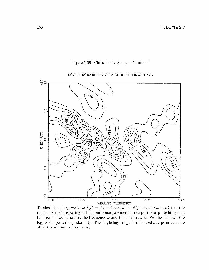
160 CHAPTER 7
Figure 7.20: Chirp in the Sunspot Numbers?
LOG10 PROBABILITY OF A CHIRPED FREQUENCY
To check for chirp we take f(t) = A1 + A2 cos(!t + �t2) + A3 sin(!t + �t2) as themodel. After integrating out the nuisance parameters, the posterior probability is afunction of two variables, the frequency ! and the chirp rate �. We then plotted theloge of the posterior probability. The single highest peak is located at a positive valueof �: there is evidence of chirp.

7.5. MULTIPLE MEASUREMENTS 161
be considered as a chirp, we must agree with him: there is evidence in these data for
chirp.
In light of this discussion, exactly what these numbers represent and exactly what
is going on inside the sun to produce them must be reconsidered. The orthogonal ex-
pansion on these numbers indicates that the complexity of these numbers is immense
and no simple model will su�ce to explain them. Given the total number of degrees
of freedom it is likely that every cycle has a unique amplitude and a complex non-
sinusoidal shape. In other words, di�erent sunspot cycles are about as complicated
in structure as are di�erent business cycles in economic data. If that is true, the
only frequency in these data of any relevance is probably the 11 year cycle; the other
indications of frequency are just e�ects of the nonharmonic oscillation. Again, had
we analyzed only the more recent data, the conclusions might have been di�erent.
Certainly we have not answered any real questions about what is going on; indeed
that was not our intention. Instead we have shown how use of probability theory
for data analysis can facilitate future research by testing various hypotheses more
sensitively than could the traditional intuitive ad hoc procedures.
7.5 Multiple Measurements
The traditional way to analyze multiple (i.e. multi-channel) measurements is to
average the data, and then analyze the averaged data. The hoped-for improvement
in the parameter estimates is the standardpn rule. To derive this rule one must
assume that the signal and the noise variance, are the same in every data set, and
that the noise samples were uncorrelated. Unfortunately, the conditions under which
averaging works at its theoretical best are almost never realized in real experiments.
Speci�cally, all experiments contain some e�ects which will not average out. These
e�ects can become so signi�cant, that the evidence for the signal can be greater in
any one of the data sets that went into the average than it is in the averaged data (we
will demonstrate this shortly). There are three main reasons why averaging may fail
to give the expectedpn improvement in the parameter estimates: the experiment
may not be reproducible, the model may incorrect, the noise within di�erent data
sets may be correlated.
In real physics experiments, reproducibility depends critically on the electronics
repeating itself exactly every time. Of course this never happens; there are always
162 CHAPTER 7
small di�erences. For example, to repeat an NMR experiment one must bring the
sample to a stationary state (this may be far from equilibrium) and then further excite
the sample using a high power radio transmitter. In a perfect world, every time one
excited the sample it would be with a pulse of exactly the same amplitude and exactly
the same shape as before. Of course this never happens; every repetition is a unique
experiment having slightly di�erent amplitudes, phases, and noise variance. These
slight di�erences are enough to cause averaging to fail to give thepn improvement
when large numbers of data sets are averaged, even when the noise samples are
independent.
The second source of systematic error is in our imprecise knowledge of the model.
If the signal is exactly the same in each data set, of course the noise is reduced by
averaging. Unfortunately, if we do not know the model exactly, then our model is only
an approximation. When we �t the model to the data, some of the \true" signal will
not be �t. This mis�t of the model will be called noise by probability theory. But it
is noise that is perfectly correlated in successive data sets, and does not average out.
Thus the accuracy estimates will not improve, because the dominant contribution to
the estimated noise variance will be the mis�t between the model and the data.
If any systematic e�ect is present, averaging will fail to give the expected improve-
ment; nevertheless, probability theory does not mislead us. We have stressed several
times that the estimates one obtains from these procedures are conservative. That is,
when the models mis�t the data they still give the best estimates of the parameters
possible under the circumstances, and yield conservative (wide) error estimates. This
suggests that by analyzing each data set separately, and looking for common e�ects,
we might be able to realize better estimates than by averaging. In this section we
investigate the e�ects of multiple measurements and compare the results of a joint
analysis (analyzing all of the data) to the analysis of the averaged data. We will do
this analysis on a data set that most people would not hesitate to average. This is our
�rst example where we apply Bayesian analysis to data which are not a time series.
The experiment we will consider is a simple di�raction experiment. A mercury
vapor lamp was placed in front of a slit, and the light from the lamp passed through
the slit and onto a screen. An electronic camera (a Charge Coupled Device { CCD)
was placed behind the screen and used to image the intensity variations. The data
for this analysis were kindly provided by W. H. Smith [41]. The image consists of
a series of light and dark bars typical of such experiments. The pattern for the �rst
row in the CCD is shown in Fig. 7.21(A). Figure 7.21(B) is a plot of the averaged
The Averaging Rule 163
data.
This particular device has 573 pixels in each row and there are 380 rows. Thus there
are a total of 380 repeated measurements. The CCD was aligned parallel with the slit,
so the image appearing in each row should be identical. In principle the data could
be averaged to obtain ap380 improvement in the parameter estimates. However, the
concerns mentioned earlier are all applicable here. The types of systematic e�ects that
can enter this experiment are numerous, but a few of them are: the camera readout
has small systematic variations from one row to the next; there can be intensity
variations from the �rst to last row; and if the alignment of the camera is not perfect,
there will be small phase drifts from the �rst to last row. Nonetheless, when one
looks at these data, there is absolutely no reason to believe that averaging should not
work.
We begin the analysis by plotting the log10 of the probability of a single harmonic
frequency plus a constant. We plot this probability density for the �rst row of the CCD
in Fig. 7.22(A), for the average of the 380 data sets in Fig. 7.22(B), and jointly for all
data Fig. 7.22(C). One sees from the average data, Fig. 7.22(B), that there is indeed
large evidence for a frequency near 1.6 in dimensionless units. That peak is some 133
orders of magnitude above the noise level. The second thing that one sees is that the
peak from the �rst row of the CCD, Fig. 7.22(A), is some 136 orders of magnitude
above the noise: the peak from one row has more evidence for frequencies than the
average data! The third plot, Fig. 7.22(C), is from the joint analysis. That peak is
some 55,000 orders of magnitude higher than the average data! The implications of
this are indeed staggering. If one cannot average data in an experiment as simple as
this one, then there are probably no conditions under which averaging is the way to
proceed. Because the issues raised by this simple example are so important, we will
pause to investigate some of the theoretical implications before proceeding with this
example.
7.5.1 The Averaging Rule
To derive the average rule one assumes a signal f(t), and n sets of data d(ti)j with
noise variance �2. The signal f(t) and the noise variance �2 are assumed to be the
same in every data set. Then the probability that we should obtain a data set d(ti)j
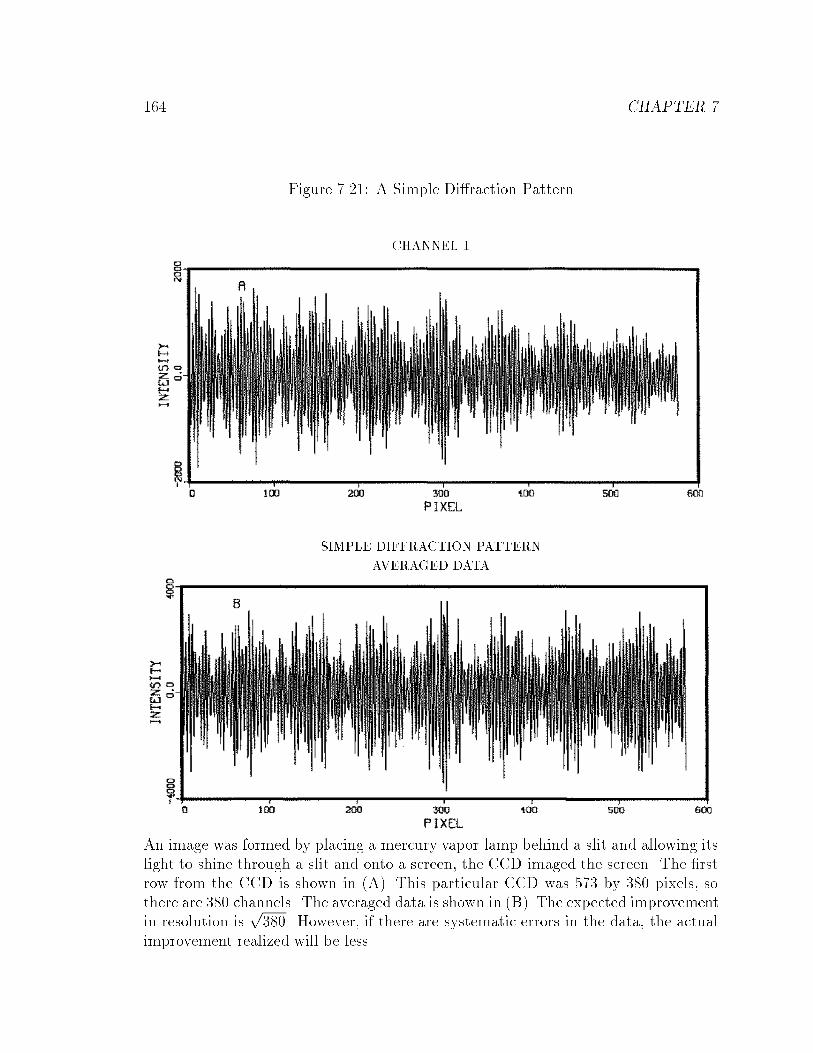
164 CHAPTER 7
Figure 7.21: A Simple Di�raction Pattern
CHANNEL 1
SIMPLE DIFFRACTION PATTERN
AVERAGED DATA
An image was formed by placing a mercury vapor lamp behind a slit and allowing itslight to shine through a slit and onto a screen, the CCD imaged the screen. The �rstrow from the CCD is shown in (A). This particular CCD was 573 by 380 pixels, sothere are 380 channels. The averaged data is shown in (B). The expected improvementin resolution is
p380. However, if there are systematic errors in the data, the actual
improvement realized will be less.
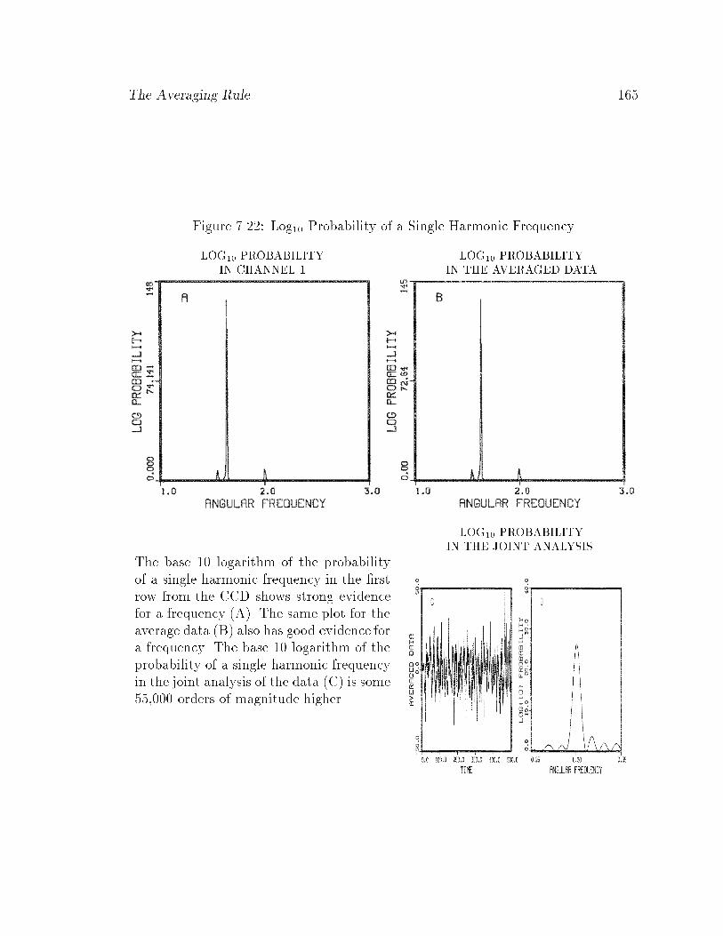
The Averaging Rule 165
Figure 7.22: Log10 Probability of a Single Harmonic Frequency
LOG10 PROBABILITY
IN CHANNEL 1
LOG10 PROBABILITY
IN THE AVERAGED DATA
The base 10 logarithm of the probabilityof a single harmonic frequency in the �rstrow from the CCD shows strong evidencefor a frequency (A). The same plot for theaverage data (B) also has good evidence fora frequency. The base 10 logarithm of theprobability of a single harmonic frequencyin the joint analysis of the data (C) is some55,000 orders of magnitude higher.
LOG10 PROBABILITY
IN THE JOINT ANALYSIS

166 CHAPTER 7
is given by
P (Dj jf; �; I) / exp
(� 1
2�2
NXi=1
(d(ti)j � f(ti))2
):
If the noise samples in di�erent channels are independent, the probability that we
should obtain all the data sets is just the product of the probabilities that we should
obtain any one of the data sets:
P (Djf; �; I) / �nj=1 exp
(� 1
2�2
NXi=1
(d(ti)j � f(ti))2
):
This can be written as
P (Djf; �; I) / exp
(� n
2�2
NXi=1
[d(ti)2 � 2d(ti)f(ti) + f(ti)2]
);
where d(ti)2 is the mean square data value at time ti, and d(ti) is the mean data value,
where \mean" signi�es \average over the channels". This is almost a standard model-
�tting problem with the data replaced by the average. The procedure is called \Brute
Stacking" by geophysicists. The improvement comes from the factor of n multiplying
the term in square brackets. We demonstrated that the accuracy estimates are all
proportional to the square root of the variance, and here the variance is e�ectively
�2=n { this gives the standardpn improvement.
7.5.2 The Resolution Improvement
When multiple data sets are analyzed jointly, how much improvement in the pa-
rameter estimates can be expected? The resolution improvement depends on the
curvature of the posterior probability density at the maximum. The general rule de-
pends on the model; all we can say is that if all of the data sets have approximately
the same evidence in them, then the logarithm of the posterior probability density
is n times larger and something like thepn improvement will be realized. We can
demonstrate this for the single frequency estimation problem. Then the posterior
probability of the frequency, given n repeated measurements and assuming the noise
variance �2 is the same, is
P (!j�;D; I) � exp
8<:
nXj=1
C(!)j�2
9=; (7:4)
Signal Detection 167
where C(!)j is the Schuster periodogram evaluated for data set j. To obtain the
accuracy estimates we expand the exponent about the \true" frequency ! to obtain
P (!jD; I) � exp
8<:�
nXj=1
bj(! � !)2
2�2
9=; ;
where bj = �C 00j for the jth data set. If the data contain a single sinusoid such as
B cos(!t), then b is given by Eq. (2.10). This gives the posterior probability density
for a simple harmonic frequency when multiple measurement are present as
P (!jD; I) � exp
8<:�
nXj=1
N3B2j
96�2(! � !)2
9=; :
The accuracy estimate is given by
(!)est = ! �s
48�2
N3nB2
where B2 is the mean square of the true amplitude. If all of the amplitudes are nearly
the same height, this is just the standardpn improvement.
The improvement realized is directly related to how well the assumptions in the
calculation are met. In the case of averaging, the assumptions are that the amplitude,
frequency, phase, and noise variance are the same in every data set. For the example
just given we removed the assumption that the amplitudes had to be the same in
every data set, consequently, nB2 was replaced by nB2. If we further remove the
assumption that the noise variance is the same in every data set, then nB2 is replaced
byPn
j=1 B2j =�
2j .
When the assumed conditions are not met, the price one pays is in resolution. The
procedure described by Eq. (7.2) is more general than averaging in that it allows the
amplitudes, phases, and noise variance to be di�erent for each data set and still allows
one to look for common e�ects. When the true amplitudes, phases, and noise variance
are the same in every data set this procedure reduces to averaging. Thus Eq. (7.2)
represents a more conservative approach than averaging and will realize something
approaching thepn improvement under a wider variety of conditions, because it
makes fewer assumptions.
7.5.3 Signal Detection
When multiple measurements are present we would like to understand what hap-
pens to the joint analysis as we increase the number of measurements. In other words
168 CHAPTER 7
we typically average data when the signal-to-noise ratio is very bad. We do this be-
cause we think it allows one to reduce the noise; thus small signals can be detected.
But what will happen with the joint analysis? The general answer for the joint anal-
ysis again depends on the model function. However, as noted earlier, if the evidence
in each data set is roughly the same the su�cient statistic will be n times larger than
when only a single measurement is present. Thus the evidence for a signal will build
up in a manner similar to averaging. We will demonstrate how the evidence accumu-
lates in the joint analysis using the single frequency model. The posterior probability
density of a common harmonic frequency, when multiple measurements are available,
is again given by Eq. (7.4). What we would like to know is how high is the peak in
Eq. (7.4)? Again taking the data to be
d(t)j = Bj cos(!t)
the peak value of the periodogram is given approximately by
C(!)j �NB2
j
4:
Assuming each data set has the same number of data values N , the maximum of the
posterior probability density will be
P (!jD; I) / exp
8<:
nXj=1
NB2j
4�2
9=; :
We can simplify this by usingnXj=1
B2j = nB2
where B2 is the mean-square true amplitude. The evidence for a signal increases by
the power of the number of data sets:
P (!jD; I) / exp
(nNB2
4�2
):
If we allow the variance of the noise to be di�erent in each data set nB2 will be
replaced by a weighted averagePn
j=1 B2j =�
2j . Again we �nd the height of the posterior
probability density depends directly on the assumptions made in the calculation. In
the case of averaging, the log-height of the posterior probability density is n times
larger than the height from one data set (provided the assumptions are met). If we
relax the assumptions about the amplitude B, we replace B2 in the average rule by

The Distribution of the Sample Estimates 169
the mean-square true value. If we further relax the assumptions and allow the noise
variances to be di�erent, we obtain the weighted average of the true B2 values. Thus
we again have a more conservative procedure that will reduce to give thepn rule when
the appropriate conditions are met, under much wider conditions than averaging. In
the case of the simple harmonic frequency, doubling the number of data sets is similar
to doubling the number of time samples, while keeping the total sampling time �xed.
This is not the best way to �nd a signal (doubling the signal-to-noise works better),
but if no other course is available it will build up the probability density by essentially
squaring the distribution for each doubling of the number of data sets.
7.5.4 The Distribution of the Sample Estimates
In the CCD example, we had 380 repeated measurements, and the maximum of
the posterior probability was some 55,000 orders of magnitude above the noise. Each
data set raised the posterior probability approximately 55,000/380 = 144 orders of
magnitude. But when the data were averaged, small variations in the amplitude,
phases, and variance of the noise caused systematic variations in the data which
were nonsinusoidal. Probability theory automatically reduced both the height of the
posterior density (i.e. it could not see the signal as well) and reduced the precision of
the estimates. In this example the height was reduced from 55,000 to 133, and the
accuracy was reduced from 6:8� 10�8 to 0.00036; the error estimate of the averaged
data is 5266 times larger than the estimate from the joint analysis. It thus appears
that data averaging (Brute Stacking) is never better than a joint analysis of the
data, and it is in general worse. Averaging does, of course, reduce the amount of
computation; but with modern computers this is not an important consideration.
In this last example the improvement was very dramatic, but this was real exper-
imental data; perhaps the reason averaging failed was some other e�ect in the data.
We would like to show that the cause was the variation of the signal and the noise
variance in the various data sets. To do this we will generate data from the following
equation
d(t) = B cos(0:3t+ �) + e(t): (7:5)
We will vary B, �, and � from one data set to another. We will then estimate the
frequency in the averaged data and in a joint analysis of all the data, and show that
these variations will cause averaging to fail to give thepn improvement; while a joint
analysis will continue to exhibit the expected improvement.

170 CHAPTER 7
We generated multiple data sets from Eq. (7.5). Each data set we generated had a
di�erent amplitude B, phase �, and noise variance �2. To generate the data we used
three Gaussian random numbers with unit variance. We used one as the amplitude
B, another as the phase �, and the third to scale the noise. The noise was generated
using a Gaussian random number generator with unit variance. We generated the
noise and then multiplied it by the third random number. Using this procedure, the
signal will average to zero.
We generated 100 data sets, each containing 512 data values. An example of
one such data set is shown in Fig. 7.23(A). The log10 of the probability of a single
harmonic frequency is shown in Fig. 7.23(B). We have also displayed the average
data Fig. 7.23(C) and the log10 probability of a single frequency. In this particular
case averaging has not completely cancelled the signal, however, one measurement,
Fig. 7.23(A), has about a 109 times more evidence for a signal than the average data,
Fig. 7.23(B). We estimated the frequency in the 100 data sets in a joint analysis and
in the averaged data. We then selected three new random numbers and repeated this
calculation 3000 times.
The results are summarized in Table 7.2. This table contains the actual estimates
from a few of the 3000 sets of data analyzed. The second column is the estimated
frequency from the average data. The third column is the squared di�erence between
the true frequency and the estimate from the averaged data, (the variance of this esti-
mate). The fourth column is the estimated frequency from the joint analysis, and the
�fth column is the squared di�erence between the true frequency and the estimated
frequency from the joint analysis. We averaged all 3000 entries (labeled average at
the bottom of the table), and we computed the square root (the standard deviation)
estimate for the variance (columns 3 and 5). The estimate from the averaged is a
little better than it actually was in these data. When we estimated the frequency we
had to give the search routine an initial estimate of the frequency. This locked the
search routine onto the correct peak in the periodogram even though there was no
clear peak in many of the data sets. This is analogous to estimating the averaged
frequency with a strong prior.
For a single data set with unit signal-to-noise the \best" estimated frequency
should be �0:0006 radians per step; the estimated standard deviation of the aver-
aged data is about a factor of 2 larger than what one would obtain from one data
set. Thus averaging has destroyed evidence in the data: any one data set contains
more evidence for frequencies than the averaged data. If averaging were working

The Distribution of the Sample Estimates 171
Figure 7.23: Example { Multiple Measurements
ONE OF 100 DATA SETSLOG10 PROBABILITY
OF ONE FREQUENCY
THE AVERAGED DATALOG10 PROBABILITY
OF ONE FREQUENCY
We generated 100 such data sets with di�erent amplitude, phase, and noise variance,but the same frequency (see text for details). In (A) we have displayed one such dataset. The log10 of the probability of a single harmonic frequency is displayed in (B).The average data (C) and the log10 probability of a single frequency in (D) show 10�9
times less evidence for a harmonic frequency than one data set.

172 CHAPTER 7
Table 7.2: \Brute Stacking" vs. Joint AnalysisFrequency Estimate (h!i � 0:3)2 Frequency Estimate (h!i � 0:3)2
Average Joint Analysis1 0:30018 3:52�8 0:2999974 6:81�12
2 0:29863 1:87�6 0:2999896 1:08�10
3 0:29987 1:47�8 0:2999782 4:75�10
4 0:30076 5:79�7 0:2999995 1:64�13
5 0:30044 2:00�7 0:2999881 1:42�10
6 0:29804 3:82�6 0:2999998 2:78�14
7 0:30024 5:77�8 0:2999995 1:64�13
8 0:30047 2:22�7 0:2999985 2:18�12
9 0:29966 1:09�7 0:2999985 2:18�12
10 0:29990 8:30�9 0:3000088 7:90�11
......
......
...2999 0:30152 2:31�6 0:2999969 9:16�12
3000 0:29968 1:02�7 0:3000008 7:16�13
Average 0:29999 1:39�6 0:2999995 3:02�11
SD 1:17�3 5:49�6
We generated 3000 frequency estimates (see text for details). The frequency estimatein the second column was from the averaged data, and the third column is the variancefor that estimate. The fourth and �fth columns are the estimates from the jointanalysis. The row labeled \Average" is the average of the 3000 frequency and varianceestimates. The last row is the square root of the average variance. Averaging actuallyappears a little better than it is in these data: when we estimated the frequency wehad to supply an initial frequency estimate; this locked the search routine onto thecorrect peak in the periodogram, even though there was no clear peak above the noisein many of the averaged data sets. From a probability standpoint this is analogousto estimating the average frequency with a strong prior.

Example { Multiple Measurements 173
at its theoretical best we would expect that in 100 data sets the estimates should
improve to �0:0006=p100 = �0:00006 radians per step. Averaging is a factor of
20 times worse than it should be. But how has the joint analysis done? For 3000
such estimates (in unit signal-to-noise) the joint analysis can do no better than thepn rule: �0:00006=
p3000 � �0:000001 radians per step, where we �nd �0:000005,
about a factor of 5 larger; we conclude that the mean square weighted amplitude
was about 1/25. The joint analysis has performed well; about 0:001=0:000005 = 185
times better than averaging.
From the 3000 frequency estimates we computed a cumulative distribution of the
number of estimates within one standard deviation, two deviations etc. of the true
This distribution is displayed in Fig. 7.24. The solid line is the cumulative sample
distribution, while the dashed line is the equivalent plot for a Gaussian having the
same mean and standard deviation as the sample. The estimates resemble a Gaussian,
but there are systematic di�erences. These di�erences are numerical in origin. We had
to locate the maximum of the posterior probability, and this distribution is roughly
100 times more sharply peaked than a discrete Fourier transform. The pattern search
routine we used moves the frequency by some prede�ned �xed amount. Typically it
will move the frequency by only one or two steps, this tends to bunch the estimates
up into discrete categories. We could �x this problem at the cost of much greater
computing time.
7.5.5 Example { Multiple Measurements
We started this section by presenting a simple di�raction experiment and became
sidetracked by some of the implications of the example. When we computed the
su�cient statistic of the joint analysis we found the peak to be some 55,000 orders of
magnitude higher than the peak for the averaged data. We have used the estimate
of the frequency from that peak in several places; here, we plot the results of that
analysis to give a better understanding of the determination of the frequency. We will
estimate the frequency from the periodogram of the averaged data, from the \Student
t-distribution" using the averaged data, and last using a joint analysis on all of the
data.
The results of this analysis are displayed in Fig. 7.25. The normalization on all
of these curves is arbitrary. If we took the periodogram of the averaged data as our
frequency estimate we would have the broad peak in Fig. 7.25. However, probability

174 CHAPTER 7
Figure 7.24: The Distribution of Sample Estimates
We generated 100 data sets with di�erent amplitude, phase, and noise variance butthe same frequency. From the 100 data sets we estimated the frequency. We thengenerated another 100 data sets and estimated the frequency. We repeated thisprocess some 3000 times. Here we have plotted the cumulative percentage of estimates(solid line) falling within one, two, and three RMS standard deviations. The dashedline is the equivalent distribution for a Gaussian. The axis labels here correspond totwo, four, and six standard deviations.
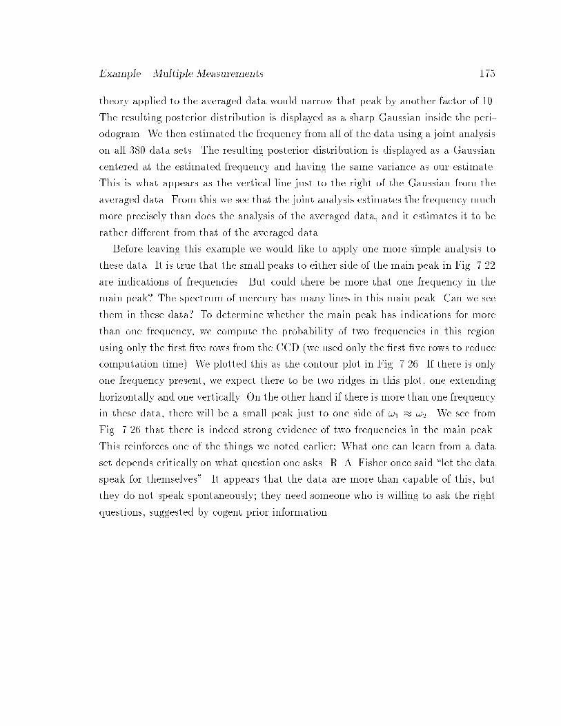
Example { Multiple Measurements 175
theory applied to the averaged data would narrow that peak by another factor of 10.
The resulting posterior distribution is displayed as a sharp Gaussian inside the peri-
odogram. We then estimated the frequency from all of the data using a joint analysis
on all 380 data sets. The resulting posterior distribution is displayed as a Gaussian
centered at the estimated frequency and having the same variance as our estimate.
This is what appears as the vertical line just to the right of the Gaussian from the
averaged data. From this we see that the joint analysis estimates the frequency much
more precisely than does the analysis of the averaged data, and it estimates it to be
rather di�erent from that of the averaged data.
Before leaving this example we would like to apply one more simple analysis to
these data. It is true that the small peaks to either side of the main peak in Fig. 7.22
are indications of frequencies. But could there be more that one frequency in the
main peak? The spectrum of mercury has many lines in this main peak. Can we see
them in these data? To determine whether the main peak has indications for more
than one frequency, we compute the probability of two frequencies in this region
using only the �rst �ve rows from the CCD (we used only the �rst �ve rows to reduce
computation time). We plotted this as the contour plot in Fig. 7.26. If there is only
one frequency present, we expect there to be two ridges in this plot, one extending
horizontally and one vertically. On the other hand if there is more than one frequency
in these data, there will be a small peak just to one side of !1 � !2. We see from
Fig. 7.26 that there is indeed strong evidence of two frequencies in the main peak.
This reinforces one of the things we noted earlier: What one can learn from a data
set depends critically on what question one asks. R. A. Fisher once said \let the data
speak for themselves". It appears that the data are more than capable of this, but
they do not speak spontaneously; they need someone who is willing to ask the right
questions, suggested by cogent prior information.

176 CHAPTER 7
Figure 7.25: Example - Di�raction Experiment
The broad curve on this graph is the periodogram from the averaged data. The sharpGaussian inside this line is the posterior distribution obtained from the averaged data.The sharp spike located just o�-center is the Gaussian representing the posteriordistribution from all 380 data sets.
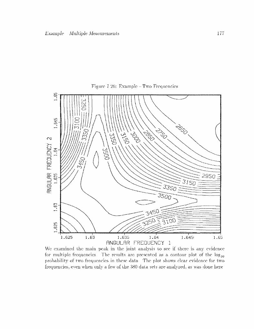
Example { Multiple Measurements 177
Figure 7.26: Example - Two Frequencies
We examined the main peak in the joint analysis to see if there is any evidencefor multiple frequencies. The results are presented as a contour plot of the log10probability of two frequencies in these data. The plot shows clear evidence for twofrequencies, even when only a few of the 380 data sets are analyzed, as was done here.

178 CHAPTER 7
Chapter 8
SUMMARY AND
CONCLUSIONS
In this study we have attempted to develop and apply some of the aspects of
Bayesian parameter estimation to time series, even though the analysis as formulated
is applicable to any data set, be it a time series or not.
8.1 Summary
We began this analysis in Chapter 2, by applying probability theory to estimate the
spectrum of a data set that, we postulated, contained only a single sinusoid plus noise.
In Chapter 3, we generalized these simple considerations to relatively complex models
including the problem of estimating the spectrum of multiple nonstationary harmonic
frequencies in the presence of noise. This led us to the \Student t-distribution": the
posterior probability of the f!g parameters, whatever their meaning. In Chapter 4,
we estimated the parameters and calculated, among other things, the power spectral
density, and the noise variance, and we derived a procedure for assessing the accuracy
of the f!g parameter estimates. In Chapter 6, we specialized to spectrum analysis
and explored some of the implications of the \Student t-distribution" for this prob-
lem. In Chapter 7, we applied these analyses to a number of real time series with
the aim of exploring and broadening some of the techniques needed to apply these
procedures. In particular, we demonstrated how to use them to estimate multiple
nonstationary frequencies and how to incorporate incomplete information into the
estimation problem.
179

180 CHAPTER 8
8.2 Conclusions
Perhaps the single biggest conclusion of this work is that what one can learn about
a data set depends critically on what questions one asks. If one insists on taking the
discrete Fourier transform of a data set, then our analysis shows that one will always
obtain good answers to the question \What is the evidence of a single stationary
harmonic frequency in these data?" This will be adequate if there are plenty of data
and there is no evidence of complex phenomena. However, if the data show evidence
for multiple frequencies or complex behavior, the discrete Fourier transform can give
misleading or incorrect results in the light of more realistic models.
Although the use of integration to remove nuisance parameters is not new, and
indeed the calculation in Chapter 3 has, to some degree, been done by every Bayesian
who ever removed a nuisance parameter by integration, the realization of the degree
of narrowing of the marginal joint posterior probability density that can be achieved
by this is, to the best of our knowledge, new and almost startling. It indicates
that, even though we might not be able to estimate an amplitude very precisely, the
f!g parameters often associated with an amplitude may be very precisely estimated.
We can often improve the estimation of frequencies and decay rates by orders of
magnitude over the estimates obtained from the discrete Fourier transform, least
squares, or maximum likelihood. This is not to say that the actual estimates will
be very di�erent from those obtained from maximum likelihood or least squares {
indeed, when little prior information is available the estimates of the parameters are
the maximum likelihood estimates. The major di�erence is in the indicated accuracy
of the estimates.
The principles of least squares or maximum likelihood provide no way to eliminate
nuisance parameters, and thus oblige one to seek a global maximumin a space of much
high dimensionality, which typically requires orders of magnitude more computation
time. Having found this, they provide no way to assess the accuracy of the estimates
other than the sampling distribution of the estimator { which is another even longer
calculation. But it is a calculation that does not answer the real question of interest;
it answers the \pre-data" question:
(Q1): \Before you have seen the data, how much do you expect the estimate to
deviate from the true parameter value?"
The question of interest is the \post-data" one:

Conclusions 181
(Q2): \After getting the data, how accurately does the data set that you actually
have determine the true values of the parameters?"
That these are very di�erent questions with di�erent answers in general, was rec-
ognized already by R. A. Fisher in the 1930's; he noted that in general two data sets
that yield the same numerical value of the estimator, may nevertheless justify very
di�erent claims of accuracy. He sought to correct this by his device of conditioning on
\ancillary statistics." But Jaynes [42] then showed that this conditioning is mathe-
matically equivalent to using Bayes' theorem, as we have done here. Bayes' theorem,
of course, always answers question (Q2), whether or not ancillary statistics exist.
The procedures for comparing models, Eq. (5.9), are perhaps new in the sense
that we have extended the Bayesian calculation into the nonlinear f!g parameters
and by carefully keeping track of the normalization constants we were able eventually
to integrate out all the parameters. This gives an objective way to compare models
and to determine when additional e�ects are present in the data. Of course, as with
any calculation, it will never replace the good sound judgment of the experimenter.
The calculation can give a relative ranking of the various choices presented to it. It
cannot decide which models to test.
Last, the improvement realized by these procedures when multiple measurements
are present is quite striking. The analysis presented in Chapter 7 indicates that
the traditional averaging rule will hold whenever the signal is exactly the same in
every measurement. Yet in real experiments it is almost impossible to realize the
true theoretical improvement. However, by computing the joint marginal posterior
probability density of the common e�ects, the expectedpn can be obtained even
in data sets where averaging clearly will not work. The implications of this for
NMR and other �elds are rather profound. Using these techniques we were able
to improve resolution in NMR experiments by several orders of magnitude over the
discrete Fourier transform; this is making it possible to examine extremely small
e�ects that could not be examined before.

182 CHAPTER 8

Appendix A
Choosing a Prior Probability
The question \How to choose the prior probability to express complete ignorance?"
is interesting in itself, and it cannot be evaded in any problem of scienti�c inference
that is to be solved by using probability theory and Bayes' theorem, but in which we
do not wish to incorporate any particular prior information. In the case of the simple
harmonic analysis performed in Chapter 2, there are four parameters to be estimated
(B1, B2, !, �), and it is not obvious which choice of prior probabilities is to be pre-
ferred. Presumably, any prior probability distribution represents a conceivable state
of prior information, but the problem of relating the distribution to the information is
subtle and open-ended. You can always think more deeply and thus dredge up more
prior information that you didn't think to use at �rst.
There are two questions one may consider to help in this. First, one should ask
\Are the parameters logically connected?" That is, if we gain additional information
about one of the parameters, does it change the estimates we would make about the
others? If the answer is yes, then the parameters are not logically independent. It
will be useful to �nd a representation where the parameters are independent.
Another useful question is \What are the invariances that the prior probability
must obey?" That is, what transformations would convert the present problem into
one where we have the same state of prior knowledge? Actually it is only this sec-
ond question that is truly essential. However, using a representation in which the
parameters are not logically independent will mean that the prior probabilities for
all the parameters must be determined at once, by utilizing the properties of all the
parameters.
In the two representations considered in Chapter 2, Cartesian versus polar, ob-
taining information about the frequency would rarely a�ect one's prior estimates of
183
184 APPENDIX A
the phase, amplitude, and noise level. Then the prior for the frequency will be in-
dependent of the other parameters, and the only invariance to be considered is some
group of mappings S of ! onto itself. Later in this appendix we will derive the prior
from the group of scale changes.
In the Cartesian representation, B1 and B2 are usually logically independent in
the sense just noted, so we would assign them independent priors. In the polar
notation the amplitude and phase are also logically independent, because obtaining
information about either would not a�ect our prior estimate of the other. The volume
elements transform as
dB1dB2 = BdBd�
and so we want a probability density � with the two seemingly di�erent forms:
�(B1; B2)dB1dB2 = �(B; �)BdBd�
with
�(B1; B2) = f(B1)f(B2)
but also
�(B; �) = g(B)h(�):
But we rarely have prior information about �, so we should take h(�) = const = 1=2�,
(0 � � � 2�). We are left with
f(B1)f(B2) =1
2�g(qB2
1 +B22)
but setting B2 = 0, this reduces to
f(B1)f(0) =1
2�g(B1)
so we have the functional equation
f(x)f(y) = f(qx2 + y2)f(0)
which a reasonable prior must satisfy. By writing this as
log[f(x)] + log[f(y)] = log[f(qx2 + y2)] + log[f(0)]
the general solution is obvious; if a function l(x) plus a function l(y) is a constant
plus a function only of (x2 + y2) for all x, y the only possibility is
l(x) = ax2 + b:

Choosing a Prior Probability 185
Thus, f(x) must be a Gaussian; with a = �1=2�2 (the value of b is determined by
normalization):
f(x) =1p2��2
exp
(� x2
2�2
):
To a modern physicist, this argument seems very familiar; it is just a two-dimensional
version of Maxwell's original derivation of the Maxwellian velocity distribution [43].
However, historical research has shown that the argument was not original with
Maxwell; ten years earlier the astronomer John Herschel [44] had given just our two-
dimensional argument in �nding the distribution of errors in measuring the position
of a star. Thus the Gaussian prior that we use in Appendix B to illustrate the limit
as � ! 1 to a uniform prior was not arbitrary; it is the only prior that could have
represented our \uninformative" state of knowledge about these parameters. This
is a good example of how one can relate prior probabilities to prior information by
logical analysis.
In the calculation done by Jaynes [12] the prior used was dAd�, whereas ours
amounts to taking instead AdAd�. The calculation performed in Chapter 2, and that
done by Jaynes will di�er from each other only in the �ne details. We, e�ectively,
assume slightly less information about the amplitude than Jaynes did, and so we make
a slightly less conservative estimate of the frequency. This also simpli�es the results
by eliminating the Bessel functions found by Jaynes. However, as demonstrated in
Appendix B, the di�erences introduced by the use of di�erent priors to represent
ignorance are negligibly small if we have any reasonable amount of data.
When we know that the parameters B1, B2, !, � are logically independent, how
does one choose a prior to represent ignorance of ! and �? Perhaps the easiest way
is to exploit the invariances in the problem. The invariances we would like to exploit
are the time invariances. There are two of these: �rst, the actual starting time of
the experiment cannot make any di�erence; second, a small change in the sampling
rate of the problem cannot make any di�erence provided the same amount of data is
collected. To exploit these we apply a technique described by Jaynes [45].
Consider the following problem: we have two experimenters who are to take data
on a stationary time series (the same problem described in Chapter 2). Each of these
experimenters is free to set up and take the data in any way he sees �t. They do
however measure the same time series, starting at slightly di�erent times and using
slightly di�erent sampling rates. Now the �rst experimenter, called E, assigns to his

186 APPENDIX A
parameters a prior probability
P (B1; B2; !; �jI) / G(B1; B2; !; �)dB1dB2d!d�
and the second experimenter called E0 assigns to his a prior probability
P (B01; B
02; !
0; �0jI) / H(B01; B
02; !
0; �0)dB01dB
02d!
0d�0:
The model equation used by E is just the model used in Chapter 2,
f(t; B1; B2; !) = B1 cos(!t) +B2 sin(!t)
and E0 uses the same equation but with the primed variables
f(t0; B01; B
02; !
0) = B01 cos(!
0t0) +B02 sin(!
0t0):
These two equations are related to each other by a simple transformation in the time
variable t0 = �t + t0 where � is related to the sampling rates and t0 is the di�erence
in their starting times. The relations between these two system are
�!0 = !; and �d!0 = d!
B1 = B01 cos(!
0t0) +B02 sin(!
0t0)
B2 = B02 cos(!
0t0) �B01 sin(!
0t0) (A:1)
dB1dB2 = dB01dB
02
� = �0 and d� = d�0:
The factor of � from the time transformation will be absorbed into the frequency
as a scaling, because the number of cycles in a given interval (!t=2� = !0t0=2�)
is an invariant. The squared magnitudes of their model functions are equal; the
transformation introduces only an apparent phase change into the signal. In addition
to the transformation for the frequency ! the variable � will have an arbitrary scaling
introduced into it.
Now we know that each of these experimenters has performed essentially the same
experiment and we expect them to obtain nearly identical conclusions. Each of the
experimenters is in the same state of knowledge about his experiment and we apply
Jaynes' desideratum of consistency: \In two problems where we have the same prior
information, we should assign the same prior probability" [45]. Because E and E 0 are
in the same state of knowledge, H and G are the same functions. Thus we have
G(B1; B2; !; �)dB1dB2d!d� = G(B01; B
02; !
0; �0)dB01dB
02d!
0d�0:
Choosing a Prior Probability 187
We will solve for the dependence of the prior on the frequency and variance having
already obtained the priors for B1 and B2. We substitute for ! and � to obtain
G(B1; B2; �!0; �0) =
G(B01; B
02; !
0; �0)
�:
This is a functional equation for the prior probability G. It is evident from (A.1)
that G must be independent of B1 and B2, so the dependence of the prior on the
parameters is now completely determined: the only prior which represents complete
ignorance of !, �, B1, and B2 is
P (B1; B2; !; �jI) /1
!�:
This is the Je�reys prior which we used for the standard deviation �. Other more
cogent derivations of the Je�reys prior are known [46] but they involve additional
technical tools beyond our present scope.
Of course, the realistic limits of the Je�reys prior do not go all the way to zero
and in�nity; for example, we always know in advance that � cannot be less than a
value determined by the digitizing accuracy with which we record data; nor so great
that the noise power would melt the apparatus. Likewise, as discussed earlier, we
know that when the data have zero mean, our data do not contain a zero frequency
component; nor can the data contain frequencies so high that they would not pass
through our circuitry. Strictly speaking, then, a Je�reys prior should always be taken
between �nite positive limits, and be normalized:
P (�jI) =
8><>:
A��1 a < � < b
0 otherwise
9>=>; (A:2)
with A�1 = log(b=a). But then this prior gets multiplied by a likelihood of the form
L(�) = ��N exp��C
�2
�
which cuts o� so strongly as � ! 0 and � ! 1 that practically all the mass of the
posterior distribution
P (�jDI) / L(�)P (�jI) (A:3)
is concentrated near the peak of (A.3), at �2 = 2C=(N + 1). In our examples, the
exact conclusions from (A.2) di�er from the limiting ones (a! 0; b!1) by amounts
generally less than one part in 1020, so in practice we need never introduce the limits
a, b. Similarly, the prior limits on ! have negligible numerical e�ect, and need not be
188 APPENDIX A
introduced at all. In our calculation we used a uniform prior for the frequency instead
of the Je�reys prior simply to save writing, because we knew that the di�erence in
the resulting frequency estimates would be negligibly small compared to the width of
the posterior distributions (i.e. compared to the error �! which was inevitable in any
event).
Appendix B
Improper Priors as Limits
In the simple harmonic frequency problem Chapter 2 when we removed the ampli-
tudes B1 and B2 by integration to get Eq. (2.6), we used a uniform prior probability
density which we called an improper prior. In fact, such a function is not a probabil-
ity density at all. When we use an improper prior, what we really mean is that our
prior information is vague, that it carries negligible weight compared to the evidence
of the data: the exact prior bounds are so wide that they are far outside the range
indicated by the data. To perform the calculation (1.4) correctly, one could bound
the parameter to be removed, integrate over the bounded region, and then take a
limit as the bound is allowed to go to in�nity; but for this problem the result is the
same.
Alternatively, we could assume we have a previously measured value of the param-
eter and then take the limit as the uncertainty in that measurement becomes in�nite.
We will use a calculation very similar to this in a number of places in the text, and
we give this calculation to demonstrate that the use of an improper prior to express
\complete ignorance" cannot a�ect the results in any signi�cant way. This will also
show the e�ect of incorporating additional information into the calculation. Suppose
we have some previously measured values for the amplitudes, designated as B1 and
B2. We now proceed to calculate the expectation value of the amplitudes using a
prior probability that takes this information into account.
Suppose the previous measured values B1 and B2 are known with an accuracy of
�� (interpreted as the standard deviation of a Gaussian error distribution for the
previous measurements). The joint prior probability density of the true values B1
189
190 APPENDIX B
and B2 is the posterior distribution for the �rst measurement,
P (B1; B2jI) =h2��2
i�1exp
�� 1
2�2[(B1 �B1)
2 + (B2 �B2)2]�
(B:1)
which becomes our informative prior for the second measurement. Then using Bayes'
theorem, the posterior probability of the parameters is proportional to the product
of the prior (B.1) and the likelihood (2.3):
P (B1; B2jD; I) =h2��2
i�1 h2��2
i�N2 exp
�� X
2�2� NY
4�2
�
where
X � (B1 �B1)2 + (B2 �B2)
2
Y � B21 + B2
2 � 2
2R(!)
NB1 +
2I(!)
NB2
!:
After a little algebra the posterior probability may be written as
P (B1; B2jD; I) =h2��2
i�1 h2��2
i�N2 exp
n��[(B1 � E1)
2 + (B2 � E2)2]o
� =�2 + �2
2�2�2
where
E1 =�2[2R(!)=N ] + �2B1
�2 + �2(B:2)
E2 =�2[2I(!)=N ] + �2B2
�2 + �2(B:3)
are the posterior expectations:
hB1i = E1 and hB2i = E2:
The posterior estimates are now weighted averages of the two measurements. This
is a rather old result, �rst discovered by Laplace [47] but essentially forgotten for a
century, until the modern development of Bayesian methods began to demonstrate
that most of Laplace's results were correct and important.
To understand the full implications of this we will consider three special cases.
First, when � � �, the previous measurement is much better than the current one.
Then
hB1i = B1 and hB2i = B2
Improper Priors as Limits 191
which says to use the original measured value, a most pleasing result, since that is
exactly what any physicist would have done anyway. Second, consider the case where
� = �. Then
hB1i =1
2
2R(!)
N+ B1
!and hB2i =
1
2
2I(!)
N+ B2
!
which says the two measurements are of equal weight and one should average them.
Again a most pleasing result, since that is exactly what one's intuition would have
told one to do. Third, consider the case when � � � (one knows only that the two
amplitudes must be bounded) then,
hB1i =2R(!)
Nand hB2i =
2I(!)
N: (B:4)
This is the result obtained using the improper prior. In the limit as � goes to in�nity,
the prior (B.1) goes smoothly into the uniform improper prior used in our calculation
of Eq. (2.6), and the weighted averages go smoothly into (B.4).
The important point here is that if � is appreciably greater than �, the prior we
use does not make any signi�cant di�erence; as � becomes larger, less information
is conveyed by the prior measurement, and probability theory as indicated by (B.2)
and (B.3) automatically assigns less weight to it. The result must depend mostly on
the evidence in the data. In the limit as � goes to in�nity we have incorporated no
prior information about the parameter, and the result must depend totally on the
data.

192 APPENDIX B
Appendix C
Removing Nuisance Parameters
We illustrate in this appendix that integrating over a nuisance parameter is very
much like estimating the parameter from the data and constraining it in the posterior
probability to that value. We �rst estimate the amplitudes by calculating their pos-
terior expectations, and then substitute them into the likelihood (2.3). If integrating
over a nuisance parameter is nearly the same, we should obtain (2.6), or at the very
least something very much like (2.6). We assume for this illustration that � is known;
then, using the likelihood Eq. (2.3), the expectation value of Bj, supposing ! known,
is
hBji =R+1�1 dB1dB2BjL(B1; B2; !; �)R+1�1 dB1dB2L(B1; B2; !; �)
: (C:1)
We take these as our estimates hBji (!) in (2.3). Carrying out the required integra-
tions gives the posterior expectation values of B1 and B2:
B�1(!) = hB1(!)i =
2R(!)
N; (C:2)
B�2(!) = hB2(!)i =
2I(!)
N;
where R(!) and I(!) are the cosine and sine transforms of the data, as de�ned in (2.4)
and (2.5). Now these are substituted back into (2.3) to give
L(B�1 ; B
�2; !; �) / ��N exp
�� N
2�2[d2 � 2
NC(!)]
�: (C:3)
But in its dependence on !, this is just (2.6): integrating over the amplitudes with
respect to the uniform prior has given us the same result as constraining them to
their expectation values (C.1).
193

194 APPENDIX C
The two procedures are not always equivalent, as they happen to be here, but they
can never be very di�erent whenever we have enough information or data to make a
good estimate of a nuisance parameter. In fact, these procedures would have been
slightly di�erent in this example if we had not assumed the noise variance �2 to be
known. Then �2 would also become a nuisance parameter which we would remove
by integration, and the \Student t-distribution" thus obtained would be raised to the
�N=2 power instead of (2�N)=2 as was found in Chapter 2.
More generally, whenever a nuisance parameter is actually well determined by
many data (N !1), these two procedures become for all practical purposes equiv-
alent. But when the data are too meager to determine the nuisance parameters
very well, the ad hoc procedure (C.3) can be overoptimistic, leading us to think that
we have determined ! more accurately than the data really justify; and if we have
relevant prior information about the parameters the ad hoc method ignores it.

Appendix D
Uninformative Prior Probabilities
When we worked the single frequency problem in Chapter 2 we used a uniform
prior for the amplitudes. In polar coordinates this prior is
P (B; �jI) / BdBd�
and leads to
P (!j�;D; I) / exp
(C(!)
�2
)(D:1)
as the posterior probability of a single harmonic frequency, given the data and the
noise variance �2. When Jaynes [12] worked this problem he performed the calculation
in polar coordinates and supposed prior information I 0 for which
P (B�jI 0) / dBd�
as the prior for the amplitude and phase. He then arrived at
P (!j�;D; I 0) / exp
(C(!)
2�2
)I0
C(!)
2�2
!(D:2)
where I0 is a Bessel function of order zero. This is a very di�erent looking result,
given that the only di�erence in the two calculations was the prior used. How can
such a simple change in the problem have such a dramatic e�ect on the answer, and
just what e�ect did the use of these two di�erent priors have on the results?
The main question we will pursue here is \What e�ect did this di�erent prior have
on the frequency estimate?" The answer to this question is surprising: since Eq. (D.1)
and Eq. (D.2) are both functions of C(!), they both reach their maximumat the same
value ! = !; there is no di�erence at all in the actual frequency estimate! But there is
195

196 APPENDIX D
a di�erence in the curvatures of Eq. (D.1) and Eq. (D.2) at their common maximum
!, so there is a di�erence in the claimed accuracy of that estimate. Recalling that
in the Gaussian approximation it is the second derivative of log(P (!j�;D; I) that
matters,d2
d!2logP (!j�;D; I)
����!=!
=1
(�!)2
a short calculation gives for the standard deviations, from Eq. (D.1)
�! =�q
C 00(!)
and from Eq. (D.2)
�!0 =�q
C 00(!)
�2I0
I0 + I1
�12
where the argument of the I0 and I1 Bessel functions is C(!)=2�2. The ratio of the
error estimates is q(C(!=2�2)), where
q(x) =
2I0(x)
I0(x) + I1(x)
! 12
:
Substituting some numerical values for x we have
x q(x)0 1.4141 1.1762 1.0864 1.0368 1.016
> 18 1 + (8x)�1:
Now if there is a single sinusoid present with amplitude B, the maximum of the
periodogram will be about
C(!) � NB2
4:
With a signal-to-noise ratio of unity, the mean square signal B2=2 = �2, so
C(!)
2�2� N
4:
IfN � 10, there is less than a 6.5% di�erence in the error estimates, and when N > 50
the di�erence is less than 1%. Thus whenever we have enough signal-to-noise ratio or
enough data to justify any frequency estimates at all, the di�erences are completely
negligible.

Appendix E
Computing the
\Student t-Distribution"
This subroutine was used to prepare all of the numerical analysis presented in this
work. This is a general purpose implementation of the calculation that will work for
any model functions and for any setting of the parameters, independent of the number
of parameters and their values, and it does not care if the data are uniformly sampled
or not. In order to do this, the subroutine requires �ve pieces of input data and one
work area. On return one receives Hi(tj), hi, h2, P (f!gjD; I), h�i, and p(f!g). Theparameter list is as follows:
Parm LABEL i/o Description/functionN INO input The number of discrete time samples in the time se-
ries to be analyzed.m IFUN input This is the order of the matrix gjk and is equal to
the number of model functions.dj DATA input The time series (length N): this is the data to be
analyzed. Note: the routine does not care if the dataare sampled uniformly or not.
gij GIJ input This matrix contains the j nonorthogonal modelfunctions [dimensioned as GIJ(INO,IFUN)] and eval-uated at ti.
197

198 APPENDIX E
Parm LABEL i/o Description/functionZLOGE ZLOGE i/o This is the loge of the normalization con-
stant. The subroutine never computes the\Student t-distribution" when ZLOGE iszero: instead the loge of the \Student t-distribution" is computed. It is up to theuser to locate a value of loge[P (f!gjD; I)]close to the maximum of the probabilitydensity. This log value should then beplaced in ZLOGE to act as an upper boundon the normalization constant. With thisvalue in place the subroutine will returnthe value of the probability; then, an in-tegral over the probability density can bedone to �nd the correct value of the nor-malization constant.
Hi(tj) HIJ output These are orthonormal model functionsEq. (3.5) evaluated at the same time andparameter values as GIJ.
hi HI output These are projections of the data onto theorthonormal model functions Eq. (3.13)and Eq. (4.3).
h2 H2BAR output The su�cient statistic h2 Eq. (3.15) is al-ways computed.
P (f!gjD; I) ST output The \Student t-distribution" Eq. (3.17) isnot computed when the normalization con-stant is zero. To insure this �eld is com-puted the normalization constant must beset to an appropriate value.
STLE STLE output This is the loge of the \Student t-distribution" Eq. (3.17) and is alwayscomputed.
h�i SIG output This is the expected value of the noise vari-ance � as a function of the f!g parametersEq. (4.6) with s = 1.
p(f!g) PHAT output This is the powerspectral density Eq. (4.15) as a functionof the f!g parameters.

Computing the \Student t-Distribution" 199
Parm LABEL i/o Description/functionWORK scratch This work area must be dimensioned at least 5m2.
The dimension in the subroutines was set high toavoid possible \call by value" problems in FOR-TRAN. On return, WORK contains the eigenvec-tors and eigenvalues of the gjk matrix. The eigen-vector matrix occupies m2 contiguous storage loca-tions. The m eigenvalues immediately follow theeigenvectors.
This subroutine makes use of a general purpose \canned" eigenvalue and eigenvec-
tor routine which has not been included. The original routine used was from the IMSL
library and the code was later modi�ed to use a public-domain implementation (an
EISPACK routine). The actual routine one uses here is not important so long as the
routine calculates both the eigenvalues and eigenvectors of a real symmetric matrix.
If one chooses to implement this program one must replace the call (clearly marked in
the code) with a call to an equivalent routine. Both the eigenvalues and eigenvectors
are used by the subroutine and it assumes that the eigenvectors are normalized.
SUBROUTINE PROB
C (INO,IFUN,DATA,GIJ,ZLOGE,HIJ,HI,H2BAR,ST,STLOGE,SIGMA,PHAT,WORK)
IMPLICIT REAL*08(A-H,O-Z)
DIMENSION DATA(INO),HIJ(INO,IFUN),HI(IFUN),GIJ(INO,IFUN)
DIMENSION WORK(IFUN,IFUN,20)
C
C
CALL VECTOR(INO,IFUN,GIJ,HIJ,WORK)
C
H2=0D0
DO 1600 J=1,IFUN
H1=0D0
DO 1500 L=1,INO
1500 H1=H1 + DATA(L)*HIJ(L,J)
HI(J)=H1
H2=H2 + H1*H1
1600 CONTINUE
H2BAR=H2/IFUN
C
Y2=0D0
DO 1000 I=1,INO
1000 Y2=Y2 + DATA(I)*DATA(I)
Y2=Y2/INO
C
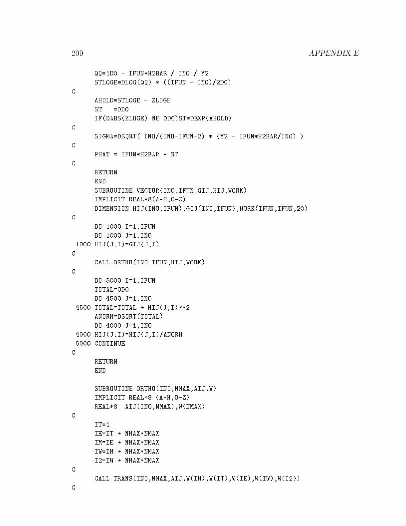
200 APPENDIX E
QQ=1D0 - IFUN*H2BAR / INO / Y2
STLOGE=DLOG(QQ) * ((IFUN - INO)/2D0)
C
AHOLD=STLOGE - ZLOGE
ST =0D0
IF(DABS(ZLOGE).NE.0D0)ST=DEXP(AHOLD)
C
SIGMA=DSQRT( INO/(INO-IFUN-2) * (Y2 - IFUN*H2BAR/INO) )
C
PHAT = IFUN*H2BAR * ST
C
RETURN
END
SUBROUTINE VECTOR(INO,IFUN,GIJ,HIJ,WORK)
IMPLICIT REAL*8(A-H,O-Z)
DIMENSION HIJ(INO,IFUN),GIJ(INO,IFUN),WORK(IFUN,IFUN,20)
C
DO 1000 I=1,IFUN
DO 1000 J=1,INO
1000 HIJ(J,I)=GIJ(J,I)
C
CALL ORTHO(INO,IFUN,HIJ,WORK)
C
DO 5000 I=1,IFUN
TOTAL=0D0
DO 4500 J=1,INO
4500 TOTAL=TOTAL + HIJ(J,I)**2
ANORM=DSQRT(TOTAL)
DO 4000 J=1,INO
4000 HIJ(J,I)=HIJ(J,I)/ANORM
5000 CONTINUE
C
RETURN
END
SUBROUTINE ORTHO(INO,NMAX,AIJ,W)
IMPLICIT REAL*8 (A-H,O-Z)
REAL*8 AIJ(INO,NMAX),W(NMAX)
C
IT=1
IE=IT + NMAX*NMAX
IM=IE + NMAX*NMAX
IW=IM + NMAX*NMAX
I2=IW + NMAX*NMAX
C
CALL TRANS(INO,NMAX,AIJ,W(IM),W(IT),W(IE),W(IW),W(I2))
C

Computing the \Student t-Distribution" 201
RETURN
END
SUBROUTINE TRANS
C(INO,NMAX,AIJ,METRIC,TRANSM,EIGV,WORK1,WORK2)
IMPLICIT REAL*8 (A-H,O-Z)
REAL*8 AIJ(INO,NMAX)
REAL*8 METRIC(NMAX,NMAX),EIGV(NMAX)
REAL*8 TRANSM(NMAX,NMAX),WORK1(NMAX),WORK2(NMAX)
DO 2000 I=1,NMAX
DO 2000 J=1,NMAX
TOTAL=0D0
DO 1000 K=1,INO
1000 TOTAL=TOTAL + AIJ(K,I)*AIJ(K,J)
METRIC(I,J)=TOTAL
2000 CONTINUE
C******************************************************************
C**** THIS CALL MUST BE REPLACED WITH THE CALL TO AN EIGENVALUE
C**** AND EIGENVECTOR ROUTINE
CALL EIGERS(NMAX,NMAX,METRIC,EIGV,1,TRANSM,WORK1,WORK2,IERR)
C**** NMAX IS THE ORDER OF THE MATRIX
C**** METRIC IS THE MATRIX FOR WHICH THE EIGENVALUES AND VECTORS
C**** ARE NEEDED
C**** EIGV MUST CONTAIN THE EIGENVALUES ON RETURN
C**** TRANSM MUST CONTAIN THE EIGENVECTORS ON RETURN
C**** WORK1 IS A WORK AREA USED BY MY ROUTINE AND MAY BE USED
C**** BY YOUR ROUTINE. ITS DIMENSION IS NMAX
C**** IN THIS ROUTINE. HOWEVER IT MAY BE DIMENSIONED
C**** AS LARGE AS NMAX*NMAX WITHOUT AFFECTING ANYTHING.
C**** WORK2 IS A SECOND WORK AREA AND IS OF DIMENSION NMAX
C**** IN THIS ROUTINE, IT MAY ALSO BE DIMENSIONED AS
C**** LARGE AS NMAX*NMAX WITHOUT AFFECTING ANYTHING.
C******************************************************************
DO 5120 K=1,INO
DO 3100 J=1,NMAX
3100 WORK1(J)=AIJ(K,J)
DO 5120 I=1,NMAX
TOTAL=0D0
DO 3512 J=1,NMAX
3512 TOTAL=TOTAL + TRANSM(J,I)*WORK1(J)
5120 AIJ(K,I)=TOTAL
RETURN
END

202 APPENDIX E

Bibliography
[1] Bretthorst G. L., (1987), Bayesian Spectrum Analysis and Parameter Estimation, Ph.D. thesis, Washington University, St. Louis, MO., available from Uni-versity Micro�lms Inc., Ann Arbor Mich.
[2] Robinson, E. A., (1982), \A Historical Perspective of Spectrum Estimation,"Proceedings of the IEEE, 70, pp. 855-906.
[3] Marple, S. L., (1987), Digital Spectral Analysis with Applications, Prentice-Hall,New Jersey.
[4] Laplace, P. S., (1812), Th�eorie Analytique des Probabilit�es, Paris, (2nd edition,1814; 3rd edition, 1820).
[5] Legendre, A. M., (1806), \Nouvelles M�ethods pour la D�etermination des Orbitsdes Com�etes," Paris.
[6] Gauss, K. F., (1963 reprint) Theory of the Motion of the Heavenly BodiesMoving About the Sun in Conic Sections, Dover Publications, Inc., New York.
[7] Cooley, J. W., P. A. Lewis, and P. D. Welch, (1967), \Historical Notes on theFast Fourier Transform," Proc. IEEE 55, pp. 1675-1677.
[8] Brigham, E., and R. E. Morrow, (1967), \The Fast Fourier Transform," Proc.
IEEE Spectrum, 4, pp. 63-70.
[9] Gentleman, W. M., (1968), \Matrix Multiplication and Fast Fourier Transfor-mations," Bell Syst. Tech. Journal, 17, pp. 1099-1103.
[10] Cooley, J. W., and J. W. Tukey, (1965), \An Algorithm for the Machine Calcula-tion of Complex Fourier Series," Mathematics of Computation, 19, pp. 297-301.
[11] Schuster, A., (1905), \The Periodogram and its Optical Analogy," Proceedings
of the Royal Society of London, 77, pp. 136.
[12] Jaynes, E. T. (1987), \Bayesian Spectrum and Chirp Analysis," inMaximumEntropy and Bayesian Spectral Analysis and Estimation Problems,C. Ray Smith, and G. J. Erickson, ed., D. Reidel, Dordrecht-Holland, pp. 1-37.
203
204 Bibliography
[13] Blackman, R. B., and J. W. Tukey, (1959), The Measurement of Power Spec-tra, Dover Publications, Inc., New York.
[14] Jaynes, E. T. (1983),Papers on Probability, Statistics and Statistical Physics,a reprint collection, D. Reidel, Dordrecht-Holland.
[15] Je�reys, H., (1939), Theory of Probability, Oxford University Press, London,(Later editions, 1948, 1961).
[16] Lord Rayleigh, (1879), Philosophical Magazine, 5, pp. 261.
[17] Tukey, J. W., several conversations with E. T. Jaynes, in the period 1980-1983.
[18] Waldmeier,M., (1961), The Sunspot Activity in the Years 1610-1960, Schulthes,Zurich.
[19] Nyquist, H., (1928), \Certain Topics in Telegraph Transmission Theory," Trans-actions AIEE, pp. 617.
[20] Nyquist, H., (1924), \Certain Factors A�ecting Telegraph Speed," Bell System
Technical Journal, 3, pp. 324.
[21] Hooke, R., and T. A. Jeeves, (1962), \Direct Search Solution of Numerical andStatistical Problems," J. Assoc. Comp. Mach., pp. 212-229.
[22] Wilde D. J., (1964), Optimum Seeking Methods, Prentice-Hall, Inc. EnglewoodCli�s, N. J.
[23] Zellner, A., (1980), in Bayesian Statistics, J. M. Bernardo, ed., Valencia Univer-sity Press, Valencia, Spain.
[24] Geisser, S., and J. Corn�eld, (1963), \Posterior Distribution for MultivariateNormal Parameters," Journal of the Royal Statistical Society, B25, pp. 368-376.
[25] Zellner, A., (1971), An Introduction to Bayesian Inference in Econometrics,John Wiley and Sons, New York. Second edition, (1987).
[26] Cox, R. T., (1961), The Algebra of Probable Inference, Johns-Hopkins Press,Baltimore, Md.
[27] Tribus, M., (1969), Rational Descriptions, Decisions and Designs, PergamonPress, Oxford.
[28] Schlaifer, R., (1959), Probability and Statistics for Business Decisions: anIntroduction to Managerial Economics Under Uncertainty, McGraw-Hill BookCompany, New York.
[29] Whittle, P., (1954), Appendix to H. Wold, Stationary Time Series, Almquist andWiksell, Stockholm, pp. 200-227.

Bibilography 205
[30] Shaw, D., (1976), Fourier Transform NMR Spectroscopy, Elsevier Scienti�c Pub.Co., New York.
[31] Ganem, J. W., and R. E. Norberg, (1987), Private Communication.
[32] Abragam, A., (1961), Principles of Nuclear Magnetism, Oxford Science Publica-tions, London.
[33] Beckett, R. J., (1979), The Temperature and Density Dependence of NuclearSpin-Spin Interactions in Hydrogen-Deuteride Gas and Fluid,Ph.D. thesis, Rutgers University, New Brunswick, New Jersey; available fromUniversity Micro�lms Inc., Ann Arbor Mich.
[34] Currie, R. G., (1985), Private Communication.
[35] Currie, R. G., and S. Hameed, (1986), \Climatically Induced Cyclic Variationsin United States Corn Yield and Possible Economic Implications," presented atthe Canadian Hydrology Symposium, Regina, Saskatchewan.
[36] Burg, John Parker, (1975), Maximum Entropy Spectral Analysis, Ph.D. Thesis,Stanford University; available from University Micro�lms Inc., Ann Arbor Mich.
[37] Cohen, T. J., and P. R. Lintz, (1974), \Long Term Periodicities in the SunspotCycle," Nature, 250, pp. 398.
[38] Sonett, C. P., (1982), \Sunspot Time Series: Spectrum From Square Law Mod-ulation of the Half Cycle," Geophysical Research Letters, 9 pp. 1313-1316.
[39] Bracewell, R. N,. (1986), \Simulating the Sunspot Cycle," Nature, 323, pp. 516.
[40] Jaynes, E. T., (1982), \On the Rationale of Maximum-Entropy Methods", Pro-ceedings of the IEEE, 70, pp. 939-952.
[41] Smith, W. H., and W. Schempp, (1987) private communication.
[42] Jaynes, E. T., (1976), \Con�dence Intervals vs. Bayesian Intervals," inFoundations of Probability Theory, Statistical Inference, and Statistical Theor-ies of Science, W. L. Harper and C. A. Hooker, editors, D. Reidel PublishingCo., pp. 252-253; reprinted in [14].
[43] Maxwell, J. C., (1860), \Illustration of the Dynamical Theory of Gases. Part I. Onthe Motion and Collision of Perfectly Elastic Spheres," Philosophical Magazine,
56.
[44] Herschel, J., (1850), Edinburgh Review, 92, pp. 14.
[45] Jaynes, E. T., (1968), \Prior Probabilities," IEEE Transactions on Systems Sci-
ence and Cybernetics, SSC-4, pp. 227-241; reprinted in [14].

206 Bibliography
[46] Jaynes, E. T., (1980), \Marginalization and Prior Probabilities," in Bayesian
Analysis in Econometrics and Statistics, A. Zellner, ed., North-Holland Publish-ing Company, Amsterdam; reprinted in [14].
[47] Laplace, P. S., (1814), A Philosophical Essay on Probabilities, Dover Publica-tions, Inc., New York, (1951, unabridged and unaltered reprint of Truscott andEmory translation).
Index
�t 22�l 33
� 15, 46, 47!2 61
! 50
f!g 2, 48Ak 33, 44Abragam, A. 118, 144absorption spectrum 132, 134accuracy estimates 20, 27, 50, 86, 98,
102, 100, 167aliasing 81amplitudes
nonorthonormal 13, 31orthonormal 33
applicationschirp analysis 158decay envelope extraction 144economic 134harmonically related frequencies 157multiple frequency estimation 151multiple measurements 161NMR 117, 144nonstationary frequency estimation
117orthogonal expansion 148
assumptions violating 74averaging data 163b 20
Bj 31, 44Bayes theorem 8, 16, 55, 57Beckett, R. J. 134Bessel inequality 35Blackman, R. B. 9, 23, 73Blackman-Tukey spectral estimate 72Bracewell, R. N. 151, 158
Brigham, E. 6Burg algorithm 135, 151Burg, J. P. 135, 151chirp 159C(!) 7Cohen, T. J. 148complete ignorance
choosing a prior 183of a location parameter 18, 185of a scale parameter 19, 187
Cooley, J. W. 6Corn�eld, J. 73cosine transform 7, 16Cox, R. T. 76Currie, R. G. 135D 9
di 13, 31d2 17
datacorn 135covariances 37di�raction 162economic 134NMR 118, 144
direct probability 9, 31discrete Fourier transform 7, 19, 89, 92,
105, 108, 110energy 25, 51expected
f!g Parameters 48amplitudes nonorthonormal 44amplitudes orthogonal 44variance 46
f(t) 13, 31Fisher, R. A. 74, 175frequency estimation
207
208 Index
common 120multiple 151one 13
gjk 32
Gauss, K. F. 5Gaussian 15
Gaussian approximation 20, 49, 88, 98Geisser, S. 73Gentleman, W. M. 6h2 35
hj 34
H 9
Hj(t) 33Hanning window 23, 73Herschel, J. 185Hooke, R. 50hyperparameter 59I 9
I(!) 7, 16, 71, 88, 97, 193improper prior
Je�reys 19uniform 18
intuitive picture 80Jaynes, E. T. 7, 13, 14, 16, 21, 23, 31,
50, 69, 98, 110, 151, 181, 185,186, 187, 195
Je�reys prior 19, 35, 46, 187Je�reys, H. 19, 55joint quasi-likelihood 18, 34Laplace, P. S. 5, 190least squares 2, 16Legendre, A. M. 5Lewis, A. 6likelihood 9
general model 31global 61one-frequency 13ratio 64
line power spectral density 114
Lintz, P. R. 148location parameter 18, 185m 31
marginal posterior probability de�nition10
Marple, S. L. 5, 8, 27maximum entropy 14maximum likelihood 2, 16Maxwell, J. C. 185mean-square
f!g 61di 17
hj 35
model 13adequacy 38Bracewell's 158chipped frequency 158decay envelope 144harmonically related frequencies 157intuitive picture 36multiple harmonic frequencies 108multiple nonstationary frequencies
115, 120one-frequency 13, 70with a chirp 159with a constant 137, 151with a Lorentzian decay 86, 122with a trend 137
orthonormal 33selection 55two-frequencies 94
Morrow, R. E. 6multiple frequency 108multiple measurements 120, 161noise 15, 78nonuniform sampling 81, 83Norberg, R. E. 118, 144nuisance function 137nuisance parameter 10, 18, 34, 146, 193Nyquist, H. 27Occam's razor 64orthnormality 33orthogonal expansion 64orthogonal projection 34orthonormal model
one-frequency 71one-frequency Lorentzian decay 87two-frequency 97
p(f!g) 25, 51

Index 209
pattern search routine 50periodogram 7, 18, 25, 72, 82, 92, 105,
110, 153posterior covariances
f!g 50fAg 45
posterior odds ratio 64, 107, 122posterior probability 9
approximate 40, 49fj 57, 61, 63general 35multiple measurements 135, 167multiple well separated frequencies
110of one-frequency with Lorentzian de-
cay 87of one-frequency 18, 71of the expansion order 149of two-frequencies 94, 98, 105of two-frequencies with trend 138of two well separated frequencies 95
power spectral density 25, 51, 72, 103,112
prior probability 9
!j 60fAg 59assigning 14, 183complete ignorance 183, 195Gaussian 185, 190improper priors as limits 189incorporation prior information 18,
34, 59, 190Je�reys 35, 187uniform 18, 34, 185, 189
prior see prior probabilityproduct rule 9, 120quadrature data 117R(!) 7, 16, 71, 97, 88, 193R� 62Rayleigh criterion 23relative probabilities 56, 63, 93residuals de�nition 5Robinson, E. A. 5S(!) 114
sampling distribution 9, 37scale parameter 19, 187Schempp, W. 162Schlaifer, R. 76Schuster, A. 7, 26second posterior moments 45Shaw, D. 117side lobes 26signal detection
multiple measurements 167one-frequency 21, 90
signal-to-noise 48sine transform 7, 16Smith, W. H. 162Sonett, C. P. 148, 151, 157, 158spectrum absorption 117stacking brute 163Student t-distribution 19, 35
computing 197one-frequency 71, 87multiple harmonic frequencies 109two-frequencies 94
su�cient statistic de�nition 7, 35, 110sum rule 10times discrete 13trend elimination 137Tribus, M. 76Tukey, J. W. 6, 9, 23, 73uniform prior 18, 34units conversion 21, 22variance 40, 47Waldmeier, M. 27weighted averages 190Welch, P. D. 6Whittle, P. 110Wilde, D. J. 50Wolf's relative sunspot numbers 27, 148y(t) de�nition 13Zellner, A. 55, 73, 76zero padding 19