áîÉêëáíó =çÑ=pçìíÜÉêå=`~ äáÑçêåá~ excel 2007...

© Mar

råAca

WhAs it Excelthesemanuany o

W

TABL

PROP

SORT

Sim

Co

FREE

Fre

Un

Ot

FILTE

Ap

Cle

Cr

Cr

Fil

Cr

FILTE

FILTE

Nu

Nu

rshall School of Bu

åáîÉêëáíóademic In

at is an Epertains to El provides an e tools includual. These daother type of

hat is an Exce

LE OF CONTEN

PER EXCEL DA

TING A DATAB

mple Sort ......

omplex Sort ...

EZE PANES .....

eeze Top Row

nfreeze Panes

ther Freeze Pa

ERING A DATA

pplying a Filte

earing a Crite

eating an “OR

eating an “OR

tering Multip

eating an “AN

ERING ‐ AND &

ERING ‐ WORK

umbers betwe

umbers Above

usiness ‐ USC

ó=çÑ=pçìínformatio

Excel Datxcel, a databaarray of toolse subtotals, fatabase featuinformation w

el Database?

NTS ...............

ATABASE CON

BASE ............

.....................

.....................

.....................

w (Row 1) .....

s ...................

anes Options

ABASE ..........

er ..................

eria or Remov

R” Condition

R” Condition

ple Columns –

ND” Condition

& OR CONDIT

KING WITH N

een Two Poin

e / Below Ave

Excel2007_D

íÜÉêå=`~on Servic

tabase? ase is a collecs you can usefiltering, sortiures can be uswhich is store

.....................

.....................

NSTRUCTION .

.....................

.....................

.....................

.....................

.....................

.....................

....................

.....................

.....................

ving the Filter

within the Sa

between Sep

– “AND” Cond

n within the S

TIONS ...........

NUMBER RAN

nts .................

erage ............

Databases.docx

~äáÑçêåá~es

ction related e to easily anaing, databasesed to analyzeed in a tabula

TABLE O

.....................

.....................

.....................

.....................

.....................

.....................

.....................

.....................

.....................

.....................

.....................

.....................

.....................

ame Column ..

parate Column

ditions ...........

Same Column

.....................

GES ..............

.....................

.....................

Wayn

~

data stored inalyze and mane functions ane survey dataar format.

OF CONTE

......................

......................

......................

......................

......................

......................

......................

......................

......................

......................

......................

......................

......................

......................

ns ..................

......................

n ....................

......................

......................

......................

......................

e Wilmeth

n tabular formnipulate yournd PivotTablesa, employee o

ENTS

.....................

.....................

.....................

.....................

.....................

.....................

.....................

.....................

.....................

.....................

.....................

.....................

.....................

.....................

.....................

.....................

.....................

.....................

.....................

.....................

.....................

mat. For datar data into uss which are cor student inf

.....................

.....................

.....................

.....................

.....................

.....................

.....................

.....................

.....................

.....................

.....................

.....................

.....................

.....................

.....................

.....................

.....................

.....................

.....................

.....................

.....................

2/6/09

Exce- Da

a stored in theful informatovered in a seformation, inv

.....................

.....................

.....................

.....................

.....................

.....................

.....................

.....................

.....................

.....................

.....................

.....................

.....................

.....................

.....................

.....................

.....................

.....................

.....................

.....................

.....................

of 68

el 2007tabases

is structure, tion. Some ofeparate ventory, or

.................... 1

.................... 1

.................... 5

.................... 8

.................... 8

.................... 8

.................... 9

.................... 9

.................... 9

.................... 9

.................. 10

.................. 10

.................. 10

.................. 11

.................. 11

.................. 11

.................. 11

.................. 11

.................. 12

.................. 12

.................. 13

f

1

1

5

8

8

8

9

9

9

9

0

0

0

1

1

1

1

1

2

2

3

© Marshall School of Business ‐ USC Excel2007_Databases.docx Wayne Wilmeth 2/6/09 of 68

Displaying the X Highest (or Lowest) Numbers in a Field (Column) ................................................................................. 13

Displaying a Given Percent of the Highest (or Lowest) Values in a Field (Column) .......................................................... 14

FILTERING – WORKING WITH DATE RANGES ........................................................................................................................ 15

FILTERING – WORKING WITH TEXT FILTERS .......................................................................................................................... 16

Display Only Records that Contain Blanks ........................................................................................................................ 17

Hide Records that Contain Blanks ..................................................................................................................................... 17

Using Wildcards for Special Searches ............................................................................................................................... 17

Using “AND” & “OR” with a Single Text Field ................................................................................................................... 18

FILTERING ‐ FILTER BASED ON FORMATTING COLOR ........................................................................................................... 19

Part 1: Setting the Conditional Formatting .................................................................................................................. 19

Part 2: Filtering (Or Sort) Based on Color ..................................................................................................................... 21

Clearing the “Profit” Filter ................................................................................................................................................ 21

Clearing Conditional Formatting ....................................................................................................................................... 21

THE ADVANCED FILTER AND DATABASE FUNCTIONS ........................................................................................................... 22

Setting‐Up the Criteria Area for Database Functions ....................................................................................................... 22

THE DATABASE FUNCTIONS .................................................................................................................................................. 23

DSum() Example ................................................................................................................................................................ 23

Dsum() Example Continued: Using a Simple Criteria .................................................................................................... 23

Dsum() Example Continued: Using an “OR” between Separate Columns .................................................................... 24

Dsum() Example Continued: Using an “AND” between Separate Columns ................................................................. 24

Dsum() Example Continued: Using an “OR” within the Same Column ......................................................................... 24

Dsum() Example Continued – Number & Date Ranges ..................................................................................................... 25

Dsum() Example Continued – Using “AND” with Number & Date Ranges ....................................................................... 25

USING THE ADVANCED FILTER TO FILTER IN PLACE OR EXTRACT RECORDS ........................................................................ 26

Filter a List in Place ............................................................................................................................................................ 26

Criteria Changes ................................................................................................................................................................ 26

Clear the Advanced Filter .................................................................................................................................................. 26

Copy Matching Records to another Location ................................................................................................................... 27

USING RANGE NAMES WITH DATABASES ............................................................................................................................. 28

SAVING DATABASE FUNCTION RESULTS BY USING MULTIPLE CRITERIA AREAS .................................................................. 29

WORKING WITH DUPLICATE RECORDS ................................................................................................................................. 30

Identifying Duplicate Records ........................................................................................................................................... 30

Delete Duplicate Records .................................................................................................................................................. 31

VLOOKUP() ............................................................................................................................................................................ 32

Simple Vlookup Example ................................................................................................................................................... 32

Vlookup Example – Compare Two Different Lists (Exact Text Match) .............................................................................. 33

Vlookup() Example – Return a Value in a Range (Approximate Numeric Match) ............................................................ 35

Vlookup() Example – Numeric Range to Assign Grades .................................................................................................... 37


GROUPING COLUMNS ........................................................................................................................................................... 38

GROUPING ROWS AND AUTO OUTLINE ................................................................................................................................ 39

Grouping Rows .................................................................................................................................................................. 39

Auto Outline ...................................................................................................................................................................... 39

SUBTOTALS ............................................................................................................................................................................ 40

Removing the Subtotals .................................................................................................................................................... 40

CONVERT YOU DATABASE TO A TABLE ................................................................................................................................. 41

Converting a Database into a Table .................................................................................................................................. 41

Table Styles and Style Options .......................................................................................................................................... 42

Tables ‐ Adjusting the Table’s Range ................................................................................................................................ 43

Table Tools ........................................................................................................................................................................ 43

Tables ‐ Using the Subtotal() Function Outside of the Table ............................................................................................ 44

Example: Using Subtotal() on Another Sheet ............................................................................................................... 44

Combining Tables to Get Grand Totals ............................................................................................................................. 44

DATA VALIDATION ................................................................................................................................................................ 45

General Overview ............................................................................................................................................................. 45

Extending the Data Validation Range to New Rows ......................................................................................................... 46

Clearing Validation ............................................................................................................................................................ 46

Applying Multiple Validation Rules to the Same Cells ...................................................................................................... 46

Example: Limit Data Entry to List .................................................................................................................................. 47

Example: Text (or Number) Length ............................................................................................................................... 48

Example: Whole Numbers Only Range (10, 1, 3, etc.) .................................................................................................. 48

Example: Decimal Numbers Range (i.e. 10.5) ............................................................................................................... 48

Date Ranges ...................................................................................................................................................................... 49

CUSTOM DATA VALIDATION FORMULAS .............................................................................................................................. 50

Custom Validation Example: Down Payment 20% Percent of Price ............................................................................. 50

Custom Validation Example: Data Entry Depends upon another Cell ........................................................................... 51

“OR” Example – Control the First Four Characters Only ................................................................................................... 52

“AND” Example – Control where Dashes Appear and Total Length ................................................................................. 53

Prevent Duplicate Entries in a Column ............................................................................................................................. 54

CLEANING UP DATA ISSUES .................................................................................................................................................. 55

Format Numbers to Include Leading Zeros ....................................................................................................................... 55

Format ID Numbers with Dashes ...................................................................................................................................... 56

Remove Hard Coded Dashes – Find and Replace ............................................................................................................. 56

Store Numbers as Text to include Leading Zeros .............................................................................................................. 57

Remove any Leading or Training Spaces – Trim() ............................................................................................................. 58

Converting Formulas to their Values ................................................................................................................................ 58

Concatenation – Display the Contents of Many Cells in One Cell .................................................................................... 59


Break a Cell’s Content Into Multiple Cells (Parse) ............................................................................................................ 60

Transpose – Swap Columns & Rows ................................................................................................................................. 61

WORKING WITH EXTERNAL DATA ......................................................................................................................................... 62

Linking to an Access Database .......................................................................................................................................... 62

Refresh the Data ............................................................................................................................................................... 63

Break the Link to Access.................................................................................................................................................... 63

Linking to Tables from the Web ........................................................................................................................................ 64

Linking to an SQL Server Database ................................................................................................................................... 65

APPENDIX ‐ EXCEL DATABASES VS. ACCESS DATABASES ...................................................................................................... 67

The Difference between Excel and Access Databases ...................................................................................................... 67

When to use Excel Databases and when to use Access Databases .................................................................................. 67


DIVIDE DATA INTO SEPARATE COLUMNS The attributes of a particular item, person, etc., should be separated into different columns. This allows you to filter, sort, subtotal, etc., on each separate column. You should also use column headings.

PLACE RELATED DATA IN THE SAME ROW Data which pertains to the same item, person, etc., should be in the same row. For example, all the data in the same row as Fried Green Tomatoes pertains just to that movie. It was produced by Universal, has an R rating, is a Drama, made $50,879,690, and was made on 12/27/1996.

Definition: Cell = “Field” In a database, each cell is called a “Field” and the column title is known as the “Field Name”. For example, the Rating field contains the ratings.

Definition: Row = “Record” A single row of information is known as a “Record”. A record consists of the attributes of a particular item, person, etc.

PROPER EXCEL DATABASE CONSTRUCTION These next few pages cover how to properly construct an Excel database. The database tools available in Excel depend upon your database having a very specific structure.

MORE ON DIVIDING YOUR DATA INTO SEPARATE COLUMNS As covered above, data should be divided into separate columns. The degree of separation typically depends upon what you wish to do with the data. Filtering, sorting, mathematical operations, pivot tables, mail merges, all require the data to be isolated within its field.

Limiting Construction In the table to the left, the data is divided into separate columns, but not enough. You are not able to sort or filter by last name, city, state, or zip code because they are buried within the data of the field.

Versatile Construction The image to the left correctly shows each item in its own field. Note that if you were in real‐estate, you might even consider separating house number from street name.


NO COMPLETELY BLANK ROWS OR COLUMNS Your database must not contain any completely blank columns or rows within the database area. When sorting or using most other database tools, Excel assumes that any adjacent data is part of the database and should be included in any sorting, filtering, subtotals, etc. If there are any gaps between columns or rows, the data on the other side of the gap will not be included. This can be disastrous when sorting because you will lose your record integrity. For example, in the image below there is a blank column in the middle of the database. If you were to sort by “Movie”, the data the Production Co and Movie column would sort alphabetically but the data in Rating, Category, Profit, and Year would remain in its current position which would result in a loss of record integrity. Each movie would no longer be in correct row as its Rating, Category, Profit, or Year.

No completely blank rows or columns!

Random Blanks are Fine as Long as at Least one Field in the Row Contains Data As long as at least one field in a row contains data, Excel will find the data below the row.

Blanks in a Column are Fine if you have a Field Heading You can have a blank column if your column has a field heading. This will not adversely affect your database.


No Vertical Calculations within the Database While databases may contain calculated fields between columns, the calculations should not include cell addresses in a row that is different from the row the formula is in. As soon as you sort, your data and the formulas would rearrange within the column and the formulas would return the wrong answer. For example, in the image shown to the right there are subtotals for each quarter. As soon as the database is sorted by any column, the formulas would become meaningless. Note that Excel does provide a subtotal database function that can instantly create subtotals for you!

Horizontal Calculations are Fine Calculations that use data cell addresses in the same row as the formula cell are fine. For example, in the image to the right, Cost Per Item was computed by dividing Cost Per Case by Items Per Case. Because all cells involved are in the same row, problems will not result when you sort or use other Excel database features.


SORTING A DATABASE Sorting alphabetizes your database based on a specific column or columns. For example, you wish to alphabetize by movie name or you want the highest grossing movies at the top of the list. You can sort in either ascending (A‐Z) or descending (Z‐A) order.

Simple Sort To sort on just one column, follow the steps below. Do not highlight first! As long as your database has no completely blank rows or columns, all columns and rows will participate in the sort. If you did highlight first, only the highlighted area would sort which would lead to the loss of data integrity.

1. Click the “Movies” sheet. 2. Click anywhere in the column you wish to sort by. (For example, to sort by movie, click on any movie.) 3. Click the “Data” tab. 4. Click either the Ascending or Descending sort buttons.

Sorts text from A‐Z, dates from oldest to newest, and numbers from smallest to largest.

Sorts text from Z‐A, dates from latest to oldest, and numbers from largest to smallest.

Complex Sort To sort multiple columns (i.e. first by “Production Company”, then by “Movie”) you must use the “SORT” button. 1. Click on any single cell within the database. (Again, do not highlight multiple cells.) 2. Click the “Data” tab. 3. Click the “Sort” button. 4. Follow steps a‐e below and click “OK”.

b. Sort on For numbers or letters,

set this to “Value”.

c. Order Set to ascending (A to Z)

or descending (Z to A).

a. Sort By Select the primary

field you wish to alphabetize by.

d. Check this if your database has column headings.

e. Click “Add Level” to get another row for a sub‐sort and fill out the new row.


FREEZE PANES This feature is very useful when you have long or wide database because it allows you to scroll through the data while still being able to see the column (or row) headings.

Freeze Top Row (Row 1) In this example, we will freeze the names of the column titles. 1. Click the “Movies” sheet. 2. Click the “View” tab. 3. Click the “Freeze Panes” drop down and select “Freeze Top Row”. (This always freezes row 1.) If you scroll down the database, you will see that the column titles are frozen into place.

Unfreeze Panes To unfreeze any froze panes: 1. Click the “View” tab. 2. Click “Freeze Panes”. 3. Click “Unfreeze Panes”.

Other Freeze Panes Options The illustration below covers some other useful freeze panes options.

Freeze Panes – This freeze all rows above and all columns to the left of your cursor. It is useful when you database does not start in cell A1. Freeze Top Row – This always freezes row 1 or the first non hidden row. Freeze First Column – This always freezes column A or the first non hidden column.


FILTERING A DATABASE Filtering allows you to hide records (rows) based on criteria you select from a drop down list. Filtering provides the following abilities:

• Hide records based on a text, numbers, and dates using specific matches, partial matches, and ranges. • Create “AND” conditions between separate columns. (i.e. Any G rated Paramount movie.) • Create “OR” conditions within the same column. (i.e. Any G or any PG movies.) • Filtering cannot create OR conditions between separate columns. (i.e. Any G movie or any Disney Movie.)

(See the Advanced Filtering for “OR” conditions between columns.)

Applying a Filter 1. Click anywhere within the database area. 2. Click the “Data” tab. 3. Click the “Filter” button. (Drop down arrows should appear next to each field heading.) 4. Click the drop down arrow for the column which contains data you wish to filter by. 5. Uncheck the items you wish to hide and click “OK”.

Clearing a Criteria or Removing the Filter When a filter is currently in effect, the row numbers will turn blue and the drop down arrows for any columns taking part in the filter will have small filters on them. To Remove a Specific Condition: • One‐by‐one, click all drop down arrows with filters on them and click the

“Clear Filters From…” option.

To Remove all Conditions and the Filter Arrows: • Click the “Filter” button located on the “Data” tab.

Sorting the Column If desired, you can also use the options in this area to sort the database by the column.

Clear the Filter Clears the selected column’s filter. Filter by Color Hides all but the selected text color. Text Filters / Number Filters Allows custom filtering and filtering using ranges. See the next page for more on this option. Data Specific Filtering Uncheck a box to hide records containing the criteria; check a box to display records containing the criteria. Click “Select All” to quickly check or uncheck all


Creating an “OR” Condition within the Same Column Whenever you check multiple criteria in the same column, you are creating an “OR” condition. For example, if you where to check both “G” and “PG” in a column called Rating, you are essentially telling Excel: “Show me only G or PG rated movies.” It is important to realize that this is not an “AND” condition. Using “AND” would be like saying that a single cell has both a “G” rating and a “PG” rating which no cell should have it you designed your database correctly.

Creating an “OR” Condition between Separate Columns An example of this would be: “Display only Paramount movies OR G rated movies.” This is different from an “AND” condition because unlike “AND”, “OR” specifies that for a movie to display, it doesn’t have to have be both by Paramount and be G rated, it just needs to meet one or the other. “OR” between separate columns is not possible using the “Filter” button. See the section on using the “Advanced Filter” for creating an “OR” condition between separate columns.

Filtering Multiple Columns – “AND” Conditions Whenever you set a criteria using more than one column in the same database, you have created an “AND” condition. For example, if you select “PG” in the “Rating” column and “Comedy” in the “Category” column then you are in effect telling Excel the following: Only display movies whose Rating is PG AND whose Category is Comedy. A particular movie must have a PG rating and it must also be a comedy to be displayed.

Creating an “AND” Condition within the Same Column For the most part, an “AND” condition within the same column only works with date or number ranges. For example: “Show movies whose profit was greater than 100,000,000 AND less than 200,000,000. For Text columns, unless you are using “begins with in combinations with ends with”, an “AND” condition would produce nothing. For example, there is no movie that has both a G rating and an R rating. Number ranges are covered later.

FILTERING AND & OR CONDITIONS This section covers what actions create an “AND” condition and what actions create an “OR” condition. When using “AND”, all criteria must be met for a row to be displayed. When using “OR”, only one of the criteria must be met for the row to be displayed. Using the Filter, “AND” conditions are only possible between different columns and within the same column using number or date ranges. “OR” conditions are only possible within the same column unless you use the advanced filter.


FILTERING WORKING WITH NUMBER RANGES

This section covers how to return a range of numbers. For example, all movies that made between 200 million and 300 million or movies that made above average. The range features are available under the “Number Filters” Note that except for Top 10, Above Average, and Below Average, all of the options under the Number Filters menu take you to the same window, they just fill out the form slightly differently in each case.

Numbers between Two Points In this example, we will list only movies which made between 200 million and 300 million dollars profit. Note that “between” is inclusive of the 200 and 300 million.

1. Click the drop down for “Profit”. 2. Click “Number Filters”. 3. Click “Between”. Note that the left side of the screen is already filled out for you to reflect a “between” range. If desired, you could change the left side.

4. In the criteria for Is greater than or equal to, type: 200000000

5. In the criteria for Is less than or equal to, type: 300000000

6. Click “OK”.

Note that this used the “AND” operator between the high and the low range. When you are searching for numbers or dates between two points, you will always use the “AND” operator. You would only use “OR” with number or date ranges if you were looking for the outside extremes. For example, movies that made less than 50 million OR greater than 300 million.


This feature will automatically compute the average of all numbers in a field (column) and then display any records above or below the average. Note that profit cells containing blanks are not included in Excel’s computations to get the average and Excel does not display what the average is. 1. Click the drop down for a number field. (Profit in this example.) 2. Click “Number Filters”. 3. Click “Above Average” or “Below Average”. Excel should now be displaying only those records whose profit is either above or below the average depending upon which option you selected.

Numbers Above / Below Average

Displaying the X Highest (or Lowest) Numbers in a Field (Column) This feature allows you to display only a specified number of highest or lowest scores for a field. For example, in a table of student scores you would like to display just the students with the highest three scores. 1. Click the drop down for your number field. (Score in this example.) 2. Click the “Number Filters” option. 3. Click “Top 10…” 4. Make the settings shown then click “OK”.

This can be set to either “Top” or “Bottom”.

This can be set to either “Items” or “Percent”.

Type a value here or use the arrows to select one.

The database now only displays records for the three highest scoring students.


Displaying a Given Percent of the Highest (or Lowest) Values in a Field This feature allows you to display only records that contain data within a top (or bottom) percentage. For example, you wish to only display scores in the top 25 percentile. 1. Click the drop down for your number field. (Score in this example.) 2. Click the “Number Filters” option. 3. Click “Top 10…” 4. Make the settings shown below then click “OK”.

The database now only displays records for the scores in the top 25 percent. This can be a little tricky to interpret. First, you might want to determine where the 25 percent breakpoint for the 10 records would be. 25% of 10 records is 2.5 records (.25*10). This means that you should display just the top 2.5 records but because Excel cannot display half a record, it displays just the top 2 records.


FILTERING – WORKING WITH DATE RANGES Date ranges work pretty much the same way as number ranges with just a few more options.

Click to Select/Deselect The first difference you might notice is on the list, only years are listed. If you would like to only view specific months or days in a year, simply click the year’s and month’s expand button so you can uncheck specific dates. Instant Filters Another difference is the type of Date Filters. As you can see from the image to the left, there are many presets which filter for you using your computer’s internal date. Tomorrow, Today, Yesterday, Next Week, etc., all use your computer’s clock to filter records. There is no need to input any other data. All Dates in the Period This displays another set of instant filters that also require no other input on your part.

Custom Filters Any of the options followed by three dots (…) will bring up the image shown to the left. This requires that you set the criteria yourself. You can either type dates in or select them from the calendar icon.


FILTERING – WORKING WITH TEXT FILTERS

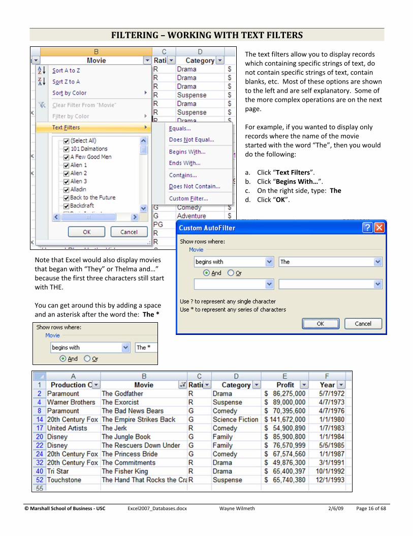
The text filters allow you to display records which containing specific strings of text, do not contain specific strings of text, contain blanks, etc. Most of these options are shown to the left and are self explanatory. Some of the more complex operations are on the next page. For example, if you wanted to display only records where the name of the movie started with the word “The”, then you would do the following: a. Click “Text Filters”. b. Click “Begins With…”. c. On the right side, type: The d. Click “OK”.

Note that Excel would also display movies that began with “They” or Thelma and…” because the first three characters still start with THE. You can get around this by adding a space and an asterisk after the word the: The *


Display Only Blank Records To display only records that contain a blank in a specific field, follow the steps below. 1. Click the drop down arrow for the column you suspect contains blank

fields. 2. Click “Select All” to uncheck all criteria. 3. Check “(Blanks)”. 4. Click “OK”. Note that if the column contains no blacks then the “(Blanks)” options will not be listed.

Hide Blank Records To hide any record that contains a blank in a specific field, follow the steps below.

1. Click the drop down arrow for the column you suspect contains blank fields.

2. Click “Text Filters” then “Contains”. 3. Type an asterisk ( * ) in the criteria box. 5. Click “OK”.

Note: The asterisk is a wild card which stands in for multiple characters. You are basically saying, “Only show records which contain something.”

Using Wildcards for Special Searches Most of the time, the instant filters (Begins with…, Ends with.., etc) will suffice for text searches; however, there are times when you will need to use “wildcards”. Wildcards cards are symbols which can stand it for any character and Excel has two available: * The asterisk can stand in for any number of characters. For example, if you wanted to display only records

that end in “ing”, you would type: *ing You are telling Excel, “I don’t care what comes first but it must end in “ing”.”

? The question mark can stand in for only a single character. For example, if you wanted to find anyone named Smith or Smyth, you would type: Sm?th Note that Excel would not return “Smooth” because there is an extra character. Only Sm??th would return “Smooth” (but would not return “Smith” or “Smyth”).


Using “AND” & “OR” with a Single Text Field “OR” is often used in text fields; for example, whenever you check multiple boxes on the drop down, you are creating an “OR” condition. There are few times you will use an “AND” condition within a single text field. Examples of using the Custom AutoFilter with an “AND” and an “OR” are shown below.

Custom “OR” Example In this example, we wish to see any company that ends in “Inc.” or “LTD.”. 1. Click “Text Filters”. 2. Click “Custom Filters…”. 3. Make the settings shown to the left. 4. Click “OK. Note that we used “OR” between the two conditions. “AND” would have returned nothing because there is no single company name that ends in both Inc. and Ltd.

Custom “AND” Example “AND” can only be used within a single text field when the criteria is non inclusive. For example: We wish to only view Movies that begin with “The” and end with “Ing”. Because a single movie can both begin with “The” and end with “ing”, you should use “AND”. 1. Click “Text Filters”. 2. Click “Custom Filters…”. 3. Make the settings shown to the left. 4. Click “OK.

Finding a Range of Initial Letters In this example, we wish to only display movies that start with the initial letters of J‐P. The only range operators you can use with letters are: “is greater than” and “is less than”. Therefore, we must look for movies greater than “I” and less than “Q”. 1. Click “Text Filters”. 2. Click “Custom Filters…”. 3. Make the settings shown to the left. 4. Click “OK. Do not use Wildcards with letter ranges!


FILTERING FILTER BASED ON FORMATTING COLOR If you have applied a color formatting to a cell either manually or through Conditional Formatting, you can filter your database based on the formatting. Excel can filter using either text color or cell fill color. In this example we will first format our cells using conditional formatting and then filter based on color.

Part 1: Setting the Conditional Formatting One of the benefits of filtering based on formatting is it provides a method of saving your criteria through the use of color. In this example, we will use conditional formatting as follows: Profit less than 100,000,000: Pink Background Profit between 100,000,000 and 200,000,000: Yellow Background Profit Greater than 200,000,000: Green Background Note that “Between” is inclusive and “Greater Than” is exclusive.

1. Click the column letter above “Profit” to highlight the entire column. 2. Click the “Home” tab. 3. Click the “Conditional Formatting” button.

We can do this either through “New Rule and then “Format Cells that Contain” or by using the quick select options. Because the quick select buttons are easier to use, we will opt for that method. Profit less than 100M 4. Click “Highlight Cells Rules”. 5. Click “Less Than…”

6. In the left box, type: 100000000 7. In the right box, click the down

arrow and select “Custom Format…”.

Clearing a Rule To clear, manage, or create a new rule, use these options.


8. Click the “Fill” tab. 9. Click a fill color (pink in this example). 10. Click “OK” then “OK” again.

Profit Greater than 200M 20. With the column still highlighted, click the “Conditional Formatting” button again. 21. Click “Highlight Cells Rules”. 22. Click “Greater Than”. 23. Type 200000000 in the lower limit box. 24. Click the drop down arrow and select “Custom Format”. 25. Click the “Fill” tab. 26. Click the color green. 27. Click “OK” then “OK” again.

12. Click “Highlight Cells Rules”. 13. Click “Between…”. 14. In the lower limit box, type: 100000000 15. In the upper limit box, type: 200000000 16. Click the drop down and select “Custom Format”. 17. Click the “Fill” tab. 18. Click the color yellow. 19. Click “OK” then click “OK” again.

Profit Between 100M and 200M 11. With the column still highlighted, click the “Conditional Formatting”

button again.


Part 2: Filtering (Or Sort) Based on Color Now that we have formatted our cells with color, we can use the Auto Filter to only display cells of a specific color. 1. Click the drop down for “Profit”. 2. Click “Filter by Color” and then select a color.

Clearing the “Profit” Filter To clear a column’s filter: 1. Click the columns filter drop down arrow. 2. Click “Clear Filter from “Profit”.

Clearing Conditional Formatting To remove any colors you have applied to your database using conditional formatting, follow the steps below. 1. Click the “Home” tab. 2. Click the “Conditional Formatting” button. 3. Click “Clear Rules”.

• To remove the colors anywhere in the sheet, click “Clear Rules for Entire Sheet”.

• To remove the colors just for cells you are highlighting, click “Clear Rules from Selected Cells”.


THE ADVANCED FILTER AND DATABASE FUNCTIONS The Advanced Filter is somewhat more complicated than using Auto‐filter but it does provide some features that the Auto‐filter button does not. You would use the Advanced Filter when you with to do the following:

• Use Database Functions – Excel has several Database functions such DSum(), Daverage(), DCount(), etc, that perform their computations only on records which meet your criteria. As soon as you change your criteria, the functions automatically update.

• Perform “OR” Conditions Between Columns ‐ You cannot perform an “OR” condition between columns using the Auto‐filter ‐ you must use the Advanced Filter for this. An example of an “OR” condition between separate columns would be: “Show movies produced by Disney OR G rated movies.”

• Extracting Data – You wish to extract the matching data to a different location.

Setting-Up the Criteria Area for Database Functions When using either the Advanced‐filter or Database Functions, you will need to add a “Criteria” area to your database where you will be typing your search parameters directly into the criteria area.

1. Copy your all of your field headings for the database to another location. • I’ve placed them above the current database but they can be on a separate sheet as well. • Make sure you leave several blank rows below the new headings so you will have room to type your

criteria. Each blank row can be used as an “or” condition.

The advanced filter utilized two distinct areas: The Criteria Area and the Database Area. If you will be extracting, you will also need an Extraction area. Criteria Area – This is the top range shown above (A1:F4) and must included your duplicate column headings and

a few rows for any “OR” conditions. You will be typing your conditions in this area. Database Area ‐ This is the partially shown area above (A6:F54) and must include your entire database including the

column headings. Extraction Area ‐ If you will be copying data to another location, you will need a third copy of your column headings

somewhere else. This technique will be cover later.

Criteria Area

Database Area


1. Click in a cell off to the side of your database (J2 for example). 2. Type the following: =Dsum(A6:F54,"Profit",A1:F4) and press enter. Excel should return the total profit of all movies.

THE DATABASE FUNCTIONS AND THE ADVANCED FILTER Excel has several database functions. The most commonly used database functions are: Dcount(), Dsum(), and Daverage(). They are designed to work with your database and criteria area to produce their solutions.

DSum() Example We wish to sum up the total profit for all movies. Because we wish to include all movies, we will not be typing anything in the criteria area. Syntax: =Dsum(Database Range, “Column Name”, Criteria Range)

This is includes the column headings and all of the data in your database. In this example, it is: A6:F54

This is the name of the column you wish to sum in quotes. In this example: “Profit”.

This is the area where you will be typing your conditions. In this example, A1:F4.

Dsum() Example Continued: Using a Simple Criteria In this example, we wish to sum the profit of just Disney movies. It will require us to type in the criteria area.

1. Type the word Disney in cells A2, A3, & A4 as shown below. Note that as soon as you fill in the 4th row A4, the Dsum() function will update to sum only Disney movies.

Why Disney three times? As you may recall, each row we specify in our criteria area acts as an “OR” condition and our criteria area includes three blank rows. A blank row tells Excel it can return anything. If we had typed Disney only once, we would be saying: Sum Disney or anything, or anything and you would get the grand total for all movies. By typing Disney three times we are saying: Sum Disney or Disney or Disney. Note that rather than repeating Disney three times, you can also specify a production company that does not exist. For example, you could type Disney in A2 and a Z in A3 & A4. You would be saying: Sum Disney or Z or Z.

Note that the database does not update. Only the function updates.


Dsum() Example Continued: Using an “OR” between Separate Columns One thing the Advanced‐filter can do that the Auto‐filter cannot is to perform an “OR” condition between separate columns. In this example, we wish to sum movies which are either rated “R” or are categorized as “Suspense”.

1. Type an R in C2. 2. Type the word Suspense in D3. 3. Type a Z in C4. (We know there are no Z rated movies). Dsum should now update to sum only Suspense or R rated movies.

Dsum() Example Continued: Using an “AND” between Separate Columns If you type a criteria in different columns but in the same row, you have created an “AND” condition. In this example, we wish to sum R rated Dramas.

1. Type an R in C2. 2. Type the word Drama in D2. 3. Type a Z in D3 and D4. (The Zs can actually go in any column of row 3 & 4. We use Z because there is no Z category). Dsum should now update to sum only Dramas rated R.

Dsum() Example Continued: Using an “OR” within the Same Column In this example, we wish to sum the profit for only G & PG movies.

1. Type a G in C2. 2. Type a PG C3. 3. Type a Z in C4. (We know there are no Z rated movies). Dsum should now update to sum only G & PG rated movies.


Dsum() Example Continued – Number & Date Ranges You can use the following comparison operators when working with numbers or date:

Greater than: > Less than: < Greater than or Equal to: >= Less than or Equal to: <= Equal to: = Note Equal to: <>

The example below shows the criteria you would use to sum only movies whose profit is greater than 500 million. Again, the Zs in rows 3 & 4 are there because the extra rows act as OR conditions and there are no Z rated movies.

1. In the criteria area, repeat the column heading involved to the far right of the criteria area. In this example, we have repeated the work “Year” because it is the column involved.

2. Type your criteria using both columns as shown. (As you may recall, items in separate columns but in the same row act as an “AND” condition.)

Dsum() Example Continued – Using “AND” with Number & Date Ranges To create number or date rate between two points, for example >=1/1/1985 and <=12/31/1985, you will need to repeat the column heading involved in the criteria row and extend your criteria section to include the repeated column heading.

3. In the Dsum() formula, extend the criteria area to include the new column. (In this example, we changed it from A1:F4 to A1:G4).


USING THE ADVANCED FILTER TO FILTER IN PLACE OR EXTRACT RECORDS These features of the Advanced‐filter allow you to filter the list in place, extract filtered records to a different location, or extract only unique filtered records. Their usefulness has been somewhat usurped by the Auto‐filter; however, this still provides the only method to filter using an “OR” between separate columns and its ability to extract only unique records is also useful.

Filter a List in Place Use this feature to display only records which match the conditions specified in the criteria area. In this example, we wish to view only movies rated G or whose category is Comedy. 1. See page 22 for instructions on setting up the criteria area of the advanced filter. 2. Set‐up the criteria as shown below. (G is repeated in C4 because row 4 is an “OR” row.)

3. Click the “Data” tab and then the “Advanced” button. 4. Check “Filter the list, in‐place”. 5. Set the List Range to: A6:F59 (This is the database range including titles. The $ are optional.) 6. Set the Criteria Range to: A1:F4 (This is where you type your criteria. The $ are optional.) 7. Click “OK”. Any unmatched records should be hidden.

Criteria Changes Although the database functions will instantly update when you change the conditions in the criteria area, the filtered list will not. To update the filtered list, simply repeat steps 3 & 7 above.

Clear the Advanced Filter To view all of your records, do the following: 1. Click the “Data” tab and then click “Clear”.


Copy Matching Records to another Location Rather than filtering a list in place, “Extract Records” will copy only the matching records to a new location. When extracting records, you must copy the table’s column headings to location where you wish to extract the records to. In this example, we will copy them to A100. 1. Highlight your database’s column headings. 2. Press CONTROL + C to copy. 3. Click in cell A100 and press CONTROL + V to paste.

4. Click the “Data” tab and then the “Advanced” button. 5. Check “Copy to another location”. 6. Set the List Range to: A6:F59 (This is the database range including titles. The $ are optional.) 7. Set the Criteria Range to: A1:F4 (This is where you type your criteria. The $ are optional.) 8. Set Copy to to: A100:F100 (This is the range of your third set of column headings. Again, the $ are

optional.) 9. If desired, check “Unique records only”. When checked, only one copy

of any duplicate records will be copied. 10. Click “OK”. If scroll to A100, you will see only those records which match your criteria.


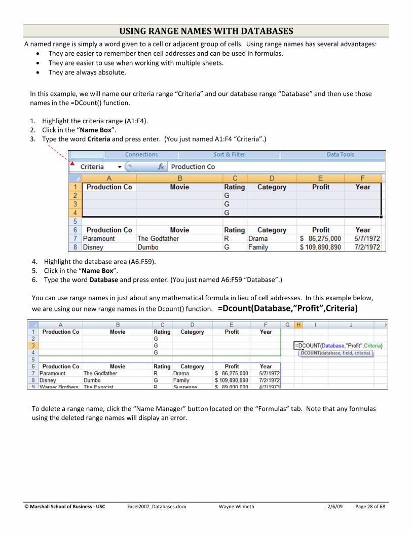
USING RANGE NAMES WITH DATABASES A named range is simply a word given to a cell or adjacent group of cells. Using range names has several advantages:

• They are easier to remember then cell addresses and can be used in formulas. • They are easier to use when working with multiple sheets. • They are always absolute.

In this example, we will name our criteria range “Criteria” and our database range “Database” and then use those names in the =DCount() function. 1. Highlight the criteria range (A1:F4). 2. Click in the “Name Box”. 3. Type the word Criteria and press enter. (You just named A1:F4 “Criteria”.)

4. Highlight the database area (A6:F59). 5. Click in the “Name Box”. 6. Type the word Database and press enter. (You just named A6:F59 “Database”.) You can use range names in just about any mathematical formula in lieu of cell addresses. In this example below,

we are using our new range names in the Dcount() function. =Dcount(Database,”Profit”,Criteria)

To delete a range name, click the “Name Manager” button located on the “Formulas” tab. Note that any formulas using the deleted range names will display an error.


SAVING DATABASE FUNCTION RESULTS BY USING MULTIPLE CRITERIA AREAS There is no reason why you cannot create multiple criteria areas for the same database. This is desirable when you have several different questions you wish to answer and you don’t want to erase the previous condition to create the next one. Each of the four criteria areas below query the same database.

The formulas for each of the results above are shown here. Note that the only thing (aside from the function type) that changes is the range of the criteria area. Each of the functions refer to the same database (A6:A59) which we range named “Database” and the same column of “Profit”.


WORKING WITH DUPLICATE RECORDS Excel provides a couple of methods of automatically deleting duplicate records for you and you can identify duplicate records using formulas.

Identifying Duplicate Records Excel can easily eliminate duplicate records but the issue some people have with its technique is that it does not tell you wish records were the duplicates before or after deleting them for you. You may wish to examine the duplicates before Excel deletes them. This section covers how to identify a duplicate recorded based on a single field. This will place the word “True” next to the duplicates and “False” next to the first occurrence and non duplicates. Identify Duplicate Student IDs 1. Click the “Students” sheet. 2. Sort by the field you believe

contains duplicate entries. In this example, we will sort by Student ID.

a. Click in the Student ID column. b. Click the “Data” tab. c. Click the “A‐Z” button. 3. Type the formula as shown: =A2=A1 4. Copy the formula down. “True” will display in rows containing duplicate entries. Delete the Duplicates If you would like to have all of the duplicate records next to each other so you can delete them more easily, you will need to paste the formulas as values and then sort by the pasted values. 1. Highlight the formulas in the “True/False” range (F2:F10). 2. Click the “Home” tab. 3. Click the “Copy” button. 4. Click in a cell adjacent to your database even with the top row of data (E2 in our example). 5. Click the down arrow below “Paste” and select “Paste Values”. (This pastes TRUE or FALSE without the formulas as if you had just typed the words there.) 6. Click on any cell you just

pasted (E3 for example). 7. Click to sort. Your duplicates should be at the bottom of you database. 8. Simply highlight them

then press “Delete” on your keyboard.


6. Check all boxes you wish to be included in the determination of whether or not a record is a duplicate. For example, if you only wish to delete a record if all fields are duplicates, then check all boxes. If you wanted to go only by the name of the movie, and didn’t care if the other fields matched or not, then you would select only “Movie”. This can be a little tricky. For example, if you checked only “Production Co”, then Excel would leave just one instance of each production company.

7. Click “OK”.

Instantly Delete Duplicate Records This technique will instantaneously delete all duplicate records in your database. Note that while it does tell you how many duplicates were deleted, it does not tell you which records had duplicates. 1. Click the “Movies” sheet. 2. Copy a few rows of data and paste them at the bottom of the database to make some duplicate records. 3. Click anywhere within your database. 4. Click the “Data” tab. 5. Click the “Remove Duplicates” button.

Excel will indicate the number of duplicates found and the number of unique values remaining. 8. Click “OK” again.


VLOOKUP() – MATCH ITEMS IN A LIST When working with lists of information, Vlookup() may be one of the most time saving functions you will use in Excel. It can literally turn days of work into minutes. Vlookup() essentially looks for an item on list and once located, returns any desired information in the same row as the item found. If the item being searched for isn’t found, vlookup() returns the N/A error. Listed below are several ways you might use vlookup().

• You sell thousands of products and you wish to be able to display a product’s price by typing its product ID into a cell.

• You have two lists, the first list contains the names of students who are graduating and the second list has students with holds on their accounts. You wish to see if any of the graduating students also have holds.

• You have a spreadsheet with your employee’s names and yearly gross pays. On another sheet you have a tax schedule which lists the tax rate assigned to different tax brackets. You wish to display each employee’s tax rate next to their gross pay.

• You are an instructor and wish to assign letter grades based on numeric scores.

False – The item you are looking for must be an exact match. Use True for text matches. True – The item you are looking can be an approximate match. Use True for number ranges.

Syntax: =Vlookup(What to find, Where to Look, Item to Return, True/False)

This is what you are looking for. It can be a number such as a student ID, a word (in quotes) such as a last name, or a cell address which contains what you are looking for.

This is the range of the entire database (excluding titles) that the data you are looking for is within. Note that the data you are looking for must be in the leftmost column.

After the item is found in the database, you can return any item in the same row as the item. You specify the item to return by typing its offset number from the leftmost column.

Simple Vlookup() Example In this example, you wish to find the price of gloves by tying in its Product ID number of: GL‐ST 1. Click the “Products” sheet. 2. In a blank cell, type:

=Vlookup("GL‐ST",A2:E6,5,False) Excel would return 6.99

1 2 3 4 5

=Vlookup(“GL‐ST”,A2:E6,5,False)

This tells Excel to find which row “GL‐ST” is in. Use quotes only for alpha searches.

This is the range of the database you are searching. Note that the item you are searching for (“GL‐ST”) must be in the leftmost column.

This tells Excel to return the price of gloves. It does this by returning whatever item is 5 cells over from “GL‐ST” and in the same row. You always count over from the leftmost column of the database range. For “Size”, you would type 3.

False – This tells Excel that we want an exact match. If you spell the item name wrong then Excel will return an error. Unless you are working with number ranges, you will always use False.


In this example, we have two lists, the first list contains the names of students who are graduating and the second list has students with holds on their accounts. You wish to see if any of the graduating students also have holds.

1. Click on the “Graduating” and “Holds” sheets to see the two different lists.

We will create a new column on the “Graduating” sheet that for any student who has a hold, will display the reason for the hold. For any student that does not have a hold, Excel will display the #N/A error meaning that the student’s ID was not found.

1. Click on the “Graduating” sheet. 2. Create a new column as shown. 3. Click in cell D2 and type the following:

=VLOOKUP(A2,Holds!A$2:D$10,4,FALSE)

A2 contains the student ID you are looking for (98541247).

This is the range containing the database on the “Holds” tab. The $ are there so that when we copy the formula down, the database range won’t shift down as well.

We wish to return the reason the person has a hold on their account. “Reason” is the 4th column from the left in the range.

“False” indicates that we are looking for an exact match.

Vlookup should return #N/A for student ID 98541247 because it doesn’t exist in the Holds database. 4. Copy the formula in D2 to the remaining students. The results are shown on the next page.

1 2 3 4

Vlookup Example – Compare Two Different Lists (Exact Text Match)


The results of our copied vlookup() formulas are shown to the right. Any student who does not have a hold on their account has a #N/A error next to their name. This is because a matching Student ID was not found for them on the Holds database. For students who do have a hold on their account, the reason for the hold appears. This is because we told vlookup() to display the 4th column over from the matching Student ID. Common Vlookup() Mistakes There are four mistakes users commonly make when using vlookup(): • They leave off “False”. This allows an

approximate match and will return the wrong answer rather than a #N/A for any student it could not find.

• They forget to use the $ to make the lookup table absolute before they copy their initial vlookup() formula.

• The matching item they are looking isn’t in the leftmost column of the range they specify.

• They use the wrong column number. The column numbers correspond to the left most column of the range specified, not the actual column letters.


Vlookup() Example – Return a Value in a Range (Approximate Numeric Match) In this example, we have two tables. “EMPLOYEES” lists our employees and their gross incomes. “RATE TABLE” lists the tax rate for each income bracket. For example, anyone making between 8,026 and 32,549.99 is charged the 15% rate. In the EMPLOYEES table, we would like to use vlookup() to display each employee’s Tax Rate based on their Gross Income.

When using vlookup() to find where a value that lies within a numeric range, you must do two things: • You must set Vlookup() to do an approximate match by specifying “True” as the lookup type. • The range containing the value you are looking for a match to must be sorted in ascending order. In this

example, the Minimum values must be in ascending order (smallest to largest). The Logic behind a Numeric Range Search I setup RATE TABLE by listing the minimum and maximum gross incomes a value must fall within to be receive a specific tax rate. However, I did this for my own clarity, all Vlookup() really needs is the Minimum and Rate. I could have left the Maximum column out. This is because when searching in the Minimum column, vlookup() is looking for the largest value that is less than or equal to the Gross Income it is searching for. For example, let’s say it is looking for Peter’s Gross income of 34,000. In the Minimum column, 0, 8,026, and 32,550 are all less than 34,000 but 32,550 is the largest of these so Vlookup() grabs the Rate in the same row as the 32,550 (i.e. 25%). Understanding this logic is crucial to setting up your lookup table correctly.

1. Click on the “TaxRates” sheet. 2. Click in cell C3. 3. Type the formula shown on the next page and press enter. 4. Copy the formula to apply it to the other employees (C4:C12) See the formula and the solutions on the next page.


=VLOOKUP(B3,E$3:G$8,3,TRUE)

1 2 3

What to Find We are looking for the Rate associated with Jan’s Gross Income. Jan’s Gross Income is in cell B3.

Where to Look The value we are looking for (7,000) and the corresponding Rate we wish to return are in this table. The value we are looking for must be the left most column. The $ are to freeze the range when we copy.

Column # to Return Once the value we are looking for in the Minimum column is found, we wish to return the value three columns over from it in the same row.

Approximate Match “True” specifies that we want an approximate match. Use True when searching for a value within a range of numbers.

The solutions are shown to the right.

Note that you can use the value returned by Vlookup() in a in a formula. Here we are multiplying the Gross Income by the Tax Rate returned by vlookup() to calculate the amount of taxes each person paid. If you want to get really fancy, you can get the Taxes Paid with one calculation: =VLOOKUP(B3,E$3:G$8,3,TRUE)*B3


1. Click in cell C2 on the “Grades” sheet. 2. Type the following formula and press

enter. =Vlookup(B2,E$2:F$13,2,True)

The $ are here to freeze the range of the conversion table when we copy the formula down.

3. Click in cell C2. 4. Double click the Autofill handle to copy the

formula to the remaining students.

Column 1

Column 2

Note that the scores are also in numeric order but they do not have to be – just the breakpoints need to be sorted in ascending order.

A >= 93 A‐ >= 90 and < 93 B+ >= 88 and < 90 B >= 83 and <88 B‐ >= 80 and <83 C+ >=78 and <80 C >=73 and <78 C‐ >=70 and <73 D+ >=68 and <70 D >=63 and <68 D‐ >=60 and <63 F <60

Vlookup() Example – Numeric Range to Assign Grades In this example, we wish to assign letter grades based on a numeric score using the curve shown to the right. Note the following:

• Breakpoint lists the minimum value needed to get the grade in the same row. Vlookup() grabs the largest breakpoint value that is less than or equal to the score it is searching for. For example, if you were looking for “23”, 0 would be the largest Breakpoint less than or equal to 23 so the student would be assigned an “F”.

• The Breakpoints must be sorted in ascending order.

This is the score you are searching for. For example, Samantha Stevens’ score of 100 is in B2 so you would put B2 here.

This is the range of the cells containing your conversion scale. In this case E2:F13

This tells vlookup which column’s data to return. We are after the second column after the Breakpoint so we would put 2.

True tells Vlookup to do an approximate match. (i.e. next largest value if exact match not found.)

=Vlookup(Value to find, Scale Range, Column # to Return, True)


GROUPING COLUMNS Grouping provides a quick method of hiding and unhiding columns or rows. It is useful when you need to see data far apart adjacently. In a database, it is much more common to group columns rather than rows because any sorting you do will make and row grouping meaningless. In this example, we will group all columns B‐E. 1. Click on the “Movies” sheet. (You may need to shift the database up to match the images shown here.) 2. Highlight column letters B through E by clicking and dragging your mouse across them.

3. Click the “Data” tab. 4. Click the “Group” button.

A small “1” and “2” will appear as well as a plus (+). Clicking the “1” or “–“ will hide the columns in the group and clicking the “2” or “+” will unhide the columns in the group.

Remove Grouping The fastest method to remove all grouping from your database is to do the following: 1. Click anywhere within the database. 2. Click the “Data” tab. 3. Click the “Ungroup” down arrow. 4. Click “Clear Outline”. If you have created several groups and just wish to remove one of them, highlight the columns involved and select “Ungroup” rather than “Clear Outline”.


GROUPING ROWS AND AUTO OUTLINE Because any sorting will make your grouping meaningless, rows in a database are rarely grouped; however, if you have data that is in “near” database format like the image below, grouping can be very handy. 1. Click on the “Outline” sheet.

Grouping Rows 2. Highlight row numbers 3 through 5. 3. Click the “Outline” sheet. 4. Click the “Group” button.

As with columns, you can click the 1 or minus (‐) will collapse the group and clicking the 2 or plus (+) will bring it back.

To remove the grouping: 1. Click anywhere within the spreadsheet. 2. Click the “Data” tab. 3. Click the “Ungroup” down arrow. 4. Click “Clear Outline”.

Auto Outline Auto Outline will instantaneously create groups for you providing your data is structured in a way Auto Outlline can interpret. 1. Click in any cell on the “Outline” sheet. 2. Click the “Data” tab. 3. Click the “Group” drop down button. 4. Click “Auto Outline”. Excel should have made the groups shown to the right.

To remove the Outline: 1. Click anywhere within the spreadsheet. 2. Click the “Data” tab. 3. Click the “Ungroup” down arrow. 4. Click “Clear Outline”.


SUBTOTALS Subtotals is similar to Grouping except that it can give you subtotals, counts, averages, etc., for each group. There are two basic steps to using subtotals: a. Sort by the group you wish to find subtotals for. b. Use the Subtotals button to make your subtotals specifications.

In this example, we will get subtotals for each production company. 1. Click on the “Movies” sheet. 2. Click in any single cell containing the name of a production company. 3. Click the “Data” tab. 4. Click the “A‐Z” button to sort Production Co in ascending order. 5. Click on the “Subtotal” button. 6. Make the setting below and click “OK”.

At Each Change In: This is the column you are grouping by. It is also the column you are sorting by. a. Set this to “Production Co”.

Use Function: This is the mathematical operation you would like to perform (i.e. Sum, Average, Count, Max, Min, etc.) b. Select “Sum”.

Add Subtotal To: This is the column you are performing a mathematical operation on. c. Check “Profit”. Replace Current Subtotals – Check this to remove any existing subtotals. Page Break Between Groups – Check this to force a page after each subtotal. This will print each group on its own page. Summary Below Data – Check to place the grand total as the last line of data. Leave unchecked to place the grand total as the first line.

You will have a subtotal below each group.

Click the 1 to show Grand Total only, 2 to show Subtotals only, and 3 to show all. Use the ‐ / + buttons to collapse/expand groups individually.

Removing the Subtotals To remove the subtotals, click anywhere within the database and then click the “Data” tab, the “Subtotals” button, and then click “Remove All”.


CONVERT YOU DATABASE TO A TABLE When you convert your database to a “Table” all of the database features we have covered so far are still available plus you gain a few new features which are listed below. Advantages of Converting your Database to a Table are:

• Should you add a new record (row) to the bottom of the table, it will be included in any PivotTables when you refresh the PivotTable. Data Validation Rules will also automatically be extended to the new rows.

• Excel will give the table a range name and automatically extent that range name when you add new rows. (Range names can be used in place of cell addresses in formulas.)

• You can easily apply such table formatting as banded rows. • Excel will automatically create grand totals. • The Filter and Sort drop down arrows appear automatically without having to go to the “Data” tab. • You can publish the table to a server running windows SharePoint 3.0.

Warning About Table Range Names and Database Functions When Excel gives your table a range name, it excludes the headers. This can be a problem if you are using such database functions as DSum() in conjunction with range names because Dsum must include the header row. For example, if Excel had named my table “Table1” and I were to use it in the DSum() function like so: =DSum(Table1,”Profit”,Criteria), I would receive an error because Table1 does not include the headers. To include the headers, add the [#All] argument as shown: =DSum(Table1[#ALL],”Profit”,Criteria)

Converting a Database into a Table To convert your database into a table, follow these steps: 1. Click the “Movies” sheet. 2. Click anywhere within the Movies database (Cell B10 for example). 3. Click the “Insert” tab. 4. Click the “Table” button. At this point you need to tell Excel the range of your database. It should guess correctly for you but if not use the collapse button to specify the correct range. Do include your header row and check “My table has headers”. 5. Click “OK”.

At this point, there are three things that are immediately noticeable: Your table’s rows are banded with color, the Filter/Sort drop down arrows automatically appears, and you have a new tab for tabled called “Design”.


Table Styles and Style Options These options allow you to control how color and other formatting is applied to your table and if the totals or headers row should be present. 1. Click anywhere within the table. 2. Click the “Design” tab. 3. See the illustration below for a description of the Styles available.

Table Styles This is a gallery of color themes. Click the down arrow to see more themes. Click a theme to apply it to the entire table.

Header Row & Total Row Checking these will make the Column Headings and/or Grand Totals appear. Uncheck to make them disappear.

Other Table Style Options Except for Header & Total Row, these options control where and how colors and formatting is applied to the table.

Total Row If you check the “Total Row” box, you can specify the mathematical operation for the total row by clicking in a cell in the total row and then clicking an option from the drop down arrow.


Tables - Adjusting the Table’s Range One of the benefits of converting your database to a table is that Excel gives the database area a range name that will under most circumstances expand automatically as you add rows. This is helpful with extending formatting, PivotTables, or any Excel function that you are using Range Names in rather than cell addresses. (See page 28 for an explanation of Range Names.) The sections below cover the different ways of handing a change in the database size.

Auto‐Expansion: Adding a New Row (Total Row Off) If the “Total Row” is turned off, when you type in the first empty row at the bottom of the table, Excel will automatically extend the formatting and the table’s range name to include the new row.

Determine / Change the Name of your Table To determine the name Excel has given your table or even change the name, do the following:

1. Click anywhere within the table then click the “Design” tab. 2. The table name will be listed in the Properties section. 3. To rename the table, click in the box, type a new name, then press enter.

Manually Extending the Range If your Total Row is on (or off), you can still manually extend the range of the table by dragging the tables grip located in its lower right corner. The new rows will be inserted above the Totals Row. Alternately, you can click on the “Resize Table” button located in the Properties area under the Design tab.

Table Tools These tools allow you to make PivotTables, remove duplicate records, or convert your table back into a regular database. They are located on the “Design” tab. • PivotTables allow you to analyze your data in a matrix.

See the “Excel 2007 – PivotTables” guide for instructions on their use. • Remove Duplicates gives you the same options covered on page 31 of this

handout. • Covert to Range changes your table back to a regular database although the

formatting will remain.


Tables - Using the Subtotal() Function Outside of the Table As we mentioned, you can get grand totals at the bottom of your database by checking the “Row Total” box located under the “Design” tab; however, you can also type the subtotal() function on another sheet from your database to display the information there instead. Any filters currently in effect will also affect the values returned. You can use this method as an alternative to the database functions covered earlier (i.e. Dsum, Dcount, etc.).

Example: Using Subtotal() on Another Sheet In this example, we wish to display the average profit, the total profit and the number of movies made on a different sheet from our movies table. 1. Click anywhere within the table and then click on the “Design” tab. 2. Make a note of the name of the table or if desired, rename it as we did (i.e. “My_Table”). 3. Click on a different sheet tab and create the following:

Note that we could have counted any field but because we are counting Movie which is a text field, we must use CountA (103) rather than Count (102). Count() only counts cells with numbers.

4. Return to the “Movies” tab and apply a filter. The calculation solutions shown above should have updated to reflect the new criteria.

Syntax: =Subtotal(FunctionNumber,TableName[Field])

This is the function you wish to use. Rather than typing its name, you must type its number shown below.

This is the name of your Table. The name is located under Properties on the Design tab.

This is the name of the field enclosed in square brackets you wish to apply the function to.

Function Numbers * 101 – Average 102 – Count 103 – CountA 104 – Max

109 – Sum 110 – Var 111 ‐ Varp

105 – Min 106 – Product 107 – Stdev 108 – Stdevp

Combining Tables to Get Grand Totals If you have several Tables, you can use the Subtotal() function to get combined totals, averages, etc. For example, you have one table called “Employees” which has a “Salary” column and another tabled called “Interns” which has a “Yearly Pay” column and you wish to add both columns together to get a grand total. You would type the Subtotal() function as follows: =Subtotal(109,Employees[Salary],Interns[Yearly Pay])

* Note that the numbers 1‐11 correspond to the same functions as 101‐111 except that the 1‐11 functions include rows hidden though use of the Hide Rows command where as 101‐111 do not.


DATA VALIDATION One of the problems with databases is that you must rely on someone to type the data into the database using the correct spelling and a consistent structure. When data is not entered as expected, you can experience inaccurate counts, sorts, and searches. For example, you have a field called “Gender” which contains either “Male” or “Female” entries. If the data entry person misspells one of these or decides to type in “Boy” or “Girl”, when you do a count of all the “Male” and “Female” entries, you will get an inaccurate count because “Boy” and “Girl” were not counted. For fields whose expected content tends to be limited or otherwise known, you can create data validation rules to help control acceptable data entry.

1. Click the “Validation” sheet to see the examples in this handout.

2. Highlight the cells you wish to apply validation too. 3. The data validation options are on the “Data” tab

under “Data Validation”.

General Overview This section helps get you familiar with the screens and the examples on the next few pages go into specifics.

“Settings” Tab (Required) You will use the options on this tab to specify the type of validation you would like. Note that only the cells highlighted prior to going here will be affected. Clearing Validation You can use the “Clear All” tab to remove any validation rules from the specified cells.

“Input Message” Tab (Optional) You can use the options on this tab to give the user instructions on how data should be entered as shown to the right. (Note that you may find the instructions somewhat of an obstacle to view your data.)


“Error Alert” Tab (Recommended) When a user types an invalid entry, Excel will give them a generic error message. If you would like to give them a more specific error message, use the options on this tab.

Extending the Data Validation Range to New Rows When you apply data validation, you must highlight the cells you wish to apply it to first. If you are using a database that you will be adding new rows to, there are several methods to apply the data validation to the new rows.

Method 1: Highlight Numerous Extra Cells in the Column This method is simple enough, instead defining the range at something like B2:B50, highlight a much deeper area such as: B2:B6000. Method 2: Re‐Highlight New Cells in the Column If you re‐highlight the area you originally applied the data validation to and also new cells below it and then click the “Data Validation” button, Excel will offer to extend the validation rule to the new cells. Note that you must do this one column at a time.

Method 3: Convert your Database into a Table If you convert your database into a “Table”, as you add new rows of data, Excel will automatically extend the data validation rule to include the new data. See page 41 for instructions on using Tables.

Clearing Validation You can clear data validation from cells by highlighting the cells first and then clicking the “Clear All” button located within the “Data Validation” window. You can also use the “Clear All” button located on the “Home” tab but this will also erase your data.

Applying Multiple Validation Rules to the Same Cells The only way to do this is to create a custom formula such as an “AND()” formula. Later examples will cover formulas.


Example: Limit Data Entry to List This option allows you to control what items can be typed into cells by specifying allowable entries from a list. You can use the list to simply specify what is allowable and if desired, make the list appear as a drop down. In this example, we have a list of states on the “States” sheet which we will use as our allowable entries for our State column.

The address of the state list is: =States!A$2:A$60

1. Click on the “Validation” sheet. 2. Highlight from i2:i6. 3. Click the “Data” tab. 4. Click the “Data Validation” button.

5. On the “Settings” tab, set “Allow” to “List”. 6. In the “Source” box, type the address of the states: =States!A$2:A$60 (Note that you cannot use the collapse window button to

highlight data on another sheet but you can type the formula yourself.)

7. Check “In‐cell dropdown” if you would also like the user to be able to type the state in and also be able to select them from a list.

8. If desired, specify settings for the “Input Message” and “Error Alert”.

9. Click “OK”. If you click in one of the cells in the range, you should get a drop down arrow which lists all of the states. Note that the user does not have to use the drop down. They may just type a state in but it must be a state on the list.


Example: Whole Numbers Only Range (10, 1, 3, etc.) You can use this to specify that only whole numbers (10, 1, 3, etc.) be typed into a cell. The cell will not accept type any decimal numbers (10.5, 1.6, 3.3) and it will not accept any letters (“Ten” instead of “10”).

1. Click the “Validation” sheet. 2. Highlight from F2:F6. 3. Click the “Data” tab. 4. Click “Data Validation”. 5. Set Allow to “Whole Number”. 5. Set Data to “greater than or equal to”. 6. In Minimum, type: 0 7. Click “OK”. 8. Excel should give you an error message if

you try to type anything other than a whole number into the range.

Example: Decimal Numbers Range (i.e. 10.5) This is works just like our “Whole Numbers Only” example except that you can also have numbers to the right of the decimal point. Try this with the “Hourly_Rate” column.

Example: Text (or Number) Length You can use this option to control the number of characters (letter or numbers) that can be typed into a cell. For example, if all of your Department ID codes are exactly 3 characters long, you can specify that any text typed in must be exactly 3 characters. Note that leading zeros will not be counted in value fields unless you format them as text.

1. Click the “Validation” sheet. 2. Highlight from J2:J6. 3. Click the “Data” tab and then

click “Data Validation”. 4. Set Allow to “Text Length”. 5. Set Data to “Equal To”. 6. In Length, type: 3 7. Click “OK”. 8. You will get an error if you try

to type more or less than 3 characters.

Note that the Data drop down has several range operator options.


Date Ranges You can use this to specify the range of dates which are acceptable. You can type specific dates: 4/25/2005 and even use the Today() function to represent the current date. For example: =Today()

1. Click the “Validation” sheet. 2. Highlight from E2:E6. 3. Click the “Data” tab. 4. Click “Data Validation”. 5. Set Allow to “Date”. 5. Set Data to “between”. 6. Set Start Date to 1/5/2000. (This is the date we opened our company.) 7. In End Date, type: =Today() (This will always contains the current date.) 8. Click “OK”. 9. Excel should give you an error message if you try to

type any date outside of the acceptable date range.


CUSTOM DATA VALIDATION FORMULAS Custom Data Validation Formulas are extremely powerful because they allow you to create validation not available on the “Allow” drop down and they also allows you to create multiple validation criteria for the same cells. There are three things to remember when creating custom formulas:

• Formulas must evaluate to either “True” or “False”. For example: =J2>=3 meaning that the contents o J2 must be greater or equal to three. If this is true, the data entry will be accepted, if it is false, the data entry will be rejected.

• Cell addresses are relative. This means that if you had highlighted J2:J10 and typed the formula above (=J2>=3), the J2 in the formula would change to J3, J4, J5, etc. as the validation rule worked its way down to the other cells in the column.

• Use AND() & OR() for multiple Criteria. You can enclose your various formulas within either the AND() or OR() function to create compound criteria.

Custom Validation Example: Down Payment 20% Percent of Price We are using this example to demonstrate that data validation is not restricted to just databases. We have a “Home Price” and a “Down Payment” amount. The down payment must be at least 20% of the Home Price to be accepted.

1. Click the “DownPayment” sheet. 2. Click in cell B2. 3. Click the “Data” tab. 4. Click the “Data Validation” button.

5. Set Allow to “Custom”. 6. In Formula, type the following: =B2>=B1*.02 7. If desired, create an Error Alert message. 8. Click “OK”. Excel should not accept any value in cell B2 that is less than 20% of B1. For example, B1 contains 500,000 and 20% of that is 100,000 so you should not be able to type anything less than 100,000 in cell B2.

For example: If B2 contains 90K and B1 contains 500K, you would have: =90000>=100000 Which would evaluate to False so Excel won’t allow the entry. If B2 contains 110K and B1 contains 500K, you would have: =110000>=100000 Which would evaluate to True so Excel will allow the entry.


Custom Validation Example: Data Entry Depends upon another Cell In this example we have two columns: Title and Expense_Cap. “Title” is used to track a person’s job position (i.e. Director, Manager, Technician, etc.) If the person is a Director, they are given an expense account and the maximum amount is typed into the “Expense_Cap” column. We will create a custom validation rule which only allows people to type in the “Expense_Cap” column if the person’s title is “Director”.

1. Click the “Validation” sheet. 2. Highlight from K2:K7. 3. Click the “Data” tab. 4. Click “Data Validation”. 5. Set Allow to “Custom”. 6. Type the following in “Formula”: =B2="Director" 7. If desired, create an “Error Alert” message. 8. Click “OK”.

Basically, if the equation evaluates to “True”, they can type in the cell. If it evaluates to “False”, they cannot type into the cell. If cell B2 (or a lower cell if they are in a lower row) does not contain the word “Director”, they will not be able to type into K2 (or a lower cell).


“OR” Example – Control the First Four Characters Only In this example, we will use an “OR” condition to control what the first three characters of text must be. Specifically, we wish to store our employee’s office location. Each location is first designated by the building name (HOH, BRI, ACC, or JPK) followed by the office number. We will create a validation rule that states that the first four characters must be either: HOH, BRI, ACC, or JKP. We can accomplish this by nesting Excel’s Left() function within its OR() function.

OR() Function: OR(Condition 1, Condition 2, Condition 3, etc…) The OR() function does one thing – it returns either “True” or “False” based on the conditions you place inside of it. If any one of the conditions is true, it will return True. For OR() to return False, all conditions must evaluate to false. Left() Function: Left(Cell Address or Text, Number of Characters to Return from the Left) The Left() function returns the first X number of characters in a cell or word reading from the left side of the text. For example: Left(California,3) would return “Cal” because the first three characters reading left to right are “Cal”. We will combine these two functions to verify that the first three characters in cell L2 are either HOH, BRI, ACC, or JKP as shown:

=OR(LEFT(L2,3)="HOH",LEFT(L2,3)="BRI",LEFT(L2,3)="ACC",LEFT(L2,3)="JKP")

Condition 1 Checks if the first three characters in L2 are HOH.

Condition 2 Checks if the first three characters in L2 are BRI.

Condition 3 Checks if the first three characters in L2 are ACC.

Condition 4 Checks if the first three characters in L2 are JKP.

In the formula above, if any one of the conditions are True, OR() will return “True” and what you have typed into the cell will be accepted. If none of the conditions are true, OR() will return “False” and Excel will not accept what you typed in the cell. Note that the L2 will shift down to L3, L4, L5, etc. automatically when applied to cells below L2.

1. Click the “Validation” sheet. 2. Highlight from L2:L6. (Don’t worry that you don’t have any locations yet.)

3. Click the “Data” tab. 4. Click the “Validation” button. 5. Set Allow to “Custom”. 6. Click in the Formula box and type the equation

shown above. 7. If desired, create an Error Alert Message. 8. Click “OK”. When you type in any cell from L2 to L6, the first three characters that you type must be HOH, ACC, BRI, or ACC else you will get an error message. Note that the rule doesn’t care what you type after the first three characters.


MID() Function: MID(Cell Address or Text, Starting point from the left, Number of characters to display from the starting point) The MID() function allows you to pluck out characters from anywhere within a text string by stating the starting point from the left and the number of characters to display. For example, you would like to pull the size our of a product code: Mens‐44‐Long. =Mid(“Mens‐44‐Long”,6,2) would return “44” because the numeric size begins at the 6th character into the string and is two characters long. Len() Function: Len(Cell Address or Text) The length function displays the number of characters in a cell or text string. For example, Len(“USC”) would return 3 because there are three letters in USC.

=AND(MID(A2,4,1)="‐",MID(A2,7,1)="‐",LEN(A2)=11)

Condition 1 Checks to see if the 4th character in is a dash.

Condition 2 Checks to see if the 7th character in is a dash.

Condition 3 Checks to see if what was typed is 11 characters long.

__ __ __ ‐ __ __ ‐ __ __ __ __ 1 2 3 4 5 6 7 8 9 10 11

1. Click the “Validation” sheet. 2. Highlight from A2:A6.

3. Click the “Data” tab. 4. Click the “Validation” button. 5. Set Allow to “Custom”. 6. Click in the Formula box and type the equation shown

above. 7. If desired, create an Error Alert Message. 8. Click “OK”. When you type a social security number within the range A2:A6, it must be in this format: _ _ _ ‐ _ _ ‐ _ _ _ _

In this example, we wish to make sure that the 4th and 7th characters in a social security number are dashes and that exactly 11 characters were typed (including the dashes). We will accomplish this by nesting the MID() and Len() function within the AND() function. AND() Function: AND(Condition 1, Condition 2, Condition 3, etc…) If you wish to apply multiple validation rules to the same cell range, you can use Excel’s AND() function. Like the OR() function, AND() returns either True or False. However, unlike OR(), for AND() to return True, all conditions must be true. If any one of the conditions is false, AND() will return False.

“AND” Example – Control where Dashes Appear and Total Length


Prevent Duplicate Entries in a Column You can use this technique to prevent duplicate entries in a column. In this example we are applying it to car license plates but it can be used with anything including employee IDs, student IDs, etc. It uses Excel’s CountIF() function.

CountIF() Function: =CountIF(Range,Criteria) CountIF() is used to count the number of times a specific number or string of text appear within a range. For example: =CountIF(M2:M7,"648CJR") would return 2 because the license 648CJR appears two times in the range M2:M7. We will use CountIF() to determine if what we have typed appears only once within a column. If it appears just once then Excel will accept what we have typed but if it appears more than once then Excel will reject our entry.

=COUNTIF(M:M,M2)=1

Range M:M is a fancy way to say look in the entire column of “M”. You could also just put a specific range such as: M1:M1000

Criteria M2 is a cell address. We want to know the number of times that cell’s content appears in column M.

CountIF() will return a value. If that value is 1, then the equation will return True because 1=1. If the value CountIF() returns does not equal 1, then the equation will return False.

1. Click the “Validation” sheet. 2. Highlight from M2:M6.

3. Click the “Data” tab. 4. Click the “Validation” button. 5. Set Allow to “Custom”. 6. Click in the Formula box and type the equation shown

above. 7. If desired, create an Error Alert Message. 8. Click “OK”. You should not be able to type the same car license plate number more than once within the range.


CLEANING UP DATA ISSUES The techniques in this section cover how to solve some commonly encountered issues you may find when working with lists if data.

Format Numbers to Include Leading Zeros One issue frequently encountered when working with ID numbers is that Excel will drop any leading zeros when you are typing in an ID that only includes numbers. In this example, all our employee ID numbers are made up of four digits; however, Excel has dropped the leading zero from some of our employees. The fastest method of making the leading zeros display is to create a custom format. Formatting will not interfere with any matching Vlookup() might do and if you decide to export the data, in many cases, the leading zeros will also be exported.

1. Click the “Leading_Zeros” sheet. 2. Highlight the Employee ID numbers (A2:A6). 3. Right click within the highlighted area and select “Format Cells”. 4. Click the “Number” tab. 5. Click the “Custom” Category. 6. Click in the Type box and type 4 zeros: 0000 7. Click “OK”.

Possible Issues with Using Formatting to Display Leading Zeros Although the leading zero displays in a cell, it is not actually there. This can be a problem when dealing with the following:

• FIND – If you were to search for “0063”, “0005”, or “0789”, your search would return nothing. Find looks at actual cent content, not how the data is displayed through formatting. However, if you were to search for “63”, “5”, or “789” Find would locate your Employee IDs.

• Data Validation – Like Find, Data Validation only looks at cell content, not formatting. If you were to set validation to only accept a length of 4 characters and the first character was a zero, validation would reject your entry even though the formatting makes it appear as though you had typed in 4 characters.

• Matching Text Fields – In the next example, you will see that another alternative to displaying leading zeros is to format the field as “Text”. This actually stores the zero in the cell which will allow Find to locate it; however, if you are using Vlookup() to match the field stored as text with the field formatted to display a leading zero, Excel would not be able to make the match even though they look the same on the screen.

• Mail Merge Drops Formatting – If you use the field in a Word Mail Merge, any formatting will be dropped.


Remove Hard Coded Dashes – Find and Replace In this example, the dashes within Employee ID numbers were typed in manually and you would like to remove them. The fastest method to do this is to use Excel’s Find and Replace feature. 1. Click on the “Replace” sheet. 2. Highlight the range A2:A6 3. Click the “Home” tab. 4. Click the “Find & Select” button. 5. Click “Replace”.

6. In the “Find what” box, type a dash: ‐ 7. Leave “Replace with” empty.

(We wish to replace the dash with nothing.)

8. Click “Replace All”. (Excel will remove all dashes within the

highlighted area only.)

Format ID Numbers with Dashes Using the same technique as in the example above, we will format social security numbers typed originally without dashes to include dashes. Again, the cells do not actually contain any dashes, they are just displayed that way. 1. Click the “Add_Dashes” sheet. 2. Follow the same steps as above except that at step 6, you will type this format: 000‐00‐0000


Store Numbers as Text to Include Leading Zeros When you type numbers and letters (or dashes) into a cell such as a social security number (i.e. 011‐22‐3333) Excel will automatically store the number as text. This means that any leading zeros will be stored in the cell as will the dashes. However, what if your entry does not contain any characters but may begin with leading zeros? Another approach to avoid dropping the leading zero is to first format the cells as “Text” and then type in the numbers. Any leading zeros will be stored in the cell. Note that formatting the values after you have typed them will not work. You must first format the cells and then type in the values. The advantages of storing numbers as text are as follows:

• If you perform a Find which includes the leading zero or any dashes, the value will be found. • If you use the field in a Word Mail Merge, the leading zeros or any dashes will display in the merged letter. • If you are exporting to another program, the leading zeros or any dashes will be included.

1. Click the “Format_As_Text” sheet. 2. Highlight from A2:A6. 3. Click the “Home” tab. 4. Click the formatting drop down. 5. Select “Text”.

6. Type some numbers into the cells. Note that if any of them begin with zeros, the zeros will be retained.

Possible Issues with Storing Numbers As Text • Loss of Some Mathematical Abilities ‐ You will no longer be able to use numbers stored as text in

mathematical operations which require values. (i.e. CountA() will work, Sum() won’t.) • Matching Value Fields – If you are using Vlookup() to match the field stored as text with the field formatted

to display a leading zero, Excel would not be able to make the match even though they look the same on the screen.

Convert Numbers Stored as Text to Values If you would like to convert numbers stored as text back to numbers, follow the steps below. Note that any leading zeros will be dropped and you will not be able to perform this operation if the cell contains any non‐numeric characters such dashes, letters, etc. 1. Highlight the cells to be converted. 2. Click the informational drop down. 3. Click “Convert to Number”.


Remove any Leading or Training Spaces – Trim() Sometimes when you parse data or import data into Excel from another application, the data contains extra spaces either before or after it. You can use Excel’s Trim() function to remove any leading or training spaces. Note that Trim() will not remove spaces between words.

1. Click the “Trim_Spaces” sheet. 2. Click in cell D2 (or any blank cell) and type:

=Trim(B2) and press enter. 3. Copy the formula in D2 to apply it to D3:D6.

Any leading or training spaces have been removed but there is still a space between “Mary Ann” which in this case is desirable. See the next example on how to convert the formulas in D2:D6 into Values.

1. Highlight D2:D6. 2. Click the “Home” tab. 3. Click “Copy”. 4. Click cell C2. 5. Click the “Paste” drop down arrow. 6. Click “Paste Values”.

Converting Formulas to their Values In the example above, we displayed the first names of our employees without any leading or training spaces using the Trim() function; however, the names in column D and not actual names but formulas. If we were to copy and paste them into another location in Excel, we would get an error. We will use Excel’s “Paste as Values” feature to convert the formulas to the values they display.

The first names appear again in column C and look exactly like the names in column D; however, there are no formulas in column C. It is as if you had just typed the names there yourself.


Concatenation – Display the Contents of Many Cells in One Cell One of the design requirements of a database is that you atomize your data into separate cells to allow for sorting, mail merges, counting, etc. This section covers how to combine the atomized data into one cell in any order you like. In this example, we have three columns: First_Name, Last_Name, and Grad_Year. We would like to combine these to make a list of Marshall email addresses which are also made up of this data in this format: [email protected] For example, Samantha Steven’s email address is: [email protected] To display values in separate cells in a single cell, you only need to know two things:

• Use the ampersand (&) to join the contents of individual cells into one. • Any extra text or spaces you wish to insert must be within quotes (“ “).

1. Click on the “Concatenation” sheet. 2. In cell D2, type the formula shown below. 3. Copy the formula down to apply it to the other students.

=A2&"."&B2&"."&C2&"@marshall.usc.edu" In English, the formula above basically tells Excel to display what is in cell A2 (first name), then a period, then what is in cell B2 (last name), then another period, then what is in cell C2 (grad year), and finally the “@marshall.usc.edu”.


1. Highlight the data to be parsed (A2:A12 in this example). 2. Click the “Parse” sheet. 3. Click the “Text to Columns” button. 4. Set the file type to “Delimited”.

(Use “delimited” when there is a space, comma, tab, dash, etc., between each item. 5. Click “Next”.

6. Check “Space” in the Delimiters box. (This tells Excel that there is a space between each word

to be parsed. The Data preview will show the words in separate columns once you select the correct delimiter.

7. Click “Next”. 8. Click each column and then specify its Column data

format. If you are unsure, use the default of “General”.

Note that people with more than one space in their full name did not parse correctly. (Ethel May Potter and Thurston Howell III). There is no simple way to approach this problem. Generally, the data must be corrected prior to performing the parse or manually after.

9. Select a destination for the parsed data by clicking the collapse window button and clicking a cell in your spreadsheet.

10. Click “Finish”.

Break a Cell’s Content Into Multiple Cells (Parse) Parsing takes multiple words typed in one cell and separates them out into multiple separate cells. Ideally, when parsing multiple rows at once, each row to be parsed should contain the same number of words as the other rows in the highlighted range. This type of procedure is often necessary after importing data another application.


Transpose – Swap Columns & Rows Transpose essentially swaps columns and rows. Data in the same row is switched to appear in the same column and data in the same column is switched to appear in the same row. The image below shows a database before and after it was transposed.

1. Click the “Transpose” sheet. 2. Highlight the data to be transposed. (A1:E6 in this example.) 3. Click the “Home” tab. 3. Click the “Copy” button.

4. Click where you wish to place the transposed table. (A9 in this example.)

5. Click the “Home” tab. 6. Click the “Paste” drop down arrow. 7. Click “Transpose”.

Before Transpose

After Transpose


WORKING WITH EXTERNAL DATA The database tools you have learned in this handout can also be used when the data resides in an external database such as Access, SQL Server, Oracle or even the web. The sections below cover working with various types of external data.

Linking to an Access Database When you link to an Access database, data from an Access table or query (view) will display as a table (or PivotTable/PivotChart) in Excel. You can use the Excel tools covered in this guide to analyze the data but any data edits or additions will not be written back to the Access database. However, if you click the “Refresh” button in Excel, any changes made back in the Access database will appear in Excel. The link is one way only: From Access to Excel. Note that you can break the link. This will disconnect the link to Access but the data will remain as if you had typed in into Excel. To make the link, follow the instructions below.

1. Click on a new sheet. 2. Click the “Data” tab. 3. Click the “Get External Data” button. 4. Click the “From Access” button.

The Select Data Source window will open. You must now locate your Access database. 5. Navigate to the Access database you wish to link to and single

click it to select it. 6. Click the “Open” button. The Select Table window will open. You must now specify which table or query (View) you wish to open.

7. Click the table or query you wish to open.

8. Click “OK”.

9. Select “Table” as how you wish to display the data. (You can always make a PivotTable/PivotChart from it later.) 10. Specify the location of where the upper left corner of the data

will appear. 11. Click “OK”.


The Access database should how appear in Excel as a table. You may use Excel to analyze the data. Some of the options shown on the “Design” tab are shown below.

Refresh the Data To update Excel with any changes made to the table in Access, click the “Refresh” button.

Break the Link to Access If you would like to break the link to Access, click the “Unlink” command. Note that you cannot undo this command.

To change how the data is refreshed in Excel, click the “Properties” button.


Linking to Tables on the Web This technique can be used to make tables on the web appear in Excel. Further, Excel links to the tables so any changes made to the table on the web will update in Excel.

1. Click on a new sheet in Excel. 2. Click the “Data” tab. 3. Click the “Get External Data” button. 4. Click the “From Web” button. 5. Go to the web address containing the table.

Small yellow arrows should appear on the page next to items you can grab. 6. Click the yellow

arrow next to the table you wish to link to. (It turns green.)

7. Click “Import”.

8. Specify the location in Excel of where the upper left corner of the table will appear.

9. Click “OK”. The table should eventually load in Excel as shown in the image below. See the Access example for data refresh options.


Linking to an SQL Server Database Like Access, SQL Server is a relational database produced by Microsoft. However, SQL Server is much more powerful than Access, handling much larger databases and number of simultaneous users. This section covers how make a SQL Server table appear in Excel.

1. Click the “Data” tab. 2. Click the “Get External Data” button. 3. Click the “From Other Sources”

button. 4. Click “From SQL Server”.

You will now need to know your SQL server name, username, and password. Your SQL Server administrator should be able to give you this information. For example, our SQL server name is kekdev8\marshall_general 5. Type in your Server Name. 6. Check “Use the following User Name

and Password”. 7. Type your Username and Password. 9. Click “Next”.

You will now select the database and table (or view) you wish to connect to. 10. Click the drop down arrow and select

the database you wish to connect to. 11. Click the table you wish to connect

to. 12. Click “Next”.


13. If desired, you may wish to type a Description; otherwise, click “Finish”.

14. Select “Table” as the desired view. (You can always make a PivotTable/Chart later.)

15. Specify the cell address in Excel where you want the upper left corner of the table to appear.

16. Click “OK”.

Your table should appear. See the Access area of this section for instructions on how to refresh the data.

© Mar

Twbe

ThIn spraprelnayodat

WWhFo

Whto reltra

SFD

Thiprointetheeac

ThithecourepupdTernamremin m

rshall School of Bu

wo questions ptween an Exc

he Differea nutshell, Acreadsheet application withated tables tmes of your eur Employeestabase mode

When to ushen to use Exr single table

hen to use AcAccess. For eationship is wack your emp

imple lat Database

Multi‐ValuedColumn

s solution causoblems in sortinern and countie number of intch employee h

Repeating Ros solution solve sorting and unting issue bupeating data leadate anomaliesri changes her me, you have tmember to updmultiple locatio

usiness ‐ USC

APPENpeople often cel Database a

ence betwccess has morplication thath more advanhat work togeemployees ins table so youel, Access also

se Excel xcel ‐ When ys, Excel has m

ccess ‐ Whenexample, an ewhen a singleloyees and th

Emp100525413325

Howspecdiffe

Emp100525413325

d

ses ng by ng terns as.

ows es

ut ads to s. If last to date it ons.

Emp1005100525413325

Excel2007_D

NDIX EXCask when disand an Acces

ween Excre advanced dt also has basnced featuresether to creat one table anu can see whio takes much

Databaseyou needs aremany of the sa

the data youemployee can row in a tablheir interns so

p ID Emp. 5 Teri 1 Home5 Kraig

wever, it turnscifically, Joyceerent approac

p ID Emp. 5 Teri 1 Home5 Kraig

p ID Emp. F5 Teri 5 Teri 1 Home5 Kraig

Databases.docx

CEL DATAscussing Excess Database?”

cel and Adatabase featsic database fs and also allote an entire snd your orderch employeelonger to lea

es and we simple and came features

u are workingn be in chargele starts requo you create t

First Name

er

s out that some Smith and Tches people t

First Name

er

First Name

r

Wayn

ABASES VSl databases a” and “When

Access Datures and allofeatures. Accows you to cresystem. For ers in another; took which orn than Excel

when to usconsist of a sis as Access an

with is in a “e of many inteiring multiplethe table belo

Emp. Last NWest Simpson Clark

me of your emTim Swan bottake; but, eac

Emp. Last NWest Simpson Clark

Emp. Last NWest West Simpson Clark

e Wilmeth

S. ACCESSnd Access dashould I use E

atabasesows you to recess, on the oeate a databaexample, whilAccess alloworder. Becau.

se Accesngle table, thnd is easier to

one‐to‐manyerns. A “onee rows to be cow in Excel.

Name InteJoycLisaRob

mployees havh report to Tech one has its

Name InteJoycLisaRob

Name InteJoycTimLisaRobe

S DATABAtabases are: Excel and whe

elate tables. Lther hand, is ase model conle you might

ws you to easilse of its adhe

ss Databahen Excel will o learn.

y” relationship‐to‐many” (ocomplete. Fo

ern First Namce

ert

ve several inteeri West. Usis drawbacks.

ern First Namce; Tim

ert

rn First Namece

ert

2/6/09

ASES “What is theen should I us

Long answer, a dedicated dnsisting of nuuse Excel to tly tie the Orderence to the

ases probably be

p, then you nr “many‐to‐mor example: Y

e Intern LaSmith Jones Anderso

erns reportinng Excel, the

e Intern LaSmith; SwJones Anderso

e Intern LaSmith Swan Jones Anderso

of 68

e difference se Access?”

Excel is a database umerous track the ers table to relational

sufficient.

eed to go many”) You wish to

ast Name

n

g to them; re are three

ast Name wan

n

ast Name

n

© Mar

Em

102533

In Grdosuso

ThedatAs listint

If ahavuserel

rshall School of Bu

mp ID Emp.Nam

05 Teri 41 Hom25 Kraig

Repeating Cthis solution,roup”. It is coo it. You can sch as the namrts of headac

Solution toe solution to tabase such ayou can see ited just once ern back to t

Em

102533

Solution toan employee ve a “Many‐te three tablesated.

EMPEmp ID Em

N1005 Te2541 H3325 Kr

usiness ‐ USC

. First e

er g

Columns , users createonsidered badsort but on wmes of cities iches.

o a “One‐to‐Ma “one‐to‐Maas Access. In in the tables in the “Internheir mentor.

EMmp ID Emp

Nam005 Teri 541 Hom325 Kraig

o a “Many‐tocan have mano‐Many” relas. Between th

LOYEES TABLmp. First ame

EmN

eri Womer Siraig C

Excel2007_D

Emp. Last Name West Simpson Clark

e new columnd design for swhich set of inn a state or t

Many” Relatiany” relationsAccess, the sbelow, each ens” table. We

MPLOYEES TA. First

me

mer g

o‐Many” Relany interns repationship and he two tables

LE mp. Last ame

West impson lark

Databases.docx

Intern 1First NaJoyce Lisa Robert

ns to contain teveral reasonnterns? And fhe names of

onship usingship (i.e. “Onolution is to cemployee is le then repeat

ABLE Emp. Last Name West Simpson Clark

ationship usinporting to theagain, you shs is a junction

JUEmp 10051005254133252541

Wayn

1 ame

InLaSmJoA

the same typns. While youfinally, what iparts in a spe

g Access e employee ccreate two taisted just onct the Emp_ID

ng Access em and an inthould use Accn table which

UNCTION ID Int ID TS JS LJ RA JS

e Wilmeth

ntern 1 ast Name mith ones nderson

e of informatu can count, yf you are tracecific machine

can have manables and thence in the “Emfield in the In

Emp ID

1005 1005 2541 3325

tern can repocess over Excetracks how th

In

TSJSLJRA

Intern 2First NaTim

tion. This is kyou cannot uscking somethe? Repeating

ny interns”), in relate themployees” tablnterns table s

INTERNS Intern First Name Tim Joyce Lisa Robert

ort to many emel. To solve the interns an

INTEnt ID Intern

First NS Tim S Joyce Lisa A Robe

2/6/09

2 ame

InteLasSwa

known as a “Rse database fing which isng Groups can

s to use a relam with a commle and each inso we can trac

TABLE InternLast NamSwan Smith Jones Anderso

mployees, thhis in Access,d employees

ERNS TABLEn Name

InLaSw

e SmJo

rt An

of 68

ern 2 st Name an

Repeating features to ’t as limited lead to all

ational mon field. ntern is ce each

me

on

en you , you must are

tern ast Name wan mith ones nderson

áîÉêëáíó =çÑ=pçìíÜÉêå=`~ äáÑçêåá~ excel 2007...

Documents