p cb1048-fm.tex cb1048/schoﬁeld.cls may 23 2006 19 … · cb1048-fm.tex cb1048/schoﬁeld.cls may...

P1: FBQ

CB1048-FM.tex CB1048/Schofield.cls May 23, 2006 19:48

MULTIPARTY DEMOCRACY

This book adapts a formal model of elections and legislative politics to studyparty politics in Israel, Italy, the Netherlands, Britain, and the United States.The approach uses the idea of valence—that is, the party leader’s nonpolicyelectoral popularity—and employs survey data to model these elections. Theanalysis explains why small parties in Israel and Italy keep to the electoralperiphery. In the Netherlands, Britain, and the United States, the electoralmodel is extended to include the behavior of activists. In the case of Britain, itis shown that there will be contests between activists for the two main partiesover who controls policy. Regarding the recent 2005 election, it is arguedthat the losses of the Labour Party were due to Blair’s falling valence. For theUnited States, the model gives an account of the rotation of the locations ofthe two major parties over the last century.

Norman Schofield is the William Taussig Professor in Political Economy atWashington University in St. Louis. He served as Fulbright Distinguished Pro-fessor of American Studies at Humboldt University Berlin in 2003–4 and helda Fellowship at the Center for Advanced Study in the Behavioral Sciences atStanford in 1988–9. Professor Schofield is the author of Architects of Polit-ical Change (Cambridge University Press, 2006), Mathematical Methods inEconomics and Social Choice (2003), Multiparty Government (coauthoredwith Michael Laver, 1990), and Social Choice and Democracy (1985). Hereceived the William Riker Prize in 2002 for contributions to political theoryand was co-recipient with Gary Miller of the Jack L. Walker Prize for the bestarticle on political organizations and parties in the American Political ScienceReview for 2002–4.

Itai Sened is professor and chair of the Department of Political Science atWashington University in St. Louis. He is also the director of the Centerfor New Institutional Social Sciences there since 2000 and formerly taughtat Tel Aviv University. Professor Sened is coauthor (with Gideon Doron) ofPolitical Bargaining: Theory, Practice, and Process (2001), author of ThePolitical Institution of Private Property (Cambridge University Press, 1997),and coeditor (with Jack Knight) of Explaining Social Institutions (1995). Hisresearch has been published in leading journals such as the American Journalof Political Science, Journal of Politics, Journal of Theoretical Politics, BritishJournal of Political Science, and the European Journal of Political Research.

i

P1: FBQ


ii

P1: FBQ


political economy of institutions and decisions

Series Editor

Stephen Ansolabehere, Massachusetts Institute of Technology

Founding Editors

James E. Alt, Harvard UniversityDouglass C. North, Washington University, St. Louis

Other Books in the Series

Alberto Alesina and Howard Rosenthal, Partisan Politics, Divided Government,and the Economy

Lee J. Alston, Thrainn Eggertsson, and Douglass C. North, eds., EmpiricalStudies in Institutional Change

Lee J. Alston and Joseph P. Ferrie, Southern Paternalism and the Rise of theAmerican Welfare State: Economics, Politics, and Institutions, 1865–1965

James E. Alt and Kenneth Shepsle, eds., Perspectives on PositivePolitical Economy

Josephine T. Andrews, When Majorities Fail: The Russian Parliament,1990–1993

Jeffrey S. Banks and Eric A. Hanushek, eds., Modern Political Economy: OldTopics, New Directions

Yoram Barzel, Economic Analysis of Property Rights, 2nd editionYoram Barzel, A Theory of the State: Economic Rights, Legal Rights, and the

Scope of the StateRobert Bates, Beyond the Miracle of the Market: The Political Economy

of Agrarian Development in Kenya, 2nd editionCharles M. Cameron, Veto Bargaining: Presidents and the Politics

of Negative PowerKelly H. Chang, Appointing Central Bankers: The Politics of Monetary Policy

in the United States and the European Monetary UnionPeter Cowhey and Mathew McCubbins, eds., Structure and Policy in Japan

and the United States: An Institutionalist ApproachGary W. Cox, The Efficient Secret: The Cabinet and the Development

of Political Parties in Victorian England

Continued on page following Index

iii

P1: FBQ


iv

P1: FBQ


MULTIPARTY DEMOCRACY

Elections and Legislative Politics

NORMAN SCHOFIELD AND ITAI SENEDWashington University in St. Louis

v

P1: FBQ


cambridge university press

Cambridge, New York, Melbourne, Madrid, Cape Town, Singapore, São Paulo

Cambridge University Press32 Avenue of the Americas, New York, ny 10013-2473, usa

www.cambridge.orgInformation on this title: www.cambridge.org/9780521450355

C© Norman Schofield and Itai Sened 2006

This publication is in copyright. Subject to statutory exceptionand to the provisions of relevant collective licensing agreements,no reproduction of any part may take place withoutthe written permission of Cambridge University Press.

First published 2006

Printed in the United States of America

A catalog record for this publication is available from the British Library.

Library of Congress Cataloging in Publication Data

Schofield, Norman, 1944–Multiparty democracy : elections and legislative politics / Norman Schofield andItai Sened.

p. cm. – (Political economy of institutions and decisions)Includes bibliographical references and index.isbn-13: 978-0-521-45035-5 (hardback)isbn-10: 0-521-45035-7 (hardback)isbn-13: 978-0-521-45658-6 (pbk.)isbn-10: 0-521-45658-4 (pbk.)1. Political parties. 2. Democracy. 3. Elections.I. Sened, Itai. II. Title. III. Series.jf2051.s283 2006

324.9–dc22 2006005639

isbn-13: 978-0-521-45035-5 hardbackisbn-10: 0-521-45035-7 hardback

isbn-13: 978-0-521-45658-6 paperbackisbn-10: 0-521-45658-4 paperback

Cambridge University Press has no responsibility forthe persistence or accuracy of urls for external orthird-party Internet Web sites referred to in this publicationand does not guarantee that any content on suchWeb sites is, or will remain, accurate or appropriate.

vi

P1: FBQ


For Elizabeth and Sarit

vii

P1: FBQ


viii

P1: FBQ


Contents

List of Tables and Figures page xiiiPreface xix

1 Multiparty Democracy 1

1.1 Introduction 1

1.2 The Structure of the Book 8

1.3 Acknowledgments 10

2 Elections and Democracy 11

2.1 Electoral Competition 11

2.2 Two-Party Competition under Plurality Rule 13

2.3 Multiparty Representative Democracy 15

2.4 The Legislative Stage 17

2.4.1 Two-Party Competition with WeaklyDisciplined Parties 18

2.4.2 Party Competition under Plurality Rule 18

2.4.3 Party Competition under ProportionalRepresentation 19

2.4.4 Coalition Bargaining 19

2.5 The Election 20

2.6 Expected Vote Maximization 21

2.6.1 Exogenous Valence 21

2.6.2 Activist Valence 22

2.6.3 Activist Influence on Policy 23

2.7 Selection of the Party Leader 23

2.8 Example: Israel 25

2.9 Electoral Models with Valence 32

2.10 The General Model of Multiparty Politics 34

ix

P1: FBQ


Contents

2.10.1 Policy Preferences of Party Principals 34

2.10.2 Coalition and Electoral Risk 34

3 A Theory of Political Competition 37

3.1 Local Equilibria in the Stochastic Model 40

3.2 Local Equilibria under Electoral Uncertainty 50

3.3 The Core and the Heart 55

3.4 Example: The Netherlands 61

3.5 Example: Israel 64

3.6 Appendix: Proof of Theorem 3.1 67

4 Elections in Israel, 1988–1996 70

4.1 An Empirical Vote Model 74

4.2 Comparing the Formal and Empirical Models 88

4.3 Coalition Bargaining 92

4.4 Conclusion: Elections and Legislative Bargaining 95

4.5 Appendix 97

5 Elections in Italy, 1992–1996 101

5.1 Introduction 101

5.2 Italian Politics Before 1992 102

5.3 The New Institutional Dimension: 1991–1996 105

5.4 The 1994 Election 110

5.4.1 The Pre-Election Stage 110

5.4.2 The Electoral Stage 112

5.4.3 The Coalition Bargaining Game 113

5.5 The 1996 Election 116

5.5.1 The Pre-Election Stage 117

5.5.2 The Electoral Stage 120

5.5.3 The Coalition Bargaining Game 123

5.6 Conclusion 124

5.7 Appendix 126

6 Elections in the Netherlands, 1979–1981 128

6.1 The Spatial Model with Activists 128

6.2 Models of Elections with Activists in the Netherlands 131

6.3 Technical Appendix: Computation of Eigenvalues 142

6.4 Empirical Appendix 145

7 Elections in Britain, 1979–2005 151

7.1 The Elections of 1979, 1992, and 1997 152

7.2 Estimating the Influence of Activists 159

7.3 A Formal Model of Vote-Maximizing with Activists 163

x

P1: FBQ


Contents

7.4 Activist and Exogenous Valence 168

7.5 Conclusion 170

7.6 Technical Appendix 172

7.6.1 Computation of Eigenvalues 172

7.6.2 Proof of Theorem 7.1 173

8 Political Realignments in the United States 175

8.1 Critical Elections in 1860 and 1964 175

8.2 A Brief Political History, 1860–2000 180

8.3 Models of Voting and Candidate Strategy 185

8.4 A Joint Model of Activists and Voters 189

8.5 The Logic of Vote Maximization 193

8.6 Dynamic Local Equilibria 195

8.7 Appendices 197

9 Concluding Remarks 199

9.1 Assessment of the Model 199

9.2 Proportional Representation 200

9.2.1 The Election of September 2005 in Germany 201

9.2.2 Recent Changes in the Israel Knesset 202

9.3 Plurality Rule 206

9.4 Theory and Empirical Evidence 207

References 209

Index 219

xi

P1: FBQ


xii

P1: FBQ


List of Tables and Figures

tables

1.1 Political Systems Determined by the Electoral Rule andParty Discipline. page 7

2.1 Elections in Israel, 1998–2003. 26

3.1 Election Results in the Netherlands, 1977–1981. 62

4.1 Interpretation of Evidence Provided by the Bayes FactorBst. 81

4.2 Bayes Factor Bst for Ms against Mt for the 1988 Election. 81



4.5 National and Sample Vote-Shares and Valence Coefficientsfor Israel, 1988–1996. 82

A4.1 Factor Analysis Results for Israel for the Election of 1996. 97

A4.2 Multinomial Logit Analysis of the 1996 Election in Israel(normalized with respect to Meretz). 98



5.1 Italian Elections: Votes/Seats in the Chamber of Deputies,1987–1996. 107

5.2 The 1994 Election Results in Italy: Chamber and Senate. 114

5.3 The 1996 Election Results in Italy: Chamber and Senate. 119

A5.1 Logit Analysis for the 1996 Election in Italy (normalizedwith respect to RC). 126

6.1 Election Results in the Netherlands, 1977–1981. 135

xiii

P1: FBQ



6.2 Vote-Shares, Valences, and Spatial Coefficients forEmpirical Models in the Elections in the Netherlands,1977–1981. 135

6.3 Log Likelihoods and Eigenvalues in the Dutch ElectoralModel. 137

A6.1 Factor Weights for the Policy Space in the Netherlands. 145

A6.2 Probit Analysis of the 1979 Dutch Survey Data (normalizedwith respect to D’66). 146

A6.3 Multinomial Logit Analysis of the 1979 Dutch Survey Data(normalized with respect to D’66). 147

7.1 Elections in Britain in 2005, 2001, 1997, and 1992. 153

7.2 Factor weights from the British National Election Surveyfor 1997. 155

7.3 Question Wordings for the British National ElectionSurveys for 1997. 155

7.4 Sample and Estimation Data for Elections in Britain,1992–1997. 157

8.1 Presidential State Votes, 1896 and 2000. 176

8.2 Simple Regression Results between the Elections of 1896,1960, and 2000, by State. 177

figures

2.1 An illustration of instabiliy under deterministic voting withthree voters with preferred points A, B, and C. 14

2.2 Estimated party positions in the Knesset at the 1992

election. 27

2.3 Estimated median lines and core in the Knesset after the1992 election. 28

2.4 Estimated median lines and empty core in the Knesset afterthe 1988 election. 29

2.5 Estimated party positions in the Knesset in 1996. 31

2.6 A schematic representation of the configuration of partiesin the Knesset after 2003. 32

3.1 Estimated party positions in the Netherlands, based on1979 data. 63

3.2 Coalition risk in the Netherlands at the 1981 election. 64

3.3 Estimated party positions and core in the Knesset after the1992 election. 65

xiv

P1: FBQ



3.4 Estimated party positions and heart in the Knesset after the1988 election. 66

3.5 Estimated party positions in the Knesset after the 1996

election. 67

4.1 Party positions and electoral distribution (at the 95%,75%, 50%, and 10% levels) in the Knesset at the electionof 1996. 77



4.4 A representative local Nash equilibrium of thevote-maximizing game in the Knesset for the 1996 election. 85



5.1 Party policy positions (based on the manifesto data set) andparty seat strength in Italy in 1987. 104

5.2 Changes in the political party landscape between the 1980sand 1990s. 106

5.3 Hypothetical party policy positions and seats in Italy in1992. 108

5.4 Party policy positions and seats in Italy after the 1994

election. 111

5.5 Distribution of Italian voter ideal points and partypositions in 1996. The contours give the 95%, 75%, 50%,and 10% highest density regions of the distribution. 116

5.6 Party policy positions and the empty core following the1996 election in Italy. 120

6.1 Distribution of voter ideal points and party positions in theNetherlands. 134

A6.1 Estimated stochastic vote-share functions for the Pvda,VVD, CDA, and D’66 (based on 1979 data and the partypositions given in Figure 6.1). (Source: Schofield, Martin,Quinn, and Whitford, 1998.) 148

xv

P1: FBQ



A6.2 Estimated probability functions for voting for the CDA andVVD. (Source: Schofield, Martin, Quinn, and Whitford,1998.) 149

A6.3 Estimated probability functions for voting for the Pvda andD’66. (Source: Schofield, Martin, Quinn, and Whitford,1998.) 150

7.1 Distribution of voter ideal points and party positions inBritain in the 1979 election, for a two-dimensional model,showing the highest density contours of the sample voterdistribution at the 95%, 75%, 50%, and 10% levels. 152

7.2 Estimated party positions in the British Parliament in 1992

and 1997, for a one-dimensional model (based on theNational Election Survey and voter perceptions) showingthe estimated density function (of all voters outsideScotland). 156

7.3 Estimated party positions in the British Parliament for atwo-dimensional model for 1997 (based on MP survey dataand the National Election Survey) showing highest densitycontours of the voter sample distribution at the 95%, 75%,50%, and 10% levels. 160

7.4 Estimated MP positions in the British Parliament in 1997,based on MP survey data and a two-dimensional factormodel derived from the National Election Survey. 161

7.5 Illustration of vote-maximizing party positions of theConservative and Labour leaders for a two-dimensionalmodel. 166

8.1 A schematic representation of the election of 1860 in atwo-dimensional policy space. 181

8.2 Policy shifts by the Republican and Democratic Partycandidates, 1860–1896. 182

8.3 Policy shifts by the Democratic Party circa 1932. 183

8.4 Estimated presidential candidate positions, 1964–1980. 184

8.5 The two-dimensional factor space, with voter positions andJohnson’s and Goldwater’s respective policy positions in1964, with linear estimated probability vote functions (loglikelihood = −617). 186

8.6 The two-dimensional factor space, with voter positions andCarter’s and Reagan’s respective policy positions in 1980,with linear estimated probability vote functions (loglikelihood = −372). 187

xvi

P1: FBQ



8.7 Illustration of vote-maximizing positions for a Republicanpresidential candidate (Goldwater) facing a Democraticcandidate (Johnson). 190

9.1 Schematic representation of party positions in theBundestag in Germany, September 2005. 202

9.2 A schematic representation of the configuration of theKnesset in 2003. 203

9.3 The configuration of the Knesset after Peretz becomesleader of Labour. 204

9.4 The effect of the creation of Kadima by Ariel Sharon on theconfiguration of the Knesset. 205

9.5 The configuration of the Knesset after the election of 28

March, 2006. 206

xvii

P1: FBQ


xviii

P1: FBQ


Preface

This book closes a phase of a research program that has kept us busy formore than ten years. It sets out a theory of multiparty electoral politicsand evaluates this theory with data from Israel, Italy, the Netherlands,Britain, and the United States.

Four decades ago, our teacher and mentor, William H. Riker, startedthis effort with The Theory of Political Coalitions (1962). What is perhapsnot remembered now is that Riker’s motivation in writing this book camefrom a question that he had raised in his much earlier book, Democracyin the United States (1953): Why did political competition in the UnitedStates seem to result in roughly equally sized political coalitions of dis-parate interests? His answer was that minimal-winning coalitions wereefficient means of dividing the political spoil. This answer was, of course,not complete, because it left out elections—the method by which partiesgain political power in a democracy. His later book, Positive PoliticalTheory (1973), with Peter Ordeshook, summed up the theory availableat that time, on two-party elections. The main conclusion was that par-ties would tend to converge to an electoral center—either the median ormean of the electoral distribution. Within a few years, this convenienttheoretical conclusion was shown to be dependent on assumptions aboutthe low dimension of the policy space. The chaos results that came inthe 1970s were, however, only applicable to two-party elections wherethere was no voter uncertainty. With voter uncertainty, it was still pre-sumed that the mean voter theorem would be valid. The chaos theo-rem did indicate that in parliaments where the dimension was low andwhere parties varied in strength, stability would occur, particularly if therewere a large centrally located or dominant party. Indirectly, this led to areawakening of interest in completing Riker’s coalition program. Now,the task was to examine the post-election situation in Parliament, taking

xix

P1: FBQ


Preface

party positions and strengths as given, and to use variants of rationalchoice theory to determine what government would form. While a num-ber of useful attempts were made in this endeavor, they still provided onlya partial solution, since elections themselves lay outside the theory. Oneimpediment to combining a theory of election with a theory of coalitionwas that the dominant model of election predicted that parties would beindistinguishable—all located at the electoral mean, and all of equal size.

A key theoretical argument of this book is that this mean voter theoremis invalid when voters judge parties on the basis of evaluation of compe-tence rather than just proposed policy. Developing this new theorem cameabout because of an apparent paradox resulting from work with our col-leagues Daniela Giannetti, Andrew Martin, Gary Miller, David Nixon,Robert Parks, Kevin Quinn, and Andrew Whitford. On the basis of logitand probit models of the Netherlands, it was found by simulation thatparties could have increased their vote by moving to the center. However,when the same simulation was performed using an empirical model forIsrael in 1988, no such convergence was observed. Some later work on theUnited States then brought home the significance of Madison’s remark inFederalist 10 about “the probability of a fit choice.” The party constantsin the estimations could be viewed as valences, modelling the judgmentsmade of the parties by the electorate. These judgments varied widely inthe case of Israel, somewhat less so in Italy and Britain, and even less soin the Netherlands. The electoral theorem presented in Chapter 3 showsthat if electoral uncertainty is not too high and electoral judgments aresufficiently varied, parties will, in equilibrium, locate themselves in differ-ent political “niches,” some of which will be far from the electoral center.Immediately we have an explanation both for the occurrence of radicalparties and for Duverger’s (1954) hypothesis about the empty electoralcenter.

This book attempts to combine the resulting theory of elections witha theory of government formation, applicable both to polities with elec-toral systems based on proportional representation (or PR), such as Israel,Italy, and the Netherlands, but also to polities such as Britain and theUnited States with electoral systems based on plurality or “first past thepost.” Essentially we propose that, under PR, pure vote maximization istempered by the beliefs of party leaders about the logic of coalition for-mation. Under the plurality electoral mechanism, party coalitions musttypically occur before the election, and this induces competition betweenthe activists within each party. Naturally, this model raises many new top-ics of theoretical concern, particularly since we combine notions of both

xx

P1: FBQ


Preface

non-cooperative game theory and social choice theory. Because the theo-retical model presented here is quite abstract and technically demanding,we suggest that only the first section of Chapter 3 is covered on first read-ing. The formal sections of this chapter on electoral uncertainty and onthe heart can be left for reading after the more substantive chapters havebeen examined.

Over the years, we have been fortunate to receive a number of NationalScience Foundation awards, most recently grant SES 0241732. Schofieldwishes to express his appreciation for this support and for further sup-port from the Fulbright Foundation, from Humboldt University, and fromWashington University during his sabbatical leave from 2002 to 2003. Weare also very grateful to the Weidenbaum Center at Washington Univer-sity for research support. We thank Martin Battle and Dganit Ofek forresearch collaboration, and Alexandra Shankster, Cherie Moore, and BenKlemens for help in preparing the manuscript. John Duggan made a num-ber of perceptive remarks on the proof of the electoral theorem. Jeff Bankswas always ready with insights about our earlier efforts to develop theformal model. Jim Adams and Michael Laver shared our enthusiasm formodelling the political world.

Our one regret is that Jeffrey Banks, Richard McKelvey, and WilliamRiker are not here to see the results of our efforts. They would all haveenjoyed the theory, and Bill, especially, would have appreciated our desireto use theory in an attempt to understand the real world. This book isdedicated to the memory of our friends.

Norman Schofield and Itai Sened.St. Louis, Missouri, April 14, 2006

xxi

P1: FBQ


xxii

P1: FBQ

CB1048B-01.tex CB1048/Schofield.cls May 19, 2006 16:58

1

Multiparty Democracy

1.1 introduction

When Parliament first appeared as an innovative political institution, itwas to solve a simple bargaining problem: Rich constituents would bar-gain with the King to determine how much they wished to pay for servicesgranted them by the King, such as fighting wars and providing some as-surances for the safety of their travel and property rights.

In the modern polity, governments have greatly expanded their sizeand the range and sphere of their services, while constituents have cometo pay more taxes to cover the ever-growing price tag of these ser-vices. Consequently, parliamentary systems and parliamentary politicalprocesses have become more complex, involving more constituents andmaking policy recommendations and decisions that reach far beyond de-cisions of war and peace and basic property rights. But the center ofthe entire bargaining process in democratic parliamentary systems is stillParliament.

Globalization trends in politics and economics do not bypass, but passthrough local governments. They do not diminish but increase pressureand demands put on national governments. These governments that usedto be sovereign in their territories and decision spheres are now constantlyfeeling globalization pressures in every aspect of their decision-makingprocesses. Some of these governments can deal with the extra pressureswhile others are struggling. A majority of these governments are coalitiongovernments in parliamentary systems. Unlike the U.S. presidential sys-tem, parliamentary systems are not based on checks and balances but ona more literal interpretation of representation. Turnouts are much higherin elections, more parties represent more shades of individual preferences,and the polity is much more politicized in paying daily attention to daily

1

P1: FBQ



politics. But in the end, the coalition government is endowed with remark-able power to make decisions about allocations of scarce resources thatare rarely challenged by any other serious political player in the polity. Inshort, the future of globalization depends on a very specific set of rulesin predominantly parliamentary systems that govern most of the nationalconstituents of the emerging new global order (Przeworski et al., 2000).These sets of rules that constrain and determine how the voice of thepeople is translated to economic allocations of scarce resources are thesubject of our book.

Over the last four decades, inspired by the seminal work of the lateWilliam H. Riker—The Theory of Political Coalitions (1962)—much the-oretical work has been done that leads to a fair amount of accumulatedknowledge on the subject. This book is aimed at three parallel goals.First, we enhance this fairly developed body of theory with new theoret-ical insights. Second, we confront our theoretical results with empiricalevidence we have been collecting and analyzing with students and col-leagues in the past decade, introducing, in the process, the new Bayesianstatistical approach of empirical research to the field of study of parlia-mentary systems. Finally, we want to make what we know, in regards toboth theory and empirical analysis, available to those who study the newdemocracies in Eastern Europe, South America, Africa, and Asia.

Since the collapse of the Soviet Union in the early 1990s, many coun-tries in Eastern Europe, and even Russia itself, have become democratic.Most of these newcomers to the family of democratic regimes have fash-ioned their government structures after the model of Western Europeanmultiparty parliamentary systems. In doing so, they hoped to emulatethe success of their western brethren. However, recent events suggest thateven those more mature democratic polities can be prone to radicalism, asindicated by the recent surprising success of Le Pen in France, or the pop-ularity of radical right parties in Austria (led by Haider) and Netherlands(led by Fortuyn).

In Eastern Europe, the use of proportional representative electoral sys-tems has often made it difficult for centrist parties to cooperate and suc-ceed in government. Proportional representation (PR) has also led to dif-ficulties in countries with relatively long-established democratic systems.In Turkey, for example, a fairly radical fundamentalist party gained con-trol of the government. In Israel, PR led to a degree of parliamentaryfragmentation and government instability. These problems have greatlycontributed to the particular difficulties presently facing any attempt atpeace negotiations between Israelis and Palestinians.

2

P1: FBQ



In Russia, the fragmentation of political support in the Duma is aconsequence of the peculiar mixed PR electoral system in use. Finally,in Argentina, and possibly Mexico, a multiparty system and presidentialpower may have contributed to populist politics and economic collapsein the former and disorder in the latter.

In all of the above cases, the interplay of electoral politics and thecomplexities of coalitional bargaining have induced puzzling outcomes.In general, scholars study these different countries under the rubric of“comparative” politics. In fact, however, there is very little that is truly“comparative,” in the sense of being based on generalized inductive ordeductive reasoning.

Starting in the early 1970s, scholars used Riker’s theoretical insights inan empirical context, focusing mostly on West European coalition gov-ernments. This early mix of empirical and theoretical work on Europeby Browne and Franklin (1973), Laver and Taylor (1973), and Schofield(1976) provided some insights into political coalition governments. How-ever, by the early 1980s it became clear that, to succeed, this researchprogram needed to be extended to incorporate both empirical work onelections and more sophisticated work on political bargaining (Schofieldand Laver, 1985).

The considerable amount of work done during the last few decadeson election analysis, party identification, and institutional analysis hastended to focus on the United States, a unique two-party, presidential sys-tem. Unfortunately, most of this research has not been integrated with atheoretical framework that is applicable to multiparty systems. In two-party systems such as the United States, if the “policy space” comprisesa single dimension, then a standard result known as the median votertheorem indicates that parties will converge to the median, centrist voterideal point. It can be shown that even when there are more than two par-ties, then as long as politics is “unidimensional,” then all candidates willconverge to the median (Feddersen, Sened, and Wright, 1990). It is wellknown, however, that in multiparty proportional-rule electoral systems,parties do not converge to the political center (Cox, 1990). Part of theexplanation for this difference may come from the fact that a standard as-sumption of models of two-party elections is that the parties or candidatesadopt policies to maximize votes (or seats). In multiparty proportional-rule elections (that is, with three or more parties), it is not obvious thata party should rationally try to maximize votes. Indeed, small partiesthat are centrally located may be assured of joining government. In fact,in multiparty systems another phenomenon occurs. Small parties often

3

P1: FBQ



adopt radical positions, ensure enough votes to gain parliamentary rep-resentation, and bargain aggressively in an attempt to affect governmentpolicy from the sidelines (Schofield and Sened, 2002). Thus, many of theassumptions of theorists that appear plausible in a two-party context, areimplausible in a multiparty context.

In 1987, the National Science Foundation (under Grant SES 8521151)funded a conference with 18 participants at the European University Insti-tute in Fiesole near Florence. The purpose of the conference was to bringtogether rational choice theorists and scholars with an empirical focus, inan effort to make clear to theorists that their models, while applicable totwo-party situations, needed generalization to multiparty situations. Atthe same time, it was hoped that new theoretical ideas would be of use tothe empirical scholars in their attempt to understand the complexities ofWest European multiparty politics. This was in anticipation of, but priorto, the collapse of the communist regimes in Eastern Europe. A bookedited by Budge, Robertson, and Hearl (1987) analyzed party manifestosin West European polities and these data provided the raw material fordiscussion among the participants in the Fiesole Conference. The confer-ence led to a number of original theoretical papers (Austen-Smith andBanks, 1988, 1990; Baron and Ferejohn, 1989; Schofield, Grofman andFeld, 1989; Laver and Shepsle, 1990; Schofield, 1993; Sened, 1995, 1996),three books (Laver and Schofield, 1990; Shepsle, 1990; Laver and Shep-sle, 1996) and several edited volumes (Laver and Budge, 1992; Barnett,Hinich and Schofield, 1993; Laver and Shepsle, 1994; Barnett et al., 1995;Schofield, 1996).

Just as these works were being published in the mid-1990s, new sta-tistical techniques began to revolutionize the field of empirical researchin political science. This school of Bayesian statistics allows for the con-struction of a new generation of much more refined statistical models ofelectoral competition (Schofield et al., 1998; Quinn, Martin, and Whit-ford, 1999). These new techniques, and much-improved computer hard-ware and software, allowed, in turn, the study of more refined theoreticalmodels (Schofield, Sened, and Nixon, 1998; Schofield and Sened, 2002).We are only in the beginning of this new era of the study of multipartypolitical systems.

The collapse of the Soviet Union and its satellite communist regimesand democratization trends in South America, Eastern Europe, and Africacreate an urgency and a wealth of new cases and data to feed this re-search program with new challenges of immediate and obvious practical

4

P1: FBQ



relevance. In particular, the domain of empirical concerns has grown con-siderably to cover new substantive areas including:

1. The rise of radical parties in Western Europe;2. Cooperation and coalition formation in East European politics;3. Fragmentation in politics in the Middle East and Russia;4. Presidentialism and multiparty politics in Latin America; and5. Policy implications of parliamentary and coalition politics.

Our book is motivated and guided by the vision of the late William H.Riker who believed that the process of forming coalitions was at the coreof all politics, whether in presidential systems, such as in the United States,or in the multiparty systems common in Europe. In his writings, he arguedthat it was possible to create a theoretically sound, deductively structured,and empirically relevant science of politics. We hope this book will carryforward the research program Riker (1953) first envisioned more thanfifty years ago.

On the practical side, we want our work to help developed and devel-oping countries to better structure their institutions to benefit the commu-nities they serve. In the end, stable democracies, even more so in a globalorder, are a necessary condition for popular benefits. And it is quite as-tonishing how directly relevant and how important is the set of rules thatgovern the conduct of government in democratic systems. It is this set ofrules that will be at the center of attention in this book.

The particular cases we study are established democratic systems inIsrael, Italy, the Netherlands, Britain, and the United States. This focus hasallowed us to obtain electoral information and interpret it in a historicalcontext. Given the theoretical framework developed in Chapter 3, webelieve that our findings also apply to the new members of the family ofdemocratic systems and can be used in these new environments. Only suchnew tests can genuinely establish the validity of our theoretical claims andempirical observations.

In pure parliamentary systems, parties run for elections, citizens electmembers of these parties to fill seats in Parliaments, members of the Par-liament form coalition governments, and these governments make thedecisions on the distribution of resource allocations and the implementa-tion of alternative policies. Even in the United States, there is the neces-sity for coordination or coalition between members of Congress and thePresident.

5

P1: FBQ



Once a government is in power, constituents have little, if any, influ-ence on the allocation of scarce resources. Thus, much of the bargainingprocess takes place prior to and during the electoral campaign. Candi-dates who run for office promise to implement different policies. Voterssupposedly guard against electing candidates unless they have promisedpolicy positions to their liking. When candidates fail to deliver, votershave the next election to reconstruct the bargain with the same or newcandidates.

Preferences are not easily aggregated from the individual level to thecollective level of Parliament and transformed into social choices. Thereexists no mechanism that can aggregate individual preferences into well-behaved social preference orders without violating one or another well-established requirements of democratic choice mechanisms (Arrow, 1951).Individuals’ preferences are present mostly inasmuch as they motivatesocial agents to act in the bargaining game set up by the institutionalconstraints and rules that define the parliamentary system. Members ofParliament or of Congress take the preferences of their constituents intoaccount if they want to be elected or re-elected. Government thus consistsof parliamentary or congressional members who are bound by their pre-electoral commitment to their voters.

The difficulty in detecting a clear relationship between promises madeto voters and actual distributions of national resources is a result of thecomplexity of the process. At each level, agents are engaged in a bargainingprocess that yields results that are then carried to the next stage. Eachlayer of the bargaining process is, in large degree, obscure to us, andthe interconnections between the multiple layers makes the outcome evenmore difficult to understand.

In this book we study the mechanism that requires government of-ficials to take into account the preferences of their constituents in thepolitical process. Democracy is representative inasmuch as it is based oninstitutions that make elected officials accountable to their constituentsand responsible for their actions in the public domain. This accountabilityand responsibility are routinely tested in every electoral campaign. Thepurpose of this book is to clarify how voter preferences come to matterin a democracy-through the bargaining that takes place before and aftereach electoral campaign, then during the formation of government, andthen within the tenure of each Parliament.

According to common wisdom, the essence of democracy is embed-ded in legislators representing the preferences of their constituents when

6

P1: FBQ



Table 1.1. Political Systems Determined by the Electoral Rule and Party Discipline.Electoral Rule

Proportional Rule Plurality RuleParty Discipline Strong West European Parliamentary Systems English Westminster

Weak Factional U.S. Presidential

making decisions over how to allocate scarce resources. Schofield et al.(1998: 257) distinguish four generic democratic systems based on twodefining features: the electoral rule used and the culture of party disci-pline. Their observations are summarized in Table 1.1.

The two most common of these four types are the U.S. presidential andthe West European parliamentary systems. Our book gives an analysis ofthe multiparty parliamentary systems of Israel, Italy, and the Netherlandsbased on PR. We also examine the “plurality” parliamentary system ofBritain and the presidential system of the United States. The remark-able quality of studies in this field notwithstanding, our contribution isintended mainly to provide a comprehensive theoretical framework fororganizing current and future research in this field.

Austen-Smith and Banks (1988, 2005) have suggested that the essenceof a multiparty representative system (MP) is that it is characterized bya social choice mechanism intended to aggregate individual preferencesinto social choices in four consecutive stages:

1. The pre-electoral stage: Parties position themselves in the relevantpolicy space by choosing a leader and declaring a manifesto.

2. The election game: Voters choose whether and for whom to vote.3. Coalition formation: Several parties may need to reach a contract as

to how to participate in coalition government.4. The legislative stage: Policy is implemented as the social choice out-

come.

A comprehensive model of an MP game must include all four stages.A good way to think about it is to use the notion of backward induction:To study the outcome of a game with multiple sequential stages we startthe analysis at the last stage. We figure out what contingencies may befavored at the last stage of the game and then go back to the previousstage to see if agents can choose their strategies at that earlier stage of thegame to obtain a more favorable outcome at the following stage. In the

7

P1: FBQ



context of the four-stage MP game, to play the coalition bargaininggame, parties must have relatively clear expectations about what willhappen at the legislative stage. To vote, voters must have expectationsabout the coalition formation game and the policy outcome of the coali-tion bargaining game. Finally, to position themselves so as to maximizetheir expected utility, parties must have clear expectations about votingbehavior.

1.2 the structure of the book

Chapter 2 introduces the basic concepts of the spatial theory of electoralcompetition. This is the theoretical framework that we utilize throughoutthe book. The chapter goes on to characterize the last stage of the MPgame or the process by which Parliament determines future policies toimplement by offering instances of how party leaders’ beliefs about theelectoral process and the nature of coalition bargaining will influence thepolicy choices prior to the election. We provide a nontechnical illustrationof the logic of coalition bargaining in Section 2.8. Sections 2.9 and 2.10

provide an outline of the various electoral models we use.Chapter 3 gives the technical details of the theoretical model we deploy.

Unfortunately, the formal aspects of the model are quite daunting. Sincethe essence of the model is described in Chapter 2, we suggest that thereader pass over Chapter 3 in first reading, perhaps checking back onoccasion to get the gist of the principal theorem.

The first part of the chapter gives the formal theory of vote maximiza-tion under differing stochastic assumptions. For the various models, theelectoral theorem shows that there are differing conditions on the pa-rameters of the model which are necessary and sufficient for convergenceto the electoral mean. We essentially update Madison’s perspective fromFederalist 10, in which he argues that elections involve judgment, ratherthan just interests or preferences. We model these electoral judgments bya stochastic variable that we term valence. When the electorally perceivedvalences vary sufficiently among the parties, then low-valence parties havean electoral incentive to adopt radical policy positions. The electoral cal-culus in the model is then extended to a more general case in which party“principals,” or decision makers, have policy preferences.

Chapter 4 begins the empirical modelling of the interaction of partiesand voters. We provide an empirical estimation of the elections in 1988,1992, and 1996 in Israel. The electoral theorem is used to determine wherethe vote-maximizing equilibria are located. It is shown that the location

8

P1: FBQ



of the major parties, Labour and Likud, closely match the theoreticalprediction of the theorem. We use the mismatch between the theory andestimated location of the low-valence parties to argue that they positionedthemselves to gain advantage in coalition negotiation.

In Chapters 5, 6, and 7, we discuss in more detail elections in Italy,the Netherlands, and Britain. In Italy, we observe that the collapse of thepolitical system after 1992 led to the destruction of the “core” location ofthe dominant Christian Democrat Party. The electoral model effectivelypredicts party positions, except possibly for the Northern League. In theNetherlands and Britain, the electoral theorem suggests that all partiesshould have converged to the electoral center. We propose an extensionof the electoral theorem to include the effect of activists on electoral judg-ments. In Britain in particular, the model suggests that the effect of the“exogenous” valence is “centripetal,” tending to pull the two major par-ties toward the electoral center. In contrast, we argue that the effect ofparty activists on the party’s valence generates a “centrifugal” tendencytoward the electoral periphery.

Chapter 8 considers the 1964 and 1980 elections in the United States togive a theoretical account, based on activist support, of the transformationthat has been observed in the locations of the Republican and DemocraticParties. We suggest that this is an aspect of a dynamic equilibrium thathas continually affected U.S. politics.

Throughout the book we draw conclusions from the empirical evi-dence to show how the basic electoral model can be extended to in-clude coalition bargaining and activist support. These empirical chap-ters are based on work undertaken with our colleagues over the last tenyears. The theoretical argument in Chapter 3 is drawn from Schofieldand Sened (2002) and Schofield (2004, 2006b). Chapter 4 is adaptedfrom Schofield and Sened (2005a) as well as earlier work in Schofield,Sened, and Nixon (1998). The analysis of Italy in Chapter 5 is based onGiannetti and Sened (2004). The study of elections in the Netherlands,given in Chapter 6, is based on Schofield et al. (1998), Quinn, Martin,and Whitford (1999), and Schofield and Sened (2005b). The work on theBritish election of 1979 in Chapter 7 uses the data and probit analysis ofQuinn, Martin, and Whitford (1999), and the analysis of the 1992 and1997 elections comes from Schofield (2005a,b). Chapter 8 discusses U.S.elections using a model introduced in Miller and Schofield (2003) andSchofield, Miller, and Martin (2003). In a companion volume, Schofield(2006a) presents a more detailed narrative of these events in U.S. politicalhistory.

9

P1: FBQ



1.3 acknowledgments

Material in this volume is reprinted with permission from the followingsources:

D. Giannetti and I. Sened. 2004. “Party Competition and Coalition Formation:Italy 1994–1996.” The Journal of Theoretical Politics 16:483–515. (Sage Pub-lications)

G. Miller and N. Schofield. 2003.“Activists and Partisan Realignment.” TheAmerican Political Science Review 97:245–260. (Cambridge University Press)

N. Schofield. 1997. “Multiparty Electoral Politics.” In D. Mueller [Ed.]. Perspec-tives on Public Choice. (Cambridge University Press)

N. Schofield. 2002. “Representative Democracy as Social Choice.” In K. Arrow,A. Sen, and K. Suzumura [Eds.]. The Handbook of Social Choice and Welfare.New York: North Holland. (Elsevier Science)

N. Schofield. 2003. “Valence Competition in the Spatial Stochastic Model.” TheJournal of Theoretical Politics 15:371–383. (Sage Publications)

N. Schofield. 2004. “Equilibrium in the Spatial Valence Model of Politics.” TheJournal of Theoretical Politics 16:447–481. (Sage Publications)

N. Schofield. 2005a. “Local Political Equilibria.” In D. Austen-Smith andJ. Duggan [Eds.]. Social Choice and Strategic Decisions: Essays in Honor ofJeffrey S. Banks. (Kluwer Academic Publishers and Springer Science and Busi-ness Media)

N. Schofield. 2005b. “A Valence Model of Political Competition in Britain: 1992–1997.” Electoral Studies 24:347–370. (Elsevier Science)

N. Schofield, A. Martin, K. Quinn, and A. Whitford. 1998. “Multiparty ElectoralCompetition in the Netherlands and Germany: A Model Based on MultinomialProbit.” Public Choice 97:257–293. (Kluwer Academic Publishers and SpringerScience and Business Media)

N. Schofield, G. Miller, and A. Martin. 2003. “Critical Elections and PoliticalRealignment in the U.S.: 1860–2000.” Political Studies 51:217–240. (BlackwellPublishers)

N. Schofield and I. Sened. 2002. “Local Nash Equilibrium in MultipartyPolitics.” Annals of Operations Research 109:193–210. (Kluwer Academic Pub-lishers and Springer Science and Business Media)

N. Schofield and I. Sened. 2005a. “Modelling the Interaction of Parties, Activistsand Voters: Why is the Political Center So Empty?” European Journal of Polit-ical Research 44:355–390. (Blackwell Publishers)

N. Schofield and I. Sened. 2005b. “Multiparty Competition in Israel: 1988–1996.”British Journal of Political Science 35:635–663. (Cambridge University Press)

10

P1: FBQ

CB1048B-02.tex CB1048/Schofield.cls April 2, 2006 14:27

2

Elections and Democracy

2.1 electoral competition

[I]t may be concluded that a pure democracy, by which I mean a society, consistingof a small number of citizens, who assemble and administer the government inperson, can admit of no cure for the mischiefs of faction. . . . Hence it is that suchdemocracies have ever been spectacles of turbulence and contention; have everbeen found incompatible with personal security . . . and have in general been asshort in their lives as they have been violent in their deaths.

A republic, by which I mean a government in which the scheme of representa-tion takes place, opens a different prospect. . . .

[I]f the proportion of fit characters be not less in the large than in the smallrepublic, the former will present a greater option, and consequently a greaterprobability of a fit choice. (Madison, 1787).

It was James Madison’s hope that the voters in the Republic wouldbase their choices on judgments about the fitness of the Chief Magistrate.Madison’s argument to this effect in Federalist 10 may very well have beeninfluenced by a book published by Condorcet in Paris in 1785, extractsof which were sent by Jefferson from France with other materials to helpMadison in his deliberation about the proper form of government. WhileMadison and Hamilton agreed about the necessity of leadership in theRepublic, there was also reason to fear the exercise of tyranny by the ChiefMagistrate as well as the turbulence or mutability of decision makingboth in a direct democracy and in the legislature. Although passions andinterests may sway the electorate, and operate against fit choices, Madisonargued that the heterogeneity of the large electorate would cause judgmentto be the basis of elections. The form of the electoral college as the methodof choosing the Chief Magistrate led to a system of representation that wemay label “first past the post” by majority choice. It is intuitively obvious

11

P1: FBQ



that such a method tends to oblige the various groups in the Republicto form electoral coalitions, usually resulting in two opposed presidentialcandidates. Of course, many elections have been highly contentious, withthree or four contenders. The election of 1800, for example, had Jefferson,Burr, John Adams, and Pinckney in competition. In 1824, John QuincyAdams won the election against Andrew Jackson, William Crawford, andHenry Clay by the majority decision of Congress. In that election, Jacksonhad the greatest number (a plurality) of electoral college votes (99 out of261) and a plurality of the popular vote, but not a majority. Perhapsthe most contentious of elections was in 1860, when Lincoln won with40 percent of the popular vote, and 180 electoral college votes out of 303,against Steven Douglas, Breckinridge, and Bell. See Schofield (2006a) fora discussion of this election.

Even though the use of this electoral method for the choice of Presidentmay be unsatisfactory from the point of view of direct democracy, it doesappear, in general, to “force” a choice on the electorate. Proportionalrepresentation (PR), on the other hand, is a very different method rule.In such an electoral method, there is usually a high correlation betweenthe share of the popular vote that a party receives and its representationin Parliament. Depending on the precise nature of the electoral method,there may be little incentive for parliamentary groups to form pre-electionpolitical coalitions. As a result, it is usually the case that no party gainsa majority of the seats, so that post-election governmental coalitions arenecessary. A consequence of this may be a high degree of governmentalinstability.

Although formal models of elections have been available for manydecades, most of them were concerned with constructing a theoreticalframework applicable to the United States. The models naturally con-centrated on two-party competition, where the assumed motivation ofeach of the contenders was to gain a majority of the votes. As the re-marks just made suggest, even such a framework is unable to deal witha number of the most interesting elections in U.S. history, where thereare more than two candidates, and “winning” is not the same as votemaximization. More importantly, from our perspective, these models didnot easily generalize to the situation of PR, where no party could expectto win.

The work presented here is an attempt to present an integrated theoryof multiparty competition that can be applied, at least in principle, topolities with differing electoral systems.

12

P1: FBQ



2.2 two-party competition under plurality rule

The early formal models of two-party competition leave much to be de-sired. It seems self-evident that presidential candidates offer very differentpolicies to the electorate. Although the members of Congress of the sameparty differ widely in the policies they individually espouse, there is anobvious difference in the general policy characteristics of the two parties.The Republican Party Manifesto that was intended to herald a new eraof Republican dominance in 1994 could not be mistaken for the declara-tion of the Democrat Party. The variety of results known as the medianvoter theorem (Hotelling, 1929; Downs, 1957; Black, 1958; Riker andOrdeshook, 1973) were all based on the “deterministic” assumption thateach voter picked the party with the nearest policy position. Assumingthat policies necessarily resided in a single dimension, the effort by eachcontender to win a majority would oblige them to choose the policy po-sition of the median voter. Such a voter’s preferred policy is characterizedby the feature that half the voters lie on the left of the position, and halfon the right. This result can be generalized to the case with multiple can-didates and costly campaigns (Fedderson, Sened, and Wright, 1990) oruncertainty in party location (McKelvey and Ordeshook, 1985), but it iscrucial to the argument that there be only one dimension.

A corrective to this formal result was what became known as the chaostheorem. This was the conclusion of a long research effort from Plott(1967) to Saari (1996) and Austen-Smith and Banks (1999). An illustra-tion of this theorem is given below. It was valid for two-party competitiononly, and assumed that the motivation of candidates was to gain a ma-jority of the popular vote. Whether or not candidates had intrinsic policypreferences, these were assumed irrelevant to the desire to win. One va-riety of the theorem showed that in two dimensions, it was generally thecase that no matter what position the first candidate took, there was aposition available to the second that was winning. One way of expressingthis is that there would be no two-party equilibrium, or so-called core(Schofield, 1983). As a consequence, candidates could, in principle, adoptindeterminate positions (McKelvey, 1976). In three dimensions, candidatepositions could end up at the electoral periphery (McKelvey and Schofield,1987).

Figure 2.1 gives an illustration with just three voters and preferredpositions A, B, and C. The sequence of positions {x, a, b, c, d, e, f, g, h, y,}is a majority trajectory, from x to y, with y beating h beating g, etc., anda beating x.

13

P1: FBQ



A

a

d

x

C

b

e h

B

cf

y g

Figure 2.1. An illustration of instabiliy under deterministic voting with three voters withpreferred points A, B, and C.

A third class of results assumed that candidates deal with this chaosthrough ambiguity in their policies, by “mixing” their declarations. Theresults by Kramer (1978) and Banks, Duggan, and Le Breton (2002) sug-gest again that candidate policies will lie close to the electoral center.

Yet another set of results weakened the assumption that voters were“deterministic” and instead allowed for a stochastic component in voterchoice (Hinich, 1977). The recent work by McKelvey and Patty (2005)and Banks and Duggan (2005) has formalized the model of voter choice intwo-party elections, where each candidate attempts to maximize expectedplurality (the difference between the candidate’s expected share and theopposition’s) and has shown, essentially that the equilibrium is one whereboth candidates converge to the mean of the voter distribution.

Although Madison may have feared for the incoherence of voter choice,and his fears are, in essence reflected in the chaos theorem, there seemslittle evidence of the strong conclusion that may be drawn, that “anythingcan happen in politics” (Riker, 1980, 1982a). What does appear to be true,however, is that policy is mutable: One party wins and tries to implementits declared policy, and then later the opposition party wins, tries to undothe previous policies, and implement its own. If this is at all close to the

14

P1: FBQ



nature of politics, then neither the median voter theorem, nor its stochasticvariant has much to say about real politics.

2.3 multiparty representative democracy

We consider that the aforementioned formal results, purporting to showthe predominance of a centripetal tendency toward the electoral center inrepresentative democracy, are fundamentally flawed. The reason is thatthey do not pay heed to Madison’s belief that elections involve judgmentsas well as interests. We show by empirical studies of elections from fivepolities that judgments do form part of the utility calculus of voters. Theweight given to judgment, rather than to preference in the stochastic votemodel, we call valence. The studies show that adding valence to the em-pirical model enhances the statistical significance, as indicated by the so-called Bayes’ factor. When these valence terms are included in the formalmodel, then convergence to the electoral mean depends on an easily com-puted “convergence coefficient.” When the necessary conditions, givenin our Theorems 3.1 and 3.2, are violated, then not all parties will lo-cate at the electoral center. In fact, low-valence parties will find that theirvote-maximizing positions are at the electoral periphery. We show thatthis prediction from the formal model accords quite well with the actualpositioning of parties in Israel and Italy. We draw from this our mainhypothesis.

Hypothesis 2.1: A primary objective of all parties in a representa-tive democracy is to adopt policy positions that maximize electoralsupport.

We can test this hypothesis by using the parameter estimates of theempirical models to determine whether the actual locations of parties ac-cord with the estimated equilibrium positions as indicated by the formalmodel. Our analyses indicate that for Israel and Italy there is a degree ofconcordance between empirical and formal analyses. The formal analy-sis indicates that the high-valence parties in Israel—Labour and Likud—should adopt positions relatively close to, but not precisely at, the elec-toral mean, but that the low-valence parties, such as Shas, should positionthemselves at the electoral periphery. The concordance is close, but notexact. The model we propose to account for the discrepancy between the-ory and fact in multiparty polities takes account of the policy preferencesof parties in the sense that they are concerned to position themselves in

15

P1: FBQ



the pre-election situation, so as to better their chances of membership ingoverning coalition.

Hypothesis 2.2: Any discrepancy between the estimated equilibriumpositions of parties obtained from the application of Hypothesis 2.1in polities based on proportional electoral methods arises because ofthe requirement of party leaders to consider post-election coalitionnegotiation.

To evaluate this hypothesis in a formal fashion it is necessary to attemptto model how party leaders form beliefs about the effect their policydeclarations have on the formation of post-election coalition government.

Obviously, considerations about coalition negotiation cannot be usedto account for discrepancies between the theory derived from Hypothesis2.1 and the location of parties in plurality polities such as Britain and theUnited States, if only because coalition formation, if it occurs, would bea pre-election phenomenon.

One way to adapt Hypothesis 2.1 is to extend the idea of valence, sothat it is not exogenously determined, but is, instead, the consequence ofthe actions of activists who contribute time and resources to enhance theperceived valence of the party, or party candidate, in the electorate. Thisgives us our third hypothesis.

Hypothesis 2.3: Any discrepancy between the estimated equilibriumpositions of parties obtained from the application of Hypothesis2.1 in polities based on plurality electoral systems arises becausethe valence of each party is a function of activist support. Whenthe model is transformed to account for activist valence, then thepositions of parties should be in equilibrium with respect to votemaximization.

Because of our ambition to present a unified theory of political choice,we are obliged to construct a theory for an arbitrary number, p, of parties(where p may be 2 or more) competing in a policy space Xof dimension w.We hope to relate the theory that we present to empirical analyses drawnfrom five polities. Two of these (Israel and the Netherlands) use electoralsystems for the Parliament that are based on PR. Israel in particular hasa large number of parties. In addition, it used a plurality method for theselection of the Prime Minister in 1996. A third polity, Italy, used PRuntil 1992, but then adopted a mixed PR/plurality electoral method. Thefourth polity, Britain, uses plurality rule, but has more than two parties.

16

P1: FBQ



The last polity we consider is the United States, but we start the discussionwith the four-candidate election of 1860.

We suppose that the set of parties P = {1, . . . , j, . . . , p} is exogenouslydetermined. In fact, the number of parties competing with each other canvary from election to election. In principle, it should be possible to modelthe formation of new parties from activist groups. Our discussion of theUnited States in Chapter 8 suggests how this might be done.

Similarly, we use N = {1, . . . , i, . . . , n} to denote the set of voters. Ob-viously, the set of voters varies from election to election so we shouldperhaps use a suffix to denote the various elections. As above, we as-sume that the policy space, X, has dimension w. We do not restrict win an a priori fashion. There are many ways to determine the nature ofX, but our preference is for a methodology based on some large-numberelectoral sample, by which we can ascertain the basic beliefs or concernsof the members of the voting public. The empirical analyses that we usesuggest that only two dimensions are sufficient in each polity to obtainstatistically significant models of voter choice.

Because we consider that Hypothesis 2.1 will not be entirely adequate,we shall work back from the post-election legislative phase to the elec-tion, and then consider the pre-election selection of party leader and theformation of party policy.

2.4 the legislative stage

In this phase, the party positions are given by an array

Z = (z1 , . . . , z j , . . . , zp),

where each z j is a policy position in X that is representative of the party.The election that has just occurred has given a vector V = (V1, . . . , Vp) ofvote shares that has been turned by the electoral system into a vector S =(S1, . . . , Sp) of parliamentary seat shares. This vector generates a family Dof winning or decisive coalitions. It is usual, but not absolutely necessary,that D comprises the family of subsets of P that control at least half theparliamentary seats. Given the set P of parties, and all possible vectorsof seat shares we let D = {Dt : t = 1, . . . , T} be the set of all possiblefamilies of winning coalitions. We regard D as one way to represent theset of possible election outcomes. We are generally most interested in thesituation where multiparty refers to the feature that there are at leastthree parties, so that, in general, each D will consist of a number ofdisjoint coalitions. However, we can use some aspects of the model we

17

P1: FBQ



propose to examine two-party competition. This suggests the followingcategorization:

2.4.1 Two-Party Competition with Weakly Disciplined Parties

This is essentially the situation in the U.S. Congress. From this perspec-tive, every member of the House and Senate could be regarded as a singleparty, with a policy position representative in some fashion of the mem-ber’s district or state. Similarly, the President’s policy position would besome position made known in the course of the election. The decisivecoalition structure, D, is the set of possible decisive coalitions, involvingthe veto capacity of the President against Congress, and Congress’s coun-terveto capacity (Hammond and Miller, 1987). Analyzing the legislativebehavior of Congress is the basis for an extensive literature, but this is notour concern here. However, some aspects of the model we present heremay be relevant to the selection of the President through the method ofthe electoral college. Instead of supposing that every member of Congressis a single party, it could also be supposed that members coalesced intofactions, based on policy similarities. Coalition formation involving rel-atively disciplined factions could then be examined in the context of ourmodel.

2.4.2 Party Competition under Plurality Rule

It is well known that plurality rule, or “first past the post,” induces adistortion in the translation of vote shares to seat shares, sufficient usuallyto guarantee that one party or the other gains a majority of the seats. Inthis case, the decisive coalition, D, can be assumed to be a single party.Under this assumption, the family of all possible government coalitionsmay be taken to be D = {D j : j = 1, . . . , p}, where each D j comprises asingle party, j . However, even in the case of the British Parliament it is inprinciple possible for no party to gain a majority. Thus, a more generalformulation would be to allow D to include possible coalitions of parties.In the simpler models of legislative behavior in such a Parliament it ispresumed that the majority party leader can control government policymaking, with the cooperation of the Cabinet, and through the operationof the Whip. If party j controls a majority, and the policy position ofthe party leader is z j , the policy outcome could be assumed to be z j .However, there will always be some uncertainty in the willingness of theparliamentary members to support a particular position. Consequently,

18

P1: FBQ



a more general formulation is to suppose that the post-election policyoutcome is a “lottery,” gt, across various policy positions of differentactivist groups for the party. We characterize the various activist groupsas being led by party principals. Chapter 7 on Britain develops this notion.

2.4.3 Party Competition under Proportional Representation

It is usual that no party controls a majority of the seats. In such a situationit is natural to assume that bargaining between the parties will be deter-mined by the particular set, Dt, of decisive coalitions that is created by theelection. Assuming that the parties are strongly disciplined, so that eachparty, j , is represented by the policy position, z j , of its leader, then thepolicy outcome will also be a lottery—that is, some combination of {z j }and probabilities. In this case, however, the precise lottery will dependon the positions of all parties. Moreover, this lottery will depend on theseat shares of the parties, and thus ultimately on the particular decisivestructure, Dt, holding after the election. Since Dt depends on the electionresult, and this depends on the vector z of party positions, we can showthis dependence by writing gt(z) for this lottery.

2.4.4 Coalition Bargaining

Sened (1995, 1996) and Banks and Duggan (2000) have modeled bargain-ing between parties in the post-election phase and have shown that thereare essentially two different situations. One situation is where a party,absent a majority, is nonetheless in such a commanding position becauseof its central position and seat share that it can essentially control policy.In this case, the dominant party, j , is termed a core party. The lottery canthen be identified with z j . The second situation is when there is no coreparty. In this case, bargaining theory suggests that any one of a numberof possible coalition governments can come into being. As indicated bythe notation, the policy positions and the probabilities associated witheach of the governments will depend on Dt and z. We say coalitional riskis associated with the formation of government. In addition there will bebargaining over nonpolicy governmental perquisites. Empirical analysesof portfolio distribution have shown a relation between seat proportionsin governing coalitions and portfolio shares (Browne and Franklin, 1973;Laver and Schofield, 1990). If we extend the idea of a post-election lotteryto include government perquisites (such as cabinet positions), we can alsodenote this lottery by gα

t (z), where α denotes a parameter that governs

19

P1: FBQ



the tradeoff between policy preferences and perquisites. Obviously, partydiscipline may be only partial, and the uncertainty associated with theability of party leaders to control their members will affect the lotterygα

t (z). We therefore use this symbol to refer to the political agents’ be-liefs about the outcomes of coalition bargaining when political strengthis given by the structure Dt and party locations are given by z.

2.5 the election

We use L = (L1, . . . , Lj , . . . , Lp) to denote the set of leaders of the variousparties at election time. An important component of the electoral modelsthat we consider is that they incorporate the effect of valence.

Stokes (1963, 1992) first introduced this concept many years ago. Va-lence relates to voters’ judgments about positively or negatively evalu-ated conditions that they associate with particular parties or candidates.These judgments could refer to party leaders’ competence, integrity, moralstance, or “charisma” over issues such as the ability to deal with the econ-omy, foreign threat, and so forth. The important point to note is thatthese individual judgments are independent of the positions of the voterand the party. Estimates of these judgments can be obtained from sur-vey data (see, for example, the work on Britain by Clarke, Stewart, andWhiteley, 1995, 1997, 1998; and Clarke et al., 2004). However, fromsuch surveys it is difficult to determine the “weight” an individual voterattaches to the judgment in comparison to the weight of the policy dif-ference between the voter and the party. As a consequence, the empiricalmodels usually estimate valence for a party or party leader as a constantor intercept term in the voter-utility function. The party valence variatecan then be assumed to be distributed throughout the electorate in someappropriate fashion. This stochastic variation is expressed in terms of avector of disturbances, which, in the most general model, is assumed to bedistributed multivariate normal with covariance matrix, �. This formalassumption parallels that of multinomial probit (MNP) estimation. Themore common assumption is that the errors satisfy a “Type I extreme valuedistribution,” and this induces multinomial logit (MNL) estimation. Tomodel the election in this way requires knowledge of the set of preferredpoints of voters {xi } together with the vector (z1, . . . , z j , . . . , zp) of partypositions. In addition, the effects of sociodemographic characteristics ofvoters can be incorporated into the model. The model then assumes thatthe implicit utility of voter i for party j is increasing in the valence λ j ,of party j , and decreasing in the weighted quadratic distance between

20

P1: FBQ



the voter’s position and that of the party. In addition, it is possible toincorporate the influence that the sociodemographic characteristics ηi ofvoter i may have on the voter’s political choice. The model is stochasticbecause of the implicit assumption that the valence λi j that voter i assignsto j is a combination of the expectation λ j and a random disturbance ε j ,with appropriate distribution. Formal definitions of the various modelsare set out at the end of this chapter. Because voter utility is stochastic, it isimpossible to assert with precision which party a voter will choose. How-ever, it is possible in empirical models to estimate the probability matrix[ρ∗

i j (z)]. Here we use ρ∗i j (z) to denote the probability that voter i chooses

party j . Note that because of uncertainty in estimation, ρ∗i j (z) will also be

a stochastic variable with expectation ρi j (z). Taking the mean value givesthe expected vote share, E j (z), of party j . For the baseline formal modelwe use Vj (z) to denote the expected vote share.

The results of empirical estimation give rise to estimates for the va-lences, represented by λ = (λ1, . . . , λ j , . . . , λp). Obviously these valencevalues will depend on the characteristics L = (L1, . . . , Lj , . . . , Lp) of thevarious leaders.

In this formulation, given the choice of leaders

L = (L1, . . . , Lj , . . . , Lp)

and policy positions z = (z1, . . . , z j , . . . , zp) then the “outcome” of theelection is a stochastic variable, which we represent by the symbol �(z).By this we mean to emphasize that �(z) describes the common beliefs, orestimated probabilities, associated with all possible relevant features ofthe election that will occur as result of the set of declarations given by z.

The “electoral game” revolves around the decision of each party toselect a policy position or “manifesto” to declare to the electorate at thetime of the election. There are a number of possible modelling strategiesthat ignore the uncertainty inherent in the election and focus on electoralexpectations.

2.6 expected vote maximization

2.6.1 Exogenous Valence

In this formulation, the valence terms of the parties are fixed, or exoge-nous, and the leader and the other members of the party are agreed thatthe party’s policy position should be one which maximizes the party’s voteshare. Since party share depends on other party positions, it is natural to

21

P1: FBQ



deploy the Nash equilibrium concept (Nash, 1950a,b, 1951). In this case,a vector of party positions z∗ is a pure Nash equilibrium (PNE) if noparty may unilaterally change z j so as to increase its vote share. In ouranalyses of Israel and Italy, we compare the formal model of voting, withexogenous valence, with empirical models based on MNL estimation todetermine the degree of fit between the models. The results of the formalmodel presented in Chapter 3 make it evident that the conditions for ex-istence of PNE are very restrictive. Instead, we focus on what we call a“local Nash equilibrium,” denoted LNE. The conditions for existence ofLNE can be computed from the parameters obtained by the estimation.Theorems 3.1 and 3.2 show that the necessary and sufficient conditionsfor convergence to the electoral mean for both logit (MNL) and probit(MNP) models depends on a convergence coefficient, c, given essentiallyby the expression

c = 2Av2.

Here v2 is the total electoral variance while A is a function of the param-eters (β, λ) and is increasing in β and in the difference in valence betweenhigh- and low-valence parties. For the multinomial probit model basedon the normal distribution, c is decreasing in the measure of total errorvariance. In two dimensions, the necessary condition is that c ≤ 2. Thisresult has a clear interpretation. If the “spatial effect,” βv2, is large, thena party with a low enough valence, λ1, say, will find that its vote share in-creases as the party vacates the electoral mean. This immediately impliesthat the LNE will consist of party positions strung along a principal elec-toral axis. This necessary condition is violated in Israel, and we thereforeobtain a theoretical reason why convergence does not occur. Because of adiscrepancy between the prediction of the formal model and the estimatedparty positions, we deploy Hypothesis 2.2.

2.6.2 Activist Valence

Since parties require activist support, for resources of time and money,and this support will depend on the actual position adopted by the party,we may modify the voter utility equation to be dependent on the valence,μ j (z j ), of the party and attributable to the contributions of the partymembers. This is intended to model the additional valence induced by theavailability of activist resources which are used to carry the party mes-sage to the electorate. Although activists respond to the declared position,and thus indirectly affect the party choice, they do not directly control

22

P1: FBQ



policy. The party leader must still choose a policy position to maximizethe expected vote share, E j (z). Notice however, that the party’s choiceof leader will affect the valence, or electoral perception, of the party. Tokeep distinct the leader’s position and that of representative members ofthe party, we assume that the preferences of the members of the party arerepresented by an agent whom we call the party principal. The applica-tion of the formal model to empirical estimations for elections in Britain in1979, 1992, and 1997, in Chapter 7, indicates that, under the exogenousvalence model, the high-valence Labour and Conservative parties shouldhave converged to the electoral mean. Simulation of an empirical modelfor the Netherlands for electoral data from 1979 also indicate that vote-maximizing parties should have converged to the center. Nonconvergencein these two polities leads us to a model of activist valence.

2.6.3 Activist Influence on Policy

Under the two earlier formulations, the leader’s role is simply to imple-ment the policy position chosen by the party principal. If the leader hasno interest in the policy position, then it is obvious that there will be nocredible commitment to the declared policy, except possibly because ofthe threat of activist revolt. In our analysis in Chapter 6 of the Nether-lands in the elections of 1977 and 1981, we essentially suppose that eachparty position is chosen by the party principal.

A more general model includes the policy concerns of activists as wellas party members in the formulation of the party manifesto.

2.7 selection of the party leader

The party comprises parliamentary members, party members, and ac-tivists. In principle, all members are interested in the policy proposedby the party and in the final governmental outcome. We can representa delegate’s utility by an additive expression involving perquisites andthe quadratic loss given by the distance between the government’s chosenpolicy and the delegate’s preferred point.

Assume now that the leaders of each of the parties have been chosen,so that the valences are known. If the vector of positions of the otherparties is also known, then a delegate of party j can, in principle, com-pute the stochastic result of the election to follow. That is to say, for anypolicy position, z j , chosen by the party, we assume that the delegate hasconsistent beliefs about the nature of the electoral response. We representthese beliefs by the “belief operator” �. Thus, when parties have chosen

23

P1: FBQ



their strategies, z, we assume they hold common beliefs, �(z), about theelection. In particular, �(z) encodes information on the probability, πt(z),that the coalition structure, Dt, occurs after the election. We have ar-gued that when the coalition structure, Dt, occurs, then the consequencesof interparty bargaining can be represented by the lottery gα

t (z). By tak-ing expectations across all possible coalition structures, the delegate cancompute the expected utility from a choice, z j , and can therefore deter-mine which choice of party position is the best response to the positions,z− j = (. . . z j−1, z j+1, . . .), of the other parties.

The delegates may very well disagree in their computation of theirparty’s best response. We have suggested that one way to overcome thisintraparty conflict is for the party to choose a principal for the party, whoin some fashion has typical policy preferences of the party elite. Thereare a number of obvious strategies for modelling the choice of the partymanifesto.

(i) The principal computes the best response to the other party principals’choices, and writes the party manifesto, based on personal policypreferences. The leader of the party then presents the manifesto tothe electorate.

(ii) The principal attempts to find a party leader whose own known pol-icy preferences are a compromise between the heterogeneous prefer-ences of the various activist and delegate subgroups within the party.Picking a party leader whose sincere policy position the party canendorse as its strategic policy declaration thus solves the problem ofthe credible commitment of the party leader to the declared policy ofthe party (Banks, 1990). Notice that this choice of the party leadermay be one of extreme complexity, since it involves a long chain ofreasoning, including guessing at the leader’s likely electoral valence,the effect on the stochastic electoral operator, and the effect of theelection outcome on coalition bargaining.

(iii) It is obviously an oversimplification to assume that the choice of partyleader can be left to a party principal. The degree of policy conflictmay be so extreme that different subgroups within the party electtheir own principals to compete with each other over the choice ofparty leader. Miller and Schofield (2003) suggest that this is likely tobe a characteristic of plurality electoral systems such as the UnitedStates and Britain. As a consequence, one can expect severely con-tested leadership elections after a party has performed poorly at theelection. However, if the party succeeds at the election, then we can

24

P1: FBQ



assume that the party leader will stay in power after the election, andcan be credibly expected to implement his or her position.

The choice of the set of party leaders’ policy positions, or party mani-festos, can be expressed as an equilibrium to the very complex game justpresented. While the usual equilibrium concept utilized to examine suchgames is Pure Nash equilibrium (PNE), the conditions known to be suf-ficient for existence of this equilibrium are unlikely to hold. We thereforeuse what we have called a “local Nash equilibrium” (LNE). The condi-tions for existence for an LNE are much less stringent than those for aPNE. Indeed, a PNE by definition must be an LNE, so that if an LNE ofa particular kind fails to exist, then the PNE will also fail to exist. Thislocal equilibrium concept essentially supposes that political protagonistsconsider “small” changes in strategy, rather than the “global” changesenvisaged in the Nash equilibrium notion. Most importantly we give rea-sons to believe that the set of LNE is nonempty. Determining conditionsfor existence of LNE at the electoral mean is accomplished in Theorems3.1 and 3.2, but the determination of this set analytically for generalelectoral models is very difficult. Nonetheless, once an empirical modelhas been constructed, then it is possible to estimate the set of LNE bysimulation.

2.8 example: israel

To illustrate the framework just presented, we borrow some of our em-pirical findings from Chapter 4, in which we discuss in detail the case ofIsrael. We return to this illustration in Section 3.5. Table 2.1 gives theelection results between 1988 and 2003, while Figure 2.2 presents ourestimates of the party positions in 1992. The background to this figure isan estimate of the electoral distribution of voter ideal points, derived fromArian and Shamir (1995). We discuss estimation techniques and data inChapter 4, where more details on the two policy dimensions are given.As in all our electoral figures, the outer contour line contains 95 percentof the voter ideal points, whereas the inner contours contain 75 percent,50 percent, and 10 percent of the ideal points. We assume Euclidean lossfunctions based on the party points given in Figure 2.2, and ignore theadditional complexity induced by governmental perquisites. (See Section2.9 for a sketch of this electoral model.) We can show that Labour wasa “core party” after the election of 1992. To see this, consider the ob-vious coalition based on the leadership of Likud. A coalition of Likud

25

P1: FBQ



Table 2.1. Elections in Israel, 1998–2003.

Knesset Seats

Party 1988 1992 1996 1999 2003

Left Labour (LAB) 39 44 34 28 19a

Democrat (ADL) 1 2 4 5 2a

Meretz (MRZ) – 12 9 10 6CRM, MPM, PLP 9 – – – 3Communist (HS) 4 3 5 3 3Balad – – – 2 3

Subtotal 53 61 52 48 36

Center Olim – – 7 6 2b

III Way – – 4 – –Center – – – 6 –Shinui (S) 2 – – 6 15

Subtotal 2 11 18 17b

Right Likud (LIK) 40 32 30 19 38b

Gesher – – 2 – –Tzomet (TZ) 2 8 – – –Israel beiteinu – – – 4 7

Subtotal 42 40 32 23 45

Religious Shas (SHAS) 6 6 10 17 11Yahadut (AI, DH) 7 4 4 5 5Mafdal (NRP) 5 6 9 5 6Moledet (MO) 2 3 2 4 –Techiya, Thia (TY) 3 – – – –

Subtotal 23 19 25 31 22

TOTAL 120 120 120 120 120

a Am Ehad or ADL, under Peretz, combined with Labour, to give the party 19 + 2 = 21 seats.b Olim joined Likud to form one party giving Likud 38 + 2 = 40 seats, and the right 40 + 7 =

47 seats.

with Tzomet and the four religious parties controls only 59 seats out of120. To be decisive, this coalition needs 61 seats and so must add eitherMeretz or Labour. If Meretz is added to the coalition, then the set of poli-cies that this decisive coalition can implement can be identified with theconvex hull of the points associated with the members of the coalition.However, the policy point representing Labour lies within this set. Con-sequently, if Labour proposes its ideal point, then no decisive coalitioncan propose another that it prefers. Thus, the Labour position cannot bedefeated by another policy position supported by a decisive coalition. As

26

P1: FBQ



2

1

0

−1

−2

−2 −1 0 1 2

Rel

igio

n

Security

Dem-Arab

Meretz

Labour

Shas

Yahadut

NRP

Moledet

Tzomet

Likud

Communists

Figure 2.2. Estimated party positions in the Knesset at the 1992 election.

a consequence, we call this point the core of the coalition game, given theset of winning coalitions, D1992. Another way to show that Labour is atthe core is to construct the median lines in the figure, where a median linethrough two party positions cuts the policy space in two, so that coalitionmajorities lie on either side of the line. For example, in Figure 2.3, theline through Shas and Labour (with 50 seats) has more than 10 seats oneither side, thus demonstrating that it is a median. Three different medianlines are drawn in Figure 2.3, all intersecting in the Labour position. Theintersection of these lines guarantees that the Labour position is a core.This technique involving medians is one method of determining whethera party position is a core (see also McKelvey and Schofield, 1987).

All versions of coalition bargaining theory suggest that the core pointwill be the outcome (Sened, 1996; Banks and Duggan, 2000). Note also

27

P1: FBQ



Religious

Secular

Security

median

median

SHAS6

NRP6

AI4

MO3

LIK32

core

LAB44

MRZ

HS3

ADL2

TZ8

Figure 2.3. Estimated median lines and core in the Knesset after the 1992 election.

that this core point is “structurally stable,” in the sense that a small per-turbation of the preferred policy point of the parties does not changethe core property. We denote the structurally stable core by SC1(z).Notice that this concept depends on both the vector of party positionsand the particular set of winning coalitions, D1992. We call D1992 the de-cisive structure. Since the core outcome is associated with a single party,even though that party lacks a majority of the seats, we expect the LabourParty to form a minority government (Laver and Schofield, 1990; Sened,1996). As we discuss in Chapter 4, this is precisely what happened. Weuse the notation, D1, for the family of decisive structures, including D1992,under which Labour could be located at the core. We also say that thisdecisive structure implies that Labour is the strongest party and that itsposition implies that it is also dominant. Since Labour appears to have

28

P1: FBQ



Religious

Secular

Security

majority

majority

majority

Heart

DH2

NRP5

TY3

TZ2

MO2

LIK40

LAB39

S2

CRM5

MPM3

HS4

ADL1

PLP1

AI5

SHAS6

Figure 2.4. Estimated median lines and empty core in the Knesset after the 1988 election.

occupied the core position in 1992 we also say, for the post-election en-vironment determined by D1 and z, that Labour was the core party.

However, for the coalition structure, D1988, that occurred in 1988,the coalition of the religious parties (with 23 seats) and Likud (with 40

seats) controlled 63 seats altogether. This gave the coalition a majority,even without Meretz or Labour. More generally, in this Parliament, therewas no core policy. To see this, consider the Likud preferred point inFigure 2.4. Since Labour, the left, and Shinui together with Shas control 61

seats (a majority of the seats), they could potentially form a governmentcoalition. Moreover, the declared position of Likud does not belong tothe convex hull of the positions of this new potential coalition. Thus, thecoalition can in principle agree to a policy point that each member prefersto the Likud policy, and on the basis of this new policy force through avote of no confidence against the Likud-led government. Even if Likud

29

P1: FBQ



agreed to a different policy point that Shas would find acceptable, therewould always be a position that the new coalition can offer to Shas tooverturn the government policy point. Clearly, the Likud position cannotbe a core point. To form a government, whether based on the leadership ofLabour or Likud, it is necessary to include other parties. The obvious partyto include is Shas, which can be regarded as pivotal between coalitionsbased on Likud or Labour. Bargaining over government formation willthen involve, at the least, Likud, Shas, and Labour. We suggest that thepolicy positions that can occur as a result of bargaining in the absenceof a core party lie inside a subset of policies known as the heart. Theformal definition of this set is provided in Chapter 3, but we can providean informal definition using Figure 2.4. The median lines in this figuredo not intersect, demonstrating that the core is empty. The results ofMcKelvey and Schofield (1987) show that, with the decisive structure,D1988, voting cycles can occur inside the set bounded by the positions ofLikud, Labour, and Shas. Indeed, bargaining between the parties overpolicy will lead them into this set.

Figure 2.5 shows the estimated positions of the parties at the electionof 1996. Precisely, as in 1988, and using Table 2.1 to compute D1996, wecan assert that the core for 1996 is empty. A schematic representaion ofthe Knesset, together with the location of the heart after the election of2003, is also given in Figure 2.6. We return to these figures in the followingchapters.

We denote the family of coalition structures, including D1988, D1996,and D2003, with an empty core, by the symbol D0. Here 0 is taken to meanthat the core is empty. Since the heart depends both on the location of theparties, z, as well as the decisive structure, we use the symbol H0(z) forthe heart associated with D0.

The formal bargaining model proposed by Banks and Duggan (2000)gives a lottery or randomization across the convex set generated by theideal points of all parties. The heart instead is based on the idea that theprotagonists believe that, in the situation given by this election, there willbe no minority government, but that a limited set of possible coalitionscan occur. Although Labour was the strongest party (with 34 seats) underthe decisive structure, D1996, it was no longer dominant. The key ideaunderlying the notion of the heart is that in the 1988 and 1996 situations,there are essentially three different possible governments: Likud, Shas,and parties on the “right”; Labour, Shas, and parties on the “left”; andthe Labour, Likud coalition. From 1996 to the present, one or other ofthe first two coalition governments have been the norm, but Sharon and

30

P1: FBQ



ShasNRP

Meretz

Labour

0

1

2

−2

−2 −1 0 1

Security

Rel

igio

n

2

−1

Gesher

2

Yahadut

III Way Tzomet

Likud

Olim

Moledet

Dem-Arab

Communists

Figure 2.5. Estimated party positions in the Knesset in 1996.

Peres, leaders of Likud and Labour respectively, agreed to form this thirdcoalition in January 2005. We regard the difference between the D0 struc-ture holding in 1988 and 1996 and the D1 structure holding in 1992 tobe crucial in understanding coalition bargaining. Because Labour benefitssubstantially when it is a core party, we expect Labour to adopt a positionthat increases the probability that D1 occurs. Conversely, Likud shouldattempt to maximize the probability that D0 occurs. Since these probabil-ities will depend on the beliefs of the party principals about the electoraloutcome, and these beliefs depend on the vector of party positions, wecan write

π0(z) = Pr[D0 occurs at z] and π1(z) = Pr[D1 occurs at z].

In principle, these probabilities can be derived from the “belief opera-tor” �.

31

P1: FBQ



-2

-1.5

-1

1

-0.5

0

0.5

1

1.5

2

-2 -1 0 2

Labour, 21 Seats

Likud, 40 Seats

Shinui, 15 Seats

Meretz, 6 Seats

Arab Parties, 9 Seats

NRP, 6 Seats

Israel beiteinu, 7 Seats

Shas,Yahadut, 16 Seats

Heart

Arab

Merertz

Labour

Shas

Shinui

Likud

NRP

Israel

Beiteinu

Security

Religion

Figure 2.6. A schematic representation of the configuration of parties in the Knesset after2003.

Thus, we can restate the conclusion of this argument.

Hypothesis 2.4: Any potential core party, j , should adopt a positionin an attempt to maximize the probability, π j (z), associated with thecoalition structure D j , which allows j to be at a core position.

In the example from Israel, this hypothesis would indicate that sinceLikud cannot expect to be a core party, then it should attempt to minimizeπ1(z), or alternatively, to maximize π0(z).

2.9 electoral models with valence

The spatial model with exogenous valence:The empirical model assumes that the implicit utility of voter i for

party j has the form

ui j (xi , z j ) = λi j − β‖xi − z j‖2 + θTj ηi . (2.1)

Here θTj ηi models the effect of the sociodemographic characteristics ηi

of voter i in making a political choice. That is, θ j is a k-vector specify-ing how the various sociodemographic variables appear to influence thechoice for party j . The term β‖xi − z j‖2 is the Euclidean quadratic loss as-

32

P1: FBQ



sociated with the difference between the declared policy of party j and pre-ferred position xi of voter i . The model is stochastic because of the implicitassumption that λi j = λ j + ε j , where the disturbances {ε j : j = 1, . . . , p}have some multivariate distribution �. The definition of voter probabilityis

ρi j (z) = Pr[[ui j (xi , z j ) > uil(xi , zl)], for all l �= j]

= Pr[εl − ε j < u∗i j (xi , z j ) − u∗

il(xi , z j ), for all l �= j],

where

u∗i j (xi , z j ) = λ j − β‖xi − z j‖2 + θT

j ηi (2.2)

is the observable component of utility. Particular assumptions on the dis-tribution of the disturbances then allows estimation of the voter prob-abilities. Because the various parameters are estimated, we use ρ∗

i j (z) todenote the stochastic variable, with expectation

Exp(ρ∗i j (z)) = ρi j (z). (2.3)

Taking the mean value gives the empirical expected vote share,

E j (z) = 1n

∑i

ρi j (z). (2.4)

The baseline formal model is based on the parallel assumption that

ui j (xi , z j ) = λ j − β‖xi − z j‖2 + ε j . (2.5)

Here again {ε j : j = 1, . . . , p} is distributed by �. The probabilityρi j (z) is then defined in analogous fashion and the formal vote share isdefined by

Vj (z) = 1n

n∑i=1

ρi j (z). (2.6)

Notice that we differentiate between the vote share E j (z) for the empiricalmodel and Vj (z) for the baseline formal model. In particular, the formalmodel does not incorporate sociodemographic variables. Since the so-ciodemographic component of the empirical model is assumed not to bedependent on party position, the PNE and the LNE of the two modelsshould coincide (when the parameters of the model coincide). We say thetwo models are compatible. The simplest distribution assumption to useis that � is the Type I extreme value distribution. This parallels what

33

P1: FBQ



is known as multinomial condition logit (MNL) estimation (Dow andEndersby, 2004).

When the valences are given by the vector λ = (λ1, . . . , λ j , . . . , λp) andranked λ1 ≤ . . . λ j ≤ . . . ≤ λp, and the extreme value distribution is used,then the convergence coefficient is given by the expression

c = 2β[1 − 2ρ1]v2 = 2Av2. (2.7)

Here ρ1 is the common probability that a voter will choose the lowestvalence party when all parties are at the electoral mean.

The spatial model with activist valence: In this case, the valence is partlya function of party position and is written μ j (z j ) so that voter utility isgiven by the expression

ui j (xi , z j ) = λ j + μ j (z j ) − β‖xi − z j‖2 + ε j . (2.8)

Electoral models based on exogenous valence and activist valence pro-vide the basis for estimation of the electoral operator �.

2.10 the general model of multiparty politics

2.10.1 Policy Preferences of Party Principals

In this model, principals are “policy motivated” but also benefit fromgovernment perquisites.

Consider a party delegate of party j who has a most-preferred pol-icy point xj . If the party joins a governing coalition after the election,and receives perquisites of office, denoted δ j , then we can represent thatdelegate’s utility by the expression

Uj ((xj , α j ) : (y, δ j )) = U∗j (y, δ j ) = −‖y − xj‖2 + α jδ j , (2.9)

where y is the policy implemented by government, and again

−‖y − xj‖2

is a measure of the quadratic loss associated with the difference betweenthe delegate’s preferred point and y. The coefficient α j gives the relativevalue of policy over perquisite.

2.10.2 Coalition and Electoral Risk

(i) We now consider the set of all possible decisive structures, say,{D0, D1, Dt, . . . , Dp}, where Dt, for t = 1, . . . , p, is a possible coalition

34

P1: FBQ



structure where party t can be a core party, and D0 is the family ofcoalition structures lacking a core. We let Ht(z) be the heart definedby Dt and the vector z. We let � denote the stochastic electoral op-erator, which defines inter alia the probabilities {πt(z) : t = 0, . . . , p}.These probability functions model the electoral risk associated withthe polity. We implicitly assume that the operator � is compatiblewith, and can be deduced from, the above electoral models.

(ii) Given a post-election coalition structure Dt, and the vector of partypositions z, the beliefs of the parties regarding policy outcomes inthe legislative stage can be expressed as a lottery gt(z) defined overthe set of policy outcomes in the heart Ht(z). In particular, if thestructurally stable core, SCt(z), is nonempty at z, then SCt(z) = Ht(z)and so gt(z) = SCt(z). These lottery or coalition functions model thecoalition risk associated with the polity.

(iii) Given �, then the beliefs of the party principals can be described bythe game form g(z) = {(gt(z), πt(z)); t = 0, . . . , p}.

(iv) Each principal for party j attempts to maximize the expected utilityfunction

Uj (z) =p∑

t=0

πt(z)Uj(gt(z)). (2.10)

Here Uj(gt(z)) is the expected utility derived from the lottery gt(z)and determined by the policy preferences held by the principal ofparty j .

Hypothesis 2.5: The outcome of the political game is a local equi-librium for the game given by the utility profile U = (U1, . . . , Up).

Comment: It follows from this hypothesis that any party j thathas a reasonable expectation of locating at the core position willalso be obliged to attempt to maximize π j , the probability associ-ated with the coalition structure through which it may be the coreparty. Calculation of π j may be difficult, but a proxy for maximiz-ing π j for a party like Labour, in the example above, may be tomaximize its expected vote share E j . In our analyses of Israel andItaly in Chapters 4 and 5, we find that there is a close correspon-dence between the estimated location of high-valence parties, andthe positions computed to be local equilibria of the vote-maximizinggame. This suggests that the unknown utility functions in Hypoth-esis 2.5 for at least some of the parties can be approximated by

35

P1: FBQ



vote-share functions. Moreover, discrepancies found between theestimated positions and the equilibrium positions under vote maxi-mization for the low-valence parties may be explained by the moregeneral theory underlying Hypothesis 2.5. Combining the model ofvote maximization with that of coalition bargaining is the topic ofthe next chapter.

36

P1: FBQ


3

A Theory of Political Competition

The spatial model of politics initially focused on the analysis of two agents,j and k, competing in a policy space X for electoral votes. The two agents(whether candidates or party leaders) are assumed to pick policy positionsz j , zk, both in X, which they present as manifestos to a large electorate.Suppose that each member of the electorate votes for the agent that thevoter truly prefers. When X involves two or more dimensions, then underconditions developed by Plott (1967), Kramer (1973), McKelvey (1976,1979), Schofield (1978, 1983, 1985), and many others,∗ there will generi-cally exist no Condorcet or core point unbeaten under majority rule. Thatis to say, whatever position, z j , is picked by j there always exists a pointzk that will give agent k a majority over agent j .

However, the existence of a Condorcet point has been established inthose situations where the policy space is one-dimensional. In this case,the agents can be expected to converge to the position of the medianvoter (Downs, 1957). When X has two or more dimensions, it is knownthat a Condorcet point exists when electoral preferences are representedby a spherically symmetric distribution of voter ideal points. Even whenthe distribution is not spherically symmetric, a Condorcet point can beguaranteed as long as the decision rule requires a sufficiently large majority(Caplin and Nalebuff, 1988). Although a PNE generically fails to existin competition between two agents under majority rule, there will existmixed strategy equilibria whose support lies within a central electoraldomain called the uncovered set.†

∗ See also Cohen and Matthews (1980), McKelvey and Schofield (1986, 1987), Banks(1995), Saari (1996), and Austen-Smith and Banks (1999).

† See (Kramer, 1978; Miller, 1980; McKelvey, 1986; Cox, 1987a; Banks et al., 2002;Bianco and Sened, 2003; Bianco et al., 2006).

37

P1: FBQ



One problem with the application of these two types of models, inreal-world politics, has been the extreme nature of the predictions. Theinstability results seem to suggest that the outcome of two-party politicalcompetition is dependent essentially on random events. The results formixed strategy equilibria suggest a strong form of convergence in the po-sitions of political agents. Attempts to extend these deterministic modelsto the situation with more than two parties have also shown instabil-ity, or nonexistence of pure strategy vote-maximizing equilibria (Eatonand Lipsey, 1975) or have had to impose additional conditions to dealwith discontinuities in the pay-off functions of the agents (Dasgupta andMaskin, 1986).

A way of avoiding the intrinsic failure of continuity in the pay-off func-tions of agents in these deterministic models is to allow for a stochasticcomponent in voter choice. Hinich (1977) argued that vote-maximizingcandidates would adopt a position at the mean of the voter distributionwhen they faced a stochastic electorate. His argument for two-party com-petition has been extended by Enelow and Hinich (1982, 1984, 1989),Coughlin (1992), and most recently by McKelvey and Patty (2005) andBanks and Duggan (2005). Lin, Enelow, and Dorussen (1999) have alsoobtained a mean voter theorem for the general case of many candidates.

Applying a stochastic model of voting is the standard technique for es-timating voter response in empirical analyses (Alvarez and Nagler, 1998;Alvarez, Nagler, and Bowler, 2000). In an early application it was notedby Poole and Rosenthal (1984) that there was no evidence of conver-gence to the electoral mean in U.S. presidential elections. As acknowl-edged in Chapter 1, we earlier completed stochastic models of electionswith our collaborators for Britain, Germany, the Netherlands, Israel,Italy, and the United States. Simulation of these models has led to con-tradictory results. Sometimes the simulation resulted in convergence tothe electoral mean (Netherlands and Britain) and sometimes divergence(Israel and Italy). In all cases however, there was no indication that theparties did indeed converge. In later chapters we review these empiricalmodels.

These earlier models entailed the addition of heterogeneous interceptterms for each party. One interpretation of these intercept or constantterms is that they are valences or party biases. As we noted above, va-lence refers to voters’ judgments about positively or negatively evaluatedaspects of candidates, or party leaders, which cannot be ascribed to thepolicy choice of the party or candidate (Stokes, 1992). One may conceiveof the valence that a voter ascribes to a candidate as a judgment of the

38

P1: FBQ



candidate’s quality or competence. This idea of valence has been utilizedin a number of recent formal models of voting (Ansolabehere and Snyder,2000; Groseclose, 2001; Aragones and Palfrey, 2002). To date, a full char-acterization of the effect of valence on the stochastic model has not beenobtained for the case with an arbitrary number of parties.

The next section of this chapter presents such a characterization interms of the Hessian of the vote-share function of the party leader or can-didate who has the lowest valence. The empirical models typically assumethat the stochastic component of the model is multinomial logit, derivedfrom the Type I extreme value distribution on the errors. Theorem 3.1makes this assumption, and shows that there exists a convergence coef-ficient, which is a function of all the parameters of the model and whichclassifies the model in the following sense: when the policy space is ofdimension w, then the necessary condition for existence of a PNE at theelectoral mean, and thus for the validity of the mean voter theorem, isthat the coefficient is bounded above by w. Theorem 3.1 also shows thata weaker condition, that the convergence coefficient be bounded aboveby 1, is sufficient for an LNE at the mean. In the two-dimensional case,the eigenvalues of the Hessian can be readily computed. It is shown thatthe convergence coefficient is (i) an increasing function of the maximumvalence difference, (ii) an increasing function of the number of parties orcandidates, and (iii) an increasing function of the electoral variance ofthe voter-preferred points. In the more complex case, when the stochas-tic errors are multivariate normal, and therefore covariate, Theorem 3.2asserts that a different convergence coefficient also classifies the model inprecisely the same sense.

When the necessary convergence condition fails, then the origin will bea saddlepoint or minimum of the vote-share function for the lowest va-lence party. By changing position in the major electoral axis (or eigenspaceof the vote function) this party can increase its vote share. It follows that inequilibrium, all parties will adopt positions on this principal axis, with thelowest-valence parties the furthest from the origin. No party will adopta position at the electoral mean. Chapter 4 presents empirical electoralmodels for the elections of 1988, 1992, and 1996 in Israel. Chapter 5

follows with an analysis of the 1996 election in Italy. The results indicatethat the necessary condition failed. Simulation of the empirical model forIsrael found that the vote-maximizing positions of the parties were indeednot at the electoral mean. Our results show that there was a close corre-spondence between the estimated actual positions of the parties and theequilibrium positions obtained by simulation.

39

P1: FBQ



Both these stochastic models (based on the Type I extreme value distri-bution) assume that the party leaders are motivated simply to maximizevote shares in order to gain office. Moreover, because the model focuseson expected vote share, it ignores the possibility of uncertainty in elec-toral response. One way to introduce uncertainty, at least in two-partymodels, is to focus instead on the “probability of victory.” Implicitly, sucha model acknowledges that the vote-share functions are stochastic vari-ables. To extend such a model to the multiparty case (where there are threeor more parties) requires a modification of the notion of the “probabilityof winning.” An obvious extension is to model electoral uncertainty interms of the probabilities associated with different collections of decisivecoalitions. The natural way to construct such a model is to allow partypolicy decisions to be made by party principals who have policy prefer-ences. In the later part of this chapter, we model such policy-motivatedchoices using concepts from social choice theory.

3.1 local equilibria in the stochastic model

The purpose of this section is to construct a model of positioning of par-ties in electoral competition so as to account for the generally observedphenomenon of nonconvergence. The model adopted is an extension ofthe multiparty stochastic model of Lin, Enelow, and Dorussen (1999),constructed by inducing asymmetries in terms of valence. The basis forthis extension is the extensive empirical evidence that valence is a sig-nificant component of the judgments made by voters of party leaders.There are a number of possible choices for the appropriate game formfor multiparty competition. The simplest one, which is used here, is thatthe utility function for agent j is proportional to the vote share, Vj , ofthe agent. With this assumption, we can examine the conditions on theparameters of the stochastic model that are necessary for the existence ofa PNE for this particular game form. Because the vote-share functions aredifferentiable, we use calculus techniques to estimate optimal positions.As usual with this form of analysis, we can obtain sufficient conditionsfor the existence of local optima, or LNE. Clearly, any PNE will be anLNE, but not conversely. Additional conditions of concavity or quasi-concavity are sufficient to guarantee existence of PNE. However, in themodels we consider, it is evident that these sufficient conditions will fail,leading to the inference that PNE are typically nonexistent. Existence ofmixed-strategy Nash equilibria is an open question in such games. It is ofcourse true that the true utility functions of party leaders are unknown.

40

P1: FBQ



However, comparison of LNE, obtained by simulation of empirical mod-els, with the estimated positions of parties in the various polities that havebeen studied can provide insight into the true nature of the game form ofpolitical competition.

The key idea underlying the formal model is that party leaders attemptto estimate the electoral effects of party declarations, or manifestos, andchoose their own positions as best responses to other party declarations inorder to maximize their own vote share. The stochastic model essentiallyassumes that party leaders cannot predict vote response precisely. In themodel with exogenous valence, the stochastic element is associated withthe weight given by each voter, i , to the average perceived quality orvalence of the party leader.

Definition 3.1 The Formal Stochastic Vote Model

The data of the spatial model is a distribution, {xi ∈ X}i∈N, of voter idealpoints for the members of the electorate, N, of size n. As usual, we assumethat X is a compact convex subset of Euclidean space, Rw, with w finite.Each of the parties, or agents, in the set P = {1, . . . , j, . . . , p} choosesa policy, z j ∈ X, to declare. Let z = (z1, . . . , zp) ∈ Xp be a typical vectorof agent policy positions. Given z, each voter i is described by a vectorui (xi , z) = (ui1(xi , z1), . . . ,uip(xi , zp)), where

ui j (xi , z j ) = λ j − β||xi − z j ||2 + ε j = u∗i j (xi , z j ) + ε j .

Here u∗i j (xi , z j ) is the observable component of utility. The term λ j is

the exogenous valence of agent j , β is a positive constant and || · || isthe usual Euclidean norm on X. The terms {ε j } are the stochastic errors,whose cumulative distribution will be denoted by �.

We consider various distribution functions. The most common assump-tion in empirical analyses is that � is the “Type I extreme value distribu-tion” (sometimes called log Weibull). Our principal theorem is based onthis assumption. However, we also consider the situation where the errorsare independently and identically distributed by the normal distribution(iind), with zero expectation, each with stochastic variance σ 2. A moregeneral assumption is that the stochastic error vector ε = (ε1, . . . , εp) ismultivariate normal with general variance/covariance matrix �.

It is natural to suppose that the valence of party j as perceived by voteri is the stochastic variate λi j = λ j + ε j , where λ j is simply the expectationExp(λi j ) of λi j . We assume in this chapter that the valence vector

41

P1: FBQ



λ = (λ1, λ2, . . . , λp) satisfies λp ≥ λp−1 ≥ . . . ≥ λ2 ≥ λ1.

Because of the stochastic assumption, voter behavior is modelled by aprobability vector. The probability that a voter i chooses party j is

ρi j (z) = Pr[[ui j (xi , z j ) > uil(xi , zl)], for all l �= j]

= Pr[εl − ε j < u∗i j (xi , z j ) − u∗

il(xi , z j ), for all l �= j].

Here Pr stands for the probability operator generated by the distribu-tion assumption on ε. The expected vote share of agent j is

Vj (z) = 1n

∑i∈N

ρi j (z). (3.1)

We shall use the notation V : Xp → Rp and call V the party profile func-tion. In the vote model it is assumed that each agent j chooses z j tomaximize Vj , conditional on z− j = (z1, . . . , z j−1, z j+1, . . . , zp).

Because of the differentiability of the cumulative distribution func-tion, the individual probability functions {ρi j } are C2-differentiable inthe strategies {z j }. Thus, the vote share functions will also be C2-differentiable. Let x∗ = (1/n)i xi . Then the mean voter theorem for thestochastic model asserts that the “joint mean vector” z0 = (x∗, . . . , x∗)is a PNE. Lin, Enelow, and Dorussen (1999) used C2-differentiability ofthe expected vote-share functions, in the situation with zero valence, toshow that the validity of the theorem depended on the concavity of thevote-share functions. They asserted that a sufficient condition for this wasthat the variance, σ 2, of each error term was “sufficiently large.” Becauseconcavity cannot in general be assured, we utilize a weaker equilibriumconcept, that of “local strict Nash equilibrium” (LSNE). A strategy vec-tor z∗ is an LSNE if, for each j, z∗

j is a critical point of the vote functionVj (z∗

1, . . . , z∗j−1, z j , . . . , z∗

j+1, . . . , z∗p) and the eigenvalues of the Hessian

of this function (with respect to z j ) are negative. Definition 3.2 givesthe various definitions of the equilibrium concepts used throughout thisbook.

Definition 3.2 Equilibrium Concepts for the Formal Model

(i) A strategy vector z∗ = (z∗1, . . . , z∗

j−1, z∗j , z∗

j+1, . . . , z∗p) ∈ Xp is a local

strict Nash equilibrium (LSNE) for the profile function V : Xp →Rp iff, for each agent j ∈ P, there exists a neighborhood Xj of z∗

j in

42

P1: FBQ



X such that

Vj (z∗1, . . . , z∗

j−1, z∗j , z∗

j+1, . . . , z∗p) > Vj (z∗

1, . . . , z j , . . . , z∗p)

for all z j ∈ Xj − {z∗j }.

(ii) A strategy vector z∗ = (z∗1, . . . , z∗

j−1, z∗j , z∗

j+1, . . . , z∗p) is a local weak

Nash equilibrium (LNE) iff, for each agent j , there exists a neigh-borhood Xj of z∗

j in X such that

Vj (z∗1, . . . , z∗

j−1, z∗j , z∗

j+1, . . . , z∗p) ≥ Vj (z∗

1, . . . , z j , . . . , z∗p)

for all z j ∈ Xj .

(iii) A strategy vector z∗ = (z∗1, . . . , z∗

j−1, z∗j , z∗

j+1, . . . , z∗p) is a strict, re-

spectively, weak, pure strategy Nash equilibrium (PSNE, respectively,PNE) iff Xj can be replaced by X in (i), (ii), respectively.

(iv) The strategy z∗j is termed a local strict best response, a local weak

best response, a global strict best response, a global weak best re-sponse, respectively, to z∗

− j = (z∗1, . . . , z∗

j−1, z∗j+1, . . . , z∗

p), dependingon whether z∗

j locally or globally, strictly or weakly, maximizes Vj atz∗− j .

Obviously if z∗ is an LSNE or a PNE, it must be an LNE, while if it isa PSNE, then it must be an LSNE. We use the notion of LSNE to avoidproblems with the degenerate situation when there is a zero eigenvalueto the Hessian. The weaker requirement of LNE allows us to obtain anecessary condition for z∗

0 = (x∗, . . . , x∗) to be an LNE and thus a PNE,without having to invoke concavity. Theorem 3.1, below, also gives asufficient condition for the joint mean vector z∗

0 to be an LSNE. A corollaryof the theorem shows, in situations where the valences differ, that thenecessary condition is likely to fail. In dimension w, the theorem canbe used to show that for z∗

0 to be an LSNE, the necessary condition isthat a convergence coefficient, defined in terms of the parameters of themodel, must be strictly bounded above by w. Similarly, for z∗

0 to be anLNE, then the convergence coefficient must be weakly bounded aboveby w. When this condition fails, then the joint mean vector z∗

0 cannot bean LNE and therefore cannot be a PNE. Of course, even if the sufficientcondition is satisfied, and z∗

0 = (x∗, . . . , x∗) is an LSNE, it need not bea PNE.

To state the theorem, we first transform coordinates so that in the newcoordinates, x∗ = 0. We refer to z0 = (0, . . . , 0) as the joint origin in thisnew coordinate system. Whether the joint origin is an equilibrium depends

43

P1: FBQ



on the distribution of voter ideal points. These are encoded in the votercovariation matrix. We first define this and then use it to characterize thevote-share Hessians.

Definition 3.3 The Voter Covariance Matrix, 1n∇

To characterize the variation in voter preferences, we represent in a simpleform the covariation matrix (or data matrix), ∇, given by the distributionof voter ideal points. Let X have dimension w and be endowed with asystem of coordinate axes (1, . . . , r, s, . . . , w). For each coordinate axislet ξr = (x1r , x2r , . . . , xnr ) be the vector of the r th coordinates of the set ofn voter ideal points. We use (ξr , ξs) to denote scalar product.

The symmetric w × w voter covariation matrix ∇ is then defined to be

∇ =

⎛⎜⎜⎜⎜⎝(ξ1, ξ1) . . (ξ1, ξw)

. (ξr , ξr ) . .

. . (ξs , ξs) .

(ξw, ξ1) . . (ξw, ξw)

⎞⎟⎟⎟⎟⎠ .

The covariance matrix is defined to be 1n∇.

We write v2s = 1

n (ξs , ξs) for the electoral variance on the sth axis and

v2 =w∑

r=1

v2r = 1

n

w∑r=1

(ξr , ξr ) = trace(

1n

∇)

for the total electoral variance. Here trace( 1n∇) is the sum of diagonal

terms in 1n∇. The electoral covariance between the r th and sth axes is

(vr , vs) = 1n (ξr , ξs).

Definition 3.4 The Extreme Value Distribution, Ψ

(i) The cumulative distribution has the closed form

�(h) = exp[− exp[−h]],

with probability density function

�(h) = exp[−h] exp[− exp[−h]],

and variance 16π2.

44

P1: FBQ



(ii) With this distribution it follows from Definition 3.1 for each voter i ,and party j , that

ρi j (z) = exp[u∗i j (xi , z j )]

p∑k=1

exp u∗ik(xi , zk)

. (3.2)

Note that (ii) implies that the model satisfies the independence ofirrelevant alternative property (IIA): For each individual i , and eachpair, j , k, the ratio

ρi j (z)ρik(z)

is independent of a third party l (See Train, 2003: 79).While this distribution assumption facilitates estimation, the IIA

property may be violated. In the empirical work on the Netherlandsgiven in Chapter 6 we consider the case of covariant errors, thusallowing for violation of IIA.

The formal model just presented, and based on � is denotedM(λ, β; �).

Definition 3.5 The Convergence Coefficient of the ModelM(λ, β; Ψ)

(i) At the vector z0 = (0, . . . , 0) the probability ρi j (z0) that i votes forparty j is

ρ j =[

1 +∑k�= j

exp[λk − λ j

]]−1

. (3.3)

(ii) The coefficient Aj for party j is

Aj = β(1 − 2ρ j ).

(iii) The Hessian for party j at z0 is

Cj =[2[Aj ]

(1n

∇)

− I]

, (3.4)

where I is the w by w identity matrix.(iv) The convergence coefficient of the model M(λ, β; �) is

c(λ, β; �) = 2β[1 − 2ρ1]v2 = 2A1v2. (3.5)

45

P1: FBQ



The definition of ρ j follows directly from the definition of the extremevalue distribution. Obviously if all valences are identical, then ρ1 =1p , as expected. The effect of increasing λ j , for j �= 1, is clearly todecrease ρ1, and therefore to increase A1, and thus c(λ, β; �).

Theorem 3.1 The condition for the joint origin to be an LSNE inthe model M(λ, β; �) is that the Hessian

C1 =[2[A1 ]

(1n

∇)

− I]

of the party 1, with lowest valence, has negative eigenvalues.

Comment on the Theorem. The proof of Theorem 3.1 is given inthe Appendix to this chapter. It depends on considering the first-and second-order conditions at z0 for each vote-share function. Thefirst-order condition is obtained by setting dVj/dzj = 0 where weuse this notation for full differentiation, keeping {zk : k �= j} con-stant. This allows us to show that z0 satisfies the first-order condi-tion. The second-order condition is that the Hessian d2Vj/dz2

j benegative definite at the joint origin. (A presentation of these stan-dard results is given in Schofield, 2003b). If this holds for all j at z0,then z0 is an LSNE. However, we need only examine this conditionfor the vote function V1 for the lowest-valence party. As we shallshow, this condition on the Hessian of V1 is equivalent to the condi-tion on C1, and if the condition holds for V1, then the Hessians forV2, . . . , Vp are all negative definite at z0. As usual, conditions on C1

for the eigenvalues to be negative depend on the trace, trace(C1), anddeterminant, det(C1), of C1. These depend on the value of A1 and onthe electoral variance/covariance matrix, 1

n∇. Using the determinantof C1, we can show that 2A1v2 < 1 is a sufficient condition for theeigenvalues to be negative. In terms of the convergence coefficientc(λ, β; �) we can write this as c(λ, β; �) < 1. In a policy space ofdimension w, the necessary condition on C1, induced from the con-dition on the Hessian of V1, is that c(λ, β; �) ≤ w. This condition isobtained from examining the trace of C1. If this necessary conditionfor V1 fails, then z0 can be neither an LNE nor an LSNE.

Ceteris paribus, an LNE at the joint origin is “less likely”the greater are the parameters β, λp − λ1, λp−1 − λ1, . . . , λ2 − λ1

and v2.

46

P1: FBQ



Note that for a general spatial model with an arbitrary, non-Euclidean but differentiable metric d(xi , z j ) = ||xi − z j ||, a similarexpression for A1 can be obtained, but in this case the covarianceterm 1

n∇ will not have such a ready interpretation. Note also thatif the nondifferentiable Cartesian metric d(xi , z j ) = w

k=1|xik − z jk|were used, then the first-order condition would be satisfied at themedian rather than at the mean.

Even when the sufficient condition is satisfied, so the joint ori-gin is an LSNE, the concavity condition (equivalent to the negativesemi-definiteness of all Hessians everywhere) is so strong that thereis no good reason to expect it to hold. The empirical analyses ofIsrael and of Italy, presented in Chapters 4 and 5, show that the nec-essary condition fails. In these polities, a PNE, even if it exists, willgenerally not occur at the origin.

The theorem immediately gives the following corollaries.

Corollary 3.1 Assume X is two-dimensional. Then, in the modelM = M(λ, β; �), the sufficient condition for the joint origin to bean LSNE is that c(λ, β; �) be strictly less than 1. The necessarycondition for the joint origin to be an LNE is that c(λ, β; �) be nogreater than 2.

Proof. The condition that both eigenvalues of C1 be negative is equivalentto the condition that det(C1) is positive and trace(C1) is negative. Now

det(C1) = (2A1)2 [(v1, v1) · (v2, v2) − (v1, v2)2]

+ 1 − (2A1) [(v1, v1) + (v2, v2)] .

By the triangle inequality, the term[(v1, v1) · (v2, v2) − (v1, v2)2

]is non-

negative. Thus, det(C1) is positive if

2β[1 − 2ρ1]v2 < 1.

This gives the sufficient condition that c(λ, β; �) < 1 for an LSNE atthe joint origin, z∗

0.The necessary condition for z∗

0 to be an LNE is that the eigenvaluesbe nonpositive. Since trace(C1) equals the sum of the eigenvalues, we canuse the fact that trace(C1) = (2A1)[(v1, v1) + (v2, v2)] − 2, to obtain thenecessary condition

2β[1 − 2ρ1]v2 − 2 ≤ 0 or c(λ, β; �) ≤ 2.

47

P1: FBQ



Thus, c(λ, β; �) ≤ 2 gives the necessary condition. �

Corollary 3.2 In the two-dimensional case, the two eigenvalues ofC1, for the model M(λ, β; �), are

a1 = A1{[v2

1 + v22] + [[v2

1 − v22]2 + 4(v1, v2)2] 1

2 } − 1

a2 = A1{[v2

1 + v22] − [[v2

1 − v22]2 + 4(v1, v2)2] 1

2 } − 1.

Proof. This follows immediately from the fact that a1 + a2 = trace(C1) =c(λ, β; �) − 2. �

Corollary 3.3 In the case that X is w-dimensional, then the suf-ficient condition for the joint origin to be an LSNE for the modelM(λ, β; �) is that c(λ, β; �) < 1, while the necessary condition forthe joint origin to be an LNE is that c(λ, β; �) ≤ w.

Proof. This follows immediately by the same proof technique as Corollary3.1. �

We now consider the model M(λ, β; σ 2 I, ϕ) where the errors are inde-pendently and identically, normally distributed (iind), given by a covari-ance matrix σ 2 I, and with probability density function (pdf)

ϕ(h) = 1

σ√

2πexp

[−1

2

[hσ

]2]

.

Definition 3.6 The Convergence Coefficient of the ModelM(λ,β; σ2 I, ϕ).

(i) For each agent j , define

λav( j) = 1p − 1

∑k∈P−{ j}

λk.

(ii) Define the coefficient Aj for the contest of agent j against the com-peting agents to be

Aj (ϕ) =[

(p − 1)βpσ 2

] [λav( j) − λ j

].

48

P1: FBQ



(iii) The Hessian matrix Cj associated with agent j is defined to be

Cj (ϕ) =[2Aj

(1n

∇)

− I]

.

(iv) The convergence coefficient of the model M(λ, β; σ 2 I, ϕ) is given by

c(λ, β; σ 2 I, ϕ) = 2A1(ϕ)v2. (3.6)

We now state the result on the model M(λ, β; σ 2 I, ϕ).

Theorem 3.2 The necessary and sufficient condition for the jointorigin to be an LSNE for the model M = M(λ, β; σ 2 I, ϕ) is that theeigenvalues of the Hessian matrix C1(ϕ) all be negative.

The proof of this theorem is given in Schofield (2004) and follows insimilar fashion to the proof of Theorem 3.1. As a corollary, necessary andsufficient conditions for convergence can be obtained for the model basedon the normal distribution.

Note that the case λp = λ1 was studied by Lin, Enelow, and Dorussen(1999). In this case, the convergence coefficient c(λ, β; σ 2 I, ϕ) is zero sothe joint origin, z0, is an LSNE. Theorem 3.2 makes clear why Lin et al.argued that if σ 2 were sufficiently large, then a PNE would occur at thejoint origin.

Train (2003: 39) comments that the “difference between extreme valueand independent normal errors is indistinguishable empirically.” For thisreason, in examining whether convergence can be expected in the em-pirical logit model, we use the result for the formal model, M(λ, β; �).Corollary 3.2 and the obvious extension can be used to determine theeigenvalues of the appropriate Hessians in dimension n.

Recent work by Banks and Duggan (2005) has examined two-partycompetition for the probabilistic vote model. Instead of vote maximiza-tion, they assume each party j attempts to maximize the plurality functionUj (z j , zk) = Vj (z j , zk) − Vk(z j , zk). To demonstrate that the joint mean(x∗, x∗) is a PNE of the plurality maximization game they use the con-cavity of the plurality vote functions. It is obvious, however, that if theeigenvalues of the Hessians just considered are not all nonpositive, thenconcavity will fail. Obviously analogues of Theorems 3.1 and 3.2 can bedeveloped to obtain necessary conditions for existence of LNE and PNE inthe plurality two-party game, depending on the distribution assumptionson the errors.

49

P1: FBQ



3.2 local equilibria under electoral uncertainty

Using the expected vote-share functions as the maxim and for the electoralgame has its attraction. As we have seen, the expected vote-share functionscan be readily computed because they are linear functions of the entries inthe voter probability matrix

(ρi j (z)

). At least for two-party competition,

more natural payoff functions to use are the parties’ probability of victory.To develop this idea, we can introduce the idea of the stochastic vote-sharefunctions {V∗

j (z) : j = 1, . . . , p}. Then the expected vote-share functionsused above are simply the expectations {Exp(V∗

j (z))} of these stochasticvariables. In the two-party case, the probability of victory for agents 1

and 2 can be written

π1(z) = Pr[V∗1 (z) > V∗

2 (z)] and π2(z) = Pr[V∗2 (z) > V∗

1 (z)].

As Patty (2006) has commented, an agent’s probability of victory is acomplicated nonlinear expression of the voters’ behavior as described bythe vote matrix

(ρi j (z)

). Just as we can define LNE and PNE for the game

given by the profile function V : Xp → Rp, we can also define LNE andPNE for the two-party profile function π = (π1, π2) : X2 → R2. Duggan(2000, 2006), Duggan and Fey (2006), and Patty (2001, 2005) have ex-plored those conditions under which equilibria for expected vote-sharefunctions and probability of victory are identical. As might be expectedthese equilibria are generically different (Patty, 2006).

We now develop a model based on electoral uncertainty, which weconsider to be a generalization of the Duggan/Patty models of two-partycompetition. To do this we introduce the idea of a party principal.

The strategy, z j , of party j corresponds to the position of the partyleader and is chosen by the party principal, j , whose preferred position isxj . We first develop the model with only two parties. If party j wins theelection with a leader at position z j ∈ X, while party j receives a nonpolicyperquisite δ j , then the payoff to the principal, j , is

Uj ((xj , α j ) : (z j , δ j )) = U∗j (z j , δ j ) = − ‖z j − xj ‖2 +α jδ j .

Thus, the profile function U = (U1, U2) : X2 → R2 can be taken to begiven by the expected payoffs

U1(z1, z2) = π1(z1, z2)U∗1 (z1, δ1) + π2(z1, z2)U∗

1 (z2, 0)

U2(z1, z2) = π2(z1, z2)U∗2 (z2, δ2) + π1(z1, z2)U∗

2 (z1, 0).

This expression ignores the probability of a draw. In the case of a draw,the outcome can be assumed to be lottery between the party positions

50

P1: FBQ



z1 and z2. The multiparty model we propose is a natural extension ofthe two-party model and is built as follows. As before, we can examineconditions sufficient for existence of LNE or PNE for such a two-partyprofile function (see Cox, 1984, 1997 for an example). To extend this toa model of multiparty competition with p ≥ 3, we must deal with the factthat it is possible that no party gains a majority of the parliamentary seats(or in the case of U.S. presidential elections, a majority of the electoralcollege). We argue that in multiparty competition the possible outcomesof the election correspond to the family of all decisive coalition structures

D = {D0, D1, . . . , Dt, . . . , DT},which can be obtained from the set P of parties. For convenience, wemay assume that the subfamily {D1, . . . , Dp}, with p < T, correspondsto the subfamily of coalition structures where the parties {1, . . . , p}, re-spectively, win the election with a majority of the seats in the Parlia-ment. Notice that the outcomes {D1, . . . , DT} are defined in terms ofthe distribution of seat shares (S1, S2, . . . , Sp) in the Parliament, and notsimply vote shares. The more interesting cases are given by t > p, andfor convenience we can assume that for such a t, the coalition struc-ture Dt = {M ⊂ N : j∈MSj > 1/2}. Decisive coalition structures can ofcourse be defined in more complex ways. Since there is an intrinsic uncer-tainty in the way votes are translated into seats, it makes sense to focuson the probabilities associated with these decisive structures. At a vectorz of positions of party leaders, the probability that Dt occurs is denotedπt(z). We also assume that the vector

π (z) = (π1(z), . . . , πp(z))

corresponds to the probabilities that parties 1, . . . , p, respectively, winthe election. This vector is generated by the belief operator � introducedearlier. When party j wins then the outcome, of course, is the situation(z j , 1). That is, party j implements the position z j of its party leaderand takes a share 1 of nonpolicy perquisites. When no party wins, but adecisive coalition Dt occurs, for t ≥ p + 1, then the outcome is a lotterythat we denote by gα

t (z). We assume

gαt (z) ∈ W = Bor (X × �P ).

Here �P is the set of possible distributions of government perquisitesamong the parties, and W = (X × �P ) while Bor (X × �P ) is the space ofBorel probability measures over X × �P endowed with the weak topology(Parthasathy, 1967). Thus, gα

t (z) specifies a finite lottery of points in X

51

P1: FBQ



coupled with a lottery of distributions of perquisites among the partiesbelonging to the decisive structure Dt (see Banks and Duggan, 2000, fora method of deriving this lottery). We implicitly assume that the utilityfunction of the principal of party j, given by the expression U∗

j above,defines the function

Uj : (X × �P ) → R,

where

Uj (z, (δ1, . . . , δp)) = U∗j (z, δ j ) = −‖z − xj‖2 + α jδ j .

Further, we assume each Uj be extended to a function

Uj : (Bor (X × �P )) → R,

measurable with respect to the sigma-algebra on Bor (X × �P ). Note thatif g ∈ W, then it is a measure on the Borel sigma-algebra of W. SinceUj : W → R is assumed measurable, the integral

∫Ujdg is well defined and

can be identified with Uj(g) ∈ R. Note, also, that in the weak topology, asequence {gk} of measures converges to g if and only if

∫Udgk converges

to∫

Udg for every bounded, continuous utility function U with domainW. We further assume that gα

t : XP → W is C2-differentiable as well ascontinuous. This means that for all j the induced function Ut

j : XP → R,given by Ut

j (z) = Ujgαt (z), is also C2-differentiable, so its Hessian with re-

spect to z j is everywhere defined and continuous. Observe that gαt is used

to model the common beliefs of the principals concerning the outcome ofpolitical bargaining in the post-election situation given by Dt. The com-mon beliefs of the principals concerning electoral outcomes are given bya C2-differentiable function π : Xp → �T from Xp to the simplex �T (ofdimension T-1) where T is the cardinality of the set of all possible coali-tion structures. At a vector z of positions of party leaders, the probabilityis πt(z) that the distribution of parliamentary seats among the partiesgives the decisive structure Dt. The electoral probability function π , in-duced from �, models the uncertainty associated with the election. Notethat this uncertainty also includes the uncertainty over the valences ofthe various party leaders. We now provide the formal definitions for themultiparty political game.

Definition 3.7 The Game Form with Policy Preferences

(i) The electoral probability function π = (π1, . . . , πT) : Xp → �T is asmooth function from Xp to the simplex �T (of dimension T-1),

52

P1: FBQ



where D = {D1, . . . , DT} is the set of all possible decisive coalitionstructures. This function captures the notion of electoral risk.

(ii) For fixed Dt, the outcome of bargaining at the parameter α =(α1, . . . , αp) and at the strategy vector z is a lottery

gαt (z) ∈ (Bor (X × �P )).

This captures the notion of coalition risk at Dt.(iii) At the fixed decisive structure Dt and strategy vector z, the payoff

to the principal of party j is

Utj (z) = Uj

(gα

t (z)).

(iv) The game form {gαt , πt} at the parameter α is denoted gα. At the

strategy vector z, the payoff to the principal j is given by the vonNeumann-Morgenstern utility function

Ugj (z) = Uj(gα(z)) =

∑t=1,...,T

πt(z)Utj (z). (3.7)

(v) The game profile derived from the game form gα at the utility profile{Uj } is denoted

Ug = (U1 ◦ gα, . . . , Up ◦ gα) = (..Ug

j ..)

: Xp → Rp.

(vi) The game form gα is smooth iff the function Ug : Xp → Rp is C2-differentiable. Let U(Xp, Rp) be the set of C2-differentiable utilityprofiles {U : Xp → Rp} endowed with the C2 topology. (Roughlyspeaking, two profiles are close in this topology if all values and firstand second derivatives of each Uj are close).

(vii) A generic property in U(Xp, Rp) is one that is true for a set of pro-files that is open dense in the C2 topology. (See Hirsch, 1976 andSchofield, 2003a for the definition of the C2-topology and the no-tion of generic property.)

(viii) For the fixed smooth game form gα, let {U : Xp → Rp} ⊂ U(Xp, Rp)be the set of utility profiles induced as the parameters of voter idealpoints and electoral beliefs are allowed to vary.

(ix) Let G be the set of smooth game forms. The transformation g →Ug : G → U(Xp, Rp) induces a topology on the set G, where thistopology is obtained by taking the coarsest topology such that thistransformation is continuous.

(x) The vector z∗ = (z∗1, . . . , z∗

j−1, z∗j , z∗

j+1, . . . , z∗p) ∈ Xp is an

LSNE for the profile U ∈ U(Xp, Rp) iff for each j there is a

53

P1: FBQ



neighborhood Xj of z∗j in X, with the property that

Uj (z∗1, . . . , z∗

j , z∗j+1, . . . , z∗

p) > Uj (z∗1, . . . , z j , z∗

i+1, . . . , z∗p)


(xi) z∗ ∈ Xp is a critical Nash equilibrium (CNE) for the profile U iff, foreach j , the first order condition dUj

dz j= 0 is satisfied at z∗.

(xii) A PSNE for U is an LSNE for U with the additional requirementthat each Xj is in fact X.

(xiii) For a fixed profile x ∈ Xn of voter ideal points, fixed electoral beliefsπ , and fixed game form g, the vector z∗ is called the LSNE, PSNE,or CNE if it satisfies the appropriate condition for the game profileUg : Xp → Rp.

(xiv) An LSNE z∗ ∈ Xp for the profile U is locally isolated iff there is aneighborhood Z∗ of z∗ in Xp that contains no LSNE for U otherthan z∗.

Schofield (2001) and Schofield and Sened (2002) have shown that, foreach parameter, α, there is an open dense set of smooth game forms, withthe property that each form gα in the set exhibits a locally isolated LSNE.In principle, this result suggests that if the electoral function is smooth,and if the outcome of coalition bargaining is differentiable in the locationof parties, then there will exist local equilibria that can be used to deduceparty positions. Of course, this model is very much more complex thanthe vote maximizing version presented in the previous section.

For the Theorem to be valid, we require that the strategy space Xp is acompact, convex subset of a finite dimensional topological vector space.We shall call such a space a Fan space (Fan, 1964). We also require thefollowing boundary condition on the profile. Say a profile U ∈ U(Xp, Rp)satisfies the boundary condition if for every point z on the boundary ofthe Fan space, Xp, the induced gradient ( dU1

dz1, . . . , dUp

dzp) points toward the

interior of Xp. Let Ub(Xp, Rp) be the subspace of profiles satisfying theboundary condition.

Theorem 3.3 Assume X is a Fan space and p is finite. Then theproperty that the LSNE exists and is locally isolated is generic inthe topological space Ub(Xp, Rp).

Sketch of Proof. For each j , consider the set Tj = {z ∈ Xp : dUj

dz j= 0}. By

the inverse function theorem, Tj is generically a smooth manifold of di-mension (p − 1) dim(X). By transversality theory, the intersection ∩ j∈P Tj

54

P1: FBQ



is of codimension p dim(X) in Xp. But Xp has dimension p dim(X) = pw.Since the set of CNE ≡ ∩ j∈P Tj , this shows that there is an open dense setU∗

b(Xp, Rp) such that for each U ∈ U∗b(Xp, Rp), the set of CNE of U is of

dimension 0; that is, it consists of locally isolated points. Now for eachsuch U, construct a gradient field μ(U) on Xp whose zeros consist pre-cisely of the CNE of U (see Schofield, 2001, for this construction). Since Xis assumed to be compact, convex, it is homeomorphic to the ball. Becauseof the boundary assumption on profiles, the field μ(U) points inward onthe boundary of Xp. The Morse inequalities (Milnor, 1963; Dierker, 1976)imply that there must be at least one critical point z∗of μ(U) whose indexis maximal. Thus, the Hessian of each Uj at z∗ must be negative definite,and z∗ corresponds to a locally isolated LSNE of the profile U. �

This theorem suggests that if we consider any fixed game form g, thenexistence of locally isolated LSNE is a generic property in the space U :Xp → Rp} ⊂ U(Xp, Rp). Moreover, if the transformation G → U(Xp, Rp)is well behaved, in the sense that open sets are transformed to open sets,then continuity of the transformation would imply that existence of LSNEis a generic property in the space G.

3.3 the core and the heart

In the previous section we assumed that the outcome of bargaining be-tween the party leaders could be described by a lottery gα

t (z), determinedby the vector z of positions of party leaders. The analysis of Banks andDuggan indicated that in general this outcome would coincide with thecore of the coalition game determined by the post-election decisive struc-ture Dt and the vector z. To develop this idea further we now give theformal definitions of the core and other solution concepts based on socialchoice theory.

Definition 3.8 Concepts of Social Choice Theory

(i) A (strict) preference Q on a set, or space, W is a correspondenceQ : W → 2(W), where 2(W) stands for the family of all subsets of W(including the empty set φ). Again, we assume W is a Fan space.

(ii) Let Q : W → 2(W) be a preference correspondence on the space W.The choice of Q is

C(Q) = {x ∈ W : Q(x) = φ}.

55

P1: FBQ



(iii) The covering correspondence Q∗ of Q is defined by y ∈ Q∗(x) iffy ∈ Q(x) and Q(y) ⊂ Q(x). Say y covers x. The uncovered set, C∗(Q)of Q, is

C∗(Q) = C(Q∗) = {x ∈ W : Q∗(x) = φ}.(iv) If W is a topological space, then x ∈ W is locally covered (under Q)

iff for any neighborhood Y of x in W, there exists y ∈ Y such that

y ∈ Q(x) and Y ∩ Q(y) ⊂ Y ∩ Q(x) .

If x is not locally covered, then write Q∗∗(x) = φ.(v) The heart of Q, written H(Q), is defined by

H(Q) = {x ∈ W : Q∗∗(x) = φ}.A preference Q is convex iff for all x, the preferred set Q(x) of x isstrictly convex. In general, if C(Q) is nonempty, then it is containedin both C∗(Q) and H(Q). It can be shown that if C(Q) �= φ and Q′ →Q in an appropriate topological sense, then it is possible to find asequence {zs ∈ H(Q

′)} such that {zs} converges to some point in the

core, C(Q).Now let CON(W)P stand for all “smooth” convex preference pro-

files for the set of political agents P = {1, . . . , p}. Thus q ∈ CON(W)P

means q = (q1, . . . , qp), where each qj : W → 2(W) is a convex pref-erence whose indifference surfaces are smooth. In particular, thismeans we can represent the preference profile q by a C2-utility profileU ∈ U(W, Rp). Let rep: CON(W)P → U(X, Rp) be the representationmap.

Definition 3.9 The Heart and the Uncovered Set

(i) Let D be a fixed set of decisive coalitions and W be a Fan space. Letq ∈ CON(W)P be a smooth preference profile. Define

σD(q) = ∪M∈D{∩i∈Mqi } : W → 2(W)

to be the preference correspondence induced byD at the profile q. Thecore of the political game given by D at q, written CD(q), is C(σD(q)).

(ii) The heart of D at q, written HD(q), is defined to be H(σD(q)). Theuncovered set of D at q, written C∗

D(q), is C∗(σD(q)).(iii) The Pareto set of the profile q is CP (q) = C(σP (q)), where

σP (q) : {∩i∈Pqi } : W → 2(W)

is the Pareto, or strict unanimity, preference correspondence.

56

P1: FBQ



(iv) A correspondence Q : W → Z is lower hemi continuous (lhc) withrespect to topologies on W, Z iff for any open set Y ⊂ Z the set

{x ∈ W : Q(x) ∩ Y �= φ}

is open in W.(v) A continuous selection g for Q is a function g : W → Z, continuous

with respect to the topologies on W, Zsuch that g(x) ∈ Q(x), ∀x ∈ W,whenever Q(x) �= φ.

(vi) A correspondence H : CON(W)P → 2(W) is called C2-lower hemicontinuous (C2-lhc) if the map

H ◦ rep−1 : U(X, Rp) → CON(W)P → 2(W)

is also lhc with respect to the C2-topology on U(X, Rp).Schofield (1996, 1998, 1999a,b) has shown that the heart is

nonempty, Paretian, and C2-lhc. The heart correspondence can thenbe shown to admit a continuous selection (Michael, 1956).

Theorem 3.4 summarizes the technical properties of the heart cor-respondence.

Theorem 3.4 Let W be a Fan space, and D any voting rule.Then HD : CON(W)P → 2(W) is C2-lhc. Moreover, for any q ∈CON(W)P , the set HD(q) is closed, nonempty, and is a subsetof the Pareto set CP (q). Moreover, HD admits a continuous se-lection gD : CON(W)P → W such that gD(q) ∈ C(σD(q)) wheneverC(σD(q)) is nonempty. Indeed, gD can be factored to give a C2-differentiable map

gD ◦ rep−1 : U(X , Rp) → CON(W)P → W.

This last property means that if U is a C2-differentiable profile thenthe induced profile U ◦ gD is also C2-differentiable.

For convenience, we say gD is a smooth Paretian selection which con-verges to the core.

To use Theorem 3.4 to model coalition bargaining, we assume as beforethat the preferred position of the leader (or agent) for party j determinesthe declaration z j of the party. We assume that the outcome of bargainingis an element of W = (X× �P ), namely a policy choice x and a distribution(δ1, . . . , δp) of the total perquisites. Thus, the leader of party j receives

57

P1: FBQ



utility

Uj ((z j , α j ) : (x, (δ1, . . . , δp))) = U∗j (x, δ j ) = − ‖z j − x‖2 + α jδ j .

This implies that the leader can be described by a smooth, strictlyconvex preference correspondence qα j

j (zi ) : X × �P → X × �P . Let α =(α1, . . . , αp), z = (z1, . . . , zp), and qα(z) denote the profile of leader prefer-ences. The Pareto set CP (qα(z)) in X × �P is the unanimity choice of thispreference profile. As in the previous section, we now consider a familyD = {D1, . . . , Dt, . . . , DT} of decisive coalitions. We call each set Dt thevoting rule induced by the election. For each Dt, we can define the heartof the voting rule on the space W = X × �P as HDt (q

α(z)). This set wewrite as Hα

t (z). We write the core C(σDt (qα(z))) as Cα

t (z). Theorem 3.4can then be applied to show that each correspondence Hα

t is C2-lhc andadmits a C2-selection which converges to the core Cα

t (z). The family ofcorrespondences {Hα

t } we write as HαD.

To extend these concepts to the situation where the electoral outcomeis a lottery, we again use the definition of W = Bor (X × �P ), the set ofall lotteries over X × �P , endowed with the weak topology. Now letHα

t : Xp → 2(W) be the extension of the heart correspondence to thisspace, so Hα

t (z) is the set of lotteries over the set Hαt (z) with the induced

topology. Then lhc of Hαt implies lhc of Hα

t (Schofield, 1999a,b).

Theorem 3.5 For a fixed voting rule, Dt, there exists a smoothselection gα

t :Xp → W of the correspondence Hαt :Xp → 2(W), which

converges to the core.

As in the previous section, gαt is meant to capture the notion of coalition

risk at the vector z of party positions and at the decisive structure Dt.Convergence to the core is intended to capture the following logic. If thecore Cα

t (z) is nonempty, then the selection gαt (z) must put all probability

weight on this set, guaranteeing that this is the outcome. In such a situationthere is no coalition risk.

We can now repeat the analysis of the previous section for the caseof a game form gα = {gα

t , πt} obtained as a selection from the heart cor-respondence. First, let K be some compact convex subset of Rp for theparameters α, and let g be a general game form that specifies the gameform gα = gα

t , πt} for each α ∈ K.

Definition 3.10 The game form g, which specifies {gαt , πt} at α ∈ K

is heart compatible over K iff each component gαt : Xp → W is a

smooth selection of the heart correspondence Hαt : Xp → 2(W).

58

P1: FBQ



Theorem 3.6 There exists a game form g which is heart compatibleand has the following property: If the induced utility profiles aregiven by {Ug : Xp → Rp} then there is an open dense set in

{Ug : Xp → Rp} ∩ Ub(Xp, Rp)

such that each profile in this set exhibits a locally isolated LSNE.

In applying this Theorem, it will prove useful to consider the notion of astructurally stable core for the particular case when nonpolicy perquisitesare zero.

Definition 3.11 Consider the case α = (α1, . . . , αp) = (0, . . . , 0). Ifthe core C0

t (z) at z and Dt is nonempty then it is said to be struc-turally stable if, for any x ∈ C0

t (z), there exists a neighborhood Z∗ ofz in Xp and a neighborhood X∗ of x in X such that X∗ ∩ C0

t (z∗) �= φ

for all z∗ ∈ Z∗.When the core at z and Dt is structurally stable then it is denoted

SC0t (z).

In other words, the policy core C0t (z) is structurally stable if a small

arbitrary perturbation of the profile z simply perturbs the location ofthe core. The symmetry conditions developed by McKelvey and Schofield(1986, 1987) allow us to determine when a policy core is structurallystable. In general, these symmetry conditions are easiest to use when thepolicy core coincides with the position of a party.

Definition 3.12 A party j is said to be a core party at the profilez = (z1, . . . , zp) and with the decisive structure Dt iff it is the casethat C0

t (z) = z j and there exists a neighborhood Z∗ of z in Xp suchthat C0

t (z∗) = z∗j for all z∗ ∈ Z∗.

Notice that if j is a core party, then the core at z j must also be struc-turally stable. Laver and Schofield (1990) argue that if j is a (nonmajority)core party at z and Dt, then the party should be able to implement the pol-icy position z j by constructing a minority coalition government includingparty j, but not necessarily comprising a majority coalition. This followsbecause no majority coalition M ∈ Dt can propose some counter policyz ∈ X that all parties in the coalition M prefer to z j .

We earlier defined the decisive structures {D1, . . . , Dp} to be thosewhere party 1, . . . , p respectively obtains a majority of the seats. Ob-viously a party with a majority can implement its position, so it must alsobe a core party. But this is also true for a nonmajority core party in the case

59

P1: FBQ



that SC0t (z) = z j . This allows us to partition D into equivalence classes.

First, we use the term feasible profile to refer to a profile z that belongsto a subset Xp

0 of profiles that are considered by the party principals. Thefollowing definitions depend on this restriction to such a subset of thejoint strategy space.

Definition 3.13 For each j ∈ P, let D j denote the subfamily of Dwith the property that for each Dt ∈ D j , two conditions hold: (i)there exists a feasible profile z = (z1, . . . , zp) such that j is a coreparty at z and Dt, and (ii) there is no feasible profile z′ such thatparty k �= j is a core party at z′ and Dt.

Note that party j will have a majority in the structure D j so necessarilyit will be the unique core party for any profile. As a result, D j ∈ D j . AsSchofield (1995) has shown, for j to be a core party it is necessary thatthe vector of seat shares satisfies certain restrictions. The 3

4 case whereeach of the four parties has exactly 1

4 of the seat share is “exceptional”because then each of the parties is a core party in two dimensions. Therestrictions that characterize D j require that the j th seat share necessarilysatisfies the condition Sj > Sk, for k �= j . In the elections we examinebelow in Britain and in the United States, it is typical that one party k, say,gains a majority seat share so Sk > 1

2 . However, in the multiparty systemsin Israel, Italy, and the Netherlands, based on variants of proportionalelectoral laws, no party gains a majority seat share. We argue that thecrucial characteristic of the election is whether there exists a core party.For empirical applications we somewhat modify the definition of D0, madepreviously in Section 2.8.

Definition 3.14

(i) Let D0 denote the subfamily of D − ∪pj=1{D j } such that for each Dt ∈

D0 and any feasible profile z = (z1, . . . , zp) the policy core C0t (z) is

either empty or not structurally stable.(ii) Let �p+1 be the simplex of dimension p. Then the modified electoral

probability function π∗ = (π∗0 , . . . , π∗

p) : Xp → �pH is defined by

π∗0 (z) = Pr[D0 occurs at z].

For j = 1, . . . , p, π∗j (z) = Pr[D j occurs at z].

π∗p+1(z) = Pr[not D0 or not ∪p

j=1 {D j } occurs at z.

60

P1: FBQ



The (p + 2) different states distinguished in this definition provide aqualitative characterization of the electoral outcomes.

3.4 example: the netherlands

To illustrate the idea of the heart and coalition risk, consider the followingexample for the Netherlands.

Chapter 6 examines the elections of 1977 and 1981 in the Netherlands.There are four main parties: Labour (PvdA), Christain Democratic Appeal(CDA), Liberals (VVD), and Democrats (D’66), with approximately 40

percent, 35 percent, 20 percent, and 5 percent of the popular vote. Givenuncertainty about the elections, there are two relevant coalition structures:

D0 = {PvdA,CDA},{PvdA,VVD},{CDA,VVD}DPvdA = {PvdA,CDA},{PvdA,VVD, D’66},{CDA,VVD,D’66}.

The second structure is denoted DPvdA because it is evident that a struc-turally stable policy core can occur at a profile

z =(zPvdA, zCDA, zVVD, zD’66)

whenever zPvdA lies in the interior of the convex hull of the three positionszCDA, zVVD, zD’66. To see this, note that although {CDA,VVD, D’66} isa decisive coalition, its members cannot agree over a policy position thatthey all prefer to zPvdA. It is also the case that this situation is insensitiveto small perturbations of party positions, and so the core at zPvdA isstructurally stable. Thus, with this configuration PvdA is a core party.

On the other hand, with the decisive structure D0 there is no vectorof party positions that gives a structurally stable core outcome. This sit-uation is typical of the multiparty situations that we examine in Israel,Italy, and the Netherlands. Table 3.1 gives the election results for 1977

and 1981 in the Netherlands. It is immediately obvious that the coali-tion {CDA,VVD} had 77 seats in 1977, and thus comprised a majority.Consequently, the coalition structure D0 was in place. However, in 1981,this coalition won only 74 seats, so the coalition structure was DPvdA

or D1. Figure 3.1 shows the electoral distribution together with the esti-mated party positions, based on survey data for 1979. These estimates arediscussed in Chapter 6. We wish to emphasize here that optimal party po-sitioning for the 1981 election depends on party estimates of the functionsπ∗

0 (z) and π∗1 (z).

61

P1: FBQ



Table 3.1. Election Results in the Netherlands, 1977–1981.

1977 1981

Party (acronym) (Seats)

Labour (PvdA) 53 44Democrats ’66 (D’66) 8 17Liberals (VVD) 28 26Christian Dem Appeal (CDA) 49 48

(138) (135)Communists (CPN) 2 3Dem ’70 (D’70) 1 0Radicals (PPR) 3 3Pacific Socialists (PSP) – 3Reform Federation (RPF) – 2Reform Pol Ass (GDV) 1 1Farmers Party (BP) 1 0State Reform Party (SGP) 3 3

(11) (15)

Total 149 150

To apply the model presented above, consider the question of optimalposition for the CDA prior to the 1981 election. To simplify the analysis,let us concentrate on the situation where the CDA expects the coalitionstructure D0. Thus, we may suppose that π∗

1 (z) = 0 for all feasible vectorsz. In a situation where perquisites are zero (so α = 0), consider {g0

0, π0}with π0 = 1. Since D’66 plays no role under this coalition structure, wemay ignore it, and suppose that the sincere positions of the principals ofthe three parties {PvdA,CDA,VVD} are given, as in Figure 3.2, by

zprin = (zPvdA, zVVD, zCDA) = (−�3, 0), (�3, 0), (0, 1).

The heart H00(z) associated with any vector z of party positions and the

coalition structure D0 can easily be seen to be the convex hull of the partypositions. For purposes of illustration, for any profile z, let g0

0(z) be thelottery that specifies the uniform distribution across H0

0(z). Obviously g00

is a smooth selection of the heart correspondence. To illustrate the bestresponse of the CDA, suppose the positions of PvdA and VVD are given by(zPvdA, zVVD) as in the figure and let us compare the utilities for the CDAat the positions zCDA

∗ = (0, 3) and zCDA = (0, 1). From the symmetry ofthe figure it follows that the von Neumann-Morgenstern utility function

62

P1: FBQ



Economic Axis

0

0

−1

−1

−2 1

1

2

2

−2

Soci

al A

xis

PvdA

D'66

CDA

VVD

Figure 3.1. Estimated party positions in the Netherlands, based on 1979 data.

UCDA satisfies the equation

UCDA(g0

0(zPvdA, zCDA∗, zVVD)

) = 13

UCDA(g0

0(zPvdA, zCDA, zVVD))

+ 13

UCDA(g0

0(zPvdA, zCDA, zCDA∗)

)+ 1

3UCDA

(g0

0(zCDA∗, zCDA, zVVD)

)= UCDA

(g0

0(zPvdA, zCDA, zVVD)).

By continuity, there is a position denoted yCDA on the arc [(0,1),(0,3)]which gives the best response of the CDA to (zPvdA, zVVD). The analysisof the example is developed further in Schofield and Parks (2000), wherethey show that there exist LSNE for this fixed coalition structure suchthat some parties adopt “radical” positions.

This example suggests that party principals may choose more radicalpositions for their leaders in order to influence coalition bargaining in theirfavor. We may call this phenomenon the centrifugal effect of coalition risk.

63

P1: FBQ



zPvdA zVVD

yCDA

zCDA*

zCDA

Figure 3.2. Coalition risk in the Netherlands at the 1981 election.

3.5 example: israel

To further illustrate the theory, consider again the Israeli case briefly dis-cussed in Chapter 2. Figure 3.3 reproduces Figure 2.3 to show the es-timated positions of the parties at the time of the 1992 election. Table2.1 in Chapter 2 shows that, after this election in 1992, the coalitionM1 = {Labour, Meretz, ADL, HS} controlled 61 seats while the coalitionM2 of the religious parties and the right, including Likud, controlled only59 seats out of 120. Thus, the 1992 decisive structure may be writtenD1992 and has the form

{M1, M2 ∪ Labour, M2 ∪ Meretz}Since the Labour position zlabour in Figure 3.3 obviously lies inside theconvex hull of the positions of parties in any winning coalition, we observethat zlabour = SC0

1992(z) is the structurally stable core. Now it is possibleto find a profile z with zlikud lying inside the convex hull of the positionsof the parties in M1. Such a profile we regard as empirically infeasible. Ittherefore follows that Labour would be the uniquely feasible core partyunder D1992. Thus, D1992 ∈ Dlabour . Moreover, Labour is dominant underD1992 with the party positions similar to those given in Figure 3.3. Asabove we refer to this family of coalition structures as D1.

Again, using Table 2.1, we note that after the 1988 election, the coali-tion M2 controlled 65 seats and so belonged to D1988. Clearly, there is a

64

P1: FBQ



Security

Secular

Religious

HS3

ADL2

MRZ12

core

median

median

LIK32

SHAS6

MO3

NRP6

AI4

TZ8

LAB44

Figure 3.3. Estimated party positions and core in the Knesset after the 1992 election.

profile z with zlabour lying inside the convex hull of the positions of the par-ties in M2, but again this can be regarded as infeasible. We can thereforeassert that there is no feasible z such that SC0

1988(z) is nonempty, whichleads us to infer that D1988 ∈ D0. Again, Figure 3.4 shows the heart H0

0(z)given by the decisive structure D0 and profile z as given in the figure.

Prior to the 1996 election, there are therefore two qualitatively dis-tinct possible outcomes, namely {D0, D1}. To examine optimal party po-sitions prior to the election of 1996, first consider the outcomes underthe assumption that D1 occurs. Without perquisites, the outcome will beSC0

1(z) = zlabour . Since we assume party principals have policy preferences,the principal of Likud should choose a position to minimize π∗

1 (z) =Pr[D1]. One obvious way to do this is to choose zlikud as a best responsein order to maximize its expected vote share. In contrast, Labour shouldattempt to maximize π∗

1 (z) = Pr[D1]. The principal of Shas cannot affectpolicy outcomes under this eventuality.

65

P1: FBQ



Security

Secular

Religious

HS

4

ADL

1

PLP

1

MPM3

CRM5

S2

LAB39

majority

majority

majority

Heart

LIK40

TZ2

MO2

TY3

DH2

NRP5

AI5

SHAS6

Figure 3.4. Estimated party positions and heart in the Knesset after the 1988 election.

Now consider the situation under D0. As indicated in Figure 3.4, theheart will be a subset of the convex hull of the positions in the coalitionM3 = {Likud, Labour, Shas}. As in the previous example, this suggeststhat Shas should adopt a “radical” position in order to influence coalitionoutcomes.

To summarize: Labour should adopt a position as a best response inorder to maximize π∗

1 (z) while Likud should minimize π∗1 (z). As a first ap-

proximation, these strategies can be interpreted as maximizing the vote-share functions Vlabour , Vlikud, respectively. For Shas, and other small reli-gious parties, optimal strategies will depend on their estimates of π∗

0 andπ∗

1 . Since these probabilities will be little affected by the Shas position,

66

P1: FBQ



0

0

−1

−1

−2 1

1

2

2

−2

Security

Rel

igio

n

Shas

Yahadut

Gesher

Labour

III Way

Olim

NRP

Tzomet

LikudMoledet

MeretzDem-Arab

Communists

Figure 3.5. Estimated party positions in the Knesset after the 1996 election.

we can assert that the larger is the estimate of π∗0 (z), then the further will

the optimal Shas position be from the axis drawn between the Labourand Likud. Figure 3.5 shows the estimated positions of the parties at theelection of 1996.

As we show in the next chapter, the position adopted by Shas in thisfigure is compatible with this interpretation of the motivations of the partyprincipals.

3.6 appendix: proof of theorem 3.1

Proof of the Theorem (See Schofield, 2006b).At z−1 = (0, . . . , 0), let ρi1(z1) be the probability that i votes for

1. Then

ρi1(z1) = Pr[[λ1 − β||xi − z1||2 − λ j + β||xi − z j ||2 > ε j − ε1], j �= 1].

67

P1: FBQ



Using Definition 3.4 for the extreme value distribution � we obtain

ρi1(z) = exp[λ1 − β||xi − z1||2]p∑

j=1

exp[λ j − β||xi − z j ||2]

.

Thus,

ρi1(z1) = [1 + j=2[exp( f j )]]−1,

where f j = λ j − λ1 + β||xi − z1||2 − β||xi ||2,

anddρi1

dz1= 2(β(z1 − xi )

[ρ2

i1 − ρi1].

At z1 = 0, ρi1 = ρ1 is independent of i, so we obtain

dρi1

dz1= 2(β(z1 − xi )

[ρ2

1 − ρ1]

anddV1

dz1= 1

n

∑i

dρi1

dz1= 0 at z1 = 1

n

∑i

xi .

This gives the first-order condition z1 = 0. Obviously, the con-dition dVj

dz j= 0 is satisfied at z1 = 1

n

∑i xi = 0. Thus, z0 = (0, . . . , 0)

satisfies the first-order condition.At z−1 = (0, . . . , 0), the Hessian of ρi1 is

d2ρi1

dz21

= {ρi1 − ρ2

i1

}{[1 − 2ρi1][∇i1(z1)] − 2β I}.

Here [∇i1(z1)] = 4β2[(xi − z1)(xi − z1)T is the w by w matrix ofcross-product terms. Now

∑i [∇i1(0)] = 4β2∇, where ∇ is the elec-

toral covariation matrix given in Definition 3.3. Then, the Hessianof V1 at z1 = 0 is given by

1n

∑i

d2ρi

dz21

= {ρ1 − ρ2

1

} {[1 − 2ρ1][4β2]

[1n

∇]

− 2β I}

.

Because the first term {ρ1 − ρ21} is positive, the eigenvalues of this

matrix will be determined by the eigenvalues of

C1 =[2[A1 ]

(1n

∇)

− I]

,

where A1 = β[1 − 2ρ1],

68

P1: FBQ



as required. Moreover,

λp ≥ λp−1 ≥ . . . ≥ λ2 ≥ λ1

implies that ρp ≥ ρp−1 ≥ . . . ≥ ρ2 ≥ ρ1

so that A1 ≥ A2 ≥ . . . ≥ Ap.

This implies that trace(C1) ≥ trace(C2) ≥ . . . ≥ trace(Cp)

and det(C1) ≥ det(C2) ≥ . . . ≥ det(Cp) .

Thus, if C1 has negative eigenvalues, then so do C2, . . . , Cp, and thisimplies that z1 = z2 = . . . = zp = 0 will all be mutual local strictbest responses. This shows that the stated condition is sufficient forz0 = (0, . . . , 0) to be an LSNE.

Conversely, if C1 does not have negative eigenvalues, then z0 can-not be an LSNE. This gives the necessary condition. �

69

P1: FBQ


4

Elections in Israel, 1988–1996

As discussed in Chapter 3, formal models of voting usually make theassumption that political agents, whether parties or candidates, attemptto maximize expected vote shares. Stochastic models typically derive themean voter theorem—that each agent will adopt a convergent policy strat-egy at the mean of the electoral distribution. This conclusion, however, iscontradicted by some of the empirical evidence.

In this chapter we emphasize the competitive dynamics of the electoralprocess in order to examine the inconsistency between theory and evi-dence. In particular, we argue that to fully elucidate vote motivations ofthe parties, it is necessary to incorporate valence terms in the statisticalmodel and, therefore, in the theoretical model as well.

The valence of each party derives from the average weight given, bymembers of the electorate, to the overall competence of the particularparty leader. In empirical models, a party’s valence is independent of cur-rent policy declarations, and can be shown to be statistically significantin the estimation. As Theorem 3.1 has shown, when valence terms areincorporated in the formal model, then the convergent vote-maximizingequilibrium can fail to exist. We contend that the empirical evidence isconsistent with a formal stochastic model of voting in which valence termsare included. Low-valence parties, in equilibrium, will tend to adopt po-sitions at the electoral periphery. High-valence parties will contest theelectoral center, but will not, in fact, occupy the electoral mean. We useevidence from the Israeli case to support and illustrate our theoreticalargument.

Empirical and theoretical models of representative democracy typi-cally have two distinct components. At the microlevel, individual votingbehavior is modelled as a function of the preferences, or beliefs, of thevoters and the policy positions or declarations of political candidates (or

70

P1: FBQ



agents). It is commonly assumed that agents adopt strategies to maximizea utility function defined in terms of the overall vote share of the agent.Other possibilities include maximizing seat share, or some combinationof policy consequences with seat or vote share, or probability of winninga majority (Duggan, 2000; Patty, 2005, 2006).

The natural formal concept to use in examining political agent strate-gies is that of Nash equilibrium—the vector of agent strategies with theproperty that no agent may deviate from the Nash equilibrium strategyand gain anything by doing so. Almost all formal models of agent strategysuggest that political agents, in equilibrium, will adopt convergent strate-gies; that is, they will adopt strategies that are located in some centraldomain of the space, as defined by voter preferences or beliefs (Calvert,1985; Banks, Duggan, and Le Breton, 2002).

Arguments and evidence that parties do not adopt centrist strategieshave been commonplace for decades (Duverger, 1954; Robertson, 1976;Daalder, 1984; Budge, et al., 1987). Theoretical models have been de-vised to account for policy divergence. These include theories based onactivist support, (Aldrich, 1983a,b; 1995; Aldrich and McGinnis, 1989),directional voting (Adams and Merrill III, 1999; Merrill III and Grof-man, 1999; Merrill III, Grofman, and Feld, 1999; Adams, 2001; War-wick, 2004; Adams, Merrill, and Grofman, 2005 and valence (Stokes,1963, 1992).

Incorporating valence, or the perception in the electorate of a candi-date’s competence, is a plausible way to modify the usual vote models.Recent models incorporating valence have concentrated on adopting thebasic Downsian model (Downs, 1957), where the voters “know with cer-tainty” the location of the candidates (Ansolabehere and Snyder, 2000).Empirical models of voting make the implicit assumption that there isa degree of uncertainty (or more properly, risk) in the individual voterchoice (Poole and Rosenthal, 1984). Therefore, it is appropriate to use,as a benchmark for such empirical studies, a formal model of voting thatalso incorporates risk.

The stochastic or probabilistic formal vote model has been developedto extend the early work of Hinich (1977). Initially focusing on two-candidate competition (Cahoon, Hinich, and Ordeshook, 1978; Enelowand Hinich, 1984; Coughlin, 1992), it has recently been extended to thecase of multiparty competition with three or more candidates (Adams,1999a,b; Lin, Enelow, and Dorussen, 1999). This work has indicatedthat parties will adopt convergent strategies at the mean of the electoraldistribution. This conclusion is subject to a constraint that the stochastic

71

P1: FBQ



component is “sufficiently” important. To date, the relevance of this resultto empirical analysis of voting behavior has not been evaluated becausethe constraint has not been formulated in a precise enough fashion tobe applied to empirical work. This chapter provides a re-evaluation ofvoting behavior in multiparty elections, in the light of Theorem 3.1 in theprevious chapter.

For the discussion and analysis of the case of Israel we combine avail-able and original survey data for Israel for 1988 to 1996 that allowsus to construct an empirical model of voter choice in Knesset elections.We use expert evaluations to estimate party positions and then constructan empirical vote model that we show is statistically significant. Usingthe parameter estimates of this model, we developed a “hill-climbing”algorithm to determine the empirical equilibria of the vote-maximizingpolitical game. Contrary to the conclusions of the formal stochastic votemodel, the “mean voter” equilibrium (where all parties adopt the sameposition at the electoral mean) did not appear as one of the simulatedequilibria. Since the voter model that we developed predicts voter choicein a statistically significant fashion, we infer that the assumptions of theformal stochastic vote model are compatible with actual voter choice.Moreover, equilibria determined by the simulation were “close” to theestimated configuration of party positions for the three elections of 1988,1992, and 1996. We infer from this that the assumption of vote-sharemaximization on the part of parties is a realistic assumption to makeabout party motivation.

The usual assumption to make to ensure existence of a Nash equi-librium at the mean voter position depends on showing that all partyvote-share functions are concave in some domain of the party strategyspaces (Banks and Duggan, 2005). Concavity of these functions dependson the parameters of the model. Because the appropriate empirical modelfor Israel incorporated valence parameters, these were part of the con-cavity condition for the baseline formal model. Concavity is a globalproperty of the vote-share functions, and is generally difficult to empir-ically test. As in the formal analysis in the previous chapter, we focuson a weaker property known as local concavity, given by appropriateconditions on the second derivative (the Hessian) of the vote-share func-tions. If local concavity fails, then so must concavity. The constraintsrequired for local concavity in the formal vote model are shown to beviolated by the estimated values of the parameters in the empirical model.Consequently, our empirical model of vote-maximizing parties could notlead us to expect convergent strategies at the mean electoral position.

72

P1: FBQ



The formal result presented in Chapter 3 is valid in a policy space ofunrestricted dimension, but has a particularly simple expression in thetwo-dimensional case.

Theorem 3.1 allows us to determine whether a low-valence party wouldin fact maximize its vote shares at the electoral mean. More precisely, wecan determine whether the mean voter position is a best response for alow-valence party when all other parties are at the mean. In the empiricalmodel, we estimate that low-valence parties would, in fact, minimize theirvote share if they chose the mean electoral position. This inference leadsus to the following conclusions: (i) some of the low-valence parties, inmaximizing vote shares, should adopt positions at the periphery of theelectoral distribution; (ii) if this does occur, then the first-order conditionsfor equilibrium, associated with high-valence parties at the mean, will beviolated. Consequently, for the sequence of elections in Israel, we shouldexpect that it is a nongeneric property for any party to occupy the electoralmean in any vote-maximizing equilibrium (Schofield and Sened, 2005b).

There may be constraints on policy choice because of activist partymembers, and ideological commitment by party elite. However, vote andseat shares are measures of party success, and are an obvious basis forparty motivation. A formal model that does not give this due regard isunlikely to be particularly relevant. As we further elaborate in the nextchapter, we infer from our results that vote maximization is the key factorin party policy choice. Clearly, optimal party location depends on thevalence by which the electorate, on average, judges party competence.

Our simulations suggest that if a single party has a significantly highvalence, for whatever reason, then it has the opportunity to locate itselfnear the electoral center. On the other hand, if two parties have high butcomparable valences, then our simulation suggests that neither will closelycontest the center. We observe that the estimated positions of the two high-valence parties, Labour and Likud, are almost precisely identical to thesimulated positions under expected vote maximization. The positions ofthe low-valence parties are, as predicted, close to the periphery of theelectoral distribution. However, they are not identical to simulated vote-maximizing positions. This suggests that the perturbation away from vote-maximizing equilibria is either due to policy preferences on the part ofparty principals or to the effect of party activists (Aldrich, 1983a,b; Millerand Schofield, 2003). We argue that this perturbation is best accountedfor in terms of coalitional risk, as discussed in Chapter 3.

The formal and empirical analyses presented here are applicable toany polity using an electoral system based on PR. The underlying formal

73

P1: FBQ



model is compatible with a wide variety of different theoretical politicalequilibria. The theory is also compatible with the considerable variation ofparty political configurations in multiparty systems (Laver and Schofield,1990).

As in our discussion in the previous chapter, our analysis of the formalvote model emphasizes the notion of a local Nash equilibrium in contrastto the notion of a global Nash equilibrium usually employed in the tech-nical literature. One reason for this emphasis is that we deploy the toolsof calculus and simulation via hill-climbing algorithms to locate equilib-ria. As in calculus, the set of LNE must include the set of PNE. Sufficientconditions for existence of a PNE are therefore more stringent than for aLNE. In fact, the necessary and sufficient condition for LNE at the elec-toral center, in the vote-maximizing game with valence, is so stringent thatwe regard it to be unlikely to obtain in polities with numerous parties andvaried valences. We therefore infer that existence of a PNE at the electoralcenter is very unlikely in such polities. In contrast, the sufficient conditionfor a local, noncentrist equilibrium is much less stringent. Indeed, in eachpolity there may well be multiple LNE. This suggests that the particularconfiguration of party positions in any polity can be a matter of historicalcontingency.

4.1 an empirical vote model

As discussed in Chapter 3, we assume that the political preferences (orbeliefs) of voter i can be described by a “latent” utility vector of the form

ui (xi , z) = (ui1(xi , z1), . . . , uip(xi , zp)) ∈ Rp. (4.1)

Here z = (z1, . . . , zp) is the vector of strategies of the set, P, of polit-ical agents (candidates, parties, etc.). The point z j is a vector in a policyspace X that we use to characterize party j . (For the formal theory, it isconvenient to assume X is a compact, convex subset of Euclidean spaceof dimension w, but this is not an absolutely necessary assumption. Wemake no prior assumption that w = 1.) Each voter, i , is also described bya vector xi , in the same space X, where xi is used to denote the beliefs or“ideal point” of the voter. We assume

ui j (xi , z j ) = λ j − Ai j (xi , z j ) + θTj ηi + ε j. (4.2)

We use Ai j (xi , z j ) to denote some measure of the distance between thevectors xi and z j . In the usual Euclidean model presented in Chapter 3

it is assumed that Ai j (xi , z j ) = β‖xi − z j‖2, where ‖ ‖ is the Euclidean

74

P1: FBQ



norm on X and β is a positive constant. It is also possible to use an el-lipsoidal distance function for Ai j , which we do later in Chapters 7 and8. The term λ j is called valence and was introduced earlier. The k-vectorθ j represents the effect of the k different sociodemographic parameters(class, domicile, education, income, etc.) on voting for the party j whileηi is a k-vector denoting the i th individual’s relevant sociodemographiccharacteristics. We use θT

j to denote the transpose of θ j so θTj ηi is a scalar.

The abbreviation SD is used throughout to refer to models involving so-ciodemographic characteristics. The vector ε j is a stochastic error term,associated with the j th party. Early models of this kind assume that theelements of the random vector ε = (ε1, . . . , ε j , . . . , εp) are independentlydistributed so the covariance matrix � of the error vector is diagonal. Inthe case the errors are also identically distributed, with variance σ 2, thenthe covariance matrix of ε is Iσ 2, where I is the identity matrix.

In their study of U.S. presidential elections, Poole and Rosenthal (1984)assumed {e j } to be multivariate normal and pair-wise independent. Morerecent empirical analyses have been based on Markov Chain Monte Carlo(MCMC) methods, allowing for estimation when the errors are covariant(Chib and Greenberg, 1996). Assuming that the errors are independentand identically distributed via the Type I extreme value (or log-Weibulldistribution) gives a multinomial logit (MNL) model, whereas assumingthat the errors are distributed multivariate normal, and thus covariant,gives the multinomial probit (MNP) model. MNP models are generallypreferable because they do not require the restrictive assumption of “in-dependence of irrelevant alternatives” (Alvarez and Nagler, 1998). How-ever, a comparison of MNP and MNL models suggests that the resultsare broadly comparable (Quinn, Martin, and Whitford, 1999). We usean MNL model in this chapter because comparison of MNL and MNPmodels suggest that the simpler MNL model gives an adequate accountof voter choice. It is also much easier to use the MNL empirical model tosimulate parties’ vote-maximizing strategies (Quinn and Martin, 2002).

A variety of methods have been used to measure the distance or “pol-icy” component Ai j (xi , z j ). Alvarez, Nagler, and Bowler (2000) used aNational Election Survey for Britain to locate each voter (in a sample N,of size n) with regard to preferred positions on a large number of policyissues. Each voter was asked to locate the parties and the average acrossthe survey population was used to estimate the position, on this largenumber of issues, of each party. This method has the virtue that datawere not lost, but had the disadvantage that no representation of policyissues was possible.

75

P1: FBQ



In their study of U.S. presidential elections, Poole and Rosenthal (1984)used factor analysis to estimate the distribution of voter bliss points in atwo-dimensional policy space, X, and also located presidential candidatepositions in the same space. In their analysis, the second noneconomicdimension “capture[ed] the traditional identification of southern conser-vatives with the Democratic party” (Poole and Rosenthal, 1984: 287).For the election of 1968, they estimated identical λ-valence terms and β-coefficients for Humphrey and Nixon and found a much higher λ-valenceterm and β-coefficient for Wallace. They also noted that there was noevidence that candidates tended to converge to the electoral mean (cf.Hinich, 1977), but gave no explanation for this phenomenon.

There are many possible explanations for nonconvergence of candidatepositions. For example, primaries may lead to the choice of more radicalcandidates for each party. In this chapter we make use of the formal modelpresented in Chapter 3.

Figures 4.1 and 4.2 are reproduced from Chapter 2, and show the“smoothed” distributions of voter ideal points for 1996 and 1992, whileFigure 4.3 gives the distribution for 1988. (The outer contour line in eachfigure contains 95 percent of the voter ideal points).

All three figures were obtained by factor analysis of the surveys con-ducted by Arian and Shamir (1990, 1995, and 1999) for these three elec-tions. Party positions were estimated by expert analysis of party mani-festos, using the same survey questionnaires. (Earlier work on these esti-mations can be found in Schofield, Sened, and Nixon, 1998; and Ofek,Quinn, and Sened, 1998).

Each respondent for the survey is characterized by a point in the re-sulting two-dimensional policy space, X. Thus, the smoothed electoraldistribution can be taken as an estimation of the underlying probabilitydensity function for the voter ideal points.

Table A4.1 (in the appendix to this chapter) presents the factor loadingsfor the 1996 analysis of the survey questions. “Security” refers to attitudestoward peace initiatives. “Religion” refers to the significance of religiousconsiderations in government policy. The axes of the figures are orientedso that “left” on the security axis can be interpreted as supportive ofnegotiations with the PLO, while “north” on the vertical or religious axisis indicative of support for the importance of the Jewish faith in Israel.Comparing Figure 4.3 for 1988 with Figure 4.1 for 1996 suggests thatthe covariance between the two factors has declined over time.

Since the competition between the two major parties, Labour andLikud, is pronounced, it is surprising that these parties do not move to the

76

P1: FBQ



ShasNRP

Moledet

lll Way

Meretz

Labour

0

1

2

−2

−2 −1 0 1

Security

Rel

igio

n

2

−1

Gesher

Yahadut

Olim

Likud

Tzomet

Dem-ArabCommunists

Figure 4.1. Party positions and electoral distribution (at the 95%, 75%, 50%, and 10%levels) in the Knesset at the election of 1996.

electoral mean (as suggested by the formal vote model) in order to increasevote and seat shares. The data on seats in the Knesset given in Chapter2 (Table 2.1) suggests the vote share of the small Sephardic orthodoxparty, Shas, increased significantly between 1992 and 1996. As Figures4.1 and 4.2 illustrate, however, there was no significant move by Shas tothe electoral center. Our inference is that the shifts of electoral supportare the result of changes in party valence. To be more explicit, we contendthat prior to an election each voter i forms a judgment about the relativecapability of each party leader. Let λi j denote the weight given by voter ito party j in the voter’s utility calculation. The voter utility is then givenby the expression:

ui j (xi , z j ) = λi j − β‖xi − z j‖2 + θTj ηi . (4.3)

77

P1: FBQ



2

1

0

−1

−2

−2 −1 0 1 2

Rel

igio

n

Security

Dem-Arab

Meretz

Labour

ShasYahadut

NRP

Moledet

Tzomet

Likud

Communists


However, these weights are subjective, and may well be influenced byidiosyncratic characteristics of voters and parties. For empirical analysis,we shall assume λi j = λ j + i j , where i j is drawn at random from aType I extreme value distribution. The expected value Exp(λi j ) , of λi j isλ j , and so we write λi j = λ j + ε j , giving (4.2). Since in this chapter we aremainly concerned with the voter’s choice, we shall assume here that λ j isexogenously determined. We relax this assumption in Chapter 6, wherewe focus on party behavior. Full details of the estimations of (4.3) for theparameters β and {λ j for j = 1, . . . , p}, and for the k by p matrix θ forthe three elections are given in the appendix to this chapter.

Estimating the voter model given by (4.2) requires information aboutsample voter behavior. It is assumed that data is available about voterintentions; this information is encoded, for each sample voter i by the

78

P1: FBQ



NRP

ThiaLikud

Labour

DMCCommunists

Ratz

Dem-Arab

Mapam

Shas

D-Htora

2

1

0

−1

−2

−2 −1 0 1

Security

Rel

igio

n

2

Moledet

TzometAguda


vector ci = (ci1, . . . , cip), where ci j = 1 if and only if j intends to vote(or did indeed vote) for agent j . Given the data set {xi , ηi , ci }N for thesample N (of size n) and {z j }P , for the political agents, a set {ρ∗

i }N ofstochastic variables is estimated. The first moment of ρ∗

i is the probabilityvector ρi = (ρi1, . . . , ρip). Here ρi j is the probability that voter i choosesagent j .

There are standard procedures for estimating the model given by (4.2).The technique is to choose estimators for the coefficients so that the esti-mated probability takes the form:

ρi j (z) = Pr[ ui j (xi , z j ) > uil(xi , zl) for all l ∈ P\{ j}]. (4.4)

Here, ui j is the j th component of the estimated latent utility functionfor i . The estimator for the choice is ci j = 1 if and only if ρi j > ρil for all

79

P1: FBQ



l ∈ P\{ j}. The procedure minimizes the errors between the n by p matrix[c] and the n by p estimated matrix [c]. The vote share, V∗

j (z), of agent i ,given the vector z of strategies, is defined to be:

V∗j (z) = 1

n

∑i

ρ∗i j (z). (4.5)

Note that, since V∗j (z) is a stochastic variable, it is characterized by its

first moment (its expectation), as well as higher moments (its standardvariance, etc.). We follow the theory presented in Chapter 3 and focus onthe expectation Exp(V∗

j (z)). As in the formal analysis, the estimate of thisexpectation, denoted E j (z), is given by:

E j (z) = 1n

∑i

ρi j (z). (4.6)

A virtue of using the general voting model (4.3) is that the Bayes’factor, Bst (differences in log likelihoods associated with the comparisonof model s against model t) can be used to determine which of variouspossible models is statistically superior (Kass and Raftery, 1995; Quinn,Martin, and Whitford, 1999).

We compared a variety of different MNL models against a pure MNPmodel for each election. The models were:

(i) MNP: a pure spatial multinomial probit model with β �= 0 but θ ≡ 0and λ = 0

(ii) MNLSD: a pure logit sociodemographic (SD) model, with β = 0,involving the component θ , based on respondent age, education, re-ligious observance, and origin (whether Sephardic, etc.)

(iii) MNL1: a pure multinomial logit spatial model with β �= 0, but θ ≡ 0and λ = 0

(iv) MNL2: a multinomial logit model with β �= 0, θ �= 0, and λ = 0(v) Joint MNL: a multinomial logit model with β �= 0, θ �= 0, and λ �= 0

The pure sociodemographic model MNLSD gave poor results and thismodel was not considered further.

Full details of the joint MNL models are given in Tables A4.2, A4.3,and A4.4 in the appendix to this chapter.

For comparison of the models, Table 4.1 gives standard interpretationsof the Bayes’ factors of model comparisons, while Tables 4.2 to 4.4 givethe comparisons for MNP, MNL1, MNL2, and Joint MNL for the threeelections. Note that the MNP model had no valence terms. Observe fromTable 4.4 that, for the 1996 election, the Bayes’ factor for the comparison

80

P1: FBQ



Table 4.1. Interpretation of Evidence Provided by the BayesFactor Bst.

ln(Bst) Bst Evidence in favor of Ms against Mt

0 to 1 1 to 3 Insignificant1 to 3 3 to 20 Positive3 to 5 20 to 150 Strong>5 >150 Very strong

Table 4.2. Bayes Factor Bst for Ms against Mt for the 1988 Election.

Mt Spatial MNP Spatial MNL1 Spatial MNL2 Joint MNL

Spatial MNP n.a. 278∗∗∗ −38 −73Ms Spatial MNL1 −278 n.a. −316 −352

Spatial MNL2 38∗∗∗ 316∗∗∗ n.a. −35Joint MNL 73∗∗∗ 352∗∗∗ 35∗∗∗ n.a.

∗∗∗ = very strong support for Ms .











81

P1: FBQ



Table 4.5. National and Sample Vote-Shares and Valence Coefficients for Israel,1988–1996.

1988 1992 19961988 1992 1996

National Sample National Sample National Sample λ∗ λ∗ λ∗

Labour 30.7 28.5 36.0 35.8 27.5 44.0 0.30 0.91 4.15Meretz, Ratz 4.4 8.3 10.0 11.9 7.6 6.0 0.00 0.00 0.00Dem, Arab 1.0 – 1.6 – 3.0 – – – –Communist 2.8 – 2.5 – 4.3 – – – –Olim – – – – 5.8 – – – –Third Way – – – – 3.2 1.8 – – −2.34Likud 31.8 49.7 26.2 30.2 25.8 43.0 2.84 2.73 3.14Tzomet 2.0 2.5 6.7 9.6 – – −0.75 −0.37 –Shas 4.8 3.6 5.2 3.6 8.7 2.0 −5.78 −4.67 −2.96Yahadut – – 3.3 – 3.3 – – –NRP 4.0 2.9 5.2 4.6 8.0 5.1 −3.00 −0.44 −4.52Moledet 1.5 – 2.5 4.4 2.4 1.8 – 0.38 −0.89Techiya, 3.2 4.4 – – – – 0.39 – –

ThiaOthers 8.0 – 0.8 – 0.4 – – – –

β coefficients 1.32 1.25 1.12

Log marginal −597 −834 −465likelihoods

n 505 781 794

Vote % 52% 46% 64%correctlypredicted

∗ Normalized with respect to a zero valence for Meretz.

of the Joint MNL model with MNL1 was of order 288, so clearly so-ciodemographic variables add to predictive power. However, the valenceconstants add further to the power of the model. The spatial distance,as expected, exerts a very strong negative effect on the propensity of avoter to choose a given party. To illustrate, Table 4.5 shows that, in 1996,the β coefficient was estimated to be approximately 1.12. In short, Israelivoters cast ballots, to a very large extent, on the basis of the issue posi-tions of the parties. This is true even after taking the demographic andreligious factors into account. The coefficients on “religious observation”for Shas and the NRP (both religious parties) were estimated to be 3.022

and 2.161, respectively. Consequently, a voter who is observant has a highprobability of voting for one of these parties, but this probability appears

82

P1: FBQ



to fall off rapidly the further the voter’s ideal position is from the partyposition.

In each election, factors such as age, education, and religious obser-vance play a role in determining voter choice. Obviously, this suggests thatsome parties are more successful among some groups in the electorate thanwould be implied by a simple estimation based only on policy positions.

Tables 4.2 through 4.4 indicate that, in all three elections, the bestmodel is the joint MNL that includes valence and the sociodemographicfactors along with the spatial coefficient β. In particular, there is strongsupport, in all three elections, for the inclusion of valence. This modelprovides the best estimates of the vote shares of parties and predicts thevote choices of the individual voters remarkably well. Therefore, this isclearly the model of choice to use as our best estimator for what we referto as the stochastic electoral response function. Adding valence to theMNL model makes it superior to both MNL and MNP models withoutvalence. Adding the sociological factors increases the statistical validityof the model. Table 4.5 provides a summary of the estimation resultsfor the three elections. Note that the 1996 estimation correctly predicts64 percent of the vote choice and 72 percent and 71 percent of surveyparticipants who voted Labour and Likud, respectively. This success rateis particularly impressive in light of the number of parties that participatedin this electoral campaign.

It is possible that an MNP valence model of these elections wouldhave been statistically superior. However, such a model with seven partieswould have been difficult to estimate. Moreover, comparison of MNPand MNL models for the Netherlands reported by Quinn, Martin, andWhitford (1999) and discussed in Chapter 6, suggests that the two classesof models are broadly comparable. Dow and Endersby (2004: 111) alsosuggest that “researchers are justified in using MNL specifications.” Sinceour purpose in constructing the empirical model was to examine the meanvoter theorem, as given by Theorem 3.1, it was appropriate to adoptthe MNL assumption of independent errors with a Type I extreme valuedistribution.

Throughout our analyses, we assume that because the sociodemo-graphic components of the model are independent of party strategies,we are able to use the estimated parameters of the model to simulateparty movement in order to increase the expected vote share of eachparty. Hill-climbing algorithms were used for this purpose. Such algo-rithms involve small changes in party position, and are therefore onlycapable of obtaining local optima for each party. Consequently, a vector

83

P1: FBQ



z∗ = (z∗1, . . . , z∗

p) of party positions that results from such a search is whatwe have called a local Nash equilibrium or LNE. We now repeat the def-inition of an LNE as given in Chapter 3 for the context of the empiricalvote-maximizing game defined by E : Xp → Rp.

Definition 4.1 Equilibrium Concepts for the Empirical Model

(i) A strategy vector z∗ = (z∗1, . . . , z∗

j−1, z∗j , z∗

j+1, . . . , z∗p) ∈ Xp is a local

strict Nash equilibrium (LSNE) for the profile function E : Xp → Rp

iff for each agent j ∈ P, there exists a neighborhood Xj of z∗j in X

such that

E j (z∗1, . . . , z∗

j−1, z∗j , z∗

j+1, . . . , z∗p) > E j (z∗

1, . . . , z j , . . . , z∗p)


(ii) A strategy vector z∗ = (z∗1, . . . , z∗

j−1, z∗j , z∗

j+1, . . . , z∗p) is a local weak

Nash equilibrium (LNE) for E iff for each agent j there exists a neigh-borhood Xj of z∗

j in X such that

E j (z∗1, . . . , z∗

j−1, z∗j , z∗

j+1, . . . , z∗p) ≥ E j (z∗

1, . . . , z j , . . . , z∗p)

for all z j ∈ Xj .

(iii) A strategy vector z∗ = (z∗1, . . . , z∗

j−1, z∗j , z∗

j+1, . . . , z∗p) is a strict, re-

spectively, weak, pure strategy Nash equilibrium (PSNE, respectively,PNE) for E iff Xj can be replaced by X in (i), (ii), respectively.

(iv) The strategy z∗j is termed a local strict best response, a local weak best

response, a global weak best response, a global strict best response,respectively, to z∗

− j = (z∗1, . . . , z∗

j−1, z∗j+1, . . . , z∗

p).

As noted previously, in these definitions weak refers to the condition thatz∗

j is no worse than any other strategy. While LSNE are easier to use in theformal analysis, we focus on LNE for empirical anlysis. Clearly, a PNEmust be an LNE, but not conversely. As we have emphasized, above, acondition that is sufficient to guarantee that an LNE is a PNE for theelectoral game is concavity of the vote functions.

Definition 4.2 The profile E : Xp → Rp is concave iff for each j,and any real α and x, y ∈ X, then

E j (αx + (1 − α)y) ≥ αE j (x) + (1 − α)E j (y).

Concavity of the payoff functions {E j } in the j th strategy z j , togetherwith continuity in z j and compactness and convexity of X is sufficient forexistence of a PNE (Banks and Duggan, 2005).

84

P1: FBQ



In the following section we discuss the relevance of mean voter theoremfor empirical analysis. As previously mentioned, this theorem asserts thatthe vector z∗ = (x∗, . . . , x∗) (where x∗ is the mean of the distributionof voter ideal points) is a PNE for the vote-maximizing electoral game(Hinich, 1977; Enelow and Hinich, 1984; Lin et al., 1999). As in theformal discussion, we call (x∗, . . . , x∗) the joint electoral mean. Since theelectoral distribution can be readily normalized, so x∗ = 0, we also use theterm joint electoral origin. We used a hill-climbing algorithm to determinethe LNE of the empirical vote models for the three elections.

Our simulation of the empirical models found five distinct LNE forthe 1996 election in Israel. A representative LNE is given in Figure 4.4.

2

1

0

−1

2

−2 −1 0

7

32

4

1

56

1

Security

Key: 1= Shas, 2 = Likud, 3 = Labour, 4 = NRP, 5 = Moledet, 6 = Third Way, 7 = Meretz

Rel

igio

n

2

Figure 4.4. A representative local Nash equilibrium of the vote-maximizing game in theKnesset for the 1996 election.

85

P1: FBQ



2

1

0

−1

−2

−2 −1 0

73

2

4

1 5

6

1

Security

Rel

igio

n

2

Key: 1 = Shas, 2 = Likud, 3 = Labour, 4 = Meretz, 5 = NRP, 6 = Moledet, 7 = Tzomet


Notice that the locations of the two high-valence parties, Labour andLikud, in Figure 4.1 closely match their simulated positions in Figure 4.4.Obviously, none of the estimated equilibrium vectors in Figure 4.4 cor-respond to the convergent situation at the electoral mean. Figures 4.5and 4.6 give representative LNE for 1992 and 1988. The close matchwith the Labour and Likud positions was observed in all simulatedLNE.

It has been noted many times before that parties do not converge toan electoral mean. Various theoretical models have been offered to ac-count for this phenomenon. Our analysis in this chapter is meant as afurther contribution to this literature. Before we begin our discussion of

86

P1: FBQ



2

1

0

−1

−2

−2 −1 0 1

1

23

45

6

7

2

Security

Rel

igio

n

Key: 1 = Shas, 2 = Likud, 3 = Labour, 4 = Tzomet, 5 = NRP, 6 = Ratz, 7 = Thia


the results just presented, several preliminary conclusions appear to be ofinterest.

1) First, the empirical MNL model and the formal model based on theextreme value distribution � (as discussed in Chapter 3) are mutuallycompatible.

2) Second, the set of LNE obtained by simulation of the empirical modelmust contain any PNE for this model (if any exist). Since no LNE wasfound at the joint mean position, it follows that the mean voter theo-rem is invalid, given the estimated parameter values of the empiricalmodel. This conclusion is not susceptible to any counter-argumentthat the parties may have utilized evaluation functions other than

87

P1: FBQ



expected vote shares, because only vote-share maximization was al-lowed to count in the hill-climbing algorithm used to generate theLSNE.

3) A comparison of Figures 4.1, 4.2, and 4.3 with the simulation Fig-ures 4.4, 4.5, and 4.6 makes it clear that there are marked similari-ties between estimated and simulated positions. This is most obviousfor the high-valence parties, Labour and Likud, but also for the low-valence party Meretz. This suggests that the set of expected vote-sharefunctions {E j } is a close proxy to the actual, but unknown, utilityfunctions {Uj }, deployed by the party leaders.

4) Although the equilibrium notion of LNE that we deploy is not utilizedin the game theoretic literature, it has a number of virtues. In partic-ular, Theorem 3.3 shows that an LSNE, and thus an LNE, will exist,for “almost all” party utility profiles {E j }, as long as these profilesare differentiable in the strategy variables and satisfy the “boundarycondition” on the set Xp

o of feasible strategy profiles. Clearly, Xpo can

be chosen sufficiently extensive so that all gradients point toward itsinterior. Moreover, the definition of {E j } makes it obvious that it isdifferentiable. On the other hand, existence for PNE is problematicwhen concavity fails.

5) Although the local equilibrium concept is indeed “local,” there is noformal reason why each of the various LNE that we obtain should be,in fact, “close” to one another. It is noticeable in Figures 4.4, 4.5, and4.6 that the LNE for each election are approximate permutations ofone another, with low-valence parties strung along what we call theelectoral principal axis.

In the following section, we examine the formal vote model in orderto determine why the mean voter theorem appears to be invalid for theestimated model of Israel. The formal result will explain why low-valenceparties in the simulations are far from the electoral mean, and why allparties lie on a single electoral axis.

4.2 comparing the formal and empirical models

The point of this section is to use the Israeli example to present a casein which the necessary condition of Theorem 3.1 is not satisfied. Thisfailure has significant consequences for the behavior of political par-ties in this electoral competition. As we demonstrate here, in such anelectoral environment, some parties have a clear incentive to formulate

88

P1: FBQ



divergent policy positions rather than converge at an LNE at the origin ofthe distribution of the voters’ ideal points. We first note that the expectedvote-share functions {E j } of the empirical model just discussed are notexactly the same as the formal vote functions presented in Chapter 3. Theprincipal difference is that the empirical model incorporates sociodemo-graphic characteristics. In the simulation, these characteristics were heldfixed, because by definition they are unaffected by party policy choices.We should expect that when the values of the empirical parameters areutilized in the formal model, then the equilibrium characteristics of themodel should mirror the results of simulation. In fact, we find an exactparallel between the model and simulation.

In 1996, the lowest-valence party is the NRP with valence −4.52. Thespatial coefficient is β = 1.12. As Table A4.1 shows, the electoral vari-ances are 1.0 and 0.732 with covariance 0.591. We can use Theorem 3.1to compute

ρNRP 11 + e4.15+4.52 + e3.14+4.52

0.

Thus ANRP = β = 1.12.

Hence CNRP = 2(1.12)(

1.0 0.5910.591 0.732

)− I =

(1.24 1.321.32 0.64

)and c(�) = 3.88.

Then the eigenvalues for the NRP are 2.28 and −0.40, giving a sad-dlepoint, and a value for the convergence coefficient of 3.88. The majoreigenvector for the NRP is (1.0, 0.8), and along this axis the NRP vote-share function increases as the party moves away from the origin. Theminor, perpendicular axis is given by the vector (1, −1.25) and on thisaxis the NRP vote-share decreases. Figure 4.4 gives one of the local equi-libria in 1996, obtained by simulation of the model. The figure makes itclear that the vote-maximizing positions lie on the principal electoral axisthrough the origin and the point (1.0, 0.8). As we noted, five different LNEwere located; in all cases, the two high-valence parties, Labour and Likud,were located at almost precisely the same positions. The only differencebetween the various equilibria were that the positions of the low-valenceparties were perturbations of one another. Compare this analysis withFigure 4.4.

We next analyze the situation for 1992, by computing the eigenvaluesusing Theorem 3.1 again. From the empirical model we obtain λshas =−4.67, λlikud = 2.73, λlabour = 0.91, β = 1.25. When all parties are at the

89

P1: FBQ



origin, then the probability that a voter chooses Shas is

ρshas 11 + e2.73+4.67 + e0.91+4.67

0.

Thus Ashas = β = 1.25.

Cshas = 2(1.25)(

1.0 0.4530.453 0.435

)− I =

(1.5 1.131.13 0.08

)c(�) = 3.6.

Then the two eigenvalues for Shas can be calculated to be +2.12 and−0.52 with a convergence coefficient for the model of 3.6. Thus we findthat the origin is a saddlepoint for the Shas Hessian. The eigenvector forthe large, positive eigenvalue is the vector (1.0, 0.55). Again, this vectorcoincides with the principal electoral axis. The eigenvector for the negativeeigenvalue is perpendicular to the principal axis. To maximize vote share,Shas should adjust its position—but only on the principal axis. This isexactly what the simulation found. Notice that the probability of votingfor Labour is [1 + e1.82]−1 = 0.14, and Alabour = 0.9, so even Labour willhave a positive eigenvalue at the origin. Figure 4.5 gives one of the twodifferent LNE obtained from simulation of the empirical model. Again,the prediction obtained from the formal model and the simulation areconsistent.

Calculation for the model for 1988 gives eigenvalues for Shas of +2.0and −0.83 with a convergence coefficient of 3.16, and a principal axisthrough (1.0, 0.5). Again, vote-maximizing behavior by Shas shouldoblige it to stay strictly to the principal electoral axis. The three sim-ulated vote-maximizing local equilibrium positions indicated that therewas no deviation by parties off the principal axis or eigenspace associ-ated with the positive eigenvalue. Again, compare the prediction with therepresentative LNE given in Figure 4.6.

Thus the simulations for all three elections were compatible with thepredictions of the formal model based on the extreme value distribution.All parties were able to increase vote shares by moving away from the ori-gin, along the principal axis, as determined by the large, positive principaleigenvalue. In particular, the simulation confirms the logic of the aboveanalysis. Low-valence parties, such as the NRP and Shas, in order to max-imize vote shares must move far from the electoral center. Their optimalpositions will lie either in the “northeast” quadrant or the “southwest”quadrant. The vote-maximizing model, without any additional informa-tion, cannot determine which way the low-valence parties should move.

90

P1: FBQ



As noted above, the simulations of the empirical models found multipleLNE essentially differing only in permutations of the low-valence partypositions.

In contrast, since the valence difference between Labour and Likudwas relatively low in all three elections, their optimal positions wouldbe relatively close to, but not identical to, the electoral mean. The sim-ulation figures for all three elections are also compatible with this theo-retical inference. It is clear that once the low-valence parties vacate theorigin, then high-valence parties, like Likud and Labour, will positionthemselves almost symmetrically about the origin, and along the majoraxis. It should be noted that the positions of Labour and Likud, par-ticularly, closely match their positions in the simulated vote-maximizingequilibria.

The correlation between the two electoral axes was much higher in1988 (r2 = 0.70) than in 1992 or 1996 (when r2 0.47). It is worthobserving that as r2 falls from 1988 to 1996, a counter-clockwise rotationof the principal axis can be observed. This can be seen in the change fromthe eigenvalue (1.0, 0.5) in 1988 to (1.0, 0.55) in 1992 and then to (1.0,0.8) in 1996. Notice also that the total electoral variance increased from1988 to 1992 and again to 1996. Indeed, Figure 4.1 indicates that thereis evidence of bifurcation in the electoral distribution in 1996.

In comparing Figure 4.1, of the estimated party positions, and Figure4.4, of simulated equilibrium positions, there is a notable disparity partic-ularly in the position of Shas. In 1996, Shas was pivotal between Labourand Likud, in the sense that to form a winning coalition government, ei-ther of the two larger parties required the support of Shas. It is obviousthat the location of Shas in Figure 4.1 suggests that it was able to bargaineffectively over policy, and presumably perquisites. Indeed, it is plausiblethat the leader of Shas was aware of this situation, and incorporated thisawareness in the utility function of the party.

The relationship between the empirical work and the formal model,together with the possibility of strategic reasoning of this kind, suggeststhe following conclusion.

Conjecture 4.1 The close correspondence between the simulated LNEbased on the empirical analysis and the estimated actual political con-figuration suggests that the true utility function for each party j has theform Uj (z) = E j (z) + δ j (z), where δ j (z) may depend on the beliefs of partyleaders about the post-election coalition possibilities, as well as the effectof activist support for the party.

91

P1: FBQ



Developing a formal model based on this conjecture could be used toshow that the LNE for {Uj } would be close to the LNE for {E j }.

If this were true as a general conjecture, it would be possible to use acombination of multinomial logit electoral models, simulations of thesemodels, and the formal electoral model based on exogenous valence tostudy general equilibrium characteristics of multiparty democracies. In thenext section we offer one way of constructing this more complex formalmodel.

4.3 coalition bargaining

In this section we discuss the formation of coalition government in orderto provide a tentative account for the discrepancy we have noted betweenvote-maximizing positions, as obtained from simulation and predicted bythe formal model, and estimated party positions.

Six coalition governments formed during the period covered inTable 2.1. Following the 1988 election, Likud and Labour formed anational unity coalition. Figure 4.3 shows that Likud and Labour werethe closest and therefore the most likely coalition partners. The coalitionthat formed in 1988, however, was clearly oversized. It included Labour,Likud, Shas, NRP, Aguda, and Degel HaTora for a total of 92 seats, whichis more than three quarters of the 120 seats in the Knesset.

Three points are noteworthy. First, at this point in time, the riots inthe occupied territories, the so-called First Intifada, reached new peaks ofviolence. Riker (1962) gave one reason for oversized coalitions: nationalcrisis in terms of external threat. Second, the national unity governmentformed after both major parties failed to form minimal winning coali-tions on their own. (As before, we use the standard term minimal win-ning, MW, for a coalition that is winning but may lose no member andstill win). The left block had 55 seats, including 2 independent Arab Na-tionalists (Progress and Democratic Arab) and 4 Communist delegates.The right had 65, including 2 from Tzomet, 3 from Techiya, and 2 fromMoledet. These were all regarded as too extreme right-wing parties to beadmitted into the coalition at that time. Finally, a common interpretationof the situation suggests that while neither Labour nor Likud could formcoalitions on their own, they both wanted to include the religious partiesin order to keep future options open.

However, this coalition did not last. Eighteen months after it was swornin it collapsed and Likud formed the second, slightly oversized, coalitionincluding Likud, Shas, NRP, Yahadut, and the three extremist parties

92

P1: FBQ



of Moledet, Tzomet, and Thia. This coalition formally controlled 65 ofthe 120 seats, but Moledet and Tzomet constantly complained about the“soft” policy of the government toward the Arabs in the occupied territo-ries and the willingness of Likud to endorse the conference for peace thatwas held in Madrid in 1991. When the conference started, both Tzometand Moledet left the government, leaving behind a strictly minimum win-ning coalition. As Figure 4.3 shows, this was a natural coalition in termsof ideological proximity. The coalition lasted until the election of 1992.

The first coalition to form after the 1992 election was a minimal win-ning coalition of Shas, Labour, and Meretz, controlling 62 seats. Ob-servers soon realized two basic facts about the newly elected Knesset andthe new government. First, Labour was at the structurally stable core po-sition, SC0

1(z), given the post-election decisive structure. Chapter 2 andthe example in Chapter 3 both discuss this characteristic of the configura-tion of party positions. Second, Meretz and Shas were unlikely partners inthe same coalition (Sened, 1996). Seventeen months after its conception,Shas left the coalition, leaving Rabin at the head of a minority coalitionof 56 seats. This minority government proved to be not only remarkablystable—it lasted 31 months and longer than any coalition in the last twodecades—but remarkably effective in pursuing an audacious policy to-ward a peace agreement with the PLO and Jordan and introducing majorreforms in the public sector.

Sened (1996) gives a lengthy account of how this coalition came to beand how effective it was in legislation and in pursuing its peace initiativein spite of its minority status. One important aspect of this account iswhat led Shas to abandon the 1992 coalition. As the coalition agreementwas signed, Prime Minister Itzhak Rabin promised Shas that he woulddelay the passage of several basic laws in the Knesset. In Israel, basiclaws serve as substitutes for the constitution. They have special status, asthey require special majorities in order to be amended or discontinued. In1992, Shas was particularly concerned about two such basic laws:

(1) Freedom and Human Dignity, and(2) Freedom of Occupation.

Both laws were appropriately interpreted by the spiritual leadership ofthe ultra orthodox Shas party as serious constraints on the ability of thereligious establishment in Israel to intervene in the private choices of Israelicitizens. Rabin was unable to keep his promise, the laws passed, and Shasresigned (Sened, 1996: 366). The lesson of this important political eventis three fold.

93

P1: FBQ



First, the laws coincided with the core policy position of the Labourparty. While a Prime Minister gave his word to a coalition partner todelay the passage of the law he could not keep his promise because itwas the Knesset that passed the laws. As we argue throughout this book,it is Parliament and not any particular coalition that passes legislation.Moreover, it is the structure of Parliament, and not the composition ofany particular coalition, that determines the final legislative outcome.

Second, while Rabin promised repeatedly to enlarge his coalition, henever bothered to do so. This coalition remained unbeaten until the 1996

election, surviving the controversy over its policies that eventually broughtabout the assassination of Prime Minister Rabin in November of 1995.

Finally, this coalition was the “cheapest” coalition to occur in Israelipolitics, in the sense that Labour kept almost all the important portfoliosto itself (Nachmias and Sened, 1999).

The first coalition to form after the 1996 elections was again slightlyoversized. It included all the parties of the upper right quadrant of Figure4.1 (except Moledet) as well as Gesher and III Way. Together the 8 partiesin this coalition controlled 66 of 120 Knesset seats. Figure 4.1 illustratesremarkable spread of the ideological positions of the coalition membersand the inflated number of coalition members. The bargaining model thatwe introduce below would predict that partners in this coalition shouldbe able to extract significant government perquisites out of the formateur(Likud). Nachmias and Sened (1999) have tested this hypothesis. Theyshow that the first Netanyahu government ranked 4th among 34 coalitiongovernments in terms of government perquisite allocated per seat held by acoalition partner other than Likud. On average, each such seat earned theKnesset member approximately 3.5 times more government perquisitesthan a seat held by a Likud member. (We measure perquisites in termsof the percentage of the annual government budget controlled by thecoalition member divided by the number of seats this party has in theKnesset). A seat held by a coalition partner other than Likud was worth2.3 percent of the annual budget, while a seat held by a Likud memberwas worth 0.65 percent. This difference was statistically significant, andsubstantially higher than the average percentage calculated across the 33

previous coalitions. Netanyahu, the leader of Likud, eventually refused toallocate additional resources to Gesher, and this led Gesher to leave thecoalition. Netanyahu remained at the head of a strictly minimal winningcoalition government that stayed in power until the 1999 election.

The most important lesson to draw from these results is that partiesmay position themselves away from simple vote-maximizing positions if

94

P1: FBQ



in doing so they become more attractive coalition partners. There are atleast three reasons why a party may move away from its vote-maximizingposition.

First, a central party may try to capture the core of the polity in orderto obtain more of the government perquisites through its position as adominant party. We conjecture that this was the strategy of Labour in1992. The estimated position of Labour in Figure 4.2 is somewhat “north”and “west” of the simulated vote-maximizing position given in Figure 4.5.

A second incentive suggests itself on the basis of the bargaining modeloutlined in Section 3.3. If the party believes that there will be no core partyafter the election, and it is able to guess at the location of the heart, thenit may be able to adjust its position to take advantage of this estimate.

A third incentive, particularly relevant to a pivotal party like Shas, isto be closer to both potential coalition formateurs.

Schofield, Sened, and Nixon (1998) suggest that a combination of thesetwo last incentives explains the position of Shas in Figure 4.1. Obviously,the Shas position is at the center of the security dimension and very far“north” on the religious dimension. This position is far from a simplevote-maximizing position on the basis of the electoral model based onfixed, or exogenous, valences.

It is interesting to note in this respect how Shas seems to have behavedin an increasingly sophisticated fashion. We suggest that at the time ofthe 1992 election, Shas may have calculated that the coalition structureD0 was most likely. As the example in Chapter 3 indicated, this wouldlead Shas to adopt a fairly radical position in order to extract perquisitesfrom government. Labour ended up capturing the structurally stable corein the Knesset and Shas ended up too far away to be an attractive coalitionmember. In 1996, the loss of votes for Labour meant that the D0 coalitionstructure did occur. Shas adjusted its position by moving “south” on thereligious axis and was able to bargain its way into lucrative membershipin both of Netanyahu’s coalitions (Nachmias and Sened, 1999). Sincethen, Shas has remained pivotal between Labour coalitions, led by Barak,and Likud coalitions led by Sharon. We discuss in Chapter 9 the recentchanges in the political configuration of the Knesset.

4.4 conclusion: elections and legislative

bargaining

In a very simple sense, legislative bargaining models often assume thatthe composition of the coalition government determines the nature of

95

P1: FBQ



legislation and policy implementation. In contrast, the previous sectionsuggests that it is necessary to tie the pre-election party positioning to theexpected final coalitional outcome. As we have discussed in Chapters 2

and 3, under the post-election coalition structures given by D1, the struc-turally stable core SC0

1(z) at the vector z is nonempty, and the heart H01(z)

collapses to SC01(z). The discussion of the 1992 election suggests that the

policy position of Labour meant that it was not only the strongest party,in terms of seat shares, but the configuration of party positions meant thatit was also dominant, in the sense that its position could be expected to beimplemented with certainty. We can then expect a minority government,as did occur under Rabin’s leadership. In contrast, under a coalition struc-ture belonging to D0, the core is empty, and the vector of party positions z,together with the distribution of seat shares, defines the heart H0

0(z) of thelegislature. In such a situation, one expects one of a number of possiblecoalition governments. Indeed, all such governments must command thesupport of at least a majority of the seats in the Parliament. If they donot, then a majority counter-coalition will be able to engineer a vote of noconfidence. Although this argument is clearest when nonpolicy perquisitesare irrelevant, we argue that a similar argument holds when perquisitesare incorporated. This observation about the fundamental difference be-tween the core situation H1 and the noncore situation H0 is crucial, webelieve, to an understanding of the sharp qualitative shift that can occurin legislative bargaining.

As the Israel examples in Chapter 2 and 3 illustrate, the potentiallydominant party, Labour, should attempt to maximize the probability π1

that the election outcome D1 occurs. In contrast, since Likud had availableno feasible position, prior to 2003, that would allow it to be dominant,then it should attempt to maximize the probability π0 that D0 occurs. Asa first approximation, we may assume that Uj (z) = E j (z) for j = Labouror Likud. This provides an explanation of why the positions of Labourand Likud are close to their estimated vote-maximizing positions in theelections of 1988, 1992, and 1996.

The parties with low valence may have more complex incentives de-pending on their beliefs concerning the game form gα = {gα

t , πt}. Thevote-maximizing model suggests that they will adopt positions on the pe-riphery of the voter distribution, but their precise location may be off theprincipal electoral axis if they believe that such a position can be advan-tageous in coalition bargaining.

We return to this analysis in Chapter 9.

96

P1: FBQ



It should be possible to test this model against other hypotheses thatpoint to the composition of the coalition as the main determinant of finalpolicy outcomes in multiparty parliaments (see, for example, Laver andShepsle, 1990, 1994, 1996).

4.5 appendix

Table A4.1. Factor Analysis Results for Israel for the Election of 1996.

Factor weights*

Issue Question Security Religion

Chance for peace 0.494 (0.024) –Land for peace 0.867 (0.013) –Religious law vs. democracy 0.287 (0.038) 0.613 (0.054)Must stop peace process −0.656 (0.020) –Agreement with Oslo accord −0.843 (0.012) –Oslo accord contributed to safety −0.798 (0.016) –Personal safety after Oslo −0.761 (0.020) –Israel should talk with PLO −0.853 (0.016) –Opinion of settlers 0.885 (0.015) –Agree that Palestinians want peace −0.745 (0.016) –Peace agreement will end Arab-Israeli conflict −0.748 (0.018) –Agreement with Palestinian state −0.789 (0.016) –Should encourage Arabs to emigrate 0.618 (0.022) –What must Israel do to prevent war? −0.843 (0.019) –Settlements 1 0.712 (0.014) –Settlements 2 0.856 (0.014) –National security 0.552 (0.023) –Equal rights for Arabs and Jews in Israel −0.766 (0.018) –More government spending toward – 0.890 (0.035)

religious institutionsMore government spending toward security 0.528 (0.049) 0.214 (0.065)More government spending on immigrant 0.342 (0.052) 0.470 (0.065)

absorptionMore government spending on settlements 0.597 (0.040) 0.234 (0.055)More government spending in Arab sector −0.680 (0.019) –Public life should be in accordance with – 1.000 (constant)

Jewish traditionViews toward an Arab minister −0.747 (0.019) –Var (Security) 1.000 (constant)Var (Religion) 0.732Covar (Security, Religion) 0.591

∗ Standard errors in parenthesis.

97

P1: FBQ



Table A4.2. Multinomial Logit Analysis of the 1996 Election in Israel(normalized with respect to Meretz).

Posterior 95% Confidence Interval

Party Mean Lower Bound Upper Bound

Spatial Distance β 1.117 0.974 1.278Constant λ coefficients Shas −2.960 −7.736 1.018

Likud 3.140 0.709 5.800Labour 4.153 1.972 6.640NRP −4.519 −8.132 −1.062Moledet −0.893 −4.284 2.706Third Way −2.340 −4.998 0.411

Ashkenazi Shas 0.066 −1.831 1.678Likud −0.625 −1.510 0.271Labour −0.219 −0.938 0.492NRP 1.055 −0.206 2.242Moledet 0.819 −0.560 2.185Third Way −0.283 −1.594 1.134

Age Shas 0.014 −0.058 0.086Likud −0.024 −0.063 0.008Labour −0.040 −0.077 −0.012NRP −0.064 −0.111 −0.020Moledet −0.026 −0.088 0.026Third Way 0.014 −0.034 0.063

Education Shas −0.377 −0.693 −0.063Likud −0.032 −0.180 0.115Labour 0.011 −0.099 0.120NRP 0.386 0.180 0.599Moledet 0.049 −0.219 0.305Third Way −0.067 −0.298 0.150

Religious Observation Shas 3.022 1.737 4.308Likud 0.930 0.270 1.629Labour 0.645 0.077 1.272NRP 2.161 1.299 3.103Moledet 0.897 −0.051 1.827Third Way 0.954 0.031 1.869

Correctly Predicted Shas 0.309 0.210 0.414Likud 0.707 0.672 0.740Labour 0.717 0.681 0.752NRP 0.408 0.324 0.493Moledet 0.078 0.046 0.115Third Way 0.029 0.017 0.043Meretz 0.286 0.226 0.349Entire Model 0.638 0.623 0.654

n = 794 Log marginal likelihood = −465.

98

P1: FBQ






Spatial Distance β 1.253 1.098 1.408Constant λ coefficients Shas −4.671 −7.993 −1.539

Likud 2.725 1.100 4.304Labour 0.914 −0.627 2.560NRP −0.442 −2.291 1.247Tzomet −0.369 −1.653 0.905Moledet 0.380 −1.348 2.108

Ashkenazi Shas 0.453 −0.907 2.106Likud −0.881 −1.463 −0.283Labour −0.727 −1.360 −0.125NRP −0.083 −1.020 0.815Tzomet −0.559 −1.385 0.200Moledet −0.918 −1.772 −0.854

Age Shas 0.011 −0.028 0.053Likud 0.019 −0.006 0.047Labour 0.042 0.013 0.069NRP 0.018 −0.014 0.054Tzomet 0.010 −0.025 0.044Moledet −0.020 −0.052 0.012

Education Shas 0.077 −0.087 0.228Likud −0.193 −0.305 −0.089Labour −0.069 −0.088 0.028NRP −0.138 −0.267 −0.015Tzomet −0.027 −0.136 0.079Moledet 0.032 −0.078 0.142

Religious Observation Shas 2.024 1.394 2.791Likud 0.658 0.320 0.977Labour 0.141 −0.255 0.536NRP 1.595 1.081 2.203Tzomet 0.526 0.022 0.983Moledet 0.446 −0.166 01058

Correctly Predicted Shas 0.405 0.315 0.504Likud 0.503 0.463 0.545Labour 0.595 0.552 0.633NRP 0.234 0.176 0.299Tzomet 0.253 0.207 0.303Meretz 0.470 0.415 0.530Moledet 0.114 0.080 0.149Entire Model 0.475 0.460 0.490

n = 781 Log marginal likelihood = −834.

99

P1: FBQ






Spatial Distance β 1.315 1.083 1.569Constant λ coefficients Shas −5.777 −10.092 −2.324

Likud 2.839 0.325 5.047Labour 0.297 −2.547 3.011NRP −2.989 −6.874 0.333Tzomet −0.745 −4.480 2.570Thia 0.388 −3.247 4.023

Ashkenazi Shas −1.108 −2.326 0.075Likud −2.384 −3.171 −1.731Labour −1.461 −2.320 −0.594NRP −1.485 −2.300 −0.674Tzomet −1.760 −2.797 −0.696Thia −1.418 −2.549 −0.287

Age Shas 0.031 −0.024 0.091Likud 0.017 −0.024 0.066Labour 0.034 −0.466 0.988NRP −0.059 −0.144 0.013Tzomet −0.017 −0.078 0.045Thia −0.042 −0.094 0.010

Education Shas −0.169 −0.443 0.094Likud −0.183 −0.369 0.006Labour −0.069 −0.272 0.126NRP −0.063 −0.360 0.179Tzomet −0.045 −0.274 0.215Thia −0.042 −0.305 0.221

Religious Observation Shas 3.163 2.133 4.141Likud 0.650 0.094 1.261Labour 0.235 −0.375 0.924NRP 2.856 1.936 3.997Tzomet 0.716 −0.113 1.683Thia 0.807 0.009 1.605

Correctly Predicted Shas 0.261 0.157 0.371Likud 0.648 0.605 0.688Labour 0.504 0.454 0.552NRP 0.219 0.136 0.331Tzomet 0.046 0.023 0.076Meretz 0.449 0.373 0.515Thia 0.112 0.074 0.163Entire Model 0.525 0.506 0.544

n = 505 Log marginal likelihood = −597

100

P1: FBQ


5

Elections in Italy, 1992–1996

5.1 introduction

Understanding Italian politics in terms of coalition theory has provedvery difficult. From the office-seeking perspective, the common occur-rence of both minority and surplus coalitions during the 1970s and the1980s seemed puzzling (Axelrod, 1980; Laver and Schofield, 1990; Strom,1990). Other writers have been intrigued by the apparent instability ofItalian coalition governments during this same period (Sartori, 1976; Prid-ham, 1987). The theoretical challenge has become even harder after theinstitutional upheaval of the early 1990s. So much has changed in termsof electoral rule, party alignment, and party composition that it has beenhard to follow, let alone explain.

Recently, Mershon (1996a,b, 2002) has made a significant contributionto the study of Italian politics by combining a theoretical approach withcareful data analysis. Our own theoretical model of multiparty politics isoffered as an extension of Mershon’s earlier work.

Different sources of data are used in this chapter. For party policy posi-tions before 1996 we rely on the most updated version of the ComparativeManifesto Project (CMP) (Budge et al., 2001). The methodological statusof the CMP data set, obtained via content analysis of party platforms, hasbeen challenged on various grounds. First, the CMP research strategy ismeant to ascertain salience of issues rather than party positions on thoseissues (Laver, 2001). Second, party positions derived from the contentanalysis of party platforms do not necessarily coincide with voter percep-tions of these positions. We use the CMP analyses only to give an approxi-mate indication of party positions prior to 1996. For the 1996 election, weuse original data obtained by Giannetti and Sened (2004). These includemass and expert surveys. We believe that this methodological strategy is

101

P1: FBQ



better suited to determine parties’ policy positions since it is based on ex-pert judgments and voter perceptions, both of which can be representedby locations in the same policy space. As in Chapter 4, we use a visualapproach to the data to make the complexities of Italian politics morereadily explicable. This facilitates examination of the Italian political sys-tem with simple policy diagrams.

In Section 5.2, we give a systematic account of Italian electoral andcoalition politics before 1992. In Section 5.3, we discuss the institutionalrevolution of the 1990s. Sections 5.4 and 5.5 interpret election and coali-tion formation following the 1994 and 1996 campaigns, respectively.

One preliminary remark immediately illustrates the advantage of ourtheoretical approach and will prove very useful for the discussion thatfollows. As in the case of Israel, our distinction between the two genericcoalition structures is very helpful in modelling the transition from the“old” Italian politics that persisted until the early 1990s to the recent“new” Italian politics. The latter is characterized by a D0 coalition struc-ture, where the core is empty, whereas the former was characterized by aD1 structure with a structurally stable core at the position of the dominantChristian Democrat (DC) Party. As we demonstrate in the sections thatfollow, this observation allows us to make sense of this transformation inItalian politics. We use this framework to illustrate the usefulness of themodel in understanding such political transformations.

5.2 italian politics before 1992

Governments in Italy both change and remain the same. The Christian DemocraticParty (DC) always held governing power. But almost no government stayed inoffice more than a few years, and many governments collapsed after only a fewmonths. How can instability coexist with stability in this way? (Mershon, 1996a:534)

[T]he core Christian Democrat Party leads a dance with three or four partnersoften forming new governments after less than a year. The 1992 election andthe appearance of the Lombardy/Northern League [NL] may have resulted ina major transformation in Italy, with the destruction of the core. (Schofield,1993: 9)

The first question posed by Mershon (1996a) provides a central mo-tivation for her work on politics in Italy for the period 1947 to 1987

(Mershon, 1996b, 2002). While the Christian Democrats (DC) headedevery cabinet between 1946 and 1981 and was always in governmentuntil the election of 1992, government coalitions were typically unstable.

102

P1: FBQ



The average duration of minimum winning and surplus coalitions was 17

months and 9 months for minority coalitions, for the period from 1945

to 1987 (Laver and Schofield, 1990).The model presented in Chapter 3 provides a straightforward solution

to this puzzle. Laver and Schofield (1990) were the first to suggest thatthe DC simply occupied the core position from 1945 to 1987. They pro-posed a one-dimensional model, in which the core always exists and coin-cides with the party that controls the median legislator. Schofield (1995)then extended the model to a two-dimensional one where the structurallystable core coincides with the position of the largest party located at acentral position. He called such a party dominant. The second quotationfrom Schofield (1993) reflects his observation that the changes in partystrengths, and particularly the emergence of the Northern League (NL) in1992, destroyed the dominance of the DC.

The following hypothesis is derived by Schofield (1995) and Sened(1996) based on an earlier version of the general coalition model presentedin Chapter 3 above, and developed by Schofield and Sened (2002) andGiannetti and Sened (2004).

Hypothesis 5.1: If the structurally stable core of the political game isnonempty and coincides with the position of the largest party, thenthis dominant party will always be a member of the governmentcoalition.

Figure 5.1 represents the estimates of party positions in 1987, basedon the CMP data and using the technique given in Laver (2001). The twodimensions are an economic left–right dimension and a (vertical) liberal–conservative social dimension (partially based on religious attitudes).

In Figure 5.1, the “median” lines are given by the arcs such as

{DC − PCI, DC − PSDI, DC − P RI, DC − PLI}.

As mentioned before, a median line bisects the policy space, so that coali-tion majorities lie on either side of the line. These medians all intersectat the policy position of the DC. This property is a sufficient conditionfor DC to be located at the core position. Another way to see this is toconsider the convex compromise sets associated with winning coalitions.The DC position in Figure 5.1 belongs to the convex compromise setassociated with the winning coalition

{PCI, PSI, PSDI, P RI, PLI}103

P1: FBQ



Soci

al C

onse

rvat

ism

Dim

ensi

on

Green 13

MSI 35

PLI 11

PRI 21DC 234

PSDI 17PCI177

PSI 94

Economic Left-Right Dimension

−2

−2 2

2

Figure 5.1. Party policy positions (based on the manifesto data set) and party seat strengthin Italy in 1987.

If the DC position lay outside this set, then this large, though somewhatunlikely coalition, could theoretically agree to a policy position differentfrom that of the DC. Assuming the DC position did indeed belong tothe larger coalition compromise set, then it follows that bargaining be-tween the parties will result in the DC obtaining the policy position thatit had chosen (Schofield, 1995; Sened, 1996; Banks and Duggan, 2000).Moreover, this conclusion is not affected by small perturbations of partypositions. Thus DC can be seen to be a core party, located at the struc-turally stable core position (Giannetti and Sened, 2004).

If the results obtained for 1987 could be generalized, it is plausible toargue that a fundamental underlying D1 coalition structure characterizedItalian politics until 1992. It is our understanding that the D1 structure,illustrated in Figure 5.1, was typical of Italian politics during the entireperiod between 1946 and 1992. This explains the otherwise puzzlingapparent coalition instability combined with outcome stability noted byMershon (1996a,b, 2002).

The model does not explain the phenomenon of short-lived coalitiongovernments in Italy. To date, no comprehensive model of governmenttermination has been elaborated in the formal literature (Laver, 2003). Inher study of coalition politics in Italy, Mershon (2002) offers the low costsof “making and breaking governments” by Italian political parties as aplausible explanation for constant government turnover. We suggest that

104

P1: FBQ



because the DC was positioned at the core, it was able to implement itspolicy, even through minority government when it so chose. On occasionit would form minimal winning or surplus coalitions in order to placateother parties in the Chamber of Deputies with nonpolicy perquisites. Thedominance of the DC disappeared in the election of 1992.

5.3 the new institutional dimension: 1991–1996

In the early 1990s, Italian politics experienced a dramatic change. Cor-ruption scandals shook the Italian political elites. A political crisis resultedand a major institutional revolution followed, changing the entire elec-toral system after almost 40 years of PR. This marked the beginning ofwhat has been called the “Second Italian Republic.” This prompted anextensive literature on the “Italian transition.” (See for instance, Bartoliniand D’Alimonte, 1995; D’Alimonte and Bartolini, 1997).

The first and most notable change affected the identity and the set of rel-evant actors. Old parties either disappeared or went through major trans-formations in ideologies and electoral strategies. New parties emerged orsplit off from old parties. The main changes in parties’ identities between1991 and 1996 are discussed below.

The Communist Party (PCI) transformed into the Democratic Party ofthe Left (PDS), splitting off from the “far left” RC.

On January 18, 1994, the last National Assembly of the DC was held.The party renamed itself Partito Popolare Italiano (PPI). A right-wingfaction, Centro Cristiano-Democratico (CCD), split off. Between 1994

and 1996, the Socialist Party (PSI) and other center parties

{PSDI, P RI, PLI}

(that had systematically formed the pentapartito coalition governmentswith DC in the 1980s) dissolved. The PSI dropped from a vote share of13.6 percent in 1992 to a vote share of 2.2 percent in 1994.

In January 1994, Forza Italia (FI) led by the media magnate SilvioBerlusconi formed, just a few months before the elections. In January1995, the fascist party, the Movimento Social Italian (or MSI) trans-formed into Alleanza Nazionale (MSI-AN), generating a splinter party,MSFT, on its right. Figure 5.2 provides a simplified, graphic presentationof this major party realignment that is but one aspect of this major trans-formation of the Italian political landscape in the late 1980s and early1990s.

105

P1: FBQ



Parties in the 1980s Parties in the 1990s

PCI PDS (1991)

DC

PSI

PRI

PSDI

PLI

MSI

RadicalParty

Greens Greens

NorthernLeague (1991)

RegionalLeagues

RC (1991)

CS (1993)

PPI (1994)

CCD (1994)

CDU (1995)

UDR (1998)

RS (1993)

SI

CU

PdCI (1998)

The Network(1991)

Segni Pact(1992–1993)

Labour

AD (1994)

UdC (1993)

PLD (1993)

MSI-AN (1994–(1995)

MSFT (1995)

Reformers —Pannella List(1994–1996)

FI (1994)

RI (1996)

Figure 5.2. Changes in the political party landscape between the 1980s and 1990s.

106

P1: FBQ



Table 5.1. Italian Elections: Votes/Seats in the Chamber of Deputies,1987–1996.∗

1987 1992 1994 1996

Vote Vote Vote VoteParties share % Seats share % Seats share % Seats share % Seats

DP 1.7 8 – – – – – –RC – – 5.6 35 6.0 39 8.6 35Greens 2.5 13 2.8 16 2.7 11 2.5 14PCI-PDS 26.6 177 16.1 107 20.4 125 21.1 175Network – – 1.9 12 1.9 6 – –PSI 14.3 94 13.6 92 2.2 14 – –PSDI 2.9 17 2.7 16 – – – –PRI 3.7 21 4.4 27 – – – –AD – – – – 1.2 18 – –DC-PPI 34.3 234 29.7 206 11.1 33 6.8 70Segni Pact – – – – 4.7 13 – –PLI 2.1 11 2.9 17 – – – –RI – – – – – – 4.3 26PR-Pannella 2.6 13 1.2 7 3.5 – 1.9 0

ListNorthern 0.5 1 8.7 55 8.4 117 10.1 59

League(NL)

CCD – – – – – 29 5.8 19CDU – – – – – – 11FI – – – – 21.0 111 20.6 123MSI-AN 5.9 35 5.4 34 13.5 109 15.7 93Others 2.9 6 5.0 6 3.4 5 2.7 5

Total 100 630 100 630 100 630 100 630

∗ Note. In order to compare electoral results before and after electoral reform in 1993, theresults given for 1994 and 1996 refer to PR contests only.

Table 5.1 shows the vote shares of the main party lists and their re-spective seat weights in the chamber between 1987 and 1996. The 1992

election gave the first indication of the coming transformation. The pop-ular vote for the DC fell below 30 percent and the main beneficiary ofshifting voter choice was the Northern League (NL), a federation of re-gionalist groups that won 8.7 percent of the national vote and 55 seats.NL became the second most popular party in Northern Italy (with 20.5percent compared with 25.5 percent for the DC).

We can illustrate the effect of this election with Figure 5.3, which de-velops the idea about the destruction of the core proposed by Schofield

107

P1: FBQ



Figure 5.3. Hypothetical party policy positions and seats in Italy in 1992.

(1993). Assuming the traditional parties were positioned as they were in1987, and the NL was positioned in the southwest of the figure, then thecoalition {PCI/RC,PSI,PSDI,PRI,NL} obtained a majority of 332 seats. (Inthe figure, the position marked PCI is taken to represent both PCI, with107 seats, and the RC with 35 seats.) More importantly, the compromiseset of this coalition no longer contained the DC position. Another way ofshowing this is that there is a new median line from the PRI to the PCI thatdoes not intersect the DC position. Thus, the DC was no longer at a coreposition, and was therefore no longer a dominant party. This suggestionis of course somewhat hypothetical, but it accords with the changes thatwere to come.

These changes were accompanied by a transformation in the percep-tions of the defining features of Italian politics. The emergence of a North–South dimension, partially overlapping with the issue of corruption, iscentral. This institutional dimension, as we refer to it here, is really acompound one, composed of demands for federal reforms led by theNorthern League and the reactive proposals by the establishment par-ties for electoral reforms. These competing calls for reform evolved in anenvironment pervaded by judicial investigations of political corruption.

In a “heresthetic move” (Riker, 1986), Umberto Bossi, leader of theNL, put the North–South issue on the political agenda in the late 1980s.

108

P1: FBQ



A socioeconomic North–South divide had preceded the formation of theunitary state (Putnam, 1993). The strategy of the Northern League re-versed the traditional questione meridionale (“the Southern issue”) intoa Northern issue, putting the demand for federal reform at the centerof the political agenda. This strategy is central in four of the NorthernLeague’s electoral campaign issues in the early 1990s. First, there was thefight against disproportionate party power (partitocrazia), which was re-garded as the source of patronage, clientelism, and corruption. Second,the League’s anti-southern stand was tied to the common perception ofthe inefficiency of public services in Southern Italy. Third, the League’santi-immigrant stance was related to the influx of third-world illegal im-migrants from the South. Finally, the partitocrazia was portrayed by theLeague as ineffective in dealing with the mafia, following accusations thatthe party establishment relied on the mafia to govern the South (Leonardiand Kovacks, 1993).

The Northern League’s recreation of the North–South dimension canbe seen as an example of the transformation of policy dimensions. In thesame way, the issue of race and civil rights in the United States has the ca-pacity to alter “the political environment within which [it] originated andevolved . . . replacing one dominant alignment with another and trans-forming the character of the parties themselves” (Carmines and Stimson,1989: 11; Miller and Schofield, 2003).

As a reaction to the reemergence of the North–South tensions, leadersof the winning majority attempted to bring about more accountable demo-cratic institutions. The Christian Democrat leader Mario Segni champi-oned a referendum on reducing the number of preferential votes in par-liamentary elections, allegedly associated with corrupt vote trading in theSouth. (The electoral law allowed voters to express up to four preferentialvotes for candidates in the party lists.)

On June 9, 1991, the multiple-preference vote procedure was discon-tinued by an overwhelming majority of 95.6 percent. After the success ofthe 1991 referendum, a new referendum committee was set up to abolishclauses of the existing electoral law for the Senate. On April 18 1993, 82.7percent of voters cast their ballot for change. On August 1993, a Parlia-ment still dominated by the old political elite, approved a new electorallaw at the national level. Italy switched from an almost pure PR systemto a mixed system that allocated 75 percent of the seats by plurality andonly the remaining 25 percent by PR.

Thus, the North–South tension reintroduced by Bossi and the NorthernLeague was transformed into a new dimension of institutional change that

109

P1: FBQ



reshaped political competition and brought about new party alignments.The general issue of reform was central in that a strong demand for changedetermined a transformation of the rules of political competition, whichthen contributed to the reshaping of the entire party system.

On these grounds, our a priori assumption that the institutional di-mension is most relevant for understanding Italian politics from the earlyto mid-1990s seems justified.

In the next two sections we return to a close examination of the theoryin the context of the two electoral campaigns that followed. A centraltheme in this elaboration is Schofield’s (1993) notion of the “evaporationof the core” of Italian politics. We contend that this transformation hassimilarities to the changes in Israel described in the Chapter 4. The tran-sition was from a D1 coalition structure, with the dominant or core DCparty at its center, so characteristic of Italian politics from 1945 to 1987,to a D0 structure, with an empty core. This has had a profound effect onthe nature and dynamics of Italian politics in the 1990s. Our analysis ofthe 1994 and 1996 elections illustrates this observation.

5.4 the 1994 election

The introduction of a new dimension to the issue space of Italian politics,coupled with the demise of old parties and the emergence of new ones, ledto a significant transformation of Italian politics to a parliamentary systemcharacterized by a D0 structure, where the core is empty. Our theorysuggests that the expected set of outcomes is typically characterized by thepolicy heart of the Parliament. This means less stability in the outcomespace and a very different type of political game. We no longer expect“policy stability” through the exercise of power by the dominant DCparty. Instead we expect policy instability as each governing coalition isreplaced with one of a very different composition. Indeed, we might expecta degree of political chaos, reminiscent of the formal results on voting.

5.4.1 The Pre-Election Stage

In March 1994 Italy had its first election under the new electoral system.(A discussion of this election, and the one following in 1996 can be foundin Corbetta and Parisi, 1997). The plurality part of the new electoral lawsets up a coalition-formation phase before, rather than after, the election.Parties form pre-electoral coalitions, declare common policy packages tobe implemented once in government, and bargain over the allocation of

110

P1: FBQ



Inst

ituti

onal

Dim

ensi

on

Left-Right Dimension

−3

−3 3

3

NL 117

RC 39

Green 13

PDS 139

Rete 6

PPI 33

CCD 29

FI 111

AN 109

AD 18

Pact 13

Figure 5.4. Party policy positions and seats in Italy after the 1994 election.

seats. But the PR tier still gives parties a strong incentive to maintainseparate policy positions.

The parties’ positions in Figure 5.4 for 1994 were estimated from CMPdata. A left–right scale was constructed from parties’ scores on economicand social issues. (Party positions may appear at variance with commonperceptions as far as the AN is concerned. The “low” score of this partyon the left–right dimension may be partially explained by the fact that theMSI has always been more of a populist than a “Thatcherite” right-wingparty. While expert and mass surveys data commonly agree on placing theparty at the extreme right of the scale, estimates obtained from contentanalysis of party manifestos between 1946 and 1996 suggest that ourestimate of the party location may be quite accurate.)

We operationalized the “institutional dimension” as party scores onissues of decentralization. The NL scored the highest on this dimen-sion. Notice that the vertical dimensions is Figures 5.1 and 5.4 are quitedifferent.

In 1994, four pre-electoral coalitions, Progressisti on the left, Patto perl’Italia at the center, and Polo delle Liberta and Polo del Buon Governoon the right, contested the plurality component. They are best seen as

111

P1: FBQ



mere electoral alliances. Parties agreed on the presentation of commoncandidates in the districts but did not campaign on a common policyplatform.

Progressisti was composed of Partito Democratico della Sinistra (PDS),Regio Calabria (RC), Greens, La Rete (The Network), various factionsof the PSI, minor left parties, and the new movement of moderate left,Democratic Alliance (AD). The members of the Progressisti alliance issueda brief joint document. The campaign revealed clear differences betweentheir policy positions.

DC was divided in three: the Popolari per la Riforma, founded by Segni,the Partito Popolare Italiano (PPI), and the right-wing faction, CentroCristiano Democratico (CCD). The Northern League explored the possi-bility of reaching an agreement with Segni. The failure of this agreementon January 24, 1994, marks the end of the attempts to unite the centerpolitical forces. Eventually, PPI and Segni formed the electoral alliancePatto per l’Italia.

On January 24, Berlusconi launched the new political movement, ForzaItalia (FI) on a liberal right program, advocating lower taxes, fiscal fed-eralism, and direct election of the head of the state. Berlusconi formedtwo electoral alliances: one with the Northern League in the North (Polodelle Liberta), and the other with the MSI-AN in the South (Polo delBuon Governo). In the North, AN contested the elections on its own.The Northern League (NL) did not run in the South. The NL managedto stress its policy differences with FI. Bossi was confident that NL woulddefeat FI on the PR ballot and could dictate institutional reforms to thenew government. In Southern Italy, FI allied with AN, while MSI-ANdowngraded its policy differences with FI. Despite the project of a radicalrenovation launched by secretary Fini in January 1994, the AN was stillvery conservative on the institutional dimension, positioning itself as aradical party, supporting national unity, and against federalism, thoughstill stressing its antiestablishment stance.

5.4.2 The Electoral Stage

The elections resulted in a major transformation of the political scene.Most striking was the success of FI, a party that did not exist just monthsbefore the election. FI became the leading national party with 21 percentof the vote, which translated into 15.7 percent of the seats. The NL kept itsvote share close to its 1992 share. Thanks to the pre-electoral agreementthat gave 63.4 percent of single-member districts in Northern and Central

112

P1: FBQ



Italy to the NL candidates, the NL became the largest parliamentary party,with 18.6 percent of the seats in the Chamber but only 8.4 percent of thevote. AN more than doubled the electoral strength of the former MSI(from 5.4 percent to 13.5 percent). The splinter factions of the formerCD ended up with roughly half of the vote (15.8 percent) that they hadin 1992. The translation of votes into seats further penalized the centristalliance, which ended up with only 7.3 percent of the seats despite havinga PR vote share of 15.8 percent. Table 5.2 displays the result of the 1994

elections. For the sake of the discussion we divided parties into threeblocks: Progressisti (left), Patto per l’Italia (center) and Polo (right). Wealso give seat subtotals for the PDS and FI groups.

We do not have a good data set to model voter choice for this elec-tion. We present the results of the election in Table 5.2 for the sake ofcompleteness and without further interpretation.

5.4.3 The Coalition Bargaining Game

Following the 1994 election, FI, AN, NL, and CCD formed a winningcoalition controlling 366 seats: 111 for FI, 117 for NL, 109 for AN, and 29

for CCD. Again, a coalition is minimal winning (MW) if it is winning butcannot lose a coalition member and remain winning. Thus this coalition isMW if the CCD, which contested the election under the FI label, is countedas part of FI. CCD formed a parliamentary group after the election. If wecount CCD as a distinct party the coalition is not MW.

In the Senate, the coalition was short of a majority, controlling 156

seats out of 315. It passed the investiture vote due to the defection of fourPPI deputies who voted in its favor.

Figure 5.4 shows the fundamental change that took place in the struc-ture of the Italian Parliament: The core is now empty. The intrinsic insta-bility of this structure sheds some light on the puzzling question of whyBossi decided to withdraw his support from the Berlusconi governmentafter only 8 months, although NL was overrepresented in Parliament andcontrolled five ministers, including Budget and Constitutional Reform.From a pure office-seeking perspective, it is possible to argue that the leg-islative weights’ distribution, which made the NL a pivotal party, and theactual allocation of ministerial positions, gave the party a strong incentiveto defect (Giannetti and Laver, 2001).

An alternative explanation of the NL strategy relies on future electoralconcerns. The European elections, held under the PR electoral systemon June 12, 1994, can be regarded as an important event that provided

113

P1: FBQ



Table 5.2. The 1994 Election Results in Italy: Chamber and Senate.∗

Chamber Senate

Party PR Vote Plurality Vote VoteBlocks Parties Share% Share% Seats Seats% Share% Seats Seats%

RC 6.0 – 39 6.2 – 18 5.7PDS 20.4 – 109 17.3 – 60 19.0PSI 2.2 – 14 2.2 – 12 3.8Ind Left – – 10 1.6 – 4 1.3CS – – 5 0.8 – 4 1.3RS – – 1 0.2 – 1 0.3

Total PDS – – 139 22.1 – 81 25.7

AD 1.2 – 18 2.9 – 10 3.2Greens 2.7 – 11 1.7 – 7 2.2Network 1.9 – 6 1.0 – 6 1.9

Progressi Total 34.4 32.8 213 33.8 32.9 122 38.7(Left)

PPI 11.1 – 33 5.2 – 30 9.5Segni/Pact 4.7 – 13 2.1 – 1 0.3

Patto Total 15.8 15.6 46 7.3 16.7 31 9.8(Center)

FI 21.0 – 99 15.7 – 32 10.2UdC – – 4 0.6 – 3 1.0PLD – – 2 0.3 – – –Reformers – – 6 1.0 – 1 0.3

Total FI – – 111 17.6 – 36 11.5

Northern 8.4 – 117 18.6 – 60 19.0League

AN 13.5 – 109 17.3 – 47 14.9CCD – – 29 4.6 – 12 3.8Pannella 3.5 – – – – 1 0.3

Polo Total 46.4 46.2 366 58.1 42.7 156 49.6(Right)

SVP 0.6 – 3 0.5 0.7 3 1.0PvdA – 1 0.2 0.1 1 0.3LdAM 0.2 – 1 0.2 – – –

Others 2.6 4.3 – – 6.9 2 0.6

Total All 100.0 98.9 630 100.0 100.0 315 100.0

∗ Source: Data derived from Ministry of Interior and political parties.Note: These results differ slightly from those of Bartolini and D’Alimonte (1995) due to differentaggregation procedures being used.

114

P1: FBQ



parties critical information about shifting voter choice. The NL’s supportfell to 6.6 percent of the national vote compared with FI’s 30.6 percent.The NL faced the serious prospect of being absorbed by FI, which createda strong incentive for the NL to ask for earlier national elections.

From our theoretical perspective, the plausible explanation to Bossi’smove is that, following his defeat in the European elections, he realizedthat the policy implemented by the FI-led government was too far fromthe declared position of NL. The office-related perquisites were no longerenough to compensate for the deviation from the NL ideal point. This alsoexplains why NL adopted a more radical stance inside the government,and eventually, on December 17, advanced a motion of no confidenceagainst the government; this motion was also signed by the PPI. Berlus-coni’s attempts at keeping a parliamentary majority failed. On December22, 1994, Berlusconi resigned. The head of the state entrusted Dini, for-mer Treasury Minister in Berlusconi’s cabinet, with the formation of a newgovernment. Dini’s cabinet was non-partisan. All ministers were profes-sionals with no parliamentary affiliation, including the Prime Ministerhimself. But the government was supported by a parliamentary majoritythat included center-left parties plus the NL. On January 25, 1995 theDini cabinet carried the vote of confidence: 302 voted in favour (PDS,PPI, NL), 39 opposed (RC), and 270 abstained (FI, AN, CCD, plus 5

deputies of the NL). Then on February 1, Dini carried the confidence votein the Senate: 191 voted in favour (PDS, PPI, NL), 17 opposed (RC), and2 abstained (1 NL and 1 AN). The senators of the Polo (FI, AN, CCD)did not take part in the vote as a sign of protest.

The Dini cabinet lasted about a year. Facing 13 no-confidence votes andresorting quite often to restrictive procedures such as emergency decrees,Dini eventually resigned in January 1996.

According to the theory offered in Chapter 3, the transformation to aD0 coalition structure with empty core results in a set of policy outcomes –the heart of the Parliament. Since possible outcomes are associated withlotteries over this set, one can expect coalition instability. Indeed, twocoalitions lasted less than a year each. This was not uncommon in Italianpolitics, even prior to 1992. What is new, and what we can attribute tothe shift to a D0 structure, is that the consecutive coalitions were differentin composition and in policy goals.

Just as the D1 structure typified Italian politics up until 1987, so doesit appear that the more unstable D0 structure will characterize politics inthe future. Certainly, it appears unlikely that the PDS or FI will receivesufficient electoral support to become dominant parties.

115

P1: FBQ



Our analysis of the 1996 election in the next section shows that noparty became a dominant, core party. Indeed, the analysis indicates that,in this election, the centrifugal forces associated with factionalized votemaximizing became even more important.

5.5 the 1996 election

For the 1996 election we obtained survey data from attitudinal questions.Just as in Chapter 3, the data were analyzed using exploratory and thenconfirmatory factor analysis. The analysis yielded two underlying factors.One factor is related to questions on the future institutional design of Italy.The other is the common left–right dimension (but with the commonlyobserved new twist, in Europe, of issues related to foreign workers andpostmodernist moral values). Just as in the analysis of Israel, the questionsthat related to these two factors were given to experts on Italian politics,who were asked to answer the questions as the party leaders would. Theresponses allowed us to locate the parties in the same policy space usedto represent voters’ opinions. Figure 5.5 displays the distribution of theItalian electorate and the positions of the parties.

Economic Left Right Dimension

Institutional dimension

-2 -1 0 1 2

-2

-1

0

1

2

NL

AN

FI CDU

CCD RI

PPI

PDS Greens

RC

Figure 5.5. Distribution of Italian voter ideal points and party positions in 1996. The con-tours give the 95%, 75%, 50%, and 10% highest density regions of the distribution.

116

P1: FBQ



5.5.1 The Pre-Election Stage

The 1996 election saw significant changes in the formation of pre-electoralcoalitions. In line with Duverger’s (1954) famous prediction, only two pre-electoral coalitions formed: center left and center right. More importantly,parties that formed electoral coalitions did not issue their own electoralplatforms but subscribed to joint platforms. But parties were still the mostimportant actors in the pre-electoral and post-electoral legislative game.

The center-left coalition, Ulivo, consisted of PDS, PPI, Greens, center,socialist, and local parties. RC was no longer a member of the left alliancebut made electoral agreements to avoid contesting some plurality seats.RC supported candidates of the Ulivo except in two districts; the Ulivosupported candidates of RC in 27 single-member districts for the electionof the Chamber and 17 single-member districts for the election of the Sen-ate. RC ran the elections with its own electoral platform and declared thatit would not take part in the future government in the event of a victory ofthe left. On the other hand, the Ulivo claimed that the electoral agreementwith RC would make it easier to gain a “self-sufficient”parliamentary ma-jority.

Before the election, a new party, RI, led by Dini, joined the Ulivo coali-tion. The political debate about the meaning of the Ulivo coalition high-lights political actors’ electoral strategies, given the incentives set up bythe new electoral law.

Trying to position the PDS at the center of the policy space, the newsecretary D’Alema made clear that the PDS could aspire to rule Italy onlyif it detached itself from the neocommunists and joined forces with thePPI. On the other hand, according to prospective Prime Minister, Prodi,and other prominent political leaders, the Ulivo was to be seen as thefirst step in the process of federating center-left political groups, leadingeventually to a unified party. Once in government, Prodi declared:

The government that today is going to ask the investiture vote is aware that thisParliament is profoundly different from the previous ones. For the first time, theelectoral competition has not been dominated by distinct parties or mere electoralalliances but by two coalitions, that campaigned on their own distinct platformsin order to rule the country. . . . This government will be bound to the program thatwas submitted to the electorate. . . . It is not incidental that the head of the statewanted to point out the political novelty of the electoral competition receiving notparties’ delegations but the two coalitions’ delegations. (Atti Parlamentari: May,22, 1996).

We may interpret this as an attempt to recreate a dominant party.

117

P1: FBQ



Following a similar strategic plan, Dini, the leader of RI, attemptedto position himself at the median position on the relevant dimensions.Eventually Dini allied with the left. Dini’s party ended up pivotal to thecoalition of the left. As Table 5.3 shows, the left coalition, if combinedwith RI, attained a majority. If RI joined the right, the coalition of theright would still have remained a minority. It is plausible that Dini joinedthe left for this reason. As he himself declared: “Without us the Ulivo willnot win. Prodi may capture those voters who sympathize with the PDSalready. It is RI that will capture the center electorate. We are the surplusvalue of the coalition” (quoted in Giannetti and Sened, 2004).

On the right, FI and AN consolidated the 1994 alliance forming Polodella Liberta, which for the first time ran candidates nationwide. MSI-ANrenamed itself AN in 1995 and for the first time declared its commitmentto decentralization and privatization. The fact that AN moved toward thecenter can be inferred also from the birth of a splinter on its right, MSFT.The AN position on both dimensions was closer to FI than in 1994. Thismust have helped consolidate the Polo coalition. The other two membersof the Polo coalition were CCD and CDU, both splinters of the PPI.

The NL refused any alliance and contested the elections separately. Ac-cording to Diamanti (1997), “The 1996 election is a turning point in theNorthern League political strategy.” The key word was no longer “fed-eralism” but “secession.” The leader, Bossi, presented the 1996 electionas a referendum on the “independence of Northern Italy,” claiming thatthe NL was the only force capable of fighting against the resurgent par-titocrazia and of defending the interests of the North. The creation ofthe “Parliament of the North” and the organization of mass demonstra-tions in favor of the “independence of Padania” highlight this strategicchange. As Figure 5.5 illustrates, the NL positioned itself at an extremepro-federalist position on the institutional dimension.

We speculate that it may have positioned itself hoping to be pivotalbetween a center-left and a center-right coalition. Given the complexitiesof the electoral system, a tie between the two coalitions was probable.If this is a correct interpretation of the NL position, then it parallels ourinference about the strategic maneuvering of Shas in the case of the 1992

and 1996 elections in Israel. As Table A5.1, shows, the NL had the low-est valence of all the parties. With Ulivo and Polo positioned near theelectoral center, and both coalitions led by high-valence parties, the NLwould be at a vote-minimizing position anywhere near these parties. Wesuggest that its strategy was to attempt to achieve two goals. First, byadopting a position to the “north” in Figure 5.5, it affected the location

118

P1: FBQ



Table 5.3. The 1996 Election Results in Italy: Chamber and Senate.∗

Chamber Senate

Party PR Vote Plurality Vote VoteBlocks Parties Share% Share% Seats Seats% Share% Seats Seats%

RC 8.6 2.6 35 5.6 2.9 11 3.5Ulivo PDS – – 139 – – – –

Ind. Left – – 12 – – – –CU – – 8 – – – –Labour – – 6 – – – –CS – – 5 – – – –Network – – 5 – – – –Total PDS 21.1 – 175 27.8 – 98 31.1PPI – – 61 – – – –UD – – 6 – – – –PRI – – 2 – – – –UL – – 1 – – – –Total PPI 6.8 – 70 11.1 – 32 10.2RI-Dini List – – 10 – – – –Segni Pact – – 9 – – – –SI – – 7 – – – –Total RI 4.3 – 26 4.1 – 11 3.5Greens 2.5 – 14 2.2 – 14 4.4PsdA 0.1 – – – – 1 0.3

Ulivo Total 34.8 42.2 285 45.2 41.2 156 49.5Local SVP – 0.4 3 0.5 0.5 2 0.6

PvdA – 0.1 1 0.2 0.1 1 0.3Total Local Parties 0.5 4 0.7 0.6 3 0.9

Left: Ulivo+ Total 43.4 45.3 324 51.4 41.8 170 53.9RC

CCD 5.8 – 19 3.0 – 16 5.1CDU – – 11 1.7 – 9 2.9FI 20.6 – 123 19.8 – 47 14.9AN 15.7 – 93 14.6 – 44 14.0

Polo Total 42.1 40.3 246 39.0 37.3 116 36.8Right LdAM 0.2 0.2 1 0.2 0.2 – –

MSFT 0.9 1.7 – – 2.3 1 0.3Pannella List 1.9 0.2 – – 1.6 1 0.3

Polo+ Total 45.1 42.4 247 39.2 41.4 118 37.4Right

NL 10.1 10.8 59 9.4 10.4 27 8.6Other Lists 1.4 1.5 – – 3.5 – –

Total 100.0 100.0 630 100.0 100.0 315 100.0

∗ Source: Data derived from Ministry of Interior and political parties.Note: Note that these electoral results differ slightly from thse of Bartolini and D’Alimonte (1997)due to different aggregation procedures being used.

119

P1: FBQ



of the heart of the Italian polity, moving it further north in the literal senseof the words. Second, it may have chosen this extreme position in orderto affect its expected reward from coalition government. In the illustra-tion of our theoretical model in Chapter 3, we attributed similar motivesdesigned to extract more office-related perquisites by the orthodox reli-gious party Shas in the 1992 and 1996 elections in Israel. We believe thatthis model provides a general explanation for the puzzling, but recurrent,phenomenon of extremist parties in coalitional polities adopting positionsthat are more radical than those their voters actually support.

5.5.2 The Electoral Stage

Italian politics remains very factionalized, and the new-found institutionalstructures will take time to mature. The electoral centers of the two coali-tions, Ulivo and Polo, are not sufficiently powerful to create strong cen-tripetal forces in the system. Our interpretation of the 1996 electoralresults is that the high-valence pre-electoral bi-coalitional struggle at thecenter provided the motivation for low-valence parties to head to the pe-riphery of the electoral distribution. This phenomenon, which we can callthe centrifugal tendency is clearly illustrated in Figures 5.5 and 5.6. It isalso apparent in the electoral results themselves.

Economic Left-Right Dimension

Institutional Dimension

−2 −1 1 20

−2

−1

0

1

2

NL 59

AN 93

FI 123 CDU 19

CCD 11

RI 26 PPI 70

PDS 175 Greens 14

RC 35

Figure 5.6. Party policy positions and the empty core following the 1996 election in Italy.

120

P1: FBQ



Table 5.3 reports the electoral results for the 1996 election in Italy, bothfor the Chamber and the Senate. In the Chamber, Ulivo took 42.2 percentof the vote on the plurality ballot and 34.8 percent on the proportionalballot. This vote share translated to 285 seats (45.2 percent). RC got 8.6percent of the vote on the proportional ballot and 35 seats (5.6 percent).With several minor local parties, the center-left coalition controlled a totalof 324 seats (51.4 percent).

The Polo coalition obtained 40.3 percent of the vote on the pluralityballot and 42.1 percent on the proportional ballot. This vote share trans-lated into a total of 246 seats (39 percent). The NL actually raised itsvote share to 10.8 percent of the national vote on the plurality part and10.1 percent on the PR component (from the 8.4 percent PR it had in1994). This electoral success translated into a total of only 59 seats (9.4percent). Thus, in spite of its electoral success, the NL was unable to playa pivotal role between left and right in the coalition bargaining game thatfollowed. Similar to the mistake made by Shas in the elections of 1992,the NL may have gone too far with its strategy of secession, allowing thecenter-left coalition to obtain enough seats to form a coalition withoutit. By refusing to form pre-electoral coalitions with any of the two majorpre-electoral coalitions, it paid a heavy price in getting very little out ofthe by-now dominant share of the seats obtained by plurality.

The results of an MNL estimation for the election are shown in TableA5.1 in the appendix. As in the analysis for Israel, the empirical modelincludes sociodemographic (SD) parameters. The effects for age and edu-cation that have so greatly preoccupied previous studies of vote choices inItaly (e.g., Ricolfi, 1993; Corbetta and Parisi, 1997) appear insignificant.(Significance is based on the 95 percent confidence intervals reported inthe two columns on the right of the table. Because zero belongs to thisconfidence interval for the age and education coefficients, for all parties,we cannot reject, at the 95 percent level, the hypothesis that these parame-ters are indeed zero.) This does not imply that these variables do not havea causal effect. As in our analysis of the Netherlands in Chapter 6, weinfer that the voter sociodemographic variables partially influence beliefs,but the beliefs (or voter ideal points) are predominant in characterizingvoter choice.

Three important aspects of the voter choice in Italy come out veryclearly from Table A5.1. First, as in our other tests of the model, partypolicy positions were the most important factor in explaining vote choicein Italy in the 1996 election. This can be seen from the confidence inter-val on the spatial coefficient, β. Second, the party constants, interpreted

121

P1: FBQ



throughout the book as measures of party valence, are all significantlydifferent from zero. The fact that they all have negative signs is easy tointerpret. These constants are all relative to the valence score of the RC,which is normalized to be zero. In terms of the formal model, the im-portant comparison is between the lowest valence (namely that of NL)and the valence of RC. This difference is clearly statistically significant. Itis also relevant that the estimated valence of NL is not contained in theconfidence intervals for the valences of the PDS and FI. This lends supportto our theoretical argument that low-valance parties will position them-selves at the electoral extreme, in any vote-maximizing equilibrium. Inother words, a party such as the NL should rationally avoid competitionwith the high-valance parties. Here, as in Israel, these parties eventuallycounter the centripetal forces of the electoral system by leading the morecentrist parties to move away from the center to better compete with par-ties at the periphery. In light of the political discussion in Italy prior to the1996 election over the importance of capturing the center and creating adominant party, it is interesting that low-valance parties like the Greens,the NL, and the AN exert strong centrifugal pressure on the entire po-litical system, forcing even the parties regarded as centrist to move awayfrom the center. In this respect it is worthwhile to compare the party pol-icy positions maps of 1994 and 1996. These two maps are not directlycomparable because of the different methods of estimation. But generaltrends can be observed. The AN appears to have moved out to the rightwhile the declared intentions of the PDS and FI to move to the center werechecked by the AN on the right, the Greens and RC on the left, and theNL to the north.

The pull of the NL toward the north seems so much more powerfulonce one observes the remarkable relative advantage of the NL in Italy’snortheast, northwest and central geographic regions. These are demon-strated by the very large positive estimates for these SD parameters for theNL (see Table A5.1 for these regions). While the 95 percent confidenceintervals include zero, the parameters are significant at the 90 percentlevel.

The fact that the model does not seem to predict the vote choice of in-dividual voters is not particularly significant. To expect a statistical modelto predict the vote choice of the Italian voter among nine different partiesis a little too much to ask. The relative success of the model in predictingthe vote choice for the PDS, FI, and NL suggest that the problem stemsfrom the complexity of the computation and estimation effort requiredrather than any misspecification of the model itself.

122

P1: FBQ



Before considering the coalition game we first note that vote maximiz-ing should lead to convergence in Italy for the election in 1996, at leaston the basis of exogenous valence as developed in Theorem 3.1. The highvalence difference between the lowest valence party, NL, and RC was 20.1for the election. With all parties at the electoral mean, the probability ofvoting for NL is zero. Since the spatial coefficient β = 0.21 and the totalelectoral variance is 1.50, with negligible electoral covariance, we obtaina value for the convergence coefficient of c = 0.6, well below the sufficientbound of 1.0. On the other hand, the very high SD coefficients for the NLin the nothern regions of Italy suggest that the party should adopt a votemaximizing position that was radical on the institutional axis. By doingso, it will increase its vote share from zero. Although this does not followdirectly from Theorem 3.1, it would be consistent with a formal modelthat estimated differing party valences in different subsets of the popula-tion. Thus, we can infer that NL should move away from the origin onboth axes. Obviously this inference is mirrored in the position of NL inFigure 5.5.

Once NL moves from the origin, then so will the other parties. How-ever, since the electoral variance on the institutional axis is much smallerthan on the economic axis, the eigenvalue on the institutional axis willgenerally be negative. In other words, it appears that the origin will bea saddlepoint for the other parties. We therefore have an explanation ofwhy all parties other than the NL are positioned on this axis. As in thecase of Israel, we may refer to the economic axis as the principal electoralaxis. Notice also that no party has a valence very much higher than theother, although the RC has the highest valence (λRC = 0). From the formaltheory we would expect no party to be located near the electoral origin.This prediction is clearly substantiated. Theory thus indicates that the po-sitions of the parties in Figure 5.5 are close to a local equilibrium of thevote-maximizing game. As we found in Israel, there are indications thatthe NL position was chosen not simply to maximize votes, but to affectcoalition bargaining. It should also be mentioned that the significant roleof the regional SD parameters in the NL vote share indicate that activistsare important in influencing the NL policy position. We take up this pos-sibility in the next chapter in the discussion of politics in the Netherlands.

5.5.3 The Coalition Bargaining Game

Figure 5.6 clearly shows that the core of the 1996 Chamber is empty,since the median lines of NL–RI, NL–RC, PDS–FI, PDS–AN, and FI–PPI

123

P1: FBQ



do not intersect. The relevant coalition structure of the Italian Parliamentremained D0 after 1996. Following the elections, Prodi formed a center-left minority coalition comprising the Ulivo (PDS, PPI, RI, Greens) andsmall local parties (the SVP with three seats and the PvdA with one). Thecoalition controlled 285 seats and relied on the external support of RC(35 seats) to pass the majority threshold (of 316) in the Chamber. In theSenate, Ulivo controlled 155 seats (98 of PDS, 32 of PPI, 11 of RI, 14 ofGreens), together with the support of RC (11 seats) and the 4 seats oflocal parties (1 PSdA, 2 SVP, 1 PVdA) giving it 170.

The Prodi government just managed to survive for two years. Eventu-ally, on October 9, 1998, it fell after the leader of RC refused to supportthe annual budget bill. The coalition government was defeated on a voteof no confidence by one vote (312 yes, 313 no).

After the 1996 election the strategy of the NL changed substantially.Prodi succeeded in bringing Italy into the first round of the European mon-etary union (or EMU) in May 1998. This deprived the NL of a powerfulweapon to use against the government. NL suffered substantial losses inthe local elections of June 1998. Bossi perhaps realized that he had gonetoo far with his policy declaration preceding the 1996 election. In August1998, Bossi declared that the NL had given up its goal of secession. The“Parliament of the North” was dissolved as well. Bossi, the principal ofthe NL, seems to have made the same mistake that Shas had made in 1992.In 1992, the leader of Labour, Rabin, in Israel, preferred to form a minor-ity government rather than acquiesce to the demands of Shas over policyand government perquisites (Sened, 1996). In the same way, Prodi in Italypreferred to lead a coalition with a shaky minuscule majority rather thancoalesce with Bossi (Giannetti and Sened, 2004). This miscalculation costBossi and his party dearly.

5.6 conclusion

The analysis conducted so far clearly illustrates the importance of thepost-election coalition structure in Parliament together with the trade-off between vote-maximizing positions and party positioning focused oncoalition risk. A D1 structure, with a nonempty core, guarantees some sta-bility. Though this need not enhance government duration, it does appearto affect policy coherence. An empty core or D0 structure tends to lead toconstantly shifting government coalitions. As for the two pressures thatdecide the positioning of the party, a particular position may be appro-priate in terms of a party’s vote share but detrimental to its bargaining

124

P1: FBQ



position in the coalition bargaining stage of the game. Taking a risk inpositioning with the coalition bargaining game in mind may lead to lossof electoral support, or to being outmaneuvered by a clever party leader.For both the Shas in Israel and the NL in Italy, this electoral effect maytake time to make itself felt. This explains why parties may be willingto bet on such a risky strategy. The hope, presumably, is that the party’sinclusion in the government coalition will enable them to repay voters forits deviation from the voters’ perceived interests. It is also possible thatthe party can be hijacked by activists.

The stochastic nature of the electoral response function adds yet an-other level of uncertainty to the party positioning strategy prior to eachelection. Not just the risk involved, but the need to constantly balancevote-maximizing strategies with the resource availability, when resourcesdepend so much on activists who may push agendas that are not neces-sarily vote maximizing, makes the calculus of party positioning difficultboth for party principals and modelers. To maintain a high valence so asto be able to compete at the center of the voter distribution, a party needsactivist resources. The next two chapters will discuss the tension betweenobtaining activist support and adopting an electorally advantageous po-sition.

One purpose of this chapter was to show how the formal model ap-plied to multiparty competition under a roughly proportional electoralrule captured some intriguing aspects of political change in Italy in thelast three decades. A stable coalition structure characterized the systemuntil 1987. The emergence of a new dimension, together with the elec-toral success of the NL in 1992, brought about the destruction of theprevailing decisive structure and opened up a new era in coalition pol-itics. Governments that formed after the two elections held under thenew electoral system found themselves struggling to survive. This kind ofcoalitional instability is different from the situation prior to 1992. Underthe D1 structure, governments appeared to change regularly but the DCremained dominant. After 1992 and the emergence of the new, D0, emptycore structure, consecutive coalitions are more likely to be different bothin composition and in policy goals. The confusing Italian election of April,2006, suggests that Italian coalition politics will remain unstable for sometime to come.

We also hope to have shown the usefulness of the spatial model in es-tablishing the empirical relevance of formal theory in the study of politics.Logit models of elections are commonly used to estimate voter response,but the theory of how party principals respond to the electorate is less

125

P1: FBQ



developed. The formal vote model developed in Chapter 3 can be ap-plied to this substantive question. The difference between the theoreticallypredicted positions and those determined by the empirical model then al-lows us to extend the theory to include other party motivations. In thischapter, and the previous one on Israel, we hope to have shown that someof the discrepancy can be accommodated by developing the cooperativetheory of the core and the heart. In the next three chapters we turn ourattention to more complex electoral models.

5.7 appendix

Table A5.1 Logit Analysis for the 1996 Election in Italy (normalizedwith respect to RC).

95% ConfidencePosterior

Parameter Party Mean Lower Upper

Spatial Distance β 0.206 0.024 0.388Constant λ PDS −1.353 −2.501 −0.205

Greens −2.533 −4.649 −0.417PPI −2.374 −4.538 −0.210RI −7.490 −14.714 −0.266NL −20.110 −39.350 −0.870CCD −5.866 −11.331 −0.401FI −1.845 −3.532 −0.158AN −1.133 −2.152 −0.114

Age PDS 0.039 −0.009 0.086Greens 0.005 −0.012 0.022PPI 0.051 −0.010 0.113RI 0.074 −0.013 0.160NL 0.009 −0.011 0.028CCD 0.054 −0.012 0.119FI 0.035 −0.011 0.082AN 0.028 −0.010 0.065

Education PDS 0.196 −0.081 0.474Greens 0.481 −0.178 1.139PPI 0.035 −0.098 0.168RI 0.805 −0.252 1.861NL 0.092 −0.093 0.276CCD 0.705 −0.148 1.558FI 0.357 −0.084 0.798AN 0.343 −0.100 0.785

126

P1: FBQ



95% ConfidencePosterior

Parameter Party Mean Lower Upper

Northwest region PDS −0.393 −0.672 −0.115Greens −0.416 −0.641 −0.191PPI −0.123 −0.179 −0.067RI −0.456 −0.800 −0.111NL 20.410 −0.630 41.450CCD −0.616 −0.914 −0.318FI −0.313 −0.409 −0.216AN −1.244 −2.385 −0.103

Northeast region PDS 0.430 −0.101 0.960Greens 0.382 −0.151 0.915PPI 0.635 −0.105 1.374RI 0.521 −0.217 1.258NL 20.880 −0.640 42.400CCD 0.110 −0.127 0.346FI 0.020 −0.254 0.294AN −0.363 −0.569 −0.157

Center region PDS −0.236 −0.340 −0.131Greens −0.178 −0.189 −0.168PPI −0.380 −0.527 −0.234RI 0.115 −0.180 0.409NL 17.760 −0.660 36.180CCD −0.026 −0.198 0.147FI −0.710 −1.016 −0.404AN −0.838 −1.548 −0.128

Correctly Predicted PDS 0.287Greens 0.071PPI 0.135RI 0.054NL 0.302CCD 0.044FI 0.214AN 0.189RC 0.130Model 0.208

n = 1367

127

P1: FBQ


6

Elections in the Netherlands, 1979–1981

6.1 the spatial model with activists

As our discussion of Israel in Chapter 4 illustrated, government in multi-party polities, based on proportional electoral methods, requires the co-operation of several parties. The model of coalition bargaining indicatesthat a large, centrally located party, at a core position, will be dominant.Such a core party can, if it chooses, form a minority government by it-self and control policy outcomes.∗ If party leaders are aware of the factthat they can control policy from the core, then this centripetal tendencyshould lead parties to position themselves at the center.

Yet, contrary to this intuition there is ample empirical evidence thatparty leaders or political contenders do not necessarily adopt centrist po-sitions. For example, Budge et al. (1987) and Laver and Budge (1992), intheir study of European party manifestos, found no evidence of a strongcentripetal tendency. The electoral models for Israel and Italy presented inthe previous two chapters estimated party positions in various ways, andconcluded that there is no indication of policy convergence by parties.Theorem 3.1 indicates why convergence does not occur in these two poli-ties. In this chapter, we re-examine the earlier empirical analyses for theNetherlands (Schofield et al., 1998; Quinn, Martin, and Whitford, 1999;Quinn and Martin, 2002) to determine if the nonconvergence noted pre-viously can be accounted for by the electoral theorem.

Contrary to the results of Chapter 4, we show that the valence terms,while relevant, are insufficiently different in the Netherlands for the elec-tions of 1979 and 1981 so that convergence to the electoral center is

∗ See Schofield, Grofman, and Feld (1989), Laver and Schofield (1990), Schofield(1993, 1995), Sened (1995, 1996), Banks and Duggan (2000), Schofield and Sened(2002).

128

P1: FBQ



indeed predicted for the vote-maximizing electoral model. The conflictbetween theory and evidence suggests that the models be modified to pro-vide a better explanation of party policy choice (Riker, 1965). This can bedone either by changing the model of voter choice (e.g., Adams, 1999a,b,2001; Merrill III and Grofman, 1999) or by considering more complexversions of the rational calculations of politicians.

In this chapter, we use a variety of empirical analyses to estimate the de-gree of centripetal tendency in the Netherlands. As far as electoral modelsare concerned, we develop the idea of valence, introduced in the previouschapters. We examine party positioning strategies in the Netherlands toshow why these terms are required. We use Theorems 3.1 and 3.2 fromChapter 3 to examine whether local Nash equilibrium can occur at theelectoral origin. We conduct additional empirical analysis to determinewhether convergence should be expected on theoretical grounds at vari-ous electoral competitions.

While using the same theoretical model as in the previous chapter,our preoccupation in this chapter is with party’s strategic behavior andnot with voters’ choice. Therefore, it is of great interest to us that ourestimations for the election in the Netherlands suggest that the valenceterms of the leaders of the major parties were quite similar. Under theassumption that these valence terms were exogenously determined, themean voter theorem should have been valid and convergence to the meanshould have occurred. Since there is no evidence of convergence by themajor parties, we consider, instead, a more general valence model basedon activist support for the parties (Aldrich and McGinnis, 1989). Thisactivist valence model (Schofield, 2005a) presupposes that party activistsdonate time and other resources to their party. Such resources allow par-ties to present themselves more effectively to the electorate, increasingtheir valence. Thus, choosing an optimal position for the party becomesa difficult choice between the more radical preferences of activists andelectoral considerations.

In the model of voting that we introduced in Chapter 3 and appliedin Chapters 4 and 5, we have shown that many local equilibria exist,all of which can be found by simulation. Since this set of LNE containsall PNE, it is possible, in principle, to examine these LNE to see if anyone of them would qualify as a PNE. The usual sufficient condition forexistence of PNE is concavity of the party utility functions. Theorem 3.1shows that the local version of this property, namely local concavity atthe origin typically fails in these electoral games. This immediately impliesthat concavity fails. The failure of a sufficient condition for existence

129

P1: FBQ



of equilibrium does not, of course, imply nonexistence. Nonetheless, itsuggests that PNE are unlikely to exist in the vote-maximization game. Inthe absence of a PNE and in the presence of multiple LNE, party leadersmay be unable to coordinate on which particular local equilibrium toadopt. Thus, every local equilibrium of the model is a potential outcomeof the political situation.

In the previous empirical analyses, valence terms, associated with eachparty, were crucial for the validity of the electoral model. Such valenceterms were assumed be an exogenous feature of the election, character-izing each party by an average electoral evaluation of the competenceof the party leader. We now consider the possibility that these terms aredetermined by party position.

By representing a coalition of activists, the party obtains resources.These contributions allow it to advertise its effectiveness, and thus gainelectoral support (Aldrich and McGinnis, 1989). Since activist coalitionstend to be more radical than the average voter, parties are faced with adilemma. By accommodating the political demands of activists, a partygains resources that it can use to enhance its valence; but by adoptingradical policies to accommodate the demands of activists, it may loseelectoral support due to the policy effect on voters. In this more gen-eral framework the party must balance the electoral effect, determinedby its position, against the activist valence effect. One crucial differenceemerges when valence is interpreted in this more general fashion. In themodel where valence is fixed, our results indicate that concavity fails,casting doubt on the existence of PNE. However, when valence is affectedby activist support, then it will naturally exhibit “decreasing returns toscale” (i.e., concavity). Consequently, when concavity of activists’ valenceis sufficiently, pronounced, then a PNE will exist but it will most assuredlynot coincide with the electoral mean. In some polities, activists’ valenceis pronounced and so only one PNE exists. To determine whether sucha PNE exists is extremely difficult, since the model requires data not juston voter-preferred positions but also a detailed examination of activistmotivations. Nonetheless, the general model that we propose appears tobe compatible with the rich diversity of party systems that we survey.

In this chapter, we study the elections in the Netherlands in 1977 and1981 to illustrate the interaction among activists, the valance effect, pol-icy preferences of voters at large, and the vote-maximizing motivationsof party leaders. We use party delegate positions to construct an electoralmodel based on the implicit assumption that activists control party posi-tion. It turns out that the parameters of the multinomial logit (MNL) and

130

P1: FBQ



multinomial probit (MNP) models, with and without sociodemographiccomponents, suggest that parties should have converged to the electoralcenter. Thus, in contrast to the empirical analysis of Israel, there is indirectevidence that activists did influence the policy positions of the parties.

6.2 models of elections with activists

in the netherlands

In Chapter 3, we introduced a formal model where each voter i , whenpresented with a choice between p different parties whose policy positionsare described by the vector z = (z1, . . . , zp), then chooses party j ∈ P withsome probability ρi j .

Recall that in this model, each party j is identified with a policy point,z j , in a policy space X of dimension w. Each voter i is similarly identifiedwith an ideal policy point xi , together with individual characteristics,ηi . Let x denote the (n × w) matrix representing the voter ideal points.The variate ci = (. . . ci j . . .) describes i ’s choice. If voter i actually choosesparty j , then ci j = 1; otherwise, ci j = 0. As before, we concentrate on theprobability ρi j that ci j = 1, noting that �i∈Pρi j = 1. Since ci j is a binaryvariable, the expectation Exp(ci j ) is ρi j . The expectation E j (z) at the vectorz of the stochastic vote share V∗

j of party j , can be estimated by takingthe average of the estimations {ρi j (z)} across the sample. Thus,

E j (z) = 1n

∑i

ρi j (z). (6.1)

In general, the empirical variance of V∗i will be significant. This is illus-

trated by Figure A6.1 in the appendix to this chapter, which shows theestimated stochastic vote share functions for the electoral model of theNetherlands. (This figure is taken from Schofield et al., 1998)

We now modify the earlier notation and write

ρ(x : z) = ρ(x : z1, . . . , zp) = (ρi j ) (6.2)

to denote that this is an n by p matrix which depends on both x and z.The formal stochastic model introduced in Chapter 3 assumes that thismatrix is derived from the (n × p) matrix of distances (δi j ) = (||xj − zi ||)where, as before, || || is the Euclidean norm on X. Again, we assume theerror vector ε = (ε1, . . . , εp) has a cumulative distribution function �.The probability function ρi j depends on the assumption made on �, and

131

P1: FBQ



is given by

ρi j (z) = Pr[ε j − βδ2

i j + λ j + θTj ηi > εk − βδ2

ik

+ λk + θTk ηi : k �= j

]. (6.3)

As before, β is the positive spatial coefficient, λ j is the valence of partyj, θT

j ηi gives the effect of sociodemographic influence on i ′s vote, and Prstands for the probability operator derived from the cumulative distribu-tion.

Computation of this probability obviously depends on the distributionassumption made on the errors. Most formal voting models with stochas-tic voters assume that voter choice is pairwise statistically independent.The analogous empirical MNL model already discussed in Chapters 3

and 4 assumes “Independence of Irrelevant Alternatives” (IIA). That is,for any two parties, j, k, the ratio

ρi j (z)ρik(z)

= exp[−βδ2i j + λ j + θT

j ηi ]

exp[−βδ2ik + λk + θT

k ηi ](6.4)

is independent of ρil(z) for a third party l. It has generally been inferredthat assuming the Type I extreme value distribution (or log Weibull) andthus IIA would result in existence of equilibrium at the electoral mean(Adams, 2001). The simulation of the MNL model for Israel given inChapter 4 has already shown this to be incorrect. The IIA assumption isnot satisfied by the more general stochastic MNP model. Such a modeldoes not require the assumption of independent errors. A Markov ChainMonte Carlo (MCMC) technique due to Chib and Greenberg (1996) wasused by Schofield et al. (1998) and Quinn, Martin, and Whitford (1999)to model elections in the Netherlands, Germany, and Britain. Here were-examine these earlier analyses for the Netherlands for 1977 to 1981 inthe light of the new formal results reported in Chapter 3.

In the MNP model, with constant valence terms {. . . , λ j , . . .}, the prob-ability matrix (ρi j ) is determined by the (p − 1) dimensional vector oferror differences e j = (εp − ε j , . . . , ε j−1 − ε j , . . . , ε1 − ε j ). If the covari-ance matrix of ε is known to be �, then, the covariance of e j is given bythe matrix

∑j

(�) =⎛⎝Exp(εp − ε j , εp − ε j ) . .Exp(εp − ε j , εp−1 − ε j ) .Exp(εp − ε j , ε1 − ε j ). . Exp(ε1 − ε j , ε1 − ε j )

⎞⎠ .

132

P1: FBQ



Once this is estimated then we obtain the multivariate probability densityfunction, ϕ of the (p − 1) variate. In parallel to the proof of Theorem 3.2we use

gi j (z) = (. . . , βδ2

ik − βδ2i j − λk + λ j − θT

k ηi + θTj ηi , . . .

)(6.5)

to denote the (p − 1) comparison vector, by which we model the calcula-tion made by voter i of the choice between party j with the other partiesk ∈ {1, . . . , j − 1, j + 1, . . . , p}.

By definition, ρi j (z) is given by∫

ϕ(e j )de j , with bounds from −∞ togi j (z).

Theorem 3.1 assumed that the distribution function � of the errorswas the Type I extreme value distribution. Here we examine empiricalestimation carried out under the more general assumption that the errorsare multivariate normal, with nondiagonal covariance matrix � and errordifference covariance matrices.

To estimate voter ideal points in the two elections in the Netherlands,Schofield et al. (1998) and Quinn, Martin, and Whitford (1999) used sur-vey data for 1979, collected for a number of European countries by Rabierand Inglehart (1981). We use these data and the previous exploratory fac-tor analysis based on the voter response profile to estimate the nature ofthe underlying policy space X. In the Netherlands, two dimensions weresignificant: the usual left–right dimension and a second concerned withscope of government. (Table A6.1 in the appendix to this chapter reportsthe weights associated with the two policy dimensions.) The response ofvoter i to the survey gave the location of the individual’s ideal point in thepolicy space. For each party j , the data set (ISEIUM, 1983) was used toestimate the ideal points of the elite members (or delegates) of that party,namely {x j

l : l ∈ Nj }, where Nj , represents the elite of party j . Since theestimated policy space was two-dimensional, the position z j ∈ X of partyj was obtained by taking the two-dimensional median of the delegatepositions. This position was taken to represent the “sincere” ideal pointof party j . The representative delegate of party j whose ideal point is z j

we call the principal of party j .Figure 6.1 gives the resulting estimation of the distribution of voter

ideal points, together with the estimated positions of the party principalpositions of the four parties. Labor (PvdA), Christian Democratic Appeal(CDA), Liberals (VVD), and Democrats 66 (D’66). Table 6.1 gives theelection results for 1977 and 1981.

133

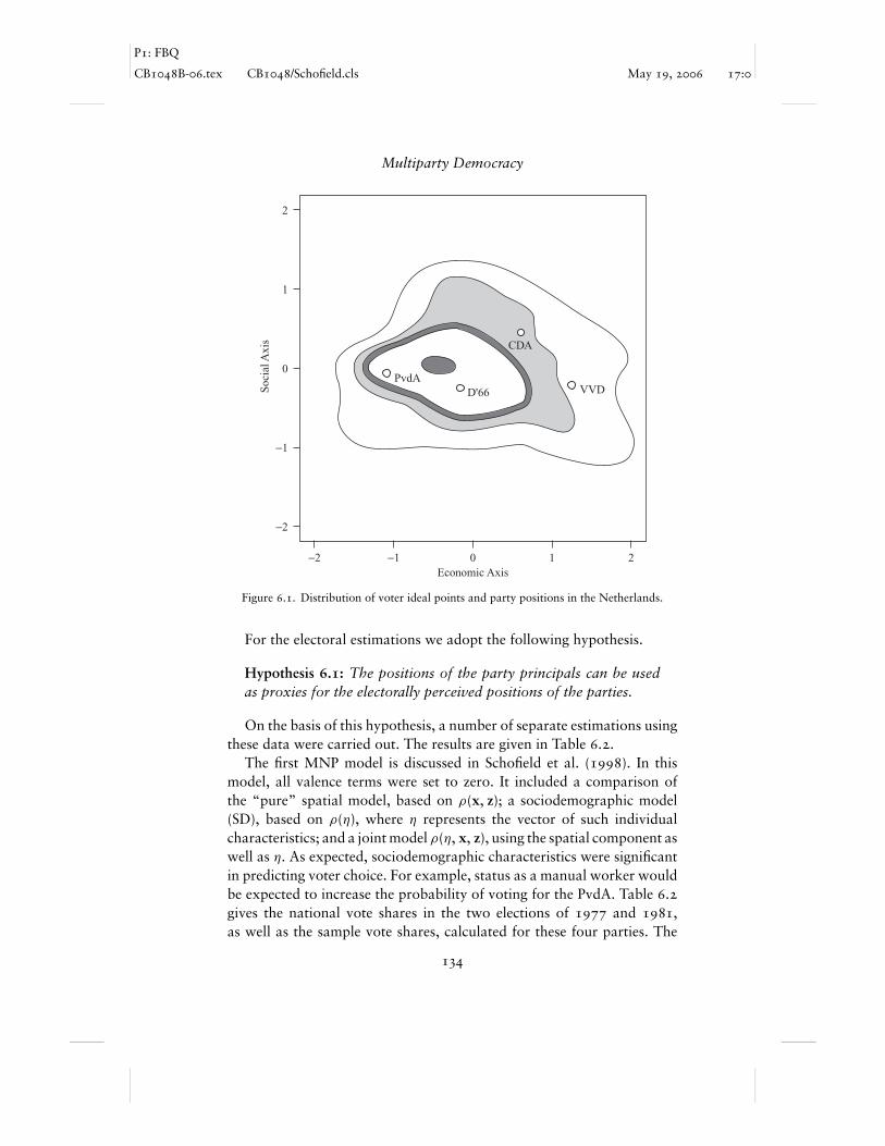
P1: FBQ



D'66 VVD

CDA

PvdA

−2

−2

−1

0

1

2

−1 0 1 2

Economic Axis

Soci

al A

xis

Figure 6.1. Distribution of voter ideal points and party positions in the Netherlands.

For the electoral estimations we adopt the following hypothesis.

Hypothesis 6.1: The positions of the party principals can be usedas proxies for the electorally perceived positions of the parties.

On the basis of this hypothesis, a number of separate estimations usingthese data were carried out. The results are given in Table 6.2.

The first MNP model is discussed in Schofield et al. (1998). In thismodel, all valence terms were set to zero. It included a comparison ofthe “pure” spatial model, based on ρ(x, z); a sociodemographic model(SD), based on ρ(η), where η represents the vector of such individualcharacteristics; and a joint model ρ(η, x, z), using the spatial component aswell as η. As expected, sociodemographic characteristics were significantin predicting voter choice. For example, status as a manual worker wouldbe expected to increase the probability of voting for the PvdA. Table 6.2gives the national vote shares in the two elections of 1977 and 1981,as well as the sample vote shares, calculated for these four parties. The

134

P1: FBQ



Table 6.1. Election Results in the Netherlands,1977–1981.

1977 1981

Party (acronym) (Seats)

Labour (PvdA) 53 44Democrats ’66 (D’66) 8 17Liberals (VVD) 28 26Christian Dem Appeal (CDA) 49 48

(138) (135)Communists (CPN) 2 3Dem ’70 (D70) 1 0Radicals (PPR) 3 3Pacific Socialists (PSP) – 3Reform Federation (RPF) – 2Reform Pol Ass (GDV) 1 1Farmers Party (BP) 1 0State Reform Party (SGP) 3 3

(11) (15)Total 149 150

survey sample vote shares in Table 6.2 can be compared with the party seatdistributions given in Table 6.1. Note that the national vote share of theLabour Party (PvdA) declined from 38 percent in 1977 to 32.4 percentin 1981. Its sample share was 36.9 percent in 1979 and the estimated

Table 6.2. Vote-Shares, Valences, and Spatial Coefficients for EmpiricalModels in the Elections in the Netherlands, 1977–1981.

ConfidenceNational National Interval

Vote, Vote, Sample Esatimated of Vote1977 1981 Vote, Sharea Shareb Valences Valences

Party % % % % % in MNLc in MNPd

D’66 6.1 12.6 10.4 10.6 (6.1, 16.1) 0 0PvdA 38.0 32.4 36.9 35.3 (30.6, 38.9) 1.596 0.622CDA 35.9 35.2 33.8 29.9 (30.1, 40.1) 1.403 0.655VVD 20.0 19.8 18.9 24.2 (14.9, 24.6) 1.015 0.334

β 0.456 0.499 0.737 0.420

a Estimated by an MNP spatial model without valence or SD.b Estimated by an MNP spatial model without valence but with SD.c Estimated by an MNL model with valence without SD.d Estimated by an MNP model with valence without SD.

135

P1: FBQ



expectation from the MNP model, without the SD terms, was 35.3 percentwith a 95 percent confidence interval of (30.9, 39.7).

We have emphasized that the vote-share functions are stochastic vari-ables, with significant variance. This can be illustrated by Figure A6.1in the appendix to this chapter. The estimated shares based on the MNPmodel without SD or valence are fairly close to the sample shares, thoughthe VVD estimation was poor. The log marginal likelihood (LML) wascalculated to be −626. Adding sociodemographic characteristics to theMNP model improved the prediction, as the 95 percent confidence in-tervals in Table 6.2 indicate. The LML changed to −596, so the Bayes’factor (Kass and Raftery, 1995) or the difference between log likelihoodsof the MNP spatial model with SD and without was 30 (= 626 − 596),suggesting that the joint SD model was statistically superior to the purespatial model.

Simulation of these two models found that each of the parties couldhave increased vote share by moving away from their locations inFigure 6.1 toward the electoral mean. We shall show below that thisinference is consistent with Theorem 3.2 when applied to empirical mod-els including valence. Schofield et al. (1998) raised the question: If thepositions given in Figure 6.1 are indeed the party positions, then why dothe parties not approach the electoral center to increase vote share?

To study this question further, an MNL model based on Hypothesis 6.1was estimated to include valence (λ), but without SD. The estimated va-lences are also reported in Table 6.2. Notice that in the model with λ �= 0,the valences are normalized by setting the valence of D’66 to zero. Com-paring this MNL valence model with the MNL model without valencegave a very significant Bayes’ factor of 75, corresponding to a chi-squareof 149. Even comparing it to the above MNP model with SD but withoutvalence, gave a Bayes’ factor of 64 (= 596 − 532). Clearly, the valenceterms increase the statistical likelihood of the voter model.

It should be pointed out that the coefficients, β and λ, are not di-rectly comparable between the MNL and MNP models. The MNL mod-els are based on the (iid) extreme value distribution with error varianceσ 2 = 1

6π2 = 1.6449, while the MNP models are based on some appro-priate normalization for the error difference variances.

Although probit models have theoretical advantages, it would appearfrom the above that the MNL and MNP models give comparable resultsin terms of predictions about party vote shares. To more fully examinethe effect of valence, Tables A6.2 and A6.3 in the appendix present theresult of MNP and MNL estimation for models involving both SD and

136

P1: FBQ



Table 6.3. Log Likelihoods and Eigenvalues in the Dutch Electoral Model.

Convergence EigenvalueSpatial Models Coefficient First Second LMLa

MNL no valence or SDb na na na −606MNL no valence, with SDb na na na −565MNL with valence, no SDc 1.19 −0.18 −0.64 −532MNL with valence and SDc 1.38 −0.04 −0.58 −465MNP without valence or SDd na na na −626MNP without valence, with SDd na na na −596MNP with valence, no SDc 0.75 −0.48 −0.77 −545MNP with valence and SDc 1.55 +0.05 −0.50 −427Non-Spatial, MNP pure SDc −596

a LML = log marginal likelihood.b Based on Schofield and Sened (2005b), using extreme value distribution.c Based on Quinn, Martin, and Whitford (1999).d Based on Schofield, Martin, Quinn, and Whitford (1998).

valence. Quinn et al. (1999) previously computed the Bayes’ factors forthe various models and found the joint spatial MNP and MNL models,ρ(η, x, z), with valence superior to the pure MNP and MNL sociodemo-graphic models ρ(η) without a spatial component. This suggests that theappropriate causal model is one in which SD characteristics (ηi ) influ-ence beliefs (xi ) which in turn affect the probability vector of voter choice(ρi ). Table 6.3 reports the log marginal likelihoods of the eight differentmodels.

An important inference for our argument here is that, as in the case ofIsrael, the explanatory power of each empirical model is much increasedby adding in the valence terms (Stokes, 1963, 1992). Indeed, pairwisecomparison of a model with valence, but without SD, against one withoutvalence, but with SD, suggests that the valence terms, to some degree,substitute for using the individual characteristics of voters. We draw threeconclusions from the log likelihoods presented in Table 6.3.

Conclusion 6.1

(i) There is strong justification for Hypothesis 6.1. The logmarginal likelihoods of all spatial models, when compared withthe pure SD models, indicate that these estimated party positionsprovide a useful basis for modelling electoral choice. Indeed, the95 percent confidence intervals of the β coefficients in TablesA6.2 and A6.3 allow us to reject the hypothesis that the spatialcoefficients are zero.

137

P1: FBQ



(ii) The valence terms are all significant. More importantly, the con-fidence interval on the high-valence party, the PvdA, excludes0, so we can infer that there is a significant valence difference.

(iii) Although the sociodemographic terms are important, their ef-fect can to some extent be captured by valence.

(iv) The valence differences are reduced when SD terms are included.As a consequence, when examining the models to determinewhether convergence is to be expected, it is important to includeSD.

Given that there is evidence for the statistical significance of the esti-mation, we can examine the question of convergence.

It is obvious that if the valence of party j is increased, then the proba-bility that a voter chooses the party also increases. As we have observed,it is not the absolute values of the valences that are relevant but the pair-wise differences in the valences. For estimation purposes we set the lowestvalence of one party to zero. For example, in the MNL model presentedin Table A6.2, the valence of D’66 was normalized to be zero. In theMNP model with SD however it turns out that the religious sociodemo-graphic variable affects the vote choice. The result is that the CDA isestimated to have the lowest valence for this model. We now utilize theresults of the formal model given in Chapter 3 on the basis of the followinghypothesis.

Hypothesis 6.2: The results of the formal model given in Chapter 3are applicable to the analysis of empirical models.

These empirical models are not directly comparable to the formal elec-toral model presented in Chapter 3. In particular, the sociodemographiccomponents are not included in the formal model. In computing the coef-ficients and eigenvalues for the MNL models we used the results given inTheorem 3.1 for the extreme value distribution,�. For the MNP modelsit is necessary to modify the definition of the Hessians to account for er-ror covariance. First, we note that the electoral variance on the first axisis 0.658, whereas on the second it is 0.289. The reason these are bothdifferent from 1.0, is that the normalization was done with respect to thevariance of the delegate points on the first axis.

Table 6.3 also presents the results of the computation of the eigenvaluesof the Hessians at the origin for the lowest-valence party. These compu-tations are presented in a technical appendix to this chapter. Tables A6.1

138

P1: FBQ



and A6.2 in the appendix give the estimation results, including the va-lences for the various parties as well as the sociodemographic coefficientsfor the MNL and MNP models. According to the results of Chapter 3, ifthe convergence coefficient is bounded above by 1.0, then we may arguethat the origin will, for sure, be a local equilibrium. It is evident that theconvergence coefficients of three of the four baseline formal models satisfythis condition. We regard this as strong evidence that the earlier inferencemade by Schofield et al. (1998) about convergence to the electoral originis generally unaffected by the addition of valence to the models. An addi-tional simulation by Quinn and Martin (2002) provides further supportfor the convergence result.

As we have noted, adding sociodemographic terms tends to reduce thevalence coefficients, because these explain less of the voter choice. This hasthe effect of reducing valence difference between high- and low-valenceparties, thus changing the estimated convergence coefficients. However,as Table 6.3 indicates, the effect on the MNL models is trivial. The onlymodel that gives a noncentrist equilibrium is the MNP model with va-lence and SD. Because the correlation between the two electoral axes isnegligible, we can treat the two axes separately. Table 6.3 shows thatfor this model, the eigenvalue of the CDA Hessian on the second axisis negative. This implies that, in local equilibrium, all parties should beat the zero position on the second axis. Because the eigenvalue for theCDA on the economic axis is positive (albeit small), then it is possiblethat its vote-maximizing position will be away from the origin. We can-not predict whether it should move to the right or the left. We can infer,however, that all parties, in equilibrium in this model, should be strungalong the economic axis. It is also the case that the vote-share functionsof the parties were “close” to concave. This can be seen from examiningthe vote probability functions presented in Figures A6.2 and A6.3 (in theappendix to this chapter), based on the positions of the parties given inFigure 6.1. The inference is that the parties should adopt positions on theeconomic axis, but very close to the electoral origin. Note also that, forthree of the four models, because the eigenvalues are typically negative,and “large” in magnitude with respect to the parameters of the variousmodels, then the origin is not only likely to be a local equilibrium withrespect to vote-maximizing, but also the unique Nash equilibrium. Com-paring Figure 6.1 with the predictions of the formal model we thereforeinfer that it is very unlikely that the CDA position is a component of avote-maximizing equilibrium. Although the positions of the PvdA, VVD,

139

P1: FBQ



and D’66 are not in obvious contradiction to the formal interpretation ofthe MNP/SD empirical model, there is evidence that these parties couldhave increased vote share by moving from their presumed positions inFigure 6.1 toward the electoral center. On the basis of Hypothesis 6.2 weare led to the following conclusion.

Conclusion 6.2 It is unlikely that the estimated positions given inFigure 6.1 can belong to a local equilibrium on the basis of an elec-toral model with fixed exogenous valences.

It is possible that the CDA position is one chosen in response to coali-tion risk, as discussed in Section 3.1 in Chapter 3, as well as in the empir-ical illustrations from Israel and Italy in Chapters 4 and 5. There are twodistinct coalition structures relevant to politics in the Netherlands:

D0 = {PvdA,CDA}, {PvdA,VVD}, {CDA,VVD}, and

DPvdA = {PvdA,CDA}, {PvdA,VVD,D’66}, {CDA,VVD,D’66}.

After the May 1977 election, structure D0 can be taken to representthe electoral outcome since the {CDA,VVD} coalition had 77 seats outof 149, and was therefore winning. This coalition did indeed form a gov-ernment, but only after 6 months of negotiation. After the 1981 election,this coalition controlled only 74 seats (out of 150) so we can represent theoutcome by DPvdA. A {PvdA,D’66,CDA} coalition government with 109

seats first formed and then collapsed to a minority {D’66,CDA} govern-ment. A new election had to be called in September 1982. Although thepost-1981 election situation is designated a DPvdA coalition structure, thePvdA could only be at a core position if it adopted a position inside theconvex hull of the {CDA,VVD,D’66} positions. In fact, the heart, giventhe positions in Figure 6.1, together with the seat strengths in 1981, is theconvex hull of the three positions {PvdA,D’66, CDA}. Thus, the minoritycoalition government that did indeed form is compatible with the notionof the heart. Moreover, as Section 3.4 illustrated, the CDA may gain ad-vantage in coalition bargaining if it adopts a radical strategic position onthe second axis.

Notice that the model suggests that there is strong centripetal pres-sure on the PvdA, in terms of adopting a centrist position to both gainseats and possibly control the core policy position. The coefficient forthe PVdA for manual labor given in Appendix Table A6.3, is high andsignificant, suggesting that activists had a centrifugal influence on the pol-icy preferences of the party. This influence appears to have overcome the

140

P1: FBQ



centripetal tendency generated by the formal model with fixed exogenousvalences.

It is also noticeable from the tables that the sociodemographic coeffi-cient associated with religion was highly significant for the CDA, in bothMNL and MNP models. This also suggests that activists concerned aboutpolicy on this axis were influential in determining the CDA position. Weare therefore led to the conclusion that activists for both these partiesgenerated centrifugal forces within each party and that these counteredthe centripetal effect our analysis has shown to be associated with themodel of vote maximizing.

Instead of supposing that valence is exogenously determined at the timeof the election, we now consider the more general hypothesis that valenceis determined by the effect of activists on party support and that thesevalence functions affect the local Nash equilibrium positions that partiesadopt. By contributing support, the party elite enhances the popularity ofthe party. We conjecture that the activist valence terms will not, in fact,be constant, but will be maximized at the center of the distribution of thepositions of the elite or delegates of the parties. This follows because atthis position the contributions of the party activists will be maximized.Consequently, it is plausible that the valence functions will be concavein the positions adopted by the parties. We conjecture that noncentristLNE may exist, and that they may indeed be PNE of this more complexelectoral game.

Our analysis of these elections in the Netherlands suggests the follow-ing conclusion concerning the interplay of electoral and coalition risk inthe strategic calculations of policy-motivated party activists.

Conclusion 6.3 Because the coalition structure DPvdA is advanta-geous to the PvdA, this party should attempt to maximize the prob-ability πPvda that this is the election outcome, and a proxy for this isto maximize the expected vote-share function EPvdA. On the otherhand, while the CDA should attempt to maximize the probability π0

that the coalition structure D0 occurs, it can be rational for the partyto consider the consequences of coalition risk, and choose a posi-tion that allows it to bargain effectively with its probable coalitionpartners.

As mentioned above, the estimates for party locations in Figure 6.1were derived from the ISEIUM delegate surveys. It is a reasonable as-sumption that each delegate of a party has a preferred position to offer tothe electorate. Obviously, there is a calculus involved as delegates optimize

141

P1: FBQ



between their own preferences and the desire to gain votes. The empiricalanalysis of the Netherlands is based on the assumption that the principal’sposition for each party is the one that is offered to the electorate by theparty. In fact, the positions given in Figure 6.1 closely correspond to thepositions estimated by De Vries (1999) using an entirely different method-ology based on policy choices of the parties. These chosen positions thengenerate activist support and the estimated valences. Conclusion 6.3 iscompatible with the more complex model, articulated in Chapter 3, inwhich the party principal chooses a party leader with a different positionbecause of the realization that the chosen position not only affects voteshare, but independently influences the probability that the party will joinin coalition government. These observations suggest the following generalhypothesis on the nature of the centipetal and centrifugal tendencies.

Hypothesis 6.3: The centripetal tendency associated with simplevote maximization in the model with exogenous valence is balancedby:

(i) the motivation of concerned party principals to affect the finalcoalition government policy, and

(ii) the requirement to gain support from activists, thus indirectlyincreasing overall electoral support for the party.

We have suggested in this chapter that there is some evidence that bothinfluences can affect party position. It is difficult to determine which ofthese two effects is more important. However, one way to examine theinfluence of activists is to consider a polity where the coalition effect canbe disregarded. The next two chapters will examine the activist hypothesisin the context of empirical models of elections in Britain and the UnitedStates.

6.3 technical appendix: computation

of eigenvalues

Here we show how the coefficients and eigenvalues given in Table 6.3 canbe computed. As Figure 6.1 indicates, the electoral variance on the firsteconomic axis is v2

1 = 0.658, whereas on the second it is v22 = 0.289. The

covariance is negligible.We can calculate the various coefficients and eigenvalues for the four

models with valence.

142

P1: FBQ



(i) As an illustration of Theorem 3.1, for the extreme value formal modelM(�) without SD we find λd’66 = 0, λPvda = 1.596, λcda = 1.1403,λvvd = 1.015, and β = 0.737. At the joint origin the probability ofvoting for D’66 is

ρd’66 = 11 + e1.596 + e1.403 + e1.015

= 0.074.

Thus, Ad’66 = 0.737(0.852) = 0.627.

Cd’66 = (1.25)(

0.658 00 0.289

)− I =

(−0.18 00 −0.64

)c(�) = 2Ad66(0.658 + 0.289) = 1.187

Since the eigenvalues are −0.18 and −0.64, both negative, it is obvi-ous that the model based on the extreme value distribution gives anLSNE at the joint origin.

(ii) When sociodemographic variables are added to the MNL model(Quinn, Martin, and Whitford, 1999) the valence differences arechanged and we find that the CDA is the lowest-valence party, λcda =−0.784. The other valences are now λvvd = 0.313, λPvda = 2.112 andλd’66 = 0. Using the model � we find β = 0.665. Thus,

ρcda = 11 + e2.896 + e1.097 + e0.784

= 0.04.

Hence, Acda = 0.0665(0.99) = 0.664.

Ccda = (1.33)(

0.658 00 0.289

)− I =

(−0.12 00 −0.61

)c(�, SD) = 1.25.

Again, both eigenvalues are negative and the necessary condition issatisfied. Note the large negative eigenvalue on the second axis incontrast to the small eigenvalue on the first axis.

(iii) With the probit model (without SD), we find λd’66 = 0, λcda =0.655, λPvda = 0.622, λvvd = 0.334, and β = 0.420. Thus, the av-erage valence excluding D’66 is λav(d’66) = 0.537.

143

P1: FBQ



Because the errors have nondiagonal covariance matrix �, we nowcompute the covariance matrix of the difference vector,

ed’66 = (εcda − εd’66, εPvda − εd’66, · · · , εvvd − εd’66). This will bethe symmetric matrix

�d’66(�)

=

⎛⎜⎝ Exp(εcda − εd’66, εcda − εd’66) . .

Exp(εcda − εd’66, εPvda − εd’66) .

Exp(εcda − εd’66, εvvd− εd’66). . Exp(εvvd − εd’66, εvvd − εd’66)

⎞⎟⎠.

Here Exp denotes expectation. Normalization gives the followingmatrix:

�d’66(�) =

⎛⎜⎝ 1.0 −0.06 1.258

−0.06 0.186 0.558

1.258 0.558 0.454

⎞⎟⎠The sum of the terms in this matrix is var (�d’66(�)) = 5.15.

From Theorem 3.2, we find that the Hessian matrix Cd’66 associ-ated with the D’66 is given by

Cd’66(�) =[2Ad’66

(∇n

)− I

],

where ∇n is the electoral covariance matrix and

Ad’66 =[

(p − 1)2β

var (�d’66)

] [λav(d’66) − λd’66

] = 0.39.

Since the number of parties p = 4, we find

Cd’66(�) = (0.78)

(0.658 0

0 0.289

)− I

=(−0.48 0

0 −0.77

)so again the eigenvalues are negative. The convergence coefficient isgiven by

c(�) = 2Ad’66(0.658 + 0.289) = 0.75.

144

P1: FBQ



(iv) Finally, for the MNP model with SD we find λcda = −0.408, λav(cda) =0.443, and β = 0.455. The error difference covariance matrix is

�cda =⎛⎝ 1.0 −0.141 0.170

−0.141 1.383 0.4890.170 0.489 0.936

⎞⎠so var (�cda) = 4.355. Thus,

Acda(�) = 0.8 and Ccda =(

0.05 00 −0.5

).

The coefficient c(�, SD) = 1.55. Obviously the sufficient conditionfails, and one of the eigenvalues is positive. Although the necessary con-dition does not fail, it is clear that the origin is now a saddlepoint for theCDA for this model. Thus, under a pure vote-maximizing model, incorpo-rating sociodemographic characteristics of the voters, the CDA may wellmove away from the origin, along the first, high-variance economic axisso as to gain votes. However, because this eigenvalue on the economicaxis is small in modulus (at least in comparison to the eigenvalue on thesecond axis) in equilibrium we expect the PvdA, D’66 and VVD to beclose to the origin on the second axis. That is, in the equilibrium for theMNP model with SD, all parties should be located on the economic axis.

Naturally there is uncertainty about the correct model. However,the analyses indicate that it is unlikely that the positions in Figure 6.1can constitute a local equilibrium under the assumption of exogeneousvalence.

6.4 empirical appendix

Appendix Table A6.1. Factor Weights for the PolicySpace in the Netherlands.

Issue Dimension 1 Dimension 2

Income distribution +0.510 (10.86) −0.148 (1.92)Terrorism −0.232 (4.28) −0.253 (2.51)Nuclear energy −0.297 (6.74) –Enterprises +0.526 (12.0) –Environment +0.306 (7.46) –MNC +0.612 (12.6) −0.229 (2.42)Abortion +0.327 (5.56) +0.390 (2.45)

Chi-square over d.o.f. = 1.76; Sample size (n) = 529.

145

P1: FBQ



Appendix Table A6.2. Probit Analysis of the 1979 Dutch Survey Data(normalized with respect to D’66).

95% Confidence IntervalModelVariable Party Mean Lower Bound Upper Bound

β (MNP) 0.455 0.341 0.571

Valence PvdA 1.298 0.165 2.433VVD 0.031 −1.116 1.175CDA −0.408 −3.530 2.640

Manual Labour PvdA 0.865 0.377 1.408VVD −0.522 −1.350 0.268CDA 0.537 0.023 1.151

Religion PvdA −0.082 −0.295 0.124VVD −0.012 −0.271 0.242CDA 0.736 0.427 1.108

Income PvdA −0.043 −0.089 0.002VVD 0.059 0.005 0.116CDA 0.021 −0.029 0.068

Town Size PvdA 0.162 −0.073 0.407VVD 0.017 −0.283 0.321CDA −0.236 −0.015 0.517

Education PvdA −0.113 −0.170 −0.054VVD −0.002 −0.074 0.073CDA −0.062 −0.128 0.000

Correctly Predicted % PvdA 61.2VVD 49.5CDA 62.3D66 20.4

MNP Model 56.4Sample Size = 529

Source: Quinn, Martin, and Whitford (1999) and Schofield, Martin, Quinn, and Whitford(1998).

146

P1: FBQ



Appendix Table A6.3. Multinomial Logit Analysis of the 1979 DutchSurvey Data (normalized with respect to D’66).

95% Confidence IntervalModelVariable Party Mean Lower Bound Upper Bound

β (MNL) 0.665 0.557 0.785

Valence PvdA 2.112 1.276 2.927VVD 0.313 −0.920 1.273CDA −0.784 −1.206 −0.265

Manual Labour PvdA 1.406 0.444 2.508VVD −0.547 −1.996 0.937CDA 1.064 0.012 2.330

Religion PvdA 0.080 −0.234 0.408VVD 0.080 −0.236 0.434CDA 1.382 1.070 1.757

Income PvdA −0.056 −0.141 0.038VVD 0.095 0.004 0.201CDA 0.019 −0.065 0.115

Town Size PvdA 0.373 −0.055 0.878VVD 0.221 −0.271 0.774CDA 0.517 0.058 1.044

Education PvdA −0.203 −0.311 −0.086VVD −0.056 −0.173 0.078CDA −0.148 −0.266 −0.033

Correctly Predicted % PvdA 62.5VVD 49.9CDA 62.2D66 19.3MNL Model 55.5

Sample Size = 529

Source: Quinn, Martin, and Whitford (1999) and Schofield, Martin, Quinn, and Whitford(1998).

147

P1: FBQ



0.0 0.1 0.2 0.3 0.4

0.0 0.1 0.2 0.3 0.4

Vote Share

0

5

10

15

20

25

0

5

10

15

20

25

Per

cent

of

Tota

l

Figure A6.1. Estimated stochastic vote-share functions for the Pvda, VVD, CDA, and D’66

(based on 1979 data and the party positions given in Figure 6.1). (Source: Schofield, Martin,Quinn, and Whitford, 1998.)

148

P1: FBQ



1

0.8

0.6

0.4

0.2

0

Pr(

VV

D)

Economic

Social

2

21

10

0−1−1

−2 −2

1

0.8

0.6

0.4

0.2

0

Pr(

CD

A)

Economic

Social

2

21

10

0−1−1

−2 −2

Figure A6.2. Estimated probability functions for voting for the CDA and VVD. (Source:Schofield, Martin, Quinn, and Whitford, 1998.)

149

P1: FBQ



1

0.8

0.6

0.4

0.2

0

Pr(

D'6

6)

Economic

Social

2

21

10

0−1−1

−2 −2

1

0.8

0.6

0.4

0.2

0P

r(P

vdA

)

Economic

Social

2

21

10

0−1−1

−2 −2

Figure A6.3. Estimated probability functions for voting for the Pvda and D’66. (Source:Schofield, Martin, Quinn, and Whitford, 1998.)

150

P1: FBQ


7

Elections in Britain, 1979–2005

The previous chapters on the proportional electoral systems of Israel,Italy, and the Netherlands have considered the hypothesis that the policypositions of parties were chosen not simply to maximize vote-shares, butincorporated strategic concerns over the effect of position on the proba-bility of joining a government coalition. However, this coalition consider-ation is generally not present in the plurality electoral system of Britain.(For convenience we use the term Britain for the United Kingdom). We cantherefore use our electoral model for this polity to determine the degreeto which simple vote-maximization characterizes policy choices. We firstdiscuss the MNP model used by Quinn, Martin, and Whitford (1999) tostudy the election of 1979 in Britain, and then extend the analysis to MNLmodels of the 1992 and 1997 elections. In all three cases the estimated pa-rameters give low convergence coefficients. Theorem 3.1 then implies thatconvergence to the electoral center should have occurred under vote-sharemaximization.

Since there is no evidence of convergence by the major parties in Britain(Alvarez, Nagler, and Bowler, 2000) we develop the activist valence modelmentioned in the previous chapter. We now allow the contributions ofactivists to indirectly enhance the valence of the party leader. The principalresult we offer shows that there is a tradeoff to be made between theleader’s “exogenous” valence and this “indirect” valence induced by theactivists for the party.

We suggest that the valence of the Labour Party, under Tony Blair,increased in the period up to 1997. As a consequence of the relative de-cline of the Conservative Party leader’s valence, the Conservative Partywas obliged to depend increasingly on activist support, forcing it toadopt a more radical position. Conversely, Blair’s high valence weakened

151

P1: FBQ



Liberal

Conservative

Labour

Economic Dimension

0

1

2

−2

−2

−1

−1 10 2

Gov

ernm

enta

l S

cope

Figure 7.1. Distribution of voter ideal points and party positions in Britain in the 1979

election, for a two-dimensional model, showing the highest density contours of the samplevoter distribution at the 95%, 75%, 50%, and 10% levels.

his dependence on activists and allowed him to adopt a more centrist,election-winning position.

We propose the following hypothesis:

Hypothesis 7.1: If policy choices in a plurality electoral system ap-pear to conflict with vote-maximization in the simple exogenousvalence model, then this is due to the influence of activists for theparty.

7.1 the elections of 1979, 1992, and 1997

We now examine this indirect role played by activists in determining thepolicy decisions of parties in Britain. To set the scene, Figure 7.1 presentsthe estimated positions of the party principals of the three major partiesat the election of 1979, in a two-dimensional policy space.

152

P1: FBQ



Just as in the case of the Netherlands, the estimation used the mid-dle level Elites Study (ISEIUM, 1983) coupled with the Rabier-Inglehart(1981) Eurobarometer study (see Quinn, Martin, and Whitford, 1999,and Schofield, 2005b for further details.) The electoral variances were0.605 on the first axis and 0.37 on the second, giving a total variance of0.975. For the MNL model incorporating sociodemographic characteris-tics, the spatial coefficient was β = 0.27 and the convergence coefficient

Table 7.1. Elections in Britain in 2005, 2001, 1997, and1992.

2005 Seats Seats % Vote %

PartyLabour Party (LAB) 356 55.2 35.3Conservative Party (CON) 198 30.7 32.3Liberal Democrats Party (LIB) 62 9.6 22.1Total: major parties 615 95.2 89.7Scottish National Party (SNP) 6 1.0 1.5Plaid Cymru (PC) 3 0.5 0.6Independent, Respect, KHHC 3 0.5 0.3Northern Ireland in total, 18 2.8 2.5comprising:

Ulster Unionists (UU) 1 0.5Democratic Union 9 0.9SDLP 3 0.5Sinn Fein 5 0.6

Total 646


PartyLabour Party (LAB) 412 62.6 40.1Conservative Party (CON) 166 25.1 31.7Liberal Democrats Party (LIB) 52 7.8 18.6Total: major parties 630 97.5 90.4Scottish National Party (SNP) 5 0.8 1.8Plaid Cymru (PC) 4 0.6 0.7Independent 1Northern Ireland in total, 18 2.8comprising:

Ulster Unionists (UU) 6Democratic Union 5SDLP 3Sinn Fein 4

(continued)

153

P1: FBQ



Table 7.1. (continued)


PartyLabour Party (LAB) 419 63.6 44.4Conservative Party (CONS) 165 25.0 31.4Liberal Democrats Party (LIB) 46 6.9 17.2Total: major parties 630 95.5 93.0Scottish National Party (SNP) 6 0.9 2.0Plaid Cymru (PC) 4 0.6 0.5Independent 1Northern Ireland in total, 18 2.7comprising:

Ulster Unionists (UU) 10UK Unionists 1Democratic Union 2SDLP 3Sinn Fein 2


PartyLabour Party (LAB) 271 41.6 34.5Conservative Party (CON) 336 51.6 41.9Liberal Democrats Party (LIB) 20 3.1 17.9Total: major parties 627 94.3Scottish National Party (SNP) 3 0.5 1.9Plaid Cymru (PC) 4 0.6 0.5Northern Ireland 17 2.6 3.3

was calculated to be 0.26. The eigenvalues of the Hessians of all partiesat the origin were then negative. With the MNP model the coefficient waseven smaller—0.08—and the eigenvalues of all parties close to −1.0. Asin the previous example from the Netherlands, the origin was an LSNE.Indeed, the estimation suggests that the origin was a PSNE. This inferenceconflicts with the estimated positions of the parties given in Figure 7.1.

To pursue this contradiction further, we now consider more recentelections. Table 7.1 gives details on the elections of 1992, 1997, 2001,and 2005 in Britain. As usual with plurality electoral rules, small gainsin vote-share lead to large gains in seat share. British National ElectionSurveys (British Election Studies, 1992, 1997) were used to construct asingle-factor model of the voter distribution (see Table 7.3 for the surveyquestions). We shall call this factor the economic dimension. Note that

154

P1: FBQ



Table 7.2. Factor weights from the British NationalElection Survey for 1997.

Britain (without Scotland), 1997

Issue Factor weights

1. Unemployment and Inflation 0.2652. Taxation and Services 0.2233. Nationalization 0.2254. Redistribution 0.3185. European Community 0.0876. Women’s Rights 0.149

Scotland, 1997

Issue Factor weights

1. Unemployment and Inflation 0.1272. Taxation and Services 0.1043. Nationalization 0.1564. Redistribution 0.5805. European Community 0.0086. Women’s Rights 0.1377. Scottish Nationalism 0.101

Table 7.3. Question Wordings for the British National ElectionSurveys for 1997.

1. Do you feel that the government’s top priority should be getting peopleback to work, keeping prices down, or somewhere in between?

2. Do you feel the government should raise taxes and spend more moneyon health and social services, or do you feel they should cut taxes andspend less on these services?

3. Do you feel the government should nationalize or privatize moreindustries?

4. Do you feel the government should be more concerned with equalizingpeople’s incomes, or less concerned?

5. Do you feel Britain should unite with the European Union or protect itsindependence from the European Union?

6. Do you feel women should share an equal role in business, industry, andgovernment, or do you feel a woman’s place is in the home?

7. Do you feel Scotland should a) become independent, separate from theUK and the European Union, b) become independent, separate from theUK, but a part of the European Union, c) remain part of the UK, with itsown elected assembly, with taxation and spending powers, or d) remainas it is?

155

P1: FBQ



−2 −1 0

Lab Lib Con

1992

0.0

0.2

0.4

0.6

0.8

1.0

1Economics

Den

sity

of

All

Vote

rs

2

Lab Lib Con

1997

−2 −1 0

0.0

0.2

0.4

0.6

0.8

1.0

1Economics

Den

sity

of

All

Vote

rs

2

Figure 7.2. Estimated party positions in the British Parliament in 1992 and 1997, for a one-dimensional model (based on the National Election Survey and voter perceptions) showingthe estimated density function (of all voters outside Scotland).

Scottish Nationalism is, of course, an issue in Scotland but not in the restof the country.

Table 7.2 gives the factor weights for 1997 for Britain (subdividedinto Britain without Scotland, and Scotland alone). The 1992 weightswere very similar. Figure 7.2 presents the estimated distribution of voterideal points (for voters outside Scotland), on the basis of this single eco-nomic dimension. The voter distribution in Scotland was somewhat sim-ilar, though less symmetric, and skewed to the left. The party positionsfor the Labour Party (Lab), Liberal Democrat Party (Lib), Conservative

156

P1: FBQ



Table 7.4. Sample and Estimation Data for Elections in Britain, 1992–1997.

Sample Confidence Correct1992 % Coefficients interval prediction %

UK without β = 0.56 [0.50, 0.63] 50.0Scotland

Conservative 49.3 λ = 1.58 [1.38, 1.75] 62.9Labour 32.4 λ = 0.58 [0.40, 0.76] 47.4Liberals 18.2 λ = 0.00 19.7

Scotland β = 0.50 [0.31, 0.67] 35.6Conservative 30.2 λ = 1.68 [1.18, 2.21] 48.6Labour 31.4 λ = 0.91 [0.38, 1.51] 37.2SNP 25.9 λ = 0.77 [0.26, 1.30] 29.5Liberals 12.3 λ = 0.00 12.8

Sample Confidence Correct1997 % Coefficients interval prediction %

UK without β = 0.50 [0.44, 0.56] 45.7Scotland

Conservative 31.9 λ = 1.24 [1.03, 1.44] 45.2Labour 49.6 λ = 0.97 [0.85, 1.07] 56.1Liberals 18.5 λ = 0.00 19.0

Scotland β = 0.50 [0.40, 0.64] 40.5Conservative 14.2 λ = 0.92 [0.58, 1.24] 33.7Labour 52.7 λ = 1.33 [1.10, 1.57] 56.3SNP 20.4 λ = 0.42 [0.16, 0.72] 21.5Liberals 12.5 λ = 0.00 12.8

Party (Con), and Scottish National Party (SNP) were inferred by takingaverage voter perceptions of the locations of these parties.

The positions Lab, Lib, and Con in the two election years (for votersoutside Scotland) were given by the vectors

z92 = (zlab, zlib, zcon) = (−0.65, −0.11, +1.12) (7.1)

z97 = (−0.2, +0.06, +1.33). (7.2)

See Figure 7.2.In 1992 the SNP position was perceived to be zsnp = −0.3, and in 1997

it was +0.14.Using these data, MNL models were constructed for the four cases in

1992 and 1997, for Scotland and the rest of the country. These modelsallowed us to estimate the exogenous valence terms, as in Table 7.4.

157

P1: FBQ



The estimated coefficients in the two elections were

(λcon, λlab, λlib, β)1997 = (+1.24, 0.97, 0.0, 0.5) (7.3)

(λcon, λlab, λlib, β)1992 = (+1.58, 0.58, 0.0, 0.56) (7.4)

These estimates are compatible with extensive survey research whichdemonstrates the relationship between positive attitudes to party leadersand voting intentions (King, 2002; Clarke et al., 2004). Notice that theConservative Party valence fell, while that of the Labour Party rose. Thesechanges in valences are presumed to be independent of the apparent per-ceived move away from the electoral center by the Conservative Party,and the perceived move toward the electoral center by the Labour Party.

The empirical model was relatively successful, in the sense thatthe model prediction success rate was approximately 50 percent. AsTable 7.4 indicates, the 95 percent confidence intervals for the valencesof the Labour Party and Conservative Party exclude zero. We infer thatthe valence differences between the Liberal Democrats and both Labourand the Conservatives are non-zero. The log marginal likelihood of the1997 MNL model with valence was −531, giving a Bayes’ factor of 75

over the MNL model without valence. For Britain without Scotland in1997 we can use the results of Chapter 3 to compute the convergencecoefficient for these two elections. Because the model is MNL we use theformal model based on the Type I extreme value distribution. Since themodel is one-dimensional, the electoral variance on the single axis is nor-malized to be 1.0. Because the valence of Lib is normalized to be zero, wefind that for 1997 the eigenvalue of the Hessian of the Liberal DemocratParty at the joint origin is −0.28. A similar value of −0.18 was obtainedfor 1992.

The results of Chapter 3 thus imply convergence for the formal model.Even using the upper estimated bound of the parameters, we obtain similarestimates for the eigenvalues. Thus, on the basis of the formal model, wecan assert with a high degree of certainty that the low-valence party, theLiberal Democrats, can be located at an LNE at the origin if all otherparties also locate there. According to the model, the vote-share of theLiberal Democrat Party would have been 13 percent in 1992, or 14 percentin 1997, had the other two parties located at the origin in these elections.Because the two major parties did not locate at the origin, the actual vote-share of 17 percent to 18 percent for the Liberals is compatible with theseestimates.

Thus, under the assumptions of fixed or exogenous valence, vote-maximization, and unidimensionality, a version of the mean voter theorem

158

P1: FBQ



should have been valid for the British elections of 1992 and 1997.Although Figure 7.2 indicates that a position close to the center wasadopted (or seen to be adopted) by the Liberal Democrats in 1992 and1997, this was not so obvious for the Labour Party, and was clearly falsefor the Conservative Party. Indeed, for both subsets of the electorate(within Scotland and outside), the Labour Party was perceived to ap-proach closer to the center between 1992 and 1997, but the ConservativeParty was perceived to become more radical.

7.2 estimating the influence of activists

In an attempt to account for the obvious disparity between the conclu-sions of the vote-maximization model and party location, we consideredthe hypothesis that party location was determined by party elites. As weproposed in the discussion of the Netherlands, the location of the dele-gates or elite positions can be used to determine the position of maximumactivist support for each party. This, in turn, will determine the preciseequilibrium location of each party. While activists contribute time andmoney and affect overall political support for the party, the activist loca-tions will tend to be more radical than the average voter. This presentsthe party leader with a complex “optimization problem.” We use the ac-tivist valence argument to offer a conjecture about how party leaders dealwith this problem by choosing differing policy positions to present to theelectorate (Robertson, 1976).

Figure 7.3 gives the estimated voter distribution in the British electionof 1997, based on the British National Election Survey but using the twodimensions obtained from factor analysis. (See Table 7.2 for the factorweight associated with this second “European” dimension.) Positions ofMPs of each party were estimated on the basis of an MP sample responseto the British National Election questionnaire. For each party, the averageof the party MP positions was used as an estimate of the position of eachparty “principal.” The estimated positions of individual MPs in the surveyare given in Figure 7.4.

A considerable difference among ideal points of MPs within partiescan be observed. The second, “vertical,” axis in Figure 7.3 is determinedby “pro-Europe” versus “pro-British” (or “anti-Europe”) attitudes. Theparty principal positions of Labour (LAB) and Conservatives (CONS)are separated on both axes, but more so on the Europe axis. The smallnumber of Ulster Unionists (UU) appeared to be similar to other Conser-vatives, but more extreme on the pro-British axis. The single sampled MP

159

P1: FBQ



UU

SNP

LAB

−2

−2

−1

0

1

2Pro-Britain

Pro-Europe

Pro-Labour Pro-CapitalEconomic Issues

−1 0

PC LIB

CONS

1

Nat

ion

alis

m

2

Figure 7.3. Estimated party positions in the British Parliament for a two-dimensional modelfor 1997 (based on MP survey data and the National Election Survey) showing high-est density contours of the voter sample distribution at the 95%, 75%, 50%, and 10%levels.

for Plaid Cymru (PC, from Wales) was similar to other left, pro-EuropeLabour MPs, while the single sampled member of the SNP (from Scot-land) also resembled other Labour MPs who were less pro-Europe. Thefifteen sampled Liberal Democrats (with principal position denoted LIB)were all somewhat left of center, and very pro-Europe.

The empirical estimates presented above, and those based on the one-dimensional model, suggest that the Labour valence had increased from1992 to 1997. In terms of this empirical model, this increase was inde-pendent of the greater voter support induced by the party moving closerto the electoral center under Tony Blair. We now consider the followinghypothesis.

160

P1: FBQ



SNPPC

CONS LAB

Economic Dimension

Nat

ional

ism

Dim

ensi

on

0 0

0

1 1

1

2 23 3−1 −1

−1

−2

0

1

−1

−2

LIB

UU

0 1 2 3−1

Key

PC: Plaid Cymru ( Welsh Nationalist Party)SNP: Scottish Nationalist PartyUU: Ulster UnionistsCONS: Conservative PartyLAB: Labour Party LIB: Liberal Democrat Party

Figure 7.4. Estimated MP positions in the British Parliament in 1997, based on MP surveydata and a two-dimensional factor model derived from the National Election Survey.

Hypothesis 7.2: The apparent move by the Labour Party toward theelectoral center between 1992 and 1997 was a consequence of theincrease of the valence of the leader of the party, rather than a causeof this increase.

To develop this hypothesis, we shall assume that the party principalpositions given in Figure 7.3 do indeed represent in some sense the averagelocation of party activists. We then attempt to model the influence ofactivists on optimal party position.

161

P1: FBQ



Note first that the positions perceived by the electorate in 1997 andgiven by the vector z97 = (−0.2, +0.06, +1.33) are very close indeed tothe projections of the positions of the party principals onto the economicaxis in Figure 7.3. This leads us to infer that the party principal positionsdo influence perceived party positions. Just as we did in Chapter 6, we canexamine whether the party principal positions can be a local equilibriumto a simple vote-maximizing game. The Technical Appendix to this chap-ter shows that when we include the second European axis then the LiberalParty eigenvalue on this axis is positive. This calculation is based on zeroelectoral covariance between the two axes, and the greater electoral vari-ance on the second “Europe” axis. In other words, if all three partieswere at the electoral center, then the positive eigenvalue of the Hessian onthe second dimension would give the Liberal Democrat Party leader anincentive to change position, but only on the second axis. We may inferthat the average preferred position of the party MPs would induce theparty leader to adopt a pro-Europe position. If the Liberal Party were toadopt a pro-Europe position as indicated by its principal’s position, thenthe logic of vote-maximization would induce the Labour Party leader tomake a similar move. Thus, the positions LAB and LIB are compatiblewith the simple vote-model with exogenous valence.

This conclusion still leaves unexplained the perceived location of theConservative Party (CONS).

Under the assumptions of the fixed valence model, the ConservativeParty should have adopted a vote-maximizing position closer to the originthan did the Labour Party. We suggest that the Conservative Party didnot converge on the mean because of the subtle interrelationship betweenexogenous valence and activist valence. Blair’s increasing valence in theperiod up to 1997 resulted in a decrease in the importance of the activistsin the party (Seyd and Whiteley, 2002). This led to a more centrist vote-maximizing strategy by Labour, associated with a larger “electoral sphereof influence.” In contrast, decreasing Conservative leader valence led toan increase in the importance of activists. To maintain grassroots support,the Conservatives were forced to adopt quite radical positions, both onthe question of Europe and on economic issues.

Schofield (2003b, 2004, 2005a,b) presents a formal analysis of thesediffering valence effects. It is consistent with this more general model thatall parties at the election of 1997 were at vote-maximizing positions. Wenow turn to this extension.

In essence, the model we propose suggests that if the leader of oneparty benefits from increasing valence, then the party’s optimal strategy

162

P1: FBQ



will be to move toward the political center in order to take advantage ofthe electoral benefits. In contrast, a party, such as the Liberal DemocratParty, whose leader is unable to take advantage of high valence, cannotexpect to gain commanding electoral support, even when the party adoptsa centrist position.

In the following section, we present the underlying formal electoralmodel that we use, and state the constraint on the model parameters,which is sufficient for concavity and thus for existence of a noncentristpure strategy Nash equilibrium. Indeed we show that the joint vote-maximizing positions will generally not be at the voter mean. We brieflydiscuss the optimality condition when both “exogenous” valence and“activist” valence are involved, and indicate why activists become morerelevant when leader valence falls.

7.3 a formal model of vote-maximizing

with activists

We return briefly to the model we introduced in Chapter 3 so that we canextend it here to account for noncentrist political choice in the case ofBritain.

In the model with valence, the stochastic element is associated with theweight given by each voter i to the perceived valence of the party leader.We now allow valence to be indirectly affected by party position.

Definition 7.1 The formal model M(λ, A, μ;Ψ)

In the general valence model, let z = (z1, . . . , zp) ∈ Xp be a typical vec-tor of policy positions. Given z, each voter i is described by a vectorui (xi , z) = (ui1(xi , z1), . . . , uip(xi , zp)), where the utility of voter i , at theparty declaration vector z, is given by

ui j (xi , z j ) = λ j + μ j (z j ) − Ai j (xi , z j ) + ε j . (7.5)

The term Ai j (xi , z j ) is derived from a general metric. The errors {ε j } areagain assumed to be distributed by the Type I extreme value distribution,�. For party j , the vote-share E j is the expectation

1n

∑i

ρi j .

For convenience, in terminology below we shall refer to the effect of can-didate strategies on the expected vote-share function E j , through changein μ j (z j ), as the valence component of the vote. Change in E j through

163

P1: FBQ



the effect on the policy distance measure Ai j (xi , z j ) we shall refer to asthe nonvalence, or policy component. We discuss this activist model be-low. One important modification of the pure spatial model that we makeis that the salience of different policy dimensions may vary among theelectorate. More precisely, we assume that

Ai j (xi , z j ) = ||xi − z j ||2i (7.6)

may vary with different i.The term μ j (z j ) is called the activist valence of the party. Notice that

activist valence is now a function of the leader position z j . To distinguishthe two forms of valence, we call λ j the exogenous valence.

We propose an extension of the model presented in Chapter 3 to includeactivist valence. In this new model the first-order condition for vote-sharemaximization is not satisfied at the mean. We now briefly sketch theprocedure for determining the first-order condition. The choice of voteri now depends on the comparison vector

gi j (z) = (..., δ2ik − δ2

i j − λk + λ j − μk(zk) + μ j (z j ), . . .) : for all k �= j),(7.7)

where δ2i j = ||xi − z j ||2i , etc.

Section 7.6.2 in the appendix to this chapter shows that the first-ordersolution z∗

j is given by the balance equation

z∗j = 1

2dμ j

dz j+

n∑i=1

αi j xi . (7.8)

In this equation, the coefficients αi j depend on {λk, λ j , μk(zk), μ j (z j )}and are increasing in {λ j , μ j (z j )} and decreasing in {λk, μk(zk) : k �= j}.The actual coefficients will depend on the distribution assumption madeon the errors. For convenience let us write∑

i

αi j xi = dE∗j

dz j. (7.9)

Then we can rewrite the balance equation as[dE∗j

dz j− z∗

j

]+ 1

2dμ j

dz j= 0. (7.10)

The bracketed term on the left of this expression is the marginal elec-toral pull and is a gradient vector pointing toward the weighted electoralmean. This weighted electoral mean is simply that point at which the elec-toral pull is zero. In the case μ j = 0 for all j, then for each party j , it is

164

P1: FBQ



obvious that all αi j are identical, so z∗j = 1

nxi . This gives, as in the proofof Theorem 3.1, the point where the marginal electoral pull is zero.

The vector dμ j

dz j“points toward” the position at which the party’s ac-

tivist valence is maximized. We may term this vector the (marginal) activistpull. When this marginal or gradient vector dμ j

dz jis increased, then the equi-

librium is pulled away from the weighted electoral mean, and we can saythe “activist effect” is increased. On the other hand, if the activist va-lence functions are fixed, but λ j is increased, or the terms {λk : k �= j} are

decreased, then the vectordE∗

j

dz jincreases in magnitude, the equilibrium is

pulled toward the weighted electoral mean, and we can say the “electoraleffect” is increased.

When the first-order condition is satisfied for all parties at the vectorz* then say z* is a balance solution or satisfies the balance condition.

Moreover, if the activist effect is concave, then the second-order con-dition (or the negative definiteness of the Hessian of the “activist pull”)will guarantee that a vector z* that satisfies the balance condition willbe an LSNE. Schofield (2003b) proved this result for iind errors. Theseobservations then give the following theorem.

Theorem 7.1 Consider the vote-maximization modelM(λ, A, μ; �) based on a disturbance distribution � and includingboth exogenous and activist valences. The first-order condition forz∗ to be an equilibrium is that it satisfies the balance condition. Otherthings being equal, the equilibrium position z∗

j will be closer to aweighted electoral mean the greater is the party’s exogenous valence,λ j . Conversely, if the activist valence function μ j is increased, dueto the greater willingness of activists to contribute to the party, thenearer will z∗

j be to the activist-preferred position. If all activistvalence functions are highly concave, in the sense of having negativeeigenvalues of sufficiently great magnitude, then the balance solutionwill be a PNE.

The proof of this result is given in Section 7.6.2 in the TechnicalAppendix.

Figure 7.5 illustrates this result, in a two-dimensional policy space de-rived from the data as presented in Figure 7.3. We have observed thatoverall Conservative valence dropped from 1.58 in 1992 to 1.24 in 1997,while the Labour valence increased from 0.58 to 0.97. These estimatedvalences include both exogenous valence terms for the parties and the ac-tivist component. Nonetheless, the data presented in Clarke et al., (1998,

165

P1: FBQ



Pro-Britain

Pro-Britain indifference curve

B

Activist pull

Electoral pull

Politicalcleavageline

Capital

Pro-Europeindifference curve

E

Pro-Europe

Optimal Labour

position

Contract curvebetween economicleftists andpro-Europe activist

Economic conservativeindifference curve

Optimal Conservative position

Labour

ECONOMICDIMENSION

Economic leftistindifference curve

L C

Figure 7.5. Illustration of vote-maximizing party positions of the Conservative and Labourleaders for a two-dimensional model.

2004) suggest that the Labour exogenous valence λlab, due to Blair, rosein this period. Conversely, the relative exogenous term λcon for the Con-servatives fell. Since the coefficients in the equation for the electoral pullfor the Conservative Party depend on λcon − λlab, the effect would be toincrease the marginal effect of activism for the Conservative Party, andpull the optimal position away from the party’s weighted electoral mean.

Indeed, it is possible to include the effect of two potential activist groupsfor the Conservative Party: one “pro-British,” centered at the positionmarked B in Figure 7.5 and one “pro-Capital,” marked C in the figure. Theoptimal Conservative position will be determined by a version of thebalance equation, but one that equates the “electoral pull” against the two“activist pulls.” Since the electoral pull fell between the elections, theoptimal position zcon* will be one that is “closer” to the locus of pointsthat generates the greatest activist support. This locus is where the joint

166

P1: FBQ



marginal activist pull is zero. This locus of points can be called the activistcontract curve for the Conservative Party.

Note that in Figure 7.5, the indifference curves of representative ac-tivists for the parties are described by ellipses. This is meant to indicatethat preferences of different activists on the two dimensions may accorddifferent saliences to the policy axes. The activist contract curve givenin the figure, for Labour, say, is the locus of points satisfying the activistequation dμlab

dzlab= 0. This curve represents the balance of power between

Labour supporters most interested in economic issues concerning labour(centered at L in the figure) and those more interested in Europe (centeredat E). The optimal positions for the two parties will be at appropriatepositions that satisfy the balance condition. In other words, each optimalposition will lie on a locus generated by the respective activist contractcurves and the party’s weighted electoral mean point where the electoralpull is zero. As the theorem states, because the coefficients of the weightedelectoral mean for Labour depend on λlab − λcon, we would expect a risein this difference to pull the party “nearer” the electoral origin.

In Chapter 8 we apply this model and show that the equation for thiscontract curve from the preferred pro-European point (sE, tE) to the pro-labour point (sL, tL) is given by the equation

(y − tE)(x − sE)

= S(y − tL)(x − sL)

(7.11)

where

S = b2

a2.e2

f 2. (7.12)

Here, ba > 1 measures the degree to which activists for the Labour

Party are more concerned with economics rather than with Europe, whileef > 1 measures the opposite ratio for Europe activists. Obviously, withidentical saliences, S = 1, and the contract curve is linear.

The “political cleavage line” in the figure is a representation of theelectoral dividing line if there were only the two parties in the election.The weighted electoral mean should lie on the intersection of the politicalcleavage line and the line connecting the two party positions.

As Theorem 7.1 indicates, when the relative exogenous valence for aparty falls, then the optimal party position will approach the activist con-tract curve. Moreover, the optimal position on this contract curve willdepend on the relative intensity of political preferences of the activists ofeach party. For example, if grassroots “pro-British” Conservative Party

167

P1: FBQ



activists have intense preferences on this dimension, then this feature willbe reflected in the activist contract curve and thus in the optimal Conser-vative position.

For the Labour Party, it seems clear that two effects are present. Blair’shigh exogenous valence gave an optimal Labour Party position that wascloser to the electoral center than the optimal position of the Conserva-tive Party. Moreover, this affected the balance between pro-Labour or“old left” activists in the party and “New Labour” activists, concernedwith modernizing the party through a European style “social democratic”perspective. This inference, based on our theoretical model, is compatiblewith Blair’s successful attempts to bring “New Labour” members intothe party (See Seyd and Whiteley, 2002, for documentation). To relatethis analysis to the idea of a party principal offered in earlier chapters, wemay say that the both parties are characterized by competition betweenopposed party principals, located at L and E for Labour, and at C and Bfor the Conservative Party.

7.4 activist and exogenous valence

Our purpose in introducing the notions of “exogenous valence” and “ac-tivist valence” has been to explore the possibility that the relationshipbetween the party and the potential party activists will be affected by theexogenous valence of the leader. Party leaders can either exploit changesin their valence, or become victims of such changes. The theoretical frame-work that we have offered is intended to provide an explanation for theseemingly radical policy choices of the Labour Party during the periodof Conservative government from 1979 until about 1992. By radical wemean simply that the party adopted positions that appeared to be farfrom the electoral center. In recent years, the Conservative Party appearsto have adopted policy choices that are radical, but on the European axis.According to the model just presented, these policy choices are perfectlyrational in that they are designed to maximize votes. A similar argumentwill be applied in the next chapter to apparently radical policy choices inthe Republican–Democrat electoral competition in the United States.

Although the elections of the 1980s are not examined here, we conjec-ture that, during this period, the electorate, in general, viewed MargaretThatcher as more competent than her rival Neil Kinnock. In the modelthat we have proposed, Thatcher’s perceived degree of competence, or ex-ogenous popularity valence, was relatively independent of the particularpolicies that she put forward for the party. It is, of course, a simplification

168

P1: FBQ



to assume that the perception of her competence was independent of thepolicy preferences, or the sociodemographic characteristics, of individualvoters. In principle it would be possible to refine the above model byexamining optimal party positions with respect to these variables.

The simple model presented above suggests that the low average per-ception of Kinnock’s competence, in comparison to Thatcher’s, obligedhim to pay great weight to the activists within the Labour Party. Asa consequence, both Labour and Conservative Parties adopted vote-maximizing, but relatively radical, positions far from the electoral center.Even though the Liberal or Liberal Democrat Party adopted a centristposition, its low exogenous valence kept it in the third party position.

It is possible that Thatcher was deposed from the leadership of theConservative Party precisely because her falling personal valence led togreater electoral weight for powerful activist elements in her party. Indeed,the party mandarins may have understood the nature of the balance con-dition, although Thatcher probably denied it. We have, somewhat simplis-tically, characterized the optimal activist intraparty balance in terms of acontract curve. In fact, the process by which the party leader is selected bythe competing party principals can be expected to be highly contentious.

During Major’s tenure as leader of the Conservative Party, the debacleover the value of sterling and the change to John Smith as the Labour Partyleader led to a transformation in the relative exogenous valences of thetwo parties. Clarke, Stewart, and Whiteley (1998) note the rapid changein voter intentions in favor of Labour when John Smith took over fromKinnock, in July of 1992, and again when Blair took over the leadershipof the party in July of 1994. Time-series analyses of voter intentions showquite clearly how these are determined by perceptions of governmentcompetence in dealing with economic problems (see also Seyd and White-ley, 1992; Clarke et al., 1995, 1997, 1998; Clarke, Sanders et al., 2004).

In addition, however, voting intentions will be affected by judgmentsabout the presumed “fitness” of the party leaders. Our estimates of theseaverage electoral judgments suggest that Tony Blair was perceived to bemuch more fit than earlier Labour Party leaders to head the government.By themselves, however these changes in electoral judgments would nothave given the Labour Party such a clear majority in 1997. The modelthat we propose suggests that Blair’s enhanced valence made it possiblefor him to persuade the “Old Labour” activists of the party that it wasin the best interests of the party to move to a much more centrist policyposition. This transformation of the party was electorally credible, andled to the overwhelming Labour Party victory in 1997.

169

P1: FBQ



Up until 2003, the Conservative Party leaders, William Hague and IainDuncan Smith, seemed to have been deemed by the electorate to have lowexogenous valence. One way to estimate exogenous valence of a leader isto take as a proxy the difference between the proportion of the electoratewho are satisfied with the leader and those who are not. The valenceproxy for Blair in 1997 was about 0.5, whereas the valence proxy forHague was about −0.2. In 2002, the valence proxy for Duncan Smithwas about −0.1. Consistent with our model and with the estimationsgiven above, Conservative Party activists have exerted their power tomove the party further from the electoral origin. This led, first of all, tothe Conservative Party defeat in 2001, and to the struggle inside the partyover which activist group would construct the party policy in the future.The leadership contest was won by Michael Howard in October 2003.By the election of 2005, the proxies of both Howard, the ConservativeParty leader, and Blair, were similar at about −0.2.

Recent international events, and Blair’s responses to them, appear tohave decreased his personal valence. As Table 7.1 indicates, in May 2005

the Labour Party lost nearly sixty seats that it had won in 2001. Thedrop of nearly 6 percent of the popular vote would appear to be entirelydue to the increased electoral mistrust caused by Blair’s handling of theIraq situation. There has been a move to force Blair to resign in favor ofGordon Brown, but at the time of writing, it is fairly subdued.

While the number of seats for the Conservatives increased by thirty overthe 2001 figure, the popular vote-share hardly increased over the levels for1997 and 2001. This was obviously the reason that Howard announcedhis resignation “sooner rather than later” from the party leadership im-mediately after the election. In December, 2005, the party chose a newleader, David Cameron. It remains to be seen whether the electorate willjudge him to be a competent leader.

The model proposed here suggests that this change in Blair’s valencefrom 2001 to 2005 may induce conflict inside the Labour Party, betweeneconomic activists, on the one hand, and pro-Europe social democratson the other. Indeed, a third axis of political choice, concerned with theMiddle East, may have come into existence recently.

7.5 conclusion

We have presented the electoral model for Britain in order to contrastthe political configurations of party positions that are possible in a polity

170

P1: FBQ



whose electoral system is based on plurality rule with those in politiessuch as Israel, Italy, and the Netherlands, based on proportional repre-sentation.

We contend that the result on the formal model presented in Theorems3.1 and 7.1, together with the empirical analysis, indicate that the vote-maximizing principle (with valence), together with the simple structureof the stochastic vote-model, accounts for party divergence in particularand party behavior more generally. The analysis also suggests that partyactivism is an essential component of any electoral model.

It has been argued that proportional rule and plurality lead to verydifferent political patterns (Riker, 1953, 1982; Duverger, 1954; Taageperaand Shugart, 1989). Although Theorem 7.1 of this chapter (together withTheorem 3.1) is based on the simple assumption of vote-maximizationit should be possible to extend it to deal with seat maximization, underdifferent electoral rules. This could provide a theoretical explanation fordifferent configurations observed in multiparty polities.

The various spatial maps that we presented here and in the chapterson Israel, Italy, and the Netherlands, demonstrate considerable variety.One conclusion that can be drawn from the two electoral theorems isthat centrifugal and centripetal forces will both be relevant. This followsbecause activist coalitions will typically occur on the electoral periphery.An argument to this effect can be seen as the basis for Duverger’s con-tention that the “centre does not exist in politics” (Duverger, 1954: 215;Daalder, 1984). In line with this assertion, Theorems 3.1 and 7.1 suggest,contrary to the mean voter theorem, that a crowded political center ishighly unlikely.

Under plurality rule, the two principal parties, if their valences aresufficiently close, will compete over the center, but in such a way thattheir “spheres of influence” are disjoint. In addition, activists will tend topull parties to the periphery, as suggested by Figure 7.5.

Under proportional representation, as our discussion of Israel illus-trated, high-valence parties such as Labour and Likud may position them-selves close to the electoral center. In the absence of a core party, coalitionformation requires the assistance of smaller, low-valence parties. Theseparties will tend to locate at the periphery, either because of the logic ofvote-maximization, or again, because of the influence of party activists.

Theorem 7.1 does not necessarily imply that all parties will avoid theelectoral center. Our analysis has shown that there are centrist parties inIsrael, Italy, the Netherlands, and Britain. However, though their policy

171

P1: FBQ



positions would suggest that they should be candidates for governmentleadership, their low valence may make this difficult.

At a more general level, the spatial theory offered here could be usedto construct a theory of party formation. The exogenous valences maybe assumed to be random initially. High-valence parties will jockey atthe electoral center as described above. Severe competition will generatenonconcavities in voter response and force some parties to retreat fromthe electoral center. Small, low-valence parties may emerge at the periph-ery and activist coalitions will form to generate support for their chosenpolicies. As these activist coalitions become more efficient, the party vote-functions may become increasingly concave (as the eigenvalues of therelevant Hessians become large and negative). This has the effect of sta-bilizing party positions. This suggests to us why it is that there is, on theone hand, such great variation in party configurations, and on the other,considerable stability within each political system.

7.6 technical appendix

7.6.1 Computation of Eigenvalues

(i) The one-dimensional model for 1992, with β = 0.56 gives:

ρlib = e0

e0 + e1.58 + e0.58= 1

7.36= 0.13

Alib = β(1 − 2ρ) = 0.41

Clib = 0.82 − 1 = −0.18.

(ii) The one-dimensional model for 1997, with β = 0.5 gives:

ρlib = e0

e0 + e1.24 + e0.97= 1

7.08= 0.14

Alib = β(1 − 2ρ) = 0.36

Clib = 0.72 − 1 = −0.28.

(iii) The two-dimensional model for 1997 gives:

Clib = (0.72)(

1.0 00 1.5

)− I =

(−0.28 00 +0.8

).

172

P1: FBQ



7.6.2 Proof of Theorem 7.1

To simplify the proof, we consider the case with Ai j (xi , z j ) = ||xi − z j ||2.For the extreme value distribution � we have

ρi1(xi , z1) = [1 + j=2

[exp( f j )

]]−1,

where f j = λ j + μ j (z j ) − λ1 − μ1(z1) + ||xi − z1||2 − ||xi − z j ||2

is the comparison function used by i in evaluating party j in contrast toparty 1. We then obtain

ddz1

[ρi1] = −[2(z1 − xi ) − dμ1

dz1

] [1 +

∑j=2

exp( f j )

]−2 [∑j=2

exp( f j )

]

=[2(xi − z1) + dμ1

dz1

][ρi1][1 − ρi1].

Thus∑i

ddz1

[ρi1] =∑

i

[2(xi − z1) + dμ1

dz1

][ρi1][1 − ρi1] = 0,

or [2z1 − dμ1

dz1

] ∑i

[ρi1][1 − ρi1] =∑

i

2xi [ρi1][1 − ρi1],

so

z1 − 12

dμ1

dz1=

∑i

αi1xi ,

where

αi1 = [ρi1][1 − ρi1]i [ρi1][1 − ρi1]

.

Clearly the coefficient αi1 is increasing in μ1 and λ1, and decreasing inλ j , μ j for j �= 1. An identical argument holds for each party j giving anequilibrium at a weighted electoral mean satisfying, for all j, the balanceequation: [dE∗

j

dz j− z∗

j

]+ 1

2dμ j

dz j= 0. (7.13)

173

P1: FBQ



To examine the second-order condition, note that now the Hessian ofparty 1 is given by

1n

∑i

d2ρi1

dz21

= 1n

∑i

[ρi1 − ρ2

i1

] [4[1 − 2ρi1][∇∗

i ] +[

d2μ1

dz21

− 2I

]].

Here, [∇∗] = 1ni [∇∗

i ] is the total electoral covariance matrix takenabout the point z1 − 1

2dμ1dz1

. Even though the matrix term involving ∇∗

may have positive eigenvalues, if the eigenvalues of d2μ1

dz21

are negative, and

of sufficiently large modulus, then the Hessian will also have negativeeigenvalues.

Obviously, this can give a PSNE. �

Note that for a general spatial model with Ai j (xi , z j ) = ||xi − z j ||2i in-volving different coefficients in different dimensions, the only change willbe in the definition of the weighted electoral mean. It is also worth men-tioning that the model can be developed with the Cartesian norm:

Ai j (xi , z j ) =w∑

r=1

|xir − z jr |.

Instead of a weighted electoral mean the first-order condition will givea weighted electoral median.

174

P1: GHM/FYC P2: GHM


8

Political Realignments in the United States

8.1 critical elections in 1860 and 1964

This chapter will develop the idea of activist influence in elections pre-sented in the previous chapter, but will apply the model to the transfor-mation of electoral politics that has seemed to occur in recent electionsin the United States. Indeed we shall use the model to suggest that a slowtransformation has occurred in the locations of Republican and Democratpresidential candidates, and as a consequence, pattern of majorities forthe two parties in the States of the Union have shifted. In our account, thisis because the most important policy axes have slowly rotated. We ascribethis to the shifting balance of power between different activist groups inthe polity.

Just to illustrate the idea, Table 8.1 shows the shift in state majoritiesfor the two-party candidates between 1896 and 2000, whereas Table 8.2shows the similarity between the two elections. It is clear that there is astrong tendency for states that voted Republican in 1896 to vote Demo-crat in 2000, and vice versa. Aside from the fact that a number of stateshad been formed out of the territories in the period from 1860 to 1896,there is little substantive difference between the pattern of Democrat andRepublican states in 1860 and 1896. However, as Table 8.1 suggests, thestates that voted Republican for Lincoln in 1860, or for McKinley in 1896,tended to vote Democrat in 2000.

Prior to 1856 of course, there was good reason to believe that theDemocrat Party had almost become the permanent majority, by control-ling almost all southern and western states. Schofield (2006) argues thatthe Democrat Party was intersectional, with support in both North andSouth. Riker (1980, 1982) had suggested that this predominance of the

175

P1: GHM/FYC P2: GHM



Table 8.1. Presidential State Votes, 1896 and 2000.

DEM 1896 REP 1896

DEM 2000 Washington ConnecticutDelawareIllinoisMarylandMassachusettsMichiganMinnesotaN. JerseyN. YorkPennsylvaniaRhode Island

CaliforniaIowaMaineOregonVermontWisconsin

REP 2000 ColoradoFloridaIdahoKansasKentuckyMontanaNebraskaS. DakotaTennesseeUtahVirginiaWyoming

AlabamaArkansasGeorgiaLouisianaMississippi∗

MissouriNevadaN. CarolinaS. CarolinaTexas

W. Virginia IndianaN. HampshireN. DakotaOhio

Italicized states are those that were Republican in 1960.Bold states are those that were Democratic in 1960.∗ Although Kennedy outpolled Nixon in Mississippi (31% to 25%), a plurality voted for

electors who cast their electoral votes for segregationist Harry Byrd.

Democrat Party was broken by Lincoln in the election of 1860, as a resultof his ability to bring the issue of slavery to the forefront.

To seek the causes of this recent electoral realignment we can startwith the election of 1860. In that election, Abraham Lincoln, the Re-publican contender, won the presidential election by capturing a majorityof the popular vote in fifteen northern and western states. The Whig or“Conservative Union” candidate, Bell, only won three states (Virginia,Kentucky, and Tennessee), while the two Democrat candidates, Douglasand Breckinridge, took the ten states of the South. (See Schofield, 2006a:Table 5.2)

From 1836 to 1852, Democrat and Whig vote shares had been roughlycomparable (Ransom, 1989), with neither party gaining an overwhelming

176

P1: GHM/FYC P2: GHM



Table 8.2. Simple Regression Results between the Elections of 1896,1960, and 2000, by State.

Dependent % Democrat vote % Democrat vote % Democrat voteVariable 1960 2000 2000Independent % Democrat vote % Democrat vote % Democrat voteVariable 1896 1960 1896coef. (st. error) −0.049 (0.046) 0.762 (0.198) −0.266 (0.053)t statistic −1.06 3.84 −4.98r2 0.02 0.23 0.37

preponderance in the North or South. However, in 1852, the DemocratPierce won 51 percent of the popular vote, but because of its distribution,the plurality nature of the electoral college gave him 254 electoral collegeseats out of 296. Similarly, in 1856, the Democrat, Buchanan, won 45

percent of the popular vote, and took 174 electoral college seats out of296. Fremont, the candidate for the Republican Party, did well in thenorthern and western states, but still lost 62 electoral college votes inthese states to Buchanan. The Whig, Fillmore, only won 8 electoral collegevotes in the border states.

Thus, between 1852 and 1860, the American political system wastransformed by a fundamental “realignment” of electoral support. (SeeSchofield, 2006a: Table 5.1)

The sequence of presidential elections between 1964 and 1972 also hasfeatures of a political transformation, where race and civil rights againplayed a fundamental role. Except for President Eisenhower, Democratshad held the presidency since 1932. The 1964 election, in particular, hadbeen a landslide in favor of Lyndon Johnson. By 1972, this imbalancein favor of the Democrats was completely transformed. The Republi-can candidate, Nixon, took 60 percent of the popular vote, while hisDemocrat opponent, McGovern, only won the electoral college votes ofMassachusetts and Washington, D.C.

In between, of course, was the three-way election of 1968, betweenHumphrey, Nixon, and Wallace. In some respects, this election parallelsthe 1856 election between Buchanan, Fremont, and Fillmore. Nixon wonabout 56 percent of the vote in 1968, but Humphrey had pluralities inseven of the northern “core” states, as well as Washington D.C., Hawaii,and West Virginia. The Southern Democrat, Wallace, with only about 9

percent of the popular vote, won six of the states of the old Confederacy.(See Schofield, 2006a: 197–199, for the results of the elections of 1964 to1972).

177

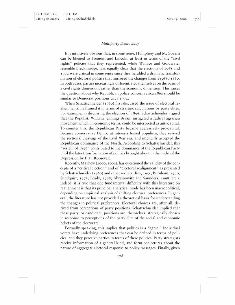
P1: GHM/FYC P2: GHM



It is intuitively obvious that, in some sense, Humphrey and McGoverncan be likened to Fremont and Lincoln, at least in terms of the “civilrights” policies that they represented, while Wallace and Goldwaterresemble Breckinridge. It is equally clear that the elections of 1968 and1972 were critical in some sense since they heralded a dramatic transfor-mation of electoral politics that mirrored the changes from 1856 to 1860.In both cases, parties increasingly differentiated themselves on the basis ofa civil rights dimension, rather than the economic dimension. This raisesthe question about why Republican policy concerns circa 1860 should besimilar to Democrat positions circa 1972.

When Schattschneider (1960) first discussed the issue of electoral re-alignments, he framed it in terms of strategic calculations by party elites.For example, in discussing the election of 1896, Schattschneider arguedthat the Populist, William Jennings Bryan, instigated a radical agrarianmovement which, in economic terms, could be interpreted as anti-capital.To counter this, the Republican Party became aggressively pro-capital.Because conservative Democrat interests feared populism, they revivedthe sectional cleavage of the Civil War era, and implicitly accepted theRepublican dominance of the North. According to Schattschneider, this“system of 1896” contributed to the dominance of the Republican Partyuntil the later transformation of politics brought about in the midst of theDepression by F. D. Roosevelt.

Recently, Mayhew (2000, 2002), has questioned the validity of the con-cepts of a “critical election” and of “electoral realignment” as presentedby Schattschneider (1960) and other writers (Key, 1955; Burnham, 1970;Sundquist, 1973; Brady, 1988; Abramowitz and Saunders, 1998; etc.).Indeed, it is true that one fundamental difficulty with this literature onrealignment is that its principal analytical mode has been macropolitical,depending on empirical analysis of shifting electoral preferences. In gen-eral, the literature has not provided a theoretical basis for understandingthe changes in political preferences. Electoral choices are, after all, de-rived from perceptions of party positions. Schattschneider implied thatthese party, or candidate, positions are, themselves, strategically chosenin response to perceptions of the party elite of the social and economicbeliefs of the electorate.

Formally speaking, this implies that politics is a “game.” Individualvoters have underlying preferences that can be defined in terms of poli-cies, and they perceive parties in terms of these policies. Party strategistsreceive information of a general kind, and form conjectures about thenature of aggregate electoral response to policy messages. Finally, given

178

P1: GHM/FYC P2: GHM



the utilities that strategists have concerning the importance of policy, andof electoral success, they advise their candidates how best to construct“utility maximizing” strategies for the candidates.

In the previous chapters of this book we have proposed that the “game”takes place in a policy space X, say, which is used to characterize individualvoter preferences. Each candidate j offers a policy position z j to theelectorate, chosen so as to maximize the candidate’s utility. Typically,this utility is a function of the “expected” vote share of the candidate. Itis also usually assumed that all candidates have similar utilities, in thateach one prefers to win. While there are many variants of this model, theconclusion asserted by the mean voter theorem, for example, is that allcandidates will adopt identical, or almost identical, policy positions in asmall domain of the policy space, centrally located with respect to thedistribution of voter-preferred points.

Any such formal model has little to contribute to an interpretation ofcritical elections or of electoral realignment. From the point of view ofthis literature, change can only come about through the transformationof electoral preferences by some exogenous shock. Even allowing for suchshocks, the divergence of party positions observed by Schattschneider canonly occur if perceptions of party strategists are radically different. Thisseems implausible.

In this chapter, we develop the model proposed in Chapter 7, in whichrational political candidates attempt to balance the need for resourceswith the need to take winning policy positions. Voters choose amongcandidates for both policy and nonpolicy reasons. The policy motivationsof voters pull candidates toward the center. However, centrist policies dolittle to earn the support of party activists, who are more ideologicallyextreme than the median voter, and who supply vital electoral resources.Candidates realize that the resources obtained from party activists makethem more attractive, independent of policy positions. This implies thatcandidates must balance the attractiveness of activists’ resources againstthe centrist tug of voters.

During most elections, there is a stable pattern of partisan cleavagesand alliances. In such an environment, candidates can adopt equilibriumvote-maximizing positions that allow them to appeal to one set of partisanactivists or another. But in certain critical elections, candidates realize thatthey can improve their electoral prospects by appealing to party activistson a new ideological dimension of politics. In the next section, we presenta sketch of the possible repositioning of presidential candidates in thecritical elections of 1860, 1896, 1932, and 1964–1968. We then develop

179

P1: GHM/FYC P2: GHM



an overview of the model to focus on the nature of activists’ choices. Inthe final two sections, we draw some further inferences with a view toproviding a deeper understanding of recent political alignments.

8.2 a brief political history, 1860–2000

Before introducing the model, it will be useful to offer schematic repre-sentations of the “critical elections” between 1860 and 1968 in order toillustrate what it is we hope to explain.

For Schattschneider, the 1896 election was based on an attack by Bryanagainst the sectional cleavage of the Civil War and the Reconstruction.It is therefore consistent with this argument that the contest between theRepublican, McKinley, and the Populist Democrat, Bryan, was character-ized by policy differences on a “capital” dimension. It is also convenientto refer to this dimension as an “economic” dimension. McKinley clearlyfavoured pro-business policies, while Bryan made a case for soft-money(bimetallism) and easy credit, both attractive to hard-pressed agrariangroups of the time. The sectional conflict of the Civil War era had ob-viously been over civil rights, so we can describe this earlier conflict interms of a “social” dimension. Another way of characterizing this dimen-sion is in terms of labour, since policies that restricted the civil rights ofsouthern blacks had significant consequences for the utilization of labour.To give a schematic representation of the election of 1860, we may thussituate Lincoln and Breckinridge in opposition on the social dimension,as in Figure 8.1. The Whig, Bell, may be interpreted as standing for thecommercial interests, particularly of the northeast. In contrast, Douglasrepresented the agrarian interests of the West, and his support came pri-marily from states such as Iowa, Ohio, Indiana, Illinois, and so forth.

With two distinct dimensions and four candidates, it is immediately ob-vious that the policy space could be divided into four quadrants. Voterswho had conservative preferences on both social and economic axes wemay simply term Conservatives. In the 1860 election, such voters wouldhave commercial interests and be pro-slavery. On the other hand, vot-ers with commercial interests, but who felt strongly that slavery shouldbe restricted we call Cosmopolitans. Voters opposed to both slavery andcommercial interests, we call Liberals. (This term is clearly something of amisnomer in 1860 since such voters would, at the time, probably be “freesoil” farmers in states such as Illinois, etc.). Agrarian, anticommercialinterests who were conservative on the social axis, we term Populists. For

180

P1: GHM/FYC P2: GHM



Republicans

Western Democrats

Liberal

Liberal

D: Liberals

A: Populists

C: Cosmopolitans

B: Conservatives

LINCOLN, 40%

DOUGLAS, 29% Whigs

BELL, 13%Conservative

Southern Democrats

BRECKINRIDGE, 18%

Conservative

ECONOMICDIMENSION

SOCIALDIMENSION

Figure 8.1. A schematic representation of the election of 1860 in a two-dimensional policyspace.

convenience, we denote these four quadrants as A (Populists), B (Conser-vatives), C (Cosmopolitans), and D (Liberals).

The boundaries in Figure 8.1 indicate the division of the electorate intothe supporters of the four presidential candidates in 1860. Figure 8.1 isintended to imply that each of the candidates in 1860 had to put together acoalition of divergent interests. Prior to 1852, the social or labour dimen-sion played a relatively unimportant role, at least in presidential elections.How and why this dimension came into prominence in 1856 has been dis-cussed at length elsewhere, using notions from social choice theory (Riker,1982; Weingast, 1998; Schofield, 2006a). It is our contention that the eco-nomic and social dimensions are always relevant to some degree in U.S.political history. However, at various times, one or the other may becomeless important, for reasons we shall explore. After the Civil War, and thedisappearance of the Whig Party (and of the distinct Western Democratfaction, represented by Douglas), political conflict between Republicansand Democrats focused on the social axis, as illustrated in Figure 8.2.

The horizontal “partisan cleavage line” is intended to separate theRepublican and Democrat voters immediately after the Civil War. It is

181

P1: GHM/FYC P2: GHM



BRYAN

Populists

ECONOMICDIMENSION

Conservatives

Conservative

Partisan cleavageline, 1896

Partisan cleavage line,Civil War to 1896

McKINLEY

ReconstructionRepublicans

ReconstructionDemocrats

SOCIALDIMENSION

Conservative

Liberals

Liberal

Liberal A B

CD

Cosmopolitans

Figure 8.2. Policy shifts by the Republican and Democratic Party candidates, 1860–1896.

consistent with Schattschneider’s interpretation of the election of 1896

that McKinley adopted a much more pro-business, or conservative, posi-tion on the economic axis, while Bryan took up a policy position in thepopulist quadrant (A). The 1896 partisan cleavage line in Figure 8.2 isused to distinguish between Republican and Populist Democrat voters.Figure 8.2 makes it intuitively clear why Bryan could not win the elec-tion. Moreover, support for conservative economic policies would lead toRepublican predominance. As Schattschneider (1960: 85) observed, “theDemocrat party carried only about an average of two states (outside ofsouthern and border states) between 1896 and 1932.” The increasing “de-gree of competition” between Democrat and Republican parties in 1932

can be represented by the positioning of F. D. Roosevelt and Hoover nearthe economic axis, as in Figure 8.3.

Note that the successful Roosevelt coalition comprised what we havecalled Populists and Liberals opposed to Conservatives and Cosmoplitans.

182

P1: GHM/FYC P2: GHM



Liberal

ECONOMICDIMENSION

PopulistDemocrats

Partisan cleavage line1924

Figure 8.3. Policy shifts by the Democratic Party circa 1932.

The standard formal model (Downs, 1957) has tended to generalize fromthe location of party positions in the period from 1932 to 1960 and toinfer that political competition is primarily based on the economic axis,and involves the coalition {A,D} against {B,C}. However, as Carminesand Stimson (1989) have analyzed in great detail, “race” (or “policy”on the social dimension) has become increasingly important since about1960. Indeed, they present data to suggest that Republicans in the Senatetended to vote in a more liberal fashion on racial issues than Democratsprior to 1965.

Although L. B. Johnson may have had many of the characteristics ofa Southern Democrat while he was Senate leader, he introduced, whilePresident, the major policy transformation of the Great Society. Figure 8.4presents a plausible policy position for Johnson in 1964, as well as pres-idential candidate positions for the period 1964 to 1980. The candidatepositions for the elections of 1968 and 1976 are compatible with the em-pirical work of Poole and Rosenthal (1984: Figs 1, 3), while the positions

183

P1: GHM/FYC P2: GHM



Liberal

Liberals

Liberal Conservative

Cosmopolitans

Conservatives

Conservative

SOCIALDIMENSION

HUMPHREY (1968)

CARTER(1976, 1980)

ANDERSON(1980)

JOHNSON(1964)

Domain ofCleavagelines

NIXON (1968)

FORD (1976)

REAGAN (1980)

GOLDWATER(1964)

WALLACE (1968)

Populists

ECONOMICDIMENSION

Figure 8.4. Estimated presidential candidate positions, 1964–1980.

for the elections of 1964 and 1980 are based on our analyses discussedbelow.

A number of comments are necessary to understand the significance ofthis figure. As in the previous two figures, a partisan cleavage line can bedrawn in the policy space for each election, determined by the positions ofthe two principal presidential candidates. What we denote as the “Domainof Cleavage lines” in Figure 8.4 includes these partisan cleavage lines forthe various elections. As our analysis (presented in Figure 8.5 below)suggests, the cleavage line for the 1964 election would fall below and tothe right of the origin. Since the origin is at the mean of voter bliss points,this is meant to represent Johnson’s successful candidacy for President.

The standard spatial model of candidate positioning implies that at-tempts by candidates to maximize votes draws them into the electoralcenter. It is apparent, however, that the estimates of candidate positions,presented in Figure 8.4, contradict this inference. Indeed, the positioning

184

P1: GHM/FYC P2: GHM



of Republican and Democrat candidates in Figure 8.4 suggests that vot-ers who can be described as Cosmopolitan (with preferences in the policydomain C) or Populists (in domain A) may find it difficult to choose be-tween the candidates.

In the next section, we examine the standard spatial model to determinethe basis for this inference, and then consider in somewhat more detailhow empirical analysis suggests how the standard spatial model may beadapted to better account for candidate behavior. The principal goal ofour modified activist voter model of elections is to provide the foundationfor a theory of dynamic electoral change that can provide a formal accountof the inferred transformation or “rotation” in the policy space presentedin Figures 8.1 through 8.4.

8.3 models of voting and candidate strategy

As we have discussed in the previous chapters, the formal model of votingassumes that voter utility is given by the expression

ui (xi , z) = (ui1(xi , z1), . . . , uip(xi , zp)) ∈ Rp. (8.1)

Here, z = (z1, . . . , zp) is the vector of strategies of the set P of politicalagents (candidates, parties, etc.). The point z j is the position of candidatej in the space X. Previously we assumed that

ui j (xi , z j ) = λ j − Ai j (xi , z j ) + θTj ηi + ε j , (8.2)

where Ai j was the symmetric Euclidean metric and θTj ηi gave the effect of

the sociodemographic characteristics of voter i on vote probabilities.As we have seen, both the MNL and MNP models typically provide an

excellent account of voter choice. For example, the MNL two-dimensionalvoter model of Poole and Rosenthal (1984) for the 1968 and 1976 elec-tions had success rates for voter choice of over 60 percent. Their estimatesof the 1968 and 1976 candidate locations closely correspond to the posi-tions of candidates indicated in Figure 8.4. As Poole and Rosenthal (1984:287) suggest, “the second dimension captures the traditional identifica-tion of southern conservatives with the Democratic party.”

Our own analyses, presented in Figures 8.5 and 8.6, suggest that thesecond dimension is, in fact, a long-term factor in U.S. elections. Eachcircle in these figures represents the ideal point of a voter in a factorspace derived from the National Election Surveys of 1964 and 1980,respectively.

185

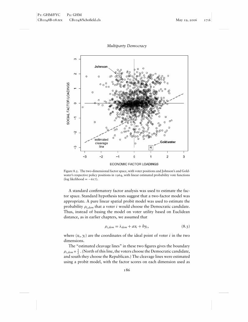
P1: GHM/FYC P2: GHM



Figure 8.5. The two-dimensional factor space, with voter positions and Johnson’s and Gold-water’s respective policy positions in 1964, with linear estimated probability vote functions(log likelihood = −617).

A standard confirmatory factor analysis was used to estimate the fac-tor space. Standard hypothesis tests suggest that a two-factor model wasappropriate. A pure linear spatial probit model was used to estimate theprobability ρi,dem that a voter i would choose the Democratic candidate.Thus, instead of basing the model on voter utility based on Euclideandistance, as in earlier chapters, we assumed that

ρi,dem = λdem + axi + byi , (8.3)

where (xi , yi ) are the coordinates of the ideal point of voter i in the twodimensions.

The “estimated cleavage lines” in these two figures gives the boundaryρi,dem = 1

2 . (North of this line, the voters choose the Democratic candidate,and south they choose the Republican.) The cleavage lines were estimatedusing a probit model, with the factor scores on each dimension used as

186

P1: GHM/FYC P2: GHM



Figure 8.6. The two-dimensional factor space, with voter positions and Carter’s and Rea-gan’s respective policy positions in 1980, with linear estimated probability vote functions(log likelihood = −372).

covariates. In both the 1964 and 1980 models, the estimated coefficientswere highly statistically significant (p < 0.001 in all cases). Both modelsclassify reasonably well; the McKelvey and Zavoina R2 for 1964 is 0.2000

and for 1980 is 0.465. (See Schofield, Miller and Martin, 2003, for fur-ther details.) Given the estimated probabilities, it is possible to infer thelocation of the two candidates. For example, for 1964, the symbol R isused to indicate our estimation of the position of Goldwater and D that ofJohnson. Comparing the results for 1964 and 1980 suggests that Carterwas just as “liberal” on economic issues as was Johnson, but slightly moreliberal on social issues. Notice that in 1964, the cleavage line ρi,dem = 1

2passes “south” of the origin, so that a clear majority of the voter sampleis assigned a probability greater than 1

2 of voting for Johnson. In contrast,in 1980, the cleavage line passes “north” of the origin, giving Reagan theadvantage.

187

P1: GHM/FYC P2: GHM



In 1964, the total electoral variance on the two axes was 1.28, while in1980 the variance was very similar at 1.365. Since the linear probabilitymodel is different from the one used in our previous analyses, we can-not use the convergence coefficient directly. In terms of the linear probitmodel, it is evident that Goldwater in 1964 and Carter in 1980 had lowerexogenous valences than their respective competitors. The above analysessuggest that all candidates were indeed positioned some distance from theelectoral origin.

Figures 8.5 and 8.6 buttress the remark made by Poole and Rosenthal(1984: 288) that their analysis “is at variance with simple spatial the-ories which hold that the candidates should converge to a point in thecenter of the [electoral] distribution” (namely, the origin in Figures 8.5and 8.6). Poole and Rosenthal suggest that this “party stability,” of diver-gent candidate locations, is the result of the need of candidates to appealto a support group to be nominated. Our earlier results suggest that thedivergent positions were consistent with vote maximization.

To see this, note that in their estimation of the vote function for 1968,the intercept, or valence λ for Humphrey and Nixon was 3.416, whilefor Wallace, it was 7.515. Moreover, the coefficient β was 5.260 forHumphrey and Nixon, but 7.842 for Wallace. In other words, the un-derlying valence, or innate attractiveness of Wallace was high, but votersupport dropped rapidly as the distance between the voter ideal point andthe Wallace position increased. In their analysis of the 1980 election, the β

coefficient for the third independent, National Union candidate, John An-derson, was 1.541. Anderson took only 6.6 percent of the national vote,and this is reflected in his estimated λ coefficient of −0.19, in contrast toλ = 3.907 for Carter and Reagan.

We now develop the model proposed in Chapter 7, where valence com-prises two components. For candidate j , there is an “innate” or exoge-nous valence whose distribution is characterized by the stochastic errorterm ε j. As before, the expectation of the valence term for candidate j isidentified with the average valence λ j , of j in the electorate. The secondcomponent, μ j , is affected by the money and time that activists makeavailable to candidate j . Essentially, this means that this second valencecomponent μ j is a function of the policy choices of candidates. We canignore the exogenous valence terms since they have been examined above.Concentrating on activist valence gives the following expression for voterutility:

ui j (xi , z j ) = μ j (z j ) − Ai j (xi , z j ) + ε j. (8.4)

188

P1: GHM/FYC P2: GHM



For convenience, in the discussion below we refer to the effect of candi-date strategies on the expected vote-share function E j , through change inμ j (z j ), as the valence component of the vote. Change in E j through theeffect on the policy distance measure Ai j (xi , z j ) we refer to as the nonva-lence, or policy component. We discuss this “activist” model in the nextsection. One important modification of the pure spatial model that wemake is that the salience of different policy dimensions varies among theelectorate. More precisely, we assume that

Ai j (xi , z j ) = ||xi − z j ||2i . (8.5)

Here, || · · · ||i is an “ellipsoidal” norm giving a metric whose coefficientsdepend on xi . We make this assumption clearer in the following section,where we assume that activists, motivated primarily by one policy di-mension or the other, may choose to donate resources that increase theircandidate’s valence. We argue that it is the candidate’s attempt to positionhimself with respect to different types of activists that accounts for thepartisan realignment.

8.4 a joint model of activists and voters

We adapt a model of activist support first offered by Aldrich (1983a,b)and introduced in the previous chapter.

Essentially the model is a dynamic one based on the willingness of vot-ers to provide support to a candidate. Given current candidate strategiesz let

C(z) = (C1(z), . . . ,Cp(z)) (8.6)

be the current level of support to the various candidates. The candidatesdeploy their resources, via television, and other media, and this has aneffect on the vector μ(z) = (μ1(z1), . . . , μp(zp)) of candidate-dependentvalences. We assume that each μ j is in fact a function of Cj (z j ).

At this point, a voter i may choose to add his own contribution ci j tocandidate j as long as

ci j < μ j (z j ) − Ai j (xi , z j ) + ε j. (8.7)

The total contributions to candidate j is then �ci j . Aldrich consideredan equilibrium of this dynamic process between two candidates, 1 and2, where the candidate’s position, z j , was defined to be the mean of theideal points of all activists who supported this candidate. The existence

189

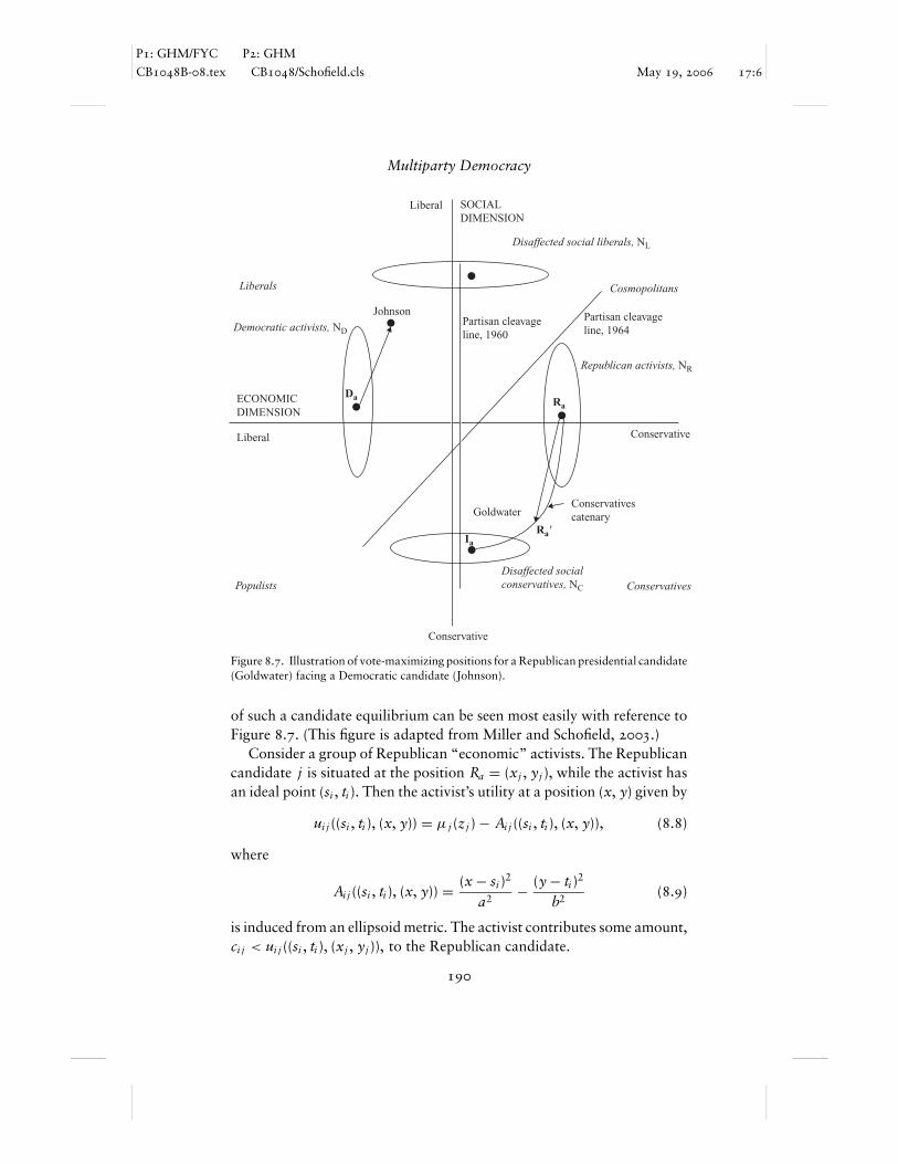
P1: GHM/FYC P2: GHM



Liberals

Liberal

Johnson

SOCIALDIMENSION

Disaffected social liberals, NL

Cosmopolitans

Republican activists, NR

Conservative

Conservatives

Conservative

Partisan cleavageline, 1960

Partisan cleavageline, 1964Democratic activists, ND

ECONOMICDIMENSION

Liberal

Da Ra

Goldwater

Ia

Ra'

Conservativescatenary

PopulistsDisaffected socialconservatives, NC

Figure 8.7. Illustration of vote-maximizing positions for a Republican presidential candidate(Goldwater) facing a Democratic candidate (Johnson).

of such a candidate equilibrium can be seen most easily with reference toFigure 8.7. (This figure is adapted from Miller and Schofield, 2003.)

Consider a group of Republican “economic” activists. The Republicancandidate j is situated at the position Ra = (xj , yj ), while the activist hasan ideal point (si , ti ). Then the activist’s utility at a position (x, y) given by

ui j ((si , ti ), (x, y)) = μ j (z j ) − Ai j ((si , ti ), (x, y)), (8.8)

where

Ai j ((si , ti ), (x, y)) = (x − si )2

a2− (y − ti )2

b2(8.9)

is induced from an ellipsoid metric. The activist contributes some amount,ci j < ui j ((si , ti ), (xj , yj )), to the Republican candidate.

190

P1: GHM/FYC P2: GHM



Because this activist is most concerned about economic issues, it isnatural to assume that a < b. If the activist actually had an ideal point(si , ti ) = Ra , then his indifference curve would be given by the “ellipsoid”centered at Ra , say. Depending on various parameters, there will exista domain NR, say, in X, with the property that every voter whose idealpoint (si , ti ) belongs to NR is a contributor to the Republican candidate.For purposes of illustration, we may take NR to be represented by the“ellipsoid” of ideal points centered on Ra , as in Figure 8.7. It is natural toassume that there is an opposing Democratic candidate, whose positionis at Da , say, and an opposing set ND of Democratic activists whose idealpoints belong to a similar set but are centered on Da . Aldrich showed,essentially, that these conditions could be satisfied, such that Ra was givenby the mean point of the set NR, while Da was the mean of the set ND. Itis obvious that for such an activist equilibrium to exist, it is necessary thateach μ j , regarded as a function of campaign contributions, is concave (orhas diminishing returns) in contributions to candidate j . (A more refinedmodel could naturally include voter income.)

As Figure 8.7 indicates, a typical socially conservative voter wouldregard Democrat and Republican candidates as equally unattractive, andtend to be indifferent. Let us now suppose that such a voter, g, has blisspoint (sg, tg), say, near the position Ia , with utility function

ugj ((sg, tg), (x, y)) = μ j (z j ) −(

(x − sg)2

e2+ (y − tg)2

f 2

). (8.10)

Let NC be the set of such “disaffected” social conservatives who wouldbe willing to contribute to a candidate as long as this candidate adopteda policy position close to Ia = (xk, yk). We suggest that such social con-servatives regard social policy to be of greater significance and so e > fin this equation. Unlike Aldrich, we now suppose that the Republicancandidate adopts a position, not at the position Ra , but at some compro-mise position R′

a between Ra and Ia . It is easy to demonstrate that the“contact curve” between the point (si , ti ) and the point (sg, tg) is given bythe equation

(y − ti )(x − si )

= S(y − tg)(x − sg)

, (8.11)

where

S = b2

a2

e2

f 2. (8.12)

191

P1: GHM/FYC P2: GHM



This contract curve between Republican economic activists and disaf-fected social activists is labeled the “Conservatives catenary” in Figure 8.7.If the candidate moves on this catenary then the resulting number of ac-tivists will be of the order of qNR + (1 − q)NC, where q is some constant(<1) dependent on the position taken by the candidate. Because of theasymmetry involved, the total number of activists may increase, thus in-creasing overall contributions to the Republican candidate. Clearly, thereare plausible conditions under which μrep increases as a result of such amove, thus potentially increasing the vote share of the Republican candi-date.

Determination of existence of a candidate PNE in this modified modeldepends, as before, on continuity and concavity of the candidate utility(or vote-share) functions {Uj }. While each Uj will be a function of z,its dependence on z will be more complex than the simple relationshipimplicit in the model we have studied above. It is important to note thatthis proposed model involves differing voter utility functions. To preservecontinuity of voter response, it is necessary that the coefficients of voterpolicy loss vary continuously with the voter-preferred policy. With theseassumptions, candidate vote-share functions {Uj } will be continuous incandidate strategies. Concavity of the candidate utility functions and thusexistence of PNE will then follow from assumptions about the concavityof the activist valence functions. It is worth emphasizing that the greaterthe relative saliencies, b/a and e/ f , the greater will be S and thus, themore significant will be the attraction of using activist groups to enhanceelectoral support.

Chapter 3 has shown that LNE will generally exist, and will be locallyisolated, for almost all games of the kind considered here, as long as thegame is smooth. As we have seen in the chapter on Britain, this allows usto assume that equilibria do exist in these complex activist games.

Computation of LNE will generally depend on the factors we havespecified: the elasticity of response of the disaffected, potential activists,and the effect of contributions on the valence functions {μ j }. If the con-tribution term is very significant, then adopting a position to maximizecontributions is clearly rational. For example, let us use R and D to denotethe positions adopted by the two candidates (as in Figure 8.7). Then it is,in principle, possible to estimate the contributions and thus the valencefunction. As the results of Chapter 7 indicated, a move by either candidatetoward the origin will increase the nonvalence component of the electoralvote, but at the same time, decrease contributions, and thus decreasethe valence component of the vote. It is the optimal balance of valence

192

P1: GHM/FYC P2: GHM



and nonvalence vote components that is encapsulated in the notion ofLNE.

8.5 the logic of vote maximization

The simple probabilistic voter model suggests that it is relatively easyfor voters to identify attractive candidates, and for candidates to learnabout voter response (McKelvey and Ordeshook, 1985). For candidates,the use of opinion polls can be used to indicate how small changes inpolicy objectives should affect support. The earlier theories of Hinich(1977) and Enelow and Hinich (1984) mentioned in Chapter 3 arguedthat candidates will gain most electoral support at the centre. The factthat candidates do not act in this way suggests that these theories needserious revision. One extreme response is to propose that voter support isindependent of candidate declarations. As suggested before, this is equiv-alent to supposing that the spatial component of the model is irrelevant.Indeed, earlier sociological or psychological models (Berelson, Lazerfield,and McPhee, 1954; Campbell et al., 1960) essentially made this assump-tion. The sociological model regarded voter choice simply as a function of“party identification.” It is clear enough that if one fundamental cleavageis dominant, and party candidates adopt fixed positions on this cleavage(as in Figure 8.7) then voters will find candidate choice relatively easy.Over a sequence of elections, it is plausible to believe that voters will tendto identify with one party or the other. From one election to another,voter saliencies will vary, and this will affect activist support, and thuscandidate vote shares. It is this phenomenon that Aldrich’s activist modelanalyzed (Aldrich, 1983a,b; Aldrich and McGinnis, 1989; Aldrich, 1995).If we are correct in our interpretation of U.S. electoral politics, then anoptimal response by a Democrat candidate to the socially conservativeRepublican position is to adopt a more economically centrist position. Itis possible that Clinton’s successes in 1992 and 1996 were a results ofsuch a strategy.

Over the years there will be slow transformations in the principal elec-toral cleavage, and it is the change from one cleavage, or electorally per-ceived dimension, to another that constitutes an electoral “realignment.”

The beginning of the last transformation of the principal cleavage inU.S. politics from an economic dimension to a social, or civil rights, dimen-sion is generally understood to have been triggered by the Civil Rights Actof 1964 (Huckfeldt and Kohfeld, 1989; Edsall and Edsall, 1991; Mann,1996). This political event eventually brought about the electoral shifts

193

P1: GHM/FYC P2: GHM



that we described earlier. The evidence suggests that the degree of partyidentification dropped from 1964 to 1980 (from about 35 percent of theelectorate to 20 percent: see Clarke and Stewart, 1998). During the pe-riod from 1960 to 1972, attitudes of Democrat and Republican activistsbecame increasingly polarized over civil rights issues (Carmines and Stim-son, 1989). There is therefore no doubt that both voter perceptions andactivist attitudes began to change rapidly in the 1960s. The model pre-sented in the previous section suggests that these changes were due tostrategic calculations on the part of candidates. To amplify this inference,let us consider how such calculations can be made.

Unlike candidate choice in the simple spatial model, strategic calcula-tion in the proposed activist model is dependent on uncertain outcomes.Consider the strategy of L. B. Johnson to push through the Civil RightsAct of 1964. Clearly, it appealed to those voters designated “disaffectedsocial liberals” in Figure 8.7. The argument presented above suggests thatthe total number of Democrat activists could increase as a consequence ofthis policy initiative. The resources made available could, moreover, in-crease Johnson’s overall valence. At the same time, voters, particularly inthe Southern states, who traditionally identified with the Democrat party,would suffer a utility loss. Such disaffected social conservatives wouldthen more readily switch to the Republican party. However, the tradeoffbetween the valence and policy components of voter response is intrinsi-cally difficult to make. For L. B. Johnson, the calculation may well havebeen that the Democrat coalition of southern social conservatives andeconomic liberals was unstable. A second, but contradictory, possibility,apparent from 1957 onwards, was that the Republican Party could alsomove to attract social liberals and create a winning coalition. The actionsundertaken by Johnson, first as leader of the Senate in the late 1950s, andthen as President after J. F. Kennedy’s assassination in 1963, all suggestthat he was extremely shrewd in estimating electoral and congressionalsupport, but also capable of extreme risktaking. In 1957, for example,he persuaded the Southern Democratic senators not to deploy their tradi-tional filibuster, but to accept the Voting Rights Bill (Caro, 2002). Indeed,Johnson’s maneuvers in the Senate can be characterized as “heresthetic”(to use the term invented by Riker [1982]).

After Kennedy was elected President in 1960 (by a very narrow mar-gin of victory against Nixon), he delayed sending a Civil Rights Bill toCongress, precisely because of the possible effect on the South. To pushthrough the Civil Rights Act in July 1964, Johnson effectively created, withHubert Humphrey’s support, an unstable coalition of liberal Northern

194

P1: GHM/FYC P2: GHM



Democrats and moderate Republicans, with sufficient votes in the Senateto effect “cloture,” to block the southern Democratic filibusters (Branch,1998). This was the first time since Reconstruction that the southern vetowas overwhelmed. The danger for Johnson in the election of 1964 wasthat a Republican candidate could make use of the fact of RepublicanParty support for civil rights to attract disaffected social liberals. Tradi-tional Republican Party activists were thus in an electoral dilemma, butresolved it by choosing the southern social conservative, Goldwater.

Once L. B. Johnson initiated the policy transformation, the strategiccalculation of Republican candidates, whether Nixon, Ford, Reagan, orBush, became much easier. The knowledge of the existence of a set ofdisaffected social conservatives meant that such voters would appear in-creasingly attractive to Republican candidates. This in turn created anelectoral dilemma for Democrats, as they attempted to maintain supportof both economic and social liberals. As economic competition decreasedin importance and class became less relevant as an indicator of voterchoice, activist support for Democrat candidates from the remnant of theNew Deal coalition would fall. One possible response for a Democratwould be to seek new potential activists among the Cosmopolitans—theeconomically conservative social liberals. Obviously, this would createconflict within the Democrat Party elite. A natural response by the Re-publican Party was to move their policy choices into quadrant A, thePopulist domain. President G. W. Bush’s initiatives in 2002, over pro-tection for the steel industry and farm subsidies, indicate that this could,indeed, be his strategy. Support for G. W. Bush in the 2004 election wouldseem to support this hypothesis. (See also Fiorina, 2005.)

We suggest that the initial policy move by Johnson in 1964 had a ba-sis in rational electoral calculation. Obviously the model proposed hereignores the element of attitude to risk, and this clearly must have been rele-vant to Johnson’s motivation, so this feature is worth adding to the model.At a general level it does appear that the resulting moves and counter-moves by Democrat and Republican candidates were in local equilibriumat each election, while the equilibria themselves appear to have slowlychanged over the last forty years. We could say that the entire process ofpolitical realignment over this period was in “dynamic equilibrium.”

8.6 dynamic local equilibria

Under plurality rule, or winner-takes-all electoral methods, it is obviousthat presidential candidates, if they hope to win, must attempt to create

195

P1: GHM/FYC P2: GHM



majority coalitions of disparate interests (Schlesinger, 1994). The histori-cal record suggests that stable equilibria can occur, but these will be basedon one or the other of the two principal cleavages—economic and social—that characterize beliefs in the society. Any such equilibrium, by definition,will create two groups of disaffected, and opposed, voters. Either one ofthese groups of voters can become a political force once they realize theirpotential. This depends, of course, on their ability to successfully signalto a candidate, such as L. B. Johnson, that they would be willing to con-tribute time and money. Although we have suggested that an equilibriumwill exist in this activist-voter model, we have not attempted an analysisof the complexities of the signaling game between possible presidentialcandidates and potential activists.

It should also be evident, from the structure of the activist model pre-sented here, that the willingness of voters to become activists depend onthe salience ratios (denoted by b/a and e/ f for the economically and so-cially concerned voters, respectively). These ratios may change within theelectorate as a result of exogenous shocks. In turn, this will affect the ac-tivist response to candidate positions and thus the positional valences ofthe candidates. The standard spatial model has principally depended onusing data based on voter-preferred policies to estimate electoral support.To estimate the more complex activist model proposed here, it would benecessary to explore the variation of cleavage saliencies within the elec-torate.

Although we still view the political process as a “game” involvingrational utility–maximizing voters and candidates, we suggest that thisgame is much more complex than previous models have suggested. Webelieve that the model proposed here can be developed so as to offer amore empirically relevant theory of electoral dynamics.

A task that still remains is to develop a macropolitical account of thelong run transformations that can be observed in U.S. politics. We canonly offer a very tentative outline of such a theory at present. We havesuggested above that these electoral changes are based on new configura-tions of “factor” coalitions, where factor refers to the classic dimensionsof capital, labor, and land power. In the 1896 election, the twenty-twostates that voted for the Republican, McKinley, all had significant indus-trial working class populations. Because of the growth of the economicpower of the United States, there existed a natural expansionist coalitionbased on capital and industrial labor (Rogowski, 1989). The hard-moneypolicy of the Republicans naturally affected the agrarian interests (whotended to be indebted), as argued by Bardo and Rockoff (1996). This

196

P1: GHM/FYC P2: GHM



is an old theme in U.S. politics (Beard, 1913). The twenty-three statesthat voted for the Populist-Democrat, Bryan, were all basically agrarianbut lacked sufficient population and electoral college votes to upset thecapital–labor coalition.

In the 1930s, economic decline broke the capital–industrial labor coali-tion. By the 1960s, the Democrat coalition comprised half of Bryan’ssouthern Populist states and half of McKinley’s commercial Republicancoalition. By the 2000 election, the transformation was complete. Theremainder of Bryan’s coalition became Republican, and the remainder ofMcKinley’s became Democrat. The decline of agriculture and the growthof modern industries in the southern and western states gave them the pop-ulation and electoral college votes just sufficient for a Republican presi-dential victory. Clearly, the knife-edge result of the 2000 election indicatesthat voters in states such as Wisconsin, Michigan, Minnesota, Pennsyl-vania, and Iowa could be persuaded by G. W. Bush’s populist strategiesto join the Republican activist coalition. Such continuing transformationmaintains the dynamic equilibrium of U.S. politics.

8.7 appendices

(i) The Civil Rights Act.Date: 02 JUL 64

88th Congress, H. R. 7152

An ActTo enforce the constitutional right to vote, to confer jurisdiction upon

the district courts of the United States to provide injunctive relief againstdiscrimination in public accommodations, to authorize the Attorney Gen-eral to institute suits to protect constitutional rights in public facilities andpublic education, to extend the Commission on Civil Rights, to preventdiscrimination in federally assisted programs, to establish a Commissionon Equal Employment Opportunity, and for other purposes.

Be it enacted by the Senate and House of Representatives of the UnitedStates of America in Congress assembled, That this Act may be cited asthe “Civil Rights Act of 1964.”

(ii) Amendment XIV of the Constitution.Section 1. All persons born or naturalized in the United States and

subject to the jurisdiction thereof, are citizens of the United States andof the State wherein they reside. No State shall make or enforce any lawwhich shall abridge the privileges or immunities of citizens of the UnitedStates; nor shall any State deprive any person of life, liberty, or property,

197

P1: GHM/FYC P2: GHM



without due process of law; nor deny to any person within its jurisdictionthe equal protection of the laws.

Section 2. Representatives shall be apportioned among the sev-eral States according to their respective numbers, counting the wholenumber of persons in each State, excluding Indians not taxed. But whenthe right to vote at any election for the choice of electors for Presidentand Vice President of the United States, Representatives in Congress, theExecutive and Judicial officers of a State, or the members of the Legisla-ture thereof, is denied to any of the male inhabitants of such State, beingtwenty-one years of age, and citizens of the United States, or in any wayabridged, except for participation in rebellion, or other crime, the basis ofrepresentation therein shall be reduced in the proportion which the num-ber of such male citizens shall bear to the whole number of male citizenstwenty-one years of age in such State.

Section 3. No person shall be a Senator or Representative in Congress,or elector of President and Vice President, or hold any office, civil or mili-tary, under the United States, or under any State, who, having previouslytaken an oath, as a member of Congress, or as an officer of the UnitedStates, or as a member of any State legislature, or as an executive or judi-cial officer of any State, to support the Constitution of the United States,shall have engaged in insurrection or rebellion against the same, or givenaid or comfort to the enemies thereof. But Congress may by a vote oftwo-thirds of each House, remove such disability.

Section 4. The validity of the public debt of the United States, au-thorized by law, including debts incurred for payment of pensions andbounties for services in suppressing insurrection or rebellion, shall notbe questioned. But neither the United States nor any State shall assumeor pay any debt or obligation incurred in aid of insurrection or rebellionagainst the United States, or any claim for the loss or emancipation of anyslave; but all such debts, obligations and claims shall be held illegal andvoid.

Section 5. The Congress shall have power to enforce, by appropriatelegislation, the provisions of this article.

The Fourteenth Amendment of the Constitution was passed by theHouse and Senate on the 8th of June and the 13th of June, 1866.

198

P1: FBQ


9

Concluding Remarks

9.1 assessment of the model

We briefly conclude with an assessment of the model presented in thisbook, together with some remarks on how the work can be extended.

The essence of democracy is that voters respond to the past acts andpromises of party leaders. It has been traditional to use manifestos asmeasures of promises, and to gauge the distance between the preferredpolicy of the voter and the promise of the party leader as the “disutility”of the voter. In addition, of course, the voter may not trust the party leader.Valence is one very simple way to model the judgment of the voter aboutthe degree to which the party leader can be trusted. This addition to thestandard spatial model of voting changes one of the principal results of themodel, namely the mean voter theorem. As the main theorem of Chapter3 shows, it is no longer necessarily the case that all parties will convergeto an electoral center. Instead, each election will be characterized by aconvergence coefficient. Empirical analysis associated with the electioncan be used to give a list of valence coefficients for each of the partyleaders. If the valences are similar, then the convergence coefficient willbe low, and symmetry will induce all parties to converge to the center.

The formal model shows that this convergence coefficient is an in-creasing function of the valence differences, the electoral variance, andthe spatial parameter. Moreover, with many parties with differing va-lences, the coefficient will tend to be high. When the coefficient exceedsthe dimension of the policy space, then the lowest-valence party will va-cate the electoral mean in order to increase its vote share. One way tointerpret this finding is that in such a circumstance the low-valence partycan guarantee itself more votes by seeking the electoral periphery ratherthan by competing directly with high-valence parties.

199

P1: FBQ



It is often thought that radical parties gain few votes because they areradical. The theory presented here suggests that when policy is important,and when electoral preferences are heterogeneous, then only parties thatare generally trusted by the electorate can approach the electoral center.The movement away from the electoral center by a low-valence party willbe determined by the principal component of the electoral distribution.Asymmetry in the nature of electoral preferences will result in a principalelectoral dimension, and it is this dimension that is the “eigenspace” fora low-valence party. Once the lowest-valence party leaves the electoralmean, then so will others. In general, all parties will adopt positions on theprincipal component of the voter distribution, but higher-valence partieswill choose positions nearer the mean.

This stochastic spatial model does not specify whether parties move upor down the principal electoral component. The theory assumes that thefinal vector of party positions is in “local equilibrium.” Given a systemof electoral parameters, there may be multiple local equilibria. Nonethe-less, it is plausible that the particular local equilibrium that occurs is “pathdependent.” That is, the previous historical situation generates a set of po-litical niches wherin parties typically reside. Notice that the differing localequilibria may be associated with very different political configurations.It may also be the case that small changes in the electoral parameters candramatically transform the local political equilibrium, destroying politicalniches and leading to the creation of new parties and new niches.

9.2 proportional representation

When the electoral system is based on some form of proportional rep-resentation, it is generally impossible for one party to gain a majority.Because coalitions involve compromise over policy, rational party prin-cipals should nominate leaders for the party who are in a position tobargain effectively with other party leaders. For low-valence parties oc-cupying niches far from the electoral center, this motivation may cause theparty elite to consider party leaders who have preferred positions that areeven more radical than the vote-maximizing position. For high-valenceparties, whose niches are close to the electoral center, there is an addedcentripetal tendency. If the party can position itself centrally and gainenough seats to be dominant, then it can occupy the “structurally stablecore” position, which will allow it, under some circumstances, to con-trol government, and perhaps to construct a minority government. Small

200

P1: FBQ


Concluding Remarks

changes in electoral support can therefore make a big difference whethera party is dominant or not.

9.2.1 The Election of September 2005 in Germany

Though we have not considered a formal model of German elections, therecent election in Germany on September 18, 2005, can be used to illus-trate some of the logic of coalition. The CDU/CSU (Christian Democrats,under Merkel) took 35.2 percent of the popular vote (and 225 seats inthe 613-seat Bundestag). The SPD (Social Democrats, led by Schroeder)took 34.3 percent (and 222 seats) against 8.1 percent (and 51 seats) forthe Greens, 8.7 percent (and 54 seats) for the Left Party, including PDS(Party for Democratic Socialism), and 9.8 percent (with 61 seats) for theFDP (Free Democrats). The previous SPD–Green coalition had 47.1 per-cent of the vote but 306 seats out of 603 in the Bundestag (slightly morethan proportional because the PDS had failed to gain 5 percent of thevote). The CDU–CSU–FDP coalition thus had 286 seats (not a majority),while the SPD–Green coalition had 273 seats. Figure 9.1 suggests thatthe PDS lies on a separate axis (labelled East/West) from the other fourparties. In which case it is obvious that the PDS (mostly excommunistsfrom East Germany) would be crucial in creating a majority with eitherthe SPD–Green or the CDU–CSU–FDP coalition. It may be able to selecta coalition partner and effectively pivot in the coalition game. Notice thatthere are at least three very different coalitions that can come into being,and these together define the heart of the Bundestag, namely the convexhull of the party positions, as in Figure 9.1.

For multiparty polities in which there is no majority party, we haveargued that there are essentially two qualitatively different post-electiondecisive structures. One is where Parliament is characterized by a struc-turally stable core, or, in more traditional terms, a central dominant party.The second is one in which no such dominant core party emerges and thecore of the legislature is empty. In the case of a structurally stable core,the policy that Parliament is expected to implement is the policy positionof the dominant party. If the core is empty, the policy that Parliamentwill adopt is bound to shift constantly but remain within what we termedthe heart of Parliament. If Figure 9.1 gives an approximate estimate ofparty positions after the September 2005 election in Germany, then thereis obviously no core party. In the full theory of coalition formation pre-sented in Chapter 3, we suggest that, in the absense of a core, the cheapestminimal winning coalition will tend to form, where this term refers to the

201

P1: FBQ



Economic Axis

PDS: Party of DemocraticSocialism-Left Party 8.7%54 seats

Eas

t-W

est A

xis

Green Alliance 8.1%51 seats

Social DemocratsSPD 34.3%222 seats

FreeDemocratsFDP 9.8%61 seats

Christian DemocratsCDU/CSU 35.2%225 seats

Figure 9.1. Schematic representation of party positions in the Bundestag in Germany,September 2005.

“smallest average policy distance” between the coalition members. TheCDU-SPD coalition that finally formed in November, 2005, is an exampleof such a coalition.

9.2.2 Recent Changes in the Israel Knesset

We may also make some comments with regard to recent changes inIsrael. Figure 9.2 provides a schematic representation of the 2003 Knesset

202

P1: FBQ


Concluding Remarks

-2

-1.5

-1

-0.5

0

0.5

1

1.5

2

-2 -1 0 1 2

Labour, 21 Seats

Likud, 40 Seats

Shinui, 15 Seats

Meretz, 6 Seats


NRP, 6 Seats

Israel Beiteinu, 7 Seats


Heart

Arab

Merertz

Shas

Shinui

Likud

NRP

IsraelBeiteinu

Security

Religion

Labour

Figure 9.2. A schematic representation of the configuration of the Knesset in 2003.

based on the party positions estimated in Chapter 3 and seat allocationsgiven in Table 2.1. The figure shows Labour with 21 seats, after AmEhad, with 2 seats, joined Labour in 2003, while Likud has 40 seats afterbeing joined by Olim, with 2 seats. Although Barak, of Labour, becamePrime Minister in 1999, he was defeated by Ariel Sharon, of Likud, inthe election for prime minister in 2000. The set denoted the heart in thisfigure represents the coalition possibilities open to Sharon after 2003.

The figure can be used to understand the consequences after Sharonseemingly changed his policy on the security issue in August, 2005, bypulling out of the Gaza Strip. First, the Likud party reacted stronglyagainst this change in policy. In the first week of November, 2005, AmirPeretz, a union activist, and leader of Am Ehad, won the election forleader of the Labour Party. This event can be seen as an illustration ofthe argument in Chapters 7 and 8 above, where we suggest that a partythat fails to attract voters because of a low relative valence will eventuallybe controlled by party activists. From this perspective, the low valenceof Labour vis-a-vis Sharon was the reason the Labour members chosePeretz.

Many observers regarded the change in the leadership of Labour as acritical transformation in the political map of Israel. However, as Figure9.3 suggests, the shift to the left by Labour under Peretz had no effect

203

P1: FBQ



-2

-1.5

-1

-0.5

0

0.5

1

1.5

2

-2 -1 0 1 2

Labour, 21 Seats

Likud, 40 Seats

Shinui, 15 Seats

Meretz, 6 Seats


NRP, 6 Seats

Israel Beiteinu, 7 Seats


Heart

Arab

Merertz

Shas

Shinui

Likud

NRP

IsraelBeiteinu

Security

Religion

Labour

Figure 9.3. The configuration of the Knesset after Peretz becomes leader of Labour.

on the heart of the Knesset. According to our model, there would be noeffect on party bargaining.

However, the move by Labour did have indirect consequence. In ahighly publicized move, Sharon left the Likud Party and signaled a strongmove to the left by allying with Shimon Peres, the former leader of Labourand the author of the Oslo accords. Together these two, with a numberof other senior Labour Party members, formed the new party, Kadima(“Forward”). This move positioned Sharon at the origin of the electoralspace at (0,0) as shown in Figure 9.4. In Chapter 3 the simulations of elec-tions in Israel demonstrated that Likud was unable to “capture the core.”By moving Labour to the left, Peretz created the opportunity for Sharonto out-maneuver him. Sharon could strategically move to a position thatwould increase the probability that he would control the core. BecauseSharon’s own party members would not support him in this move, he hadto leave Likud and form Kadima.

However, Figure 9.4 suggests that the seat strengths were insufficientfor Sharon to actually conrol the core in 2005. Indeed, the heart is boundedby the three median lines drawn in the figure. Since these lines do notintersect, the core is empty. Note however, that the new configuration

204

P1: FBQ


Concluding Remarks

-2

-1

0

1

2

-2 -1 0 1 2

Kadima, 42 seats

Labour, 20 seats

Likud, 15 seats

Shinui, 2 seats

Meretz, 5 seats

Arab Parties, 10 seats

NRP, 5 seats

Israel Beiteinu, 5 seats

Shas,Yahadut, 16 seats

Arab

Meretz

Shas

Labour

Kadima

Shinui

Likud

NRP

Israel

Beiteinu

Security

Religion

Figure 9.4. The effect of the creation of Kadima by Ariel Sharon on the configuration of theKnesset.

of the heart suggests a possible government coalition of Kadima withsupporters from factions of either Likud or Labour.

In a less publicized move, Sharon took his political maneuvering a stepfurther, obtaining the support of Uriel Reichman, founder of the Shinuiparty, for Kadima. On the face of it, this move seemed hard to explain.Although Reichman is a notable figure in Israel (currently the Presidentof IDC, the largest and most successful private university in Israel), hehas never held an elected office. In fact, Sharon promised Reichman theposition of Minister of Education in a Kadima coalition government. Thepurpose of this contract is clear from Figure 9.5. By obtaining Reichman’ssupport, Sharon made a small move “south” in the policy space towardsthe structurally stable core. Indeed this position is very close to the positionpreviously held by the Labour Party, under the leadership of Rabin, at the1992 election in Israel.

Figure 9.5 gives our estimates of party positions at the March 28, 2006,election to the Knesset. Because of Sharon’s stroke in January, 2006, EhudOlmert had taken over as leader of Kadima. Although his valence was pre-sumably lower than that of Sharon, Kadima was still able to take 29 seats.Likud, together with religious parties, took 50 seats. One surprise of the

205

P1: FBQ



-2

-1

0

1

2

-2 -1 0 1 2

Arab

Meretz

Shas, Yahadut

Labour

Kadima

Pensioners

Likud

NRP

IsraelBeiteinu

Security

Religion

Kadima, 29 seats

Labour, 19 seats

Likud, 12 seats

Pensioners, 7 seats

Meretz, 5 seats

Arab Parties, 10 seats

NRP,9 seats

Israel Beiteinu, 11 seats

Shas,Yahadut, 18 seats

Figure 9.5. The configuration of the Knesset after the election of 28 March, 2006.

election was the appearance of a pensioners’ party with 7 seats. However,this had no effect on coalition bargaining. Because a coalition betweenLabour and the religious parties is infeasible, we can infer that Kadima islocated at the structurally stable core position (as indicated in Figure 9.5).It appears that Sharon’s change of policy has led to a fundamental trans-formation in the political configuration, from the D0-coalition structurethat had persisted since 1996, to a D1-structure associated with the newcore party, Kadima.

9.3 plurality rule

Under plurality rule (in Britain or the United States, for example), wefollow Miller and Schofield (2003) and suggest that coalition forma-tion principally takes place inside the party rather than outside. In theUnited States, for example, parties are coalitions of disparate intereststhat are maintained only by bargaining between opposed activist groups.For Britain, we have refined this model, and have examined the effecton the “exogenous” valence of the party leader on the bargain made be-tween the leader and the various activist support groups. Since exogenousvalence is intrinsic to the party leader, calculating the marginal effects of

206

P1: FBQ


Concluding Remarks

exogenous valence and activist valence allows us to conclude that increas-ing leader valence reduces the radical effect of activists.

Although the theory is most readily applied to the situation where thereare disciplined parties in the Parliament, it is also applicable to the morecomplex situation of weakly disciplined parties in the U.S. Congress, witha President able to implement a veto. For presidential elections, we arguethat the changing composition of activist support has generated a slowtransformation in the positions of the candidates for the two parties.We suggest that this is the cause of what is sometimes called politicalrealignment.

Although we have not examined the relationship between Presidentand Congress in the U.S. case, we might expect a core to exist (or at leasta restricted heart) when the presidential party controls both House andSenate. In this case, computation of the heart will depend on the particulardistribution of policy preferences in both houses of Congress as well asthe policies to which the President is committed.

9.4 theory and empirical evidence

The theory that we have presented in this volume came about becauseof the apparent empirical refutation of the generally accepted theories ofelections. In our earlier work with our collaborators on Britain, Israel, theNetherlands, the United States, and, later, Italy, we found no evidence ofa significant centripetal tendency to an electoral center. Initially, we didnot see the significance of the intercept or valence terms in the electoralmodels. The simulations that we performed for Israel, however, made itclear that these terms, though they appeared to be trivial, had the effect ofcompletely changing the nature of the equilibria. The “first-order theory”with exogenous valence that we developed gave quite a good approxima-tion to the major party positions in Israel. Moreover, the formal resultwas bolstered by the correspondence between the theoretical finding andthe simulation of the electoral model.

The “second-order theory” involving the “structurally stable core” andcoalition bargaining, gave us a qualitative explanation for the location ofpivotal parties, such as Shas in Israel, off the principal electoral axis.

The analysis of Italy and the Netherlands made it obvious that partyactivists should be brought into the electoral equation. The empirical workon Britain, based on the MP survey data, suggested that activists for eachparty would be quite heterogeneous, and this reinforced the inferencemade by Miller and Schofield (2003) that a party is itself a coalition.

207

P1: FBQ



This suggested the tradeoff between activist support and leader valence.The importance of activists in the U.S. party system, together with thechanging nature of the intraparty bargain then naturally led us to the ideaof the transformation of party candidate positions and the phenomenonof political realignment.

This “third-order theory” of activists is only sketched here, but webelieve it will prove a fertile source of ideas about party competition.

We hope that this nested set of theories will be used in the future toconstruct an empirically relevant theory of democracy.

208

P1: FBQ

CB1048B-ref.tex CB1048/Schofield.cls March 30, 2006 21:21

References

Abramowitz, A., and K. Saunders. 1998. “Ideological Realignment in the U.S.Electorate.” The Journal of Politics 60(4):634–652.

Adams, J. 1999a. “Multiparty Spatial Competition with Probabilistic Voting.”Public Choice 99:259–274.

Adams, J. 1999b. “Policy Divergence in Multicandidate Probabilistic Spatial Vot-ing.” Public Choice 100:103–122.

Adams, J. 2001. Party Competition and Responsible Party Government. Ann Ar-bor: University of Michigan Press.

Adams, J., and S. Merrill, III. 1999. “Modeling Party Strategies and Policy Repre-sentation in Multiparty Elections: Why are Strategies So Extreme?” AmericanJournal of Political Science 43:765–781.

Adams, J., S. Merrill, III, and B. Grofman. 2005. A Unified Theory of PartyCompetition. Cambridge: Cambridge University Press.

Aldrich, J. H. 1983a. “A Downsian Spatial Model with Party Activists.” AmericanPolitical Science Review 77(3):974–990.

Aldrich, J. H. 1983b. “A Spatial Model with Party Activists: Implications forElectoral Dynamics.” Public Choice 41:63–100.

Aldrich, J. H. 1995. Why Parties? Chicago: Chicago University Press.Aldrich, J. H., and M. McGinnis. 1989. “A Model of Party Constraints on Opti-

mal Candidate Positions.” Mathematical and Computer Modelling 12:437–450.Aldrich J. H., G. J. Miller, C. W. Ostrom Jr., and D. Rohde. 1986. American

Government. Boston: Houghton Mifflin.Alvarez, M., and J. Nagler. 1998. “When Politics and Models Collide: Estimating

Models of Multicandidate Elections.” American Journal of Political Science42:55–96.

Alvarez, M., J. Nagler, and S. Bowler. 2000. “Issues, Economics, and the Dynamicsof Multiparty Elections: The British 1987 General Election.” American PoliticalScience Review 94:131–150.

Ansolabehere, S., and J. Snyder. 2000. “Valence Politics and Equilibrium in SpatialElection Models.” Public Choice 103(2000):327–336.

Aragones, E., and T. Palfrey 2002. “Mixed Equilibrium in a Downsian Modelwith Favored Candidate.” Journal of Economic Theory 103:131–161.

209

P1: FBQ


References

Arian, A., and M. Shamir. 1990. The Election in Israel: 1988. Albany: SUNYPress.



Arrow, K. 1951. Social Choice and Individual Values. New Haven: Yale UniversityPress.

Austen-Smith, D., and J. S. Banks. 1988. “Elections, Coalitions and LegislativeOutcomes.” American Political Science Review 82:405–422.

Austen-Smith, D., and J. S. Banks. 1990. “Stable Portfolio Allocations.” AmericanPolitical Science Review 84:891–906.

Austen-Smith, D., and J. S. Banks. 1999. Positive Political Theory I: CollectivePreferences. Ann Arbor: University of Michigan Press.

Austen-Smith, D., and J. S. Banks. 2005. Positive Political Theory II: Strategy andStructure. Ann Arbor: University of Michigan Press.

Austen-Smith, D., and J. R. Wright. 1992. “Competitive Lobbying for a Legisla-tor’s Vote.” Social Choice and Welfare 19:229–257.

Axelrod, R. 1980. Conflict of Interest. Chicago: Markham.Banks, J. S. 1990. “A Model of Electoral Competition with Incomplete Informa-

tion.” Journal of Economic Theory 50:309–325.Banks, J. S. 1995.“Singularity Theory and Core Existence in the Spatial Model.”

Journal Mathematical Economy 24:523–536.Banks, J. S., and J. Duggan. 2000. “A Bargaining Model of Collective Choice.”

American Political Science Review 94:73–88.Banks, J. S., and J. Duggan. 2005. “The Theory of Probabilistic Voting in the

Spatial Model of Elections.” In D. Austen-Smith and J. Duggan [Eds.]. SocialChoice and Strategic Decisions. Heidelberg: Springer.

Banks, J., J. Duggan, and M. Le Breton. 2002. “Bounds for Mixed Strategy Equi-libria and the Spatial Model of Elections.” Journal of Economic Theory 103:88–105.

Bardo, M., and H. Rockoff. 1996. “The Gold Standard as a Good HousekeepingSeal of Approval.” The Journal of Economic History 56(2):389–428.

Barnett, W., M. Hinich, and N. Schofield [Eds.]. 1993. Political Economy: In-stitutions, Competition and Representation. New York: Cambridge UniversityPress.

Barnett, W., H. Moulin, M. Salles, and N. Schofield [Eds.]. 1995. Social Choice,Welfare and Ethics. New York: Cambridge University Press.

Baron, D. P., and J. A. Ferejohn. 1989. “Bargaining in Legislatures.” AmericanPolitical Science Review 83:1181–1206.

Bartolini, S., and R. D’Alimonte [Eds.]. 1995. Maggioritario non troppo. Bologna:Il Mulino.

Beard, C. 1913. An Economic Interpretation of the Constitution of the UnitedStates. New York: Macmillan.

Berelson, B. R., P. R. Lazarfield, and W. N. McPhee. 1954. Voting: A Study ofOpinion Formation in a Presidential Campaign. Chicago, IL: Chicago Univer-sity Press.

210

P1: FBQ


References

Bianco, W. T., I. Jeliazkov, and I. Sened. 2006. “The Limits of Legislative Action:Determining the Set of Enactable Outcomes Given Legislators’ Preferences.”Political Analysis, in press.

Bianco, W. T., and I. Sened. 2003. Uncovering Majority Party Influence in Legis-latures. Washington University in St. Louis: Typescript.

Bingham Powell, G. 2000. Elections as Instruments of Democracy. New Haven:Yale University Press.

Black, D. 1958. The Theory of Committees and Elections. Cambridge: CambridgeUniversity Press.

Brady, D. 1988. Critical Elections and Congressional Policy Making. StanfordUniversity Press.

Branch, T. 1998. Pillar of Fire. New York: Simon and Schuster.British Election Study. 1992. National Cross-Section Survey Dataset. University

of Essex: ESRC Data Archive.British Election Study. 1997. National Cross-Section Survey Dataset. University

of Essex: ESRC Data Archive.Browne, E., and M. Franklin. 1973. “Aspects of Coalition Payoffs in European

Parliamentary Democracies.” American Political Science Review 67:453–469.Budge, I., H.-D. Klingemann, A. Volkens, and J. Bara [Eds.]. 2001. Mapping

Policy Preferences—Estimates for Parties, Electors, and Governments 1945–1998. Oxford: Oxford University Press.

Budge, I., D. Robertson, and D. Hearl [Eds.]. 1987. Ideology, Strategy and PartyChange: A Spatial Analysis of Post-War Election Programmes in NineteenDemocracies. Cambridge: Cambridge University Press.

Burnham, W. 1970. Critical Elections and the Mainsprings of American Politics.New York: Norton.

Cahoon, L., M. J. Hinich, and P. Ordeshook. 1978. “A Statistical Multidimen-sional Scaling Method Based on the Spatial Theory of Voting.” In P. C. Wang[Ed.]. Graphical Representation of Multivariate Data. New York: AcademicPress.

Calvert, R. L. 1985. “Robustness of the Multidimensional Voting Model: Candi-dates, Motivations, Uncertainty and Convergence.” American Journal of Polit-ical Science 29:69–85.

Campbell, A., P. E. Converse, W. E. Miller, and D. E. Stokes. 1960. The AmericanVoter. New York: John Wiley.

Caplin, A., and B. Nalebuff. 1988. “On 64 Percent Majority Rule.” Econometrica56:787–814.

Carmines, E. G., and J. A. Stimson. 1989. Issue Evolution, Race and the Trans-formation of American Politics. Princeton: Princeton University Press.

Caro, R. A. 2002. The Years of Lyndon Johnson: Master of the Senate. New York:Knopf.

Chib, S., and E. Greenberg. 1996. “Markov Chain Monte Carlo Simulation Meth-ods in Econometrics.” Econometric Theory 12:409–431.

Clarke, H., D. Sanders, M. Stewart, and P. Whiteley. 2004. Political Choice inBritain. Oxford: Oxford University Press.

Clarke, H. D., and M. C. Stewart. 1998. “The Decline of Parties in the Minds ofCitizens.” Annual Review of Political Science 1:357–378.

211

P1: FBQ


References

Clarke, H., M. Stewart, and P. Whiteley. 1995. “Prime Ministerial Approval andGoverning Party Support: Rival Models Reconsidered.” British Journal of Po-litical Science 25(4):597–622.

Clarke, H., M. Stewart, and P. Whiteley. 1997. “Tory Trends, Party Identifica-tion and the Dynamics of Conservative Support Since 1992.”British Journal ofPolitical Science 26:299–318.

Clarke, H., M. Stewart, and P. Whiteley. 1998. “New Models for New Labour:The Political Economy of Labour Support, January 1992–April 1997.” Amer-ican Political Science Review 92:559–575.

Cohen, L., and S. Matthews. 1980. “Constrained Plott Equilibria, DirectionalEquilibria and Global Cycling Sets.” Review of Economic Studies 47:975–986.

Corbetta P., and A. Parisi [Eds.]. 1997. A Domanda Risponde. Il Cambiamentodel Voto Degli Italiani Nelle Elezioni del 1994 e del 1996. Bologna: Il Mulino.

Coughlin, P. 1992. Probabilistic Voting Theory. Cambridge: Cambridge UniversityPress.

Cox, G. 1984. “An Expected Utility Model of Electoral Competition.” Qualityand Quantity 18:337–349.

Cox, G. 1987a.“The Uncovered Set and the Core.” American Journal of PoliticalScience 31:408–422.

Cox, G. 1987b. “Electoral Equilibrium under Alternative Voting Institutions.”American Journal of Political Science 30:82–108.

Cox, G. 1990. “Centripetal and Centrifugal Incentives in Electoral Systems.”American Journal of Political Science 34:903–935.

Cox, G. 1997. Making Votes Count. Cambridge: Cambridge University Press.Daalder, H. 1984. “In Search of the Center of European Party Systems.” American

Political Science Review 78:92–109.D’Alimonte R., and S. Bartolini [Eds.]. 1997. Maggioritario per caso. Bologna:

Il Mulino.Dasgupta, P., and Maskin E. 1986. “The Existence of Equilibrium in Discontinu-

ous Economic Games, I: Theory, II: Applications.” Review of Economic Studies53:1–42.

De Vries, M. 1999. Governing with Your Closest Neighbor. Nijmegen: Ipskamp.Diamanti, I. 1997. “La Lega: dal Federalismo alla Secessione.” In R. D’Alimonte

and D. Nelken [Eds.]. Politica in Italia 1997. Bologna: Il Mulino.Dierker E. 1976. Topological Methods in Walrasian Economics. Heidelberg:

Springer.Dow, J. K., and J. Endersby 2004. “Multinomial Probit and Multinomial Logit:

A Comparison of Choice Models for Voting Research.” Electoral Studies23:107–122.

Downs, A. 1957. An Economic Theory of Democracy. New York: Harper & Row.Duggan, J. 2000. “Equilibrium Equivalence under Expected Plurality and Proba-

bility of Winning Maximization.” University of Rochester: Typescript.Duggan, J. 2006. “Candidate Objectives and Electoral Equilibrium.” In

B. Weingast and D. Wittman [Eds.]. Oxford Handbook of Political Economy.Oxford: Oxford University Press.

Duggan, J., and M. Fey. 2006. “Electoral Equilibrium with Policy MotivatedCandidates.”Games and Economic Behavior, in press.

212

P1: FBQ


References

Duggan, J., and A. Jarque-Llamazares. 2001. Equilibrium Nonexistence in aModel of Democracy. University of Rochester: Typescript.

Duverger, M. 1954. Political Parties: Their Organization and Activity in the Mod-ern State. New York: Wiley.

Eaton, C., and R. Lipsey. 1975. “The Principle of Minimum Differentiation Re-considered: Some New Developments in the Theory of Spatial Competition.”Review of Economic Studies 42:27–50.

Edsall, J. B., and M. D. Edsall. 1991. Chain Reaction. New York: Norton.Enelow, J., and M. J. Hinich. 1982. “Ideology, Issues, and the Spatial Theory of

Elections.” American Political Science Review 76:493–501.Enelow, J., and M. J. Hinich. 1984. The Spatial Theory of Voting. Cambridge:

Cambridge University Press.Enelow, J., and M. J. Hinich. 1989. “The Location of American Presidential Can-

didates.” Mathematical and Computer Modelling 12:461–470.Fan, K. 1964. “A Generalization of Tychonoff’s Fixed Point Theorem,” Math.

Annalen 42:305–310.Feddersen, T. J., I. Sened, and S. G. Wright. 1990. “Sophisticated Voting and

Candidate Entry under Plurality Rule.” American Journal of Political Science34:1005–1016.

Fiorina, M. 2005. Culture War? New York: Longman.Giannetti, D., and M. Laver. 2001. “Party Systems Dynamics and the Making and

Breaking of Italian Governments.” Electoral Studies 20:529–553.Giannetti, D., and I. Sened. 2004. “Party Competition and Coalition Formation:

Italy 1994–1996.” The Journal of Theoretical Politics 16:483–515.Groseclose, T. 2001. “A Model of Candidate Location When One Candidate Has

Valence Advantage.” American Journal of Political Science 45:862–886.Hammond, T. H., and G. Miller. 1987. “The Core of the Constitution.” American

Political Science Review 81:1155–1174.Hinich, M. J. 1977. “Equilibrium in Spatial Voting: The Median Voter Theorem

is an Artifact.” Journal of Economic Theory 16:208–219.Hirsch M. 1976. Differential Topology. Heidelberg: Springer.Hotelling, H. 1929. “Stability in Competition.” Economic Journal 39:41–57.Huckfeldt, R., and C. Kohfeld. 1989. Race and the Decline of Class in American

Politics. Urbana-Champaign: University of Illinois Press.ISEIUM. 1983. European Elections Study: European Political Parties’ Middle

Level Elites. Mannheim: Europa Institut.Kass, R., and A. Raftery. 1995. “Bayes Factors.” Journal of the American Statis-

tical Association 91:773–795.Key, V. O. 1955. “A Theory of Critical Elections.” Journal of Politics 17:3–18.King, A. [Ed.] 2002. Leaders’ Personalities and the Outcomes of Democratic Elec-

tions. Oxford: Oxford University Press.Kramer, G. H. 1973. “On a Class of Equilibrium Conditions for Majority Rule.”

Econometrica 41:285–297.Kramer, G. H. 1978. “Existence of Electoral Equilibrium.” In P. Ordeshook [Ed.].

Game Theory and Political Science. New York: New York University Press.Laver, M. 1998. “Models of Government Formation.” Annual Review of Political

Science 1:1–25.

213

P1: FBQ


References

Laver, M. [Ed.] 2001. Estimating the Policy Positions of Political Actors. London:Routledge.

Laver, M. 2003. “Government Termination.” Annual Review of Political Science6:23–40.

Laver, M., and I. Budge [Eds.]. 1992. Party Policy and Government Coalitions.London: Macmillan.

Laver, M., and W. B. Hunt. 1992. Policy and Party Competition. New York:Routledge.

Laver, M., and N. Schofield. 1990. Multiparty Governments: The Politics of Coali-tion in Europe. Oxford: Oxford University Press. Reprinted 1998. Ann Arbor:University of Michigan Press.

Laver, M., and K. A. Shepsle. 1990. “Coalitions and Cabinet Government.” Amer-ican Political Science Review 84:873–890.

Laver, M., and K. A. Shepsle [Eds.]. 1994. Cabinet Ministers and ParliamentaryGovernment. Cambridge: Cambridge University Press.

Laver, M., and K. A. Shepsle. 1996. Making and Breaking Governments. Cam-bridge: Cambridge University Press.

Laver, M., and M. Taylor. 1973. “Government Coalitions in Western Europe,”European Journal of Political Research 1:205–248.

Leonardi, R., and M. Kovacs. 1993. “L’irresistibile Ascesa della Lega Nord.” InS. Hellman and E. G. Pasquino [Eds.]. Politica in Italia. Edizione 93. Bologna:Il Mulino, 123–141.

Lin, T., M. J. Enelow, and H. Dorussen. 1999. “Equilibrium in MulticandidateProbabilistic Spatial Voting.” Public Choice 98:59–82.

Madison, J. 1787. “Federalist 10.” In J. Rakove [Ed.] 1999. Madison: Writings.New York: Library Classics.

Mann, R. 1996. The Walls of Jericho. New York: Harcourt Brace.Mayhew, D. 2000. “Electoral Realignments.” Annual Review of Political Science

3:449–474.Mayhew, D. 2002. Electoral Realignments. New Haven: Yale University Press.McKelvey, R. D. 1976. “Intransitivities in Multidimensional Voting Models and

Some Implications for Agenda Control.” Journal of Economic Theory 12:472–482.

McKelvey, R. D. 1979. “General Conditions for Global Intransitivities in FormalVoting Models.” Econometrica 47:1085–1112.

McKelvey, R. D. 1986. “Covering, Dominance and Institution Free Properties ofSocial Choice.” American Journal of Political Science 30:283–314.

McKelvey, R. D., and P. Ordeshook. 1985. “Elections with Limited Informa-tion: A Fulfilled Expectations Model Using Contemporaneous Poll and En-dorsement Data as Information Sources.” Journal of Economic Theory 36:55–85.

McKelvey, R. D., and J. W. Patty. 2005. A Theory of Voting in Large Elections.Harvard University: Typescript.

McKelvey, R. D., and N. Schofield. 1986. “Structural Instability of the Core.”Journal of Mathematical Economics 15:179–188.

McKelvey, R. D., and N. Schofield. 1987. “Generalized Symmetry Conditions ata Core Point.” Econometrica 55:923–933.

214

P1: FBQ


References

Merrill III, S., and B. Grofman. 1999. A Unified Theory of Voting. Cambridge:Cambridge University Press.

Merrill III, S., B. Grofman, and S. Feld. 1999. “Nash Equilibrium Strategies inDirectional Models of Two-Candidate Spatial Competition.” Public Choice98:369–383.

Mershon, C. 1996a. “The Costs of Coalition: Coalition Theories and Italian Gov-ernments.” American Political Science Review 90:534–554.

Mershon, C. 1996b. “The Costs of Coalition: The Italian Anomaly.” InN. Schofield [Ed.]. Collective Decision Making: Social Choice and PoliticalEconomy. Boston: Kluwer.

Mershon, C. 2002. The Costs of Coalition. Stanford: Stanford University Press.Michael, E. 1956. “Continuous Selections I.” Annals of Mathematics 63:361–382.Miller, G., and N. Schofield. 2003. “Activists and Partisan Realignment in the

U.S.” American Political Science Review 97:245–260.Miller, N. 1980. “A New Solution Set for Tournament and Majority Voting.”

American Journal of Political Science 24:68–96.Milnor, J. 1963. Morse Theory. Princeton: Princeton University Press.Nachmias, D., and I. Sened. 1999. “The Bias of Pluralism: The Redistributive

Effects of the New Electoral Law in Israel’s 1996 Election.” In A. Arian and M.Shamir [Eds.]. The Election in Israel, 1996. Albany: SUNY Press.

Nash, J. 1950a. “The Bargaining Problem.” Econometrica 18:155–162.Nash, J. 1950b. “Equilibrium Points in N-Person Games.” Proceedings of the

National Academy of Science, USA 36:48–49.Nash, J. 1951. “Non-Cooperative Games.” Annals of Mathematics 54:286–295.Nash, J. 1953. “Two Person Cooperative Games” Econometrica 21:128–140.Ofek, D., K. Quinn, and I. Sened. 1998. Voters, Parties and Coalition Formation

in Israel: Theory and Evidence. Washington University in St. Louis: Typescript.Parthasathy, K. 1967. Probability Measures on Metric Spaces. New York:

Academic Press.Patty, J. W. 2001. “Plurality and Probability of Victory: Some Equivalence

Results.” Public Choice 112:151–166.Patty, J. W. 2005. “Local Equilibrium Equivalence in Probabilistic Voting Mod-

els.” Games and Economic Behavior 51:523–536.Patty, J. W. 2006. “Generic Difference of Expected Vote Share and Probability of

Victory Maximization in Simple Plurality Elections with Probabilistic Voters.”Social Choice and Welfare, in press.

Plott, C. R. 1967. “A Notion of Equilibrium and Its Possibility under MajorityRule.” American Economic Review 57:787–806.

Poole, K., and H. Rosenthal. 1984. “U.S. Presidential Elections 1968–1980: ASpatial Analysis.” American Journal of Political Science 28:283–312.

Pridham, G. 1987. Political Parties and Coalition Behavior in Italy. London:Routledge.

Przeworski, A., M. E. Alvarez, J. A. Cheibub, and F. Limongi. 2000. Democracyand Development: Political Institutions and Well-Being in the World, 1950–1990. Cambridge: Cambridge University Press.

Putnam, R. D. 1993. Making Democracy Work: Civic Traditions in Modern Italy.Princeton: Princeton University Press.

215

P1: FBQ


References

Quinn, K., and A. Martin. 2002. “An Integrated Computational Model of Mul-tiparty Electoral Competition.” Statistical Science 17:405–419.

Quinn, K., A. Martin, and A. Whitford. 1999. “Voter Choice in MultipartyDemocracies.” American Journal of Political Science 43:1231–1247.

Rabier, J., and R. Inglehart. 1981. Eurobarometer II April 1979. The Year ofthe Child in Europe. Ann Arbor: Inter-University Consortium for Political andSocial Research.

Ransom, R. 1989. Conflict and Compromise. Cambridge, UK: Cambridge Uni-versity Press.

Ricolfi, L. 1993. “La Geometria dello Spazio Elettorale in Italia.” Rivista Italianadi Scienza Politica 23:433–474.

Riker, W. H. 1953. Democracy in the United States. New York: Macmillan.Riker, W. H. 1962. The Theory of Political Coalitions. New Haven: Yale University

Press.Riker, W. H. 1965. “Theory and Science in the Study of Politics.” Journal of

Conflict Resolution 56:375–379.Riker, W. H. 1980. “Implications From the Disequilibrium of Majority Rule For

the Study of Institutions.” American Political Science Review 74:432–446.Riker, W. H. 1982a. Liberalism against Populism. San Francisco: Freeman.Riker, W. H. 1982b. “The Two Party System and Duverger’s Law: An Essay on the

History of Political Science.” American Political Science Review 76:753–766.Riker, W. H. 1986. The Art of Political Manipulation. New Haven: Yale University

Press.Riker, W. H., and P. C. Ordeshook. 1973. An Introduction to Positive Political

Theory. Englewood Cliffs, NJ: Prentice-Hall.Robertson, D. 1976. A Theory of Party Competition. London: Wiley.Rogowski, R. 1989. Commerce and Coalitions. Princeton, NJ: Princeton Univer-

sity Press.Rosenthal, H., and E. Voeten. 2004. “Analyzing Roll Calls with Perfect Spatial

Voting.” American Journal of Political Science 48:620–632.Saari, D. 1996. “The Generic Existence of a Core for q Rules.” Economic Theory

9:219–260.Sartori, G. 1976. Parties and Party Systems: A Framework of Analysis. Cambridge:

Cambridge University Press.Schattschneider, E. E. 1960. The Semi-Sovereign People. New York: Holt, Rinehart

and Winston.Schlesinger, J. A. 1994. Political Parties and the Winning of Office. Ann Arbor:

University of Michigan Press.Schofield, N. 1976. “Kernel and Payoffs in European Government Coalitions,”

Public Choice 26:29–49.Schofield, N. 1978. “Instability of Simple Dynamic Games.” Review of Economic

Studies 45:575–594.Schofield, N. 1983. “Generic Instability of Majority Rule.” Review of Economic

Studies 50:695–705.Schofield, N. 1985. Social Choice and Democracy. Heidelberg: Springer.Schofield, N. 1993. “Political Competition and Multiparty Coalition Govern-

ments.” European Journal of Political Research 23:1–33.

216

P1: FBQ


References

Schofield, N. 1995. “Coalition Politics: A Formal Model and Empirical Analysis.”Journal of Theoretical Politics 7:245–281.

Schofield, N. [Ed.]. 1996. Collective Decision Making: Social Choice and PoliticalEconomy. Boston: Kluwer.

Schofield, N. 1996. “The Heart of a Polity.” In N. Schofield [Ed.]. Col-lective Decision Making: Social Choice and Political Economy. Boston:Kluwer.

Schofield, N. 1997. “Multiparty Electoral Politics.” In D. Mueller [Ed.]. Perspec-tives on Public Choice. Cambridge: Cambridge University Press.

Schofield, N. 1998. “Aggregation of Smooth Preferences.” Social Choice andWelfare 15:161–185.

Schofield, N. 1999a. “The C1–topology on the Space of Smooth Preference Pro-files.” Social Choice and Welfare 16:347–373.

Schofield, N. 1999b. “The Heart and the Uncovered Set.” Journal of Economics(Suppl.) 8:79–113.

Schofield, N. 2001. “Generic Existence of Local Political Equilibrium.” In M.Lassonde. [Ed.]. Approximation, Optimization and Mathematical Economics.Heidelberg: Springer.

Schofield, N. 2002. “Representative Democracy as Social Choice.” In K. Arrow,A. Sen, and K. Suzumura [Eds.]. The Handbook of Social Choice and Welfare.New York: North Holland.

Schofield, N. 2003a. Mathematical Methods in Economics and Social Choice.Berlin: Springer.

Schofield, N. 2003b. “Valence Competition in the Spatial Stochastic Model.” TheJournal of Theoretical Politics 15:371–383.

Schofield, N. 2004. “Equilibrium in the Spatial Valence Model of Politics.” TheJournal of Theoretical Politics 16:447–481.

Schofield, N. 2005a. “Local Political Equilibria.” In D. Austen-Smith andJ. Duggan [Eds.]. Social Choice and Strategic Decisions: Essays in Honor ofJeffrey S. Banks. Heidelberg: Springer.

Schofield, N. 2005b. “A Valence Model of Political Competition in Britain: 1992–1997” Electoral Studies 24:347–370.

Schofield, N. 2006a. Architects of Political Change: Constitutional Quandariesand Social Choice. Cambridge: Cambridge University Press.

Schofield, N. 2006b. “The Mean Voter Theorem: Necessary and Sufficient Con-ditions for Convergence.” Review of Economic Studies, in press.

Schofield, N. 2006c. “Social Choice and Elections.” In J. Alt, J. Aldrich, and A.Lupia [Eds.]. A Positive Change in Political Science: The Legacy of RichardMcKelvey’s Writings. Ann Arbor: University of Michigan Press.

Schofield, N., B. Grofman, and S. Feld. 1989. “The Core and Stability in SpatialVoting Games.” American Political Science Review 82:195–211.

Schofield, N., and M. Laver 1985. “Bargaining Theory and Portfolio Payoffsin European Coalition Governments 1945–1983.” British Journal of PoliticalScience 15:143–164.

Schofield, N., A. Martin, K. Quinn, and A. Whitford. 1998. “Multiparty ElectoralCompetition in the Netherlands and Germany: A Model Based on MultinomialProbit.” Public Choice 97:257–293.

217

P1: FBQ


References

Schofield, N., G. Miller, and A. Martin. 2003: “Critical Elections and PoliticalRealignment in the U.S.: 1860–2000.” Political Studies 51:217–240.

Schofield, N., and R. Parks. 2000. “Nash Equilibrium in a Spatial Model ofCoalition Bargaining.” Mathematical Social Science 39:133–174.

Schofield, N., and I. Sened. 2002. “Local Nash Equilibrium in Multiparty Poli-tics.” Annals of Operations Research 109:193–210.

Schofield, N., and I. Sened. 2005a. “Modelling the Interaction of Parties, Ac-tivists and Voters: Why Is the Political Center So Empty?” European Journal ofPolitical Research 44:355–390.

Schofield, N., and I. Sened. 2005b. “Multiparty Competition in Israel: 1988–1996.” British Journal of Political Science 35:635–663.

Schofield, N., I. Sened, and D. Nixon. 1998. “Nash Equilibria in MultipartyCompetition with Stochastic Voters.” Annals of Operations Research 84:3–27.

Sened, I. 1995. “Equilibria in Weighted Voting Games with Side-Payments.” Jour-nal of Theoretical Politics 7:283–300.

Sened, I. 1996. “A Model of Coalition Formation: Theory and Evidence.” Journalof Politics 58:350–372.

Seyd, P., and P. Whiteley. 1992. Labour’s Grassroots. Oxford: Clarendon Press.Seyd, P., and P. Whiteley. 2002. New Labour’s Grassroots. Basingstoke, UK:

Macmillan.Shepsle, K. A. 1990. Models of Multiparty Competition. Chur, Switzerland:

Harwood Academic Press.Stokes, D. 1963. “Spatial Models and Party Competition.” American Political

Science Review 57:368–377.Stokes, D. 1992. “Valence Politics.” In D. Kavanagh [Ed.]. Electoral Politics.

Oxford: Clarendon Press.Strom, K. 1990. Minority Government and Majority Rule. Cambridge: Cambridge

University Press.Sundquist, J. 1973. Dynamics of the Party System. Washington, DC: Brookings

Institution.Taagepera, R., and M. S. Shugart. 1989. Seats and Voters: The Effects and Deter-

minants of Electoral Systems. New Haven: Yale University Press.Train, K. 2003. Discrete Choice Methods for Simulation. Cambridge: Cambridge

University Press.Von Neumann, J., and O. Morgenstern. 1944. The Theory of Games and Eco-

nomic Behavior. New York: Wiley.Warwick, P. 2004. “Proximity, Directionality, and the Riddle of Relative Party

Extremeness.” Journal of Theoretical Politics 16:263–287.Weingast, B. 1998. “Political Stability and Civil War: Institutions, Commitment,

and American Democracy.” In R. Bates, A. Greif, M. Levi, J. L. Rosenthal, andB. Weingast [Eds.]. Analytic Narratives. Princeton, NJ: Princeton UniversityPress.

218

P1: FBQ

CB1048-Index.tex CB1048/Schofield-ind.cls April 21, 2006 16:35

Index

Activist contract curve, 167

Activist groups/coalitions, 207–208

in British elections, 159–163

in Netherlands 1979–1981 elections,131–142 (See also Netherlands,1979–1981 elections in)

Activist pull, marginal, 165

Activist valence (model), 16–17, 22–23,129, 130, 141, 206

in United States, 188–189, 196

Assessment, of model, 199–200

Balance condition, 165

Bayes’ factor, 15, 80

Bayesian statistics, 2, 4

Belief operator, 23–24

in Israel elections, 31

Borel probability measures, in localequilibria under electoraluncertainty, 51–52

Boundary condition, 54

Britain, 1979–2005 elections in, 151–174

activist and exogenous valence in,168–170

formal model of vote-maximizing withactivists in, 163–168

Centrifugal effect of coalition risk,63

Centrifugal tendency, 116, 120

in British 1979–2005 elections, 158

in Dutch 1979–1981 elections, 141

Centripetal tendency, 128

Centrist strategies, 71

Certainty, in voting, 71

Chaos theorem, 13–14

Cheapest minimal winning coalition,201–202

Civil Rights Act, U.S., 197–198

Coalitional risk, 19, 34–35, 58

Coalition bargaining, 19–20

core party and core position in, 128

core point in, 26–29

in Israel 1988–1996 elections,92–95

in Italy 1996 election, 123–124

Coalition formationRiker on, 5

Coalition game, core point in, 26–27

Coalition risk, 53

centrifugal effect of, 63

Coalition structure, 24

Competitionelectoral, 11–12

party (See Party competition)two-party, under plurality rule, 13–15,

14fConcavity

of activists’ valence, 129

local, 72

of payoff functions, 84

of vote functions, 84

Condorcet point, 37. See also Core pointContinuous selection, 57

Convergencein British elections, 158

to electoral mean, 22, 38

in Dutch elections, 128–129, 137

Convergence coefficient, 15, 22, 39,45–46, 48–49

Corestructurally stable, 59, 206

219

P1: FBQ


Index

Core party, 13, 19, 29, 128

maximizing probability of coreposition in, 32

Core point, 37

of coalition game, 26–28, 28

Critical election, 178

Critical Nash Equilibrium (CNE), 54

Decisive structure, 28

Democracyaccountability and responsibility

of, 6

essence of, 199

representative, empirical andtheoretical models of, 70–71

representative, primary objective of allparties in, 15–16

representativeness of, 6–7

Dominant parties, 28, 30, 103

Economic dimension, 154

Eigenspacefor low-valence party, 200

of vote function, 39

Elections, 20–21. See also specificcountries and elections

electoral models with valence in,32–34

expected vote maximization in,21–23

general model of multiparty politicsin, 34–36

legislative bargaining and, 95–97

legislative stage in, 17–20

multiparty representative democracyin, 15–17

party leader selection in, 23–25

two-party competition under pluralityrule in, 13–15, 14f

voting rule induced by, 58

Electoral collegein contentious elections, 12

formation and intent of, 11–12

Electoral competition, 11–12

Electoral game, 21

Electoral meanconvergence to, 22, 38

convergence to, party, 86–87

divergence of, 38

vs. electoral median, 174

Electoral models. See specific models

Electoral periphery, low-valence partiesat, 15

Electoral principal axis, 88

Electoral probability function π ,51–52

Electoral realignment, 178

Electoral risk, 34–35, 53

Electoral rule, political systemsdetermined by, 7, 7t

Electoral support, policy positionsmaximizing, 15–16

Electoral uncertainty, local equilibriaunder, 50–55. See also Localequilibria under electoraluncertainty

Empirical concerns, domain of, 5

Empirical evidence, theory and,207–208

Equilibrium concepts, for formal model,42–44

Exogenous valence, 21–22, 206, 207

in British 1979–2005 elections, 164,168–170

spatial models with, 32–34

in United States, 188

Expected vote maximization, 21–23

Expected vote-share, 42

Extreme value distribution, 44–45

FactionsMadison on, 11

in two-party competition with weaklydisciplined parties, 18

Factor analysis, in 1996 Israel elections,97t

Factor coalitions, 196

Fan space, 54

Feasible profile, 60

First past the post. See Plurality ruleFormal stochastic vote model, 41–42

Game, politics as, 178–179

Game form, with policy preferences,52–54

Game profile, 53

Germany September 2005 elections,201–202, 202f

Global Nash equilibrium, 74

Heart, 30, 55

of German Parliament, 2005, 201

220

P1: FBQ


Index

in Israel elections, 1988, 30

in Israel elections, 1996, 30–31

and uncovered set, 56–57

High-valence parties, 70, 73, 199, 200

Independence of Irrelevant Alternatives(IIA), 132

Institutional dimension, 108

in Italian politics, 1994, 104f, 111,111f

Israel, 1988–1996 elections in, 70–100

1988, coalition structure in, 29–30,29f

1988, heart in, 30

1992, core parties in, 28–29

coalition bargaining in, 92–95

multinomial logit analysis of, in 1988

election, 100tmultinomial logit analysis of, in 1992

election, 99tmultinomial logit analysis of, in 1996

election, 98tpreliminary conclusions on theory of,

87–88

proportional representation in, 2

recent Knesset changes in, 202–206,203f–206f

Italy, 16

1987–1996 votes/seats in Chamber ofDeputies in, 107, 107t

1987 party positions in, 102, 103f1994 votes/seats in Chamber of

Deputies in, 112–113, 114tchanges in political party landscape,

1980s vs. 1990s, 105, 106fpolitics before 1992 in, 102–105, 103f

Italy, 1992–1996 elections in, 101–127

1991–1996, new institutionaldimension of, 105–110, 106f, 107t,108f

1994 election in, 110–116

1996 election in, 116–124

1996 election in, logit analysis for,126t–127t

1996 election in, voter ideal pointsand party positions in, 116, 116f

background on, 101–102

Joint electoral origin, 84

Judgment, in utility calculus ofvoters, 15

Leaders, 20

Leaders, partyestimating electoral effects of party

policy by, 41

selection of, 23–25

valence in voter judgment on, 40

Legislative bargaining, elections and,95–97

Legislative stage, 17–20

coalition bargaining in, 19–20

party competition under plurality rulein, 18–19

party competition under proportionalrepresentation in, 19

two-party competition with weaklydisciplined parties in, 18

Local equilibria, 200

dynamic, in United States, 195–197

Local equilibria under electoraluncertainty, 50–55

game form with policy preferences in,52–54

lottery outcome in, 51–52

Local Nash equilibrium (LNE), 22, 74

activist effect on valence and, 141

at electoral origin, 129

in Netherlands 1979–1981 elections,129–130

in stochastic model, 40–41

in United States political realignments,192

Local strict Nash equilibrium (LSNE),42–43

Log marginal likelihood (LML), 136

Low-valence parties, 70, 73, 90, 96,199–200

Madison, James, on voters in theRepublic, 11

Manifesto. See Policy positionsMarginal activist pull, 165

Marginal electoral pull, 164

Markov Chain Monte Carlo (MCMC)methods, 75

in Netherlands 1979–1981 elections,132

Mean voter theorem, 38

for empirical analysis, 84

Median voter theorem, 3, 13

Minimal winning (MW) coalition,cheapest, 201–202

221

P1: FBQ


Index

Mixed-strategy Nash equilibria, 40

Model M(λ; β; �)condition for joint origin to be an

LSNE in, 46, 49–50

convergence coefficient of, 45–46,48–49

Multinomial logit (MNL)model/estimation, 20, 33, 75

in analyses of Israel and Italy, 22

in Israel 1988–1996 elections, 75, 80,81t, 83

in United States, 185–187

Multinomial probit (MNP)model/estimation, 20, 75

in Netherlands 1979–1981 elections,131, 132–137, 137t, 146t

in United States, 185–187

Multiparty politics. See also specificareas

general model of, 34–36

mathematical modelling of, 17

Multiparty representative system(MP)

aggregating individual preferencesinto social choices in, 6, 7–8

democracy, 15–17

Nash equilibriaglobal, 74

mixed-strategy, 40

Nash equilibrium concept, 21–22, 71.See also specific types

Local Nash equilibrium (LNE)in, 22

Netherlands, elections in, 128–150

estimated probability functions in,149f, 150f

models of elections with activists in,131–142

probit analysis of 1979 Dutch SurveyData in, 146t

results of, 133, 135tspatial model with activists in,

128–131

vote-shares, valences, and spatialcoefficients in, 134–135, 135t

Nonconvergence, accounting for, 40

Pareto set, 56–57

Parliamentary systemsorigins of, 1

pure, 5

vs. U.S. presidential system, 1–2

Parties, high-valence, 70, 73, 199,200

policy positions of, 15

Parties, low-valence, 70, 73, 90, 96,199–200

Party competition. See also specifictopics

under plurality rule, 18–19

under proportional representation, 19

two-party, with weakly disciplinedparties, 18

Party leaders. See Leaders, partyPlurality rule, 206–207

party competition under, 18–19

two-party competition under, 13–15,14f

Policy preferencesgame form with, 52–54

of party principals, 34

Political realignment, 207. See alsoUnited States political realignments

Politics, comparative, 3

Preferences, individual. See Voter choiceaggregation of, 6

Principals, party. See also specificcountries and elections

in British 1979-2005 elections,162–163

in Netherlands 1979–1981 elections,133

Probabilistic formal vote model, 71–72.See also Stochastic model

Probability of victory, 40, 50

Proportional representation, 12,200–206

governmental instability in, 12

Proportional rulein multiparty electoral systems, 3–4

political systems determined by, 7, 7tPure Nash equilibrium (PNE), 25

in competition between two agentsunder majority rule, 37

Pure strategy Nash equilibrium (PSNE),42–44

Randomization. See Lottery, postelectionpolicy outcome as

Representation, proportional. SeeProportional representation

222

P1: FBQ


Index

Representative democracyempirical and theoretical models of,

70–71

primary objective of all parties in,15–16

Resource allocation, with government inpower, 6

Social choice theory, 55–56

Sociodemographic variables, 134–135


in Netherlands elections, 134–135,135t, 139–140, 141, 146t

Spatial model, 184, 196, 199

with activists, 128–131

Spatial models, 37

with activist valence, 34

with exogenous valence, 32–34

Stochastic vote model, formal, 41–42

Stochastic vote-share functions, 50

Strategic behavior, party, 129

Strict, pure strategy Nash equilibrium(PSNE), 42–44

in Israel 1988–1996 elections, 84

Structurally stable core, 59, 207

Uncertainty, in voting, 71

Uncovered set, 37

heart and, 56–57

Unidimensional multiparty politics,3

United States, 17

1860-2000 political history in,180–185, 181f–184f

plurality rule in, 206–207

United States political realignments,175–198

1860 election in, 180–181, 181f1896 and 2000 presidential state votes

in, 175, 176t, 177t1896 election in, 180, 181–182,

182f1932–1960, party positions in,

182

1932 Democratic Party policy shiftsin, 182, 183f

1964–1980 presidential candidatepositions in, 183–184, 184f

Civil Rights Act in, 197–198

dynamic local equilibria in, 195–197

economic and social dimensions in,180–181

joint model of activists and voters in,189–192, 190f

vote-maximizing positions forRepublican vs. Democraticcandidates in, 189–192, 190f

U.S. Congress, as two-party competitionwith weakly disciplinedparties, 18

U.S. presidential system, vs.parliamentary systems, 1–2

Valence, 38–39, 70, 199

asymmetries in terms of, 40

in British 1979-2005 elections,163–164

definition of, 15

electoral models with, 20, 32–34

in empirical model, 15, 130

fixed vs. general interpretations of,130


low-valence parties in, 15

in Netherlands 1979–1981 elections,128–129

in United States, 188, 192

in voter judgment on partyleaders, 40

Valence, activist, 16–17, 22–23, 130,141, 206

Valence, exogenous, 21–22, 206, 207

in British 1979-2005 elections, 164,168–170

spatial models with, 32–34

in United States, 188

Victory, probability of, 40, 50

Vote maximization, expected, 21–23

Vote maximization, in United States,193–195

Voter covariance matrix, 44

Voter utility, stochastic, 20–21

Vote-share, expected, 42

Voting, uncertainty in, 71

Voting models. See also specificmodels

223

P1: FBQ


Other Books in the Series (continued from page iii)

Gary W. Cox, Making Votes Count: Strategic Coordination in the World’sElectoral System

Gary W. Cox and Jonathan N. Katz, Elbridge Gerry’s Salamander: TheElectoral Consequences of the Reapportionment Revolution

Jean Ensminger, Making a Market: The Institutional Transformation of anAfrican Society

David Epstein and Sharyn O’Halloran, Delegating Powers: A TransactionCost Politics Approach to Policy Making under Separate Powers

Kathryn Firmin-Sellers, The Transformation of Property Rights in the GoldCoast: An Empirical Study Applying Rational Choice Theory

Clark C. Gibson, Politicians and Poachers: The Political Economy of WildlifePolicy in Africa

Avner Greif, Institutions and the Path to the Modern Economy: Lessons fromMedieval Trade

Stephen Haber, Armando Razo, and Noel Maurer, The Politics of PropertyRights: Political Instability, Credible Commitments, and Economic Growth in

Mexico, 1876–1929Ron Harris, Industrializing English Law: Entrepreneurship and Business

Organization, 1720–1844Anna L. Harvey, Votes Without Leverage: Women in American Electoral

Politics, 1920–1970Murray Horn, The Political Economy of Public Administration: Institutional

Choice in the Public SectorJohn D. Huber, Rationalizing Parliament: Legislative Institutions and Party

Politics in FranceJack Knight, Institutions and Social Conflict

Michael Laver and Kenneth Shepsle, eds., Making and BreakingGovernments: Cabinets and Legislatures in Parliamentary Democracies

Michael Laver and Kenneth Shepsle, eds., Cabinet Ministers andParliamentary Government

Margaret Levi, Consent, Dissent, and PatriotismBrian Levy and Pablo T. Spiller, eds., Regulations, Institutions, and

Commitment: Comparative Studies of TelecommunicationsLeif Lewin, Ideology and Strategy: A Century of Swedish Politics (English

edition)Gary Libecap, Contracting for Property Rights

John Londregan, Legislative Institutions and Ideology in ChileArthur Lupia and Mathew D. McCubbins, The Democratic Dilemma: Can

Citizens Learn What They Need to Know?C. Mantzavinos, Individuals, Institutions, and Markets

224

P1: FBQ


Mathew D. McCubbins and Terry Sullivan, eds., Congress: Structure andPolicy

Gary J. Miller, Managerial Dilemmas: The Political Economy of HierarchyDouglass C. North, Institutions, Institutional Change, and Economic

PerformanceElinor Ostrom, Governing the Commons: The Evolution of Institutions for

Collective ActionDaniel N. Posner, Institutions and Ethnic Politics in Africa

J. Mark Ramseyer, Odd Markets in Japanese History: Law and EconomicGrowth

J. Mark Ramseyer and Frances Rosenbluth, The Politics of Oligarchy:Institutional Choice in Imperial Japan

Jean-Laurent Rosenthal, The Fruits of Revolution: Property Rights,Litigation, and French Agriculture, 1700–1860

Michael L. Ross, Timber Booms and Institutional Breakdown in SoutheastAsia

Shanker Satyanath, Globalization, Politics, and Financial Turmoil: Asia’sBanking Crisis

Norman Schofield, Architects of Political Change: Constitutional Quandariesand Social Choice Theory

Alastair Smith, Election TimingDavid Stasavage, Public Debt and the Birth of the Democratic State: France

and Great Britain, 1688–1789Charles Stewart III, Budget Reform Politics: The Design of the

Appropriations Process in the House of Representatives, 1865–1921George Tsebelis and Jeannette Money, Bicameralism

Georg Vanberg, The Politics of Constitutional Review in GermanyNicolas van de Walle, African Economies and the Politics of Permanent

Crisis, 1979–1999John Waterbury, Exposed to Innumerable Delusions: Public Enterprise and

State Power in Egypt, India, Mexico, and TurkeyDavid L. Weimer, ed., The Political Economy of Property Rights: Institutional

Change and Credibility in the Reform of Centrally Planned Economies

225

p cb1048-fm.tex cb1048/schoﬁeld.cls may 23 2006 19 … · cb1048-fm.tex cb1048/schoﬁeld.cls may...

Documents