p. 1 • animal care and holding procedures should be
TRANSCRIPT
p. 1
• Animal care and holding procedures should be described .
2. Controls should be comparable with test animals in all respects except the treatment
variable ("negative") .
• Concurrent controls must minimally include an "air-only" exposure group ;if a vehicle is used, it is desirable that there be a "vehicle-only" group .
• Historical control data can be useful in the evaluation of results, particularlywhere the differences between control and treated animals are small and arewithin anticipated incidences based on examination of historical controldata .
3 . Endpoints should address the specific hypothesis being tested in the study, and the
observed effects should be sufficient in number or degree (severity) to establish a dose-
response relationship that can be used in estimating the hazard to the target species .
• The outcome of the reported experiment should be dependent on the testconditions and not influenced by competing toxicities .
4 . The test performed must be valid and relevant to human extrapolation. The validity of
using the test to mimic human responses must always be assessed . Issues to consider
include the following :
• Does the test measure an established endpoint of toxicity or does it measurea marker purported to indicate an eventual change (i .e., severity of thelesion)?
• Does the test indicate causality or merely suggest a chance correlation?
• Was an unproven or unvalidated procedure used ?
• Is the test considered more or less reliable than other tests for that endpoint?
• Is the species a relevant or reliable human surrogate? If this test conflictswith data in other species, can a reason for the discrepancy be discerned ?
• How reliable is high exposure (animal) data for extrapolation to lowexposure (human scenario)?
F-2
p. 2
5 . Conclusions from the experiment should be justified by the data included in the repor t
and consistent with the current scientific understanding of the test, the endpoint of
toxicology being tested, and the suspected mechanism of toxic action .
6. Due consideration in both the design and the interpretation of studies must be given for
appropriate statistical analysis of the data .
• Statistical tests for significance should be performed only on thoseexperimental units that have been randomized (some exceptions includeweight-matching) among the dosed and concurrent control groups .
• Some frequent violations of statistical assumptions in toxicity testinginclude :
- Lack of independence of observations .
- Assuming a higher level of measurement than available (e .g ., interval
rather than ordinal) .
- Inappropriate type of distribution assumed .
- Faulty specification of model (i .e., linear rather than nonlinear) .
- Heterogeneity of variance or covariance .
- Large Type II error .
7. Subjective elements in scoring should be minimized . Quantitative grading of an effect
should be used whenever possible .
8. Peer review of scientific papers and of reports is extremely desirable and increases
confidence in the adequacy of the work .
9. When the data are not published in the peer-reviewed literature, evidence of adherence
to good laboratory practices is highly recommended, with rare exceptions .
10. Reported results have increased credibility if they are reproduced (confirmed) by other
researchers and supported by findings in other investigations .
F-3
p . 3
11 . Similarity of results to those of tests conducted on structurally related compounds should
be considered.
The reader is also referred to Part 798, the Health Effects Testing Guidelines, of the
U.S . Toxic Substances Control Act Test Guidelines delineated in 40 Code of Federal
Regulations (1991d) . The chronic testing guidelines for all administration routes are provided
in Subpart D, Section 798.3260 . Subpart C, Section 798 .2450, and Subpart B, Section
798.1150, describe the guidelines for subchronic and acute inhalation testing, respectively .
Guidelines for inhalation developmental toxicity testing are discussed in Subpart E ,
Section 798 .4350 .
These guidelines provide recommendations on laboratory animal selection (e .g., species,
number, sex, age, and condition) ; on number of test concentrations and the objectives of
each; on physical parameters of exposure that should be monitored and recorded and with
what frequency (e.g ., chamber air changes, oxygen content, air flow rate, humidity, and
temperature) ; on what testing conditions should be reported and how (e .g ., mean and
variance of both nominal and breathing zone exposure concentration, particle size, and
geometric standard deviation) ; and on what gross pathology and histopathology, clinical,
biochemical, hematological, ophthalmological, and urinary excretion tests to perform,
intervals at which to perform them, which exposure levels to process these data for, and how
to report their results .
The recommendations on what diagnostic tests to perform and how to report the data
are particularly useful for evaluating a given study . Although the mechanism of action
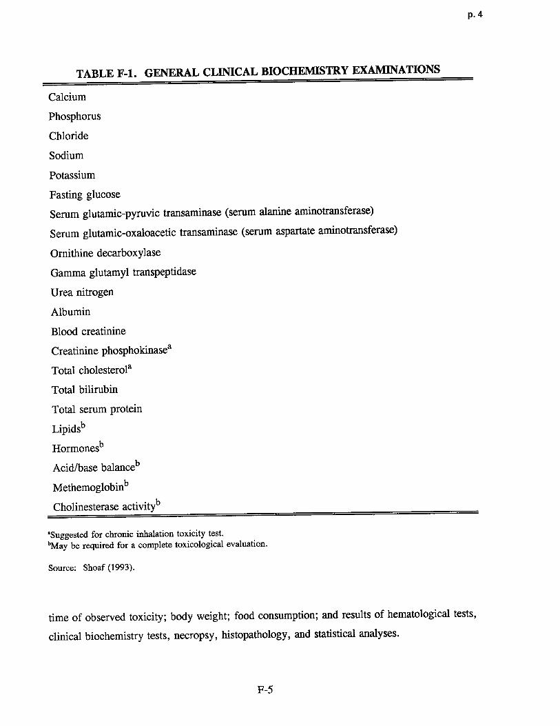
should dictate the repertoire of tests performed, Table F-1 provides a general list of
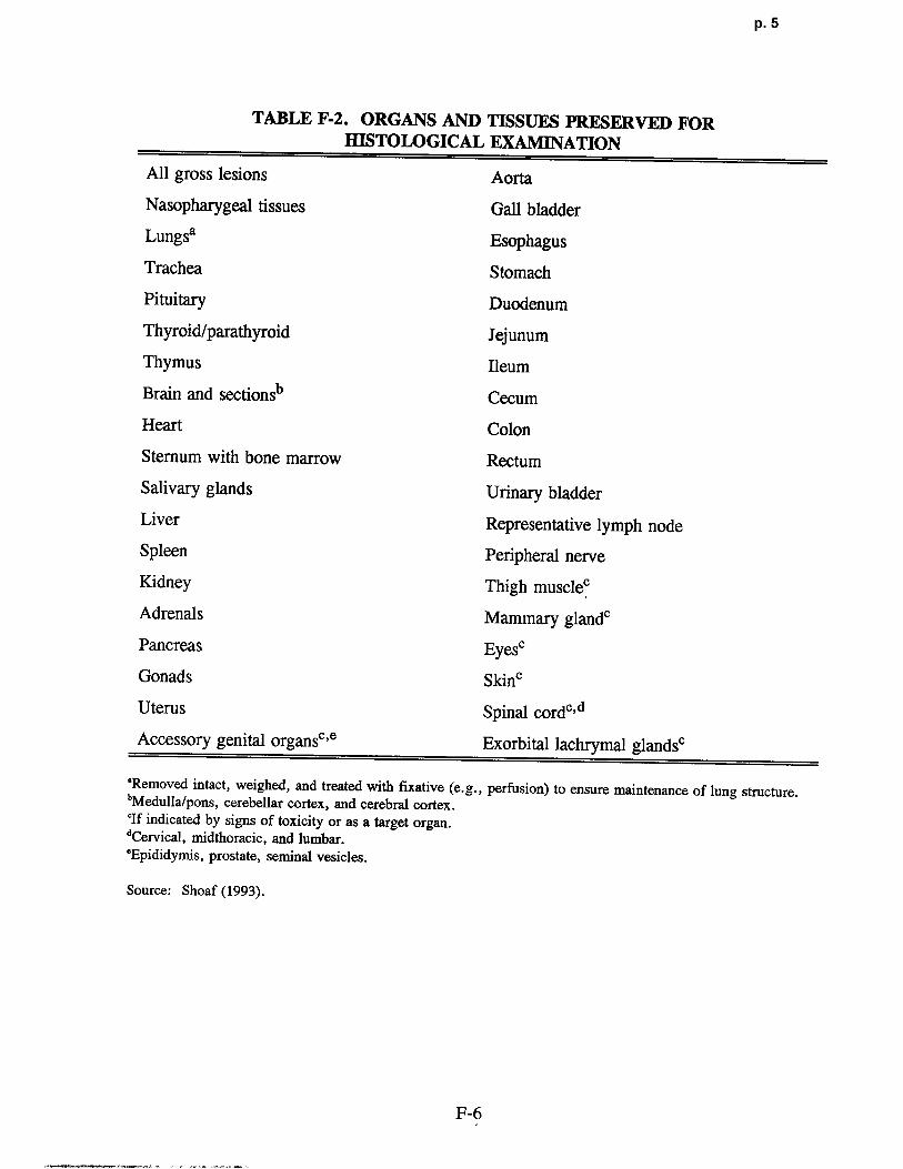
recommended clinical biochemistry examinations ; and Table F-2 provides a list of organs and
tissues recommended for histological examination . If specific mechanisms of action are
hypothesized, specific assays or functional tests for those would be added . It is also
important to establish that appropriate removal and tissue processing was performed .
Results should be reported in tabular form, showing the number of animals at test start,
number with lesions, the types of lesions, and the percentage of animals with each type.
Group animal data should be reported to show number of animals dying, number showing
signs of toxicity, and number exposed . Individual animal data should include time of death ;
F-4
p. 4
TABLE F-1 . GENERAL CLINICAL BIOCHEMISTRY EXAMINATIONS
Calcium
Phosphorus
Chloride
Sodium
Potassium
Fasting glucos e
Serum glutamic-pyruvic transaminase (serum alanine aminotransferase)
Serum glutamic-oxaloacetic transaminase (serum aspartate aminotransferase)
Ornithine decarboxylase
Gamma glutamyl transpeptidase
Urea nitrogen
Albumin
Blood creatinine
Creatinine phosphokinasea
Total cholesterola
Total bilirubin
Total serum protein
Lipidsb
Hormonesb
Acid/base balanceb
Methemoglobinb
Cholinesterase activityb
'Suggested for chronic inhalation toxicity test .
'May be required for a complete toxicological evaluation .
Source: Shoaf (1993) .
time of observed toxicity ; body weight ; food consumption ; and results of hematological tests,
clinical biochemistry tests, necropsy, histopathology, and statistical analyses .
F-5
p. 5
TABLE F-2 . ORGANS AND TISSUES PRESERVED FO RHISTOLOGICAL EXAMINATION
All gross lesions Aorta
Nasopharygeal tissues Gall bladder
Lungsa Esophagus
Trachea Stomach
Pituitary Duodenum
Thyroid/parathyroid Jejunum
Thymus Ileum
Brain and sectionsb Cecum
Heart Colon
Sternum with bone marrow Rectum
Salivary glands Urinary bladder
Liver Representative lymph node
Spleen Peripheral nerve
Kidney Thigh muscie°
Adrenals Mammary glandc
Pancreas Eyes'
Gonads Skin°
Uterus Spinal cord"
Accessory genital organs° ,e Exorbital lachrymal glandsc
'Removed intact, weighed, and treated with fixative (e .g., perfusion) to ensure maintenance of lung structure .bMedulla/pons, cerebellar cortex, and cerebral cortex .°If indicated by signs of toxicity or as a target organ .'Cervical, midthoracic, and lumbar .`Epididymis, prostate, seminal vesicles .
Source: Shoaf (1993) .
F-6
p. 6
APPENDIX G
THE PARTICLE DEPOSITIONDOSIMETRY MODEL
In this appendix, the revised empirical model used to estimate fractional regional
deposition efficiency for calculation of RDDR (Equation 4-5) to be used as a dosimetric
adjustment factor is described (Mdnache et al ., submitted) . This revised model represents
refinement of previously published models used to calculate the RDDR in the 1990 interim
RfC methods (Jarabek et al ., 1989, 1990 ; Miller et al., 1988) . For example, rather than
linear interpolation between the published (Raabe et al ., 1988) means for deposition measured
at discrete particle diameters, as previously done for the laboratory animal deposition
modeling, equations have now been fit to the raw data as described herein .
The equations to perform calculations for monodisperse particles are provided ; how the
calculated efficiencies may be transformed to fractional depositions is indicated ; how to use
the model to predict deposition fractions for polydisperse particles is explained ; and the
effects of the mass median aerodynamic diameter (MMAD) and the geometric standard
deviation (ag) on the regional deposited dose ratio (RDDRr) calculations are illustrated .
Because VE must be calculated from the default body weights (Table 4-5) using allometric
scaling (Equation 4-4) for use as input to the empirical model, the example of hand
calculation of monodisperse deposition includes a VE calculation .
Fractional deposition of particles in the airways of the respiratory tract may be
estimated using theoretical or empirical models or some combination of the two . Progress is
being made in answering the data needs of theoretical models (e .g ., exact airflow patterns,
complete measurements of the branching structure of the respiratory tract, pulmonary region
mechanics), however, many uncertainties remain. Empirical models are systems of equations
that are fit to experimentally determined deposition in vivo . These models do not require the
detailed information needed for theoretical models, however, they can not provide estimates
of dose to localized specific sites (e .g., respiratory versus olfactory nasal epithelium terminal
bronchioles, carinal ridges) . Measurement techniques are such that only general regions can
G-1

p. 7
be defined (Stahlhofen et al., 1980; Lippmann and Albert, 1969 ; Raabe et al, 1977) which
limits the regions that can be defined for a dosimetry model . Despite this level of generality,
regional information is available now for humans and a number of commonly used laboratory
animals . Empirical models of regional fractional deposition have been presented for humans
(Yu et al ., 1981 ; Miller et al ., 1988; Stahlhofen et al ., 1989). The empirical model
described in this appendix was fit for five species of commonly used laboratory rodents using
experimental data received from Dr . Otto Raabe (Raabe et al ., 1988) . At the same time ,
Dr. Morton Lippmann (Lippmann and Albert, 1969 ; Lippmann, 1970, 1977 ; Chan andLippmann, 1980; Miller et al., 1988) and Dr . Wilhelm Stahlhofen and colleagues (Stahlhofen
et al ., 1980, 1983, 1989 ; Heyder and Rudolf, 1977; Heyder et al ., 1986) provided the
individual experimental measurements from their published studies. Using these data, the
human model published in Miller et al . (1988) was extended by refitting the extrathoracic
(ET) (oral breathing) and tracheobronchial (TB) deposition efficiencies with the original raw
data as well as by fitting a pulmonary (PU) deposition efficiency equation (Menache et al .,submitted) .
G .1 EMPIRICAL MODEL FOR REGIONAL FRACTIONALDEPOSITION EFFICIENCIE S
The equations describing fractional deposition were fit using data on particle deposition
in CF1 mice, Syrian golden hamsters, Fischer 344 rats, Hartley guinea pigs, and New
Zealand rabbits . A description of the complete study including details of the exposure may
be found elsewhere (Raabe et al ., 1988) . Briefly, the animals were exposed to radiolabelled
ytterbium (169Yb) fused aluminosilicate spheres in a nose-only exposure apparatus . Twenty
unanesthetized rodents or eight rabbits were exposed simultaneously to particles of
aerodynamic diameters (dae) about 1, 3, 5, or 10 µm. Half the animals were sacrificed
immediately post exposure ; the remaining half were held 20 h post exposure . One-half of the
animals at each time point were male and the other half were female . The animals were
dissected into 15 tissue compartments, and radioactivity was counted in each compartment .
The compartments included the head, larynx, GI tract, trachea, and the five lung lobes . This
information was used directly in the calculation of the deposition fractions . Radioactivity was
G-2
p. 8
also measured in other tissues including heart , liver, kidneys, and carcass ; and additionally in
the urine and feces of a group of animals held 20 hours. In the an imals sacrificed
immediately post exposure, these data were used to ensure that there was no contamination of
other tissue while the data from the animals held 20 hours were used in the calcula tion of a
fraction used to parti tion thoracic deposition between the TB and PU regions. This partition
is discussed below briefly and described in detail elsewhere (Raabe et al ., 1977) . Finally,
radioactivity was measured in the pelt, paws, tail, and headskin as a control on the exposure .
Although there are some other studies of particle deposi tion in laboratory animals (see
review by Schlesinger, 1985), no other data have the level of detail or the expe rimental
design ( i .e., freely breathing, unanesthetized, nose-only exposure) required to provide
deposition equations representative of the animal exposures used in many inhalation
toxicology studies . However, many inhalation toxicology studies are not nose-only
exposures . While this is a necessary exposure condi tion to determine fractional particle
deposi tion, adjustments for particle inhalability and ingestion can be made to es timate
deposition fractions under whole-body exposure condi tions .
The advantages of using the data of Raabe et al . (1988) to develop the deposi tion
equations include :
• the detailed measurements were made in all tissues in the animal, providing mass
balance information and indicating that there was no contamination of nonrespirato ry
tract tissue with radioactivity immediately post exposure ,
• the use of five species of laborato ry animals under the same exposure conditions,
• the use of unanesthetized, freely breathing an imals, and
• the use of an exposure protocol that makes it vi rtually impossible for the animals to
ingest any particles as a result of preening .
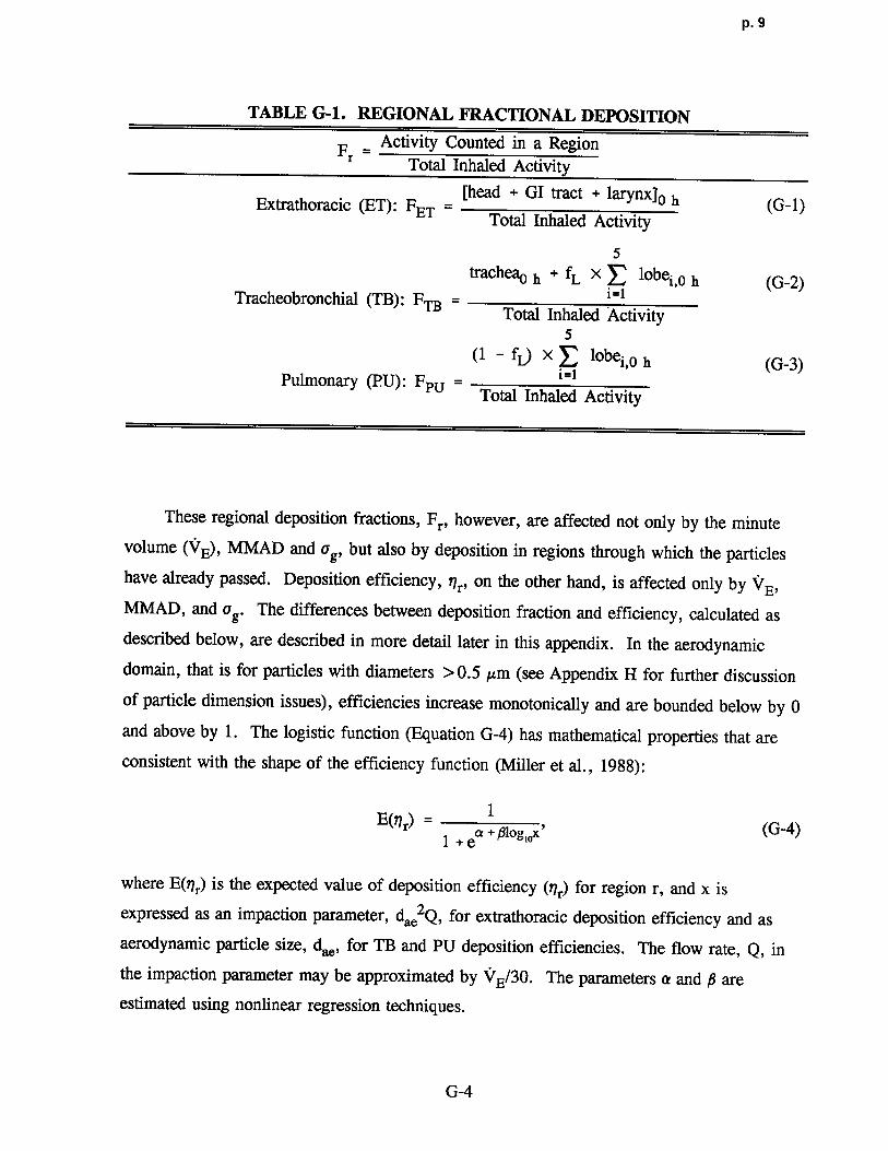
Regional fractional deposition, Fr, was calculated as activity counted in a region
normalized by total inhaled activity (Table G-1) . The proportionality factor, fL, in Equations
G-2 and G-3 is used to partition thoracic deposition between the TB and PU regions. It was
calculated using the 0 and 20-h data and is described in detail by Raabe and co-workers
(1977) .
G-3
p. 9
TABLE G-1 . REGIONAL FRACTIONAL DEPOSITION
F= Activity Counted in a Regionr Total Inhaled Activity
[head + GI tract + larynx]o hExtrathoracic (ET): FET = (G-1)Total Inhaled Activity
5trachea0 h + fL X lobei,o h (G-2)
Tracheobronchial (TB) : FTB = i=1Total Inhaled Activity
5(1 - fL) X lobei,o h (G-3)
Pulmonary (PU) : FpU = i=1Total Inhaled Activity
These regional deposition fractions, Fr, however, are affected not only by the minute
volume (VF), MMAD and ag, but also by deposition in regions through which the particles
have already passed . Deposition efficiency, rlr, on the other hand, is affected only by VE,
MMAD, and vg . The differences between deposition fraction and efficiency, calculated as
described below, are described in more detail later in this appendix . In the aerodynamic
domain, that is for particles with diameters > 0 .5 µm (see Appendix H for further discussion
of particle dimension issues), efficiencies increase monotonically and are bounded below by 0
and above by 1 . The logistic function (Equation G-4) has mathematical properties that are
consistent with the shape of the efficiency function (Miller et al ., 1988):
E(t7r) = 11 +e a + fi1og , oR
,(G-4)
where E(r7 r) is the expected value of deposition efficiency (r7r) for region r, and x is
expressed as an impaction parameter, dae2Q, for extrathoracic deposition efficiency and as
aerodynamic particle size, dae, for TB and PU deposition efficiencies . The flow rate, Q, in
the impaction parameter may be approximated by VE/30 . The parameters a and fi are
estimated using nonlinear regression techniques .
G-4
P. 10
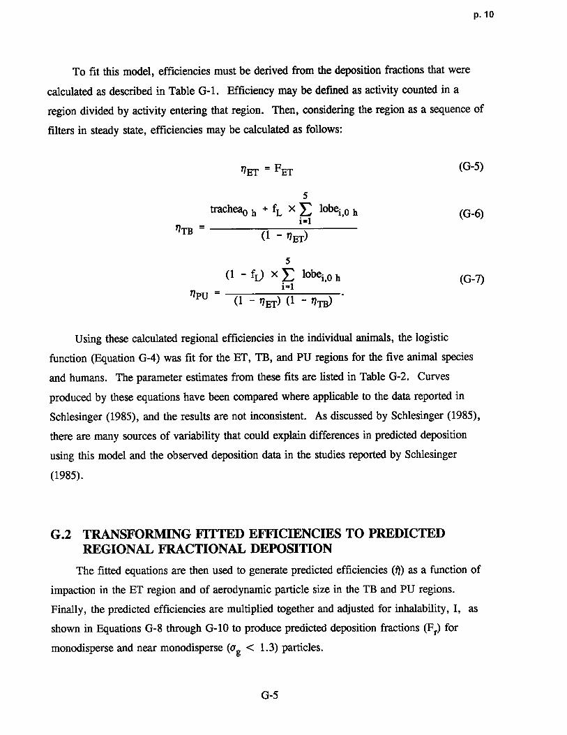
To fit this model, efficiencies must be derived from the deposition fractions that were
calculated as described in Table G-1 . Efficiency may be defined as activity counted in a
region divided by activity entering that region . Then, considering the region as a sequence of
filters in steady state, efficiencies may be calculated as fo llows :
nET = FET(G-5)
5
tracheao h + fL x lobei,0 h (G-6)i=1
'7TB _ - (1 -t1ET)
5
(1 - U x lobei,0 h (G-7)i=1
1]PU = (1 - nET) (1 - nTB
)
Using these calculated regional efficiencies in the individual animals, the logistic
function (Equation G-4) was fit for the ET, TB, and PU regions for the five animal species
and humans. The parameter estimates from these fits are listed in Table G-2 . Curves
produced by these equations have been compared where app licable to the data reported in
Schlesinger (1985), and the results are not inconsistent . As discussed by Schlesinger (1985),
there are many sources of variability that could explain differences in predicted deposition
using this model and the observed deposition data in the studies reported by Schlesinger
(1985) .
G.2 TRANSFORMING FITTED EFFICIENCIES TO PREDICTEDREGIONAL FRACTIONAL DEPOSITIO N
The fitted equations are then used to generate predicted efficiencies (~) as a function of
impaction in the ET region and of aerodynamic particle size in the TB and PU regions .
Finally, the predicted efficiencies are multiplied toge ther and adjusted for inhalability, I, as
shown in Equations G-8 through G-10 to produce predicted deposition fractions (Fr) for
monodisperse and near monodisperse (Qg < 1 .3) particles .
G-5

P . 11
TABLE G-2. DEPOSITION EFFICIENCY EQUATIONESTIMATED PARAMETERS
ET (Nasal) TB PU
Species a p a P aHuman 7.129a -1.957a 3.298 -4.588 0.523 -1 .389Rat 6.559 -5.524 1.873 -2.085 2.240 -9 .464Mouse 0.666 -2.171 1.632 -2.928 1 .122 -3.196Hamster 1.969 -3.503 1 .870 -2.864 1.147 -7.223Guinea Pig 2.253 -1.282 2.522 -0.865 0.754 0.556Rabbit 4.305 -1.628 2.819 -2.281 2.575 -1 .988
'Source : Miller et al ., 1988 .
FET = I X ~ET (G-8)
AFTB = I X (1 - ;~E1) x ;~TB (G-9)
FpU = I X (1 - i~ET)X (1
- i7TB) XPU (G-10)
Inhalability, I, is an adjustment for the particles in an ambient exposure concentration
that are not inhaled at all . For humans, an equation has been fit using the logistic function
(Menache et al ., 1995) . Using the experimental data of Breysse and Swift (1990) :
I = 1 - 11 + e10.32-7.17 logiod (G-11).
The logistic function was also fit to the data of Raabe et al . (1988) for laboratory animals
(Mdnache et al., 1995) :
I = 1 -1
1 + e2.57-2.81 logtod (G-12).
G-6

p. 12
For example, calculation of FPU for a female Syrian golden hamster exposed to a nearly
monodisperse particle (ag < 1 .3) with an MMAD of 1 .8 in a subchronic study would
proceed as follows .
1 . Calculate the default VE. (If the study for which the RDDRPU is being calculatedhas information on experimentally measured VE, that information may besubstituted for the default value ; however, this could necessitate changes to surfaceareas and body weight (if extrarespiratory tract effects are being examined) .
If there is inadequate information to change all of these values, then the default
values should be used . )
a. The default body weight for a female Syrian hamster in a subchronic study fromTable 4-4 is 0 .095 kg .
b . Calculation of VE expressed in natural logarithms using hamster coefficients
from Table 4-5 :
log (VE) _ -1 .054 + 0.902 X log (0.095)_ -3.177
c. Convert from natural logs to arithmetic units
exp (-3.177) = 0.041 7
d. Convert from L to mL by multiplying by 1,000
VE = 41 .7
2 . Calculate the impaction parameter as MMAD2 X VE/30 for the ET region
= (1 .8)2 X (41 .7/30)= 4.504and take the loglo= 0.654
3 . Calculate nET using the parameters from Table G-2
= 1/(1 + exp(l .969 - 3 .503 x 0.654))= 0.580
G-7
p. 13
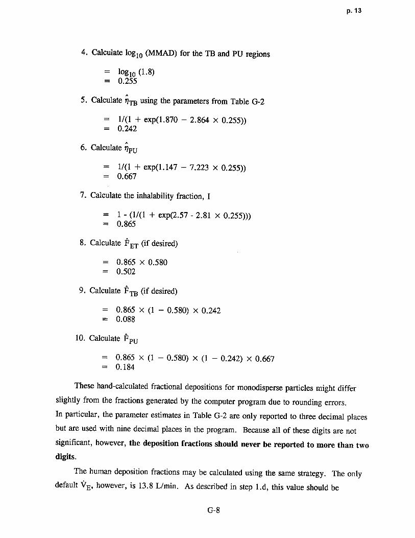
4. Calculate loglo (MMAD) for the TB and PU region s
= loglo (1 .8)= 0.255
5 . Calculate '?TB using the parameters from Table G-2
= 1/(1 + exp(1 .870 - 2 .864 x 0.255))= 0.242
6. Calculate ripU
= 1/(1 + exp(1 .147 - 7.223 x 0.255))= 0 .667
7 . Calculate the inhalability fraction, I
= 1-(1/(1 + exp(2.57 - 2.81 x 0.255)))= 0. 865
8 . Calculate FET (if desired)
= 0.865 x 0 .580= 0.502
9. Calculate FFTB (if desired)
= 0.865 x (1 - 0.580) x 0 .242= 0 .088
10. Calculate Fp U
= 0.865 x(1 - 0.580) x(1 - 0.242) x 0 .667= 0.184
These hand-calculated fractional depositions for monodisperse particles might differ
slightly from the fractions generated by the computer program due to rounding errors .
In particular, the parameter estimates in Table G-2 are only reported to three decimal places
but are used with nine decimal places in the program. Because all of these digits are not
significant, however, the deposition fractions should never be reported to more than two
digits .
The human deposition fractions may be calculated using the same strategy. The only
default VE, however, is 13 .8 L/min. As described in step 1 .d, this value should be
G-8
p. 14
converted to mL by multiplying by 1,000 . The information provided in Table G-2 allows fo r
estimation of deposition in humans for nasal breathing only . When exercising (VE greater
than 35 L/min), a portion of the inhaled air will enter through the mouth . The ET deposition
efficiencies for oral breathing are different from those for nasal breathing and are not
recorded in Table G-2 . They are, however, included in the computer program as well as
proportionality factors defining flow splits between the nose and mouth at higher VE. The
additional complexities engendered in the calculation of the ET deposition fraction when both
oral and nasal breathing are involved are such that those calculations should not be performed
by hand.
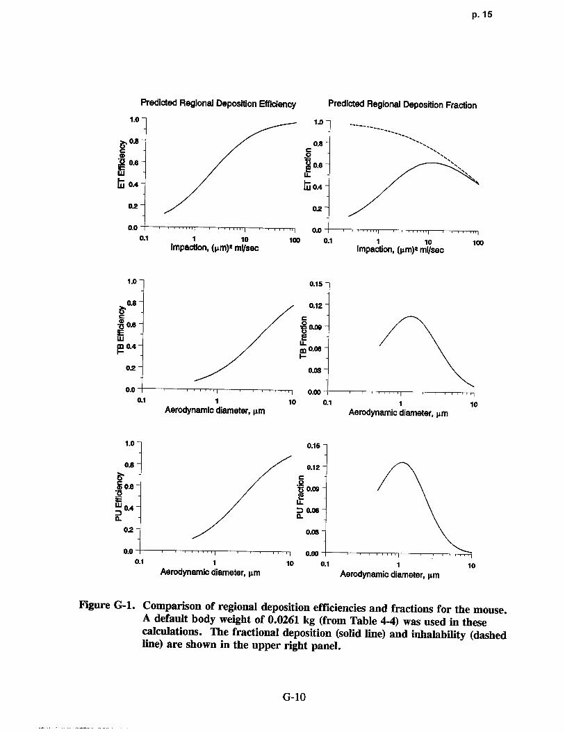
Figure G-1 illustrates the relationship between the predicted efficiencies and predicted
depositions using this model for the mice . A qualitatively similar set of curves could be
produced for any of the other four species . The calculations were made according to the
ten steps listed above. The particles were assumed to be monodisperse and the default body
weight (BW) for the mice, taken from Table 4-4, was 0 .0261 kg . This is the default BW of
male BAF1 mice for chronic exposure study durations . Regional deposition efficiencies and
fractions were calculated for particles with dae ranging from 0 .5 to 10 µm. These calculated
points were connected to produce the smooth curves shown in Figure G-1 . The three panels
on the left of Figure G-1 are plots of the predicted regional deposition efficiencies ; the three
panels on the right show the predicted regional deposition fractions derived from the
estimated efficiencies and adjusted for inhalability . The vertical axis for the predicted
deposition efficiency panels range from 0 to 1 . Although the deposition fraction is also
bounded by 0 and 1, the vertical axes in the figure are less than 1 in the TB and PU regions .
The top two panels of Figure G-1 are the predicted deposition efficiency and fraction,
respectively, for the ET region . These two curves are plotted as a function of the impaction
parameter described for Equation G-4 . The middle two and lower two panels show the
predicted deposition efficiencies and fractions for the TB and PU regions, respectively .
These four curves are plotted as a function of dae. When a particle is from a monodisperse
size distribution, the dae and the MMAD are the same . If, however, the particle is from a
polydisperse size distribution, the particle can not be described by a single dae ; the average
value of the distribution, the MMAD, must be used. (See Appendix H for further discussion
of particle sizing, units, and averaging methods) . In the aerodynamic particle size range, the
G-9
p. 15
Predicted Regional Deposition Efficiency Predicted Regional Deposition Fraction
1 .0 1 .0-
.8 0.8-0
0.6 06W LL~j OA LU- OA
02 02-
0.00.0
0.1 1 10 100 0.1 1 10 100Impaction, (pm) g ml/sec Impaction, (µm)Y ml/sec
1 .0 0.15-
0.8- 0.12-
00-6- 0.09-
ME LELM 0.4 0.08
0.2- 0.03-
0-00.0 0-00-0.1 1 10 0.1 1 10
Aerodynamic diameter, µm Aerodynamic diameter, pm
1.0 0.15
02 0.1 2
a0.6 °'J3 0.09
? OA a 0.06IL
0.2- 0.03-
0.0- 10.0 o.ao0.1 1 10 0.1 1 10
Aerodynamic diameter, pm Aerodynamic diameter, pm
Figure G-1 . Comparison of regional deposition efficiencies and fractions for the mouse .A default body weight of 0 .0261 kg (from Table 4-4) was used in thesecalculations . The fractional deposition (solid line) and inhalability (dashedline) are shown in the upper right panel .
G-10

p. 16
deposition efficiency curves all increase monotonically as a function of the independen t
variable (i .e., either the impaction parameter or d.) and have both lower and upper
asymptotes . The curves describing the deposition fractions, however, have different shapes
that are dependent on the respiratory tract region . Deposition fractions in all three regions
are nonmonotonic-initially increasing as a function of particle size but decreasing as particle
sizes become larger . This is because particles that have been deposited in proximal regions
are no longer available for deposition in distal regions . As an extreme example, if all
particles are deposited in the ET region, no particles are available for deposition in either the
TB or PU regions . In the ET region, the nonmonotonic shape for fractional deposition is due
to the fact that not all particles in an ambient concentration are inhalable .
G.3 POLYDISPERSE PARTICLES
As discussed in Appendix H, particles in an experimental or ambient exposure are
rarely all a single size but rather have some distribution in size around an average value .
As this distribution becomes greater, the particle is said to be polydisperse . Panel A of
Figure G-2 illustrates the range of particle sizes from a distribution that is approximately
monodisperse (Qg = 1 .1) and particles that come from a lognormal highly polydisperse
distribution (Qg = 3.0), although both distributions have the same MMAD of 4 .0 µm. Also
drawn in Panel A of Figure G-2 is a vertical line through the MMAD that represents the
extreme case of ag = 1 .0, that is, an exact monodisperse particle distribution in which all
particles are a single size, which is also the MMAD .
The empirical model described in this appendix was developed from exposures using
essentially monodisperse particles (which are treated as though they are exactly
monodisperse) . It is therefore possible to multiply the particle size distribution function
(which is customarily considered to be the lognormal distribution) by the predicted
depositions (calculated as described in Equations G-8 through G-10) and integrate over the
entire particle size range (0 to -*) . Mathematically, this calculation is performed as described
by Equation G-3, and is illustrated for the mouse and human ET regions in panels B and C
respectively, of Figure G-2 .
G-11

p. 17
Kdee)5- Lognormal Distribution
aq-1.0 MMAD4.Oµm
4
9
i2 ap
aQ-3.0
00 10 20 80 40 so so
Aerodynamic Diameter (dad, µ m
1 .0 Extrathorack Deposition (B) 1 .0 Ex tratfroradc Deposition (C~Mouse C Human
o °OB
LL LL
~ ag 1.0 ~ ----
--------0A a93.0 0,{
ru rii ap 3.0
02 0,2
ao1 .00.0 OJO
0.1 1 10 0.1 10MMAD,µm MMAD, pm
Figure G-2. Range of particles for lognormal distributions with same ACV" butdiffering geometric standard deviations (A). Effect of polydisperseparticles on predicted extrathoracic deposition fractions in mice (B) andhumans (C) .
_ CO 1 (logd logMMAD)2 (G-13)[Fr] [Fr]m X X exp -1/2 ae ddae
0 f dae(logQg ) 27[ logQg ae
where log refers to the natural logarithim, [Fr]p is the predicted polydisperse fractional
deposition for a given MMAD, and [Fr]m is the predicted monodisperse fractional deposition
for particles of size dae . The limits of integration are defined from 0 to w but actually include
only four standard deviations (99 .95% of the complete distribution) . For each particle size inA
the integration, [Fr]m is calculated as described in the ten steps listed in this appendix, then
G-12
p. 18
multiplied by the probability of observing a particle of that size in a particle size distribution
with that MMAD and Qg .
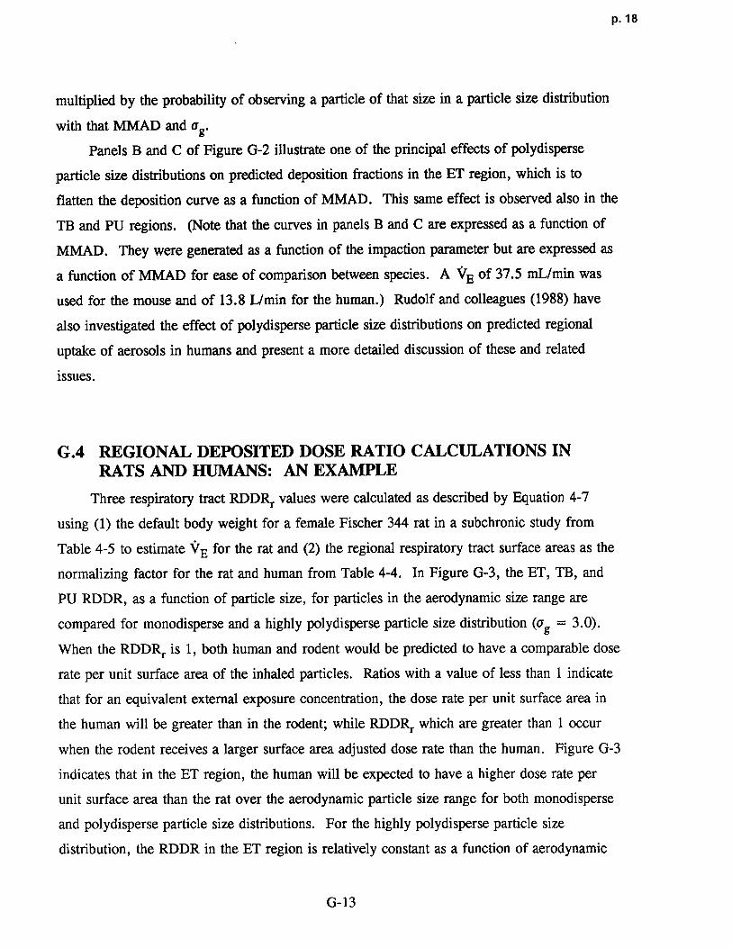
Panels B and C of Figure G-2 illustrate one of the principal effects of polydisperse
particle size distributions on predicted deposition fractions in the ET region, which is to
flatten the deposition curve as a function of MMAD . This same effect is observed also in the
TB and PU regions . (Note that the curves in panels B and C are expressed as a function of
MMAD. They were generated as a function of the impaction parameter but are expressed as
a function of MMAD for ease of comparison between species . A VE of 37.5 mL/min was
used for the mouse and of 13.8 L/min for the human.) Rudolf and colleagues (1988) have
also investigated the effect of polydisperse particle size distributions on predicted regional
uptake of aerosols in humans and present a more detailed discussion of these and related
issues .
G.4 REGIONAL DEPOSITED DOSE RATIO CALCULATIONS INRATS AND HUMANS: AN EXAMPLE
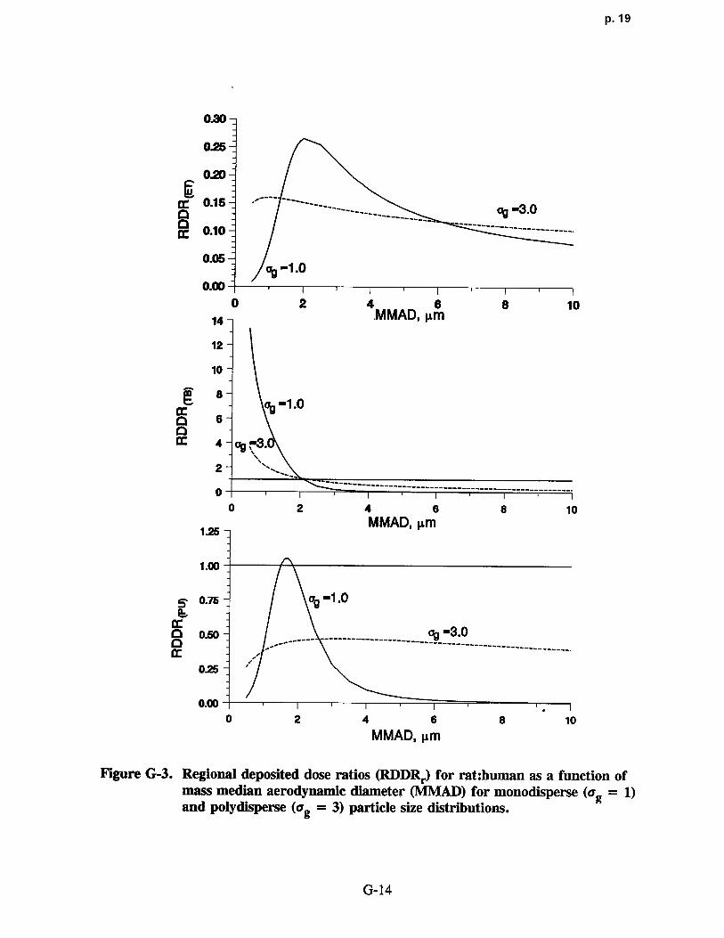
Three respiratory tract RDDRr values were calculated as described by Equation 4-7
using (1) the default body weight for a female Fischer 344 rat in a subchronic study from
Table 4-5 to estimate VE for the rat and (2) the regional respiratory tract surface areas as the
normalizing factor for the rat and human from Table 4-4 . In Figure G-3, the ET, TB, and
PU RDDR, as a function of particle size, for particles in the aerodynamic size range are
compared for monodisperse and a highly polydisperse particle size distribution (vg = 3 .0) .
When the RDDRr is 1, both human and rodent would be predicted to have a comparable dose
rate per unit surface area of the inhaled particles . Ratios with a value of less than 1 indicate
that for an equivalent external exposure concentration, the dose rate per unit surface area in
the human will be greater than in the rodent ; while RDDRr which are greater than 1 occur
when the rodent receives a larger surface area adjusted dose rate than the human . Figure G-3
indicates that in the ET region, the human will be expected to have a higher dose rate per
unit surface area than the rat over the aerodynamic particle size range for both monodisperse
and polydisperse particle size distributions . For the highly polydisperse particle size
distribution, the RDDR in the ET region is relatively constant as a function of aerodynami c
G-13
P. 19
0.30-
0.25-
0.20-
0.15--3.0o ' - --- - ----------- ---------------------------
0.10-
0.05-01 a9 -1 0
0.0
0 2 4.MMAD, µm S 1014
12-
10-
8--1 .0
p 6
2 ~.
-----------------------------------------------------
0 2 4 6 8 10
1.25MMAD, µm
1 .00
0.7s v9 -1 .0
0.50 ---- ------------------------~ 3--------------------------
025
0.000 2 4 6 8 10
MMAD, µ m
Figure G-3 . Regional deposited dose ratios (RDDRd for rat :human as a function ofmass median aerodynamic diameter (NIlVIAD) for monodisperse (ag = 1)and polydisperse (ag = 3) particle size distributions .
G-14

p. 20
particle size . This may be interpreted to mean that for a highly polydisperse size distribution,
the dose rate per unit surface area to the ET region of the human will be approximately 10 to
15 times that to the ET region of the rat regardless of the particle MMAD . In the TB region,
the RDDR declines over the aerodynamic particle size range for both mono- and polydisperse
particle size distributions . For particles smaller than about 2 µm MMAD, the rat is predicted
to have a higher dose rate than the human ; for larger particles, the relationship is reversed.
In the PU region, a relationship that is qualitatively similar in shape to the RDDRET is
observed; however, the range of the RDDRpU is much larger and there is a suggestion that
the dose rate in the rat is greater than that in the human for particles of about 2 µm MMAD
since the RDDRpU > 1 .0 .
This example illustrates the complexities in the relationships between dose rate per unit
surface area in the three respiratory tract regions for rodents and humans . The regional
differences as well as the differences due to MMAD and a9 indicate the importance of
replacing administered dose with dosimetric information whenever possible in making risk
evaluations .
G-15
p. 21
APPENDIX H
PARTICLE SIZING CONVENTIONS
Solid or liquid particles suspended in a gas are called an aerosol . In toxicological
experiments and epidemiological studies, aerosol particles from a given exposure are
commonly described by some measure of the average size of the particle and some measure
of variability in that average size . Although the average size is usually expressed as a
diameter, there are numerous methods for calculating diameter . In this appendix, some of
the more common sizing conventions for spherical (or nearly spherical) particles are briefly
discussed . Conversions from reported units to the units required to use the particle dosimetry
model described in this document are provided . More detailed discussions of particle
properties and behavior may be found elsewhere (Raabe, 1971, 1976 ; Hinds, 1982).
H.1 GENERAL DEFINITIONS
Particles in an exposure are rarely all a single size but rather have some distribution in
size around an average value . It is generally accepted (Raabe, 1971) that the lognormal
distribution provides a reasonable approximation for most observed spherical particle
distributions . For this reason, particle exposures are frequently characterized by median
diameter and the geometric standard deviation (Qg). Statistically speaking, data from a
lognormal distribution may be completely described by the median and geometric standard
deviation. As ag approaches 1 .0, the distribution of the particles approaches a single size and
the particles are said to be monodisperse . As a matter of practicality, a distribution is
considered to be near monodisperse when Qg is less than 1 .3 . As Qg approaches infinity, the
distribution contains particles of many sizes and is said to be polydisperse . By definition ,
vg cannot be less than 1 .0 .
In toxicological experiments, researchers might use (or try to use) monodisperse
spherical particles because deposition is a function of particle size . Real world exposures,
however, are rarely to monodisperse particles . Accordingly, laboratory animal experiments
H-1
p. 22
designed to mimic some real exposure will use polydisperse pa rt icle distributions. Studies of
diesel exhaust and of Mt. St. Helens volcanic ash, for example, used highly polydisperse
particles. In addition to being polydisperse, such pa rticles also have irregular shapes . .
Although some irregular particles may be described by their aerodynamic diameter and so be
considered to behave like spherical particles, other particles have such extreme differences in
shape that they must be described by other parameters . Fibers are one extreme example of
nonspherical particle shapes. Deposition fractions for these particles may not be calculated
with the particle dosimetry model used in the methodology .
Particle diameters are most frequently reported as geomet ric diameter (dg) or
aerodynamic diameter (dae) . Aerodynamic diameter is defined as - the diameter of a unit
density sphere having the same settling velocity as the geomet ric diameter of the particle inquestion . Geometric diameters may be converted to aerodynamic diameters according to the
following equation :
dae = dg pC(dg)/C(dae) = dgFp , (H-1)
where p is the particle density in g/cm3 and C(d) is the Cunningham slip correction factor .
The particle dosimetry model requires that the particle size be expressed in aerodynamic
diameter so studies reporting particle sizes in these units will most likely not require any
further conversion . There are, however, two commonly used definitions for dae ; the
methodology uses the definition of the Task Group on Lung Dynamics (1966) . Because of
the complexities in calculating dae by the Task Group equation, other investigators have
developed an alternate specification for aerodynamic diameter (Mercer et al ., 1968 ; Raabe,
1976) . This dae is called an aerodynamic resistance diameter, dar, and may be converted to
dae according to the following equation :
dae = (dar2 +0.0067)0.5 - 0 .082 . (H-2)
H-2

p. 23
Summary information from an exposure will most often be presented as count (CMD) ,
mass (MMD), surface (SMD) or activity (AMD), median (geometric) diameter . The
summary information might be reported in terms of median aerodynamic diameters instead
(CMAD, MMAD, SMAD, AMAD) .
Because the particle distributions are assumed to be lognormal, estimation of count,
surface area, or mass distributions for any given sample of particles may be made once one
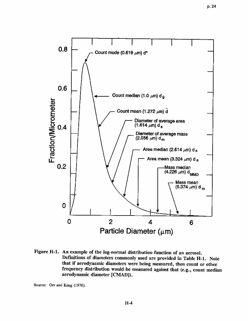
of those distributions has been measured . Figure H-1 shows a typical log-normal distribution
and the various indicated diameters encountered in inhalation toxicology literature .
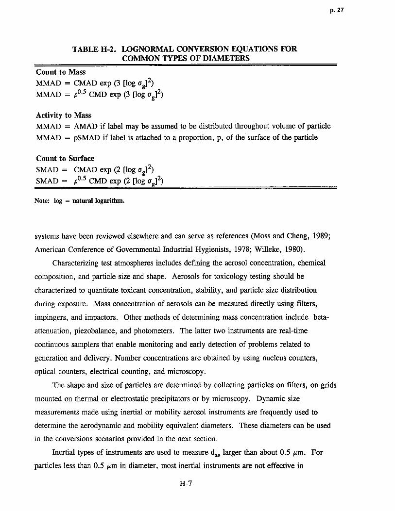
Table H-1 provides the definitions of these diameters . A series of conversion equations
originally derived by Hatch and Choate (1929) may be used to convert the reported units to
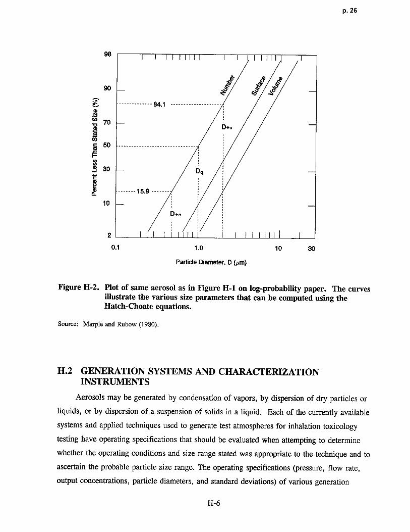
MMAD, the units required by the particle dosimetry model . Figure H-2 shows the same
aerosol as in Figure H-i plotted on log-probability paper and illustrates the various size
parameters that can be computed using the Hatch-Choate equations . The relevant conversion
equations are summarized in Table H-2 . It is a characteristic of any weighted distribution of
a lognormal distribution (such as the conversions described in Table H-2) that the geometric
standard deviation will be unchanged .
Conversion of activity median diameter (AMD) to MMAD depends on how the
radiolabeling of the particle was done . If the label was generated in a liquid, then the label is
distributed throughout the volume of the particle and the AMAD may be considered to be
equivalent to the MMAD . If, however, the radioactivity was attached to the surface of the
particle, then the activity median diameter may be considered to be proportional to the
surface area median diameter . More information on the labelling procedure is required to
provide an estimate of the proportionality factor . Further discussion of issues related to
activity diameters may be found elsewhere (Hofmann and Koblinger, 1989) .
The concept of activity diameter is also useful when considering the physical
characteristics of particles that are responsible for the health effect or toxicity of concern .
The activity diameter of a particle may be the most appropriate expression of size for this
purpose . This expression takes into account the "activity" of the physical property of the
particle. For example, if the toxicant is distributed only on the surface, then the activity
median diameter is equal to the surface median diameter ; and conversions to MMAD would
H-3
p. 24
0 . 8 Count mode (0 .619 ,um) d*
0 .6Count median ( 1 .0 Fcm) d g
i(DQD Count mean (1 .272 µm) dE0 Diameter of average area~ 0.4 (1 .614 gm) d a
Diameter of average mass(2.056 pm) d mC:
0
~ Area median (2.614 gm) d a
~ Area mean (3.324 ~.cm) d a
0.2 Mass median(4.226 pm) dMM D
Mass mean(5.374 pm) d m
0
0 2 4 6Particle Diameter (µm)
Figure H-1. An example of the log-normal distribution function of an aerosol .Definitions of diameters commonly used are provided in Table H-1 . Notethat if aerodynamic diameters were being measured, then count or otherfrequency distribution would be measured against that (e.g., count medianaerodynamic diameter [CMAD]) .
Source: Orr and Keng (1976) .
H-4

p. 25
TABLE H-1. PARTICLE DIAMETER DEFINITIONS
Count mode diameter The most frequently characterized particle diameter . In Figure H-1, thefrequency is normalized to frequency (or number) per micron . This type ofgraph is also used in analyzing cascade impactor data .
Count median diameter This diameter is used to describe any log-normal distribution . It is thediameter of a particle that is both larger and smaller than half the particles
sampled .
Count mean diameter The average particle diameter . It is calculated by first multiplying eachdiameter measured by the number of particles having that diameter .Summing all of these products over the entire range of diameters measuredand dividing by the total number of particles sampled gives the count meandiameter.
Diameter of "average mass" Another average particle diameter related to the total mass of particlessampled . The mass of the particle of "average mass" multiplied by thetotal number of particles sampled, equals the total mass of particlessampled . The total mass of particles sampled is calculated by firstmultiplying the single-particle mass calculated for each diameter measuredby the number of particles having that diameter and summing all of theseproducts over the entire range of diameters measured . The average mass ofeach individual particle sampled is obtained by dividing this number by thetotal number of particles. The diameter is calculated by assuming a sphereand applying the density of the material to convert from mass to volumeand then to diameter .
Mass median diameter Diameter of the particle having a mass that is both larger and smaller thanthe mass of half the particles sampled .
Mass mean diameter Average particle diameter, calculated by first multiplying each diametermeasured by the cumulative mass of all particles having that diameter .Summing all of these products over the entire range of diameters measuredand dividing by the total mass of the particles sampled gives the mass mean
diameter .
Source: Moss and Cheng (1989) .
be the same as described above for radiolabeled activity . If the toxicant is soluble, the
surface area of the particle will influence the rate of dissolution because solubilization occurs
at the surface . Such a situation needs to be understood more thoroughly, especially for
complex particles .
H-5
p. 26
98
ro`g ~m
90 ~
-------------- 84.1 -------------------
70D+a
50 ------------------------------IEco
30 Dq
------- 1 5 .9 -------a
10
D+o
2
0.1 1.0 10 30
Pa rticle Diameter, D ( ,um)
Figure H-2. Plot of same aerosol as in Figure H-1 on log-probabi lity paper . The curvesillustrate the various size parameters that can be computed using theHatch-Choate equations .
Source: Marple and Rubow (1980) .
H.2 GENERATION SYSTEMS AND CHARACTERIZATIONINSTRUMENTS
Aerosols may be generated by condensation of vapors, by dispersion of dry particles or
liquids, or by dispersion of a suspension of solids in a liquid . Each of the currently available
systems and applied techniques used to generate test atmospheres for inhalation toxicology
testing have operating specifications that should be evaluated when attempting to determine
whether the operating conditions and size range stated was appropriate to the technique and to
ascertain the probable particle size range . The operating specifications (pressure, flow rate,
output concentrations, particle diameters, and standard deviations) of various generatio n
H-6
p. 27
TABLE H-2 . LOGNORMAL CONVERSION EQUATIONS FORCOMMON TYPES OF DIAMETERS
Count to Mass
MMAD = CMAD exp (3 [log Qg]2)
MMAD = p0 . 5 CMD exp (3 [log Qg]2)
Activity to Mass
MMAD = AMAD if label may be assumed to be distributed throughout volume of particle
MMAD = pSMAD if label is attached to a proportion, p, of the surface of the particle
Count to Surface
SMAD = CMAD exp (2 [log Qg]2)
SMAD = p0 .5 CMD exp (2 [log uj2)
Note : log = natural logarithm .
systems have been reviewed elsewhere and can serve as references (Moss and Cheng, 1989 ;
American Conference of Governmental Industrial Hygienists, 1978 ; Willeke, 1980).
Characterizing test atmospheres includes defining the aerosol concentration, chemica l
composition, and particle size and shape . Aerosols for toxicology testing should be
characterized to quantitate toxicant concentration, stability, and particle size distribution
during exposure . Mass concentration of aerosols can be measured directly using filters,
impingers, and impactors . Other methods of determining mass concentration include beta-
attenuation, piezobalance, and photometers . The latter two instruments are real-time
continuous samplers that enable monitoring and early detection of problems related to
generation and delivery . Number concentrations are obtained by using nucleus counters,
optical counters, electrical counting, and microscopy .
The shape and size of particles are determined by collecting particles on filters, on grids
mounted on thermal or electrostatic precipitators or by microscopy . Dynamic size
measurements made using inertial or mobility aerosol instruments are frequently used to
determine the aerodynamic and mobility equivalent diameters . These diameters can be used
in the conversions scenarios provided in the next section .
Inertial types of instruments are used to measure dae larger than about 0 .5 µm. For
particles less than 0 .5 µm in diameter, most inertial instruments are not effective i n
H-7

p. 28
separating and measuring particle size. In these cases, the mobility type of aeroso l
instrument is used . The mobility equivalent diameter determines the collection efficiency in
many processes that are controlled by the diffusion deposition mechanism . Two types of
mobility instruments are the electrical aerosol analyzer (EAA) and the diffusion batteries .
No single instrument can measure aerosol size distributions of particles with diameters from
0.005 to 10 µm. Sometimes different exposure levels are generated or characterized with
different instruments . Careful analysis of data is required, because the inertial instruments
(e.g., cascade impactor) give mass distribution, and the EAA and screen diffusion battery
give number distribution . Figure H-3 shows the measurement ranges of aerosol monitoring
instruments : Knowledge of the measurement range of the instruments used to characterize
the test atmosphere can be useful in determining the probable particle size range used in a
given study .
Cascade Impactor
Low Pressure Cascade Impactor
EAA
Diffusion Battery or PFDB
Partide Diameter-00
0.00 1 0.01 0. 1 1 10 100
Impaction and Sedimentation
Diffusion
FIgure H-3 . Measurement ranges of aerosol monitoring instruments.
Source: Moss and Cheng (1989) .
H-8
p. 29
H.3 CONVERSION SCENARIOS
Particle information reported in a study will most likely fall into one of the seven
categories defined below. The remainder of this appendix describes these seven possibilities
and outlines appropriate strategies to convert reported particle information to MMAD,
required to run the particle dosimetry model .
1. MMAD and vg.
In this case the information in the study has been reported in the units required for
analysis, and no conversions or changes are required to run the model .
2. A median diameter and ag .
Conversions from the most commonly used medians to MMAD are provided in
Table H-2 . No conversions are required for Qg .
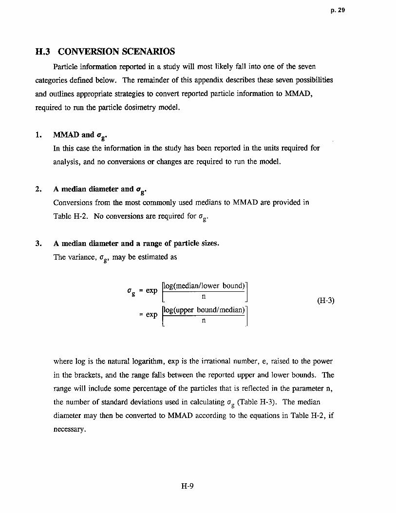
3. A median diameter and a range of part icle sizes .
The variance, vg, may be estimated a s
log(median/lower bound)Qg = exp
n (H-3)log(upper bound/median )
= expn
where log is the natural logarithm, exp is the irrational number, e, raised to the power
in the brackets, and the range falls between the reported upper and lower bounds . The
range will include some percentage of the particles that is reflected in the parameter n,
the number of standard deviations used in calculating Qg (Table H-3) . The median
diameter may then be converted to MMAD according to the equations in Table H-2, if
necessary .
H-9

p. 30
TABLE H-3. PERCENTAGE OF PARTICLES IN THE REPORTED RANGE
ASSOCIATED WITH THE NUMBER OF STANDARD DEVIATIONS (n)USED TO CALCULATE THE GEOMETRIC STANDARD DEVIATION
Percentage of Particlesin the Reported Range n
0.68 1
0.95 2
0.997 3
> 0.999 4
4. A median diameter only .
An estimate of vg must be derived from outside sources . In order of preference, the
following sources are recommended .
a: Other studies by the same group using the same compound for which the medianand Qg are reported .
b: A comparison of the variances reported by other studies for the same compoundcould be used to determine reasonable bounds on ag . Using the largest andsmallest vg determined by this method, the dosimetry model can be run todetermine the sensitivity of the dose ratio to vg for this particular particle sizeand rodent to human comparison .
c: The particle size range can be estimated from Figure H-4 and Qg calculatedaccording to Equation H-3 and Table H-3 (letting n = 4) . If necessary, themedian can then be converted to MMAD according to Table H-2 .
5. A range of particle sizes is the only information provided .
A median, in the same units as the reported particle size range, must be estimated from
outside sources . In order of preference, the following sources are recommended .
a: Other studies by the same group using the same compound for which the medianis reported .
b: A comparison of the medians reported by other studies for the same compoundcould be used to determine reasonable bounds on the median . If necessary, thedosimetry model could be run using the largest and smallest medians estimated by
H-10
p. 31
A eroaa.Normal knpurltlu In OuMt Outdoor /Ur Fop Mist Rah Dra~a. . .-I-T--~
MNalluylcd Dust and Fume s
Smeher Dust & FumesJmnwnkrm
Funru Foundry Dust
Akd Furnn ~ NO G round lJmestone
pulAdef `Orsl, Pulps for Fkatatlon
Suffuric Acid Mist
GnwM Dust
Zk c Oxkie Fuma PuNert:ed Coal
Tobacco Tobacco insecticide Dusts PlantSporesMosaic Necrosis Virus ~
BecMrlaVirus Virus Protei n
Carbon Black Pollard
H O TobaccoSmoke Sneezes
~Oz lHo of Gas Molecules ON SmokeL_L Fly Ash
NzCOz Magnesium O)dde Smoke Sand Tailings
Roan Smoke Washed Foundry Sand
namels) Plpmants (F7ata)
SINer Iodide Spray Dried MQ k
Comlxptbn Nudel Human Hair DlenMer
Sea Salt Nudel REFERENCEI
Visible to Eye
creen Mesh 1 325 i661-100 48~ I 3ly I8 tlSIZE
S L i I I I
S
0.0001 0 .0005 0.001 0.005 0.01 0.05 0.1 0.6 1 6 10 60 100 500 1000 6000 10,00 0Particle diameter (µm)
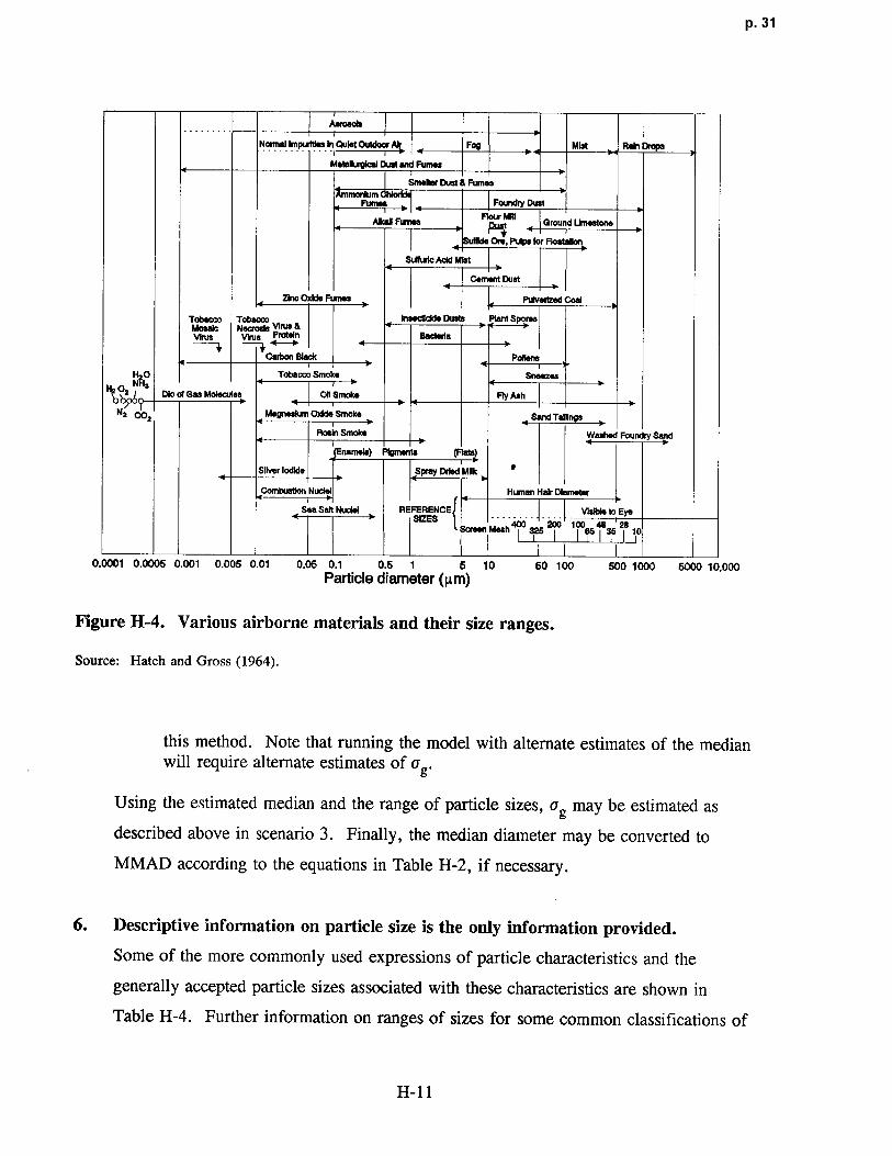
FIgure H-4. Various airborne materials and their size ranges .
Source: Hatch and Gross (1964) .
this method. Note that running the model with alternate estimates of the medianwill require alternate estimates of a g .
Using the estimated median and the range of particle sizes, vg may be estimated as
described above in scenario 3 . Finally, the median diameter may be converted to
MMAD according to the equations in Table H-2, if necessary .
6. Descriptive information on particle size is the only information provided.
Some of the more commonly used expressions of particle characteristics and the
generally accepted particle sizes associated with these characteristics are shown in
Table H-4 . Further information on ranges of sizes for some common classifications of
H-11

p. 32
TABLE H-4 . GENERAL PARTICLE DESCRIPTIONS AND ASSOCIATED SIZE S
Particle Description Size (µm)
Coarse > 2.5
Fine < 2.5
Fumes, Smoke < 1
Fog, Mist < 1 - 20
particles may be found in Figure H-4. Using this information, the median may be
estimated as described in scenario 5, and vg estimated as described in scenario 4 .
7. No information on particle sizes provided.
Studies that do not provide this information should be suspect for deficient quality .
Some of the older toxicology literature may not provide this information, however, and
a default value may need to be invoked . The first approach in this situation is to
attempt an estimate of particle size and distribution based on the generation apparatus
used. Operating specifications of various generation systems are available from the
manufacturer or reviewed elsewhere (Moss and Cheng, 1989 ; American Conference of
Governmental Industrial Hygienists, 1978 ; Willeke, 1980) . In conjunction with this
information, the knowledge that prior to the late 1970s, the generation technology was
not sufficiently sophisticated to deliver consistent exposures of particle sizes above 3 µm
(MMAD) can be used to construct a default approach . The recommended default
approach is to use the MMAD and vg characteristic for the given generation system that
is <3 µm and that yields the smallest (i .e., most conservative) RDDR values for the
respiratory tract region of interest . Knowledge of the measurement range of the
instrument used to characterize the test atmosphere can also be used to estimate a
particle size . Figure H-3 provides the measurement ranges of some aerosol monitoring
instruments .
H-12
p. 33
The second approach is to use particle size information from other studies to estimat e
the particle characteristics for the exposure in question . If no such information is
available, Figure H-4 provides the general size ranges for most common classifications
of particles . Using this information, the median may be estimated as described in
scenario 5, and a9 estimated as described in scenario 4 .
H-13

p. 34
APPENDIX I
DERIVATION OF AN APPROACH TO DETERMINEHUMAN EQUIVALENT CONCENTRATIONS FOR
EFFECTS OF EXPOSURES TO GASESIN CATEGORIES 1 AND 2
As discussed in Sections 3 .2 and 4 .3, the optimal approach to describe regional
respiratory tract dose for extrapolation across species is to use a comprehensive dosimetry
model. The limited number of sophisticated dosimetry models that currently exist are either
chemical-specific or class-specific and require an extensive number of model parameters .
As discussed in Section 3 .2, the chemical-specific or class-specific nature of these models has
been dictated by the physicochemical properties of the subject gases and therefore any single
resultant model is not applicable to the broad range of physicochemical properties of gases
(or vapors-herein referred to as gases) that this methodology is aimed at addressing .
In addition, sufficient data from which to estimate model parameters for each gas are often
unavailable .
A conceptual framework was thus developed to structure mathematical models that
require limited gas-specific parameters and that may be further reduced by simplifying
assumptions to forms requiring minimal information. The models in reduced form are the
basis of the default adjustments used in Section 4 .3 and are used to estimate the human
equivalent concentrations (HECs) from no-observed-adverse-effect levels (NOAELs) of gases
when the lack of data for the required parameters precludes more comprehensive modeling .
This appendix provides the conceptual framework and background details of the default
derivation for the adjustments used in Section 4 .3 .
Because adverse respiratory effects may be observed in the extrathoracic (ET),
tracheobronchial (TB), or pulmonary region (PU), the conceptual framework is constructed to
derive a regional description of dose, defined as the regional absorption rate . The regional
absorption rate is used as a surrogate of regional dose and is assumed to represent th e
I-1

p. 35
effective dose for evaluation of the dose-response relationship . The physicochemical
properties such as the water solubility and reactivity (e .g., ionic dissociation or tissue
metabolism) of the gas in the respiratory system are major determinants of the regional
absorption rate. For example, styrene is relatively insoluble in water and unreactive with the
respiratory tract surface liquid and tissue. This gas is therefore absorbed primarily in the
lung periphery, where it partitions across the blood-gas barrier . Formaldehyde, however, is
both water soluble and reactive such that most of the gas is absorbed in the ET region . The
concept of differentiating gases based on their stability, reactivity, or tissue metabolic activity
has been proposed by Dahl (1990) who presented a methodology to assist in categorizing
gases . As discussed in Section 3 .2, delineation of the categories is accomplished by
identifying dominant mechanistic determinants of absorption that are based on the
physicochemical characteristics of the gases . The dominant mechanistic determinants are
used to construct a conceptual framework that directs development of the dosimetry model
structures .
The categorization scheme discussed in Section 3 .2 and developed more fully herein is
used to establish a dosimetry model structure for three categories of gases from which default
equations are developed by imposing additional simplifying assumptions . Model structures
for two of the three categories are developed in this Appendix. The structure for Category 3
gases is developed in Appendix J . Gases in Category 3 are relatively water insoluble and
unreactive in the ET and TB surface liquid and tissue and thus exposures to these gases result
in a relatively small dose to these regions . The uptake of these gases is predominantly in the
PU region and is perfusion limited . The site of toxicity of these gases is generally remote to
the principal site of absorption in the respiratory tract . Thus, the relatively limited dose to
the ET .and TB regions does not appear to result in any significant ET or TB respiratory
toxicity . Toxicity may, however, be related to recirculation . An example of a Category 3
gas is styrene. Gases that fall in Category 3 are modeled using the structure and default
equations presented in Appendix J .
The methodology developed in this appendix addresses the absorption of gases that are
relatively water soluble and/or reactive in the respiratory tract (Categories 1 and 2 of the
scheme described in Section 3 .2). The focus here is on the description of dose for
respiratory tract effects . This is not to suggest that the toxicity is limited to the respiratory
I-2

p. 36
regions and in fact, for Category 2, the model structure may be used to define a dosimetri c
for remote toxicity because this category of gases has physicochemical characteristics that
may result in some systemic circulation of toxicant . The assumption of this modeling
approach is that the description of an effective dose to each of these regions for evaluation of
respiratory effects must address the absorption or "scrubbing" of a relatively water soluble
and/or reactive gas from the inspired airstream as it travels from the ET region to the PU
region . That is, the dose to the distal regions (TB and PU) is affected by the dose to the
region immediately proximal . The appropriateness of assessing proximal to distal dose
representative of the scrubbing pattern is supported by the often observed proximal to distal
progression pattern of dose-response for respiratory tract toxicity with increasing
concentration . At low concentrations of relatively water soluble and/or reactive gases,
observed effects are isolated to the ET region . At higher concentrations, more severe effects
occur in the ET region and toxicity is also observed to progress to the distal regions . The
intensity or severity of the distal toxicity also progresses with increased exposure
concentrations .
In the following section, the conceptual framework that directs development of
dosimetry models is discussed . The framework is constructed according to the categorization
scheme of gases based on physicochemical characteristics . The physicochemical
characteristics are used to define dominant mechanistic determinants of absorption and
thereby determine the mathematical model structure to describe regional dosimetry . The
model structures developed in the framework rely on models that are currently in use ; a
detailed review of potential structures is presented elsewhere (Ultman, 1988) and some are
incorporated here . Description and derivation of the model structure for each category of gas
follows with the exception of gases that are relatively insoluble in water (Category 3) . The
uptake of Category 3 gases is predominantly perfusion-limited and the dosimetry approach for
these is discussed in Appendix J . Thus, the focus of this appendix is on those gases that are
relatively water soluble and/or reactive in the respiratory tract . It should be noted that the
definition of reactivity includes both the propensity for dissociation as well as the ability to
serve as substrate for metabolism in the respiratory tract . The default equations are derived
after the development of the modeling structure for gases in Categories 1 and 2 . These
equations result from the application of further simplifying assumptions necessary to reduce
1-3
p. 37
the required parameters to perform the dosimetry adjustment when minimal data are
available .
I .1 Conceptual Framework
Extrapolation of the dose-response relationship from laboratory animals to humans is
performed based on the absorption in the three respiratory tract regions as defined in
Chapter 3: extrathoracic (ET), tracheobronchial (TB), and pulmonary (PU) . Although toxic
effects may sometimes be observed in a more local area within those regions (e .g., the
olfactory epithelium of the ET region), the parameters required to further subdivide the
description of dose within these regions are not available currently. Several active areas of
investigation, such as the evaluation of regional mass transpoft within the nasal cavity to
create maps of localized flows in rats and monkeys (Kimbell et al ., 1993), of regional mass
transport in the human (Lou, 1993), and of metabolic activity of localized tissues in rodents
(Bogdanffy et al., 1986, 1987, 1991 ; Bogdanffy and Taylor, 1993 ; Kuykendall et al ., 1993),
are anticipated to provide the data required to estimate the necessary parameters on a species-
specific basis .
The conceptual framework used to direct development of model structures for estimation
of regional gas dose is based on the categorization scheme presented in Section 3 .2.2. This
categorization scheme is based on the physicochemical characteristics of water solubility and
reactivity as shown in Figure I-1 . These characteristics are used to define dominant
mechanistic determinants of absorption and thereby direct development of model structures .
As will be described, the modeling structure favored for this development has been used
extensively to quantify gas exchange or absorption of pollutants . This structure is in no way
promoted exclusively as the only one available ; it is however used here to develop the
approach for dosimetric adjustment . Its application to each category will be presented and
the default equations for use with limited parameters will be derived .
I.1 .1 Category Scheme for Gases with Respiratory Effect s
This appendix focuses on those gases that are relatively water soluble and/or reactive in
the respiratory tract (i .e., those gases in Categories 1 and 2, initially defined in Section 3 .2) .
I-4
p. 38
• • • • ••• ~~ • • • 1
• ••• • ~ • ••
• • • • ••00 0
• ' a ' •'•'' • • • • • ~~ •.0 • •
' ' ' '':0000 0' • • • •
iott
•' •• • ' ' •
• • • • • • • ' '
•• • • •
• • • • • •• • •
' • • • •
Reactivity jGas Category Scheme Location
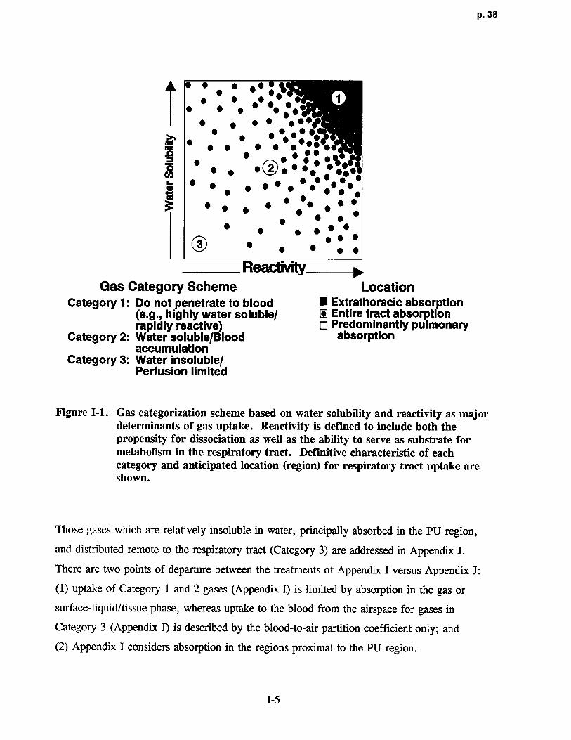
Category 1 : Do not penetrate to blood ■ Extrathoracic absorption(e.g., highly water soluble/ © Entire tract absorptionrapidlyreactive) O Predominantly pulmonary
Category 2 : Water soluble/Blood absorptionaccumulation
Category 3: Water insoluble/Perfusion limited
Figure I-1 . Gas categorization scheme based on water solubility and reactivity as majordeterminants of gas uptake. Reactivity is defined to include both thepropensity for dissociation as well as the ability to serve as substrate formetabolism in the respiratory tract. Definitive characteristic of eachcategory and anticipated location (region) for respiratory tract uptake areshown.
Those gases which are relatively insoluble in water, principally absorbed in the PU region,
and distributed remote to the respiratory tract (Category 3) are addressed in Appendix J .
There are two points of departure between the treatments of Appendix I versus Appendix J :
(1) uptake of Category 1 and 2 gases (Appendix I) is limited by absorption in the gas or
surface-liquid/tissue phase, whereas uptake to the blood from the airspace for gases in
Category 3 (Appendix J) is described by the blood-to-air partition coefficient only ; and
(2) Appendix I considers absorption in the regions proximal to the PU region .
I-5
p. 39
Two categories of gases with potential respiratory effects at the uptake site have been
identified for simplifying the methods for dose determination . The categories separate the
gases on the basis of the physicochemical absorption parameters and the consequent dominant
determinants of absorption . The two categories of gases with potential respiratory effects are
(1) highly water soluble and/or rapidly irreversible reactive gases ; and (2) water soluble gases
and gases that may also be rapidly reversibly reactive or moderately to slowly irreversibly
metabolized in respiratory tract tissue .
The gases in Category 1, highly water soluble and rapidly irreversibly reactive, are
distinguished by the lack of a blood-phase component to the transport resistance (i .e., almost
none of the gas reaches the bloodstream), which allows the overall transport to be described
by the transport resistance through air and liquid/tissue phases only (i .e., the two-phase
transport resistance model) . Examples of gases in this category are hydrogen fluoride,
chlorine, formaldehyde, and the volatile organic acids and esters .
Gases in Category 2 are distinguished from those in Category 1 by the potential for
accumulation of a significant blood concentration that could reduce the concentration gradient
driving the absorption process and thereby reduce the regional absorption rate . In addition,
the accumulated blood or surface liquid/tissue concentration may impose a backpressure (i .e.,
a significant reverse in the concentration gradient) during exhalation which could result in
desorption . Category 2 gases may be further subdivided by distinguishing between those that
react reversibly with the surface liquid or underlying tissue from those that react irreversibly .
A gas that is moderately to slowly irreversibly metabolized in the respiratory tract will
effectively reduce tissue concentration and thereby increase the concentration gradient during
absorption and decrease it during desorption . In contrast, reversible reactions will not affect
the gradient dramatically . Consequently, in the case of irreversible reactions, the reaction
rate may need to be included in the model . In the case of Category 2 gases undergoing a
reversible reaction, the reaction may be incorporated into the model by the use of an
enhanced solubility term . Examples of Category 2 gases are ozone, sulfur dioxide, xylene,
propanol, and isoamyl alcohol .
General physicochemical properties of the gases have been used to delineate each of the
categories . The boundaries between categories are not definitive . Some compounds may
appear to be defined by either Category 1 or Category 2 because water solubility an d
1-6

p. 40
reactivity are a continuum . Thus, although sulfur dioxide is reversibly reactive, which would
categorize it as a Category 2 gas, it is also highly soluble such as to be a Category 1 gas .
Similarly, ozone is highly reactive yet only moderately water soluble . More explicit
delineation of the categories will be made upon review of the empirical data and the
predictability of the model structures for gases that may appear to fit more than one category .
The modeling approach for the determination of dose for each of these categories of gases is
discussed separately in the following sections, along with the determination of the default
methods if sufficient detail from which to determine dose is not available for a specific gas .
1.1 .2 General Model Structure
Numerous model structures have been used to describe toxicant uptake in the respiratory
tract . The structures range from compartmental models, such as physiologically based
pharmacokinetic (PBPK) models in which spatial details are ignored, to distributed parameter
models, such as the finite difference models of McJilton et al . (1972) and Miller et al .
(1985) . The finite difference models have been applied to specific gases, but a generalized
structure was developed by Hanna et al . (1989) for water soluble gases . Several reviews of
the various structures are available (Morgan and Frank, 1977 ; Ultman, 1988, 1994) .
Methodologies to describe respiratory uptake of gases have been successfully applied by
using two types of empirical compartmental models . These models are distinguished by the
gases to which they have been applied . The ventilation-perfusion model first applied to the
exchange of carbon dioxide/oxygen (C02/02) in the lung periphery has been principally and
most successfully employed to describe the stable and less soluble gases . The modeling of
the respiratory tract using the ventilation-perfusion model has become a central component of
PBPK models as described in Appendix J (Ramsey and Andersen, 1984 ; Andersen et al .,
1987a; Overton, 1989 ; Andersen et al ., 1991) . In a ventilation-perfusion model (or Bohr
model), the mass of inhaled chemical reaching the lung periphery, or PU region, is calculated
as the product of the ambient concentration and the alveolar ventilation rate . The
ventilation-perfusion model would overpredict the gas concentration that reaches the alveoli if
the gas is absorbed or reacts with the ET and TB airway surface liquid and/or tissue .
The second type of model was developed to describe the fraction of an absorbing or
reacting gas that penetrates the ET region . This model, which will be referred to as the
I-7

p. 41
penetration fraction model, was first used by Aharonson et al . (1974) to demonstrate
empirically the different upper airway absorption efficiencies for gases with differing
physicochemical properties . This modeling concept has since been utilized by Kleinman
(1984), Morgan and Frank (1977), Ultman (1988), Hanna et al . (1989), Gerde and Dahl
(1991), and Morris and Blanchard (1992) . A principal focus of these modeling efforts has
been to predict the scrubbing efficiency of the ET airway based on the ventilation rate and the
physicochemical properties of the gas. However, the general applicability of the penetration
model has often been limited by the assumption that the gas blood concentration approaches
zero, thereby requiring complete systemic elimination . Retaining the blood concentration in
the model allows greater flexibility for inclusion of the reduction in the concentration
gradient, which would reduce the absorption rate if the gas were to accumulate in blood .
In this conceptual framework, the methodology to adjust regional respiratory dose from
laboratory animals to humans for evaluation of respiratory tract effects is achieved for the
relatively water soluble and/or reactive gases (Categories 1 and 2) by integrating the above
two types of empirical models . These models have been used extensively and are therefore
favored due to their wide use and potential for empirical measurement of model parameters .
The penetration fraction model provides estimation of the ET and TB doses . These are used
to adjust the mass of inhaled gas reaching the PU region in the ventilation-perfusion model .
Additional systemic compartments (e .g., liver and fat) may be required in the model to
describe gases that accumulate significantly in the blood . The addition results in a model
structure similar to PBPK models; however, it also incorporates the mass transport
description of the scrubbing of the gas in the ET and TB regions .
The approach herein to determine the regional dose within the respiratory tract is
developed by relying on the overall mass transport coefficient, Kg, to characterize the
transport of gases between the airphase, the intervening surface liquid and tissue, and the
blood . In the absence of empiric measurement, Kg may be estimated or scaled for a given
gas based on its physicochemical properties and reactivity within the respiratory tract. In the
following section, a derivation of Kg is provided and the influence of gas physicochemical
characteristics on Kg is discussed . The definitions of parameter symbols used in the
following sections are provided in Table I-1 .
1-8

p. 42
TABLE I-1. DEFINITION OF PARAMETER SYMBOLS USED IN APPENDIX I
a Airway perimeter (cm)
Co Initial concentration (mg/cm3)
C.1„ Pulmonary region gas concentration (mg/cm')
Ca(x) Gas concentration as a function of x(mg/cm3)
Cb Blood concentration (mg/cm3)
C~1B Gas concentration in equilibrium with blood concentration (mg/cm3)
CWr Concentration of gas in its chemically transformed (reacted) state (mg/cm)
Cf Concentration in the fat compartment (mg/cm3)
Cg Gas phase concentration in airway lumen (mg/cm)
Cg; Gas-phase concentration at the interface of the gas phase with the surface-liquid/tissue phase(mg/cm)
C; Inhaled concentration (mg/cm3)
Cl Surface-liquid/tissue phase concentration (mg/cm3)
CL, Concentration in the lung compartment (mg/cm)
CU8 Surface-liquid/tissue concentration in equilibrium with the gas phase (mg/m)
Cl; Surface-liquid/tissue concentration at the interface of the gas phase and thesurface-liquid/tissue phase (mg/cm3 )
CS Imposed concentration (mg/cm)
CT/A Concentration of reacted and unreacted gas in arterial blood (mg/cm)
CTN Concentration of reacted and unreacted gas in venous blood (mg/cm)
CZ Concentration in the surface-liquid/tissue phase (mg/cm3 )
CA Arterial (unoxygenated) blood concentration (mg/cm3)
CLfa, Clearance from the fat compartment (cmZ/min)
CLLn, Clearance from the liver compartment (cm2/min)
CLSYS Clearance from the systemic compartment (cmZ/min)
CV Concentration in venous (oxygenated) blood entering gas-exchange (PU) region (mg/cm)
CX(EXH),, Concentration exiting from extrathoracic region on exhalation (mg/cm)
CX(EXH)PU Concentration exiting from pulmonary region upon exhalation (mg/cm3)
CX(EXH)TB Concentration exiting from tracheobronchial region upon exhalation (mg/cm)
CX(INH),, Concentration exiting from extrathoracic region upon inhalation (mg/cm)
CX(INH)TB Concentration exiting from tracheobronchial region upon inhalation (mg/cm)
D Deposited fraction of mass (unitless)
DI Liquid diffusivity (cmZ/min )
dx Differential of axial distance into airway (cm )
dy Differential of axial distance into capillary segment (cm)
dz Differential of distance into the surface-liquid/tissue phase (cm)
E" Elimination rate in the lung compartment (cmZ/min)
EMAx Maximum extraction efficiency (unitless)
1-9
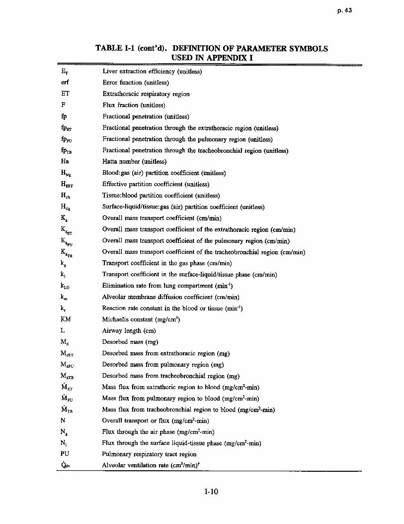
p. 43
TABLE I-1 (cont'd) . DEFINITION OF PARAMETER SYMBOLSUSED IN APPENDIX I
ET Liver extraction efficiency (unitless)
erf Error function (unitless)
ET Extrathoracic respiratory region
F Flux fraction (unitless)
fp Fractional penetration (unitless )
fpEr Fractional penetration through the extrathoracic region (unitless)
fppU Fractional penetration through the pulmonary region (unitless)
fpTB Fractional penetration through the tracheobronchial region (unitless)
Ha Hatta number (unitless)
Ha8 Blood:gas (air) partition coefficient (unitless)
HEFF Effective partition coefficient (unitless)
H,~b Tissue :blood partition coefficient (unitless)
Ht/9 Surface-liquid/tissue:gas (air) partition coefficient (unitless)
Kg Overall mass transport coefficient (cm/min)
KgEr Overall mass transport coefficient of the extrathoracic region (cm/min)
K9PU
Overall mass transport coefficient of the pulmonary region (cm/min)
K&rB Overall mass transport coefficient of the tracheobronchial region (cm/min)
kg Transport coefficient in the gas phase (cm/min)
k , Transport coefficient in the surface-liquid/tissue phase (cm/min)
kLG Elimination rate from lung compartment (min-)
k. Alveolar membrane diffusion coefficient (cm/min)
k, Reaction rate constant in the blood or tissue (min-')
KM Michaelis constant (mg/cm)
L Airway length (cm)
Ma Desorbed mass (mg)
MdEr Desorbed mass from extrathoracic region (mg)
MdpU Desorbed mass from pulmonary region (mg)
M(rrB Desorbed mass from tracheobronchial region (mg)
1VI,r Mass flux from extrathoric region to blood (mg/cm2-min)
IVIpU Mass flux from pulmonary region to blood (mg/cm2-min )
IVITB Mass flux from tracheobronchial region to blood (mg/cm2-min)
N Overall transport or flux (mg/cm2-min )
Ng Flux through the air phase (mg/cm2-min)
N , Flux through the surface liquid-tissue phase (mg/cm2-min)
PU Pulmonary respiratory tract region
41V Alveolar ventilation rate (cm3/min)t
I-10

p. 44
TABLE I-1 (cont'd). DEFINITION OF PARAMETER SYMBOLSUSED IN APPENDIX I
Qb Local blood flow rate (cm3/min) t
Qr Cardiac output (cm3/min) t
RGD Regional gas dose (mg/cmZ-min )
RGDREr Regional gas dose ratio for the extrathoracic region (unitless)
RGDRPU Regional gas dose ratio for the pulmonary region (unitless)
RGDRTB Regional gas dose ratio for the tracheobronchial region (unitless)
SA Surface area of unspecified respiratory region (cmz)
SAEr Surface area of the extrathoracic region (cm)
SATB Surface area of the tracheobronchial region (cm)
SAPU Surface area of the pulmonary region (cm)
Sp Blood perfusion surface area (cm)
t Time (min)
tEXH Time (duration) of exhalation (min )
TB Tracheobronchial respiratory tract region
V Volumetric flow rate (mg/min)
Vb Capillary blood volume (cm3)
VLG Lung compartment volume (cm3)
VMAX Maximum velocity of saturable (Michaelis-Menton) metabolism path (mg/cmz-min)
VE Minute volume (cm3/min) t
x Distance into the airway (cm)
Ay Thickness of the surface liquid-tissue layer (cm)
z Distance into the surface-liquid/tissue phase (cm)
Az Surface-liquid/tissue phase thickness (cm )
t I mL = 1 cm3, so cm3/mm = mL/min .Also note that concentrations are expressed as mg/cm3 (1 mg/cm3 = 10 " mg/m3) .
1 .1.3 Overall Mass Transport Coefficien t
The concept of the overall mass transport coefficient is based on a concentration
gradient analysis similar to Fick's Law of Diffusion and is utilized to describe transport
through several different phases such as air and liquid. The structure of the two-phase mass
transport resistance model simplifies the description of mass transport to a minimal number of
parameters that may be scaled to gases differing in their physicochemical properties as
described later . The more definitive evaluation of transport is to describe absorption by a
I-11
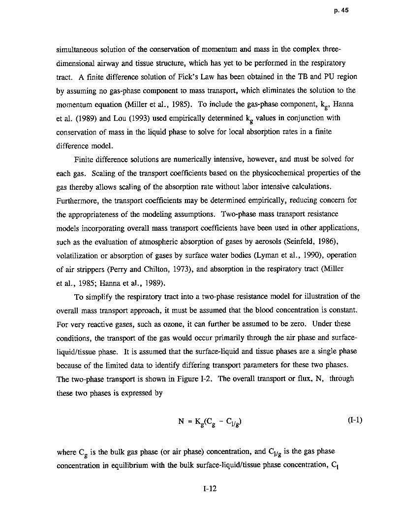
p. 45
simultaneous solution of the conservation of momentum and mass in the complex three-
dimensional airway and tissue structure, which has yet to be performed in the respiratory
tract . A finite difference solution of Fick's Law has been obtained in the TB and PU region
by assuming no gas-phase component to mass transport, which eliminates the solution to the
momentum equation (Miller et al ., 1985) . To include the gas-phase component, kg, Hanna
et al . (1989) and Lou (1993) used empirically determined kg values in conjunction with
conservation of mass in the liquid phase to solve for local absorption rates in a finite
difference model .
Finite difference solutions are numerically intensive, however, and must be solved for
each gas . Scaling of the transport coefficients based on the physicochemical properties of the
gas thereby allows scaling of the absorption rate without labor intensive calculations .
Furthermore, the transport coefficients may be determined empirically, reducing concern for
the appropriateness of the modeling assumptions . Two-phase mass transport resistance
models incorporating overall mass transport coefficients have been used in other applications,
such as the evaluation of atmospheric absorption of gases by aerosols (Seinfeld, 1986),
volatilization or absorption of gases by surface water bodies (Lyman et al ., 1990), operation
of air strippers (Perry and Chilton, 1973), and absorption in the respiratory tract (Mille r
et al., 1985 ; Hanna et al ., 1989) .
To simplify the respiratory tract into a two-phase resistance model for illustration of the
overall mass transport approach, it must be assumed that the blood concentration is constant .
For very reactive gases, such as ozone, it can further be assumed to be zero . Under these
conditions, the transport of the gas would occur primarily through the air phase and surface-
liquid/tissue phase . It is assumed that the surface-liquid and tissue phases are a single phase
because of the limited data to identify differing transport parameters for these two phases .
The two-phase transport is shown in Figure 1-2 . The overall transport or flux, N, through
these two phases is expressed by
N = Kg(Cg - Cl lg) (I-1)
where Cg is the bulk gas phase (or air phase) concentration, and Ci /g is the gas phase
concentration in equilibrium with the bulk surface-liquid/tissue phase concentration, C l
1-12

p. 46
00"
Airway Lumen4~~x
Gas Phase Surface-Liquid / Tissue Phase Blood
~---- -~
Distance FromInterface
Cg
Cgi
Cli
tC
1\ kr
~` .
'Cl= Cb=
0
A Z
Air Phase =1 Surface
Resistance ~- f N'qeometry) Liquid-Tissue = H 1 = f(k~, D, A Z)Resistance Vg ~
FlIgure 1-2. Schematic of two-phase mass transport resistance model . The definitionsfor the parameter symbols are provided in Table I-1 .
1-13

p. 47
(Perry and Chilton, 1973), such that Cl/g is .equal to the ratio of the surface-liquid/tissue
concentration, C1, to the gas partition coefficient, Ht/g .
The overall mass transport coefficient may be determined from the transport coefficients
of each individual phase . It is obtained by considering the flux through each phase (Perry
and Chilton, 1973) such that
Ng = kg(Cg - Cgi) (1-2)
where Ng is the flux through the air phase, kg is the transport coefficient in the gas phase,
and Cgi is the gas-phase concentration at the interface of the gas phase and the surface-liquid
tissue phase, and
Nl = k1(Cli - C) (1-3)
where Nl is the flux through the surface liquid-tissue phase, kl is the transport coefficient in
the surface-liquid/tissue phase, and Cli is the surface-liquid/tissue concentration at the
interface of the gas phase and the surface-liquid/tissue phase .
Steady state (or quasi-steady state as occurs in the respiratory tract during inhalation or
exhalation) requires the following condition :
N = Ng = N1, (1-4)
or
N = Kg(Cg - Cl1g) = kg(Cg - Cgi) = k1(Cli - C)• (1-5)
In the two-phase resistance approach defined by Equation I-5 above, the overall mass
transport resistance is defined by the reciprocal of the mass transport coefficient, 1/Kg, and is
composed of the resistance to lateral movement of the absorbing gas through the air an d
I-14

p. 48
through the liquid and tissue as shown in Figure 1-2 . The resistance in series can be derived
from Equation 1-5 as
1 _ 1 + 1 (1-6)Kg kg Ht/gk1
In the case where the surface liquid and tissue cannot be assumed to be a single compartment,
a separate partition coefficient and transport coefficient would need to be incorporated into
Equation 1-6 .
The definition of the overall mass transport coefficient provided in Equation 1-6 may be
used to evaluate the conditions in which a single phase, either gas phase or surface-
liquid/tissue phase, determines the overall mass transport coefficient . To demonstrate
predominance of a single phase, it is further assumed that blood flow does not contribute to
the overall mass transport coefficient (i .e., that there is no accumulation in blood). In the
case of a reactive gas and/or a gas relatively soluble in both the tissue and blood, the
transport resistance through the gas phase, 1/kg, may be greater than the transport resistance
in the other phases (i .e., kg << Ht/gkl) such that
1 /Kg - Mg. (1-7)
The gas phase term, kg, is dependent on flow rate, flow geometry, and the gas phase
diffusivity . In cross-species comparisons, the flow geometry differences of the species are
likely to predominately determine kg . Additionally, recent data found that kg differed
significantly between living subject geometry and cadaver geometry so that it is reasonable to
expect geometry to affect interspecies differences (Lou, 1993) .
Liquid phase controlled absorption (i .e., Ht/gkl << kg) is typically identified by a gas
of moderate to low water solubility and low reactivity . In the case of a nonreactive gas,
Ht/gkl may be approximated by the surface-liquid/tissue :gas partition coefficient, the liquid
diffusivity (D) , and the thickness of the liquid-tissue layer (Ay), such tha t
1-15

p. 49
Ht/gk1 1~9 1Ht/g • (1-8)Y
For reactive gases, kl would need to be evaluated to include the transformation rate (Bir d
et al ., 1960 ; Perry and Chilton, 1973 ; Ultman, 1988) . However, as the reactivity increases,
it is less likely that the absorption rate will remain liquid phase controlled due to the
increasing influence of the gas phase . In the case of a liquid-controlled absorption process,
Ht/gkl may be substituted for kg in Equation 1-7 .
As discussed, each of the transport coefficients is dependent on the transport properties
of the gas within the respective phase that alter the concentration gradient indicated in
Figure I-1 . Thus, in the case of the gas phase mass transport coefficient, kg, the mass
transport is affected by the flow rate (ventilation rate), the gas phase diffusivity, and the loca l
(regional) airway geometry . The dependence of kg on these parameters is discussed in
greater detail by Hanna et al . (1989) and Lou (1993) . The surface-liquid/tissue phase
transport coefficient is determined by the phase thickness (&z), the liquid phase diffusivity,
and the reactivity (e.g., ionic dissociation and metabolism) in the surface-liquid/tissue . The
dependence of kl on these parameters is discussed in greater detail by Ultman (1988) .
The penetration fraction model may be used to empirically determine the overall mass
transport coefficient (Section I .2.1), provided the fractional penetration, fp, is measured .
Because fp is both gas and species specific, the Kg value will similarly be gas and species
specific . However, data for fp and Kg specific to a gas or gases may be used in a predictive
fashion by scaling to the physicochemical properties of solubility, diffusivity, and reactivity .
Using values of Kg obtained in a single species, Kg can be scaled within the species for
a different gas by decomposing Kg to the individual transport resistances (i .e., the gas phase
and surface-liquid/tissue phase mass transport coefficient) . In humans, empirical measures of
kg have been obtained in casts of the human nasal cavity (Nuckols, 1981 ; Hanna and Scherer,
1986; Lou, 1993) and can be used to decompose Kg . Although kg is species specific, it may
be scaled to other gases by scaling to the gas diffusivity (Hanna et al ., 1989) . Therefore, for
a gas in which kg << Ht/gkl, this scaling may be sufficient to predict fp and dose . Similar
scaling using the diffusivity and reactivity of a gas for which fp is unknown may be
performed for the surface-liquid/tissue phase transport coefficient, kl . For gases in which the
1-16

p. 50
prediction of Kg, and therefore fp, depends on the surface-liquid/tissue phase, the solubilit y
and reactivity of the gas must also be used in the scaling (Equation 1-6) .
A difficulty arises due to the lack of kg values in airways of laboratory animals .
Decomposition of an empirically determined Kg to the individual components must therefore
be made based on a data base in which Ht/gkl may be determined . An approach is under
development to obtain data from several gases to decompose Kg into each component and
perform an evaluation of kg for gases in each category to obtain a measure of consistency
within a species . This effort is underway and will be published as a technical support
document to this publication .
Absorption within the respiratory tract cannot always be assumed to be modeled by a
two-phase transport resistance model ignoring the blood concentration. In cases where the
absorption in the blood contributes to overall absorption, additional mass transport resistances
must be considered . Accumulation in the bloodstream may reduce the concentration driving
force (and thereby reduce the absorption rate) as well as contribute to the development of a
back pressure, which may result in desorption during exhalation due to the reversal in the
concentration gradient between the air and tissue . Gases that are likely to exhibit these
characteristics are Category 2 gases that are water soluble and rapidly reversibly reactive or
those that are moderately to slowly irreversibly metabolized in the respiratory tract,
previously referred to as "transition gases" (Dahl, 1990) . The contribution of the blood to
both the overall mass transport resistance and to the potential for desorption during exhalation
was considered in the categorization of gases based on their physicochemical properties . The
categorization of gases with respiratory effects is used as the basis for defining the model
structure and, in particular, the overall mass transport coefficient .
1.2 MODEL FOR CATEGORY 1 GASES
Category 1 gases are defined as gases that are highly water soluble and/or that may
react rapidly and irreversibly in the surface liquid and tissue of the respiratory tract . Due to
these physicochemical characteristics, these gases are distinguished by the property that a
significant back pressure from the surface-liquid/tissue phase during exhalation does not
develop. A back pressure resulting from the reversal in the concentration gradient betwee n
1-17
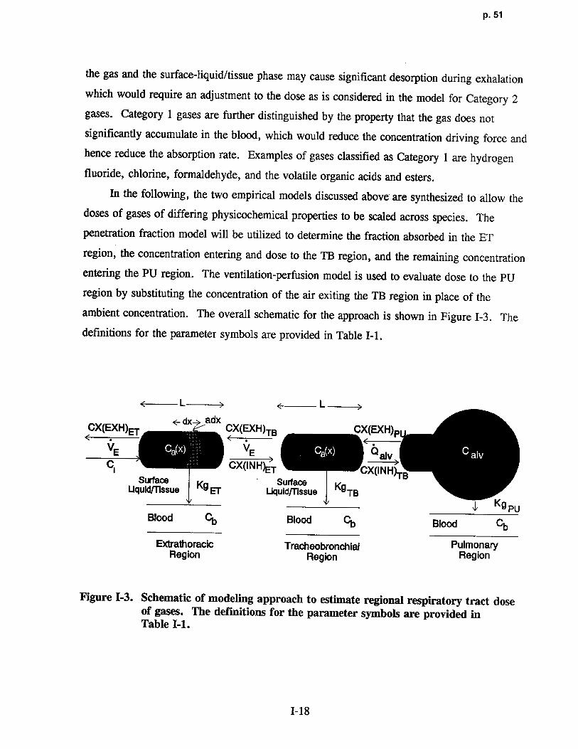
p. 5 1
the gas and the surface-liquid/tissue phase may cause significant desorption during exhalation
which would require an adjustment to the dose as is considered in the model for Category 2
gases . Category 1 gases are further distinguished by the property that the gas does not
significantly accumulate in the blood, which would reduce the concentration driving force and
hence reduce the absorption rate . Examples of gases classified as Category 1 are hydrogen
fluoride, chlorine, formaldehyde, and the volatile organic acids and esters .
In the following, the two empirical models discussed above are synthesized to allow the
doses of gases of differing physicochemical properties to be scaled across species . The
penetration fraction model will be utilized to determine the fraction absorbed in the ET
region, the concentration entering and dose to the TB region, and the remaining concentrationentering the PU region. The ventilation-perfusion model is used to evaluate dose to the PU
region by substituting the concentration of the air exiting the TB region in place of the
ambient concentration . The overall schematic for the approach is shown in Figure 1-3 . The
definitions for the parameter symbols are provided in Table I-1 .
< - L> < L >
CX(EXH) E- dX~ adx CX EXH` ( )TB CX(EXH)PVE VE ~~
Ci CX(I~NH)ET CX(INH)TBSurface Surface Kg
Uquid/Tissue Kg ET Liquid~ssue TBy Kg PU
Blood Cb Blood Cb Blood Cb
Extrathoracic Tracheobronchial PulmonaryRegion Region Region
Figure 1-3. Schematic of modeling approach to estimate regional respiratory tract doseof gases. The definitions for the parameter symbols are provided inTable I-1 .
1-18

p. 52
1.2 .1 Extrathoracic Region: The Penetration Fraction Model
The penetration fraction model, designed to evaluate the upper airway scrubbing
efficiency, is based on a mass .-balance approach . The change in mass traversing the gas
phase of the extrathoracic region is balanced by the mass absorbed at the gas-liquid interface
of the airway. This balance is written a s
V da _KgEr a(Cl-
Cb/g) (1-9)
where V is the volumetric flow rate; dCg/dx is the rate of change of the airstream
concentration (gas phase) as a function of distance into the airway, x ; KgET is the overall
mass transport coefficient between the airstream and the blood in the ET region ; a is the local
airway perimeter; Ci is the inspired gas concentration ; and Cb/g is the gas concentration that
would be in equilibrium with the blood concentration . Cb/g is equal to the ratio of the blood
concentration, Cb, to the blood:gas (air) partition coefficient, Hb/g .
To evaluate . the change in concentration over the length of the ET region, Equation 1-9
is integrated resulting in the following relationship :
-KB~aL
(CX(INH)ET_Cb/g) (1-10)e ,
(Ci-Cb/g)
where CX(INH)ET is the gas concentration exiting the ET region and L is the length of the
airway such that the product of a and L is the surface area of the ET region, SAET•
Equation I-10 indicates that CX(INH)ET will equal Ci at an infinite volumetric flow rate .
In the case of Category 1 gases/vapors, CX(INH)ET and Ci are much greater than Cb/g,
so that Equation 1-10 can be further reduced to
-Kg~ SA~
CX(INH)ETfPET Ci e
1-19

p. 53
where fpET is the penetration fraction through the ET region and is given as the ratio of the
gas concentration exiting the region, CX(INH)ET, to the gas concentration entering the
airway, Ci. The relationship shown in Equation I-11 suggests that the product of the overall
mass transport coefficient and the surface area may be obtained by plotting fpET as a function
of volumetric flow rate . Indeed, many investigators have used this method to present
empirical results (Aharonson et al ., 1974; Kleinman, 1984 ; Morris and Blanchard, 1992) .
As an example, provided that SAET is known, Equation I-11 may be used to evaluate KgET,
in the form of
1 ln PET = - Kg~.SAET V , (1-12)
where KgETSAET is the slope if the relationship between In fpET and 1/ V is linear .
Equation 1-12 is similar to the relationship developed by Morris and Blanchard (1992) .
Morris and Blanchard chose to fit D/fpET to l/V, where D is the deposited fraction, 1-fpET .Using Equation 1-12 in conjunction with a power series expansion of the exponential term of
Equation I-11 results in
D KgFrSAET
(1-13)fPET V
It should be noted, however, that plotting either In fpET or D/fpET against 1/ V may not
be linear. The nonlinearity was first reported by Aharonson et al . (1974) . Both Ultman
(1988) and Hanna et al . (1989) attribute the nonlinearity to the contribution of the gas phase
mass transport coefficient, kg, to the overall transport rate . Thus, Kg is a function o f
V when affected by kg, thereby producing the nonlinearity .
Equation 1-6 may be used to evaluate KgET if sufficient information is available to
calculate the individual mass transport coefficient for each phase . Empirical determinations
of KgET may also be obtained from Equation 1-12 . Furthermore, in the case of gas phase
controlled absorption (i .e., in the case of Category 1 gases) where KgET = kgET 1
Equation 1-12 can be used to evaluate the gas phase mass transport coefficient (kg) for each
species .
1-20

p. 54
To evaluate kg for a single species, empirical measures of the fractional penetration of a
gas in which the gas phase contributes to (or controls) the overall mass transport resistance
must have been determined empirically . The fractional penetration obtained at several flow
rates may be used to evaluate kg from the following relationship, which is obtained by
combining Equations 1-12 and 1-6 such that
-In fpET - ( V 1 + 1 ) • (1-14)SAET kg Ht-/gkl
The value of kg and its functional dependence on V is determined by curve fitting the
empirically determined fpET and V, provided that Ht/g and kl are known . In the case of a
nonreactive gas, kl may be simply estimated . Methods are also available to estimate kl for
reactive gases (Ultman, 1988) . It should be noted that kg will differ among gases and tha t
kg is a function of ventilation rate . Therefore, kg must be scaled by the gas phase diffusivity .
The ventilation dependence of kg allows the two terms, gas phase and surface-liquid/tissue
phase, to be separated. Thus, kg may be evaluated from data of fpET of several gases to
obtain a reasonable estimate of kg in a single species, particularly for the rat, for which
empirical data are most available . Values of kg in other species may also be obtained from
published uptake data (Morris and Smith, 1982 ; Stott and McKenna, 1984 ; Morris et al .,
1986, 1991 ; Morris and Cavanagh, 1987 ; Morris, 1990; Dahl et al ., 1991b ; Bogdanffy
et al ., 1991 ; Morris and Blanchard, 1992 ; Bogdanffy and Taylor, 1993 ; Kuykendall et al .,
1993) .
By using the heat and mass transfer analogy, measures of change in inspired
temperature may be used to obtain an independent estimate of kg (Hanna et al ., 1989) . The
mass transport coefficient, kg, has also already been determined in human casts based on both
mass transport studies (Hanna et al ., 1989 ; Lou, 1993) and heat transport studies (Nuckols,
1981) from which kg is directly calculated .
If the absorption is gas phase controlled (i .e., absorption is completely determined by
transport through the gas phase), Equation 1-12 may be used to determine the gas phase mass
transport coefficient for a single species such that
1-21

p. 55
k -V In fpET (1-15)g SAET
where kg is substituted for Kg . Because kg is a function of flow rate, a plot of In fpETagainst 1/ V will be nonlinear . The nonlinearity determined from empi rical data of a gas
phase controlled absorption process can be used to evaluate the flow rate dependence of kg .
The flow rate dependence is of the form Vn where n is typically between 0 .5 to 0 .8 (Hannaet al., 1989). Note also that kg can not be determined if there is no penetration (i .e. ,
fpET = 0) because in fpET is undefined . The value of kg at a specific flow rate and in a
single species should be relatively constant, changing only slightly as a function of the gas
diffusivity . Using values for kg determined in humans and in a laboratory an imal species
allows the scaling for dose in gas phase controlled absorption (i .e., where kg << Ht/gkl) .
In the case of surface-liquid/tissue phase contro lled absorption, where Kg = Ht/gkl, the
value will be chemical-specific due to the dependence of Ht/gki on solubility and reactivity .Under these circumst ances, Ht/gkl would replace kg in Equation 1-14. The regression of
In fpR to 1/ V would be linear provided that the reactivity is not saturable . Michaelis-Menton
kinetics can be used to define kl and incorporate saturation kinetics which may introduce a
nonlinearity . However, saturation kinetics may be better described by the model for
Category 2 gases in which there may be a significant accumulation in blood thereby reducing
the absorption concentration gradient du ring inhalation, as well as a potential reversal of the
concentration gradient, which would result in desorption du ring exhalation.
The rate of mass absorbed at the gas-surface interface of the airway in a region is
simply the product of the absorbed fraction, 1-fpET, and the total mass inhaled during a
single breath, VCi. With this knowledge, a suitable met ric of dose must now be chosen .
If dose were to be defined on a mass per volume basis, it would implicitly assume that the
outcome would be determined by concentration (i .e., mass/volume) . This assumption would
therefore argue that the most approp riate definition of dose should be one defined on the basis
of surface area (i .e., the mass flux, or dose, defined as mass per surface area-time) . The
mass flux implies a concentration gradient in the tissue such that the localized concentration
would be highest at the surface . The mass flux is thereby a more accurate predictor of the
peak localized concentration and will be used to define dose for this application . The
1-22

p. 56
regional gas dose (RGD), defined as the mass absorbed per surface area per minute (mg/cm2-
min), to the extrathoracic region (ET) is given by
2 CiVRGDET (mass )cm - min) _ (1 - fpET) . (1-16)SAET
From Equation I-11, the regional gas dose to the ET may also be expressed as
-KgEr
SAET
RGDET (1- e E ) (1-17)
ET SAET
The dose expressed in Equation 1-17 is applicable to any animal species provided the
appropriate parameters of that species are used in the assessment . For example, because the
purpose of this appendix is to address extrapolation of respiratory effects from experimental
animal species to humans, the minute volume (VE) is used as the default volumetric flow rate
in the remainder of the derivations because it approximates the flow rate at which the animal
was breathing during the experimental exposure . Further justification of the use of minute
volume is the relatively little desorption that occurs during exhalation, a requirement by
definition of Category 1 gases, suggesting that the dose should be averaged over the entire
cycle. The default values for surface area and minute volume for the various species are
provided in Chapter 4 .
The regional gas dose ratio for the extrathoracic region (RGDRET) of differing species
used to calculate NOAEL(HEC) can also be developed using Equation 1-17 . A comparison
between humans and an experimental test species would result in the following regional gas
dose ratio (RDGR) :
-KgEr
SA r
(CiVE
- eVE
)ARGDRET -
(RGDET)A SA_ ET (1-18)(RGDET)H -Kg,rSAr '
(
CiVE)HO - e VE )HSAE
T
1-23

p. 57
where the subscript A and H refer to values for laboratory animals and humans respectively .
Because it is assumed that the laboratory animals and humans are exposed to the same
concentration for purposes of extrapolating the observed toxicity, Ci can be deleted .
Equation 1-18 represents the most general form of the ratio of ET regional dose between
laboratory test species and humans for Category 1 gases . This equation will therefore serve
as the basis for the default dosimetric adjustment . To evaluate the ratio, each term will need
to be determined for the species of interest .
By definition, gases in Category 1 would be associated with large Kg values due to high
kg and low Ht/gkl terms (Ultman, 1988) . Thus, in these cases the exponent is greater than or
equal to 1 . Under these circumstances, the exponential term (the penetration fraction )
approaches zero (less than 5% error when KgETSAET/ VET is 3) and the RGDRET is simplyl
VE
RGDR = (RGDBT)A (S~'ET)A (1-19)ET (RGDET)H VE
SAETH
RGDRET is determined by the ratio of ventilation rates and surface areas in each species .
Assuming that the penetration fraction (i .e ., the exponential term) reduces to zero is
equivalent to assuming the gas is absorbed entirely in the ET region . Furthermore, based on
Equation 1-16, the absorption is assumed to be distributed equally . Studies currently in
progress are anticipated to provide more localized measures of dose to the nasal cavity
(Kimbell et al ., 1993 ; Lou, 1993) .
'Note that Equation 1-19 may also be derived from Equation 1-18 by determining the conditions whereby
-KSAEr
(1 -exp gEr
vE )A~ l .
-KSA,,
g~ V(1-exp E )H
These conditions will be a function of the default values for respiratory tract surface area and minute volume as wellas the absolute value of the overall mass transport coefficient.
1-24
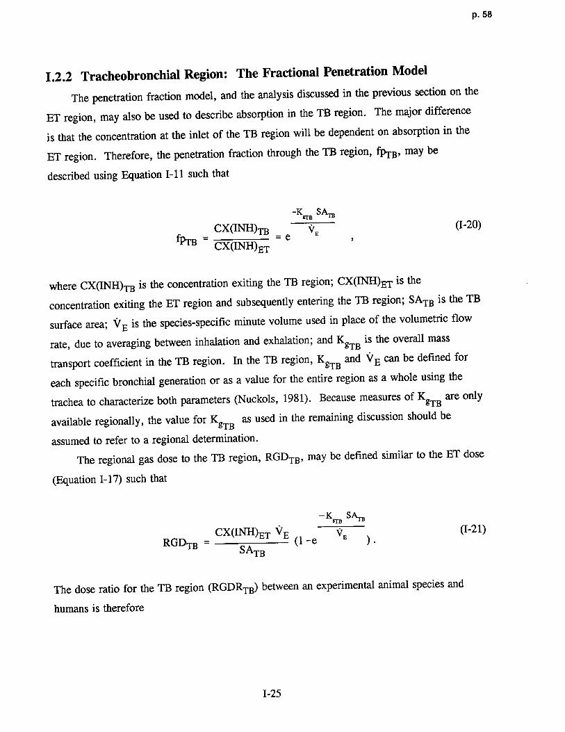
p. 58
1 .2.2 Tracheobronchial Region : The Fractional Penetration Model
The penetration fraction model, and the analysis discussed in the previous section on the
ET region, may also be used to describe absorption in the TB region. The major difference
is that the concentration at the inlet of the TB region will be dependent on absorption in the
ET region . Therefore, the penetration fraction through the TB region, fpTB, may be
described using Equation I-11 such that
-Krr
e SA.I.B
CX(INH)TB - e V E (1-20)
~TB CX(INH)ET
where CX(INH)TB is the concentration exiting the TB region ; CX(INH)ET is the
concentration exiting the ET region and subsequently entering the TB region ; SATB is the TB
surface area; VE is the species-specific minute volume used in place of the volumetric flow
rate, due to averaging between inhalation and exhalation ; and KgTB is the overall mass
transport coefficient in the TB region . In the TB region, KgTB and VE can be defined for
each specific bronchial generation or as a value for the entire region as a whole using the
trachea to characterize both parameters (Nuckols, 1981) . Because measures of KgTB are only
available regionally, the value for KgTB as used in the remaining discussion should be
assumed to refer to a regional determination .
The regional gas dose to the TB region, RGDTB, may be defined similar to the ET dose
(Equation 1-17) such that
-KVrB
SA,,
RGD CX(INH)ET VE (1 _e V E ) (I-21)
TB -SATB
The dose ratio for the TB region (RGDRTB) between an experimental animal species and
humans is therefore
1-25

p. 59
CX(INH)ET VE -Kera SATB
RGDR.I.B =(R
GD.I.B)A =SATB A (1 - e VE )A
(1-22)(RGDTB)H CX(INH)ET VE -KgrB SA'rB
SATB H (1 - e `'E )H
where A and H refer to laboratory an imals and humans, respectively . Assuming the same
inhaled concentration, the above dose ratio will be divided by Ci/Ci resulting in the
concentration ratio (CX(INH)ET/Ci) in the numerator and denominator for both laboratoryan imal and human . This concentration ratio is fpET . The resultant gas dose ratio to the TBregion is thereby
VE
-K
tr SAT,,
RGDRTB = (RGDTB)A - SATB A (fPET) A (1 - eV
E )A (1-23)(RGDTB)H VE (fpET) H -K
9TB SA,,
SATB H (1 - e vE )H
Thus, the results obtained from an evaluation of ET penetration are used to determine the
dose to the TB region .
Similar to the ET region, Equation 1-23 may be simplified when Kg is large (less than
5% error if KgTBSATB/ VE,I,B is greater than or equal to 3) such that Equation 1-23 becomes2
Note that Equation 1-24 may also be de rived from Equation 1-23 by determining the conditions whereby
SAra-KIT
B
(1-exp E )A~ 1 .
-K
SAT
BtrB V
(1 -exp E )H
These conditions will be a function of the default values for respirato ry tract surface area and minute volume as wellas the absolute value of the overall mass transpo rt coefficient .
1-26
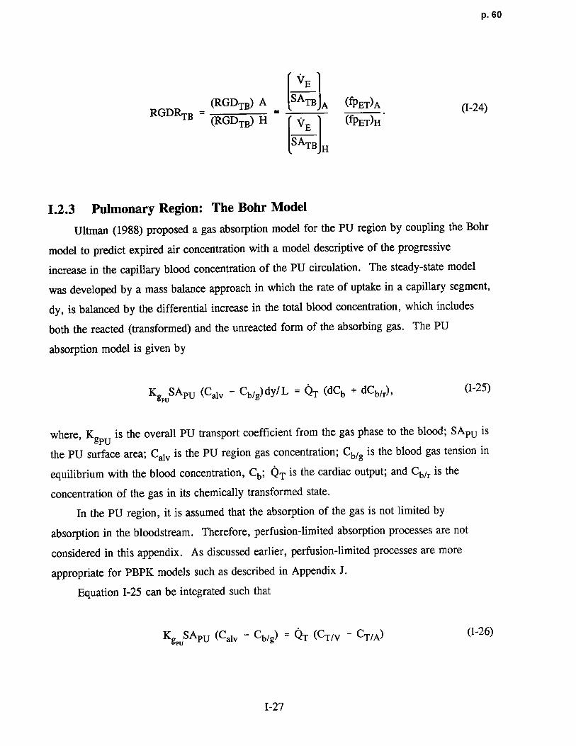
p. 60
VE
RGDRTB =(RGDTB) A a SATB A OPET)A (1-24)
(RGDTB) H VE (fPET)H
SATB H
1.2 .3 Pulmonary Region: The Bohr Mode l
Ultman (1988) proposed a gas absorption model for the PU region by coupling the Bohr
model to predict expired air concentration with a model descriptive of the progressive
increase in the capillary blood concentration of the PU circulation . The steady-state model
was developed by a mass balance approach in which the rate of uptake in a capillary segment,
dy, is balanced by the differential increase in the total blood concentration, which includes
both the reacted (transformed) and the unreacted form of the absorbing gas. The PU
absorption model is given b y
KgPUS`e'pU (Caiv - Cb/g) dy/ L = QT (dCb + dCb/r), (1-25)
where, KgPU is the overall PU transport coefficient from the gas phase to the blood; SAPU is
the PU surface area; Calv is the PU region gas concentration ; Cb/g is the blood gas tension in
equilibrium with the blood concentration, Cb; QT is the cardiac output ; and Cb/r is the
concentration of the gas in its chemically transformed state .
In the PU region, it is assumed that the absorption of the gas is not limited by
absorption in the bloodstream . Therefore, perfusion-limited absorption processes are not
considered in this appendix . As discussed earlier, perfusion-limited processes are more
appropriate for PBPK models such as described in Appendix J .
Equation 1-25 can be integrated such tha t
KgPU SAPU (Caiv - Cb/g) = QT (CT/V - CT/A) (1-26)
1-27
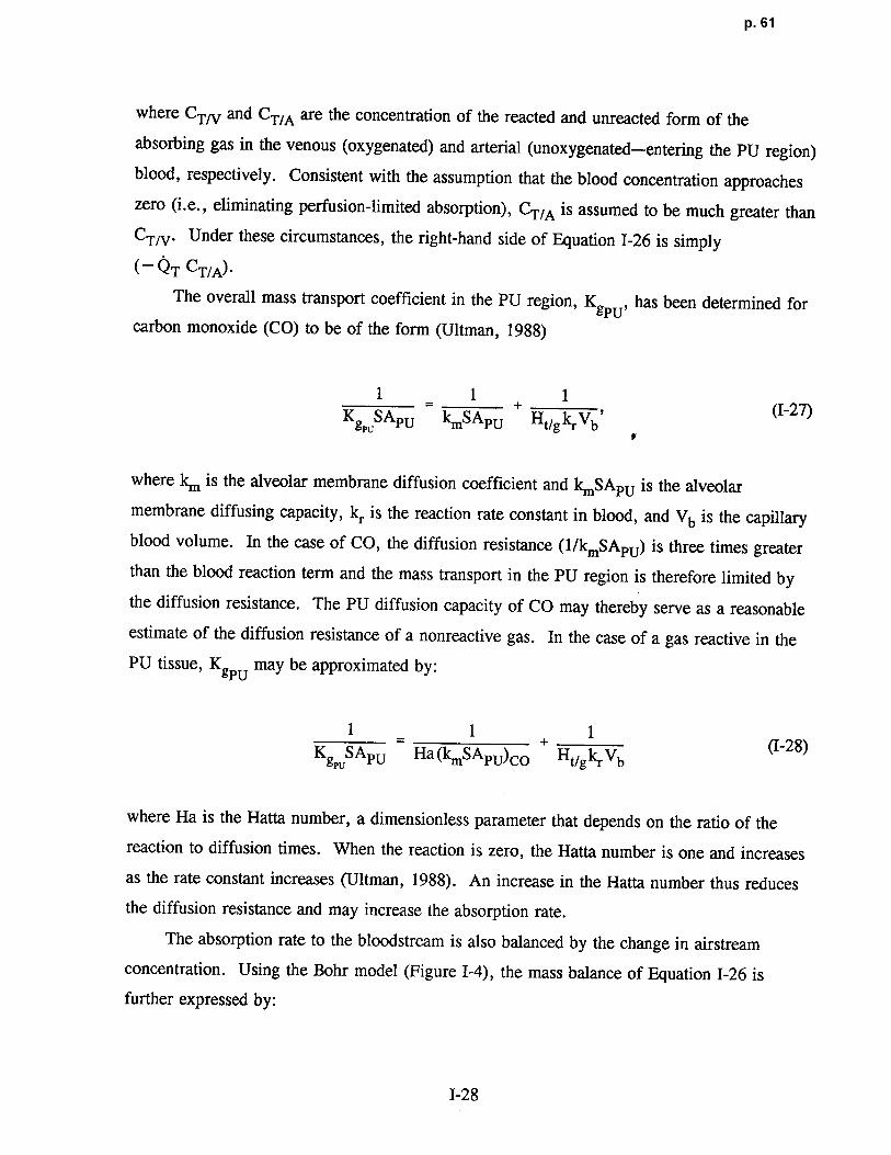
p. 61
where CTN and CT/A are the concentration of the reacted and unreacted form of th e
absorbing gas in the venous (oxygenated) and arterial (unoxygenated-entering the PU region)
blood, respectively . Consistent with the assumption that the blood concentration approaches
zero (i .e., eliminating perfusion-limited absorption), CT/A is assumed to be much greater than
CT/V . Under these circumstances, the right-hand side of Equation 1-26 is simpl y
(- QT CT/A)-
The overall mass transport coefficient in the PU region, KgpU, has been determined for
carbon monoxide (CO) to be of the form (Ultman, 1988 )
1 1 1+ ~ (1-27)
KgpoSAPu kmSAPU Ht/g kr Vb
where km is the alveolar membrane diffusion coefficient and kmSApU is the alveolar
membrane diffusing capacity, kt. is the reaction rate constant in blood, and Vb is the capillary
blood volume. In the case of CO, the diffusion resistance (1/kmSApU) is three times greater
than the blood reaction term and the mass transport in the PU region is therefore limited by
the diffusion resistance . The PU diffusion capacity of CO may thereby serve as a reasonable
estimate of the diffusion resistance of a nonreactive gas . In the case of a gas reactive in the
PU tissue, KgpU may be approximated by :
1 _ 1 1+ (1-28)KgpUSApU Ha (1mSAPU)co Ht/g kr Vb
where Ha is the Hatta number, a dimensionless parameter that depends on the ratio of the
reaction to diffusion times . When the reaction is zero, the Hatta number is one and increases
as the rate constant increases (Ultman, 1988). An increase in the Hatta number thus reduces
the diffusion resistance and may increase the absorption rate .
The absorption rate to the bloodstream is also balanced by the change in airstream
concentration . Using the Bohr model (Figure 1-4), the mass balance of Equation 1-26 is
further expressed by :
1-28

p. 62
CXTB
Q alv
C alv
CV QT CA
Figure 1-4. Bohr model of ventilation and uptake . The definitions for the parametersymbols are provided in Table I-1 .
Qa1v (CX(EXH)TB - Calv) - KgpUSAPU (Caiv - Cb/g) - - QTCT/AI (1-29)
where Q .1v is the alveolar ventilation rate.
The first two terms in Equation 1-29 are used to develop the ratio of the expired
concentration to inspired concentration, which will be used as a penetration fraction of the
PU region, fppU, defined as the ratio of Calv to CX(INH)TB such tha t
Calv _ Qalv _ (1-30)CX(INH)TB KgpUSApU (1 - Cb/g / Calv) + Qalv
However, for the case of diffusion-limited absorption, Cb/g is much less than Caiv such that
the denominator on the right hand side of the Equation 1-30 is simply (KgpUSApU + Qalv) .
I-29

p. 63
The regional gas dose (RGD) to the pulmonary region (PU) i s
RGDpU = (1 - fppU) QalvCX(INH)TB . (I-31)
PU
Combining Equation 1-30 and 1-31 results in the following relationship :
RGDpU = (1 -Qalv ) Qalv
CX(INH)TB , (I-32)
KgruSApU + Qa1v SAPU
where the regional gas dose ratio to the pulmonary region (RGDRpU) between laboratory
animal and humans is given by
(1 _ Qalv )A
RGDRpU = (RGDPU)A _ KgPOSAPU + Qalv (Qalv/SApU)A (CX(INH)TB),~ (1-33) .(RGDpU)H (1 _
Qalv ) (Qalv/SAPLJ)H (CX(INH)TB) H
HKgpUSAPU + Qalv
Dividing both numerator and denominator by the inspired air concentration converts the last
term to the product of the penetration fractions of the preceding regions such tha t
(1 -Qalv )A
(RGD
PU)A KgPVSAPU + Qalv (Qalv/SA)A (fPTB)A ( fPET)A~RGDRpU = = - (1-34)
(RGDpU)H (1 _ Qalv ) (Qa1v/SA)g (f~PU)H (fPET) H
HKgroSApU + Qalv
where the ratios (fpTB)A/(fpTB)H and (fPET)A/(fPET)H must be determined from the
penetration fraction model for the TB and ET regions, respectively . Equation 1-34 may be
further reduced to
1-30

p. 64
KgPUSApU )A ( Qa1v )ARGDRpU (RGDpU)A - KgPUSApU + Qal`' SAPU «TB)A (fPET)A
(1-35)- )
(RGDPU)H
(
KgpuSAPU Qa1v)H
(fpTB)H (fPET)H ~
KgpUSApU + Q~v)H (SApU
from which the limiting values for the dose ratio may be obtained . At large values of KgpU,
as would be the case for Category 1 gases, Equation 1-35 reduces to:
Qalv
(RGDpu)A=
( SApU)A (fPTB)A (fPET) ARGDRpU = - . (I-36)
~GDPU)H Qa1v )H (fpTB)H (fPET)H( SApU
1 .2.4 DEFAULT APPROACH FOR CATEGORY 1 GASE S
As mentioned earlier, more elaborate models such as those using a finite difference
solution to the convective-diffusive equation have been developed and applied to specific
gases for evaluation of local absorption rates (McJilton et al ., 1972 ; Miller et al., 1985) .
The method in this appendix presents a reasonable alternative based on fewer parameters and
one that is amenable to the types of uptake data routinely generated in some laboratories
(Morris and Smith, 1982 ; Stott and McKenna, 1984 ; Morris and Cavanagh, 1986, 1987 ;
Morris, 1990 ; Morris et al ., 1986, 1991 ; Dahl et al ., 1991b; Morris and Blanchard, 1992 ;
Bogdanffy et al ., 1991 ; Bogdanffy and Taylor, 1993; Kuykendall et al ., 1993). It is hoped
that this approach encourages development of these types of data for the various toxic air
pollutants that the inhalation reference concentration RfC methods are intended to address .
Because uptake data on which to base Kg values are not available for many toxic
chemicals, this section presents default approaches to those presented in the preceding
Section 1.2. The default approaches have been derived based on analyses of the limiting
conditions described in that section . It is assumed that the values for VE and the SA values
for the various respiratory tract regions will be constants within each species .
1-31
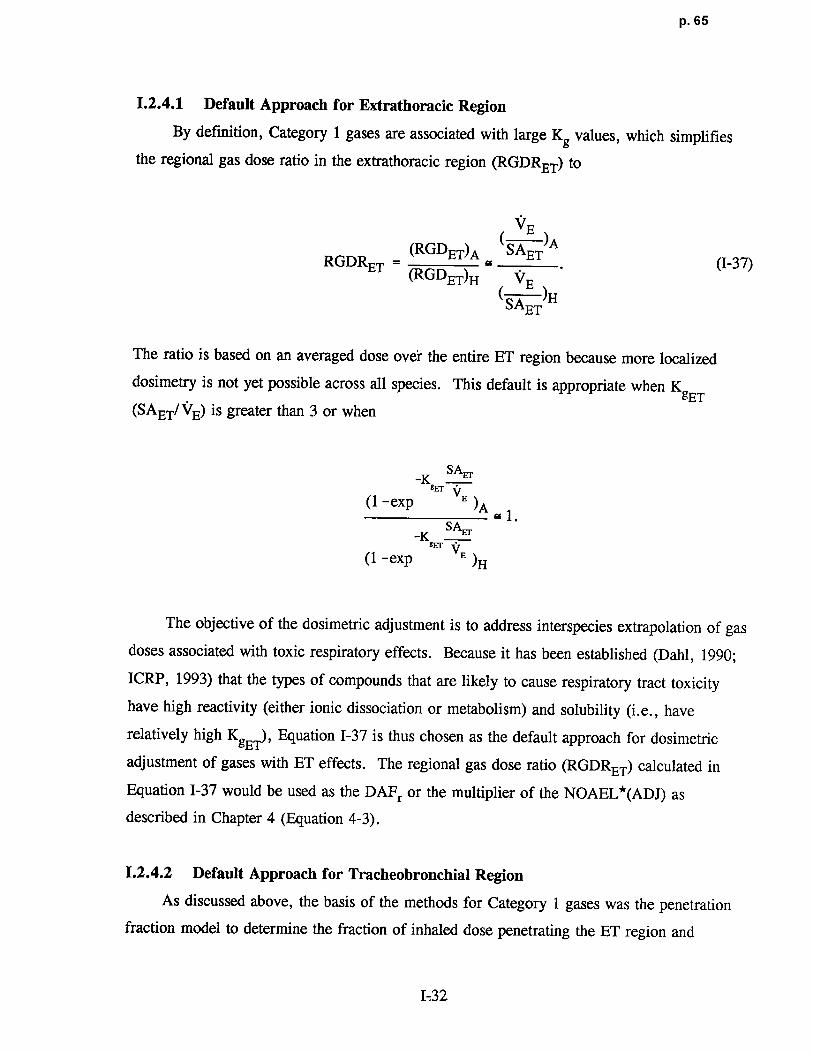
p. 65
1.2.4.1 Default Approach for Extrathoracic Region
By definition, Category 1 gases are associated with large Kg values, which simplifies
the regional gas dose ratio in the extrathoracic region (RGDRET) to
VE
)ARGDR = (RGDET)A SAETET (RGDET)H VE ' (I-37)
)HSAET
The ratio is based on an averaged dose over the entire ET region because more localized
dosimetry is not yet possible across all species . This default is appropriate when KgET
(SAET/ VE) is greater than 3 or when
-K SAE7
(1-exp BEr
VE )A~ 1 .
-K SAr
gFV(1 -exp E )H
The objective of the dosimetric adjustment is to address interspecies extrapolation of gas
doses associated with toxic respiratory effects . Because it has been established (Dahl, 1990 ;
ICRP, 1993) that the types of compounds that are likely to cause respiratory tract toxicity
have high reactivity (either ionic dissociation or metabolism) and solubility (i .e., have
relatively high KgE,I,), Equation 1-37 is thus chosen as the default approach for dosimetric
adjustment of gases with ET effects . The regional gas dose ratio (RGDRET) calculated in
Equation 1-37 would be used as the DAFr or the multiplier of the NOAEL*(ADJ) as
described in Chapter 4 (Equation 4-3) .
1 .2.4.2 Default Approach for Tracheobronchial Regio n
As discussed above, the basis of the methods for Category 1 gases was the penetration
fraction model to determine the fraction of inhaled dose penetrating the ET region and
1-32

p. 66
thereby available for uptake in the TB region . Thus, the regional gas dose ratio for th e
tracheobronchial region (RGDRTB) is calculated as
VE -Kg,rB SA,r B
_ (RGDTB)A _ [SABIA (fPET) A (1 - e VE )A (1-38)RGDRTB
(RGDTB)H VE (fPET) H -KeTB SATB
SATB H (1 - e VE )H
If the penetration fraction is unknown due to the lack of data on KgTB, it is reasonable to
assume that Kg is large, which is consistent with the definition of Category 1 gases, such that
the exponential term of Equation 1-38 reduces to zero . The same result may be achieved by
determining the conditions in which the third ratio of the right hand side of Equation 1-38
reduces to 1 . These conditions will be a function of the default values for respiratory tract
surface area and minute volume as well as the absolute value of the overall mass transport
coefficient . Using the definition of fpET results in the following dose rati o
VE -K SA Er
gEr
V(RGDTB)A SATB A (e E )A (1-39)RGDRTB
TB ( H VE -K SAErg
Er
y
[sB]H (e )H
which can be rearranged to
VE
SA~ 1Kesr)n
= (RGDTB)A _ S`~TB A e ERGDRTB
A (1-40)
(RGDTB)H VE _ SA 'J(Kser) H
SATB H VE H
1-33

p. 67
If (KgET) A can be assumed to be equal to (KgET) H, then Equation 1-40 can be further
simpli fied to
KBErE _
SA vEVERGDRTB =(RGD~)A = TB A e JA (1-41)
(RGDTB)H VV 1-QA
SAE
TH vE H
If KgET is further assumed to be one, Equation 1-41 reduces further such that only minute
volume and surface areas are needed to evaluate the dose ratio, such that :
VE _ S
AE
r
(RGDTB)A SATB A e E ARGDRTB = _ (1-42)
(RGDTB)H VE 1 _ SA!
rSATB H VE
H
If KgET is available for each species, Equation 1-39 would be the preferred default equation .
1 .2.4.3 Default Approach for Pulmonary Regio n
As discussed in Section 1 .2 .3, the regional gas dose ratio for the PU region (RGDRpU)is given by Equation 1-35 :
( KgPOSApU ) Qalv
)RGDRpU =
(RGDpU)A _ Kg
PUSApU + Qalv A ( SApUA (fP•rB)A (fPET)A (1-35)
~(RGDPU)H ( KgPO
S`e'pU
. ) (Qalv ) (fPTB) H (fPET)H
KgrvSApU + Qalv H SApU H
which at large KgpU values reduces to
I-34

p. 68
Qa1v
RGDRpU = (RGDPU)A - ( SAPUJA ( mB)A (fPET)A- , (1-43)
(RGDPU)H Qa1v (fPTB)H (fPET)H
SApUH
If the penetration fractions to each of the preceding regions are unknown due to lack of
data on KgET and KgTB, the approach to deriving a default equation for the PU region is
described below .
Using the definition of fpET and fpTB results in the following gas dose ratio for the PU
region :
S"-TB SAI,Qa1v -KgTB -KeEr
(RGDpU)A - (SApU)A (e VB )A (e VE )A (1-44)RGDRpU = RGD SAM sAE,.
( PU)H ( Qa1v ) -Kg.I .B V -K~ V
SApU H (e E )H (e E )H
which can be rearranged to
I Qaly-SAT. (KBTB)n -SAEr (KeFdn
RGDpU)A ISAPUJA le VE A VE ARGDRpU = (I-45)
(RGD PU)H Qalv SA TB (KgTB)H -SAEr (KBEC) H
ISAPUJH VE H VE H
If (KgET) A and (KgTB) A are assumed to be equal to (KgE~H and (KgTB)H, respectively,
then Equation 1-45 can be further simplified to
1-35
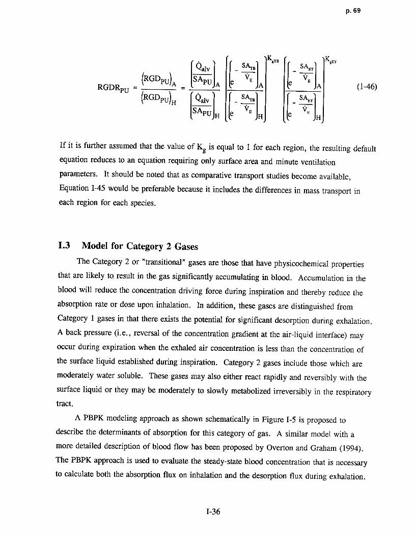
p. 69
Q SA.r KgTS SA KB~
alv _ B _ Er
(RGDPU)A S APU ee RGDRpU =A A A (1-46)
(RGDPU)H Qalv _ S'~B sA~.
[SApU]H fe VE H e VE H
If it is further assumed that the value of Kg is equal to 1 for each region, the resulting default
equation reduces to an equation requiring only surface area and minute ventilation
parameters . It should be noted that as comparative transport studies become available,
Equation 1-45 would be preferable because it includes the differences in mass transport in
each region for each species .
1.3 Model for Category 2 Gases
The Category 2 or "transitional" gases are those that have physicochemical properties
that are likely to result in the gas significantly accumulating in blood . Accumulation in the
blood will reduce the concentration driving force during inspiration and thereby reduce the
absorption rate or dose upon inhalation . In addition, these gases are distinguished from
Category 1 gases in that there exists the potential for significant desorption during exhalation .
A back pressure (i .e., reversal of the concentration gradient at the air-liquid interface) may
occur during expiration when the exhaled air concentration is less than the concentration of
the surface liquid established during inspiration . Category 2 gases include those which are
moderately water soluble. These gases may also either react rapidly and reversibly with the
surface liquid or they may be moderately to slowly metabolized irreversibly in the respiratory
tract .
A PBPK modeling approach as shown schematically in Figure 1-5 is proposed to
describe the determinants of absorption for this category of gas . A similar model with a
more detailed description of blood flow has been proposed by Overton and Graham (1994) .
The PBPK approach is used to evaluate the steady-state blood concentration that is necessary
to calculate both the absorption flux on inhalation and the desorption flux during exhalation.
1-36
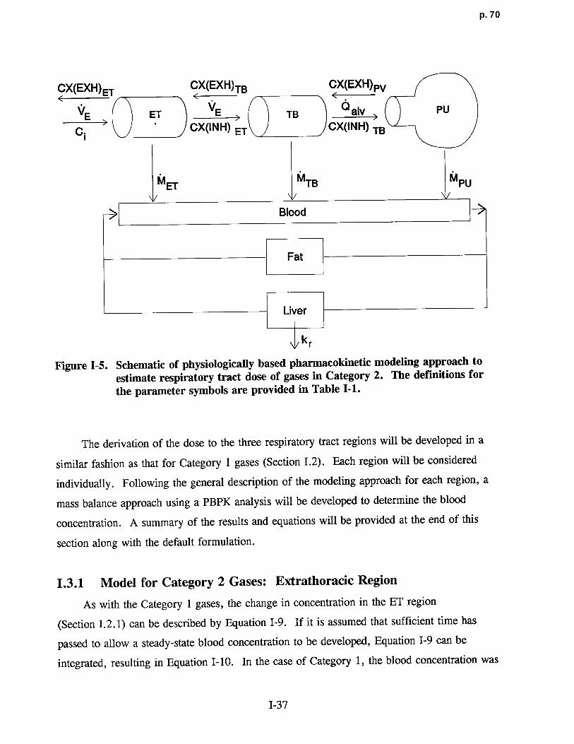
p. 70
CX(EXH)ET CX(EXH)TB CX(EXH)Pv
VE \ = ET VE ~ TB Q giy PU
C CX(INH) ET CX(INH) TB
MET MTB M PU
Blood
Fat
Liver
k r
Figure 1-5 . Schematic of physiologica lly based pharmacokinetic modeling approach to
estimate respiratory tract dose of gases in Category 2 . The definitions forthe parameter symbols are provided in Table I-1 .
The derivation of the dose to the three respiratory tract regions will be developed in a
similar fashion as that for Category 1 gases (Section 1 .2) . Each region will be considered
individually . Following the general description of the modeling approach for each region, a
mass balance approach using a PBPK analysis will be developed to determine the blood
concentration . A summary of the results and equations will be provided at the end of this
section along with the default formulation .
1.3 .1 Model for Category 2 Gases : Extrathoracic Region
As with the Category 1 gases, the change in concentration in the ET region
(Section I .2.1) can be described by Equation 1-9 . If it is assumed that sufficient time has
passed to allow a steady-state blood concentration to be developed, Equation 1-9 can be
integrated, resulting in Equation 1-10 . In the case of Category 1, the blood concentration wa s
I-37

p. 71
assumed to be much less than the airstream or interfacial concentrations . For Category 2,
however, the blood concentration must be retained . Thus, the fraction of gas that penetratesto the TB region is given by rearranging Equation I-10 such that:
-K SAE7
-K SA~
fpET - e
8
Er VE + Cb/g -e BEF vE (I-47)
Ci
As defined in Equation 1-16, the dose on inhalation to the ET region, RGD(INH)ET, may beobtained by substituting Equation 1-47 into Equation 1-16 and rearranging to obtai n
SAEr
RGD(INH)ET - 1 -SC-
(1 - e-Kg~ VE )C
1"E
(1-48)
SAET
The form of the overall mass transport coefficient in Equation 1-48 differs from that todescribe Category 1 gases because a term to describe the disposition of the gas in blood isrequired. Approaches to include this term are reviewed by Ultman (1988) . In the casewhere there is either no reaction or the reversible nature of the reaction can be handled byadjusting Ht/g to be in equilibrium with the dissociated form of the gas, the mass tr ansportcoefficient for Category 2 gases may be determined from :
1 =_ 1 + 1 + Sp ~
(1-49)KgEr kg Ht/gkl Hb/gQb
where Sp is the blood perfusion surface area, Hb is the blood :air part ition coefficient, and Qb
is the local blood flow rate . The mass transport coefficient for gases, which are moderately
to slowly metabolized in the tissue phase is given b y
1 1 + 1 + F~ (I-50)
Kgs,. kg Ht/gkl Hb/gkrVLG
1-38

p. 72
where F is the flux fraction reaching the blood, and VLG is the volume of lung tissue . The
flux fraction, F, is less than one if the absorbing gas reacts with constituents in the surface
liquid and tissue phases .
Equation 1-48 addresses the dose upon inhalation only . To evaluate the total dose,
including events occurring during exhalation, the potential for desorption and the desorption
flux must be evaluated. Desorption will reduce the total dose over a respiratory cycle ; the
dose associated with an observed effect is therefore less than that if only the dose on
inhalation was considered . In the following section, the desorption term is developed by first
considering the tissue depth in which desorption may influence tissue concentration and, by
analogy, tissue dose .
1.3.1.1 Theoretical Considerations for Modeling Desorptio n
Empirical data has indicated that desorption can be important to estimating the
respiratory tract dose (Gerde and Dahl, 1991 ; Dahl et al ., 1991b) . Unless the tissue
concentration is greater than the exhalation airstream concentration, there will be no
desorption during exhalation and, in fact, there is actually the potential for additional
absorption . To evaluate the potential desorption, it is assumed that the blood concentratio n
attains a relatively constant concentration independent of the respiratory flow cycle . Because
it is assumed that the potential desorption will not impact the blood concentration, desorption
will only impact the concentration profile in the tissue . The tissue concentration profile
during exhalation is a function of the duration of exhalation . If desorption occurs, the
surface-liquid/tissue concentration will decrease during exhalation, as will the concentration
gradient between the air (gas phase) and blood. An example of the change in the tissue
concentration profile that may occur during desorption is shown in Figure 1-6 .
In Figure 1-6, the change in tissue concentration is shown to penetrate the entire
surface-liquid/tissue phase as a result of the change in airstream concentration between
inhalation and exhalation, C(INH) and C(EXH), respectively . The extent to which the tissue
concentration profile changes is as yet unknown and must be evaluated to formulate the
desorption term . To estimate the depth in the tissue .that may be influenced by the change in
flow direction and hence airstream concentration, an analytic solution is employed to evaluate
the time course of the concentration profile in the tissue when the surface is expose d
1-39

p. 73
Airway Lumen
Gas Phase Surface-Liquid / Tissue Phase Blood
C(INH)@ t<0
C(EXH)@ t > 0 ----- --------- ---------------
------------- -
aS tEXHT ------ ---- ---- -- -- ----_ C b
OZ
F igure 1-6. Schematic of surface-liquid/tissue phase concentration during exhalation .
to a step change in concentration associated with the flow reversal . To avoid assumptions
about the tissue thickness, it is assumed that the tissue is infinitely thick .
In Figure 1-7, the initial conditions prior to imposing the step ch ange is shown in which
the tissue concen tration is Co throughout . At time zero (t=0), the step change in the
airstream concen tration is imposed and the change in tissue concen tration with distance and
time is illustrated . Given the conditions described above and further assuming no reaction in
the surface liquid-tissue layer, the solution is given in the form
~C CS-
C = erf z , (1-51)S O) 2 Dt
where CS is the imposed concentration ; CZ is the concentration in the surface liquid/tissue,
which is a function of time (t) and distance into the layer (z) ; CO is the initial concentration ;
1-40
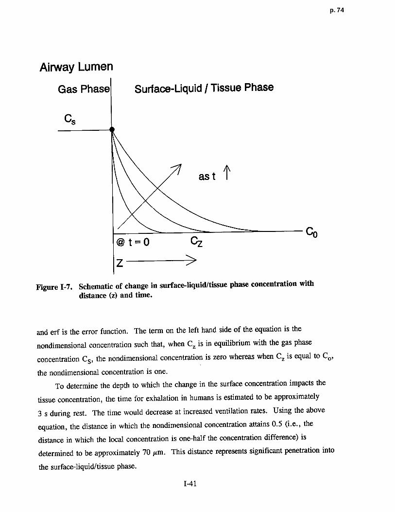
p. 74
Airway Lume n
Gas Phase Surface-Liquid I Tissue Phase
Cs
as t ~
@ t = 0 Cz Co
Z
Figure 1-7. Schematic of change in surface- liquid/tissue phase concentration with
distance (z) and time.
and erf is the error function . The term on the left hand side of the equation is the
nondimensional concentration such that, when CZ is in equilibrium with the gas phase
concentration CS, the nondimensional concentration is zero whereas when CZ is equal to Co,
the nondimensional concentration is one .
To determine the depth to which the change in the surface concentration impacts the
tissue concentration, the time for exhalation in humans is estimated to be approximatel y
3 s during rest . The time would decrease at increased ventilation rates . Using the above
equation, the distance in which the nondimensional concentration attains 0.5 (i .e., the
distance in which the local concentration is one-half the concentration difference) is
determined to be approximately 70 µm . This distance represents significant penetration into
the surface-liquid/tissue phase .
1-41

p. 75
1.3.1.2 Formulation of the Desorption Ter m
The above estimate indicates that an imposed step change in air (gas phase)
concentration as occurs du ring exhalation results in the tissue concentration at 70 µm attaining
50% of the equilibrium value within 3 s . Because this distance is of the order of the distante
between the air-surface liquid/tissue interface and blood (Miller et al ., 1985), it will be
assumed in the derivation of the desorption term that the entire depth of the surface liquid-
tissue phase between its interface with the gas phase and the blood may be impacted by
desorption . Thus, a conservative assumption would be to assume that the gradient of an
absorbing, nonreactive gas achieves a linear profile quickly du ring both inhalation and
exhalation and that the gas phase transport resistance does not affect desorption . Therefore,
the desorbed mass due to the flow reversal may be obtained by evaluating the change in mass
necessary to effectively reduce the tissue gradient from the inhalation gradient to the
exhalation gradient as indicated in Figure 1-8 .
Airway LumenGas Phase Surface-Liquid i Tissue Phase Blood
C(INH)
ContinuedC(EXH) Absorption
CIDAZ
C(EXH) - - - -- --- -- -- -"~'~`- ---° Desorption
Figure 1-8. Schematic of change in mass during breathing cycle .
1-42
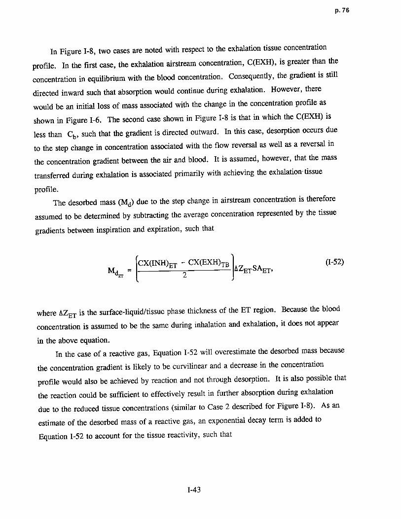
p. 76
In Figure 1-8, two cases are noted with respect to the exhalation tissue concentration
profile . In the first case, the exhalation airstream concentration, C(EXH), is greater than the
concentration in equilibrium with the blood concentration. Consequently, the gradient is still
directed inward such that absorption would continue during exhalation . However, there
would be an initial loss of mass associated with the change in the concentration profile as
shown in Figure 1-6 . The second case shown in Figure 1-8 is that in which the C(EXH) is
less than Cb, such that the gradient is directed outward . In this case, desorption occurs due
to the step change in concentration associated with the flow reversal as well as a reversal in
the concentration gradient between the air and blood . It is assumed, however, that the mass
transferred during exhalation is associated primarily with achieving the exhalation- tissue
profile .
The desorbed mass (Md) due to the step change in airstream concentration is therefore
assumed to be determined by subtracting the average concentration represented by the tissue
gradients between inspiration and expiration, such tha t
CX(INH)ET - CX(EXH)TB eZ SA (1-52)M~ = 2 ET ET ,
where AZET is the surface-liquid/tissue phase thickness of the ET region . Because the blood
concentration is assumed to be the same during inhalation and exhalation, it does not appear
in the above equation .
In the case of a reactive gas, Equation 1-52 will overestimate the desorbed mass because
the concentration gradient is likely to be curvilinear and a decrease in the concentration
profile would also be achieved by reaction and not through desorption . It is also possible that
the reaction could be sufficient to effectively result in further absorption during exhalation
due to the reduced tissue concentrations (similar to Case 2 described for Figure 1-8) . As an
estimate of the desorbed mass of a reactive gas, an exponential decay term is added to
Equation 1-52 to account for the tissue reactivity, such tha t
I-43
p. 77
MdEr _ CX(INH)ET - CX(EXH)TB -k (1-53)2 JAZETSAET e I
where tEXH is the time of exhalation .
The regional desorbed dose (mass/cm2 -time) during exhalation is therefore Md divided
by the product of the surface area and the exhalation time, such tha t
MRGD(EXH)ET = `~' , (1-54)
SAET tEXH
The total dose in the ET region, accounting for both absorption during inhalation and
desorption during exhalation, is therefore :
SA~.
C1VE Cb~ -K`~ v _ Md (I-55)RGD(TOTAL)ET = 1- g (1 - e E ETSAET Ci ) SAET tEXH •
1 .3.2 Model for Category 2 Gases : Tracheobronchial RegionThe model developed for the analysis of total dose to the ET region for gases in
Category 2 is directly applicable to the determination of the total dose to the TB region, such
that
RGD(TOTAL) = CX(INH)ET VE Cb/g __KBTB v e _ Me
TB SATB CX(INH)ET (1 e ) SA t 'TB EXH
(I-56)where the desorbed mass is similarly defined as above . Thus, for gases that do not reactirreversibly, Md is given by :
M _ CX(INH)TB - CX(EXH)pU(1-57)dre 2 A Z'TB SATB ,
1-44

p. 78
and for those gases that do react irreversibly Md is is given by
M=
CX(INH) TB CX(EXH)PU]AIFBSATB e
kr(6H) (1-58)
~B 2
where A7TB is surface-liquid/tissue phase thickness of the TB region.
Substituting for CX(INH)ET using Equation 1-47 and the definition of fpET
Equation 1-56 becomes
KgEr
SA Er - KgTB SA ra M
RGD(TOTAL)TB -C . VE e VE 1- C g (1 - e VE )- dTB (I-59)SATB 1 SATB EXH
1 .3.3 Model for Category 2 Gases : Pulmonary Region
The dose to the PU region for the Category 2 gases may be derived on the basis of
equations provided previously (Section 1 .2 .3) . From Equation 1-30 the ratio of the expired
concentration to the inspired concentration of this region (i .e., the penetration fraction of the
PU region) is defined as
CX(EXH)pU Qa1 v
CX(INH)TB Cb/ ' (I-60)g +KgpUSApU 1 - CX(EXH)pU Qalv
where CX(EXH)pu is the concentration exiting the PU region and therefore includes the
desorption term .
In the previous section describing PU dose (Section 1.2.3), Kgpu is defined only for a
reactive gas (Equation 1-28) . However, for gases that are nonreactive or reversibly reactive,
a more appropriate form would be (Ultman, 1988)
I-45

p. 79
1 __ 1+
Sp(1-61)
Kgpu Ht/gk1SApU Hb /gQb .
The PU dose as defined for Category 1 gases was based on the assumption that Cb /gwas less than Catv . This assumption is not applicable to the transitional gases of Category 2
because of the potential for elevated blood concentrations . Consequently, the total dose to
the PU region for these gases is defined as
RGD(TOTAL)pU = 1Qalv Qalv
CX(INH)SA TBCb/g PU
[KgPUSApU 1 CX(EXH)pU +0aiv] (1-62)
Equation 1-62, although the most general form of the PU dose, can also be formulated
more simply by assuming
Calv = CX(EXH)pU = Cb/g (1-63)
because Category 2 gases are moderately water soluble and likely to reach equilibrium
between alveolar air concentration and the blood . Under these conditions, the PU dose is
simply the difference between the inhaled concentration, CX(INH)TB, and the exhaled
concentration, CX(EXH)pU, such that
CX(INH)TB - CX(EXH)pURGD (TOTAL)pU = Qalv~ (I-64)
SApU
which by substitution for CX(INH)TB and CX(EXH)pU rearranges t o
1-46
p. 80
KErSAEr KgTBSATB
(1-65)RGD(TOTAL)PU = Ci
Qaiv 1-" Cblg) (e Vg ) (e VE )
\
SApu C
Equation 1-65 represents the most generalized equation resulting from the simplifying
assumption that the PU dose is proportional to the difference between the inhaled and exhaled
concentrations .
1 .3.4 Modeling the Blood Compartment for Category 2 Gase s
As defined, Category 2 gases will accumulate in the blood . Thus, an explicit derivation
to determine concentration of the gas in the blood is required to solve for the dose into each
region. In particular, the term that must be evaluated is (1- Cb /g/Cl), which appears in each
of the equations necessary to solve the regional dose . This term includes the blood
concentration because Cb /g is the concentration in the gas phase which would be in
equilibrium with the blood (i .e., Cb/g = Cb/Hb /g) .
The blood concentration is derived by a mass balance approach . It is assumed that the
systemic blood compartment is well mixed so that the change in concentration is due to the
input mass delivered through the respiratory tract, loss due to metabolism in the lung tissue,
redistribution of the gas in the systemic compartments (including the fat compartment) during
intermittent exposures, and loss due to systemic metabolism (modeled in the liver
compartment), such that
Vb daCb E(RGD(TOT)RTSA(TOT)RT) - Cart(CLsys + CLfa) - VLGELG (1-66)
where Vb and VLG are the volumes of the blood and lung compartments, respectively, Cb is
the average blood concentration; E(RGD(TOT)RT SA(TOT)RT) is the summed product of the
dose and surface area of each region in the respiratory tract ; Cart is the arterial blood
concentration ; CLsys and CLfat are the clearance from the systemic (i .e., assumed to be
dominated by the liver compartment) and the fat compartments, respectively ; and BLG is the
elimination rate in the lung compartment due to metabolism . The total mass transport rate to
I-47

p. 8 1
the respiratory tract (mass/time) is given in the above equation as the summed product of the
dose and surface area of each region in the respiratory tract . However, the total dose to the
respiratory tract may also be obtained by the difference in inhalation and exhalation
concentrations, such tha t
E (RGD(TOT)RTSA(TOT)RT) = VE (Ci - CX(EXH)ET) . (1-67)
The term that implicitly includes the blood concentration and is necessary to solve
regional dose is obtained from Equation 1-67 . Ignoring further absorption or desorption that
may occur during expiration, CX(EXH)ET may be approximated by CX(EXH)pU, which is
equivalent to Cg,„ the alveolar concentration, which is in equilibrium with the blood
(Equation 1-63) . Thus
VE (Ci - CX(EXH)ET) = VECi (1 - Cb/g). (1-68)Ci
To determine the respiratory tract dose during the exposure, it will be assumed that the
system is in quasi-steady state such that the change in the average blood concentration
(dCb/dt) is zero (Equation 1-66) . Under these conditions, the mass delivery rate to the
respiratory tract surface (defined in Equation 1-67) is equal to the loss due to clearance from
the liver and fat as well as metabolism in the respiratory tract tissue . Combinin g
Equations 1-66 through 1-68 under steady state conditions results i n
VE (Ci - Caiv) = Cart(CLsys + CLfat) + VLGELG• (1-69)
This relationship, however, can be further reduced for Category 2 gases .
In the case of gases that are relatively insoluble in water (Category 3, Appendix J), the
fat compartment plays an important role in the distribution of the gas . The fat compartment
may absorb mass at the start of and/or during an intermittent exposure and therefor e
1-48

p. 82
represents an additional loss from the arterial blood concentration . At the end of the
exposure, leaching from the fat compartment may be an additional input to the blood .
Because the initial dose of gases with respiratory toxicity accounts for the dose that may be
leached subsequently from the fat, no additional dose following the end of exposure needs to
be accounted for . Furthermore, the contribution of the fat compartment is reduced for
Category 2 gases because the gas will not partition significantly to the fat because of its lower
fat to blood partition coefficient. In addition, the concentrations in the systemic
compartments are in equilibrium with the blood during steady state . Thus, the uptake by the
fat will be assumed zero, consistent with the definition Category 2 gases because of their
partition coefficient . The assumption of a steady state is conservative because it will
underestimate the dose to the respiratory tract compartments that are the objective of the
derivation in this appendix . The assumptions of steady state and of equilibrium between
tissue and blood compartments results in the elimination of CLfat from Equation 1-69 .
Rearranging Equation 1-69 to solve for systemic elimination results in
CL(Ci - Caiv) VLGELG (1-70)
sys = VE - ,Cart Cart
where CLfat is zero as described above. However, the ratio of the exhaled concentration,
Caiv , to Cart is approximated by Hb/g . Equation 1-70 may therefore be rewritten a s
VLGELG (1-71)Sys =V( - )- ,
E HEFF Hb/g Cart
where HEFF is the steady state blood to inhaled gas concentration ratio observed in an
experimental situation (Andersen, 1981), which is referred to here as an effective partition
coefficient .
It is now necessary to more specifically incorporate the loss terms for systemic
clearance and respiratory tract metabolism . It will be assumed that systemic clearance is
I-49
p. 83
predominately due to metabolism in the liver and is given by (Andersen, 1981 ; Pang and
Rowland, 1977)
CLSys = CLLIV = QTET, (I-72)
where CLLIV is the clearance from the liver compartment ; Qr is the cardiac output ; and
ET is the liver extraction efficiency . The elimination rate from the lung compa rtment, ELG 9is defined according to Michaelis-Menton kinetics :
CLGVMAX
ELG = (KM + CLG) = kLGCLG, (1-73)
where VMAX is the maximum velocity of saturable (Michaelis-Menton) metabolism path ;
where CLG is the lung tissue concentration ; KM is the Michaelis constan t; and kLG is the
elimination rate from the lung compartment .
Combining Equations 1-71 to 1-73 provides the loss terms in relation to HEFF :
QTEI' = VE(H 1 1 ) _V LGkLG Cart (1-74)EFF
Hb/g a rt
Assuming the respiratory tract tissue concentration, CLG, is in equilibrium with the blood, the
ratio CLG/Cart is equivalent to the tissue :blood partition coefficient, Ht/b. Solving for HEFF
yields
HEFFVE
-VE (1-75)
QTET + VLGkLGHt/b + Hb/g
Combining Equation 1-68 with the definition of Hb/g and HEFF results in
1-50

p. 84
H HCb/ b/g EFFVECi (1- Clg) = VE(Ci - Calv) = VECi ( H ~-76
)
b/g
Upon substitution of 1-75 into 1-76, the term necessary to solve the dose ratio in
Equations 1-55, 1-59, and 1-65 is obtained :
(1 _ Cb/g ) _ QTETHb/g + VLGkLGHt/bHb/g (I-77)
Ci QTFTHb/g + VLGkLGHt/bHb/g + VE '
where Ht/g is equal to the product of Ht/b and Hb/g . Equation 1-77 may be simplified by
considering the range of partition coefficients, extraction efficiency and the respiratory tract
tissue concentration .
At large values of Ht/g (and consequently Hb/g since Hb/t x Ht/g = Hb/g), the term on
the right hand side of Equation 1-77 approximates one . Therefore, Cb/g << Ci which is the
definition of Category 1 gases (i .e ., those gases that are highly soluble and/or rapidly
irreversibly reactive) for which the approach presented in Section 1 .2 .4 applies . This case is
consistent with a greater extraction efficiency of the respiratory tract relative to the systemic
clearance as well as absorption proximal to the PU region . Conversely, at low values of
Ht/a, absorption proximal to the PU region is negligible and the relative efficiency ofb
systemic clearance is greater than that of the respiratory tract extraction (as well as uptake) .
The approach for category 3 gases presented in Appendix J applies in this case .
The remaining gases are those which are moderately water soluble (intermediate value
of Ht/g) and are therefore the Category 2 gases . For Category 2 gases, Equation 1-77 reduces
to
(1 - Cb/g) = QT F`rHb/a (1 +
VLGkLGHt/b (1-78)
Ci VE b QTET
since VE/ QTHb/g » F-r + (VLGkLG/ (~r) Ht/b-
1-51

p. 85
Equation 1-78 can be further reduced since Or approximates VE . The magnitude of the
blood concentration is determined by the relative significance of the metabolism which occurs
in the respirato ry tract versus systemic elimination (as shown in the rati o
VLGkLGHt/b/ (~rFT) • If systemic elimination is much larger, Equation 1-78 reduces t o
(1 - CC/
g) = ETHb/g (1-79)
i
At the maximum, it will be assumed that the respirato ry tract elimination would be equal to
that of the systemic elimination under which circumstance s
(1 - CC/g) = 2~Hb/g . (1-80)i
It will be further assumed that the systemic elimination term is defined for maximum
elimination, i .e. assuming liver saturation kinetics, such that ET is defined by EMAX, the
maximum extraction efficiency. The maximum extraction efficiency is approximatel y
0 .25 QT . due to the flow limitation to the liver (Andersen, 1981) . Thus, Category 2 gases can
be defined based on systemic elimination and the relative significance of respiratory tract
metabolism to systemic elimination .
1 .3.5 Default Approach for Category 2 Gases
The default approach is developed by ignoring the desorption associated with exhalation .
This assumption may be valid in as much as the mass in the tissue that is desorbed during
exhalation is replaced on inhalation . Whether, in general, this assumption results in an
overestimate or underestimate of the dose is not clear because ignoring the desorbed mass
may not significantly impact the concentration driving force ( i .e ., the concentration of the gas
at the surface-liquid/tissue interface and the concentration in the blood may be proportionately
affected) .
In comparing cyclic absorption-desorption and unidirectional absorption, the
concentration at the interface between the air and surface liquid is likely to be lower in the
1-52
p. 86
case of desorption and the driving force would therefore be lower than in the case o f
unidirectional absorption if the blood concentration were equal in both cases . The net effect
would suggest that ignoring desorption would overestimate the absorbed mass or dose .
However, by overestimating the absorbed mass in the case of unidirectional absorption, the
blood concentration will be elevated over the absorption-desorption case . The elevated blood
concentration will also reduce the concentration driving force . Therefore, although ignoring
desorption will increase the surface liquid concentrations, the blood concentration will
similarly be overestimated, so that the concentration driving force may not be dissimilar than
with desorption described.
The dose to each region, ignoring desorption, is therefore obtained by combining
Equation 1-79 or 1-80 (depending on the significance of respiratory tract metabolism) with
each of the individual dosimetry calculations in Equations 1-55, 1-59, and 1-65 for the ET,
TB, and PU regions, respectively .
1.3 .5.1 Default Approach for Extrathoracic Region
From Equation 1-54, the regional gas dose ratio (ignoring desorption) for the ET region
(RGDRET) is given by
VE Cb/g -K SAE
(RGDET)A - (C1SAETA (1 Ci )A (1 - e gE VE ) A
RGDRET = . (1-81)
(RGDET)H (C VE (1 - Cb/g) -K SAs`. )1 SAET H Cl H(1 - e gEr VE ) H
However, KgET for Category 2 gases is by definition less than 1 . Assuming KgET is equal to
or less than 0.5, a power series expansion of the exponential term results in the following
relationship :
I-53

p. 87
(C; E ) (1 -Cb/g) (-Kg~ SAET)
(RGDET)A 'SAET A Ci A VE ARGDRET =
(RGDET)V C SA (I 82)
H (C1SAE ) (1 C/g (-Kg~ VET
ETg 1 H E H
Assuming the same inspired concentration, simplifies the RGDRET to
(RGD ) K (1-CC/g)
RGDRET = ET A - g~TA ' A(1-83)
(RGDET)H KgErH (1-Cb/g)
C1 H
If the overall mass transport coefficients (KgET) are assumed equal as in the case of Category
1 gases, the regional gas dose ratio is reduced to the ratio of (1 - Cb/g/Ci) .
Two cases were developed for the derivation of the blood term as expressed in
Equations 1-79 and 1-80. The first case in which systemic elimination is assumed to be much
greater than respiratory tract metabolism such tha t
(RGDET)A
Kg~A
(0.25 QTHb/g)ARGDRET = (1-84)
(RGDET) H KgEr
H (0 .25 QTHb/g)H~
and the second case in which respiratory tract metabolism is assumed to be of equal
significance with systemic elimination such tha t
(RGDET) Kg (0.5 QTHb/ )RGDRET =
A = ETA g A (1-85)(RGDET)H KgErH (0.5 QTHb/g)H
I-54
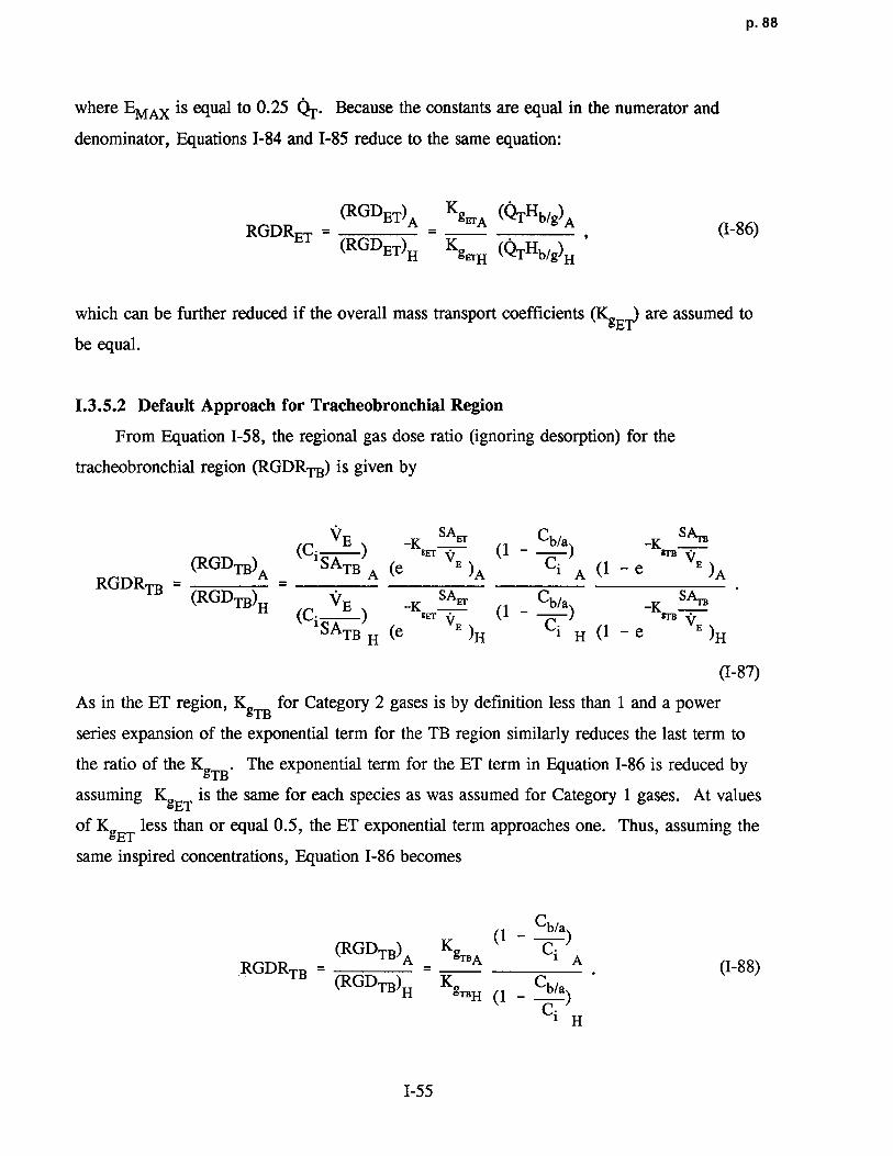
p. 88
where EMAX is equal to 0 .25 Q . Because the constants are equal in the numerator and
denominator, Equations 1-84 and 1-85 reduce to the same equation :
(RGDET)A _ Kg~.A (QTHb/g)ARGDRET (1-86)= (RGDET)H KgErH (QTgb/g) H
which can be further reduced if the overall mass transport coefficients (KgE,i,) are assumed to
be equal .
1.3.5.2 Default Approach for Tracheobronchial Regio n
From Equation I-58, the regional gas dose ratio (ignoring desorption) for the
tracheobronchial region (RGDRTB) is given by
(Cl VE ) -Kg~ SA El (1 _ Cb/a -KSAM
(RGDTB)A - SATBA (e E )A
Ci A(1 - e E )A
RGDRTB = •(RGDTB)H VE -K gEr
SAET(1 -
Cb/a -K S``1'ra(Ci SATB)H (e vE )H Ci H(1 - e VE )H
(1-87)
As in the ET region, KgTB for Category 2 gases is by definition less than 1 and a power
series expansion of the exponential term for the TB region similarly reduces the last term to
the ratio of the KgTB. The exponential term for the ET term in Equation 1-86 is reduced by
assuming KgET is the same for each species as was assumed for Category 1 gases . At values
of KgET less than or equal 0.5, the ET exponential term approaches one . Thus, assuming the
same inspired concentrations, Equation 1-86 becomes
(1Cb/a
RGDRTB = (RGDTB)A
=Kg.r
BA Ci A (1-88)(RGDTB)g KgTBH (1 _ Cb/a )
C1 H
I-55

p. 89
As above, Equation 1-88 is further reduced by substituting Equation 1-79 for the case in
which systemic elimination predominates :
RGDRTB _ KgTBA (0.25 QTHb/a)A (1-89)TB (RGDTB)H KgTBH (0
.25 QTHb/a)H
By substituting Equation 1-80 for the case in which respiratory tract metabolism and systemic
elimination are of equal significance, Equation 1-88 becomes :
(RGDTB)A _ KgTBA (0.5 QTHb/a)A (1-90)RGDR =TB _ I-(RGDTB)H KgTBH (0
.5 QTHb/a)H
where EMAX is equal to 0 .25 QT. Because the constants are equal in the numerator and
denominator, Equations 1-89 and 1-90 reduce to the same equation :
RGDRTB _ KgTa,~ (QTHb/a)A (1-91)TB (RGDTB)H KgTBH (QTHb/a)
H
which can be further reduced if the overall mass transport coefficients (KgTB) are assumed to
be equal .
1 .3.5.3 Default Approach for Pulmonary Region
From Equation 1-64, the regional gas dose ratio (ignoring desorption) for the PU region
(RGDRpu) is given by
Qalv _K SA Er SAT,
(Ci ) ger VgrB V (1 - )
(RGDpU)A SApU
A(e E)A (e E)A Ci ARGDRpU
(RGDPU)H (C Qalv ) -K SA~ Cb/a)g~ V-K SAT,
V B ( I -
1 SApU H (e E)g (e E)g C' H
(1-92)
1-56
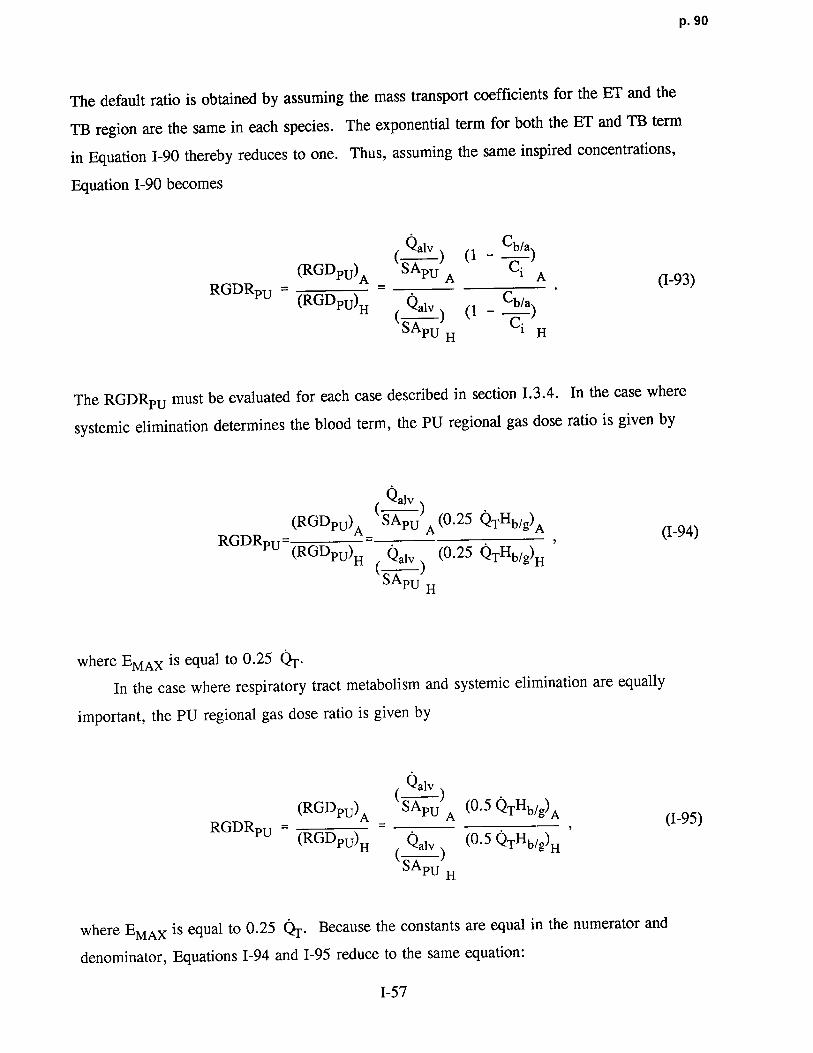
P. 90
The default ratio is obtained by assuming the mass transport coefficients for the ET and th e
TB region are the same in each species . The exponential term for both the ET and TB term
in Equation 1-90 thereby reduces to one . Thus, assuming the same inspired concentrations,
Equation 1-90 becomes
Qa1v (1 Cb/a
RGDRpU =(RGDpU)A - SApU A C .
A (1-93)
(RGDPU)H Q 1v (1 - Cb/a
SApUH Ci H
The RGDRpU must be evaluated for each case described in section 1 .3 .4. In the case where
systemic elimination determines the blood term, the PU regional gas dose ratio is given by
Qa1v
(RGDpU)A - SApU A (0 .25 QTHb/g) ARGDRpU = - , (1-94)
(RGDpU)H ( Qa1v (0.25 QTHb/g) H
SApU H
where EMAX is equal to 0 .25 QT .
In the case where respiratory tract metabolism and systemic elimination are equally
important, the PU regional gas dose ratio is given by
Qalv
(RGDpU)A SApUA (0 .5 QTHb/g) A (I-95)RGDRpU(RGDPU)H Qalv (0.5 QTHb/g)H
SApUH
where EMAX is equal to 0 .25 QT. Because the constants are equal in the numerator and
denominator, Equations 1-94 and 1-95 reduce to the same equation :
1-57
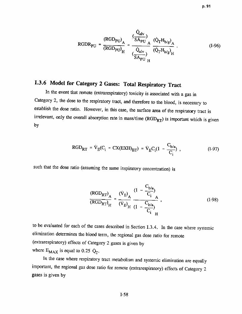
P. 91
Qalv
RGDR = ~GDPU)A - SAPU A (QTHb/g)APU - (RGD ) (1-96)
PU H ( Qa1v ) (QTHb/g)H
SApUH
1.3.6 Model for Category 2 Gases : Total Respiratory Tract
In the event that remote (extrarespiratory) toxicity is associated with a gas in
Category 2, the dose to the respiratory tract, and therefore to the blood, is necessary to
establish the dose ratio . However, in this case, the surface area of the respiratory tract is
irrelevant, only the overall absorption rate in mass/time (RGDRT) is important which is given
by
RGDRT = VE(Ci - CX(EXH)ET) = VECi(1 - CC/a) , (1-97)i
such that the dose ratio (assuming the same inspirato ry concentration) is
_ Cb/a)(RGDRT)A (VE)A (1 Ci A
(RGD (1-98)RT)H (VE)H (1 - Cb/a )
C1 H
to be evaluated for each of the cases described in Section 1 .3.4 . In the case where systemic
elimination determines the blood term, the regional gas dose ratio for remote
(extrarespiratory) effects of Category 2 gases is given b y
where EMAX is equal to 0 .25 QT. .
In the case where respiratory tract metabolism and systemic elimination are equally
important, the regional gas dose ratio for remote (extrarespiratory) effects of Category 2
gases is given by
1-58
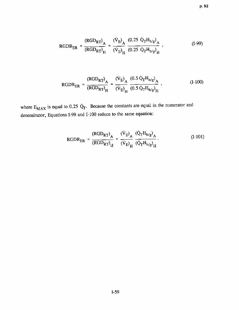
p. 92
(RGDRT)A (VE)A (0 .25 QTHb/g)A (1-99)
RGDRER = (RGD)RT g (VE)H (0.25 QTHb/g) H
(RGDRT)A - (VE)A (0.5 QTHb/g)A (1-100)
RGDRER = (RGDRT)H (VE)H (0.5 QTHb/g)H
where EM AX is equal to 0.25 QT. Because the constants are equal in the numerator and
denominator, Equations 1-99 and 1-100 reduce to the same equation :
(RGDRT) A _ (VF)A (QTHb/g)A (1-101)
RGDRER =(RGDRT)H (Vg)H (QTHb/g)H
1-59

p. 93
APPENDIX J . DERIVATION OF AN APPROACH TODETERMINE HUMAN EQUIVALENT
CONCENTRATIONS FOR EXTRARESPIRATORYEFFECTS OF CATEGORY 3 GAS EXPOSURE S
BASED ON A PHYSIOLOGICALLYBASED PHARMACOKINETIC MODEL
USING SELECTED PARAMETER VALUES
This appendix describes in detail the derivation of the procedure used in Chapter 4 to
estimate no-observed-adverse-effect level human equivalent concentrations (NOAEL L xEC]s)
for extrarespiratory effects of gases (or vapors) in Category 3 . The derivation is
mathematical in nature in that the equations of state that describe the disposition of inhaled
compounds in a generalized physiologically based pharmacokinetic (PBPK) model are
manipulated so as to obtain a conservative estimate (with respect to the model assumptions) of
NOAEL [xECI s as a function of the average animal exposure concentrations (NOAEL [ADJ]) .
A PBPK model is used because of the success of this type of model . For example, PBPK
models that describe the body as five compartments (gas exchange and the fat, poorly
perfused, richly perfused, and liver/metabolizing tissue groups) have been applied
successfully to estimating the internal concentrations of chemicals (e .g ., styrene, methanol,
and ethylene dichloride) for the purpose of risk assessment . Although PBPK modeling is the
choice procedure in risk assessment for dose extrapolation, this approach is not possible
without the values of physiological and biochemical parameters used in the modeling process,
nor without a thorough understanding of the agent's mechanism of action . These data
generally are not available for most compounds .
The proposed method is based on a PBPK model in which all of any number of
compartments are in parallel and in which for any compartment there can be any number of
paths of removal by linear and saturable processes . Selected relevant parameter values are
replaced by qualitative assumptions about species similarity and the response of internal
concentrations to exposure scenarios . In order to obtain a NOAEL[xEC]9 the assumption is
made that the effective dose for dose-response purposes is the arterial blood concentration of
J-1
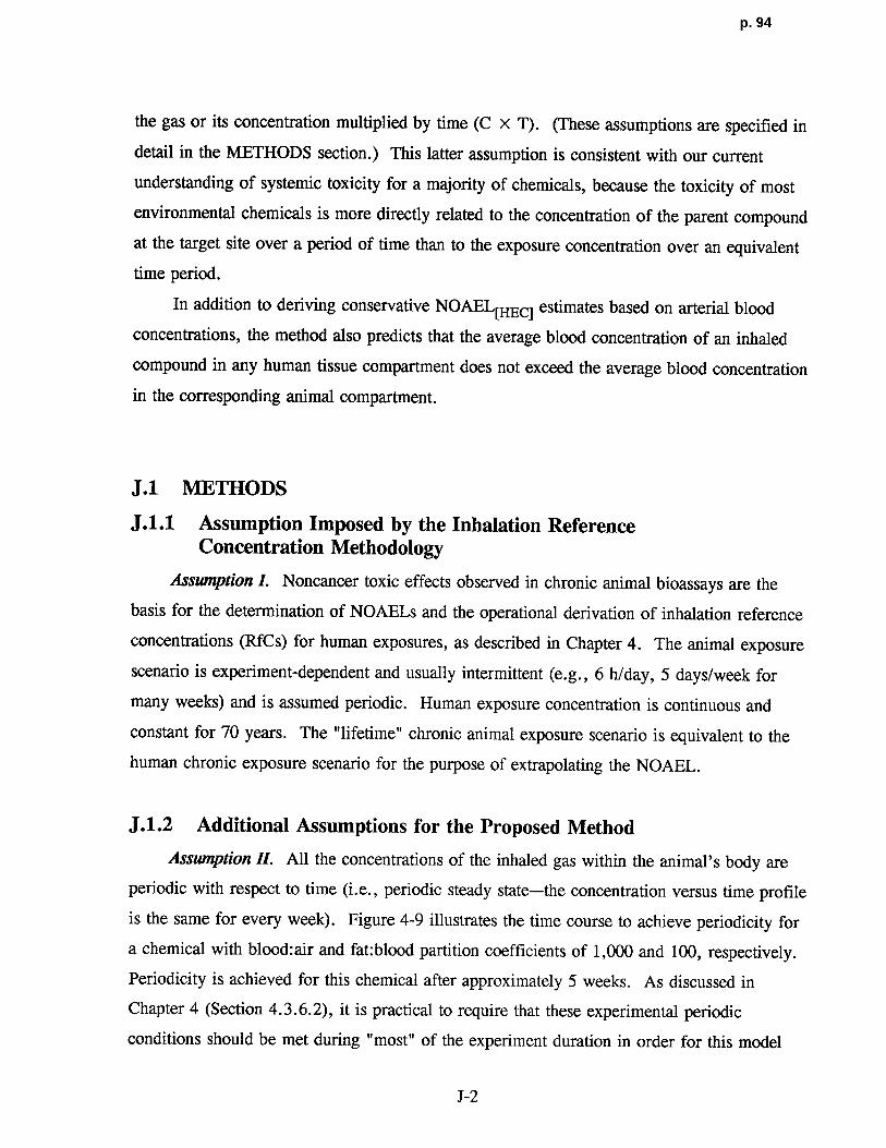
p. 94
the gas or its concentration multiplied by time (C X T) . (These assumptions are specified in
detail in the METHODS section .) This latter assumption is consistent with our current
understanding of systemic toxicity for a majority of chemicals, because the toxicity of most
environmental chemicals is more directly related to the concentration of the parent compound
at the target site over a period of time than to the exposure concentration over an equivalent
time period .
In addition to deriving conservative NOAEL [xEC] estimates based on arterial blood
concentrations, the method also predicts that the average blood concentration of an inhaled
compound in any human tissue compartment does not exceed the average blood concentration
in the corresponding animal compartment .
J.1 METHODS
J.1 .1 Assumption Imposed by the Inhalation ReferenceConcentration Methodology
Assumprion I. Noncancer toxic effects observed in chronic animal bioassays are the
basis for the determination of NOAELs and the operational derivation of inhalation reference
concentrations (RfCs) for human exposures, as described in Chapter 4 . The animal exposure
scenario is experiment-dependent and usually intermittent (e .g ., 6 h/day, 5 days/week for
many weeks) and is assumed periodic . Human exposure concentration is continuous and
constant for 70 years . The "lifetime" chronic animal exposure scenario is equivalent to the
human chronic exposure scenario for the purpose of extrapolating the NOAEL .
J.1.2 Additional Assumptions for the Proposed Method
Assumption II. All the concentrations of the inhaled gas within the animal's body are
periodic with respect to time (i .e., periodic steady state-the concentration versus time profile
is the same for every week). Figure 4-9 illustrates the time course to achieve periodicity for
a chemical with blood :air and fat:blood partition coefficients of 1,000 and 100, respectively .
Periodicity is achieved for this chemical after approximately 5 weeks . As discussed in
Chapter 4 (Section 4 .3.6.2), it is practical to require that these experimental periodic
conditions should be met during "most" of the experiment duration in order for this model
J-2

p. 95
application to result in an accurate estimate for use in the dose-response analysis . For
example, if the condition is met for nine-tenths of the time (e .g ., periodic du ring the last
90 weeks of a 100-week experiment), then estimates of average concentrations will be in
error by less than 10% . Thus, the requirement for application of this model is tha t
periodicity is achieved for 90% of the exposure period. If this is likely not to have occurred,
additional uncertainty in the extrapolation is imparted and should be addressed by an
uncertainty factor (Section 4 .3.6.2). During most of the time humans are exposed, given
Assumption I of continuous exposure, their internal concentrations are const ant and in
dynamic equilibrium with their exposure concentration .
Assumption III. A PBPK model describes the uptake and disposition of inhaled
compounds in animals and humans. The model is diagramed in Figure J-1, and the equations
of state are given by Equations J-1 through J-6. Table J-1 defines the variables and constants
in the equations .
dMp/dt = Qa1v x(CE - Cp + QT x(CV - CA) - rp(CA) (J-1)
dMj/dt = Qj x(CA - Cj) - rj(Cj); j 1,2,3, . . .n (J-2)
rp(CA) = VKFpi X CA +[VMAXpi x CA/(KMpi + CA)] (J-3a)i i
rj(Cj) = VKFji X Cj + [VMAXji X Cj/(KMji + G)] ; j = 1 to n (J-3b)i i
QT X CV = Qj X Cj (J-4)J
QT = ~ Qj (J-5)J
CA = Hb/g X Cp (J-6)
The equations describe a model with the following properties : (1) in the respiratory
tract compartment, the air, tissue and capillary blood concentrations are in equilib rium with
J-3
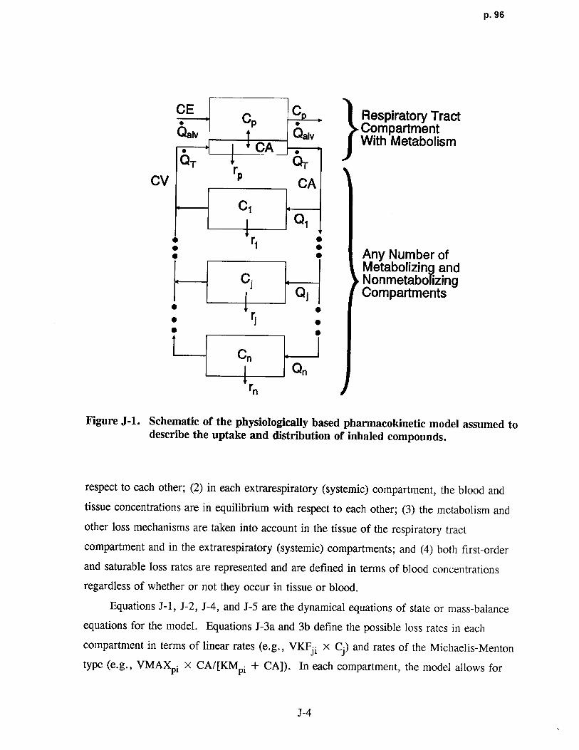
p. 96
C .., C C Respiratory Tract.' Compa rtmentQa1' Qa 1" With MetabolismCA ,[QT r
pC~
CV CA
C1Q,
: r1 : Any Number ofMetabolizing and
Cj NonmetabolizingQ j Compartments
• •• ri
CnQn
rn
Figure J-1 . Schematic of the physiologically based pharmacokinetic model assumed todescribe the uptake and distribution of inhaled compounds .
respect to each other ; (2) in each extrarespiratory (systemic) compartment, the blood and
tissue concentrations are in equilibrium with respect to each other ; (3) the metabolism and
other loss mechanisms are taken into account in the tissue of the respiratory tract
compartment and in the extrarespiratory (systemic) compartments ; and (4) both first-order
and saturable loss rates are represented and are defined in terms of blood concentrations
regardless of whether or not they occur in tissue or blood .
Equations J-1, J-2, J-4, and J-5 are the dynamical equations of state or mass-balance
equations for the model . Equations J-3a and 3b define the possible loss rates in each
compartment in terms of linear rates (e.g., VKFji x Cj) and rates of the Michaelis-Menton
type (e.g., VMAXpi x CA/[KMpi + CA]) . In each compartment, the model allows fo r
J-4
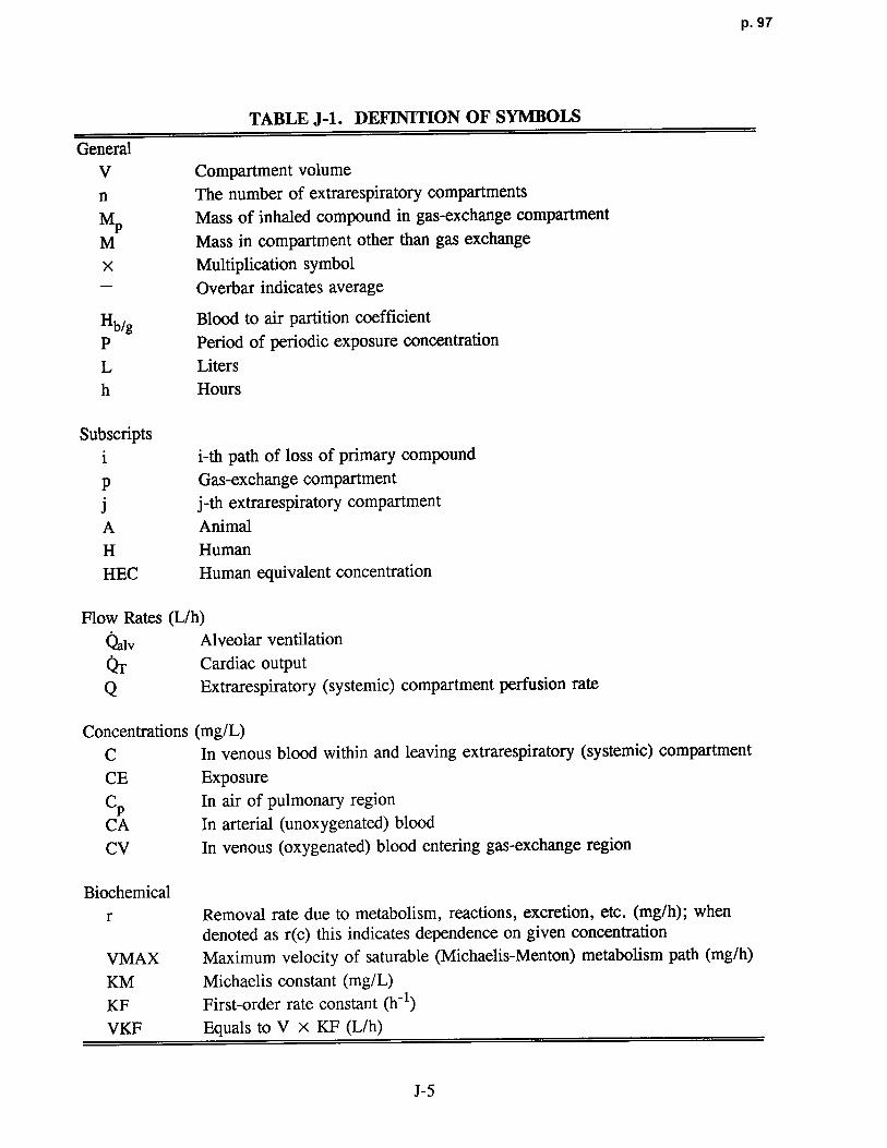
p. 97
TABLE J-1 . DEFINITION OF SYMBOLS
GeneralV Compartment volume
n The number of extrarespiratory compartment s
MPMass of inhaled compound in gas-exchange compartment
M Mass in compartment other than gas exchang e
x Multiplication symbol
- Overbar indicates average
Hb/g Blood to air partition coefficien t
P Period of periodic exposure concentration
L Liters
h Hours
Subscriptsi i-th path of loss of primary compoundp Gas-exchange compartment
j j-th extrarespiratory compartment
A Animal
H HumanHEC Human equivalent concentration
Flow Rates (L/h)
Qalv Alveolar ventilation
Or Cardiac outputQ Extrarespiratory (systemic) compartment perfusion rate
Concentrations (mg/L)C In venous blood within and leaving extrarespiratory (systemic) compartment
CE ExposureCp In air of pulmonary region
CA In arterial (unoxygenated) bloo d
CV In venous (oxygenated) blood entering gas-exchange region
Biochemicalr Removal rate due to metabolism, reactions, excretion, etc . (mg/h); when
denoted as r(c) this indicates dependence on given concentration
VMAX Maximum velocity of saturable (Michaelis-Menton) metabolism path (mg/h)
KM Michaelis constant (mg/L)
KF First-order rate constant (0)
VKF Equals to V X KF (L/h)
J-5
p. 98
more than one path of elimination or metabolism or for no losses (i .e., set both of a
compartment's kinetic parameters, VKF and VMAX, to zero) . Equation J-6 gives the
assumed relationship between the arterial blood concentration and the concentration in the air
of the pulmonary region .
According to Assumption I, the exposure concentration is periodic for laboratory
animals and constant for humans; in both cases, concentration of exposure (CE) can be
written as
CE = f(t) x CE, (J-7)
where :
ICE = the average exposure concentration, and
f = a periodic function of time (t) such tha t
f(t + P) = f(t) (J-8a)
t+P
f f(t) x dt = 1; (J-8b)
t
and P is the period of the periodic exposure concentration .
Assumption IV. Because the toxicologically effective dose to a given target tissue
depends on the animal species and chemical compound, its specification is typically not
available so that definition of a surrogate dose must be somewhat arbitrary . However, the
toxic effects of some compounds are expected to be directly related to the inhaled parent
compound in the blood . Furthermore, the use of the average blood concentration is an
internal dose "closer" to the target than a dose based on exposure concentration . Basing the
effective dose extrapolation on another surrogate (e .g., metabolite) would require knowledge
of the mechanisms of action and additional information about human and animal physiological
parameters . Thus, for animal to human exposure extrapolation, the human equivalent
J-6

P. 99
exposure concentration (CE[xECI) is defined in terms of the average arterial bloo d
concentration of the inhaled parent compound by requiring that the human equilibrium
concentration of arterial blood be less than or equal to the time-averaged arterial blood
concentration of the animal; that is, CAH <L7A. Note that the time average concentrations
are the area under the curve over a period divided by the length (time) of a period (e .g.,
average concentration over 1 week) . The equality condition defines the upper limit on an
acceptable human arterial blood concentration; thus, for mathematical simplicity this
assumption is formulated as :
CAH = Z,TAA. (J-9)
Because of this requirement, CAH is a function of UEA, because UAA depends on C'EA .
Assumption V. Similarity of species is assumed in that KM and the ratios Q/ (~,` „
VKF/ Qalv, and VMAX/ Qa1v are defined as species independent for each removal process (see
Table J-1 for definitions) . The invariance of the first ratio is based on the assumption that
the percent of blood flow to any compartment is independent of species and that cardiac
output (OT = sum of all Qj) scales, with respect to body weight, in the same way as the
ventilation rate (Qalv) ; (i .e., the ratio of QT to Qalv is species-independent) . The metabolic
constants VMAX and VKF are assumed to scale in the same way as Qai, . Justification for
this assumption about rates is based on the observation that for many species, rates scale in
the same way with respect to body weight (e .g ., in proportion to basal metabolism, body
surface area, or body weight to some power) (Dedrick, 1973 ; WeiB, 1977 ; Dedrick and
Bischoff, 1980; Boxenbaum, 1982 ; Rowland, 1985 ; Travis and White, 1988 ; Travis et al.,
1990; Federal Register, 1992b) . The invariance of the ratios VKF/ Qalv and VMAX/ Qa1v
follows .
Most of the above assumptions are well supported by data on comparative anatomy and
physiology, as detailed in the cited and other allometry references (Federal Register, 1992b) .
Collectively, they embody the concept of a basically similar mammalian physiological and
anatomical plan that varies primarily in scale from one species to another . The most
J-7

p. 100
problematic issue is the scaling of rates of individual metabolic transformation reactions as
BW3/4. Not only are there few data on such scaling, but some individual metabolic enzyme
systems have been shown to vary across species (Federal Register, 1992b) . However, several
points should be made. First, there are data that support the proposition of BW314 in specific
cases (Federal Register, 1992b) . For example, these same scaling assumptions have been
used in successful PBPK modeling across species (Ramsey and Andersen, 1984 ; Andersenet al., 1987a; Ward et al ., 1988; Allen and Fisher, 1993 ; Fisher and Allen, 1993) . Second,
overall metabolic rate (oxygen consumption, resting metabolic rate) clearly scales as BW3/4
Indeed, this is the issue around which physiological allometry was developed . Scaling an
individual metabolic step in this way corresponds to keeping it in proportion to general
metabolism, which seems the best default (Federal Register, 1992b) . Third, daily intake of
natural toxins (the usual targets of toxicant-metabolizing enzymes) depend on intake of air,
water, and food which all scale as BW3/4 . That is, scaling detoxification processes in
proportion to their anticipated load also predicts BW3/4 . Variation around scaling as BW3/4
does not invalidate the general scaling argument, nor does it provide evidence for any
different scaling factor . Rather, the variation simply illustrates that any single conception of
interspecies scaling can accommodate only the general trends, not the diversity of particular
instances (Federal Register, 1992b) . Clearly, as proposed in Section 3 .2 .2, when data or
more sophisticated models are available for interspecies extrapolation, they should be used in
preference to the default method presented herein .
Subject to the Assumptions, Equations J-1 to J-9 must be manipulated to determine
CEHEC as a function of the average animal exposure concentration, JCTA . Because the
concentrations and masses of a parent compound within a compartment are assumed to be
periodic, the integral of the left-hand side (LHS) of Equations J-1 and J-2 over a time length
of the period is zero ; for exampl e
t+P
f(dM/dt') X dt' = M(t + P) - M(t) = 0. (J-10)
t
J-8

p. 101
Also note that for equilibrium or steady state, as in the human case, the LHS of each of thes e
equations (J-1 and J-2) is zero by definition . Performing the period average of both sides of
Equations J-1 to J-6, the follow g are obtained :
0 = Qalv (CE - p) + QT X (CV - ~) - rp (J-11)
0= Qj x(CA - ~j) - rj ; j= 1, 2 1 3, . . . n (J-12)
(J-13a)rP = VKFpi X ZrA + ~ [VMAXPi X ~A7(I i + CA]]i
T)Tr~ = VKFji x +[VMAXji x j ji + j,; j 1 to n (J-13b)
i i
QT X UV = Qj X Ii (J-14)
QT = Qj (J-15)~
Z,rA = Hb/g X P (J-16)
The steady-state equations for umans are obtained from Equations J-1 and J-2 by setting the
LHS of these equations to zero (the equilibrium or steady-state condition) . The complete set
of equations of state for humans can be obtained from Equations J-11 through J-16 b y
redefining the average concen tions or terms as equilibrium values (i .e., remove the
overbars) .
The above equations are implified by combining Equations J-11 and J-16 to give
(QalvIHb/g + Q ) X ~A = (Qalv X UE) + (QT X UV) - ip , (J-17)
and Equation J-12 is expressed as
Qj xUA=Qj xCj+ii ;j =1ton . (J-18)
J-9

p. 102
Both sides of Equations J-17 and J-18 are divided by a1v 4) and Qj , respectively, to giv e
u xUA = Z,'E + w x UV - rp/Qalv , and (J-19a)
CA =-cj + rj /Qj; j= 1 to n, (J-19b)
where :
w = QT/Qalv, and
u = (Hb/g + QT/Qalv)
According to Assumption V, w is species independent . The parameter u is species-dependent
(via Hb/g) and will be identified as such with subsc ripts A and H for laboratory animal and
human , respectively . For simplicity and unless otherwise noted, averaged concentrations
(indicated by overbar) will be those of an imals and nonaveraged (no overbar) concentrations
will be those of hum ans .
Applied to humans, Equations J-19a and J-19b are written as
UH X CA = CE + w x CV - rpH(CA)/Qa1vH ~and
CA = Cj + rjH(Cj)/QjH ; j= 1 to n.
For laboratory animals, Equations J-19a and J-19b are w ritten as
UA x CA CR + w x CV - rpA/Qa1vA~ and (J-20c)
C N_C i + rjA/QjA; i 1 to n. (J-20d)
The loss terms in Equations J-3, rp(CA) and the ri
. (Cj)'s, are concave functions with th e
property that their second derivatives with respect to CA and CP respectively, are less than or
J-10
p. 103
and also,
-~ -~UA - UH = Hb/gA - Hb/gH .
Thus, Equation J-24 can be written a s
(Hb/gA-1 - Hb/gH-1) X UA > Z~ -CE +w x (T-V -CV), or (J-26a)
CE > CE + w x (CV - CV) + (Hb/gH-1 - Hb/gA-1) X UA. (J-26b)
Comparing Equations J-22b and J-23b, and using J-25b one sees that the bloo d
concen tration of the inhaled compound in any human compartment is less than or equal to theaverage blood concentration in the corresponding an imal compartment; that is
C. < T7 .. (J-27)
Because of Assumption V, (QjA/ QrA = QjH/ Q-rH), it follows from Equation J-14app lied to both humans and animals, and from Equation J-27, that
CV < Cp. (J-28)
Thus, the term w x(Z4V - CV) > 0 can be dropped from Equation J-26b without
affecting the inequality .
CE > CE + (Hb/gH-1 Hb/gA-1) X UA (J-29)
Note that CE is the constant inhaled hum an concentration that would give rise to a humanconstant blood level that is no greater than CA . If we choose the actual human exposure
concentration to be less than or equal to this CE, as defined by CA =CA, then the actualhuman arterial blood concen tration will be less than or equal to CA.
J-12
p. 104
equal to zero. As a consequence, the average of each of these functions is less th an or equal
to the function evaluated at the average concentration . Suppressing the subscripts, this
property is expressed as
r < r(c). (J-21)
Considering Equations J-21, J-20c, and J-20d, the following is noted :
uA X UA >_ CE + w X CV - rpA(C7~)/Qa1vA , and (J-22a)
~A <~+ rjA(~)/QjA ; J= 1 to n . (J-22b)
Using Equation J-9, Assumption IV (in the presentation notation, CA = CT ) ,
Equations J-20a and J-20b for human are written in terms of the an imal a rterial blood
concentration by replacing CA with CA as follows:
UH XCA = CE + w X CV - rpH(C`A)/QalvH (J-23a)
L7 = Cj + rjH(Cj)/Qjg; j= 1 to n . (J-23b)
Subtract the LHS and the right hand side (RHS) of Equation J-23a from the LHS and
RHS of Equation J-22a, respectively, to obtain
(uA - UH) X CW > CE - CE + (w X UV - w X CV) - (rpATA)/QalvA - rpH (CA)/QalvH)•
(J-24)
Because of Assumption V, for any concentration value, C,
rpA(C)/QalvA = rpH(C)/Qa1vH, and
rjA(C)/QjA = rjH(C)/QjH ;
J-11
p. 105
The following two cases are now considered with respect to the partition coefficient .
Case I: Hb/gA >_ Hb/gH
The second term on the RHS of Equation J-29 is greater than or equal to zero ; thus, the
term can be dropped from the RHS without affecting the inequality. Obviously, with respect
to model assumptions, a conservative human exposure concentration is UE . Therefore, in
terms of the variables in Chapter 4, an estimated conservative NOAEL*[HECI is given by
NOAEL*(HECI NOAEL*[ADJI, (J-30)
where:
NOAEL~[ADJI = the observed NOAEL or analogous effect level concentrationobtained with an alternate approach as described in Appendix A,adjusted for exposure duration (Equation 4-2) .
Case II: Hb/gA < Hb/gH
The second term on the RHS of Equation J-29 is negative in this instance . The inhaled
concentration must be greater than or equal to the exhaled concentration ; this requires that
UE > p or ~A < Hb/gA X~ . In Equation J-29, CT can be replaced by the larger
value, Hb/gA X CE, and still preserve the inequality, hence
CE >CE +(Hb/gH-i - Hb/gA-1) X Hb/gA XUE, or (J-31a)
CE > CE x (Hb/gA/Hb/$H). (J-31b)
In this case, an estimated conservative NOAEL*[gECI is given b y
J-13
p. 106
NOAEL* [HEC] = (Hb/gA/Hb/gH) X (Hb/gA/Hb/g) X NOAEL[ADJ] (J-32)
where:
NOAEL*IADJI = the observed NOAEL or analogous effect level concentrationobtained with an alternate approach as described in Appendix A,adjusted for exposure duration (Equation 4-2) .
J.2 AN EXAMPLE OF THE RELATIONSHIP BETWEEN THEPROPOSED AND OTHER METHODS
A perspective on the proposed method can be attained by examination of Figures J-2
and J-3, plots of NOAEL*[HEC] versus NOAEL*[A] for the rat and mouse, respectively .
These plots were created by choosing the equivalent exposure concentration that resulted in
the human arterial blood concentration being equal to the average arterial blood concentration
of the animal, using several methods, for the representative volatile organic compound
dicholoromethane (DCM) .
In Figures J-2 and J-3, the "previous" method refers to the method of using the ratio of
the ventilation rate divided by body weight in the laboratory animal to the ventilation rate
divided by body weight in the human ratio for calculating NOAEL*[HEC] estimates (Federal
Register, 1980), with the modification that alveolar ventilation rates are used (U .S.
Environmental Protection Agency, 1988a) . The NOAEL*lADJl of the laboratory animal
(Equation 4-2) is multiplied by the ratio to calculate the NOAEL*[HEC, estimate using this
method . "Optimal" method refers to the use of a specific PBPK model with an extensive set
of experimentally determined physiological parameters for the three species (Andersen et al .,
1987a) . The same model and human parameters were used for the "similar" method, but the
animal parameters were determined by scaling from the human values, as defined in
Assumption V . The "proposed" results are based on the methods proposed in this document
and derived in this appendix .
In keeping with the results of the derivation that is the subject of this appendix, the
"proposed" NOAEL*[HEC, estimates are less than the "similar" method estimates . With
J-14

p. 107
1,000DichloromethaneRat ' -:
:/
~. %--~
E '... ;
* =100
lJJ : / - -
o ---z
; ' ~~-- " optimal,- i _ ---- Similar
Proposed••-•-•-•• Previous
1010 100 1,000 10,000
NOAELA (mg/ms)
Figure J-2. Plot of NOAEL*[HECl versus NOAEL*[A] for the rat for four possiblemethods (proposed, previous, similar, and optimal) of determiningNOAELVMCI estimates as defined in the text. For any given observedNOAEL [A), the corresponding HEC estimate is found by going up to themethod(s) line and over to the y axis. The inhaled compound isdichloromethane . NOTE: NOAEL*lAl = animal NOAEL*1ADjl .
Source: Overton and Jarabek (1989a,b) .
respect to the relationship of the proposed predictions to the other methods of calculation, the
following observations are noted .
The "proposed" method lines are parallel to the "previous" lines and result in 3 .4 and
6.9 times smaller, or more conservative, NOAEL*[HEC] estimates than the "previous"
method for the rat and mouse, respectively . The "proposed" rat NOAEL*[HEC] estimates
also fall below (i .e., are more conservative than) those of the "optimal" method by a range of
1 .4 to 2 .4. Except at high exposure concentrations (above approximately 1,600 mg/m3),
where the estimates are smaller by about 1 .3, the "proposed" mouse NOAEL*[HEC] estimates
are up to 1 .5 times greater than the "optimal" NOAEL*[HEC] estimates . This supports
current evidence that the mouse is not "similar" to humans in some cases (Reitz et al ., 1988) .
However, for this species, the "proposed" method estimates more closely approximate the
J-15

p. 108
1,000Dichloromethane : ~ .Mouse
% / -
E 'CDE
100
/ .-; /.-
QO Optimal
,Z ' / ---- SimilarProposed
% /-- ------• Previous; /_-
A -1010 100 1,000 10,000
NOAELA (mg/m3)
Figure J-3 . Plot of NOAEL*WC] versus NOAEL*lA] for the mouse for four possiblemethods (proposed, previous, similar, and optimal) of determiningNOAEL*~C ] estimates as defined in the text . For any given observedNOAEL*lA~, the corresponding HEC estimate is found by going up to themethod(s) line and over to the y axis . The inhaled compound isdichloromethane . NOTE: NOAEL*lAj = animal NOAEL*[ADJ] •
Source: Overton and Jarabek (1989a,b) .
"optimal" method estimates than do the "previous" estimates and the "proposed" method is
conservative (estimates all fall below) the "similar" method . It also should be noted that the
"optimal", "similar", and "proposed" methods result in smaller NOAEL*[HEC] estimates for
the mouse relative to the rat for the same exposure concentration, whereas the previou s
methodology results in the opposite relationship of estimates between the two species .
J.2.1 Discussion
Considering the "optimal" method estimates to represent the best possible dose
extrapolation based on internal blood concentrations, then the "proposed" method is more
realistic than the "previous" method . Because the blood :air partition coefficients are more
J-16

p. 109
readily available than are complete physiological parameter data, the proposed metho d
represents a simple default approach when extensive PBPK modeling is not feasible .
J.2 .2 Research and Development
The approach presented in this appendix has resulted from modeling research focused on
determining the key parameters of gas uptake, distribution, and target tissue accumulation .
Future efforts will incorporate the anatomic and some aspects of the clearance data being
compiled for research to support the particle model described in Appendix G . Model
evaluation plans include comparing the efficiency of various dose surrogates and an approach
to address the apparent nonsimilarity of the mouse . Application of the model to address
mixtures of gases and of dose partitioning between gas and particles is also envisioned.
J-17