ownership structure and financial performance: … structure and financial performance: evidence...
TRANSCRIPT

DEPARTMENT OF ECONOMICS WORKING PAPER SERIES
Ownership Structure and Financial Performance:
Evidence from Panel Data of South Korea
Sanghoon Lee
Working Paper No: 2008-17
University of Utah
Department of Economics
1645 East Central Campus Dr., Rm. 308
Salt Lake City, UT 84112-9300
Tel: (801) 581-7481
Fax: (801) 585-5649
http://www.econ.utah.edu

Ownership Structure and Financial Performance:
Evidence from Panel Data of South Korea
Sanghoon Lee University of Utah, Department of Economics
Abstract
The study seeks to examine the effect of equity ownership structure on firm financial
performance in South Korea. I focus on the role of two main dimensions of the ownership
structure: Ownership concentration (i.e., the distribution of shares owned by majority
shareholders) and identity of owners (especially, foreign investors and institutional
investors). Using panel data for South Korea in 2000--2006, I find that firm performance
measured by the accounting rate of return on assets generally improves as ownership
concentration increases, but the effects of foreign ownership and institutional ownership are
insignificant. I also find that there exists a hump-shaped relationship between ownership
concentration and firm performance, in which firm performance peaks at intermediate levels
of ownership concentration. The study provides some empirical support for the hypothesis
that as ownership concentration increases, the positive monitoring effect of concentrated
ownership first dominates but later is outweighed by the negative effects, such as the
expropriation of minority shareholders. The empirical findings shed light on the role
ownership structure plays in corporate performance, and thus offer insights to policy makers
interested in improving corporate governance systems in an emerging economy such as
South Korea.
Keywords: Ownership Structure, Ownership Concentration, South Korea
JEL Classification: G32, G34

INTRODUCTION
This study seeks to examine the effects of equity ownership structure on firm
financial performance in South Korea and focuses on the role of two main dimensions of
the ownership structure, ownership concentration (i.e., the distribution of shares owned
by majority shareholders) and ownership identity (especially, foreign investors and
institutional investors). Ownership structure is an important internal mechanism of
corporate governance.
Corporate governance is an issue of growing importance, both theoretically and
practically. However, corporate governance had been largely ignored in the mainstream
economics literature. The traditional theory of the firm is based on a concept of a
blackbox which transforms inputs into outputs. The theory states that the objective of the
firm is to maximize profits by equating marginal costs to marginal revenues. It did not
focus on the organizational structure inside the firm. Since the pioneer studies of Berle
and Means (1932) and Coase (1937), the ``black box'' theory of the firm has come under
scrutiny by a growing literature on corporate governance. Some recent trends in
microeconomic theory, such as new institutional economics, namely transaction costs
economics, property rights theory, agency theory, and so on, have been concerned with
the organizational and financial structure of the firm. Corporate governance has been a
much debated topic of academic research since then. In addition, issues of corporate
governance have practical appeal. It has been shown in various contexts that better
corporate governance is associated with higher financial performance. Corporate

governance has been discussed as one of the main factors that caused the East Asian
financial crisis in 1997-98 (e.g., Claessens et al, 2000; Mitton, 2002; Baek et al, 2004) and
the accounting scandals such as Enron.
Through the 1970s and 1980s, corporate governance research examined
governance mechanisms in individual countries, focused on the U.S. corporations. By the
early 1990s, the research was beginning to uncover the possible impact of differing
institutional environment on the structure and effectiveness of corporate governance
mechanisms. Different countries have developed distinct patterns of corporate
governance. In this respect, different solutions to corporate governance problems may be
appropriate depending on the institutional setting of each country. Therefore, it might be
necessary to look into a country's unique corporate structures, rules, and environments
when analyzing the link between corporate governance and performance in the country.
The paper is constructed as follows. First I briefly sketch the theoretical
background of corporate governance and examine the unique feature of Korean economic
development that could affect the ownership structure of Korean firms. Previous
empirical studies of the relationship between ownership and economic performance are
also briefly surveyed. Next, my hypotheses are presented and the data sample is
described. The next section discusses the empirical model and documents empirical
findings. Finally, I conclude and draw implications for ownership structure in Korea.
THEORETICAL BACKGROUND

According to the shareholder theory of corporate governance, corporations should
be controlled to maximize shareholders' wealth and the shareholders should be allocated
decision rights.1 Alchian and Demsetz (1972), pioneers of property rights theory, suggest
that a solution to the problem of shirking and free riding in a team production setting is
for a residual claimant of the team to monitor the other members and to have the
authority to direct members of the team. Monitors, as residual claimants, will pursue their
own interests to maximize residual returns, which leads to maximizing the total value
received by all the parties. In a firm, shareholders receive residual free cash flow in a form
of dividends, which is the profits remaining once other stakeholders, such as lenders and
employees, have been paid. Thus, residual rights of control should be allocated to
shareholders.2 However, an agency problem exists when attempting to allocate residual
rights of control to shareholders, due to the `separation of ownership and control.' Berle
and Means (1932) observed that during the 1920s ownership structure in public
companies became one in which shareholders had become so numerous and dispersed
that they were no longer able to manage the companies they owned and needed to
1 Current perspectives on corporate governance can be divided into two contrasting paradigms: Shareholder
Approach and Stakeholder Approach. Such a division is based on the purpose of the firm and its structure of
governance arrangements described, explained and justified by the theoretical approaches. While the
shareholder approach regards the firm as a instrument for shareholders to maximize their own interests, the
stakeholder approach views the firm as a locus in relation to various stakeholders’ interests and focuses on
the way the participants in a corporation interact with each other. 2 There is another rationale behind the shareholder approach: Shareholders only bear risks from managerial
discretionary decisions. If business goes bankrupt, other stakeholders like banks, bondholders, and suppliers
have first claim on the value of liquidated assets, but shareholders get money back only if there is something
left after all the other stakeholders have been paid.

monitor management.
Dispersed ownership causes an agency problem in corporations because
shareholders' incentive and ability to monitor management will be weakened. Legally,
shareholders own a corporation, but they do not feel any sense of ownership or control
over the firms because their stake is small. If one shareholder's monitoring leads to
improved the firm performance, each shareholder has an incentive to free-ride in the
hope that other shareholders will do the monitoring. Moreover, shareholders usually
invest in many firms in order to diversify risk. They invest for a future dividend stream
rather than invest in the future of the firm. In the context, shareholders would rather sell
their shares than exercise rights. Thus, dispersed ownership erodes the incentive to
monitor management. In addition, dispersed shareholders do not have the ability to
monitor management effectively. They typically do not have enough knowledge and
information to make qualified decisions.
Concentrated ownership is widely acknowledged to provide incentives for large
shareholders to monitor management. As the ownership stake of large blockholders
increases, the blockholders might have the greater incentive to increase firm performance
and to monitor management than do dispersed shareholders. Furthermore, concerted
actions by large shareholders are easier than by dispersed shareholders. Large
shareholders have both an interest in getting their money back and the power to demand
it. There are obvious benefits from concentrated ownership, but also some
counter-arguments. First, large shareholders are typically risk-averse. Widely dispersed
ownership offers enhanced liquidity of stocks and better risk diversification for investors.
In contrast, because of large risk aversion, higher concentration imposes increasing risk
premia as the firm becomes larger Demsetz and Lehn (1985), causing potential
``under-investment'' problems. Second, enhanced monitoring by concentrated ownership
discourage inside stakeholders (i.e., managers or workers) from making costly
firm-specific investments.3 Third, concentrated ownership could lead to another sort of
agency problem: conflicts between large shareholders and small shareholders. Large
shareholders have incentives to use their controlling position to extract private benefits at
the expense of minority shareholders.
Besides ownership concentration, ownership identity is also relevant in the context
of the agency problem. Monitoring is more effective when controlling shareholders have
sufficient knowledge and experience of financial and business matters. Generally, foreign
investors and institutional investors are known to have the resource and ability to
properly monitor management decisions. Most literature on foreign investment in
developing countries has focused on productivity and spillover effect. Recently, some are
beginning to study the link between the role of foreign ownership in corporate
governance and firm performance. It is claimed that firms benefit from a high level of
foreign ownership because foreign investors demand higher standards of corporate
3 The opposite claim can also be made: firms with large shareholders would be more inclined to support firm
specific investments. Large shareholders tend to invest more patiently due to their ability to access
information. The longer shareholder time-horizon encourages managers to invest for a long-term and make
firm-specific investments. The effect of ownership concentration on investment decisions is not clear in
theory.
governance and assume a role of active monitors. Theoretical concerns regarding
institutional investors' role in corporate governance were sparked by discussions of
`institutional shareholder activism.' Shareholder activism has been identified as a new
avenue for overcoming the agency problem of dispersed ownership (Scott, 1986). In
theory, institutional investors can monitor management more efficiently than dispersed
shareholders because of their expertise.
South Korea has a relatively short history of capitalism and its rapid economic
growth during the last several decades results in unique characteristics of corporate
governance system in the country. The Korean model of economic development is often
described as a state-led and chaebol-centered model. Chaebol is the family-controlled
Korean style large business group such as Samsung, Hyundai and LG. In the early 1960s,
newly established government of Korea embarked on an economic development path.
The government owned and controlled all major banks, and directed policy loans to
strategically targeted sectors such as heavy and chemical industries (HCIs). The HCI-based
industrialization required huge capital to achieve economies of scale and involved
substantial risks. Thus the government had to support large firms (i.e., chaebols) and
provide an implicit guarantee on bank lending, which encouraged chaebols to rely on bank
borrowings more than equity financing.
Since the 1980s, the government has initiated economic policy reforms to
liberalize the financial sector. For example, in January 1992, the long-closed stock market
of Korea partially opened to foreign investors. Foreign ownership ceiling was gradually
raised and completely lifted in May 1998. While the state-led economy is in the middle of
transitioning to a privatized economy, controlling shareholders of chaebols still use a
pyramidal structures to exercise authority over a group of firms (Park, 2004). Ownership
concentration of leading chaebols is still substantial (at around 45 percent in 2001) (Kim et
al, 2004, p.480). The dominant influence of controlling shareholders of chaebols can lead
to the expropriation of minority shareholders. For example, it is reported that chaebols
sometimes sell their subsidiaries to the relatives of the chaebol founders at low prices
(Shleifer and Vishny, 1997). Although Korea has made significant progress in legal and
regulatory reforms, the current legal framework is still deemed to be weak. For example,
class action lawsuits against firms with assets below about 2 billion US dollars were not
permitted until January, 2007 (Kim and Kim, 2008).
PREVIOUS EMPIRICAL STUDIES
Prior empirical studies have examined the linear relationship between ownership
structure (i.e., ownership concentration and ownership identity) and firm performance. A
nonlinear relationship and ownership endogeneity are also addressed in some empirical
works. These three issues are summarized here.
As concentrated ownership has its own specific costs and benefits, it is
theoretically open which one dominates. Just as in the theoretical consideration, while
some empirical research supports the positive relationship, other empirical research

suggests that concentrated ownership does not necessarily lead to better firm
performance. Several papers (Short, 1994; Shleifer and Vishny, 1997; Gugler, 2001)
provide comprehensive surveys and suggest that the overall empirical evidence on the
effects of ownership concentration on firm performance is mixed. Two recent
meta-analyses4 (Dalton et al., 2003; Sanchez and Garcia, 2007) also find no substantive
relationship between ownership structure and firm performance. It is noteworthy that the
relationship is moderated by institutional environment: the relation is stronger in
continental countries than in Anglo-Saxon countries, which would support the argument
that ownership is more positively related to firm performance in countries with lower
levels of investor protection. In Korea, the positive effect of concentrated ownership on
firm performance has been found by Mitton (2002), Joh (2003) among others. In addition
to the concentration of ownership, researchers have recently been giving increased
attention to the issues of ownership identity. Because past literature on foreign ownership
has focused on technological factors of foreign investment such as the spillover effect,
there has been little empirical work on the relationship between foreign ownership and
corporate governance (and firm performance). One empirical study (Oxelheim and Randoy,
2003) shows that foreign (Anglo-American) board membership positively affects firm
performance in Norway or Sweden. A few studies in Korea confirm the positive
relationship between foreign ownership and firm performance (Baek et al., 2004; Park,
2004). Unlike foreign ownership, there are countless studies that try to estimate the
4 Meta-analysis is a statistical technique to integrate previous empirical findings.
effects of institutional ownership on firm performance, but mixed results on this issue are
reported. Although there is some evidence that institutional shareholders take an active
role in corporate governance, there is no strong evidence suggesting positive effects of
such shareholder activism on firm performance (for surveys, see Black, 1998; Gillan and
Starks, 1998; Romano, 2001; Owen et al., 2005).
A nonlinear relationship between ownership concentration and firm5 is supported
by the meta-analysis (Sanchez and Garcia, 2007). Thomsen and Pedersen (2000) also show
empirically that firm performance first improves as ownership is more concentrated, but
eventually declines in the largest European companies. It indicates that, at high levels of
ownership concentration, the benefit of concentrated ownership is outweighed by the
negative effects. Among the negative effects, the expropriation of small shareholders by
large shareholders is noteworthy. LaPorta et al. (1999) find that the main problem in large
firms of 27 advanced countries may be the potential expropriation because controlling
shareholders have control rights significantly in excess of cash flow rights via pyramid
structure. Using data for public companies in East Asia, Claessens et al. (2002) find that
firm market value increases with the cash-flow ownership of largest shareholders, but
drops when the control rights of largest shareholders exceed their cash-flow ownership.
5 performanceSuch a nonlinear relationship is more pronounced between insider ownership (e.g.,
managerial ownership) and firm performance (for empirical findings, see Morck et al., 1988; McConnell and
Servaes, 1990; Hermalin and Weisbach, 1991; Short and Keasey, 1999). It is explained by the management
entrenchment hypothesis that, the positive relation at low levels of managerial ownership is interpreted as
evidence of incentive alignment, but, at high levels of managerial ownership, an increase in managerial
ownership makes management more entrenched and thus the relation between managerial ownership and
firm performance is negative.

Similar results are found in Korea (Joh, 2003; Baek et al., 2004). Interestingly, evidence
shows that, in emerging economies, control rights in excess of cash flow rights are related
to lower firm values, but not enough to offset the benefits of concentrated ownership
(Lins, 2003).
One of the most debated issues is whether ownership structure is determined
endogenously. It is argued that an existing ownership structure, whether concentrated or
dispersed, is the result of market forces driven by profit-maximizing incentives. The
ownership structure arises from `competitive selection in which various cost advantages
and disadvantages are balanced to arrive at an equilibrium organization of the firm'
(Demsetz, 1983, p.384). If there is endogenous ownership, there should be no systematic
effects of ownership concentration on firm performance. The endogenous ownership
hypothesis may explain the uncertain or mixed evidence for effects of ownership
concentration. Demsetz and Lehn (1985), in supporting the argument of the endogenous
ownership, show that among the factors that determine ownership structure are firm size,
instability of profit rate, whether or not the firm is a regulated utility or financial
institution, and whether or not the firm is in the mass media or sports industry. They do
not find any significant relationship between ownership concentration and firm
performance. The endogenous ownership is supported by several empirical studies (e.g.
Holderness and Sheehan, 1988; Bergstrom and Rydqvist, 1990; Agrawal and Knoeber,
1996; Cho, 1998; Himmelberg et al., 1999; Demsetz and Villalonga, 2001). A meta-analysis
by Sanchez and Garcia (2007) also shows that control for endogeneity moderates the

effect of ownership on firm performance: Those studies that do not address the
endogeneity problem exhibit the positive and linear effect, but the effect does not exist in
those studies that treat ownership concentration as an endogenous variable.
HYPOTHESES
This study seeks to determine whether ownership structure affects firm
performance in South Korea. Ownership structure is analyzed in terms of ownership
concentration and ownership identity.
According to agency theory, ownership structure should affect the efficiency of
monitoring mechanisms. Traditionally, the theory holds that concentrated ownership
should mitigate the agency problem. Based on the traditional agency theory, the study
predicts that ownership concentration positively affects firm performance. The first
hypothesis to be tested is as follows:
H1: Ownership concentration is positively associated with firm performance.
However, as discussed above, the negative effects of concentrated ownership are
shown to be considerable. The positive and negative effects could be combined to
develop the hypothesis that at low levels of ownership concentration, firm performance
improves as ownership concentration rises, but at high levels of ownership concentration,
an inverse relation between ownership and performance is observed as the negative
effect such as the expropriation problem increases. The second hypothesis is as follows:
H2: There is a hump-shaped relationship between ownership concentration and
firm performance.
In addition to ownership concentration, ownership identity is important in
understanding differences in firm performance. In the study, foreign ownership and
institutional ownership will be examined.
Foreign investors can be effective monitors of managers in emerging markets,
because foreign investors demand higher standards of corporate governance. If foreign
investors assume a role of active monitors, firm performance is expected to increase as
foreign ownership increases. The third hypothesis is as follows:
H3: Foreign ownership is positively associated with firm performance.
Institutional investors also can be effective monitors, because institutional
investors have the resource and ability to properly monitor management decisions. It is
claimed that firm performance increase as institutional ownership grows. The fourth
hypothesis is as follows:
H4: Institutional ownership is positively associated with firm performance.
SAMPLE AND VARIABLES
The study uses ownership and financial data of the companies listed on the Korea
Stock Exchange for seven years (2000 : 2006). Most of the data could be obtained from
the Korea Information Service6, except for the data on ownership concentration. The data
on ownership concentration were hand-collected from each firm's annual reports. Among
630 firms listed on the Korea Stock Exchange, firms that have a lot of missing data on the
variables required for the empirical test are eliminated from the sample, and thus the final
sample consists of 579 firms. Where a small part of data is missing, I replace missing
values with non-missing values of the previous or following year.
Three ownership structure variables are used in the study. As a proxy for
ownership concentration, the percentage of shares held by a controlling shareholder
(labeled as CR1) is used. The controlling shareholder refers to a group of shareholders who
control the company, such as shareholders owning substantial equity stake in a company,
their family members, and affiliated entities. While foreign ownership is measured by the
percentage of shares held by foreign investors (FOR), institutional ownership is measured
by the percentage of shares held by institutional investors, such as banks, insurance
companies, pension funds, and mutual funds (INS).
Two variables are selected as a proxy for firm performance: net income to total
assets ratio (NIA) and ordinary income to total assets ratio (OIA). The two measures of
return on assets indicate how profitable a firm is relative to its total assets. A market
based measure such as Tobin's Q is a popular proxy for firm performance in empirical
studies of corporate governance because maximizing firm value is regarded as the
6 websitehttp://www.kisinfo.com/KoreanStockMarket/index.htm. It provides information based on annual
reports, quarterly reports and audit reports of Korean companies
objective of the firm. On the other hand, various accounting ratios are also used in many
empirical studies. Since the state-led development strategy of Korea require that firms
respond to government dictates, not market forces, there has been the lack of a
well-developed capital market in Korea. Thus, accounting-based measures are preferred
to market-based measures.
Besides ownership structure, other factors can explain the variation in firm
performance. Several control variables are introduced: firm size, leverage, liquidity, risk,
business cycle, and industry. Natural logarithm of total assets (LNA) and natural logarithm
of total sales (LNS) are included to control for firm size. As for leverage, equity to assets
ratio (EAR) is employed to control for capital structure effect, and in order to control for
long-term financial distress, liabilities to equity ratio (LER) is utilized. With regard to
liquidity, current ratio (current assets to current liabilities ratio, CUR) is a well-known
liquidity ratio and is utilized as a proxy for a firm's financial capacity to meet its short-term
financial distress. A quick ratio (QKR) is also employed, which is stricter than the current
ratio, because it subtracts inventory from current assets. For firm risk, the beta coefficient
(BET) of capital asset pricing model (CAPM) is used for capturing systematic risk of a firm's
equity. Each firm's inventory to total assets ratio (IVA) is introduced to control for the
effect of business cycle. A macro-level business cycle dummy (BCL) is also used. The
business cycle dummy is constructed by examining the cyclical component of coincident

composite index in Korea.7 Over the period from 2000 to 2006, two big drops in the index
are found in 2001 and 2004, which are regarded as years of recession. Nine industry
dummies (IDS) based on one-digit SIC codes are used to control for industry factors.
The description of the variables and summary statistics for the sample are
presented in Table 1.
------------------------------------
Table 1 is here.
------------------------------------
Table 2 represents a correlation matrix for the selected variables, which indicates
no multicollinearity problems.
------------------------------------
Table 2 is here.
------------------------------------
EMPIRICAL ANALYSIS
Methods
Multivariate regression analysis on panel data is used to empirically test the
hypotheses discussed above.
7 The coincident composite index is based on the indices of production, consumption, trade in Korea. The

Using combinations of variables, four linear regression equations are constructed
as follows:
εβββββββββββ +++++++++++ IDSBCLIVABETCUREARLNAINSFORCRNIA 109876543210 1=(1)
εβββββββββββ +++++++++++ IDSBCLIVABETCUREARLNAINSFORCROIA 109876543210 1=(2)
εβββββββββββ +++++++++++ IDSBCLIVABETQKRLERLNSINSFORCRNIA 109876543210 1=(3)
εβββββββββββ +++++++++++ IDSBCLIVABETQKRLERLNSINSFORCROIA 109876543210 1=(4)
As a preliminary step, a pooled OLS regression is run. The pooled regression results
of each equation seem to be contrary to what would be expected: NIA and OIA are not
much different from each other and their correlation coefficient is very high compared to
most other correlation coefficients, but the regression coefficients and t values for
ownership concentration variable (CR1) when the dependent variable is NIA (that is,
equations (1) and (3)) are totally different from those values when the dependent variable
is OIA (that is, equations (2) and (4)). The first values are 0.03 ( t =0.74) and 0.03 ( t =0.65),
but the second values are 0.15 ( t =8.33) and 0.15 ( t =8.08). This causes concern about
outliers.
To mitigate outlier influences, I drop the top and bottom 1 percent of each
cyclical component of coincident composite index is computed by removing the trend from the index.
performance variable from the sample: the top and bottom 1 percent of NIA are trimmed
when NIA is used as a dependent variable and the top and bottom 1 percent of OIA is
trimmed when OIA is used. In the pooled OLS regression with the trimmed data, the
significance of the coefficients is improved and the similarity between NIA and OIA is
confirmed: the values of CR1 for NIA are 0.07 ( t =7.69) and 0.09 ( t =9.72), and the values
for OIA are 0.09 ( t =10.24) and 0.12 ( t =13.02). The residual distributions for the regression
equations (1) and (2) are also examined and support the effect of trimming. While the
residual distributions on the non-trimmed data, presented in Figures 1 and 2, show
long-tailed patterns, the residual distributions on the trimmed data, presented in Figures 3
figure 4, show that the data could be described as normally distributed. I have also
conducted the empirical tests using the data with the top and bottom 5 % (and 10 %)
trimmed, which are not presented in the study. The empirical results are not different
from those in the study.
------------------------------------
Figures 1, 2, 3 and 4 are here.
------------------------------------
For testing normality of the non-trimmed and trimmed data, some
tests--Jarque-Bera test, Robust Jarque-Bera test, Shapiro-Wilk test--are performed. The
Jarque-Bera test (Jarque and Bera, 1980) is a diagnostic of departure from normality,
based on the sample kurtosis and skewness. The null hypothesis is that both excess
kurtosis and skewness are 0, that is, the data are from a normal distribution. The Robust

Jarque-Bera test (Gel and Gastwirth, 2006) employs the robust standard deviation (i.e.,
the Average Absolute Deviation from the Median (MAAD)) to estimate sample kurtosis
and skewness. The Shapiro-Wilk test (Shapiro and Wilk, 1965) is another type of normality
test. The results of the tests are presented in table 3. Those results show that the residual
normality assumption cannot be held for both of the (trimmed and non-trimmed) data
sets. However, the 2
x values and w values are much different between the non-trimmed
data and the trimmed data, which confirms the improvement of the trimmed data quality.
Besides, a failure of a normality test on a very large sample may have little practical
importance, because, for large sample sizes, small departures from normality will not have
a serious effect on the results of empirical tests assuming normality (due to the Central
Limit Theorem). Examination of the sample skewness and kurtosis also can help in
diagnosing how a distribution differs from a normal distribution. The difference between
the non-trimmed data and the trimmed data in terms of the values of skewness and
kurtosis, which is presented in table 4, also supports the the trimming of the data.
------------------------------------
Table 3 and Table 4 are here.
------------------------------------
Two robust regression methods are also employed to determine whether outliers
are present in the data: Least Absolute Deviation (LAD) regression and Huber's M
estimation. Huber regression is introduced by Huber (1973) and used commonly as a
robust regression technique to reduce the effects of outliers. It employs a minimization
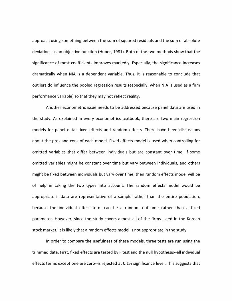
approach using something between the sum of squared residuals and the sum of absolute
deviations as an objective function (Huber, 1981). Both of the two methods show that the
significance of most coefficients improves markedly. Especially, the significance increases
dramatically when NIA is a dependent variable. Thus, it is reasonable to conclude that
outliers do influence the pooled regression results (especially, when NIA is used as a firm
performance variable) so that they may not reflect reality.
Another econometric issue needs to be addressed because panel data are used in
the study. As explained in every econometrics textbook, there are two main regression
models for panel data: fixed effects and random effects. There have been discussions
about the pros and cons of each model. Fixed effects model is used when controlling for
omitted variables that differ between individuals but are constant over time. If some
omitted variables might be constant over time but vary between individuals, and others
might be fixed between individuals but vary over time, then random effects model will be
of help in taking the two types into account. The random effects model would be
appropriate if data are representative of a sample rather than the entire population,
because the individual effect term can be a random outcome rather than a fixed
parameter. However, since the study covers almost all of the firms listed in the Korean
stock market, it is likely that a random effects model is not appropriate in the study.
In order to compare the usefulness of these models, three tests are run using the
trimmed data. First, fixed effects are tested by F test and the null hypothesis--all individual
effects terms except one are zero--is rejected at 0.1% significance level. This suggests that

the fixed effects model is better than the pooled OLS model. Second, random effects are
examined by the Lagrange multiplier (LM) test and the null hypothesis--cross-sectional
variance components are zero--is rejected at 0.1% significance level. This argues in favor
of the random effects model against the pooled data model. Finally, Hausman test is used
to compare fixed effects and random effects and the null hypothesis-- there is no
significant correlation between the individual effects and the regressors--is rejected at
0.1% significance level in this test. This confirms the argument in favor of the fixed effects
model against the random effects model. In sum, the test results confirm that the fixed
effect model is superior to any other models in dealing with the data.
There are large changes in the estimates for CR1 and CUR of Fixed Effects
regressions and Random Effects regressions in the regressions (1) and (2) when EAR is
deleted, which indicates a multicollinearity problem. Thus the estimates for CR1 and CUR
in the regressions (1) and (2) are obtained via a regression that excludes EAR.
In relation to the second hypothesis that a hump-shaped relation exists between
ownership concentration and firm performance, a Ramsey Regression Equation
Specification Error Test (RESET) for the functional form is conducted. The RESET tests
whether nonlinear combinations of the independent variables help explain the dependent
variable (Ramsey, 1969). The test results ( 066.07= −ep for NIA; 162.2< −ep for OIA)
confirm the nonlinear relationship between ownership concentration and firm
performance. In order to test the hump-shaped pattern, piecewise OLS regression and
quadratic OLS regression are run on the trimmed data.
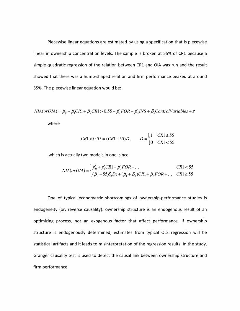
Piecewise linear equations are estimated by using a specification that is piecewise
linear in ownership concentration levels. The sample is broken at 55% of CR1 because a
simple quadratic regression of the relation between CR1 and OIA was run and the result
showed that there was a hump-shaped relation and firm performance peaked at around
55%. The piecewise linear equation would be:
εββββββ ++++++ iablesControlVarINSFORCRCROIAorNIA 543210 0.55>11=)(
where
≥
−55<10
5511=,55)1(=0.55>1
CR
CRDDCRCR
which is actually two models in one, since
≥++++−
+++
5511)()55(
55<11=)(
32120
310
CRFORCRD
CRFORCROIAorNIA
K
K
βββββ
βββ
One of typical econometric shortcomings of ownership-performance studies is
endogeneity (or, reverse causality): ownership structure is an endogenous result of an
optimizing process, not an exogenous factor that affect performance. If ownership
structure is endogenously determined, estimates from typical OLS regression will be
statistical artifacts and it leads to misinterpretation of the regression results. In the study,
Granger causality test is used to detect the causal link between ownership structure and
firm performance.

Results
All of the regression results are shown in Tables 5, 6, 7 and 8.
------------------------------------
Tables 5, 6, 7 and 8 are here.
------------------------------------
The result of the fixed effects regression, which is shown to be superior to other
regressions, provides evidence that ownership concentration has positive effects on firm
performance. The ownership concentration (CR1) has positive and statistically significant
coefficients for each regression: 0.04 ( t =2.71), 0.09 ( t =7.31), 0.04 ( t =2.54), and 0.09
( t =7.20), respectively. For example, according to the result of the regression (4), for 1%
increase in ownership concentration, the ratio of ordinary income to assets increases by
0.09. The result comfirms the positive relaitonship between ownership concentration and
firm performance. Whereas the effect of ownership concentration is confirmed to be
economically and statistically significant, there seems to be no significant relationship
between ownership identity (i.e., foreign ownership and institutional ownership) and firm
performance.
The effects of some control variables on firm performance are confirmed to be
significant in the fixed effects regression. Among control variables, size is noticeable. The
positive effect of firm size (i.e., total assets and total sales) on firm performance is strong
and statistically significant: 1.55 ( t =2.82), 2.94 ( t =6.13), 2.19 ( t =7.27) and 3.04 ( t =11.74).
The regression results indicate that big firms show higher performance. Leverage is also

found to be important in explaining firm performance. The positive relation between the
equity to total assets ratio (EAR) and the dependent variables, and the negative relation
between the liabilities to equity ratio (LER) and the dependent variables are statistically
significant although the coefficients of LER are small: 0.14 ( t =9.79), 0.22 ( t =17.56), -0.00
( t =-5.86) and -0.00 ( t =-8.15). It implies that the higher equity ratio and the lower debt
ratio improve the firm performance. The result supports, at least in part, the view that the
excessively high ratio of debt to equity of Korean firms left corporate sector vulnerable to
the 1997-98 financial crisis. Liquidity also might be a factor in determining firm
performance. Although the coefficients are not significantly different from zero, the
relation between the liquidity variables (CUR and QKR) and the dependent variables is
shown to be statistically significant: 0.00 ( t =3.09), 0.00 ( t =1.67), 0.00 ( t =4.06) and 0.00
( t =3.64).
The results of the piecewise regression and the quadratic regression can be
understood as supporting the idea of the hump-shaped relationship between ownership
concentration and firm performance that the effect of ownership concentration on firm
performance is positive at lower levels of ownership concentration, but negative at higher
levels of ownership concentration. The piecewise regression result shows that firm
performance increases as ownership concentration increases up the point at which
ownership concentration reaches 55%, but decreases slowly after the peak point: the
slopes are 0.10 ( t =8.10), 0.14 ( t =11.81), 0.12 ( t =9.90) and 0.18 ( t =14.23) at low levels of
ownerhsip concentration; -0.04, -0.10, -0.04 and -0.08 at high levels of ownerhsip
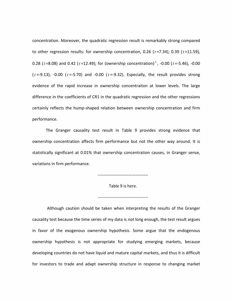
concentration. Moreover, the quadratic regression result is remarkably strong compared
to other regression results: for ownership concentration, 0.26 ( t =7.34), 0.39 ( t =11.59),
0.28 ( t =8.08) and 0.42 ( t =12.49); for (ownership concentration) 2 , -0.00 ( t =-5.46), -0.00
( t =-9.13), -0.00 ( t =-5.70) and -0.00 ( t =-9.32). Especially, the result provides strong
evidence of the rapid increase in ownership concentraiton at lower levels. The large
difference in the coefficients of CR1 in the quadratic regression and the other regressions
certainly reflects the hump-shaped relation between ownership concentration and firm
performance.
The Granger causality test result in Table 9 provides strong evidence that
ownership concentration affects firm performance but not the other way around. It is
statistically significant at 0.01% that ownership concentration causes, in Granger sense,
variations in firm performance.
------------------------------------
Table 9 is here.
------------------------------------
Although caution should be taken when interpreting the results of the Granger
causality test because the time series of my data is not long enough, the test result argues
in favor of the exogenous ownership hypothesis. Some argue that the endogenous
ownership hypothesis is not appropriate for studying emerging markets, because
developing countries do not have liquid and mature capital markets, and thus it is difficult
for investors to trade and adapt ownership structure in response to changing market
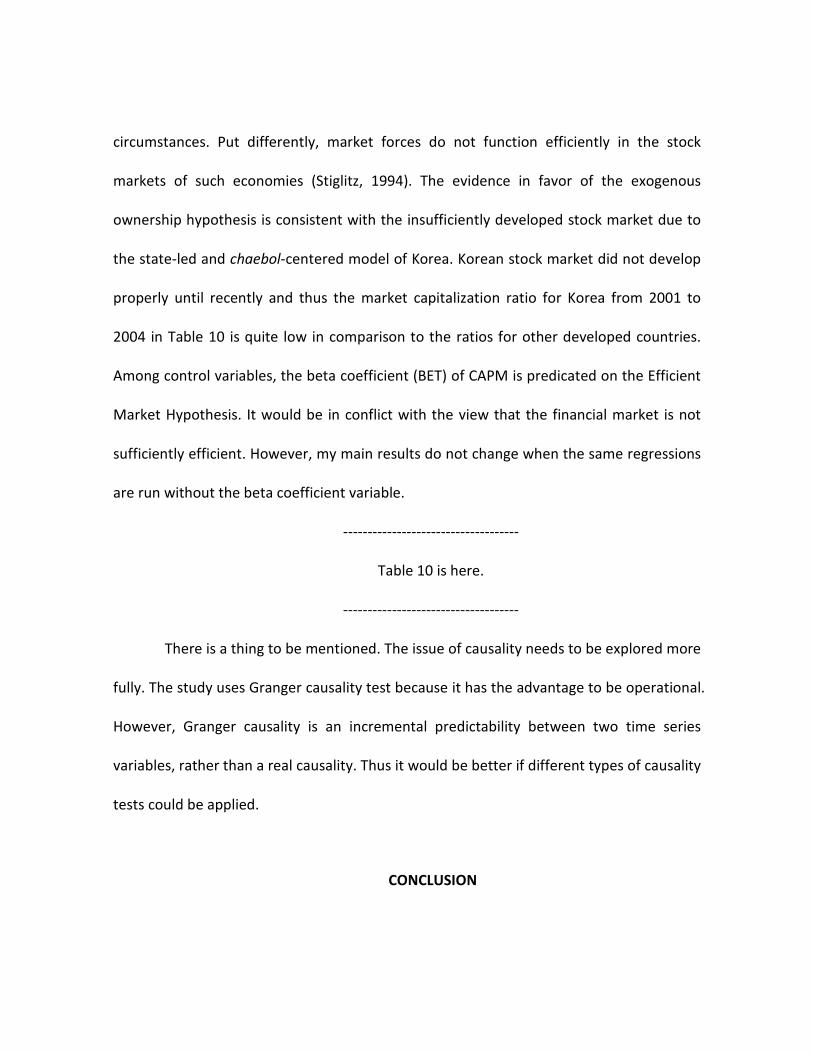
circumstances. Put differently, market forces do not function efficiently in the stock
markets of such economies (Stiglitz, 1994). The evidence in favor of the exogenous
ownership hypothesis is consistent with the insufficiently developed stock market due to
the state-led and chaebol-centered model of Korea. Korean stock market did not develop
properly until recently and thus the market capitalization ratio for Korea from 2001 to
2004 in Table 10 is quite low in comparison to the ratios for other developed countries.
Among control variables, the beta coefficient (BET) of CAPM is predicated on the Efficient
Market Hypothesis. It would be in conflict with the view that the financial market is not
sufficiently efficient. However, my main results do not change when the same regressions
are run without the beta coefficient variable.
------------------------------------
Table 10 is here.
------------------------------------
There is a thing to be mentioned. The issue of causality needs to be explored more
fully. The study uses Granger causality test because it has the advantage to be operational.
However, Granger causality is an incremental predictability between two time series
variables, rather than a real causality. Thus it would be better if different types of causality
tests could be applied.
CONCLUSION
The empirical findings shed light on the role ownership structure plays in firm
performance, and thus offer insights to policy makers interested in improving corporate
governance systems in an emerging economy such as South Korea.
Using panel data for 579 firms in South Korea during 2000--2006, the study finds
that firm performance improves as ownership concentration increases. The result
supports the traditional agency theory and the Granger causality test clearly supports the
exogenous ownership hypothesis. However, unlike previous empirical findings, the effects
of foreign ownership and institutional ownership on firm performance are not significant.
The evidence can be interpreted in the way that the long tradition of state-led economic
development in Korea has made difficult institutional changes allowing for the active role
of foreign investors and ``institutional shareholder activism.'' Indeed, recent discussions
about the corporate governance environment of Korea have suggested that although
corporate governance reform has been conducted in Korea since 1980s and has been
accelerated since the financial crisis in 1997, external mechanisms of corporate
governance such as legal provisions to protect investors and financial markets have not
yet been developed sufficiently (e.g., Kim et al., 2004). As a result, foreign ownership and
institutional ownership are shown not to affect firm performance. The results of positive
effect of ownership concentration and insignificant effect of foreign and institutional
ownership concur with the hypothesis reported by two meta-analyses (Dalton et al., 2003;
Sanchez and Garcia, 2007) that the effect of ownership concentration on firm
performance is more positive and significant where legal protection of investors is weak.

The data also provide strong evidence that there exists a hump-shaped
relationship between ownership concentration and firm performance, in which firm
performance peaks at intermediate levels of ownership concentration. The finding
provides empirical support for the hypothesis that as ownership concentration increases,
the positive monitoring effect of concentrated ownership first dominates but later is
outweighed by the negative effects, such as the expropriation of minority shareholders.
Given substantial ownership concentration in Korean firms, especially chaebols, the
influence of controlling shareholders can lead to the expropriation of minority
shareholders. Although a significant linear relationship between ownership concentration
and firm performance found in the study suggests that concentrated ownership can be an
effective mechanism of corporate governance in a country with limited legal protection of
investors, the nonlinear effect of ownership concentration on firm performance shows the
possibility that controlling shareholders can expropriate wealth from minority
shareholders in such a country.
References
Agrawal, A. and Knoeber, C. R. (1996) Firm Performance and Mechanisms to Control
Agency Problems between Managers and Shareholders. The Journal of Financial and
Quantitative Analysis, 31, 377–397.
Alchian, A. A. and Demsetz, H. (1972) Production, Information Costs, and Economic
Organization. American Economic Review, 62, 777–795.
Baek, J. S., Kang, J. K. and Park, K. S. (2004) Corporate Governance and Firm Value:
Evidence from the Korean Financial Crisis. Journal of Financial Economics, 71, 265–313.
Bergstr¨om, C. and Rydqvist, K. (1990) The Determinants of Corporate Ownership: An
Empirical Study on Swedish Data. Journal of Banking and Finance, 14, 237–253.
Berle, A. and Means, G. (1932) The Modern Corporation and Private Property. New York,
NY: Macmillan.
Black, B. S. (1998) Shareholder Activism and Corporate Governance in the U.S. In P.
Newman (ed.) The New Palgrave Dictionary of Economics and the Law. Macmillan.
Cho, M.-H. (1998) Ownership Structure, Investment, and The Corporate Value: An
Empirical Analysis. Journal of Financial Economics, 47, 103–121.
Claessens, S., Djankov, S., Fan, J. P. H. and Lang, L. H. P. (2002) Disentangling the Incentive
and Entrenchment Effects of Large Shareholdings. Journal of Finance, 57, 2741–2772.
Claessens, S., Djankov, S. and Xu, L. C. (2000) Corporate Performance in the East Asian
Financial Crisis. The World Bank Research Observer, 15, 23–46.
Coase, R. H. (1937) The Nature of the Firm. Economica, 4, 386–405.
Dalton, D. R., Daily, C. M., Certo, S. T. and Roengpitya, R. (2003) Meta-Analyses of
Financial Performance and Equity: Fusion or Confusion? Academy of Management Journal,
46, 13–26.
Demsetz, H. (1983) The Structure of Ownership and the Theory of the Firm. Journal of Law
and Economics, 26, 375–390.
Demsetz, H. and Lehn, K. (1985) The Structure of Corporate Ownership: Causes and
Consequences. The Journal of Political Economy, 93, 1155–1177.

Demsetz, H. and Villalonga, B. (2001) Ownership Structure and Corporate Performance.
Journal of Corporate Finance, 7, 209–233.
Gel, Y. R. and Gastwirth, J. L. (2006) A Robust Modification of the Jarque-Bera Test of
Normality. Working Paper.
Gillan, S. L. and Starks, L. T. (1998) A Survey of Shareholder Activism: Motivation and
Empirical Evidence. Contemporary Finance Digest, 2, 10–34.
Gugler, K. (2001) Corporate Governance and Economic Performance. New York: Oxford
University Press.
Hermalin, B. E. and Weisbach, M. S. (1991) The Effects of Board Composition and Direct
Incentives on Firm Performance. Financial Management, 20, 101–112.
Himmelberg, C. P., Hubbard, R. G. and Palia, D. (1999) Understanding the Determinants of
Managerial Ownership and the Link between Ownership and Performance. Journal of
Financial Economics, 53, 353–384.
Holderness, C. G. and Sheehan, D. P. (1988) The Role of Majority Shareholders in
Publicly-held Corporations. Journal of Financial Economics, 20, 317–346.
Huber, P. J. (1973) Robust Regression: Asymptotics, Conjectures and Monte Carlo. The
Annals of Statistics, 1, 799–821.
Huber, P. J. (1981) Robust Statistics. New York: John Wiley and Sons.
Jarque, C. M. and Bera, A. K. (1980) Efficient Tests for Normality, Homoscedasticity and
Serial Independence of Regression Residuals. Econometric Letters, 6, 255–259.
Joh, S. W. (2003) Corporate Governance and Firm Profitability: Evidence from Korea
Before the Economic Crisis. Journal of Financial Economics, 68, 287–322.
Kim, E. H. and Kim, W. (2008) Changes in Korean Corporate Governance: A Response to
Crisis. Journal of Applied Corporate Finance, 20, 47–58.
Kim, H. S., Kim, N. S. and Wong, C. (2004) Korea. In G. S. Dallas (ed.) Governance and Risk:
An Analytical Handbook for Investors, Managers, Directors, and Stakeholders. New York,
NY: McGraw-Hill.
Lins, K. V. (2003) Equity Ownership and Firm Value in Emerging Markets. Journal of
Financial and Quantitative Analysis, 38, 159–184.
McConnell, J. J. and Servaes, H. (1990) Additional Evidence on Equity Ownership and
Corporate Value. Journal of Financial Economics, 27, 595–612.
Mitton, T. (2002) A Cross-Firm Analysis of the Impact of Corporate Governance on the East
Asian Financial Crisis. Journal of Financial Economics, 64, 215–241.
Morck, R., Shleifer, A. and Vishny, R. (1988) Management Ownership and Market
Valuation: An Empirical Analysis. Journal of Financial Economics, 20, 293–315.
Owen, G., Kirchmaier, T. and Grant, J. (eds.) (2005) Corporate Governance in the US and
Europe: Where Are We Now? New York, NY: Palgrave Macmillan.
Oxelheim, L. and Randøy, T. (2003) The Impact of Foreign Board Membership on Firm
Value. Journal of Banking and Finance, 27, 2369–2392.
Park, Y. S. (2004) Assessing The Impact Of Corporate Governance On Productivity And
Growth In Korea. In E. T. Gonzalez (ed.) Impact of Corporate Governance on Productivity:
Asian Experience. Asian Productivity Organization.
Porta, R. L., de Silanes, F. L. and Shleifer, A. (1999) Corporate Ownership Around theWorld.
The Journal of Finance, 54, 471–517.
Ramsey, J. B. (1969) Tests for Specification Errors in Classical Linear Least Squares
Regression Analysis. Journal of the Royal Statistical Society. Series B (Methodological), 31,
350–371.
Romano, R. (2001) Less is More: Making Institutional Investor Activism a Valuable
Mechanism of Corporate Governance. Yale Journal on Regulation, 18, 174–251.
Sanchez-Ballesta, J. P. and Garcıa-Meca, E. (2007) A Meta-Analytic Vision of the Effect of
Ownership Structure on Firm Performance. Corporate Governance, 15, 879–893.
Scott, J. (1986) Capitalist Property and Financial Power: A Comparative Study of Britain,
the United States and Japan. Brighton: Wheatsheaf.
Shapiro, S. S. and Wilk, M. B. (1965) An Analysis of Variance Test for Normality (Complete
Samples). Biometrika, 52, 591–611.
Shleifer, A. and Vishny, R. (1997) A Survey of Corporate Governance. Journal of Finance, 52,
737–783.
Short, H. (1994) Ownership, Control, Financial Structure and the Performance of Firms.
Journal of Economic Surveys, 8, 203–249.
Short, H. and Keasey, K. (1999) Managerial Ownership and the Performance of Firms:
Evidence from the U.K. Journal of Corporate Finance, 5, 79–101.
Stiglitz, J. E. (1994) Whither Socialism? Cambridge, Massachusetts: MIT Press.
Thomsen, S. and Pedersen, T. (2000) Ownership Structure and Economic Performance in
the Largest European Companies. Strategic Management Journal, 21, 689–705.

Table 1: Description of Variables and Summary Statistics
Variable Name Description Min Median Mean Max
Ownership
Concentration
CR1 The percentage of
shares held by the
largest shareholder
0.00 37.87 38.54 100.00
Foreign
Ownership
FOR The percentage of
shares held by foreign
owners
0.00 2.08 9.89 99.89
Institutional
Ownership
INS The percentage of
shares held by
institutional investors
0.00 4.74 9.97 95.31
Size LNA Natural Logarithm of
Total Assets
2.83 7.51 7.73 13.37
LNS Natural Logarithm of
Total Sales
-1.20 7.29 7.47 13.26
Leverage EAR Equity to Total Assets
Ratio
0.24 52.18 51.94 98.40
LER Liabilities to Equity
Ratio
0.00 91.58 196.20 40990.72
Liquidity CUR Current (Assets to
Liabilities) Ratio
1.18 132.72 175.86 4473.67
QKR Quick Ratio 1.18 96.85 133.68 4473.67
Risk BET Beta Coefficient of the
capital asset pricing
model (CAPM)
-0.38 0.64 0.65 2.00
Business
Cycle
IVA Inventory to Total
Assets Ratio
0.00 0.09 0.11 2.86
BCL Business Cycle
Dummy
Industry IDS Industry Dummies
Performance NIA Net Income to Total
Assets Ratio
-938.53 3.50 3.51 2357.53
OIA Ordinary Income to
Total Assets Ratio
-928.78 4.21 3.08 77.78
The table shows the description of variables and summary statistics for the variables. This
is a balanced panel of 579 firms, for which there are available annual observations for the
period 2000-2006. The total number of observations is 4053.
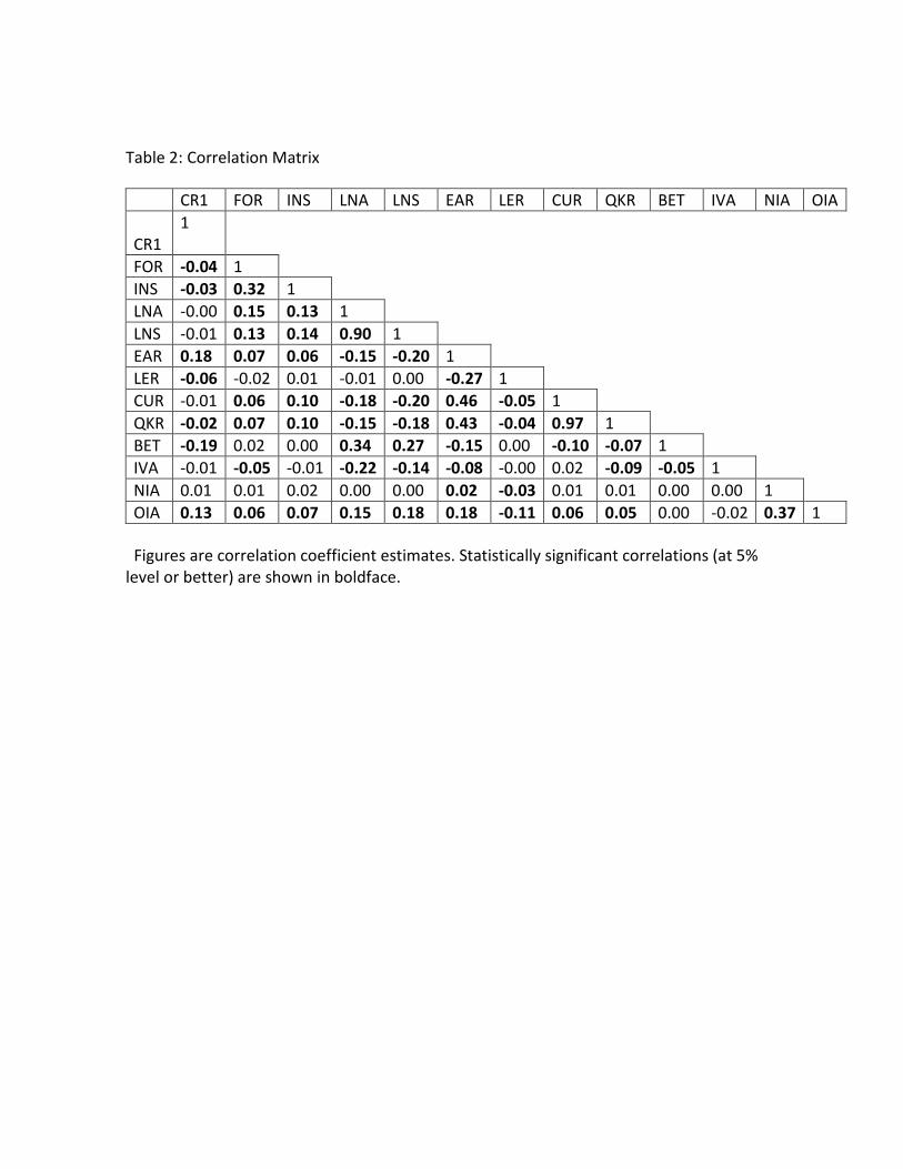
Table 2: Correlation Matrix
CR1 FOR INS LNA LNS EAR LER CUR QKR BET IVA NIA OIA
CR1
1
FOR -0.04 1
INS -0.03 0.32 1
LNA -0.00 0.15 0.13 1
LNS -0.01 0.13 0.14 0.90 1
EAR 0.18 0.07 0.06 -0.15 -0.20 1
LER -0.06 -0.02 0.01 -0.01 0.00 -0.27 1
CUR -0.01 0.06 0.10 -0.18 -0.20 0.46 -0.05 1
QKR -0.02 0.07 0.10 -0.15 -0.18 0.43 -0.04 0.97 1
BET -0.19 0.02 0.00 0.34 0.27 -0.15 0.00 -0.10 -0.07 1
IVA -0.01 -0.05 -0.01 -0.22 -0.14 -0.08 -0.00 0.02 -0.09 -0.05 1
NIA 0.01 0.01 0.02 0.00 0.00 0.02 -0.03 0.01 0.01 0.00 0.00 1
OIA 0.13 0.06 0.07 0.15 0.18 0.18 -0.11 0.06 0.05 0.00 -0.02 0.37 1
Figures are correlation coefficient estimates. Statistically significant correlations (at 5%
level or better) are shown in boldface.
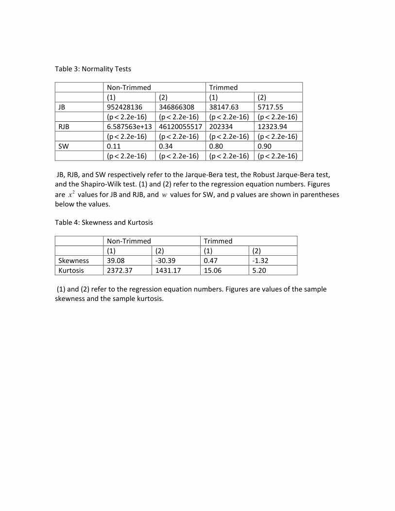
Table 3: Normality Tests
Non-Trimmed Trimmed
(1) (2) (1) (2)
JB 952428136 346866308 38147.63 5717.55
(p < 2.2e-16) (p < 2.2e-16) (p < 2.2e-16) (p < 2.2e-16)
RJB 6.587563e+13 46120055517 202334 12323.94
(p < 2.2e-16) (p < 2.2e-16) (p < 2.2e-16) (p < 2.2e-16)
SW 0.11 0.34 0.80 0.90
(p < 2.2e-16) (p < 2.2e-16) (p < 2.2e-16) (p < 2.2e-16)
JB, RJB, and SW respectively refer to the Jarque-Bera test, the Robust Jarque-Bera test,
and the Shapiro-Wilk test. (1) and (2) refer to the regression equation numbers. Figures
are 2
x values for JB and RJB, and w values for SW, and p values are shown in parentheses
below the values.
Table 4: Skewness and Kurtosis
Non-Trimmed Trimmed
(1) (2) (1) (2)
Skewness 39.08 -30.39 0.47 -1.32
Kurtosis 2372.37 1431.17 15.06 5.20
(1) and (2) refer to the regression equation numbers. Figures are values of the sample
skewness and the sample kurtosis.
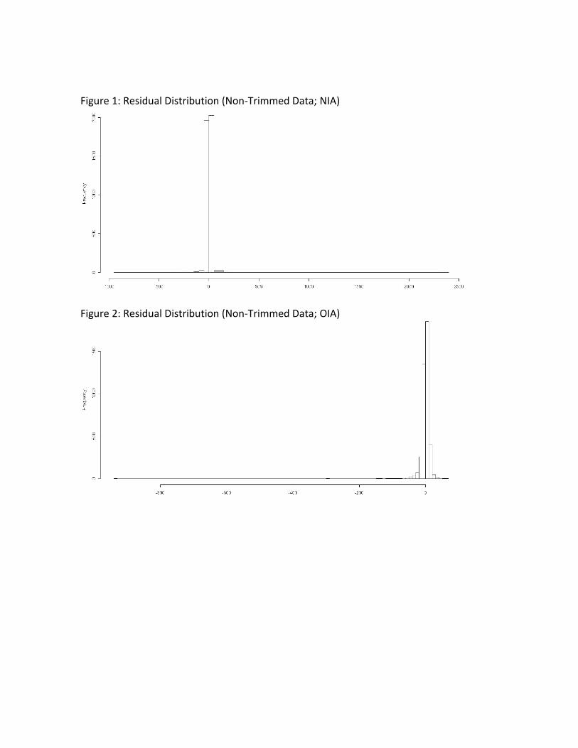
Figure 1: Residual Distribution (Non-Trimmed Data; NIA)
Figure 2: Residual Distribution (Non-Trimmed Data; OIA)

Figure 3: Residual Distribution (Trimmed Data; NIA)
Figure 4: Residual Distribution (Trimmed Data; OIA)
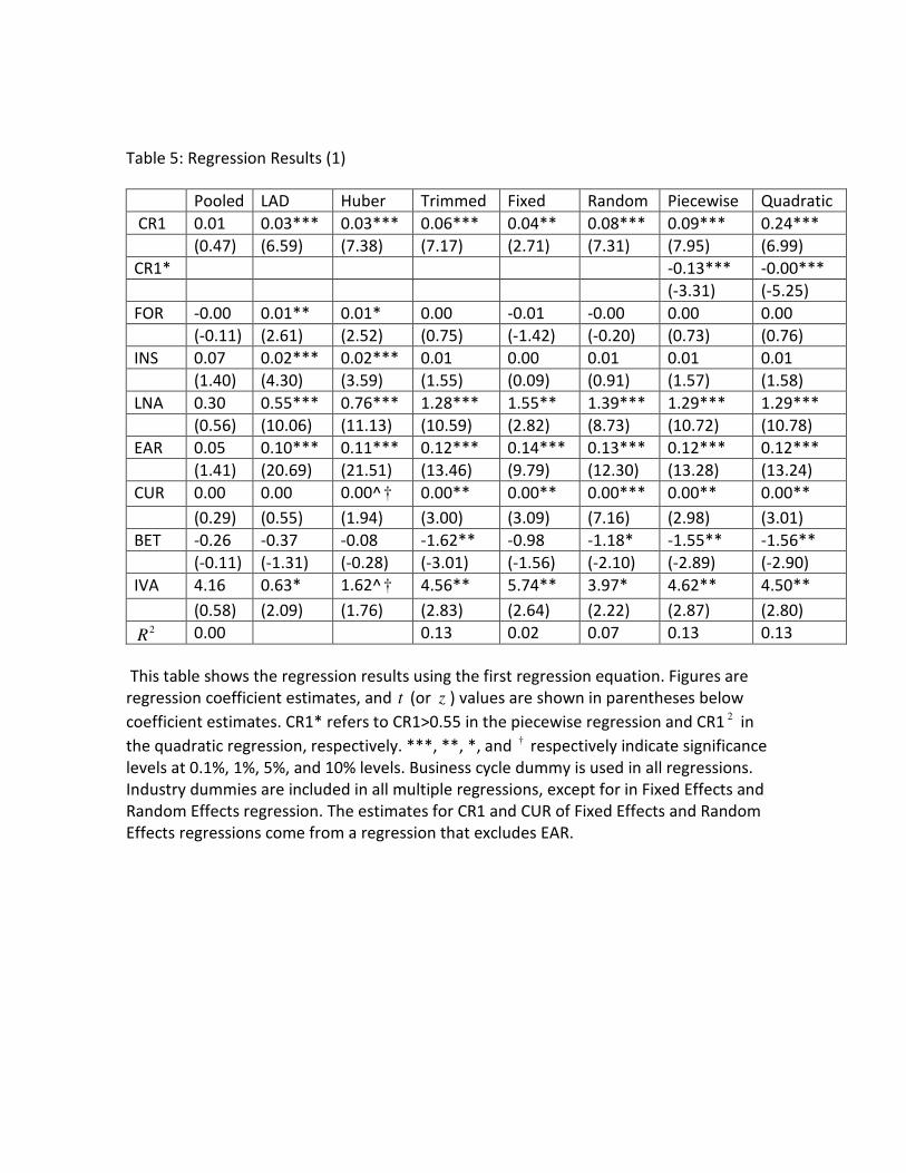
Table 5: Regression Results (1)
Pooled LAD Huber Trimmed Fixed Random Piecewise Quadratic
CR1 0.01 0.03*** 0.03*** 0.06*** 0.04** 0.08*** 0.09*** 0.24***
(0.47) (6.59) (7.38) (7.17) (2.71) (7.31) (7.95) (6.99)
CR1* -0.13*** -0.00***
(-3.31) (-5.25)
FOR -0.00 0.01** 0.01* 0.00 -0.01 -0.00 0.00 0.00
(-0.11) (2.61) (2.52) (0.75) (-1.42) (-0.20) (0.73) (0.76)
INS 0.07 0.02*** 0.02*** 0.01 0.00 0.01 0.01 0.01
(1.40) (4.30) (3.59) (1.55) (0.09) (0.91) (1.57) (1.58)
LNA 0.30 0.55*** 0.76*** 1.28*** 1.55** 1.39*** 1.29*** 1.29***
(0.56) (10.06) (11.13) (10.59) (2.82) (8.73) (10.72) (10.78)
EAR 0.05 0.10*** 0.11*** 0.12*** 0.14*** 0.13*** 0.12*** 0.12***
(1.41) (20.69) (21.51) (13.46) (9.79) (12.30) (13.28) (13.24)
CUR 0.00 0.00 0.00^† 0.00** 0.00** 0.00*** 0.00** 0.00**
(0.29) (0.55) (1.94) (3.00) (3.09) (7.16) (2.98) (3.01)
BET -0.26 -0.37 -0.08 -1.62** -0.98 -1.18* -1.55** -1.56**
(-0.11) (-1.31) (-0.28) (-3.01) (-1.56) (-2.10) (-2.89) (-2.90)
IVA 4.16 0.63* 1.62^† 4.56** 5.74** 3.97* 4.62** 4.50**
(0.58) (2.09) (1.76) (2.83) (2.64) (2.22) (2.87) (2.80) 2R 0.00 0.13 0.02 0.07 0.13 0.13
This table shows the regression results using the first regression equation. Figures are
regression coefficient estimates, and t (or z ) values are shown in parentheses below
coefficient estimates. CR1* refers to CR1>0.55 in the piecewise regression and CR1 2 in
the quadratic regression, respectively. ***, **, *, and † respectively indicate significance
levels at 0.1%, 1%, 5%, and 10% levels. Business cycle dummy is used in all regressions.
Industry dummies are included in all multiple regressions, except for in Fixed Effects and
Random Effects regression. The estimates for CR1 and CUR of Fixed Effects and Random
Effects regressions come from a regression that excludes EAR.

Table 6: Regression Results (2)
Pooled LAD Huber Trimmed Fixed Random Piecewise Quadratic
CR1 0.11*** 0.04*** 0.05*** 0.08*** 0.09*** 0.11*** 0.13*** 0.36***
(6.21) (7.05) (8.33) (9.48) (7.31) (10.15) (11.08) (11.17)
CR1* -0.22*** -0.00***
(-5.93) (-8.91)
FOR 0.01 0.02** 0.01* 0.01 -0.02* -0.01 0.01 0.01
(0.89) (3.19) (2.40) (1.46) (-2.33) (-0.97) (1.42) (1.47)
INS 0.05* 0.03*** 0.04*** 0.04*** 0.01 0.02^† 0.04*** 0.04***
(2.44) (4.99) (4.47) (3.60) (0.86) (1.86) (3.63) (3.67)
LNA 2.41*** 0.91*** 1.15*** 1.65*** 2.94*** 1.89*** 1.67*** 1.67***
(10.16) (11.31) (13.16) (14.27) (6.13) (10.68) (14.50) (14.60)
EAR 0.19*** 0.14*** 0.16*** 0.18*** 0.22*** 0.20*** 0.18*** 0.18***
(10.70) (22.60) (24.23) (21.14) (17.56) (19.42) (20.90) (20.93)
CUR -0.00 0.00 0.00 0.00 0.00^† 0.00*** 0.00 0.00
(-0.38) (0.65) (0.25) (0.15) (1.67) (4.99) (0.10) (0.13)
BET -0.84 -0.27 0.19 -0.58 0.74 0.29 -0.46 -0.46
(-0.79) (-0.71) (0.48) (-1.14) (1.39) (0.56) (-0.90) (-0.90)
IVA 8.61** 1.29 2.23^† 3.88* 5.43** 4.56* 3.91* 3.72*
(2.69) (0.98) (1.89) (2.44) (2.79) (2.57) (2.47) (2.36) 2R 0.08 0.21 0.09 0.12 0.22 0.23
This table shows the regression results using the second regression equation. Figures are
regression coefficient estimates, and t (or z ) values are shown in parentheses below
coefficient estimates. CR1* refers to CR1>0.55 in the piecewise regression and CR1 2 in
the quadratic regression, respectively. ***, **, *, and † respectively indicate significance
levels at 0.1%, 1%, 5%, and 10% levels. Business cycle dummy is used in all regressions.
Industry dummies are included in all multiple regressions, except for in Fixed Effects and
Random Effects regression. The estimates for CR1 and CUR of Fixed Effects and Random
Effects regressions come from a regression that excludes EAR.
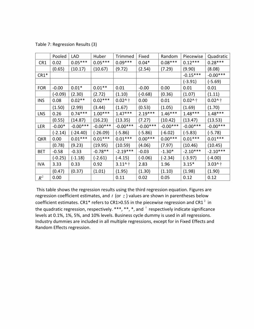
Table 7: Regression Results (3)
Pooled LAD Huber Trimmed Fixed Random Piecewise Quadratic
CR1 0.02 0.05*** 0.05*** 0.09*** 0.04* 0.08*** 0.12*** 0.28***
(0.65) (10.17) (10.67) (9.72) (2.54) (7.29) (9.90) (8.08)
CR1* -0.15*** -0.00***
(-3.91) (-5.69)
FOR -0.00 0.01* 0.01** 0.01 -0.00 0.00 0.01 0.01
(-0.09) (2.30) (2.72) (1.10) (-0.68) (0.36) (1.07) (1.11)
INS 0.08 0.02** 0.02*** 0.02^† 0.00 0.01 0.02^† 0.02^†
(1.50) (2.99) (3.44) (1.67) (0.53) (1.05) (1.69) (1.70)
LNS 0.26 0.74*** 1.00*** 1.47*** 2.19*** 1.46*** 1.48*** 1.48***
(0.55) (14.87) (16.23) (13.35) (7.27) (10.42) (13.47) (13.53)
LER -0.00* -0.00*** -0.00*** -0.00*** -0.00*** -0.00*** -0.00*** -0.00***
(-2.14) (-24.40) (-26.09) (-5.86) (-5.86) (-6.02) (-5.83) (-5.78)
QKR 0.00 0.01*** 0.01*** 0.01*** 0.00*** 0.00*** 0.01*** 0.01***
(0.78) (9.23) (19.95) (10.59) (4.06) (7.97) (10.46) (10.45)
BET -0.58 -0.33 -0.78** -2.19*** -0.03 -1.30* -2.10*** -2.10***
(-0.25) (-1.18) (-2.61) (-4.15) (-0.06) (-2.34) (-3.97) (-4.00)
IVA 3.33 0.33 0.92 3.11^† 2.83 1.96 3.15* 3.03^†
(0.47) (0.37) (1.01) (1.95) (1.30) (1.10) (1.98) (1.90) 2R 0.00 0.11 0.02 0.05 0.12 0.12
This table shows the regression results using the third regression equation. Figures are
regression coefficient estimates, and t (or z ) values are shown in parentheses below
coefficient estimates. CR1* refers to CR1>0.55 in the piecewise regression and CR1 2 in
the quadratic regression, respectively. ***, **, *, and † respectively indicate significance
levels at 0.1%, 1%, 5%, and 10% levels. Business cycle dummy is used in all regressions.
Industry dummies are included in all multiple regressions, except for in Fixed Effects and
Random Effects regression.

Table 8: Regression Results (4)
Pooled LAD Huber Trimmed Fixed Random Piecewise Quadratic
CR1 0.14*** 0.06*** 0.08*** 0.11*** 0.09*** 0.11*** 0.17*** 0.41***
(8.08) (10.43) (12.19) (13.01) (7.20) (10.09) (14.22) (12.49)
CR1* -0.25*** -0.00***
(-6.64) (-9.31)
FOR 0.02 0.01* 0.02** 0.02* -0.00 0.00 0.02* 0.02*
(1.19) (2.40) (2.57) (2.05) (-0.82) (0.15) (2.02) (2.07)
INS 0.06* 0.03*** 0.03*** 0.04*** 0.02^† 0.02* 0.04*** 0.04***
(2.47) (4.42) (4.37) (3.85) (1.69) (2.23) (3.88) (3.92)
LNS 2.70*** 1.14*** 1.43*** 1.81*** 3.04*** 1.95*** 1.82*** 1.82***
(12.70) (15.69) (17.92) (16.94) (11.74) (12.91) (17.16) (17.24)
LER -0.00*** -0.00^† -0.00*** -0.00*** -0.00*** -0.00*** -0.00*** -0.00***
(-6.37) (-1.93) (-21.57) (-9.02) (-8.15) (-8.53) (-9.00) (-8.96)
QKR 0.00*** 0.01*** 0.01*** 0.01*** 0.00*** 0.00*** 0.01*** 0.01***
(4.97) (10.39) (18.73) (11.11) (3.64) (6.46) (10.91) (10.92)
BET -1.78^† -0.38 -0.61 -1.25* 2.25*** 0.60 -1.07* -1.08*
(-1.72) (-1.09) (-1.57) (-2.44) (4.16) (1.16) (-2.10) (-2.13)
IVA 4.85 0.72^† 0.71 0.54 -0.58 0.27 0.55 0.36
(1.54) (1.87) (0.60) (0.34) (-0.29) (0.15) (0.34) (0.22) 2R 0.08 0.17 0.06 0.08 0.18 0.19
This table shows the regression results using the fourth regression equation. Figures are
regression coefficient estimates, and t (or z ) values are shown in parentheses below
coefficient estimates. CR1* refers to CR1>0.55 in the piecewise regression and CR1 2 in
the quadratic regression, respectively. ***, **, *, and † respectively indicate significance
levels at 0.1%, 1%, 5%, and 10% levels. Business cycle dummy is used in all regressions.
Industry dummies are included in all multiple regressions, except for in Fixed Effects and
Random Effects regression.
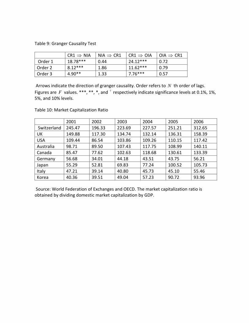
Table 9: Granger Causality Test
CR1 ⇒ NIA NIA ⇒ CR1 CR1 ⇒ OIA OIA ⇒ CR1
Order 1 18.78*** 0.44 24.12*** 0.72
Order 2 8.12*** 1.86 11.62*** 0.79
Order 3 4.90** 1.33 7.76*** 0.57
Arrows indicate the direction of granger causality. Order refers to N th order of lags.
Figures are F values. ***, **, *, and † respectively indicate significance levels at 0.1%, 1%,
5%, and 10% levels.
Table 10: Market Capitalization Ratio
2001 2002 2003 2004 2005 2006
Switzerland 245.47 196.33 223.69 227.57 251.21 312.65
UK 149.88 117.30 134.74 132.14 136.31 158.39
USA 109.44 86.54 103.86 109.26 110.15 117.42
Australia 98.71 89.50 107.43 117.75 108.99 140.11
Canada 85.47 77.62 102.63 118.68 130.61 133.39
Germany 56.68 34.01 44.18 43.51 43.75 56.21
Japan 55.29 52.81 69.83 77.24 100.52 105.73
Italy 47.21 39.14 40.80 45.73 45.10 55.46
Korea 40.36 39.51 49.04 57.23 90.72 93.96
Source: World Federation of Exchanges and OECD. The market capitalization ratio is
obtained by dividing domestic market capitalization by GDP.