ownership concentration measures compared
TRANSCRIPT

1
Keeping it real or keeping it simple?
Ownership concentration measures compared
January, 2012
Conny Overlanda,b
Taylan Mavruka,c
Stefan Sjögrena,d
University of Gothenburg
Abstract Based on a sample of 240 Swedish firms listed at the Stockholm Stock Exchange as of year-end 2008 we analyze measures of ownership concentration found in past governance literature. We find that although measures are significantly correlated, they show different distributional properties. We also identify the best underlying distribution for each concentration measure, and we are able to distinguish between measures in terms of what dimensions of ownership they describe. Finally, we document that inferences regarding the association between ownership concentration and firm performance are contingent on the choice of concentration measure. JEL-codes: C18, C46, C81, D74, G34, L25,
Keywords: Ownership concentration measures, distributional properties, Sweden
a University of Gothenburg, Department of Business Administration, Box 610, SE-405 30 Gothenburg b Phone: +46-31-786 12 72, E-mail: [email protected] c Phone: +46-31-786 59 58, E-mail: [email protected] d Phone: +46-31-786 14 99, E-mail: [email protected] We thank Roger Wahlberg, Ted Lindblom, Mattias Hamberg, Evert Carlsson and Tamir Agmon for valuable comments and advice. We gratefully aknowledge Euroclear and SIS Ägarservice for providing with data, as well as Dennis Leech for making available the power index algorithms on his webpage.
2
I. Introduction
In studies on the linkage between ownership and what corporations do there is a multitude of
ways to measure ownership concentration. Measures range from simple proxies such as the
largest owner’s voting share, to the computation of advanced power indices based in game
theory. This gives rise to questioning the comparability of such studies. It is especially
problematic if the conclusions diverge between studies adopting different ownership
concentration measures. Then it is important to examine whether and, in that case, why the
choice of concentration measure drives the results of these studies. In particular, knowledge is
needed on whether the simple measures found in most empirical research are sufficient to
capture the role of ownership, or if more theoretically elaborated power indices are necessary.
In this paper we therefore analyze a majority of the various measures of ownership
concentration—in total twenty measures—that have been used in previous research.
To illustrate the problem at hand, the relationship between ownership concentration and firm
performance has been the topic of many studies. In many cases these studies yield conflicting
results. For instance, Morck et al. (2000), Thomsen and Pedersen (2000) and Gedajlovic and
Shapiro (2002) document a positive relationship between ownership concentration and firm
performance, whereas Leech and Leahy (1991), Lehmann and Weigand (2000) and, to some
degree, Claessens et al. (2002)1 find that ownership concentration is negatively related to firm
performance. Other studies, like McConnell and Servaes, (1990) and De Miguel et al. (2004),
find evidence of a nonlinear relationship between ownership concentration and firm
performance. Additionally, studies have documented mixed evidence between countries
(Gedajlovic and Shapiro, 1998) or no significant relationship at all (Demsetz and Villalonga,
1 They find a positive association between cash flow rights and firm value, but a negative relationship between voting rights and firm value.
3
2001). The lack of accordance between studies is a source of uncertainty when exploring how
ownership concentration and firm performance are related. An explanation is warranted to
why conclusions diverge. We are able to distinguish three major reasons to why results differ
between studies: differences in contextual settings, differences in data quality and differences
in methodology.
Differences in contextual settings are present when comparing studies that are based on data
from different countries and time periods. In studies aiming at examining the linkage between
ownership and firm performance differences in legal investor protection (LaPorta et al., 2002)
or extralegal institutions (Dyck and Zingales, 2004) are likely to be vital for the outcome.
Results from an investigation on UK data (Leech and Leahy, 1991) probably differ, at least
partly, from a study on Japanese data (Gedajlovic and Shapiro, 2002). In countries with legal
systems that to a lesser degree discipline managers, an increase in ownership concentration is
likely to add value through better monitoring. Accordingly, the marginal value added from
better monitoring is relatively smaller in countries with more strongly enforced fiduciary
duties. In such countries increases in ownership concentration could instead be associated
with value destruction if gains from better monitoring are outweighed by increases in private
rent extraction by large shareholders.
Differences in ownership data are often associated with problems of incompleteness or
inability to trace ultimate ownership. Data is typically truncated as only large shareholders are
disclosed. For instance, Franks and Mayer (2001) report that in Germany disclosure of owners
that holds less than 25 percent of the stock of the firm is not compulsory, and in their study
such owners are accounted for only when voluntarily disclosed. Countries with more
exhaustive disclosure rules also show similar limitations. Students of US firms must settle
with the disclosure of owners holding five percent or more as reported in SEC filings
(Mehran, 1995; Bauguess et al., 2009), and the corresponding UK cut off is three percent

4
(Leech, 2002). Equivalent limitations are found in most Western European (Faccio and Lang,
2002) and East Asian countries (Claessens et al., 2000). Moreover, ownership data typically
does not allow to trace ultimate ownership through control enhancing mechanisms (CEMs),
which may result in research based on nominal (as opposed to beneficial) ownership (e.g.
Leech, 1988), or a non-randomly reduced sample (e.g. Leech and Leahy, 1991; Leech, 2002;
Edwards and Weichenrieder, 2009).
Differences in methodology are to a great extent due to the choice of different ownership
concentration measures in regression models. A common way to measure ownership
concentration is to take the share held by the largest shareholder (e.g. Thomsen and Pedersen,
2000) or the combined share held by a number of the largest owners (McConnel and Servaes,
1990; Demsetz and Villalonga, 2001; Gedajlovic and Shapiro, 2002; De Miguel et al., 2004).
Other concentration measures include Herfindahl indices (Cubbin and Leech, 1983; Demsetz
and Lehn, 1985; Leech and Leahy, 1991) and measures based in game theory (Rydqvist,
1996; Zingales, 1994, 1995). The results differ among several of these studies. It is
problematic if these differences depend on the choice of ownership concentration measure.
There are few empirical studies on what impact this choice has on the outcome of a study of
the role of ownership. A more in-depth understanding of existent measures of ownership
concentration is necessary for better evaluations and interpretations of the results of previous
studies on ownership effects in corporations.
Part of the explanation to why different ownership concentration measures could lead to
different results may be that these measures have different underlying distributional
properties. Parametric tests require that changes are drawn from a common distribution,
usually a normal distribution, with a finite variance. Test statistics that are used to make
inferences about the effect of ownership concentration are based on the normal distribution, or
on distributions that are closely related to the normal one (such as t, F, or Chi-square). These

5
tests require that the measures analyzed meet the normality assumption. Since the
distributions of ownership concentration measures rarely satisfy the normality assumption,
one reason for obtaining different results, when using different measures, could be related to
the distributional properties of these measures. That distributions actually do differ among
ownership concentration measures is supported by Edwards and Weichenrieder (2009) when
they reject the null hypothesis of equal distributions.
Another possible explanation to why results could be contingent on the choice of ownership
concentration measure is that these measures often capture different dimensions of ownership.
There are at least two potential causes of conflict related to ownership structure that may
affect decision making in firms. One has to do with the relationship between managers and
owners, and the other with the relationship among owners. Starting with the influential paper
by Jensen and Meckling (1976), ample literature claims that managers are more concerned
with maximizing their own utility rather than that of their principals, giving rise to agency
costs. Such agency costs could be dampened through increases in ownership concentration,
because it increases the incentives for large shareholders to engage in costly monitoring. We
call this the monitoring dimension. However, conflicting interests among owners could curb
firm performance as well, where an increase in ownership concentration increases the scope
for large shareholders’ expropriation of minority shareholders (Shleifer and Vishny, 1997;
Burkart et al., 1997; Claessens et al. 2002). We call this the shareholder conflict dimension.
A measure of ownership concentration could possibly be a suitable proxy for analyzing one of
the two dimensions, but a worse proxy for the other dimension. For instance, if the analysis
centers the monitoring dimension the voting share held by the largest owner appears to be a
reasonable proxy for concentration. In this situation the largest shareholder will represent all
shareholders because self-dealing managers are in the best interest of no shareholder. If,
instead, the focal point is the shareholder conflict dimension, it is not necessarily so that a

6
measure of the largest shareholder will contain satisfactory information. Even though the
largest shareholder’s opportunity to extract private rent is augmented by a larger voting share,
it is also affected by the influence of other shareholders. Thus, previous research may in fact
study different phenomena despite claiming to study the same one. This would further drive
the divergence in results among studies.
Based on a sample of all Swedish companies listed at the Stockholm Stock Exchange (SSE)2
as of 31 December 2008, we empirically analyze if different ownership concentration
measures used in previous research. By holding the contextual setting fixed and by using the
best possible data set, we aim to increase our understanding of how the choice of ownership
concentration measures affects results in empirical research. We limit the data set to include
only one country and a limited time period. Thus, contextual differences are mitigated as all
observations are subject to the same legal and extra-legal institutions, as well as the same
time-specific macro events. Data quality problems are avoided as we base our analysis on a
data set free from incompleteness, and free from non-random reductions in sample size. By
minimizing the problems of diverse contexts and data quality we enhance the possibility to
analyze the effects of measurement choices in isolation.
Specifically, we carry out five distinct analyses. First, we investigate, using the Spearman
rank correlation test, whether ownership concentration measures rank firms differently. It is
not unusual that high correlation coefficients are used as an argument for substituting one
measure for another, and therefore we do this test first. Next, we explore the distributional
properties of the measures. This is done through two tests; we test whether distributions of the
concentration measures come from the same distributions using the Wilcoxon matched-pair
signed-ranks test, and we determine what distribution that best fits each measurement using
2 NASDAQ OMX Stockholm

7
the Anderson-Darling test. Thereafter, through principal component analysis (PCA), we
examine whether the two dimensions discussed above are discernable in the underlying
components. Finally, we regress firm performance, in terms of both market-to-book (MTB)
and return on assets (ROA), using alternative ownership concentration measures in order to
illustrate how analytical outcomes can be affected by differences in methodology.
First, we find that all ownership concentration measures are significantly correlated at the five
percent level, albeit their coefficients differ in size. However, the fact that measures correlate
does not imply that the measures are substitutes. One reason for this is that they also show
different underlying distributions. The Wilcoxon tests reject the null hypothesis of equal
median values for the majority of the pairs of concentration measures. Moreover, the
Anderson-Darling tests reveal that, for the 20 different measures considered, we find no less
than 13 different distribution assumptions that best describes the distributional properties of a
specific concentration measure. All but one of the measures in our sample can be rejected to
be normally distributed. However, some of the other measures fall into distributions closely
related to the normal.
Second, we observe that the PCA does not indicate that the ownership concentration measures
studied should be grouped into two underlying factors, as implied by the suggested ownership
concentration dimensions; instead the analysis return three components. One of these
components can be interpreted as mirroring the monitoring dimension as it contains measures
that emphasise the largest owner. Regarding the other two components, both could be
interpreted as reflecting the shareholder conflict dimension; still they are separated into
different components. We find it reasonable to suggest that this is due to differences in
distributional properties.

8
Third and finally, the regression analyses indicate, for our sample, that the importance of the
choice of ownership concentration measure is dependent on the choice of performance
measure in the model. If the dependent variable is the MTB the choice of ownership
concentration measure appears to be of little importance; none of the measures yields a
significant parameter estimate. If instead performance is measured in terms of ROA, the
choice of concentration measure seems to indeed matter. Then, the results are either consistent
with the results of the MTB regressions (no ownership effect at all) or in support of a
monitoring effect, i.e. higher ownership concentration is associated with better performance.
That concentration should be associated with an increase in performance deteriorating
shareholder conflicts is not supported in the regressions.
We find only three studies that empirically analyze the effects of measurement choice. First,
Edwards and Weichenrieder (2009) report, for a sample of 207 listed German firms between
1991 and 1993, that statistical inferences differ when concentration measures are alternated.
Though this study is the one that come closest to what we do, our study differs from theirs in
several respects. While they analyze six different measures of ownership3, we investigate 20
measures found in literature. This means, for instance, that they do not test a Banzhaf index
which is advocated over the Shapley-Shubik index by Leech (2002). Further, Edwards and
Weichenrieder (2009) make pairwise tests of equal distributions for the ownership measures,
but they do not analyze the distribution of each ownership measure. We test the normality of
the ownership measures, and use best-fit analysis, simulating 57 distributions, in order to
suggest a best-fit distribution for each of the 20 ownership measures.
3 Basically, they compare voting rights with the Shapley-Shubik values of the largest shareholder, with or without adaptations according to the weakest-link principle, and with two different control thresholds for the Shapley-Shubik index. We do not apply the weakest-link principle; instead we make use of the identification of owner spheres already made by others, which allows us to group nominal owners that among themselves hardly would use the voting mechanism to settle differences.

9
Based on a sample of 444 UK firms, Leech (2002) qualitatively compares versions of the
Shapley-Shubick and Banzhaf indices using appraisal criteria motivated by Berle and Means
(1932) and listing rules on the London Stock Exchange. Leech’s paper is an important source
for the interpretation of our results, and we gratefully use his algorithm to compute the same
measures for inclusion in our study. Our study, however, is different in scope and approach
compared to that of Leech. We base our analysis more on formal testing, and we include more
measures as we want to investigate if the more sophisticated measures add to the analysis
compared to simple measures.
Bøhren and Ødegaard (2006) compare, for a sample of 1,069 firm-year observations from the
Oslo stock exchange between 1989 and 1997, several measures on ownership as well as firm
performance. They base their study on formal testing, but they do not go beyond analyzing
the effects on results in multivariate analyses. Moreover, no power indices like the ones in
Leech (2002) are included in the analysis.
Our results mainly support the findings of earlier studies that the choice of ownership
concentration measure does matter. The researcher will potentially draw different conclusions
depending on what measure is chosen. In one important respect our results differ. We get
different results in the analysis we make analogous to the main analysis of Edwards and
Weichenrieder (2009). They find, when they regress MTB on their ownership measures, that
some measures returns significant parameter estimates. In contrast, we find that no measure of
ownership concentration is significant when MTB is the dependent variable. We suggest that
measures should be chosen cautiously, and that the choice should be grounded in the research
problem at hand and in theory. Moreover, our PCA results imply that if the aim is to measure
ownership concentration in the shareholder conflict dimension a measure reflecting the power
indices should be preferred. If the aim is to measure ownership concentration in the
monitoring dimension one could use simpler measures that emphasize the largest owner.

10
The remaining of the paper is structured as follows. In the next section we review what
ownership concentration measures have been used in earlier empirical studies, and the
theoretical interpretation of the measures. In Section three we discuss the data and research
design. In Section four the results are presented, and finally we conclude with a discussion in
Section five.
II. Measuring ownership concentration
In this section we review the ownership concentration measures most commonly found in
earlier research, and discuss the potential advantages and disadvantages with these measures.
Furthermore, principles for comparing measures are discussed.
Measures of ownership concentration
At the core of the study of corporate ownership is the question what it takes for an owner to
exercise an effective control over business activities. Berle and Means (1932) define a
controlling owner as an owner that holds at least 20 percent of the company. Below this
threshold firms were regarded to be under management control. In a similar vein, many
modern corporate governance studies use an arbitrarily chosen threshold, based on the largest
shareholder, to determine whether there is a controlling owner or not4. Most of these cut-offs
are at the levels from 5 to 20 percent. However, Cubbin and Leech (1983) document in their
survey how such a threshold has varied between only four percent (McEachern and Romeo,
1978) and up to 80 percent (Kamerschen, 1968; Larner, 1970).
When using a measure of control such as in Berle and Means (1932) no distinction is made
between owners as long as they hold shares either below or above the chosen threshold. Even
4 Other owner classifications include exit vs. voice (Hirschman, 1970), institutional vs. non-institutional investors, insider vs. outsider (Jensen and Meckling, 1976) and to further describe controlling owners by some characteristic. For instance, La Porta et al. (1999) denote them families, individuals, the state, widely held institutions, widely held corporations or miscellaneous.

11
though it is commonplace to use such control thresholds, the economic intuition behind
alternative thresholds is often unclear. Certainly, with a simple majority rule one could argue
that an owner that holds 50 percent or more in a company is in control as he or she will be
able to win any voting contest. However, even if this is undisputable, most corporate
governance researchers would also admit that an owner may be able to exercise effective
control with considerably smaller voting shares than 50 percent. The threshold is arguable,
though. With a threshold of for instance 20 percent, it seems hard to explain why a
shareholder holding 21 percent of the shares should be considered to be an owner with a
larger degree of control than a shareholder with 19 percent in a corresponding firm, when at
the same time the latter is not considered to exercise greater control than an owner holding
only five percent in a third company. For this reason, emphasis can be put on the
concentration, rather than the typologization, of ownership. Instead of using a fixed cut-off to
determine whether the largest shareholder holds control, concentration measures indicate the
shareholder’s degree of control. Thus, the control an owner possesses over a firm is
considered to increase continuously with the size of his voting share.
The simplest ownership concentration measure possible is the largest owner’s voting share
(e.g. Thomsen and Pedersen, 2000). This measure is often accompanied by taxonomies such
as in La Porta et al. (1999) in order to further define the owner. To allow for a non-linearity
between ownership concentration and firm performance studies based on such measures use
squared terms (e.g. De Miguel et al., 2004), or piecewise linear specifications (Morck et al.,
1988; Chen et al., 2005).
A continuous variable based on voting shares is not as arbitrary as using control thresholds.
However, using the voting share of the largest owner might still be problematic because the
voting share of the largest shareholder cannot be equated with his power in the company. As
previously discussed, a shareholder’s control depends not only on his share in the company,
12
but also on the holdings of other shareholders, and a measure that only looks at the largest
shareholder’s voting rights obviously fails to take into account the weights of other owners.
For the same reason, the potential disagreement between shareholders, it could also be
problematic to operationally define ownership concentration as the combined shareholdings
of several large owners, as is done in several studies (Demzetz and Lehn, 1985; McConnell
and Servaes, 1990; Demsetz and Villalonga, 2001; Gedajlovic and Shapiro, 2002; De Miguel
et al., 2004).
Though ownership concentration increases somewhat proportionally to the largest
shareholder’s share of the voting rights, it is not obvious that this proportionality holds if the
voting rights instead are divided among separate shareholders. It is a reasonable claim that a
company with one large shareholder together with a multitude of atomistic shareholders is to
be regarded as more concentrated than a company with two large shareholders. In the former
company control will effectively be in the hands of one dominating owner as opposed to two
possible contenders in the latter. Therefore, it makes sense to speak of increased ownership
concentration as the size of the largest owner increases, whereas the size of other large
shareholders increases. Measures of ownership concentration that cumulate the holdings of a
number of the largest shareholders might therefore be erroneous. An increase in the second
largest owner’s voting share would be interpreted as an increase in ownership concentration
whereas, in reality, the opposite is true. Having in mind that close to 40 percent of European
companies have two or more owners with ten percent or more of outstanding shares (Faccio
and Lang, 2002), this is an issue of real importance.
Ownership concentration measures can be constructed to consider the case of more than one
large owner. A straightforward way of doing that is to take the ratio of the holdings of the
largest and the second largest owner (or a number of owners following the largest owner in
size). With such a measure concentration is regarded as increasing with the size of the largest

13
owner, but decreasing as the combined size of other large shareholders increases. There are
similar approaches in the literature, for instance, Faccio et al. (2001) include a dummy taking
the value of one if there are several blockholders, and Maury and Pajuste (2005) construct a
contestability dummy taking the value of one if the two largest shareholders cannot form a
majority and a third shareholder exists with at least ten percent of the votes. However, it is
inevitable that these straightforward ways of taking a ratio of the largest shareholder’s votes
and the votes held by some other large shareholders will include an element of discretion. The
number of shareholders to include in the denominator must be chosen, and it is not obvious
how to derive principles for that choice.
Another way to take into account the interplay between shareholders is to make use of
existent concentration measures in economic literature. Perhaps the most known measures are
the Herfindahl index (Herfindahl, 1950) and the Gini coefficient (Gini, 1945). They have
primarily been used to analyze market concentration and wealth distribution respectively, but
could be applied to the analysis of ownership concentration. In particular, these measures
offer a feasible way for including all the shareholders in a single concentration measure.
The Herfindahl index (or the Herfindahl-Hirschman Index) is defined as the sum of the
squared sums of all shareholders’ voting rights. Its theoretical strength is that it fulfills the
important property that concentration increases if the share of any shareholder increases at the
expense of the shareholding of a smaller shareholder (a translation of the criteria defined by
Curry and George, 1983). The Herfindahl index has been used in several studies analyzing the
importance of ownership (Cubbin and Leech, 1983; Demsetz and Lehn, 1985; Leech and
Leahy, 1991; Renneboog, 2000; Goergen and Renneboog, 2001). Due to the problems of
limited data, Herfindahl indices have been calculated only for the largest shareholders in all of
these studies.

14
Concerning the Gini coefficient, a modified version (Deaton, 1997) is applicable to ownership
data if one knows the mean of the ownership distribution, the total number of owners as well
as the voting share of each owner. By deriving a Lorenz curve for each firm, using all the
ranges of voting rights in a firm, the area under the Lorenz curve is calculated. The Gini
coefficient of an ownership distribution is twice the area between the Lorenz curve of the
ownership distribution and the diagonal line connecting the origin, (0,0) with the point (1,1)
in the plane. The calculated area shows the expected (average) difference between the values
of share holdings of any two investors drawn independently from the shareholder distribution,
divided by the mean value of shareholding. Compared to the other ownership measures used,
the Gini coefficient captures a different dimension of the ownership distribution because it
reflects changes in all quantiles of a shareholder distribution and is especially sensitive to
variation in the middle quantiles. Except for some few papers (Pham et al., 2003; Mavruk,
2010; Lindblom et al., 2011), this measure of concentration is not commonly used in the
corporate governance literature.
A drawback with the Herfindahl and Gini measures is that, although they provide with
measures of concentration for the whole company, they do not explain well the shareholders’
relative power of the individual shareholders of the firm. Comparing two shareholders where
one holds more shares than the other, it does not necessarily follow that the smaller
shareholder has correspondingly less power than the larger one. The smaller shareholder
might very well have an influence that deviates from what is proportional to its Herfindahl or
Gini values. For example, if a company governed by a simple majority rule where two owners
hold 40 percent each, and the third holds the remaining; such a company would get a
Herfindahl index score of .452+.452+.102=.415. That could be compared to another company
where voting shares are equally divided between three owners (Herfindahl index score of

15
.333). In both cases any two shareholders can form a winning coalition (two beat the third),
and should be considered as equally concentrated.
In an attempt to logically deduce interpretable measures of influence Shapley and Shubik
(1954) and Banzhaf (1965) have, independently of each others, developed power indices for
weighted voting games. What is central in these measures is that there is no linear relationship
between the shareholder’s ownership and his power. Instead, what is central is the ability to
form winning coalitions. For instance, when a shareholder possesses more than 50 percent of
the voting rights, he wins all simple majority votes and not half of them. From a control
perspective it would not make much difference for an owner to hold 59 percent of voting
rights instead of 51 percent. The ability to form winning coalitions becomes important when
absolute majority is needed or when the shareholder owns less than fifty percent of the voting
rights. Prior research implies that owners with considerably less than half of the voting rights
still exercise effective control of a firm (Leech, 2002). Both the Shapley-Shubik index and the
Banzhaf index are developed in a game theoretic setting where shareholders are the players,
and measure the probability of individual players to affect decision making in voting games
considering their voting share as well as the voting shares of other shareholders.
The Shapley-Shubik index for a player (or a coalition of players) is the a priori probability
that the vote is pivotal. A vote is pivotal if the player by adding the vote turns a losing
coalition to a winning coalition. Specifically, the Shapley-Shubik value of a player is the
number of times this player’s vote is pivotal over the total number of possible voting
sequences (the factorial of the number of players). Suppose a simple majority game with five
players with voting shares of 40, 25, 20, 10 and 5 percent respectively. In this game there are
5!=120 possible sequences for players to vote, and the players’ corresponding Shapley-Shubik
values are 0.450, 0.200, 0.200, 0.116 and 0.033. Hence, in 54 out of the 120 alternative
sequences (45 percent) the largest player will be pivotal. This means that the largest player

16
has a power index of 45 percent that is larger than the actual voting share of 40 percent,
whereas the other players have power indices equal to or smaller than their actual voting
shares. Note that players two and three have the same power index despite the fact that one
has a larger voting share than the other5.
The Banzhaf index differs from the Shapley-Shubik index insofar that a player does not need
to be pivotal. What is important is that the player is critical, i.e. it does not matter in what
order players cast their votes. A player is critical if a coalition turns from “winning” to
“loosing” would the player leave it. Accordingly, there can only be one pivotal player in a
game but multiple critical players. In the previous five player game there are 2n-1=31 possible
coalitions and the (normalized) Banzhaf indices are 0.44, 0.20, 0.20, 0.12 and 0.04. Thus, in
this example the Banzhaf values are almost identical to the computed Shapley-Shubik values.
There is no empirical study of corporate ownership that measures ownership concentration by
using the direct enumeration of the Shapley-Shubik index or the Banzhaf index of all
shareholders. Though both indices conceptually may take all shareholders into consideration,
this is in general not possible in practice due to limitations in computational capacity. For
example, in a Shapley-Shubik 10-person game there are more than 3.6 million possible
combinations, and in a 100-player game there are 9.3*10157 possible combinations. In our
sample the largest firm has 700,000 shareholders and for this reason, these indices need to be
modified.
Shapiro and Shapley (1978) address this problem by categorizing owners into large
shareholders and an “ocean” of an infinite number of infinitely small shareholders, and
thereby derive how to estimate Shapley-Shubik indices for large voting games (such as
shareholder contests). This approach has been used by Zingales (1994, 1995) and Rydqvist
5 In the above example with three players each shareholder will be given a Shapley-Shubik value of 1/3.
17
(1996), where the combined Shapley-Shubik index for the ocean is used as a measure of
ownership dispersion.
Methods to measure Banzhaf indices for large voting games have been developed by Owen
(1972, 1975) and further elaborated by Leech (2003). The approximation of Owen delivers
large errors if there are a few players with large weights and the rest of the voting is
distributed among players with small weights (Leech, 2003). Therefore, a method is proposed
for reducing the computational time for large games and for mitigating the problem with
Owen’s approximation. This is done by classifying players into major and minor. For the
major players the direct method of Shapley and Mann (1962) adjusted for the Banzhaf index
is used. For the minor players Owen’s approximation is used assuming that all minor players
have equal normal distributed probability of swinging the outcome. Leech (2003) shows the
accuracy and the computational speed of this combined method, and proposes the method for
games such as shareholder power in listed companies.
Comparing measures of ownership concentration
As we set out to empirically compare these ownership concentration measures, a framework
is needed for what constitutes a good measure. Edward and Weichenrieder (2009) essentially
assess measures according to what degree they return consistent and significant results in their
regressions where MTB is regressed on alternative measures of ownership concentration.
Consistency is certainly an indication of robustness, but as they themselves admit, results
could be consistently wrong. In principle, a measure that returns deviating results may very
well be the best measure for mirroring the true underlying relationship(s). The fact that some
measures return significant results is not necessarily a proof of accuracy in itself. The
researchers find that in several of their regressions control rights are negatively associated
with market values, whereas cash flow rights are positively associated with market values.
That their egressions return significant parameter estimates and that their results find support
18
in literature make them credible. As we showed in the previous Section, however, there is also
literature either supporting a positive association between control rights and firm
performance, or failing to find that there is any significant relationship at all.
Leech (2002) adopts a different approach. He uses a combination of natural experiments,
opinions of experts and a recourse-based approach (in which one looks for special resources
shareholders have that indicate power) to first define appraisal criteria that an index should
satisfy. Thereafter, he analyzes whether indices match the set criteria. In his analysis the Berle
and Means (1932) study is an important source, in which it is concluded that large minority
owners have working control when they have sufficient stock interests, or make use of CEMs.
Another source is the London stock exchange’s filing rules, which define a controlling
shareholder as a shareholder having more than 30 percent. The third important source is the
study by La Porta et al (1999), which uses a threshold of 20 percent to define a controlling
shareholder. From these sources Leach (2002) concludes that a power index should be close
to 1 if the weight of the largest owner is above 30 percent and often close to one if the largest
shareholder holds between 20 and 30 percent. For ownership weights between 15 and
20 percent the measure should be sometimes close to 1, and finally, if below 15 percent it will
rarely be close to 1. Testing the Shapley-Shubik and the Banzhaf indicies on a sample of
British companies he concludes that the latter outperforms the former. The Banzhaf index
fulfills the set criteria, whereas the Shapley-Shubik index does not.
To summarize, the literature documents different effects of ownership concentration on firm
performance, and shows that such relationships are seldom linear. This may partly be
explained by certain cut-offs rooted in institutional settings (e.g. disclosure levels, corners and
mandatory bid rules), and there is a complex interaction between the shareholders where they
can form coalitions. The ideal situation for empirically testing the relationship between firm
performance and ownership concentration is when a proxy for the latter has a linear relation to

19
what it is supposed to be a representation of. These circumstances make it complicated to
draw any conclusions concerning a measure’s superiority over other measures. There is no
unambiguous agreement on what is the underlying theoretical construct. Instead, the different
measures used in the literature do many times describe ownership effects in different
situations. Different choices of measures may therefore address different computational
issues.
In the next Section we compare twenty measures of ownership concentration that have been
reviewed in this Section by performing several formal tests. In the interpretation of our results
we also try to make use of the work by Leech (2002). We carry out several different analyses
of the concentration measures in an attempt to provide with a picture of the research problem
that is as complete as possible. In the next Section we describe in detail how this is done.
III. Research design
As we discussed in the introduction, differences in results among studies on ownership
concentration can depend on differences in contextual settings, in data quality and in applied
measures. By keeping the context fixed, geographically and temporally, and by making sure
that we base our analysis on the best possible data set, we target the differences in
measurement.
Data
This work rests upon a data set of Swedish corporations listed at the SSE as of December 31,
2008. We retrieve data on share prices and accounting variables from the Datastream
database. For ownership variables we make use of two sources of data. The first source is the
Euroclear ownership data in which all holders of assets traded on Swedish exchanges are
registered. From this data it is possible to extract all individual nominal owners for a given
company and year. The other source is the data provider SIS Aktieservice AB (SIS), who has

20
traced beneficial ownership through CEMs for the largest shareholders in all Swedish
companies at the SSE. These two sources of data enable us to study ownership structure in
Swedish listed companies at a level of detail that more or less eliminates the problem of
incomplete data.
An important aspect when working with ownership data is that the usage of CEMs. Cross-
country comparisons suggest that CEMs are common for retaining control, and particularly so
in Sweden (La Porta et al., 1999; Agnblad et al. 2001; Faccio and Lang, 2002; Morck et al.,
2005). In a study on 13 European countries Faccio and Lang (2002) find that Sweden has the
highest percentage of firms issuing dual class shares, and the SSE has long been dominated by
a few families that exercise their power through CEMs (Overland, 2008). In an analysis of
ownership structures in 27 of the wealthiest countries, Sweden is documented to have the
second highest presence of pyramidal ownership and the third highest occurrence of cross
holdings (La Porta et al., 1999).
In order to make fair assessments ownership data must allow tracing ultimate ownership
trough CEMs. Typically, previous research has depended on data with nominal, as opposed to
beneficial, owners (e.g. Leech, 1988) or non-randomly reduced sample sizes (e.g. Leech and
Leahy, 1991; Leech, 2002; Edwards and Weichenrieder, 2009). To mitigate measurement
problems associated with CEMs, researchers have, for instance, used the weakest link method
(La Porta, 1999; Claessens et al., 2002; Faccio and Lang, 2002), where the control rights of an
ultimate owner is calculated by tracing the voting right of the weakest link for each control
chain. However, this method is beset with problems (Edwards and Weichenrieder, 2009), and
instead we rely on Leech (2002) who argues that the ultimate control of a firm should be
evaluated by using various approaches for each firm, including expert knowledge,
quantitative measures and real world practice.
21
For Swedish listed firms, the ultimate control has been assessed ever since 1985 in the annual
booklets “Owners and Power” (e.g. Fristedt and Sundqvist, 2009). In these booklets different
nominal owners that are closely related, or that exercise control through CEMs, are grouped
in “owner spheres”. These spheres have been uniformly classified by the same person over an
extended period of time, disclosed at least annually to the public and been used by several
researchers in the past (e.g. Rydqvist, 1987; Cronqvist and Nilsson, 2003; Holmén and Knopf,
2004). It is most likely that members of a sphere do not resolve differences through the voting
mechanism (Rydqvist, 1987). We merge the Euroclear and the SIS databases which enables
us to work with complete ownership data adjusted for CEMs.
The Euroclear and the SIS data sets are merged in four steps. First, for each company we
replace nominal owners in the SIS set with corresponding owner spheres as defined by SIS
themselves. Second, we rank the sphere based SIS data set by descending voting shares.
Third, we rank the owners in the Euroclear sample by descending voting shares. Fourth, we
replace the largest investors (typically 100) in the Euroclear sample and insert the − +
largest owners from the owner sphere adjusted SIS sample; where is the number of nominal
owners extracted from Euroclear data set and the SIS data set, the number of nominal
owners that are deleted from the SIS company observations and is the number of spheres
that are inserted instead in the same sample.6
We correct for repurchased shares, by deleting the shares held by the company itself at the
end of 2008. First we identify in Fristedt and Sundqvist (2009) 80 companies that at year’s
6 When we merge the two data sets we get a total amount of shares that exceed 100 percent for seven companies (Husqvarna, SSAB, Kinnevik, AcadeMedia, Öresund, Ortivus and Nederman). This is likely due to how spheres are constructed in the SIS data set. As we extracted only the 100 largest owners from the SIS set it seems as some of the individual sphere members fall below the top 100 nominal owners in the particular company. The result is a double counting of a few individual investors. Typically, they are small and should not result in any substantial biases in our analysis. On average, the summed voting rights for these seven companies amount to 102 percent. We also delete one firm observation (Swedbank) from our merged sample as this particular observation offers special difficulties.
22
end had own shares in custody. The number of repurchased shares as stated in Fristedt and
Sundqvist (ibid.) is used to find the corresponding position in the Euroclear database. For 61
companies the two data sets matched exactly in terms of number of shares, partial
organization number and postal code. Consequently, they were deleted from the Euroclear
data. The remaining 19 firms were manually controlled by consulting each company’s 2008
annual report. For eleven firms the Fristedt and Sundqvist numbers were found to be
erroneous, instead the figures in the annual reports exactly matched the Euroclear data. These
positions were also deleted. For seven companies we found owners in the Euroclear data that
were very close to the figures in the annual report and where identification information was
consistent. The difference is negligible; for the company with the largest relative size of
unaccounted shares the difference corresponds to 0.1 percent of total shares outstanding. For
the last company we encountered a problem of own shares presumably held by a foreign
subsidiary, and adjust to our best judgment7.
Ownership concentration measures
We analyze a total of 20 concentration measures. is the largest owner’s share
of voting rights. / is defined as the largest owner’s share of voting rights divided
by the second largest owner’s voting share. / is the largest owner’s share
of voting rights divided by the sum of voting shares held by the second to fourth largest
owners. is the total share of voting rights held by the five largest owners. is the
7 Tele2. According to the annual report, as well as according to Fristedt and Sundqvist (2009), the amount of shares in Tele2’s own custody was 4,500,000 B-shares and 4,498,000 C-shares as of 31 December, 2008. In Euroclear, the amount of C-shares matched exactly whereas we could not find an exact match regarding B-shares. However, we found in Euroclear a foreign investor holding 4,500,200 B-shares at the same point in time, a difference of 200 shares. Given the size of the holding this owner should be visible among the largest owners as disclosed by Sundqvist et al., but this is not t he case (nor do we find a position that comes close). Therefore, we conclude that this particular foreign investor in reality is a subsidiary of the company, i.e. these are shares held by Tele2 itself. Accordingly, we delete this investor from the Euroclear set as well.
23
Gini coefficient as defined by Deaton (1997). ℎ is the sum of the squared values of
all shareholders’ voting shares.
Further, we calculate modified versions of the Shapley-Shubik index and the Banzhaf index.
All calculations are made using the algorithms developed by Dennis Leech; they are kindly
made available on his home page8. For the modified versions of both types of indices
shareholders are classified as being either “major” or “minor”. Major shareholders are
assigned their actual voting shares, whereas the voting shares of minor shareholders are
determined according to some assumption. Three inputs are needed to compute a functioning
power index: the definition a major shareholder, what assumptions should determine the size
of minor shareholders and for which owner one should compute the index to use in the
analysis. Because modified power indices are discretionary by nature, we also investigate how
our definitions affect analytical outcomes.
First, it has to be decided what distinguishes major and minor owners. We construct
alternative measures according to two previously used definitions. According to the first
definition a major shareholder holds minimum five percent of voting shares. (Rydqvist, 1996;
Zingales, 1994, 1995). A reason for using a five percent cut-off is likely to be the US
disclosure requirements, which constrain data availability. As the regulatory framework
stipulates some percentage point when holdings should be disclosed this, arguably, also
represents a consensus on what a major owner is. Because of this definition the number of
major shareholders will vary between firms, and as an alternative, we follow the procedures
of Leech (2002) and use a fixed number of major shareholders. Specifically, the five largest
shareholders are considered to be major shareholders irrespective of their share sizes.
8 http://www.warwick.ac.uk/~ecaae/

24
In accordance with Leech (2002), the voting rights held by minor shareholders are determined
by one of two assumptions. Minor shareholders can be assumed to be dispersed, whereby they
are believed to be both infinitely many and infinitely small. The other assumption is that the
non-observed ownership (below the two thresholds) is concentrated among a finite amount of
shareholders all holding the same amount of shares as either the threshold (5%) or as the share
held by smallest of the major shareholders (the fifth largest shareholder). This procedure
produces a finite number of shareholders with an equal amount of shares, and one small
shareholder holding the residual indivisible part. We compute power indices along both these
assumptions. The company’s collective of minor shareholders is called the “ocean”, even
though this term originally relates to the calculation of Shapley-Shubik indices specifically
under the assumption that firms are dispersed (Shapiro and Shapley, 1978).
Since the power indices are given for individual owners and not for the firm as a whole, it is
necessary to decide which owner’s index to be used. We define alternative measures based on
the power indices of the largest owner or the ocean. In Rydqvist (1996) and Zingales (1994,
1995) the cumulated power index of the ocean is used, and Leech (2002) focuses the power
indices of the largest owners.
The discretion associated with computing modified power indices together with the aim of
this paper to analyze whether results are driven by such choices did result in the computation
of 14 different power indices: eight Shapley-Shubik indices and six Banzhaf indices. We refer
to the Shapley-Shubik indices as: 5 , 5 , 5 , 5 , 5% , 5% , 5% and 5% . Here and denote “dispersed” and “concentrated” respectively.
The following 5 or 5% indicate whether a major owner is defined as being among the five
largest or having five percent or more of voting rights. Finally, and specify that the index
is calculated for the largest owner and the ocean respectively. All indices under the
assumption of dispersion are defined according to Shapiro and Shapley (1978). Indices under

25
the concentration assumption are computed following Leech (2003). The Banzhaf indices are 5 , 5 , 5 , 5% , 5% , and 5% . The notation corresponds to
that of the Shapley-Shubik indices. The computation of indices under the concentration
assumption follows Leech (2003). The indices under the assumption of dispersion are
computed through direct enumeration but where quotas are modified in accordance with
Dubey and Shapley (1979). It is not possible to compute Banzhaf indices for the ocean when
firms are assumed to be dispersed, why there are only six Banzhaf indices.
Test specifications
We study the distributional properties of the ownership concentration measures by making
five tests. First, we run the Spearman’s rank correlation test to study whether or not the
ownership measures rank the firms in the same order. Second, we employ the Wilcoxon
matched-pairs signed-ranks test to study whether each pair of ownership measures come from
the same distribution. Third, we identify the best fit distribution for each ownership
concentration measure by running the Anderson-Darling test on 57 different distributions.9
Fourth, we run a PCA to analyze the underlying dimensions among the ownership
concentration measures. Finally, we regress firm performance (measured as and )
on each ownership concentration measure. The aim is to study the differences in the marginal
effects of ownership concentration measures.
We run Spearman's rank correlation test to test the null hypothesis that there is no relationship
between any two sets of ownership concentration measures. This test provides a distribution
free test of independence between the two measures. A rejection of the null hypothesis
indicates that the two measures rank the firm in the same order to the extent of correlation
coefficient.
9 For this in the EasyFit software (MathWave Technologies, 2011)

26
In the Wilcoxon matched-pairs signed-ranks test we test the null hypothesis that the
difference ( = − ) between the members of each pair ( , ) of ownership
concentration measures has a median value of zero, i.e. and have identical distributions in
the null hypothesis. This test is the non-parametric equivalent of the paired t-test and ignores
all zero differences (i.e., pairs with equal scores). To determine the Wilcoxon statistic, the
difference for each pair, , in absolute value is ranked. The minimum difference in absolute
value receives the rank of 1, the next minimum difference receives the rank of 2 and so forth.
The Wilcoxon statistic, , is then determined by minimum of sum of all positive ranks
( +) and all negative ranks ( −). If this value is less than the critical values of the
Wilcoxon statistic, the null hypothesis is rejected (see Wilcoxon, 1945).
We then perform Anderson-Darling tests. Besides this goodness of fit test Chi-Square and
Kolmogorov-Smirnov (K-S) tests are commonly used in the literature to test whether a
sample of data comes from a population with a specific distribution. One disadvantage with
using a Chi-Square goodness-of-fit test is that it is applied to binned data (i.e., data put into
classes), which means that the value of the Chi-Square test statistic is dependent on how the
data is binned. Another disadvantage is that it requires a large sample size in order for the
Chi-Square approximation to be valid. Similar to the Anderson-Darling test, the K-S
goodness-of-fit test is based on the empirical distribution function. The K-S test does not
depend on the underlying cumulative distribution function being tested. However, this test is
more sensitive near the center of the distribution than at the tails and, more importantly, it is
required that the distribution is fully specified. This means that the critical region of the K-S
test must be determined by simulation when location, scale, and shape parameters are
estimated from the empirical data. The Anderson-Darling test is a modification of the K-S test
as it gives more weight to the tails than does the K-S test. Unlike the K-S test, the Anderson-
Darling test makes use of the specific distribution in calculating critical values. For the

27
reasons given we prefer the Anderson-Darling goodness-of-fit test (Stephens, 1974) for
determining the fitness of an observed cumulative distribution function of each ownership
concentration measure to an expected cumulative distribution function. The null hypothesis
that the measures follow the specified distributions is tested against the hypothesis that the
measures do not follow the specified distribution. In EasyFit, a lower Anderson-Darling
statistic indicates a better fit. Hence, the distribution which has the lowest value of Anderson-
Darling statistic will have the best fit of the 57 different distributions.
To search for underlying ownership concentration dimensions (the monitoring dimension and
the shareholder conflict dimension) among the measures we apply a PCA, which returns a
linear combination that explains the maximum amount of variation in a dimension of the
ownership concentration. Through a PCA analysis such dimensions might be discernible in
the underlying factors. It is our a priori expectation that measures which put emphasis on the
largest owner may be grouped into one component that mirrors the monitoring dimension, and
that one component mirrors the shareholder conflict dimension by including measures that
places more weight to the interplay between owners. We apply an orthogonal rotation (factor
loadings are equivalent to bivariate correlations between the concentration measures and the
components).
Finally, we run regressions where the alternative measures of ownership concentration are
inserted. From this we can see whether different concentration measures yield consistent
results. A number of empirical studies regress firm value on measures of ownership
(Claessens et al. 2002; Barontini and Caprio 2005; Bøhren and Ødegaard, 2006; Edwards and
Weichenrieder 2009). In accordance with these studies, we run OLS regressions relating firm
performance measured as i) the natural logarithm of the market to book value ( ) and ii)
return on assets ( ) to the ownership concentration measures together with control
variables, where the main benchmark model is the one in Edwards and Weichenrieder
28
(2009)10. We run separate regressions for each ownership measure and study the marginal
effect of these measures on and , based on two sided t-tests. Heteroscedasticity-
robust standard errors (White, 1980) are used for the OLS estimator. Our basic regression
model is given by the equation:
= + + + ℎ + ℎ + + _ + , where y is the or . OC is the ownership concentration measure for firm taking
the value of different measures in each regression. is the natural logarithm of the end-
of-year total assets in firms. ℎ is the percentage change in net sales from 2007
to 2008. ℎ is the percentage change in the end-of-year total shareholders’ equity
from 2007 to 2008. is the-end-of-year total liabilities (which represent all short
and long term obligations) divided by total assets. The industry dummies include , , ℎ , , and ℎ . The
dummy variable , is used as reference industry in the regressions and
therefore it is dropped. For comparability reasons, we also run the regressions without
including industry dummies analogously to the model specification in Edwards and
Weichenrieder (2009). Throughout the analyses we leave out the interpretation of the control
variables and compare the marginal effect of ownership concentration measures. Table 1
presents summary statistics for our sample of 240 firms, using the financial variables from
2009 and ownership concentration variables from 2008 end year figures.
[INSERT TABLE 1 ABOUT HERE]
10 Edward and Weichenrieder (2009) include three control variables that we do not. These are pension provisions, other provisions and a dummy on whether more than one third of the board of directors consists of employee representatives. Provisions are not as important in Sweden, and for our sample firms none of the boards of directors consists of more than one third employee representatives.

29
On average, the value of is 3.44 and the firms receive a of -1.07 percent in our
sample. We observe a large variation in total assets, showing an average value of 13,026
kSEK. On average, both sales growth and book value growth are negative in the sample (-
7.49 percent and -0.04 percent) and the average leverage ratio is 0.49. The averages of
ownership concentration measures vary between 3 percent ( / ) and 95
percent ( ). The high Gini index is not surprising as the total ownership is used to
calculate this measure. However, / shows a low average value, only 3
percent.
Results from pairwise analyses (untabulated) show significant relations between the
dependent variable and the ownership measures as well as the variables , ℎ, lev, and the industry dummy health care. The other dependent variable
MTB is significantly correlated with the variables book value growth, the industry dummy
variables, consumer goods, consumer services, health care and industrials. We leave out the
analysis of pairwise correlations among ownership measures as they are analyzed separately
in the paper. We note that none of the correlation coefficients are high enough to cause a
multicollinearity problem.
IV. Results
The Spearman rank correlation tests
Table 2 displays results from Spearman correlation tests. All correlation coefficients are
significant and, generally, high ( ̅>0.80). From the table we make some interesting
observations. In particular, the Shapley-Shubik indices, , the two Banzhaf
ocean indices and are highly correlated. We also note that some of the Banzhaf
indices are not as highly correlated, implying a large effect on the ranking of firms when
going from dispersed to concentrated ownership. Finally, there are six measures that differ
30
from the others by having lower average correlations coefficients ( ̅<0.80) with other
measures (not tabulated). These are / ( ̅=0.70), ( ̅=0.51), / ( ̅=0.79), ( ̅=0.78) and the two dispersed Banzhaf indices 5
( ̅=0.69) and 5% ( ̅=0.47).
[INSERT TABLE 2 ABOUT HERE]
The low correlations between the Shapley-Shubik indices and some of the Banzhaf indices
show that the power indices rank firms differently. This is in line with the findings made by
Leech (2002) and suggests how different measures may capture different dimensions on
ownership. Leech argues that the Banzhaf indices are superior in taking into account the
relative power of major shareholders compared to the Shapley-Shubik indices. This may also
explain why the Shapley-Shubik indices are highly correlated with the measures giving
disproportional weight to the largest owners such and .
The Wilcoxon tests
The Wilcoxon signed rank test (Table 3) shows that most pairwise test results are significant;
the null hypothesis of equal distribution is rejected. The insignificant results (at the five
percent level), i.e. where the hypothesis of equal distribution cannot be rejected, are
highlighted in the table. Several of the Shapley-Shubik indices appear to share a common
distribution. Also seems to share a common distribution with some Shapley-
Shubik indices as well as with the two Banzhaf ocean indices.
[INSERT TABLE 3 ABOUT HERE]
From Tables 2 and 3 we make two observations. First, even though the concentration
measures are highly correlated the Wilcoxon tests reveal that underlying distributions are
significantly different. This implies that measures are not substitutes and thus the choice of
31
concentration measure can affect analytical outcomes. Second, the fact that the hypothesis of
equal distributions is rejected also means that all measures cannot be normally distributed.
Anderson-Darling tests
In Table 4, we identify the best fit distribution (rank 1) for each ownership concentration
measure by running Anderson-Darling tests, as well as testing for normality. For the 20
measures we document 13 different best-fit distributions, and for all but one measure normal
distribution can be rejected. In the second column the best fit distribution for each ownership
measure is presented, and in the next column the Anderson-Darling test statistics are shown.
In this one-sided test the null hypothesis, that these ownership measures come from the
distribution that is suggested, is rejected if the Anderson-Darling test statistic is larger than
the critical values presented at the bottom of the table. Here, we question whether the best fit
distribution can be rejected or not. Thus, to be able to statistically say that the ownership
measure comes from the particular distribution in Column 2, the corresponding Anderson-
Darling test statistic in Column 3 should be lower than the critical value at the bottom of the
table. We note that , , / , / , ,
and ℎ produce Anderson-Darling test statistics that are lower than the critical
values; implying that we cannot reject the null hypothesis.
[INSERT TABLE 4 ABOUT HERE]
Next, we test the null hypothesis that an ownership measure comes from a normal
distribution. When the presented Anderson-Darling test statistic is lower than the critical
value of 2.502 (at the five percent level) the ownership concentration measure comes from a
normal distribution. The Anderson-Darling test statistics show that the null hypothesis of
normal distribution can be rejected for all but one measure, .
The principal component analysis

32
In the three analyses discussed above we observe that the ownership concentration measures
are correlated but do not come from the same underlying distribution. This indicates that the
measures cannot be arbitrarily substituted. The next step is to conduct a PCA and determine if
the measures instead can be grouped in a manner that reflects the ownership dimensions
discussed earlier. Even though ownership concentration measures differ in terms of
distributional properties, results from the PCA could possibly suggest substitutes within
principal components.
Table 5 presents the ownership concentration measures and their corresponding factor
loadings. In the PCA we find that three components (these components have eigenvalues
larger than 1) explain 93.28 percent of the variability amongst the 20 ownership concentration
measures. By itself the first principal component explains 77.09 percent. The other two
components explain the remaining 16.19 percent.
In interpreting the rotated factor pattern, the highest factor loading for each measure
determines in what component it will be grouped. These factor loadings are marked (*) in the
table. Using this criterion, we find that 12 ownership concentration measures load on the first
component; the , , all of the Shapley-Shubik indices and the
Banzhaf ocean indices. The second component consists of the four remaining Banzhaf indices
and . The third component consists of / and / .
[INSERT TABLE 5 ABOUT HERE]
Noteworthy, the Shapley-Shubik indices and the Banzhaf indices, which both claim to take
the interplay between shareholders into consideration, cluster in different components.
Furthermore, the Shapley-Shubik indices cluster in the same component as
which clearly does not take other shareholders into consideration. This lends further support

33
to the analysis made by Leech (2002), that Shapley-Shubik indices to a lesser degree than
Banzhaf indices capture the power balance between shareholders.
The Banzhaf ocean indices are found in the first component, and not together with other
Banzhaf indices in the second component. This suggests that the different grouping between
the Shapley-Shubik indices and the Banzhaf indices stem from their different evaluations of
major shareholders’ relative strength. The combined power index of minor shareholders (the
ocean) could therefore be similar between the Shapley-Shubik indices and the Banzhaf
indices.
The measures in the first component have in common that they emphasize the largest owner.
Therefore, it is a reasonable suggestion that this component should be considered to be
associated with the monitoring dimension found in the literature. The other two components
both contain measures that could be interpreted as representing a shareholder conflict
dimension. Leech (2002) argues that the Banzhaf indices capture this dimension to a larger
degree than Shapley-Shubik measures. Moreover, values for ℎ , / ,
and / are by construction driven by the structure of several large
shareholders. For instance, the value for / decrease as the size of the second
largest owner increases. If components 2 and 3 represent the same theoretical construct
(shareholder conflicts), an explanation is warranted to why these measures are not grouped
into the same component. A likely reason for why they do not is that the underlying
distributions for the measures are different. For example, / , and / belongs to distributions that include outliers.
Regression analyses
We estimate the regressions model using each of the 20 different ownership measures. We
document that conclusions vary depending on ownership concentration measure as well as on
34
performance measure. Table 6 shows the results, in which we tabulate parameter estimates for
the ownership concentration measures, but not for control variables.
[INSERT TABLE 6 ABOUT HERE]
When is used as the dependent variable and industry dummies are excluded
(Model 1), the model most similar to Edwards and Weichenrieder, 2009, none of the
ownership concentration measures return significant parameter estimates at the five percent
level. In fact, the only variable that returns significant parameter estimates is
(not tabulated). Moreover, the explanatory power of all models is low. Including industry
dummies in the regressions (Model 2) does not qualitatively change the results. None of the
ownership concentration measures return significant parameter estimates, and adjusted R-
square values remain low. The regression results imply that there is no association between
ownership concentration and firm performance measured as . This is in line with the
findings of for instance Demsetz and Villalonga (2001).
If instead is the dependent variable results are changed. When excluding industry
controls (Model 3) we find that 15 out of 20 measures yield significant parameter estimates at
the five percent level. Adjusted R-square values suggest high explanatory power for the
regressions. All significant parameter estimates indicate that ownership concentration is
positively associated with firm performance when measured as . This is related the
monitoring dimension, again, according to which value is added through better shareholder
control over management. Interestingly, all significant measures, but and ℎ ,
cluster in the first component in the PCA (see Table 5), the component which we interpret as
capturing an underlying monitoring dimension. Moreover, all the measures that do not return
significant parameter estimates are measures that in the PCA are grouped in components
mainly associated with the shareholder conflict dimension. After including industry dummies
35
(Model 4) the number of ownership concentration measures that return significant parameter
estimates decreases to seven. These are , , 5% together with all the
Shapley-Shubik ocean measures. All but are grouped in the first component in the PCA.
In our regressions we find no support for the shareholder conflict dimension. Thus, an
increase in ownership concentration will not show any discernable decrease in firm
performance. This contrasts the findings obtained by Edwards and Weichenrieder (2009),
who document a negative association between control rights and . Moreover, our
results go against the results in Bøhren and Ødegaard (2006), who regress as well as
(even though their model specifications differ from ours) on various ownership
measures.
V. Conclusion
This study aims at providing a comprehensive comparison of measures of ownership
concentration used in previous research. Though we cannot assert what measure that best
captures the concentration of a company’s owners, the facts that the measures show different
distributional properties, group into different components and yield different regression
results mean that all measures cannot be good proxies for concentration at the same time.
Despite the fact that the analyzed concentration measures are highly correlated, the
substitution of measures is complicated due to the various distributional properties of these
measures. Like Edwards and Weichenrieder (2009), we reject that concentration measures
come from the same underlying distributions. In addition, we find that there exist no less than
13 different distributions that best describe the 20 measures included in the analysis. Only one
measure is best described as being normally distributed. This is the first study to identify the
distributional properties for various ownership concentration measures.
36
We also show that different measures seem to proxy for different dimensions of the
ownership issues. The diverging results that relate to the choice of concentration measures
follow from not only, or even primarily, differences in the measures’ level of sophistication.
Likely, it is more important to what degree the measures capture the power relations relevant
to a specific research problem. We argue that measures can be grouped so that they reflect
different aspects of ownership. Some measures are more suitable for analyzing the relation
between management and owners, whereas others are more apt for analyzing the relations
among owners.
Within the group of measures that emphasize the largest owner, and thereby the monitoring
dimension, our results suggest that simple and more complicated measures may be
substituted. For instance, in the PCA the Shapley-Shubik measures cluster in the same
component as the simple measure of the largest owner’s voting size, and in the regression
analyses there is no substantial difference in explanatory power between these measures.
Regarding the measures that to a larger degree accentuate the shareholder conflict dimension,
we are not able to discern any signs of substitutability between simple and advanced measures
in our results. In the PCA simple measures and more advanced Banzhaf indices group in
separate components. Though there are no inconsistencies between these measures in the
regression results, they are consistently insignificant which makes the comparison of
measures more ambiguous. The fact that the Shapley-Shubik indices do not group with the
Banzhaf indices is in line with the conclusions of Leech (2002).
Our main conclusion is that caution is warranted when analyzing the effects of ownership.
Ownership concentration measures cannot be substituted arbitrarily. Consequently, the usage
of different ownership concentration measures among studies adds uncertainty to the
comparison of the results. This leads to the recommendation that any choice of what

37
ownership concentration measure to use should be well grounded in the research problem at
hand and in theory. We doubt, based on our results, it is meaningful to talk about ownership
concentration without a clear conception of what the term means in relation to the specific
research problem.
Our study lends some support for the possibility to substitute “simple” for “real” within the
group that lay emphasis on the largest shareholder, e.g. replacing Shapley-Shubik measures
with more accessible measures. For other measures we cannot find any interchangeability,
and as results differ it could be argued that measures with more elaborated theoretical
underpinnings, such as the Banzhaf indices, are to be considered more trustworthy than
simple measures such as the ratio of the largest shareholder and the second largest
shareholder.
References
Banzhaf, J.F., 1965. Weighted voting doesn’t work: A mathematical analysis, Rutgers Law
Review, 19, 2, 317-343.
Barontini, R., Caprio, L., 2005. The effect of family control on firm value and performance:
Evidence from continental Europe, ECGI Finance Working Paper No. 88/2005.
Bauguess, S.W., Moeller, S.B., Schlingemann, F.P., Zutter, C.J., 2009. Ownership structure and
target returns, Journal of Corporate Finance, 15, 1, 48-65.
Berle, A.A., Means, G.C., 1932. The modern corporation and private property, MacMillan, New
York.
Burkart , M., Gromb , D., Panunzi , F., 1997. Large shareholders, monitoring, and the value of
the firm, Quarterly Journal of Economics, 112, 3, 693-728.
Bøhren, Ø., Ødegaard, B.A., 2006. Governance and performance revisited, in P U Ali and G
Gregouriu (eds), International Corporate Governance after Sarbanes-Oxley, Wiley, Hoboken,
New Jersey.
Chen, Z., Cheung, Y.-L., Stouraitis, A., Wong, A.W.S., 2005. Ownership concentration, firm
performance, and dividend policy in Hong Kong, Pacific-Basin Finance Journal, 13, 4, 431-
449.

38
Claessens, S., Djankov, S., Lang, L.H.P., 2000. The separation of ownership and control in East
Asian corporations, Journal of Financial Economics, 58, 1-2, 81-112.
Claessens, S., Djankov, S., Fan, P.H., Lang, L.H.P., 2002. Disentangling the incentive and
entrenchment effects of large shareholdings, Journal of Finance, 57, 6, 2741-2771.
Cronqvist, H., Nilsson, M., 2003. Agency costs of controlling minority shareholders, Journal of
Financial and Quantitative Analysis, 38, 4, 695-719.
Cubbin, J., Leech, D., 1983. The effect of shareholding dispersion on the degree of control in
British companies: Theory and measurement, Economic Journal, 93, 370, 351-369.
Curry, B., George, K.D., 1983. Industrial concentration: A survey, Journal of Industrial
Economics, 31, 3, 203-255.
Deaton, A., 1997. Analysis of household surveys, Baltimore, Johns Hopkins University Press.
De Miguel, A., Pindado, J., de la Torre, Chabela., 2004. Ownership structure and firm value:
New evidence from Spain, Strategic Management Journal, 25, 12, 1199-1207.
Demsetz, H., Lehn, K., 1985. The structure of corporate ownership: Causes and consequences,
Journal of Political Economy, 93, 6, 1155-1177.
Demsetz and Villalonga, 2001. Ownership structure and corporate performance, Journal of
Corporate Finance, 7, 3, 209-233.
Dubey, P., Shapley, L.S., 1979. Mathematical properties of the Banzhaf power index,
Mathematics of Operations Research, 4, 2, 99-131.
Dyck, A., Zingales, L., 2004. Private benefits of control: An international comparison, Journal of
Finance, 59, 2, 537-600.
Edwards, J.S.S., Weichenrieder, A.J., 2009. Control rights and the measurement of ownership
concentration, Journal of Economic Behavior & Organization, 72, 1, 489-508.
Faccio, M., Lang, L.H.P., Young, L., 2001. Dividends and expropriation, American Economic
Review, 91, 1, 54-78.
Faccio, M., Lang, L.H.P., 2002. The ultimate ownership of Western European corporations,
Journal of Financial Economics, 65, 3, 365-395.
Franks, J., Mayer, C., 2001. Ownership and control of German corporations, Review of Financial
Studies, 14, 4, 943-977.
Fristedt, D., Sundqvist, S.-I., 2009. Owners and power in Sweden’s listed companies,
Stockholm, SIS Ägarservice.
Gedajlovic, E., Shapiro, D.M., 1998. Management and ownership effects: Evidence from five
countries, Strategic Management Journal, 19, 6, 533-553.

39
Gedajlovic, E., Shapiro, D.M., 2002. Ownership structure and firm profitability in Japan,
Academy of Management Journal, 45, 2, 565-575.
Goergen, M., Renneboog, L., 2001. Invetment policy, internal financing and ownership
concentration in the UK, Journal of Corporate Finance, 7, 3, 257-284.
Herfindahl, O. C., 1950, Concentration in the U.S. Steel Industry, Unpublished thesis,
Columbia University, New York.
Herfindahl, O.C., 1950. Concentration in the steel industry, Doctoral dissertation, Columbia
University.
Hirschman, A.O., 1970. Exit, voice and loyalty, Harvard University Press, Cambridge,
Massachusetts.
Holmén, M., Knopf, J.D., 2004. Minority shareholder protections and the private benefits of
control for Swedish mergers, Journal of Financial and Quantitative Analysis, 39, 1, 167-191.
Jensen, M.C., Meckling, M., 1976. Theory of the firm: Managerial behavior, agency costs and
ownership structure, Journal of Financial Economics, 3, 4, 305-360.
Kamerschen, D.R., 1968. The influence of ownership and control on profit rates, American
Economic Review, 58, 3, 432-447.
LaPorta, R., Lopez-de-Silanes, F., Shleifer, A., Vishny, R., 1998. Law and finance, Journal of
Political Economy, 106, 6, 1113-1155.
LaPorta, R., Lopez-de-Silanes, F., Shleifer, A., 1999. Corporate ownership around the world,
Journal of Finance, 54, 2, 471-517.
LaPorta, R., Lopez-de-Silvanes, F., Shleifer, A., Vishny, R., 2002. Investor protection and
corporate valuation, Journal of Finance, 57, 3, 1147-1170.
Larner, R.J., 1970. Management control and the large corporation, New York, Dunellen.
Leech, D., 1988. The relationship between shareholding concentration and shareholder voting
power in British companies: A study of the application of power indices for simple games,
Management Science, 34, 4, 509-527.
Leech, D., Leahy, J., 1991. Ownership structure, control type classifications and the performance
of large British companies, Economic Journal, 101, 409, 1418-1437.
Leech, D., 2002. An empirical comparison of the performance of classical power indices,
Political Studies, 50, 1, 1-22.
Leech, D., 2003. Computing power indices for large voting games, Management Science, 49, 6,
831-837.
Lindblom, T., Sandahl, G., Sjögren, S., 2011. Capital structure choices. International Journal of
Banking, Accounting and Finance, 3, 1, 4-30.

40
Maury, B., Pajuste, A., 2005. Multiple large shareholders and firm value, Journal of Banking and
Finance, 29, 7, 1813-1834.
Mavruk, T., 2010. Do ownership concentration and executive compensation exacerbate
managerial myopia? Evidence from Sweden, Mimeo., Available at SSRN:
http://ssrn.com/abstract=1812922.
McConnell, J.J., Servaes, H., 1990. Additional evidence on equity ownership and corporate
value, Journal of Financial Economics, 27, 2, 595-612.
McEachern, W.A., Romeo, A.A., 1978. Shareholder control, uncertainty and the allocation of
resources to research and development, Journal of Industrial Economics, 26, 4, 349-361.
Mehran, H., 1995. Executive compensation structure, ownership, and firm performance, Journal
of Financial Economics, 38, 2, 163-184.
Morck, R., Shleifer, A., Vishny, R.W., 1988. Management ownership and market valuation: An
empirical analysis, Journal of Financial Economics, 20, 1-2, 293-315.
Morck, R., Nakamura, M., Shivdasani, A., 2000. Banks, ownership and firm value in Japan,
Journal of Business, 73, 3, 539-567.
Morck, R., Wolfenzon, D., Yeung, B., 2005. Corporate governance, economic entrenchment, and
growth, Journal of Economic Literature, 43, 3, 655-720.
Overland, C., 2008. Corporate ownership, A study of controlling and institutional ownership in
Swedish listed firms 1985-2005, Licentiate thesis, University of Gothenburg.
Owen, G., 1972. Multilinear extensions of games, Management Science, 18, 5, 64-79.
Owen, G., 1975. Multilinear extensions and the banzhaf value, Naval Research Logistics
Quarterly, 22, 4, 741-750.
Pham, P.K., Kalev, P.S., Steen, A.B., 2003. Underpricing, stock allocation, ownership structure
and post-listing liquidity of newly listed firms, Journal of Banking and Finance, 27, 5, 919-
947.
Renneboog, L., 2000. Ownership, managerial control and the governance of companies listed on
the Brussels stock exchange, Journal of Banking and Finance, 24, 12, 1959-1995.
Rydqvist, K., 1987. The pricing of shares with different voting power and the theory of oceanic
games, Doctoral dissertation, Stockholm School of Economics.
Rydqvist, K., 1996. Takeover prices and the relative prices of shares that differ in their voting
rights, Journal of Banking and Finance, 20, 8, 1407-1425.
Shapiro, N.Z., Shubik, M., 1978. Values of large games, I: A limit theorem, Mathematics of
Operations Research, 3, 1, 1-9.
41
Shapley, L.S., Shubik, M., 1954. A method for evaluating the distribution of power in a
committee system, American Political Science Review, 48, 3, 787-792.
Shleifer, R., Vishny, A., 1997. A survey of corporate governance, Journal of Finance, 52, 2, 737-
783.
Stephens, M. A., 1974. EDF statistics for goodness of fit and some comparisons, Journal of the
American Statistical Association, 69, 347. 730-737.
Thomsen, S., Pedersen, T., 2000. Ownership structure and economic performance in the largest
European countries, Strategic Management Journal, 21, 6, 689-705.
White, H., 1980. A heteroskedasticity-consistent covariance matrix estimator and a direct test for
heteroskedasticity, Econometrica, 48, 4, 817-838.
Wilcoxon, F., 1945. Individual comparisons by ranking methods, Biometrics Bulletin, 1, 6, 80-
83.
Zingales, L., 1994. The value of the voting right: a study of the Milan Stock Exchange
experience, Review of Financial Studies, 7, 1, 125-148.
Zingales, L., 1995. What determines the value of corporate votes?, Quarterly Journal of
Economics, 110, 4, 1047-1073.

42
Table 1: Summary statistics The table displays summary statistics for the variables used in this study. If not otherwise stated, all data are from year end 2008. MTB is the market-to-book value of equity at year end 2009. ROA is then return on assets at year end 2009. TA is the total assets. Sales growth is the percentage change in net sales from 2007 to 2008. BVE growth is the percentage change in the end-of-year total shareholders’ equity from 2007 to 2008. Leverage is total liabilities divided by TA. Industry dummies include Basic materials, Consumer goods, Consumer services, Health care, Industrials, and Technology. Gini and Herfindahl is the Gini coefficient and the Herfindahl index of all shareholders’ voting rights respectively, First/Second (First/sumtwofour) is the largest owner’s voting rights divided by the second largest owner’s (the second to fourth largest owners’ combined) voting rights. Largest owner (Sumfive) is the voting rights of the (five) largest shareholder(s). For the power indices; SS and BZ represent Shapley-Shubik or Banzhaf indicies respectively, C and D represents concentrated ownership or dispersed ownership, 5 and 5% indicates whether major shareholders are defined as the five largest owners or owners holding five percent or more of voting rights, and L and O indicate whether the index value of the largest owner or the index value of the ocean is used as an ownership measure. For instance, SSD5L is the Shapley-Shubik index of the largest owner where the five largest shareholders are considered major, and where minor shareholders are assumed to be dispersed (infinitely many and infinitely small). Variable Obs. Mean Std Dev. Min. Max.
MTB 189 3.44 6.08 0.43 54.18
ROA 186 -1.07 19.07 -91.97 52.44
TA (kSEK) 186 13,026 39,600 30 319,670
Sales growth (percent) 189 -7.49 33.22 -205.59 80.32
BE growth (percent) 186 -0.04 0.36 -1.47 2.64
Leverage 186 0.49 0.20 -0.02 0.99
Basic materials 194 0.09 0.29 0.00 1.00
Consumer goods 194 0.12 0.33 0.00 1.00
Consumer services 194 0.12 0.33 0.00 1.00
Health care 194 0.11 0.32 0.00 1.00
Industrials 194 0.34 0.47 0.00 1.00
Technology 194 0.21 0.41 0.00 1.00
Ownership Measures
Gini 240 0.95 0.03 0.81 1.00
Herfindahl 240 0.19 0.18 0.01 0.87
First/Second 240 0.06 0.13 0.01 1.46
Sumfive 240 0.57 0.19 0.16 0.97
First/Twofour 240 0.03 0.05 0.00 0.49
Largest owner 240 0.34 0.21 0.06 0.93
SSD5L 240 0.48 0.34 0.06 1.00
SSC5L 240 0.48 0.34 0.06 1.00
SSD5O 240 0.34 0.24 0.00 0.83
SSC5O 240 0.35 0.25 0.00 0.83
SSD5%L 240 0.48 0.34 0.06 1.00
SSD5%O 240 0.38 0.27 0.00 0.94
SSC5%L 240 0.47 0.34 0.06 1.00
SSC5%O 240 0.39 0.28 0.00 0.94
BZC5L 240 0.53 0.36 0.06 1.00
BZC5O 240 0.31 0.26 0.00 0.83
BZD5L 240 0.72 0.32 0.20 1.00
BZD5%L 240 0.80 0.30 0.19 1.00
BZC5%L 240 0.50 0.35 0.06 1.00
BZC5%O 240 0.37 0.28 0.00 0.94

43
Table 2: Spearman's rank correlation tests The table shows the Spearman's rank correlation coefficient and corresponding probabilities for 20 ownership concentration measures applied to 240 firms listed at the SSE in 2008. Gini and Herfindahl is the Gini coefficient and the Herfindahl index of all shareholders’ voting rights respectively, First/Second (First/sumtwofour) is the largest owner’s voting rights divided by the second largest owner’s (the second to fourth largest owners’ combined) voting rights. Largest owner (Sumfive) is the voting rights of the (five) largest shareholder(s). For the power indices; SS and BZ represent Shapley-Shubik or Banzhaf indicies respectively, C and D represents concentrated ownership or dispersed ownership, 5 and 5% indicates whether major shareholders are defined as the five largest owners or owners holding five percent or more of voting rights, and L and O indicate whether the index value of the largest owner or the index value of the ocean is used as an ownership measure. For instance, SSD5L is the Shapley-Shubik index of the largest owner where the 5 largest shareholders are considered major, and where minor shareholders are assumed to be dispersed (infinitely many and infinitely small). Here, insignificant results at the five percent level are denoted *.
Gini Herfindal
First/
second Sumfive
First/sum
twofour
Largest
owner SSD5L SSC5L SSD5O SSC5O SSD5%L SSD5%O SSC5%L SSC5%O BZC5L BZC5O BZD5L BZD5%L BZC5%L
Herfindal 0.62575 <.0001
First/second 0.28349 0.66108
<.0001 <.0001
Sumfive 0.67775 0.95106 0.45368
<.0001 <.0001 <.0001
First/twofour 0.3663 0.79081 0.93595 0.58977
<.0001 <.0001 <.0001 <.0001
Larg. owner 0.57527 0.97507 0.78486 0.87613 0.89411
<.0001 <.0001 <.0001 <.0001 <.0001
SSD5L 0.54668 0.94726 0.81531 0.83729 0.90412 0.98718
<.0001 <.0001 <.0001 <.0001 <.0001 <.0001
SSC5L 0.54099 0.94819 0.80347 0.84158 0.8959 0.98423 0.9953
<.0001 <.0001 <.0001 <.0001 <.0001 <.0001 <.0001
SSD5O -0.63297 -0.9787 -0.6105 -0.9626 -0.71686 -0.9362 -0.92285 -0.92381
<.0001 <.0001 <.0001 <.0001 <.0001 <.0001 <.0001 <.0001
SSC5O -0.62278 -0.9774 -0.6123 -0.95764 -0.72079 -0.93645 -0.9232 -0.93097 0.9952
<.0001 <.0001 <.0001 <.0001 <.0001 <.0001 <.0001 <.0001 <.0001
SSD5%L 0.54428 0.94542 0.81792 0.83415 0.90553 0.9864 0.9999 0.99501 -0.9207 -0.92104
<.0001 <.0001 <.0001 <.0001 <.0001 <.0001 <.0001 <.0001 <.0001 <.0001
SSD5%O -0.62715 -0.9469 -0.5688 -0.94837 -0.66045 -0.89205 -0.87978 -0.88084 0.98363 0.97696 -0.8772
<.0001 <.0001 <.0001 <.0001 <.0001 <.0001 <.0001 <.0001 <.0001 <.0001 <.0001
SSC5%L 0.55115 0.95362 0.80518 0.84719 0.89908 0.9898 0.99945 0.99519 -0.9291 -0.92947 0.99918 -0.88564
<.0001 <.0001 <.0001 <.0001 <.0001 <.0001 <.0001 <.0001 <.0001 <.0001 <.0001 <.0001
SSC5%O -0.63524 -0.9516 -0.5568 -0.95749 -0.65504 -0.89356 -0.87785 -0.87919 0.98545 0.97885 -0.8751 0.99852 -0.8845
<.0001 <.0001 <.0001 <.0001 <.0001 <.0001 <.0001 <.0001 <.0001 <.0001 <.0001 <.0001 <.0001
BZC5L 0.49897 0.90409 0.86288 0.76778 0.93958 0.96443 0.98507 0.97933 -0.8711 -0.87198 0.9858 -0.82999 0.98171 -0.8255
<.0001 <.0001 <.0001 <.0001 <.0001 <.0001 <.0001 <.0001 <.0001 <.0001 <.0001 <.0001 <.0001 <.0001
BZC5O -0.5581 -0.9511 -0.7556 -0.86778 -0.8405 -0.95863 -0.96493 -0.96445 0.94756 0.94673 -0.9642 0.9238 -0.9653 0.91968 -0.9573
<.0001 <.0001 <.0001 <.0001 <.0001 <.0001 <.0001 <.0001 <.0001 <.0001 <.0001 <.0001 <.0001 <.0001 <.0001
BZD5L 0.28809 0.65282 0.86105 0.46353 0.89182 0.78194 0.82145 0.80992 -0.5794 -0.58421 0.82426 -0.51438 0.81264 -0.50971 0.86502 -0.72383
<.0001 <.0001 <.0001 <.0001 <.0001 <.0001 <.0001 <.0001 <.0001 <.0001 <.0001 <.0001 <.0001 <.0001 <.0001 <.0001
BZD5%L 0.1441 0.41802 0.6963 0.22037 0.72682 0.54951 0.57868 0.56709 -0.3218 -0.3284 0.58142 -0.23555 0.57174 -0.23784 0.61653 -0.44893 0.75951
0.0256 <.0001 <.0001 0.0006 <.0001 <.0001 <.0001 <.0001 <.0001 <.0001 <.0001 0.0002 <.0001 0.0002 <.0001 <.0001 <.0001
BZC5%L 0.53301 0.93164 0.83762 0.81231 0.91637 0.98031 0.99771 0.99173 -0.905 -0.9053 0.9981 -0.86176 0.99584 -0.85894 0.99119 -0.96091 0.84305 0.5981
<.0001 <.0001 <.0001 <.0001 <.0001 <.0001 <.0001 <.0001 <.0001 <.0001 <.0001 <.0001 <.0001 <.0001 <.0001 <.0001 <.0001 <.0001
BZC5%O -0.60881 -0.9556 -0.6457 -0.92606 -0.72472 -0.92248 -0.91946 -0.92014 0.98208 0.97825 -0.9177 0.98751 -0.9229 0.98429 -0.8799 0.95931 -0.5948 -0.311 -0.9073
<.0001 <.0001 <.0001 <.0001 <.0001 <.0001 <.0001 <.0001 <.0001 <.0001 <.0001 <.0001 <.0001 <.0001 <.0001 <.0001 <.0001 <.0001 <.0001

44
Table 3: Results from Wilcoxon matched-pairs signed-ranks test The table shows the Wilcoxon statistic and corresponding probabilities for 20 ownership concentration measures applied to 240 firms listed at the SSE in 2008. Gini and Herfindahl is the Gini coefficient and the Herfindahl index of all shareholders’ voting rights respectively, First/Second (First/sumtwofour) is the largest owner’s voting rights divided by the second largest owner’s (the second to fourth largest owners’ combined) voting rights. Largest owner (Sumfive) is the voting rights of the (five) largest shareholder(s). For the power indices; SS and BZ represent Shapley-Shubik or Banzhaf indicies respectively, C and D represents concentrated ownership or dispersed ownership, 5 and 5% indicates whether major shareholders are defined as the five largest owners or owners holding five percent or more of voting rights, and L and O indicate whether the index value of the largest owner or the index value of the ocean is used as an ownership measure. For instance, SSD5L is the Shapley-Shubik index of the largest owner where the five largest shareholders are considered major, and where minor shareholders are assumed to be dispersed (infinitely many and infinitely small).
Gini Herfindal
First/
Second Sumfive
First/
twofour
Largest
owner SSD5L SSC5L SSD5O SSC5O SSD5%L SSD5%O SSC5%L SSC5%O BZC5L BZC5O BZD5L BZD5%L BZC5%L
Herfindal -0.8335 <.0001
First/Second -0.9203 -0.0836
<.0001 <.0001
Sumfive -0.3939 0.3899 0.4994
<.0001 <.0001 <.0001
First/twofour -0.9380 -0.1016 -0.0114 -0.5446
<.0001 <.0001 <.0001 <.0001
Larg. owner -0.6667 0.1583 0.2567 -0.2241 0.2798
<.0001 <.0001 <.0001 <.0001 <.0001
SSD5L -0.5832 0.2352 0.3212 -0.1449 0.3528 0.0725
<.0001 <.0001 <.0001 <.0001 <.0001 <.0001
SSC5L -0.5870 0.2308 0.3199 -0.1424 0.3506 0.0703 -0.0031
<.0001 <.0001 <.0001 <.0001 <.0001 <.0001 <.0001
SSD5O -0.5889 0.2574 0.3429 -0.2029 0.3595 0.1030 0.0090 0.0154
<.0001 <.0001 <.0001 <.0001 <.0001 0.5620* 0.0289 0.0246
SSC5O -0.5848 0.2613 0.3481 -0.1962 0.3628 0.1050 0.0140 0.0235 0.0052
<.0001 <.0001 <.0001 <.0001 <.0001 0.5478* 0.0311 0.0315 <.0001
SSD5%L -0.5828 0.2354 0.3229 -0.1440 0.3548 0.0729 0.0003 0.0033 -0.0076 -0.0124
<.0001 <.0001 <.0001 <.0001 <.0001 <.0001 <.0001 <.0001 0.0266 0.0291
SSD5%O -0.5536 0.2865 0.3736 -0.1763 0.3874 0.1375 0.0770 0.0789 0.0394 0.0337 0.0755
<.0001 <.0001 <.0001 <.0001 <.0001 0.0935* 0.2113* 0.1831* <.0001 <.0001 0.2009*
SSC5%L -0.5925 0.2271 0.3141 -0.1474 0.3383 0.0679 -0.0043 -0.0010 -0.0217 -0.0287 -0.0047 -0.0863
<.0001 <.0001 <.0001 <.0001 <.0001 <.0001 <.0001 <.0001 0.0470* 0.0492 <.0001 0.2870*
SSC5%O -0.5400 0.2972 0.3890 -0.1592 0.4001 0.1480 0.0842 0.0883 0.0510 0.0434 0.0823 0.0092 0.0903
<.0001 <.0001 <.0001 <.0001 <.0001 0.0514* 0.2762* 0.2383* <.0001 <.0001 0.2613* <.0001 0.3607*
BZC5L -0.5111 0.2885 0.3938 -0.0828 0.4161 0.1335 0.0000 0.0006 0.0770 0.0765 0.0000 0.0092 0.0022 0.0093
<.0001 <.0001 <.0001 0.0192 <.0001 <.0001 <.0001 <.0001 <.0001 <.0001 <.0001 0.0021 <.0001 0.0034
BZC5O -0.6329 0.2052 0.3094 -0.2356 0.3210 0.0441 -0.0310 -0.0301 0.0000 0.0000 -0.0304 -0.0350 -0.0230 -0.0466 -0.0571
<.0001 <.0001 <.0001 <.0001 <.0001 0.4831* 0.0013 0.0011 0.0325 0.0004 0.0012 <.0001 0.0022 <.0001 <.0001
BZD5L 0.0115 0.5294 0.7258 0.1653 0.8798 0.3481 0.1782 0.1834 0.4730 0.4675 0.1774 0.3783 0.1886 0.3643 0.1368 0.5531
<.0001 <.0001 <.0001 <.0001 <.0001 <.0001 <.0001 <.0001 <.0001 <.0001 <.0001 <.0001 <.0001 <.0001 <.0001 <.0001
BZD5%L 0.0210 0.6606 0.9196 0.2308 0.9676 0.4455 0.2427 0.2450 0.5272 0.5189 0.2358 0.4390 0.2505 0.4275 0.1896 0.5812 0.0000
0.3106* <.0001 <.0001 <.0001 <.0001 <.0001 <.0001 <.0001 <.0001 <.0001 <.0001 <.0001 <.0001 <.0001 <.0001 <.0001 <.0001
BZC5%L -0.5576 0.2509 0.3510 -0.1180 0.3759 0.0911 0.0000 0.0000 0.0183 0.0137 0.0000 -0.0356 0.0000 -0.0409 -0.0013 0.0353 -0.1555 -0.2141
<.0001 <.0001 <.0001 <.0001 <.0001 <.0001 <.0001 <.0001 0.0024 0.0026 <.0001 0.0335 <.0001 0.0498 <.0001 <.0001 <.0001 <.0001
BZC5%O -0.5644 0.2911 0.3734 -0.1832 0.3883 0.1274 0.0634 0.0652 0.0207 0.0224 0.0632 0.0000 0.0705 0.0000 -0.0049 0.0427 -0.4184 -0.4716 0.0301
<.0001 <.0001 <.0001 <.0001 <.0001 0.2885* 0.0732* 0.0646* <.0001 <.0001 0.0705 0.3582* 0.1053* 0.0040 0.0006 <.0001 <.0001 <.0001 0.0113
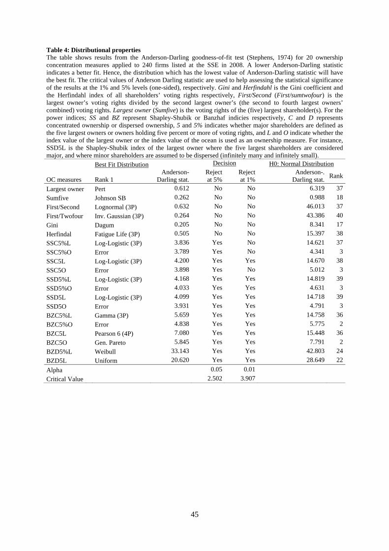
45
Table 4: Distributional properties The table shows results from the Anderson-Darling goodness-of-fit test (Stephens, 1974) for 20 ownership concentration measures applied to 240 firms listed at the SSE in 2008. A lower Anderson-Darling statistic indicates a better fit. Hence, the distribution which has the lowest value of Anderson-Darling statistic will have the best fit. The critical values of Anderson Darling statistic are used to help assessing the statistical significance of the results at the 1% and 5% levels (one-sided), respectively. Gini and Herfindahl is the Gini coefficient and the Herfindahl index of all shareholders’ voting rights respectively, First/Second (First/sumtwofour) is the largest owner’s voting rights divided by the second largest owner’s (the second to fourth largest owners’ combined) voting rights. Largest owner (Sumfive) is the voting rights of the (five) largest shareholder(s). For the power indices; SS and BZ represent Shapley-Shubik or Banzhaf indicies respectively, C and D represents concentrated ownership or dispersed ownership, 5 and 5% indicates whether major shareholders are defined as the five largest owners or owners holding five percent or more of voting rights, and L and O indicate whether the index value of the largest owner or the index value of the ocean is used as an ownership measure. For instance, SSD5L is the Shapley-Shubik index of the largest owner where the five largest shareholders are considered major, and where minor shareholders are assumed to be dispersed (infinitely many and infinitely small). Best Fit Distribution Decision H0: Normal Distribution
OC measures Rank 1 Anderson-
Darling stat.Reject at 5%
Reject at 1%
Anderson-.Darling stat.
Rank
Largest owner Pert 0.612 No No 6.319 37
Sumfive Johnson SB 0.262 No No 0.988 18
First/Second Lognormal (3P) 0.632 No No 46.013 37
First/Twofour Inv. Gaussian (3P) 0.264 No No 43.386 40
Gini Dagum 0.205 No No 8.341 17
Herfindal Fatigue Life (3P) 0.505 No No 15.397 38
SSC5%L Log-Logistic (3P) 3.836 Yes No 14.621 37
SSC5%O Error 3.789 Yes No 4.341 3
SSC5L Log-Logistic (3P) 4.200 Yes Yes 14.670 38
SSC5O Error 3.898 Yes No 5.012 3
SSD5%L Log-Logistic (3P) 4.168 Yes Yes 14.819 39
SSD5%O Error 4.033 Yes Yes 4.631 3
SSD5L Log-Logistic (3P) 4.099 Yes Yes 14.718 39
SSD5O Error 3.931 Yes Yes 4.791 3
BZC5%L Gamma (3P) 5.659 Yes Yes 14.758 36
BZC5%O Error 4.838 Yes Yes 5.775 2
BZC5L Pearson 6 (4P) 7.080 Yes Yes 15.448 36
BZC5O Gen. Pareto 5.845 Yes Yes 7.791 2
BZD5%L Weibull 33.143 Yes Yes 42.803 24
BZD5L Uniform 20.620 Yes Yes 28.649 22
Alpha 0.05 0.01
Critical Value 2.502 3.907
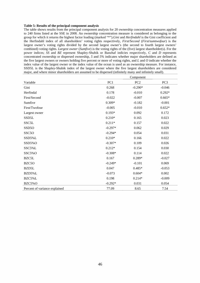
46
Table 5: Results of the principal component analysis The table shows results from the principal component analysis for 20 ownership concentration measures applied to 240 firms listed at the SSE in 2008. An ownership concentration measure is considered as belonging to the group for which it returns the highest factor loading (marked “*”).Gini and Herfindahl is the Gini coefficient and the Herfindahl index of all shareholders’ voting rights respectively, First/Second (First/sumtwofour) is the largest owner’s voting rights divided by the second largest owner’s (the second to fourth largest owners’ combined) voting rights. Largest owner (Sumfive) is the voting rights of the (five) largest shareholder(s). For the power indices; SS and BZ represent Shapley-Shubik or Banzhaf indicies respectively, C and D represents concentrated ownership or dispersed ownership, 5 and 5% indicates whether major shareholders are defined as the five largest owners or owners holding five percent or more of voting rights, and L and O indicate whether the index value of the largest owner or the index value of the ocean is used as an ownership measure. For instance, SSD5L is the Shapley-Shubik index of the largest owner where the five largest shareholders are considered major, and where minor shareholders are assumed to be dispersed (infinitely many and infinitely small).
Component
Variable PC1 PC2 PC3
Gini 0.268 -0.290* -0.046
Herfindal 0.178 -0.010 0.292*
First/Second -0.022 -0.007 0.665*
Sumfive 0.309* -0.182 -0.001
First/Twofour -0.005 -0.010 0.652*
Largest owner 0.193* 0.092 0.172
SSD5L 0.210* 0.165 0.023
SSC5L 0.211* 0.157 0.022
SSD5O -0.297* 0.062 0.029
SSC5O -0.294* 0.054 0.031
SSD5%L 0.210* 0.166 0.022
SSD5%O -0.307* 0.109 0.026
SSC5%L 0.212* 0.154 0.030
SSC5%O -0.308* 0.114 0.022
BZC5L 0.167 0.289* -0.027
BZC5O -0.249* -0.101 0.069
BZD5L 0.047 0.485* -0.053
BZD5%L -0.073 0.604* 0.002
BZC5%L 0.198 0.214* -0.009
BZC5%O -0.292* 0.031 0.054
Percent of variance explained 77.09 8.65 7.54

47
Table 6: Estimation results from OLS regressions The table shows the parameter estimates for the ownership concentration measures only (β1) when running 20 different regressions for each of four different model specifications. In models 1 and 2 (3 and 4) the dependent variable is ln MTB (ROA). In each regression a different ownership measure is used. Accordingly, each cell in the table corresponds to a separate regression. Control variables are not tabulated. Gini and Herfindahl is the Gini coefficient and the Herfindahl index of all shareholders’ voting rights respectively, First/Second (First/sumtwofour) is the largest owner’s voting rights divided by the second largest owner’s (the second to fourth largest owners’ combined) voting rights. Largest owner (Sumfive) is the voting rights of the (five) largest shareholder(s). For the power indices; SS and BZ represent Shapley-Shubik or Banzhaf indicies respectively, C and D represents concentrated ownership or dispersed ownership, 5 and 5% indicates whether major shareholders are defined as the five largest owners or owners holding five percent or more of voting rights, and L and O indicate whether the index value of the largest owner or the index value of the ocean is used as an ownership measure. For instance, SSD5L is the Shapley-Shubik index of the largest owner where the five largest shareholders are considered major, and where minor shareholders are assumed to be dispersed (infinitely many and infinitely small). Heteroscedasticity-robust standard errors (White, 1980) are used. Statistically significant parameter estimates at the 1%, 5%, and 10% levels are denoted by ***, **, and * (two-sided), respectively.
ln MTB ROA Model 1 Model 2 Model 3 Model 4
Gini 0.011 0.002 1.387*** 1.242**(0.554) (0.105) (2.736) (2.511)
Herfindahl 0.001 0.002 0.146** 0.091(0.392) (0.667) (2.480) (1.624)
First/Second 0.002 0.004 0.020 -0.002(0.430) (0.896) (0.267) (0.043)
SumFive -0.001 -0.001 0.196*** 0.158**(0.266) (0.232) (2.829) (2.361)
First/Sumtwofour 0.008 0.013 0,088 0.002(0.599) (1.082) (0.403) (0.009)
Largest owner 0.001 0.001 0.129** 0.083(0.251) (0.493) (2.477) (1.607)
SSD5L 0.000 0.000 0.077** 0.049(0.022) (0.262) (2.412) (1.545)
SSC5L -0.000 -0.000 0.081** 0.057*(0.180) (0.041) (2.554) (1.797)
SSD5O 0.001 0.000 -0.147*** -0.117**(0.194) (0.155) (2.914) (2.356)
SSC5O 0.001 0.001 -0.146*** -0.117**(0.275) (0.268) (2.969) (2.412)
SSD5%L 0.000 0.000 0.077** 0.049(0.017) (0.261) (2.413) (1.542)
SSD5%O 0.001 0.000 -0.145*** -0.118***(0.208) (0.159) (3.204) (2.667)
SSC5%L 0.000 0.000 0.080** 0.051(0.007) (0.261) (2.513) (1.607)
SSC5%O 0.001 0.000 -0.145*** -0.117***(0.222) (0.164) (3.286) (2.708)
BZC5L -0.000 0.000 0.052* 0.029(0.036) (0.178) (1.714) (0.940)
BZC5O 0.001 0.000 -0.109** -0.083*(0.231) (0.172) (2.301) (1.774)
BZD5%L 0.000 0.001 0.005 -0.011(0.181) (0.336) (0.140) (0.293)
BZC5%L -0.001 -0.001 -0.054 -0.067*(0.664) (0.485) (1.370) (1.689)
BZC5%L 0.000 0.001 0.071** 0.045(0.074) (0.288) (2.315) (1.470)
BZC5%O 0.000 0.000 -0.134*** -0.109**(0.136) (0.104) (3.122) (2.590)
Industry dummies No Yes No Yes
Observations 184 184 185 185Min Adj r-square 0,021 0,064 0,339 0,402Max Adj r-square 0,023 0,069 0,389 0,441