Overview on Convenient Calculus andDifferential Geometry in Infinite dimensions, with

Applications to Diffeomorphism Groups andShape Spaces, or

Geodesic evolution equations on shape spacesand diffeormorphism groups

A series of 6 lectures; version 4 from June 26, 2014

Peter W. MichorUniversity of Vienna, Austria

ERC School on Geometric Evolution ProblemsCentro De Giorgi, Pisa

June 23-27, 2014Based on collaborations with: M. Bauer, M. Bruveris, P. Harms, D. Mumford

June 26, 2014

I A short introduction to convenient calculus in infinitedimensions.

I Manifolds of mappings (with compact source) anddiffeomorphism groups as convenient manifolds

I A zoo of diffeomorphism groups on Rn

I A diagram of actions of diffeomorphism groupsI Riemannian geometries of spaces of immersions and shape

spaces.I Right invariant Riemannian geometries on Diffeomorphism

groups.I Arnold’s formula for geodesics on Lie groups.I Solving the Hunter-Saxton equation.I Riemannian geometries on spaces of Riemannian metrics and

pulling them back to diffeomorphism groups.I Approximating Euler’s equation of fluid mechanics on the full

diffeomorphism group of Rn.I Robust Infinite Dimensional Riemannian manifolds, Sobolev

Metrics on Diffeomorphism Groups, and the DerivedGeometry of Shape Spaces.

A short introduction to convenientcalculus in infinite dimensions.

Traditional differential calculus works well for finite dimensionalvector spaces and for Banach spaces.Beyond Banach spaces, the main difficulty is that composition oflinear mappings stops to be jointly continuous at the level ofBanach spaces, for any compatible topology.For more general locally convex spaces we sketch here theconvenient approach as explained in [Frolicher-Kriegl 1988] and[Kriegl-Michor 1997].

The c∞-topology

Let E be a locally convex vector space. A curve c : R→ E iscalled smooth or C∞ if all derivatives exist and are continuous. LetC∞(R,E ) be the space of smooth functions. It can be shown thatthe set C∞(R,E ) does not depend on the locally convex topologyof E , only on its associated bornology (system of bounded sets).The final topologies with respect to the following sets of mappingsinto E coincide:

1. C∞(R,E ).

2. The set of all Lipschitz curves (so that

c(t)−c(s)t−s : t 6= s, |t|, |s| ≤ C is bounded in E , for each C ).

3. The set of injections EB → E where B runs through allbounded absolutely convex subsets in E , and where EB is thelinear span of B equipped with the Minkowski functional‖x‖B := infλ > 0 : x ∈ λB.

4. The set of all Mackey-convergent sequences xn → x (thereexists a sequence 0 < λn ∞ with λn(xn − x) bounded).

The c∞-topology. II

This topology is called the c∞-topology on E and we write c∞Efor the resulting topological space.In general (on the space D of test functions for example) it is finerthan the given locally convex topology, it is not a vector spacetopology, since scalar multiplication is no longer jointly continuous.The finest among all locally convex topologies on E which arecoarser than c∞E is the bornologification of the given locallyconvex topology. If E is a Frechet space, then c∞E = E .

Convenient vector spaces

A locally convex vector space E is said to be a convenient vectorspace if one of the following holds (called c∞-completeness):

1. For any c ∈ C∞(R,E ) the (Riemann-) integral∫ 1

0 c(t)dtexists in E .

2. Any Lipschitz curve in E is locally Riemann integrable.

3. A curve c : R→ E is C∞ if and only if λ c is C∞ for allλ ∈ E ∗, where E ∗ is the dual of all cont. lin. funct. on E .

I Equiv., for all λ ∈ E ′, the dual of all bounded lin. functionals.I Equiv., for all λ ∈ V, where V is a subset of E ′ which

recognizes bounded subsets in E .

We call this scalarwise C∞.

4. Any Mackey-Cauchy-sequence (i. e. tnm(xn − xm)→ 0 forsome tnm →∞ in R) converges in E . This is visibly a mildcompleteness requirement.

Convenient vector spaces. II

5. If B is bounded closed absolutely convex, then EB is a Banachspace.

6. If f : R→ E is scalarwise Lipk , then f is Lipk , for k > 1.

7. If f : R→ E is scalarwise C∞ then f is differentiable at 0.

Here a mapping f : R→ E is called Lipk if all derivatives up toorder k exist and are Lipschitz, locally on R. That f is scalarwiseC∞ means λ f is C∞ for all continuous (equiv., bounded) linearfunctionals on E .

Smooth mappings

Let E , and F be convenient vector spaces, and let U ⊂ E bec∞-open. A mapping f : U → F is called smooth or C∞, iff c ∈ C∞(R,F ) for all c ∈ C∞(R,U).If E is a Frechet space, then this notion coincides with all otherreasonable notions of C∞-mappings. Beyond Frechet mappings, asa rule, there are more smooth mappings in the convenient settingthan in other settings, e.g., C∞c .

Main properties of smooth calculus

1. For maps on Frechet spaces this coincides with all otherreasonable definitions. On R2 this is non-trivial [Boman,1967].

2. Multilinear mappings are smooth iff they are bounded.

3. If E ⊇ Uf−−→ F is smooth then the derivative

df : U × E → F is smooth, and also df : U → L(E ,F ) issmooth where L(E ,F ) denotes the space of all bounded linearmappings with the topology of uniform convergence onbounded subsets.

4. The chain rule holds.

5. The space C∞(U,F ) is again a convenient vector space wherethe structure is given by the obvious injection

C∞(U,F )C∞(c,`)−−−−−−→

∏c∈C∞(R,U),`∈F∗

C∞(R,R), f 7→ (` f c)c,`,

where C∞(R,R) carries the topology of compact convergencein each derivative separately.

Main properties of smooth calculus, II

6. The exponential law holds: For c∞-open V ⊂ F ,

C∞(U,C∞(V ,G )) ∼= C∞(U × V ,G )

is a linear diffeomorphism of convenient vector spaces.Note that this is the main assumption of variational calculus.Here it is a theorem.

7. A linear mapping f : E → C∞(V ,G ) is smooth (by (2)equivalent to bounded) if and only if

Ef−−→ C∞(V ,G )

evv−−−→ G is smooth for each v ∈ V .

(Smooth uniform boundedness theorem,see [KM97], theorem 5.26).

Main properties of smooth calculus, III

8. The following canonical mappings are smooth.

ev : C∞(E ,F )× E → F , ev(f , x) = f (x)

ins : E → C∞(F ,E × F ), ins(x)(y) = (x , y)

( )∧ : C∞(E ,C∞(F ,G ))→ C∞(E × F ,G )

( )∨ : C∞(E × F ,G )→ C∞(E ,C∞(F ,G ))

comp : C∞(F ,G )× C∞(E ,F )→ C∞(E ,G )

C∞( , ) : C∞(F ,F1)× C∞(E1,E )→→ C∞(C∞(E ,F ),C∞(E1,F1))

(f , g) 7→ (h 7→ f h g)∏:∏

C∞(Ei ,Fi )→ C∞(∏

Ei ,∏

Fi )

This ends our review of the standard results of convenient calculus.Convenient calculus (having properties 6 and 7) exists also for:

I Real analytic mappings [Kriegl,M,1990]

I Holomorphic mappings [Kriegl,Nel,1985] (notion of[Fantappie, 1930-33])

I Many classes of Denjoy Carleman ultradifferentible functions,both of Beurling type and of Roumieu-type[Kriegl,M,Rainer, 2009, 2011, 2013]

I With some adaptations, Lipk [Frolicher-Kriegl, 1988].

I With more adaptations, even C k,α (k-th derivativeHolder-contin. with index α) [Faure,Frolicher 1989], [Faure,These Geneve, 1991]

Manifolds of mappings (with compact source) anddiffeomorphism groups as convenient manifolds.

Let M be a compact (for simplicity’s sake) fin. dim. manifold andN a manifold. We use an auxiliary Riemann metric g on N. Then

0N_

zero section

N _

diagonal

%%TN V N? _

openoo (πN ,expg )

∼=// V N×N

open// N × N

C∞(M,N), the space of smooth mappings M → N, has thefollowing manifold structure. Chart, centered at f ∈ C∞(M,N), is:

C∞(M,N) ⊃ Uf = g : (f , g)(M) ⊂ V N×N uf−−−→ Uf ⊂ Γ(f ∗TN)

uf (g) = (πN , expg )−1 (f , g), uf (g)(x) = (expgf (x))−1(g(x))

(uf )−1(s) = expgf s, (uf )−1(s)(x) = expgf (x)(s(x))

Manifolds of mappings II

Lemma: C∞(R, Γ(M; f ∗TN)) = Γ(R×M; pr2∗ f ∗TN)

By Cartesian Closedness (after trivializing the bundle f ∗TN).Lemma: Chart changes are smooth (C∞)Uf1 3 s 7→ (πN , expg ) s 7→ (πN , expg )−1 (f2, expg

f1s)

since they map smooth curves to smooth curves.Lemma: C∞(R,C∞(M,N)) ∼= C∞(R×M,N).By the first lemma.Lemma: Composition C∞(P,M)× C∞(M,N)→ C∞(P,N),(f , g) 7→ g f , is smooth, since it maps smooth curves to smoothcurvesCorollary (of the chart structure):

TC∞(M,N) = C∞(M,TN)C∞(M,πN)−−−−−−−−→ C∞(M,N).

Regular Lie groups

We consider a smooth Lie group G with Lie algebra g = TeGmodelled on convenient vector spaces. The notion of a regular Liegroup is originally due to Omori et al. for Frechet Lie groups, wasweakened and made more transparent by Milnor, and then carriedover to convenient Lie groups; see [KM97], 38.4.A Lie group G is called regular if the following holds:

I For each smooth curve X ∈ C∞(R, g) there exists a curveg ∈ C∞(R,G ) whose right logarithmic derivative is X , i.e.,

g(0) = e

∂tg(t) = Te(µg(t))X (t) = X (t).g(t)

The curve g is uniquely determined by its initial value g(0), ifit exists.

I Put evolrG (X ) = g(1) where g is the unique solution requiredabove. Then evolrG : C∞(R, g)→ G is required to be C∞

also. We have EvolXt := g(t) = evolG (tX ).

Diffeomorphism group of compact M

Theorem: For each compact manifold M, the diffeomorphismgroup is a regular Lie group.Proof: Diff(M)

open−−−−→ C∞(M,M). Composition is smooth by

restriction. Inversion is smooth: If t 7→ f (t, ) is a smooth curvein Diff(M), then f (t, )−1 satisfies the implicit equationf (t, f (t, )−1(x)) = x , so by the finite dimensional implicitfunction theorem, (t, x) 7→ f (t, )−1(x) is smooth. So inversionmaps smooth curves to smooth curves, and is smooth.Let X (t, x) be a time dependent vector field on M (inC∞(R,X(M))). Then Fl∂t×Xs (t, x) = (t + s,EvolX (t, x)) satisfiesthe ODE ∂t Evol(t, x) = X (t,Evol(t, x)). IfX (s, t, x) ∈ C∞(R2,X(M)) is a smooth curve of smooth curves inX(M), then obviously the solution of the ODE depends smoothlyalso on the further variable s, thus evol maps smooth curves oftime dependant vector fields to smooth curves of diffeomorphism.QED.

The principal bundle of embeddings

For finite dimensional manifolds M, N with M compact,Emb(M,N), the space of embeddings of M into N, is open inC∞(M,N), so it is a smooth manifold. Diff(M) acts freely andsmoothly from the right on Emb(M,N).Theorem: Emb(M,N)→ Emb(M,N)/Diff(M) is a principal fiberbundle with structure group Diff(M).Proof: Auxiliary Riem. metric g on N. Given f ∈ Emb(M,N),view f (M) as submanifold of N. TN|f (M) = Nor(f (M))⊕ Tf (M).

Nor(f (M)) :expg

−−−−→∼= Wf (M)

pf (M)−−−−→ f (M) tubular nbhd of f (M).

If g : M → N is C 1-near to f , thenϕ(g) := f −1 pf (M) g ∈ Diff(M) andg ϕ(g)−1 ∈ Γ(f ∗Wf (M)) ⊂ Γ(f ∗Nor(f (M))).This is the required local splitting. QED

The orbifold bundle of immersions

Imm(M,N), the space of immersions M → N, is open inC∞(M,N), and is thus a smooth manifold. The regular Lie groupDiff(M) acts smoothly from the right, but no longer freely.Theorem: [Cervera,Mascaro,M,1991] For an immersionf : M → N, the isotropy groupDiff(M)f = ϕ ∈ Diff(M) : f φ = f is always a finite group,

acting freely on M; so Mp−−→ M/Diff(M)f is a convering of

manifold and f factors to f = f p.Thus Imm(M,N)→ Imm(M,N)/Diff (M) is a projection onto anhonest infinite dimensional orbifold.

A Zoo of diffeomorphism groups on Rn

Theorem. The following groups of diffeomorphisms on Rn areregular Lie groups:

I DiffB(Rn), the group of all diffeomorphisms which differ fromthe identity by a function which is bounded together with allderivatives separately.

I DiffH∞(Rn), the group of all diffeomorphisms which differfrom the identity by a function in the intersection H∞ of allSobolev spaces Hk for k ∈ N≥0.

I DiffS(Rn), the group of all diffeomorphisms which fall rapidlyto the identity.

I Diffc(Rn) of all diffeomorphisms which differ from the identityonly on a compact subset. (well known since 1980)

[M,Mumford,2013], partly [B.Walter,2012]; for Denjoy-Carleman ultradifferentiable diffeomorphisms [Kriegl, M,Rainer 2014].In particular, DiffH∞ (Rn) is essential if one wants to prove that the geodesic equation of a right Riemannianinvariant metric is well-posed with the use of Sobolov space techniques.

A Zoo of diffeomorphism groups on Rn

We need more on convenient calculus.[FK88], theorem 4.1.19.Theorem. Let c : R→ E be a curve in a convenient vector spaceE . Let V ⊂ E ′ be a subset of bounded linear functionals such thatthe bornology of E has a basis of σ(E ,V)-closed sets. Then thefollowing are equivalent:

1. c is smooth

2. There exist locally bounded curves ck : R→ E such that ` cis smooth R→ R with (` c)(k) = ` ck , for each ` ∈ V.

If E is reflexive, then for any point separating subset V ⊂ E ′ thebornology of E has a basis of σ(E ,V)-closed subsets, by [FK88],4.1.23.

A Zoo of diffeomorphism groups on Rn

Faa di Bruno formula.Let g ∈ C∞(Rn,Rk) and let f ∈ C∞(Rk ,Rl). Then the p-thdeivative of f g looks as follows where symp denotessymmetrization of a p-linear mapping:

dp(f g)(x)

p!=

= symp

( p∑j=1

∑α∈Nj

>0α1+···+αj=p

d j f (g(x))

j!

(dα1g(x)

α1!, . . . ,

dαj g(x)

αj !

))

The one dimensional version is due to [Faa di Bruno 1855], theonly beatified mathematician.

Groups of smooth diffeomorphisms in the zoo

If we consider the group of all orientation preservingdiffeomorphisms Diff(Rn) of Rn, it is not an open subset ofC∞(Rn,Rn) with the compact C∞-topology. So it is not a smoothmanifold in the usual sense, but we may consider it as a Lie groupin the cartesian closed category of Frolicher spaces, see [KM97],section 23, with the structure induced by the injectionf 7→ (f , f −1) ∈ C∞(Rn,Rn)× C∞(Rn,R).We shall now describe regular Lie groups in Diff(Rn) which aregiven by diffeomorphisms of the form f = IdR +g where g is insome specific convenient vector spaces of bounded functions inC∞(Rn,Rn). Now we discuss these spaces on Rn, we describe thesmooth curves in them, and we describe the corresponding groups.

The group DiffB(Rn) in the zoo

The space B(Rn) (called DL∞(Rn) by [L.Schwartz 1966]) consistsof all smooth functions which have all derivatives (separately)bounded. It is a Frechet space. By [Vogt 1983], the space B(Rn)is linearly isomorphic to `∞⊗ s for any completed tensor-productbetween the projective one and the injective one, where s is thenuclear Frechet space of rapidly decreasing real sequences. ThusB(Rn) is not reflexive, not nuclear, not smoothly paracompact.The space C∞(R,B(Rn)) of smooth curves in B(Rn) consists ofall functions c ∈ C∞(Rn+1,R) satisfying the following property:

• For all k ∈ N≥0, α ∈ Nn≥0 and each t ∈ R the expression

∂kt ∂αx c(t, x) is uniformly bounded in x ∈ Rn, locally in t.

To see this use thm FK for the set evx : x ∈ R of point

evaluations in B(Rn). Here ∂αx = ∂|α|

∂xα and ck(t) = ∂kt f (t, ).Diff+

B (Rn) =

f = Id +g : g ∈ B(Rn)n, det(In + dg) ≥ ε > 0

denotes the corresponding group, see below.

The group DiffH∞(Rn) in the zoo

The space H∞(Rn) =⋂

k≥1 Hk(Rn) is the intersection of allSobolev spaces which is a reflexive Frechet space. It is calledDL2(Rn) in [L.Schwartz 1966]. By [Vogt 1983], the space H∞(Rn)is linearly isomorphic to `2⊗ s. Thus it is not nuclear, notSchwartz, not Montel, but still smoothly paracompact.The space C∞(R,H∞(Rn)) of smooth curves in H∞(Rn) consistsof all functions c ∈ C∞(Rn+1,R) satisfying the following property:

• For all k ∈ N≥0, α ∈ Nn≥0 the expression ‖∂kt ∂αx f (t, )‖L2(Rn)

is locally bounded near each t ∈ R.

The proof is literally the same as for B(Rn), noting that the pointevaluations are continuous on each Sobolev space Hk with k > n

2 .Diff+

H∞(R) =

f = Id +g : g ∈ H∞(R), det(In + dg) > 0

denotesthe correponding group.

The group DiffS(Rn) in the zoo

The algebra S(Rn) of rapidly decreasing functions is a reflexivenuclear Frechet space.The space C∞(R,S(Rn)) of smooth curves in S(Rn) consists ofall functions c ∈ C∞(Rn+1,R) satisfying the following property:

• For all k ,m ∈ N≥0 and α ∈ Nn≥0, the expression

(1 + |x |2)m∂kt ∂αx c(t, x) is uniformly bounded in x ∈ Rn,

locally uniformly bounded in t ∈ R.

Diff+S (Rn) =

f = Id +g : g ∈ S(Rn)n, det(In + dg) > 0

is the

correponding group.

The group Diffc(Rn) in the zoo

The algebra C∞c (Rn) of all smooth functions with compactsupport is a nuclear (LF)-space.The space C∞(R,C∞c (Rn)) of smooth curves in C∞c (Rn) consistsof all functions f ∈ C∞(Rn+1,R) satisfying the following property:

• For each compact interval [a, b] in R there exists a compactsubset K ⊂ Rn such that f (t, x) = 0 for(t, x) ∈ [a, b]× (Rn \ K ).

Diffc(Rn) =

f = Id +g : g ∈ C∞c (Rn)n, det(In + dg) > 0

is thecorreponding group.

Ideal properties of function spaces in the zoo

The function spaces are boundedly mapped into each other asfollows:

C∞c (Rn) // S(Rn) // H∞(Rn) // B(Rn)

and each space is a bounded locally convex algebra and a boundedB(Rn)-module. Thus each space is an ideal in each larger space.

Main theorem in the Zoo

Theorem. The sets of diffeomorphisms Diffc(Rn), DiffS(Rn),DiffH∞(Rn), and DiffB(Rn) are all smooth regular Lie groups. Wehave the following smooth injective group homomorphisms

Diffc(Rn) // DiffS(Rn) // DiffH∞(Rn) // DiffB(Rn) .

Each group is a normal subgroup in any other in which it iscontained, in particular in DiffB(Rn).Corollary. DiffB(Rn) acts on Γc , ΓS and ΓH∞ of any tensorbundleover Rn by pullback. The infinitesimal action of the Lie algebraXB(Rn) on these spaces by the Lie derivative thus maps each ofthese spaces into itself. A fortiori, DiffH∞(Rn) acts on ΓS of anytensor bundle by pullback.

Proof of the main zoo theorem

Let A denote any of B, H∞, S, or c, and let A(Rn) denote thecorresponding function space. Let f (x) = x + g(x) for g ∈ A(Rn)n

with det(In + dg) > 0 and for x ∈ Rn.Each such f is a diffeomorphism. By the inverse function theoremf is a locally a diffeomorphism everywhere. Thus the image of f isopen in Rn. We claim that it is also closed. So let xi ∈ Rn withf (xi ) = xi + g(xi )→ y0 in Rn. Then f (xi ) is a bounded sequence.Since g ∈ A(Rn) ⊂ B(Rn), the xi also form a bounded sequence,thus contain a convergent subsequence. Without loss let xi → x0

in Rn. Then f (xi )→ f (x0) = y0. Thus f is surjective. This alsoshows that f is a proper mapping (i.e., compact sets have compactinverse images under f ). A proper surjective submersion is theprojection of a smooth fiber bundle. In our case here f has discretefibers, so f is a covering mapping and a diffeomorphism since Rn issimply connected.

DiffA(Rn)0 is closed under composition.

((Id +f ) (Id +g))(x) = x + g(x) + f (x + g(x))

We have to check that x 7→ f (x + g(x)) is in A(Rn) iff , g ∈ A(Rn)n. For A = B this follows by the Faa di Brunoformula. For A = S or S1 we need furthermore:

(∂αx f )(x + g(x)) = O(

1(1+|x+g(x)|2)k

)= O

(1

(1+|x |2)k

)which holds

since 1+|x |21+|x+g(x)|2 is globally bounded.

For A = H∞ we also need that∫Rn

|(∂αx f )(x + g(x))|2 dx = (3)∫Rn

|(∂αf )(y)|2 dy| det(In+dg)((Id +g)−1(y))| ≤ C (g)

∫Rn

|(∂αf )(y)|2dy ;

this holds since the denominator is globally bounded away from 0since g and dg vanish at ∞ by the lemma of Riemann-Lebesque.The case A(Rn) = C∞c (Rn) or C∞c,1(Rn) is easy and well known.

Multiplication is smooth on DiffA(Rn).

Suppose that the curves t 7→ Id +f (t, ) and t 7→ Id +g(t, ) arein C∞(R,DiffA(Rn)) which means that the functionsf , g ∈ C∞(Rn+1,Rn) satisfy condition A.We have to check that f (t, x + g(t, x)) also satisfies condition A.For this we reread the proof that composition preserves DiffA(Rn)and pay attention to the further parameter t.

The inverse (Id +g)−1 is again an element in DiffA(Rn)

For g ∈ A(Rn)n we write (Id +g)−1 = Id +f .We have to check that f ∈ A(Rn)n.

(Id +f ) (Id +g) = Id =⇒ x + g(x) + f (x + g(x)) = x

=⇒ x 7→ f (x + g(x)) = −g(x) is in A(Rn)n.

First the case A = B. We know already that Id +g is adiffeomorphism. By definition, we have det(In + dg(x)) ≥ ε > 0for some ε. This implies that

‖(In + dg(x))−1‖L(Rn,Rn) is globally bounded,

using that ‖A−1‖ ≤ ‖A‖n−1

| det(A)| for any linear A : Rn → Rn. Moreover,

(In+df (x+g(x)))(In+dg(x)) = In =⇒ det(In+df (x+g(x))) =

= det(In + dg(x))−1 ≥ ‖In + dg(x)‖−n ≥ η > 0 for all x .

For higher derivatives we write the Faa di Bruno formula as:

dp(f (Id +g))(x)

p!= symp

( p∑j=1

∑α∈Nj

>0α1+···+αj=p

d j f (x + g(x))

j!

(dα1(Id +g)(x)

α1!, . . . ,

dαj (Id +g)(x)

αj !

))=

dpf (x + g(x))

p!

(Id +dg(x), . . . , Id +dg(x)

)(top extra)

+ symp−1

( p−1∑j=1

∑α∈Nj

>0α1+···+αj=p(hα1 ,...,hαj )

d j f (x + g(x))

j!

(dα1hα1(x)

α1!, . . . ,

dαj hαj (x)

αj !

))

where hαi (x) is g(x) for αi > 1 (there is always such an i), andwhere hαi (x) = x or g(x) if αi = 1.

Now we argue as follows:The left hand side is globally bounded. We already know thatId +dg(x) : Rn → Rn is invertible with ‖(In + dg(x))−1‖L(Rn,Rn)

globally bounded.Thus we can conclude by induction on p that dpf (x + g(x)) isbounded uniformly in x , thus also uniformy in y = x + g(x) ∈ R.For general A we note that the left hand side is in A. Since wealready know that f ∈ B, and since A is a B-module, the last termis in A. Thus also the first term is in A, and any summand therecontaining just one dg(x) is in A, so the unique summanddpf (x , g(x)) is also in A. Thus inversion maps DiffA(R) into itself.

Inversion is smooth on DiffA(Rn).

We retrace the proof that inversion preserves DiffA assuming thatg(t, x) satisfies condition A.We see again that f (t, x + g(t, x)) = −g(t, x) satisfies conditionA as a function of t, x , and we claim that f then does the same.We reread the proof paying attention to the parameter t and seethat condition A is satisfied.

DiffA(Rn) is a regular Lie group

So let t 7→ X (t, ) be a smooth curve in the Lie algebraXA(Rn) = A(Rn)n, i.e., X satisfies condition A.The evolution of this time dependent vector field is the functiongiven by the ODE

Evol(X )(t, x) = x + f (t, x),∂t(x + f (t, x)) = ft(t, x) = X (t, x + f (t, x)),

f (0, x) = 0.(7)

We have to showfirst that f (t, ) ∈ A(Rn)n for each t ∈ R,second that it is smooth in t with values in A(Rn)n, andthird that X 7→ f is also smooth.

For 0 ≤ t ≤ C we consider

|f (t, x)| ≤∫ t

0|ft(s, x)|ds =

∫ t

0|X (s, x + f (s, x))| ds. (8)

Since A ⊆ B, the vector field X (t, y) is uniformly bounded iny ∈ Rn, locally in t. So the same is true for f (t, x) by (7).

Next consider

∂tdx f (t, x) = dx(X (t, xf (t, x))) (9)

= (dxX )(t, x + f (t, x)) + (dxX )(t, x + f (t, x)).dx f (t, x)

‖dx f (t, x)‖ ≤∫ t

0‖(dxX )(s, x + f (s, x))‖ds

+

∫ t

0‖(dxX )(s, x + f (s, x))‖.‖dx f (s, x)‖ds

=: α(t, x) +

∫ t

0β(s, x).‖dx f (s, x)‖ds

By the Bellman-Gronwall inequality,

‖dx f (t, x)‖ ≤ α(t, x) +

∫ t

0α(s, x).β(s, x).e

∫ ts β(σ,x) dσ ds,

which is globally bounded in x , locally in t.

For higher derivatives in x (where p > 1) we use Faa di Bruno as

∂tdpx f (t, x) = dp

x (X (t, x + f (t, x))) = symp

( p∑j=1

∑α∈Nj

>0α1+···+αj=p

(d jxX )(t, x + f (t, x))

j!

(dα1x (x + f (t, x))

α1!, . . . ,

dαjx (x + f (t, x))

αj !

))= (dxX )(t, x + f (t, x))

(dpx f (t, x)

)+ (bottom extra)

+ symp

( p∑j=2

∑α∈Nj

>0α1+···+αj=p

(d jxX )(t, x + f (t, x))

j!

(dα1x (x + f (t, x))

α1!, . . . ,

dαjx (x + f (t, x))

αj !

))

We can assume recursively that d jx f (t, x) is globally bounded in x ,

locally in t, for j < p. Then we have reproduced the situation of(9) (with values in the space of symmetric p-linear mappings(Rn)p → Rn) and we can repeat the argument above involving theBellman-Gronwall inequality to conclude that dp

x f (t, x) is globallybounded in x , locally in t.To conclude the same for ∂mt dp

x f (t, x) we just repeat the lastarguments for ∂mt f (t, x). So we have now proved thatf ∈ C∞(R,XB(Rn)).To prove that C∞(R,XB(Rn)) 3 X 7→ Evol(X )(1, ) ∈ DiffB(Rn)is smooth, we consider a smooth curve X in C∞(R,XB(Rn)); thusX (t1, t2, x) is smooth on R2 × Rn, globally bounded in x in eachderivative separately, locally in t = (t1, t2) in each derivative. Or,we assume that t is 2-dimensional in the argument above. Butthen it suffices to show that (t1, t2) 7→ X (t1, t2, ) ∈ XB(Rn) issmooth along smooth curves in R2, and we are again in thesituation we have just treated.Thus DiffB(Rn) is a regular Lie group.

If A = S, we already know that f (s, x) is globally bounded in x ,locally in t. Thus may insertX (s, x + f (s, x)) = O( 1

(1+|x+f (s,x)|2)k) = O( 1

(1+|x |2)k) into (8) and

can conclude that f (t, x) = O( 1(1+|x |2)k

) globally in x , locally in t,

for each k .Using this argument, we can repeat the proof for the case A = Bfrom above.Thus DiffS(Rn) is a regular Lie group.

If A = H∞ we first consider the differential of (8),

‖dx f (s, x)‖ =∥∥∥∫ t

0dx(X (s, ))(x + f (s, x)).(In + df (s, )(x)) ds

∥∥∥≤∫ t

0

∥∥dx(X (s, ))(x + f (s, x))∥∥.C , ds (10)

since dx f (s, x) is globally bounded in x , locally in s, by the caseA = B. The same holds for f (s, x). Moreover, X (s, ) vanishesnear infinity by the lemma of Riemann-Lebesque, so that the sameholds for f (s, ) by (10).

Now we consider∫Rn

‖(dpx f )(t, x)‖2 dx =

∫Rn

∥∥∥∫ t

0dpx

(X (s, Id +f (s, ))

)(x) ds

∥∥∥2dx .

We apply Faa di Bruno in the form (top extra) to the integrand,remember that we already know that each dαi (Id +f (s, ))(x) isglobally bounded, locally in s, thus the last term is

≤∫Rn

(∫ t

0

p∑j=1

‖(d jxX )(s, x + f (s, x))‖.Cj ds

)2dx

=

∫Rn

(∫ t

0

p∑j=1

‖(d jxX )(s, y)‖.Cj ds

)2dy

| det(In+df (s, ))((In+f (s, ))−1(y)|

which is finite since X (s, ) ∈ H∞ and since the determinand inthe denominator is bounded away from zero – we just checked thatdx f (s, ) vanishes at infinity. We repeat this for ∂mt dp

x f (t, x).This shows that Evol(X )(t, ) ∈ DiffH∞(Rn) for each t.Choosing t two-dimensional (as in the case A = B) we canconclude that DiffH∞(Rn) is a regular Lie group.

DiffS(Rn) is a normal subgroup of DiffB(Rn).

So let g ∈ B(Rn)n with det(In + dg(x)) ≥ ε > 0 for all x , ands ∈ S(Rn)n with det(In + ds(x)) > 0 for all x . We consider

(Id + g)−1(x) = x + f (x) for f ∈ B(Rn)n

⇐⇒ f (x + g(x)) = −g(x)

((Id + g)−1 (Id +s) (Id +g))(x) = ((Id +f ) (Id +s) (Id +g)

)(x) =

= x + g(x) + s(x + g(x)) + f(x + g(x) + s(x + g(x))

)= x + s(x + g(x))− f (x + g(x)) + f

(x + g(x) + s(x + g(x))

).

Since g(x) is globally bounded we gets(x + g(x)) = O((1 + |x + g(x)|−k) = O((1 + |x |)−k) for each k .For dp

x (s (Id +g))(x) this follows from Faa di Bruno in the formof (top extra).

Moreover we have

f(x + g(x) + s(x + g(x))

)− f (x + g(x)) =

=

∫ 1

0df(x + g(x) + ts(x + g(x))

)(s(x + g(x))) dt

which is in S(Rn)n as a function of x since df is in B ands(x + g(x)) is in S.

DiffH∞(Rn) is a normal subgroup of DiffB(Rn).

We redo the last proof under the assumption that s ∈ H∞(Rn)n.By the argument in (3) we see that s(x + g(x)) is in H∞ as afunction of x .The rest is as above.This finishes the proof of the main theorem.

A diagram of actions of diffeomorphism groups.

Diff(M)r-acts //

r-acts

%%Diff(M,µ)

Imm(M,N)

needs gxx Diff(M) &&

DiffA(N)

r-acts

l-acts

(LDDMM)oo

l-acts

(LDDMM)xxMet(M)

Diff(M) %% %%

Bi (M,N)

needs gxxVol1+(M) Met(M)

Diff(M) MetA(N)

M compact ,N pssibly non-compact manifold

Met(N) = Γ(S2+T∗N) space of all Riemann metrics on N

g one Riemann metric on N

Diff(M) Lie group of all diffeos on compact mf M

DiffA(N), A ∈ H∞,S, c Lie group of diffeos of decay A to IdN

Imm(M,N) mf of all immersions M → N

Bi (M,N) = Imm/Diff(M) shape space

Vol1+(M) ⊂ Γ(vol(M)) space of positive smooth probability densities

Diff(S1)r-acts //

r-acts

%%r-acts

Imm(S1,R2)

needs gxx Diff(S1) ''

DiffA(R2)

r-acts

l-acts

(LDDMM)oo

l-acts

(LDDMM)xxVol+(S1)

Met(S1)

Diff(S1)

&& &&

Bi (S1,R2)

needs gxxVol+(S1)Diff(S1)

∫fdθ

=// R>0

Met(S1)Diff(S1)∫ √

gdθ

=oo Met(R2)

Diff(S1) Lie group of all diffeos on compact mf S1

DiffA(R2), A ∈ B,H∞,S, c Lie group of diffeos of decay A to IdR2

Imm(S1,R2) mf of all immersions S1 → R2

Bi (S1,R2) = Imm/Diff(S1) shape space

Vol+(S1) =f dθ : f ∈ C∞(S1

,R>0)

space of positive smooth probability densities

Met(S1) =g dθ2 : g ∈ C∞(S1

,R>0)

space of metrics on S1

The manifold of immersions

Let M be either S1 or [0, 2π].

Imm(M,R2) := c ∈ C∞(M,R2) : c ′(θ) 6= 0 ⊂ C∞(M,R2).

The tangent space of Imm(M,R2) at a curve c is the set of allvector fields along c :

Tc Imm(M,R2) =

h :

TR2

π

Mc //

h

==

R2

∼= h ∈ C∞(M,R2)

Some Notation:

v(θ) =c ′(θ)

|c ′(θ)|, n(θ) = iv(θ), ds = |c ′(θ)|dθ, Ds =

1

|c ′(θ)|∂θ

Diff(S1)r-acts //

r-acts $$

Imm(S1,R2)

needs gxx Diff(S1) ''

Diffc(R2)l-acts

(LDDMM)oo

l-acts

(LDDMM)xxMet(S1) Bi (S1,R2)

Emb(S1,R2)

// Imm(S1,R2)

Emb(S1,R2)/Diff(S1)

// Imm(S1,R2)/Diff(S1)

B(S1,R2) Bi (S1,R2)

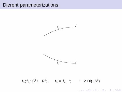
Different parameterizations

f1//

f2 //

f1, f2 : S1 → R2, f1 = f2 ϕ, ϕ ∈ Diff(S1)

Inducing a metric on shape space

Imm(M,N)

π

Bi := Imm(M,N)/Diff(M)

Every Diff(M)-invariant metric ”above“ induces a unique metric”below“ such that π is a Riemannian submersion.

Inner versus Outer

The vertical and horizontal bundle

I T Imm = Vert⊕

Hor.

I The vertical bundle is

Vert := ker Tπ ⊂ T Imm .

I The horizontal bundle is

Hor := (ker Tπ)⊥,G ⊂ T Imm .

It might not be a complement - sometimes one has to go tothe completion of (Tf Imm,Gf ) in order to get a complement.

The vertical and horizontal bundle

Definition of a Riemannian metric

Imm(M,N)

π

Bi (M,N)

1. Define a Diff(M)-invariant metric Gon Imm.

2. If the horizontal space is acomplement, then Tπ restricted tothe horizontal space yields anisomorphism

(ker Tf π)⊥,G ∼= Tπ(f )Bi .

Otherwise one has to induce thequotient metric, or use thecompletion.

3. This gives a metric on Bi such thatπ : Imm→ Bi is a Riemanniansubmersion.

Riemannian submersions

Imm(M,N)

π

Bi := Imm(M,N)/Diff(M)

I Horizontal geodesics on Imm(M,N) project down to geodesicsin shape space.

I O’Neill’s formula connects sectional curvature on Imm(M,N)and on Bi .

[Micheli, M, Mumford, Izvestija 2013]

L2 metric

G 0c (h, k) =

∫M〈h(θ), k(θ)〉ds.

Problem: The induced geodesic distance vanishes.

Diff(S1)r-acts //

r-acts $$

Imm(S1,R2)

needs gxx Diff(S1) ''

Diffc(R2)l-acts

(LDDMM)oo

l-acts

(LDDMM)xxMet(S1) Bi (S1,R2)

Movies about vanishing: Diff(S1) Imm(S1,R2)

[MichorMumford2005a,2005b], [BauerBruverisHarmsMichor2011,2012]

The simplest (L2-) metric on Imm(S1,R2)

G 0c (h, k) =

∫S1

〈h, k〉ds =

∫S1

〈h, k〉|cθ| dθ

Geodesic equation

ctt = − 1

2|cθ|∂θ

( |ct |2 cθ|cθ|

)− 1

|cθ|2〈ctθ, cθ〉ct .

A relative of Burger’s equation.Conserved momenta for G 0 along any geodesic t 7→ c( , t):

〈v , ct〉|cθ|2 ∈ X(S1) reparam. mom.∫S1

ctds ∈ R2 linear moment.∫S1

〈Jc , ct〉ds ∈ R angular moment.

Horizontal Geodesics for G 0 on Bi (S1,R2)

〈ct , cθ〉 = 0 and ct = an = aJ cθ|cθ| for a ∈ C∞(S1,R). We use

functions a, s = |cθ|, and κ, only holonomic derivatives:

st = −aκs, at = 12κa2,

κt = aκ2 +1

s

(aθs

)θ

= aκ2 +aθθs2− aθsθ

s3.

We may assume s|t=0 ≡ 1. Let v(θ) = a(0, θ), the initial value fora. Thensts = −aκ = −2at

a , so log(sa2)t = 0, thuss(t, θ)a(t, θ)2 = s(0, θ)a(0, θ)2 = v(θ)2,

a conserved quantity along the geodesic. We substitute s = v2

a2 andκ = 2 at

a2 to get

att − 4a2t

a− a6aθθ

2v 4+

a6aθvθv 5

−a5a2

θ

v 4= 0,

a(0, θ) = v(θ),

a nonlinear hyperbolic second order equation. Note that whereverv = 0 then also a = 0 for all t. So substitute a = vb. Theoutcome is

(b−3)tt = −v 2

2(b3)θθ − 2vvθ(b3)θ −

3vvθθ2

b3,

b(0, θ) = 1.

This is the codimension 1 version whereBurgers’ equation is the codimension 0 version.

Weak Riem. metrics on Emb(M ,N) ⊂ Imm(M ,N).

Metrics on the space of immersions of the form:

GPf (h, k) =

∫M

g(P f h, k) vol(f ∗g)

where g is some fixed metric on N, g = f ∗g is the induced metricon M, h, k ∈ Γ(f ∗TN) are tangent vectors at f to Imm(M,N),and P f is a positive, selfadjoint, bijective (scalar) pseudodifferential operator of order 2p depending smoothly on f . Goodexample: P f = 1 + A(∆g )p, where ∆g is the Bochner-Laplacianon M induced by the metric g = f ∗g . Also P has to beDiff(M)-invariant: ϕ∗ Pf = Pf ϕ ϕ∗.

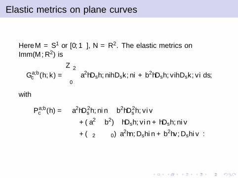
Elastic metrics on plane curves

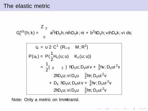
Here M = S1 or [0, 1π], N = R2. The elastic metrics onImm(M,R2) is

G a,bc (h, k) =

∫ 2π

0a2〈Dsh, n〉〈Dsk , n〉+ b2〈Dsh, v〉〈Dsk, v〉 ds,

with

Pa,bc (h) =− a2〈D2

s h, n〉n − b2〈D2s h, v〉v

+ (a2 − b2)κ(〈Dsh, v〉n + 〈Dsh, n〉v

)+ (δ2π − δ0)

(a2〈n,Dsh〉n + b2〈v ,Dsh〉v

).

Sobolev type metrics

Advantages of Sobolev type metrics:

1. Positive geodesic distance

2. Geodesic equations are well posed

3. Spaces are geodesically complete for p > dim(M)2 + 1.

[Bruveris, M, Mumford, 2013] for plane curves. A remark in [Ebin, Marsden, 1970], and [Bruveris, Meyer,

2014] for diffeomorphism groups.

Problems:

1. Analytic solutions to the geodesic equation?

2. Curvature of shape space with respect to these metrics?

3. Numerics are in general computational expensive

wellp.:Space:

geod. dist.:

p≥1/2

Diff(S1)

+:p> 12,−:p≤ 1

2

r-acts //

r-acts

$$

p≥1

Imm(S1,R2)−:p=0,+:p≥1

needs g

Diff(S1) ""

p≥1

Diffc (R2)

−:p< 12,+:p≥1

l-acts

(LDDMM)

oo

l-acts

(LDDMM)

wellp.:Space:

geod. dist.:

p≥0

Met(S1)+:p≥0

p≥1

Bi (S1,R2)

−:p=0,+:p≥1

Sobolev type metrics

Advantages of Sobolev type metrics:

1. Positive geodesic distance

2. Geodesic equations are well posed

3. Spaces are geodesically complete for p > dim(M)2 + 1.

[Bruveris, M, Mumford, 2013] for plane curves. A remark in [Ebin, Marsden, 1970], and [Bruveris, Meyer,

2014] for diffeomorphism groups.

Problems:

1. Analytic solutions to the geodesic equation?

2. Curvature of shape space with respect to these metrics?

3. Numerics are in general computational expensivewellp.:

Space:dist.:

p≥1Diff(M)

+:p>1,−:p< 12

r-acts //

r-acts

$$

p≥1Imm(M,N)−:p=0,+:p≥1

needs g

Diff(M)

##

p≥1Diffc (N)

−:p< 12,+:p≥1

l-acts

(LDDMM)

oo

l-acts

(LDDMM)

wellp.:Space:

dist.:

p=k,k∈NMet(M)

+:p≥0

p≥1Bi (M,N)−:p=0,+:p≥1

Geodesic equation.

The geodesic equation for a Sobolev-type metric GP onimmersions is given by

∇∂t ft =1

2P−1

(Adj(∇P)(ft , ft)

⊥ − 2.Tf .g(Pft ,∇ft)]

− g(Pft , ft).Trg (S))

− P−1(

(∇ft P)ft + Trg(g(∇ft ,Tf )

)Pft).

The geodesic equation written in terms of the momentum for aSobolev-type metric GP on Imm is given by:

p = Pft ⊗ vol(f ∗g)

∇∂t p =1

2

(Adj(∇P)(ft , ft)

⊥ − 2Tf .g(Pft ,∇ft)]

− g(Pft , ft) Trf∗g (S)

)⊗ vol(f ∗g)

WellposednessAssumption 1: P,∇P and Adj(∇P)⊥ are smooth sections of thebundles

L(T Imm; T Imm)

L2(T Imm; T Imm)

L2(T Imm; T Imm)

Imm Imm Imm,

respectively. Viewed locally in trivializ. of these bundles,

Pf h, (∇P)f (h, k),(

Adj(∇P)f (h, k))⊥

are pseudo-differentialoperators of order 2p in h, k separately. As mappings in f they arenon-linear, and we assume they are a composition of operators of thefollowing type:(a) Local operators of order l ≤ 2p, i.e., nonlinear differential operatorsA(f )(x) = A(x , ∇l f (x), ∇l−1f (x), . . . , ∇f (x), f (x))(b) Linear pseudo-differential operators of degrees li ,such that the total (top) order of the composition is ≤ 2p.Assumption 2: For each f ∈ Imm(M,N), the operator Pf is an ellipticpseudo-differential operator of order 2p for p > 0 which is positive andsymmetric with respect to the H0-metric on Imm, i.e.∫

M

g(Pf h, k) vol(g) =

∫M

g(h,Pf k) vol(g) for h, k ∈ Tf Imm.

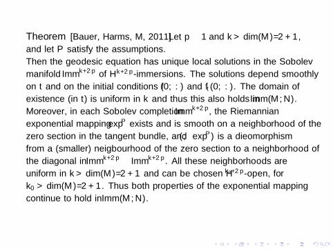
Theorem [Bauer, Harms, M, 2011] Let p ≥ 1 and k > dim(M)/2 + 1,

and let P satisfy the assumptions.

Then the geodesic equation has unique local solutions in the Sobolev

manifold Immk+2p of Hk+2p-immersions. The solutions depend smoothly

on t and on the initial conditions f (0, . ) and ft(0, . ). The domain of

existence (in t) is uniform in k and thus this also holds in Imm(M,N).

Moreover, in each Sobolev completion Immk+2p, the Riemannian

exponential mapping expP exists and is smooth on a neighborhood of the

zero section in the tangent bundle, and (π, expP) is a diffeomorphism

from a (smaller) neigbourhood of the zero section to a neighborhood of

the diagonal in Immk+2p × Immk+2p. All these neighborhoods are

uniform in k > dim(M)/2 + 1 and can be chosen Hk0+2p-open, for

k0 > dim(M)/2 + 1. Thus both properties of the exponential mapping

continue to hold in Imm(M,N).

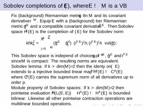
Sobolev completions of Γ(E ), where E → M is a VB

Fix (background) Riemannian metric g on M and its covariantderivative ∇M . Equip E with a (background) fiber Riemannianmetric gE and a compatible covariant derivative ∇E . Then Sobolevspace Hk(E ) is the completion of Γ(E ) for the Sobolev norm

‖h‖2k =

k∑j=0

∫M

(gE ⊗ g 0j )((∇E )jh, (∇E )jh

)vol(g).

This Sobolev space is independ of choices of g , ∇M , gE and ∇E

since M is compact: The resulting norms are equivalent.Sobolev lemma: If k > dim(M)/2 then the identy on Γ(E )extends to a injective bounded linear map Hk+p(E )→ Cp(E )where Cp(E ) carries the supremum norm of all derivatives up toorder p.Module property of Sobolev spaces: If k > dim(M)/2 thenpointwise evaluation Hk(L(E ,E ))× Hk(E )→ Hk(E ) is boundedbilinear. Likewise all other pointwise contraction operations aremultilinear bounded operations.

Proof of well-posedness

By assumption 1 the mapping Pf h is of order 2p in f and in hwhere f is the footpoint of h. Therefore f 7→ Pf extends to asmooth section of the smooth Sobolev bundle

L(T Immk+2p; T Immk | Immk+2p

)→ Immk+2p,

where T Immk | Immk+2p denotes the space of all Hk tangentvectors with foot point a Hk+2p immersion, i.e., the restriction ofthe bundle T Immk → Immk to Immk+2p ⊂ Immk .This means that Pf is a bounded linear operator

Pf ∈ L(Hk+2p(f ∗TN),Hk(f ∗TN)

)for f ∈ Immk+2p.

It is injective since it is positive. As an elliptic operator, it is anunbounded operator on the Hilbert completion of Tf Imm withrespect to the H0-metric, and a Fredholm operator Hk+2p → Hk

for each k . It is selfadjoint elliptic, so the index =0. Since it isinjective, it is thus also surjective.

By the implicit function theorem on Banach spaces, f 7→ P−1f is

then a smooth section of the smooth Sobolev bundle

L(T Immk | Immk+2p; T Immk+2p

)→ Immk+2p

As an inverse of an elliptic pseudodifferential operator, P−1f is also

an elliptic pseudo-differential operator of order −2p.

By assumption 1 again, (∇P)f (m, h) and(

Adj(∇P)f (m, h))⊥

areof order 2p in f ,m, h (locally). Therefore f 7→ Pf andf 7→ Adj(∇P)⊥ extend to smooth sections of the Sobolev bundle

L2(T Immk+2p; T Immk | Immk+2p

)→ Immk+2p

Using the module property of Sobolev spaces, one obtains that the”Christoffel symbols”

Γf (h, h) =1

2P−1

(Adj(∇P)(h, h)⊥ − 2.Tf .g(Ph,∇h)]

− g(Ph, h).Trg (S)− (∇hP)h − Trg(g(∇h,Tf )

)Ph)

extend to a smooth (C∞) section of the smooth Sobolev bundle

L2sym

(T Immk+2p; T Immk+2p

)→ Immk+2p

Thus h 7→ Γf (h, h) is a smooth quadratic mappingT Imm→ T Imm which extends to smooth quadratic mappingsT Immk+2p → T Immk+2p for each k ≥ dim(2)

2 + 1. The geodesic

equation ∇g∂t

ft = Γf (ft , ft) can be reformulated using the linear

connection C g : TN ×N TN → TTN (horizontal lift mapping) of∇g :

∂t ft = C(1

2Hf (ft , ft)− Kf (ft , ft), ft

).

The right-hand side is a smooth vector field on T Immk+2p, thegeodesic spray. Note that the restriction to T Immk+1+2p of thegeodesic spray on T Immk+2p equals the geodesic spray there. Bythe theory of smooth ODE’s on Banach spaces, the flow of thisvector field exists in T Immk+2p and is smooth in time and in theinitial condition, for all k ≥ dim(2)

2 + 1.It remains to show that the domain of existence is independent ofk . I omit this. QED

Sobolev metrics of order ≥ 2 on Imm(S1,R2) are complete

Theorem. [Bruveris, M, Mumford, 2014] Let n ≥ 2 and the metricG on Imm(S1,R2) be given by

Gc(h, k) =

∫S1

n∑j=0

aj〈D jsh,D j

sk〉ds ,

with aj ≥ 0 and a0, an 6= 0. Given initial conditions(c0, u0) ∈ T Imm(S1,R2) the solution of the geodesic equation

∂t

n∑j=0

(−1)j |c ′|D2js ct

= −a0

2|c ′|Ds (〈ct , ct〉v)

+n∑

k=1

2k−1∑j=1

(−1)k+j ak2|c ′|Ds

(〈D2k−j

s ct ,Djsct〉v

).

for the metric G with initial values (c0, u0) exists for all time.

Recall: ds = |c ′|dθ is arc-length measure, Ds = 1|c ′|∂θ is the

derivative with respect to arc-length, v = c ′/|c ′| is the unit lengthtangent vector to c and 〈 , 〉 is the Euclidean inner product on R2.

Thus if G is a Sobolev-type metric of order at least 2, so that∫S1

(|h|2 + |D2s h|2)ds ≤ C Gc(h, h),

then the Riemannian manifold (Imm(S1,R2),G ) is geodesicallycomplete. If the Sobolev-type metric is invariant under thereparameterization group Diff(S1), also the induced metric onshape space Imm(S1,R2)/Diff(S1) is geodesically complete.

The proof of this theorem is surprisingly difficult.

The elastic metric

G a,bc (h, k) =

∫ 2π

0a2〈Dsh, n〉〈Dsk , n〉+ b2〈Dsh, v〉〈Dsk, v〉 ds,

ct = u ∈ C∞(R>0 ×M,R2)

P(ut) = P(1

2Hc(u, u)− Kc(u, u))

=1

2(δ0 − δ2π)

(〈Dsu,Dsu〉v + 3

4〈v ,Dsu〉2v

− 2〈Dsu, v〉Dsu − 32〈n,Dsu〉2v

)+ Ds

(〈Dsu,Dsu〉v + 3

4〈v ,Dsu〉2v

− 2〈Dsu, v〉Dsu − 32〈n,Dsu〉2v

)Note: Only a metric on Imm/transl.

Representation of the elastic metrics

Aim: Represent the class of elastic metrics as the pullback metricof a flat metric on C∞(M,R2), i.e.: find a map

R : Imm(M,R2) 7→ C∞(M,Rn)

such that

G a,bc (h, k) = R∗〈h, k〉L2 = 〈TcR.h,TcR.k〉L2 .

[YounesMichorShahMumford2008] [SrivastavaKlassenJoshiJermyn2011]

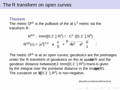
The R transform on open curves

TheoremThe metric G a,b is the pullback of the flat L2 metric via thetransform R:

Ra,b : Imm([0, 2π],R2)→ C∞([0, 2π],R3)

Ra,b(c) = |c ′|1/2

(a

(v0

)+√

4b2 − a2

(01

)).

The metric G a,b is flat on open curves, geodesics are the preimagesunder the R-transform of geodesics on the flat space im R and thegeodesic distance between c , c ∈ Imm([0, 2π],R2)/ trans is givenby the integral over the pointwise distance in the image Im(R).The curvature on B([0, 2π],R2) is non-negative.

[BauerBruverisMarslandMichor2014]

The R transform on open curves II

Image of R is characterized by the condition:

(4b2 − a2)(R21 (c) + R2

2 (c)) = a2R23 (c)

Define the flat cone

C a,b = q ∈ R3 : (4b2 − a2)(q21 + q2

2) = a2q23 , q3 > 0.

Then Im R = C∞(S1,C a,b). The inverse of R is given by:

R−1 : im R → Imm([0, 2π],R2)/ trans

R−1(q)(θ) = p0 +1

2ab

∫ θ

0|q(θ)|

(q1(θ)q2(θ)

)dθ .

The R transform on closed curves I

Characterize image using the inverse:

R−1(q)(θ) = p0 +1

2ab

∫ θ

0|q(θ)|

(q1(θ)q2(θ)

)dθ .

R−1(q)(θ) is closed iff

F (q) =

∫ 2π

0|q(θ)|

(q1(θ)q2(θ)

)dθ = 0

A basis of the orthogonal complement(TqC a,b

)⊥is given by the

two gradients gradL2Fi (q)

The R transform on closed curves II

TheoremThe image C a,b of the manifold of closed curves under theR-transform is a codimension 2 submanifold of the flat space

Im(R)open. A basis of the orthogonal complement(TqC a,b

)⊥is

given by the two vectors

U1(q) =1√

q21 + q2

2

2q21 + q2

2

q1q2

0

+2

a

√4b2 − a2

00q1

,

U2(q) =1√

q21 + q2

2

q1q2

q21 + 2q2

2

0

+2

a

√4b2 − a2

00q2

.

[BauerBruverisMarslandMichor2012]

compress and stretch

A geodesic Rectangle

Non-symmetric distances

I1 → I2 I2 → I1I1 I2 # iterations # points distance # iterations # points distance %diff

cat cow 28 456 7.339 33 462 8.729 15.9cat dog 36 475 8.027 102 455 10.060 20.2cat donkey 73 476 12.620 102 482 12.010 4.8cow donkey 32 452 7.959 26 511 7.915 0.6dog donkey 15 457 8.299 10 476 8.901 6.8

shark airplane 63 491 13.741 40 487 13.453 2.1

An example of a metric space with stronglynegatively curved regions

Diff(S2)r-acts //

r-acts $$

Imm(S2,R3)

needs gxx Diff(S2) ''

Diffc(R2)l-acts

(LDDMM)oo

l-acts

(LDDMM)xxMet(S2) Bi (S2,R3)

G Φf (h, k) =

∫M

Φ(f )g(h, k) vol(g)

[BauerHarmsMichor2012]

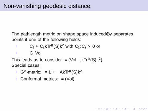
Non-vanishing geodesic distance

The pathlength metric on shape space induced by G Φ separatespoints if one of the following holds:

I Φ ≥ C1 + C2‖Trg (S)‖2 with C1,C2 > 0 or

I Φ ≥ C3 Vol

This leads us to consider Φ = Φ(Vol, ‖Trg (S)‖2).Special cases:

I GA-metric: Φ = 1 + A‖Trg (S)‖2

I Conformal metrics: Φ = Φ(Vol)

Geodesic equation on shape space Bi (M ,Rn), withΦ = Φ(Vol,Tr(L))

ft = a.ν,

at =1

Φ

[Φ

2a2 Tr(L)− 1

2Tr(L)

∫M

(∂1Φ)a2 vol(g)− 1

2a2∆(∂2Φ)

+ 2ag−1(d(∂2Φ), da) + (∂2Φ)‖da‖2g−1

+ (∂1Φ)a

∫M

Tr(L).a vol(g)− 1

2(∂2Φ) Tr(L2)a2

]

Sectional curvature on Bi

Chart for Bi centered at π(f0) so that π(f0) = 0 in this chart:

a ∈ C∞(M)←→ π(f0 + a.νf0).

For a linear 2-dim. subspace P ⊂ Tπ(f0)Bi spanned by a1, a1, thesectional curvature is defined as:

k(P) = −G Φπ(f0)

(Rπ(f0)(a1, a2)a1, a2

)‖a1‖2‖a2‖2 − G Φ

π(f0)(a1, a2)2, where

R0(a1, a2, a1, a2) = G Φ0 (R0(a1, a2)a1, a2) =

1

2d2G Φ

0 (a1, a1)(a2, a2) +1

2d2G Φ

0 (a2, a2)(a1, a1)

− d2G Φ0 (a1, a2)(a1, a2)

+ G Φ0 (Γ0(a1, a1), Γ0(a2, a2))− G Φ

0 (Γ0(a1, a2), Γ0(a1, a2)).

Sectional curvature on Bi for Φ = Vol

k(P) = − R0(a1, a2, a1, a2)

‖a1‖2‖a2‖2 − G Φπ(f0)(a1, a2)2

, where

R0(a1, a2, a1, a2) = −1

2Vol

∫M‖a1da2 − a2da1‖2

g−1 vol(g)

+1

4 VolTr(L)2

(a2

1.a22 − a1.a2

2)

+1

4

(a2

1.Tr(L)2a22 − 2a1.a2.Tr(L)2a1.a2 + a2

2.Tr(L)2a21

)− 3

4 Vol

(a2

1.Tr(L)a22 − 2a1.a2.Tr(L)a1.Tr(L)a2 + a2

2.Tr(L)a12)

+1

2

(a2

1.Trg ((da2)2)− 2a1.a2.Trg (da1.da2) + a22Trg ((da1)2)

)− 1

2

(a2

1.a22.Tr(L2)− 2.a1.a2.a1.a2.Tr(L2) + a2

2.a21.Tr(L2)

).

Sectional curvature on Bi for Φ = 1 + ATr(L)2

k(P) = − R0(a1, a2, a1, a2)

‖a1‖2‖a2‖2 − G Φπ(f0)(a1, a2)2

, where

R0(a1, a2, a1, a2) =

∫M

A(a1∆a2 − a2∆a1)2 vol(g)

+

∫M

2A Tr(L)g 02

((a1da2 − a2da1)⊗ (a1da2 − a2da1), s

)vol(g)

+

∫M

1

1 + A Tr(L)2

[− 4A2g−1

(d Tr(L), a1da2 − a2da1

)2

−(1

2

(1 + A Tr(L)2

)2+ 2A2 Tr(L)∆(Tr(L)) + 2A2 Tr(L2) Tr(L)2

)·

· ‖a1da2 − a2da1‖2g−1 + (2A2 Tr(L)2)‖da1 ∧ da2‖2

g20

+ (8A2 Tr(L))g 02

(d Tr(L)⊗ (a1da2 − a2da1), da1 ∧ da2

)]vol(g)

Negative Curvature: A toy example

Movies: Ex1: Φ = 1 + .4 Tr(L)2 Ex2: Φ = eVol Ex3: Φ = eVol

Another toy example

G Φf (h, k) =

∫T2 g((1 + ∆)h, k) vol(g) on Imm(T2,R3):

[BauerBruveris2011]

Right invariant Riemannian geometries onDiffeomorphism groups.

For M = N the space Emb(M,M) equals the diffeomorphismgroup of M. An operator P ∈ Γ

(L(T Emb; T Emb)

)that is

invariant under reparametrizations induces a right-invariantRiemannian metric on this space. Thus one gets the geodesicequation for right-invariant Sobolev metrics on diffeomorphismgroups and well-posedness of this equation. The geodesic equationon Diff(M) in terms of the momentum p is given by

p = Pft ⊗ vol(g),

∇∂t p = −Tf .g(Pft ,∇ft)] ⊗ vol(g).

Note that this equation is not right-trivialized, in contrast to theequation given in [Arnold 1966]. The special case of theorem nowreads as follows:

Theorem. [Bauer, Harms, M, 2011] Let p ≥ 1 and k > dim(M)2 + 1 and

let P satisfy the assumptions.

The initial value problem for the geodesic equation has unique local

solutions in the Sobolev manifold Diffk+2p of Hk+2p-diffeomorphisms.

The solutions depend smoothly on t and on the initial conditions f (0, . )

and ft(0, . ). The domain of existence (in t) is uniform in k and thus this

also holds in Diff(M).

Moreover, in each Sobolev completion Diffk+2p, the Riemannian

exponential mapping expP exists and is smooth on a neighborhood of the

zero section in the tangent bundle, and (π, expP) is a diffeomorphism

from a (smaller) neigbourhood of the zero section to a neighborhood of

the diagonal in Diffk+2p ×Diffk+2p. All these neighborhoods are uniform

in k > dim(M)/2 + 1 and can be chosen Hk0+2p-open, for

k0 > dim(M)/2 + 1. Thus both properties of the exponential mapping

continue to hold in Diff(M).

Arnold’s formula for geodesics on Lie groups: Notation

Let G be a regular convenient Lie group, with Lie algebra g. Letµ : G × G → G be the group multiplication, µx the left translationand µy the right translation, µx(y) = µy (x) = xy = µ(x , y).

Let L,R : g→ X(G ) be the left- and right-invariant vector fieldmappings, given by LX (g) = Te(µg ).X and RX = Te(µg ).X , resp.They are related by LX (g) = RAd(g)X (g). Their flows are given by

FlLXt (g) = g . exp(tX ) = µexp(tX )(g),

FlRXt (g) = exp(tX ).g = µexp(tX )(g).

The right Maurer–Cartan form κ = κr ∈ Ω1(G , g) is given byκx(ξ) := Tx(µx

−1) · ξ.

The left Maurer–Cartan form κl ∈ Ω1(G , g) is given byκx(ξ) := Tx(µx−1) · ξ.

κr satisfies the left Maurer-Cartan equation dκ− 12 [κ, κ]∧g = 0,

where [ , ]∧ denotes the wedge product of g-valued forms on Ginduced by the Lie bracket. Note that 1

2 [κ, κ]∧(ξ, η) = [κ(ξ), κ(η)].κl satisfies the right Maurer-Cartan equation dκ+ 1

2 [κ, κ]∧g = 0.

Proof: Evaluate dκr on right invariant vector fields RX ,RY forX ,Y ∈ g.

(dκr )(RX ,RY ) = RX (κr (RY ))− RY (κr (RX ))− κr ([RX ,RY ])

= RX (Y )− RY (X ) + [X ,Y ] = 0− 0 + [κr (RX ), κr (RY )].

The (exterior) derivative of the function Ad : G → GL(g) can beexpressed by

d Ad = Ad .(ad κl) = (ad κr ).Ad

since we haved Ad(Tµg .X ) = d

dt |0 Ad(g . exp(tX )) = Ad(g). ad(κl(Tµg .X )).

Geodesics of a Right-Invariant Metric on a Lie Group

Let γ = g× g→ R be a positive-definite bounded (weak) innerproduct. Then

γx(ξ, η) = γ(T (µx

−1) · ξ, T (µx

−1) · η

)= γ

(κ(ξ), κ(η)

)is a right-invariant (weak) Riemannian metric on G . Denote byγ : g→ g∗ the mapping induced by γ, and by 〈α,X 〉g the dualityevaluation between α ∈ g∗ and X ∈ g.Let g : [a, b]→ G be a smooth curve. The velocity field of g ,viewed in the right trivializations, coincides with the rightlogarithmic derivative

δr (g) = T (µg−1

) · ∂tg = κ(∂tg) = (g∗κ)(∂t).

The energy of the curve g(t) is given by

E (g) =1

2

∫ b

aγg (g ′, g ′)dt =

1

2

∫ b

aγ((g∗κ)(∂t), (g∗κ)(∂t)

)dt.

For a variation g(s, t) with fixed endpoints we then use that

d(g∗κ)(∂t , ∂s) = ∂t(g∗κ(∂s))− ∂s(g∗κ(∂t))− 0,

partial integration and the left Maurer–Cartan equation to obtain

∂sE (g) =1

2

∫ b

a

2γ(∂s(g∗κ)(∂t), (g∗κ)(∂t)

)dt

=

∫ b

a

γ(∂t(g∗κ)(∂s)− d(g∗κ)(∂t , ∂s), (g∗κ)(∂t)

)dt

= −∫ b

a

γ((g∗κ)(∂s), ∂t(g∗κ)(∂t)

)dt

−∫ b

a

γ([(g∗κ)(∂t), (g∗κ)(∂s)], (g∗κ)(∂t)

)dt

= −∫ b

a

⟨γ(∂t(g∗κ)(∂t)), (g∗κ)(∂s)

⟩g

dt

−∫ b

a

⟨γ((g∗κ)(∂t)), ad(g∗κ)(∂t)(g∗κ)(∂s)

⟩g

dt

= −∫ b

a

⟨γ(∂t(g∗κ)(∂t)) + (ad(g∗κ)(∂t))

∗γ((g∗κ)(∂t)), (g∗κ)(∂s)⟩g

dt.

Thus the curve g(0, t) is critical for the energy if and only if

γ(∂t(g∗κ)(∂t)) + (ad(g∗κ)(∂t))∗γ((g∗κ)(∂t)) = 0.

In terms of the right logarithmic derivative u : [a, b]→ g ofg : [a, b]→ G , given by u(t) := g∗κ(∂t) = Tg(t)(µg(t)−1

) · g ′(t),the geodesic equation has the expression

∂tu = − γ−1 ad(u)∗ γ(u) (1)

Thus the geodesic equation exists in general if and only ifad(X )∗γ(X ) is in the image of γ : g→ g∗, i.e.

ad(X )∗γ(X ) ∈ γ(g) (2)

for every X ∈ X. Condition (2) then leads to the existence of theChristoffel symbols. [Arnold 1966] has the more restrictivecondition ad(X )∗γ(Y ) ∈ γ ∈ g. The geodesic equation for themomentum p := γ(u):

pt = − ad(γ−1(p))∗p.

Soon we shall encounter situations where only the more generalcondition is satisfied, but where the usual transpose ad>(X ) ofad(X ),

ad>(X ) := γ−1 ad∗X γ

does not exist for all X .

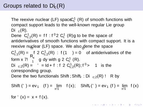
Groups related to Diffc(R)

The reflexive nuclear (LF) space C∞c (R) of smooth functions withcompact support leads to the well-known regular Lie groupDiffc(R).Define C∞c,2(R) = f : f ′ ∈ C∞c (R) to be the space ofantiderivatives of smooth functions with compact support. It is areflexive nuclear (LF) space. We also define the space

C∞c,1(R) =

f ∈ C∞c,2(R) : f (−∞) = 0

of antiderivatives of the

form x 7→∫ x−∞ g dy with g ∈ C∞c (R).

Diffc,2(R) =ϕ = Id +f : f ∈ C∞c,2(R), f ′ > −1

is the

corresponding group.Define the two functionals Shift`,Shiftr : Diffc,2(R)→ R by

Shift`(ϕ) = ev−∞(f ) = limx→−∞

f (x), Shiftr (ϕ) = ev∞(f ) = limx→∞

f (x)

for ϕ(x) = x + f (x).

Then the short exact sequence of smooth homomorphisms of Liegroups

Diffc(R) // // Diffc,2(R)(Shift`,Shiftr ) // // (R2,+)

describes a semidirect product, where a smooth homomorphicsection s : R2 → Diffc,2(R) is given by the composition of flowss(a, b) = FlX`a FlXr

b for the vectorfields X` = f`∂x , Xr = fr∂x with[X`,Xr ] = 0 where f`, fr ∈ C∞(R, [0, 1]) satisfy

f`(x) =

1 for x ≤ −1

0 for x ≥ 0,fr (x) =

0 for x ≤ 0

1 for x ≥ 1.(3)

The normal subgroupDiffc,1(R) = ker(Shift`) = ϕ = Id +f : f ∈ C∞c,1(R), f ′ > −1 ofdiffeomorphisms which have no shift at −∞ will play an importantrole later on.

Some diffeomorphism groups on R

We have the following smooth injective group homomorphisms:

Diffc(R) //

DiffS(R)

// DiffW∞,1(R)

Diffc,1(R) //

DiffS1(R) //

DiffW∞,11

(R)

Diffc,2(R) // DiffS2(R) // Diff

W∞,12(R) // DiffB(R)

Each group is a normal subgroup in any other in which it iscontained, in particular in DiffB(R).For S and W∞,1 this works the same as for C∞c . For H∞ = W∞,2

it is surprisingly more subtle.

Solving the Hunter-Saxton equation: The setting

We will denote by A(R) any of the spaces C∞c (R), S(R) orW∞,1(R) and by DiffA(R) the corresponding groups Diffc(R),DiffS(R) or DiffW∞,1(R).Similarly A1(R) will denote any of the spaces C∞c,1(R), S1(R) or

W∞,11 (R) and DiffA1(R) the corresponding groups Diffc,1(R),

DiffS1(R) or DiffW∞,11

(R).

The H1-metric. For DiffA(R) and DiffA1(R) the homogeneousH1-metric is given by

Gϕ(X ϕ,Y ϕ) = GId(X ,Y ) =

∫R

X ′(x)Y ′(x) dx ,

where X ,Y are elements of the Lie algebra A(R) or A1(R). Weshall also use the notation

〈·, ·〉H1 := G (·, ·) .

Theorem

On DiffA1(R) the geodesic equation is the Hunter-Saxton equation

(ϕt) ϕ−1 = u ut = −uux +1

2

∫ x

−∞(ux(z))2 dz ,

and the induced geodesic distance is positive.On the other hand the geodesic equation does not exist on thesubgroups DiffA(R), since the adjoint ad(X )∗GId(X ) does not liein GId(A(R)) for all X ∈ A(R).One obtains the classical form of the Hunter-Saxton equation bydifferentiating:

utx = −uuxx −1

2u2x ,

Note that DiffA(R) is a natural example of a non-robustRiemannian manifold.

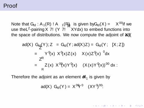
Proof

Note that GId : A1(R)→ A1(R)∗ is given by GId(X ) = −X ′′ if weuse the L2-pairing X 7→ (Y 7→

∫XYdx) to embed functions into

the space of distributions. We now compute the adjoint of ad(X ):⟨ad(X )∗GId(Y ),Z

⟩= GId(Y , ad(X )Z ) = GId(Y ,−[X ,Z ])

=

∫R

Y ′(x)(X ′(x)Z (x)− X (x)Z ′(x)

)′dx

=

∫R

Z (x)(X ′′(x)Y ′(x)− (X (x)Y ′(x))′′

)dx .

Therefore the adjoint as an element of A∗1 is given by

ad(X )∗GId(Y ) = X ′′Y ′ − (XY ′)′′ .

For X = Y we can rewrite this as

ad(X )∗GId(X ) = 12

((X ′2)′ − (X 2)′′′

)=

1

2

(∫ x

−∞X ′(y)2 dy − (X 2)′

)′′=

1

2GId

(−∫ x

−∞X ′(y)2 dy + (X 2)′

).

If X ∈ A1(R) then the function −12

∫ x−∞ X ′(y)2 dy + 1

2 (X 2)′ isagain an element of A1(R). This follows immediately from thedefinition of A1(R). Therefore the geodesic equation exists onDiffA1(R) and is as given.However if X ∈ A(R), a neccessary condition for∫ x−∞(X ′(y))2dy ∈ A(R) would be

∫∞−∞ X ′(y)2dy = 0, which would

imply X ′ = 0. Thus the geodesic equation does not exist on A(R).The positivity of geodesic distance will follow from the explicitformula for geodesic distance below. QED.

Theorem.

[BBM2014] [A version for Diff (S1) is by J.Lenells 2007,08,11]We define the R-map by:

R :

DiffA1(R)→ A

(R,R>−2

)⊂ A(R,R)

ϕ 7→ 2((ϕ′)1/2 − 1

).

The R-map is invertible with inverse

R−1 :

A(R,R>−2

)→ DiffA1(R)

γ 7→ x +1

4

∫ x

−∞γ2 + 4γ dx .

The pull-back of the flat L2-metric via R is the H1-metric onDiffA(R), i.e.,

R∗〈·, ·〉L2 = 〈·, ·〉H1 .

Thus the space(DiffA1(R), H1

)is a flat space in the sense of

Riemannian geometry.Here 〈·, ·〉L2 denotes the L2-inner product on A(R) with constantvolume dx .

Proof

To compute the pullback of the L2-metric via the R-map we firstneed to calculate its tangent mapping. For this leth = X ϕ ∈ TϕDiffA1(R) and let t 7→ ψ(t) be a smooth curve inDiffA1(R) with ψ(0) = Id and ∂t |0ψ(t) = X . We have:

TϕR.h = ∂t |0R(ψ(t) ϕ) = ∂t |02(

((ψ(t) ϕ)x)1/2 − 1)

= ∂t |02((ψ(t)x ϕ)ϕx)1/2

= 2(ϕx)1/2∂t |0((ψ(t)x)1/2 ϕ) = (ϕx)1/2( ψtx(0)

(ψ(0)x)−1/2 ϕ)

= (ϕx)1/2(X ′ ϕ) = (ϕ′)1/2(X ′ ϕ) .

Using this formula we have for h = X1 ϕ, k = X2 ϕ:

R∗〈h, k〉L2 = 〈TϕR.h,TϕR.k〉L2 =

∫R

X ′1(x)X ′2(x) dx = 〈h, k〉H1 QED

Corollary

Given ϕ0, ϕ1 ∈ DiffA1(R) the geodesic ϕ(t, x) connecting them isgiven by

ϕ(t, x) = R−1(

(1− t)R(ϕ0) + tR(ϕ1))

(x)

and their geodesic distance is

d(ϕ0, ϕ1)2 = 4

∫R

((ϕ′1)1/2 − (ϕ′0)1/2

)2dx .

But this construction shows much more: For S1, C∞1 , and even formany kinds of Denjoy-Carleman ultradifferentiable model spaces(not explained here). This shows that Sobolev space methods fortreating nonlinear PDEs is not the only method.

Corollary: The metric space(DiffA1(R), H1

)is path-connected

and geodesically convex but not geodesically complete. Inparticular, for every ϕ0 ∈ DiffA1(R) and h ∈ Tϕ0 DiffA1(R), h 6= 0there exists a time T ∈ R such that ϕ(t, ·) is a geodesic for|t| < |T | starting at ϕ0 with ϕt(0) = h, but ϕx(T , x) = 0 for somex ∈ R.Theorem: The square root representation on the diffeomorphismgroup DiffA(R) is a bijective mapping, given by:

R :

DiffA(R)→

(Im(R), ‖ · ‖L2

)⊂(A(R,R>−2

), ‖ · ‖L2

)ϕ 7→ 2

((ϕ′)1/2 − 1

).

The pull-back of the restriction of the flat L2-metric to Im(R) via Ris again the homogeneous Sobolev metric of order one. The imageof the R-map is the splitting submanifold of A(R,R>−2) given by:

Im(R) =γ ∈ A(R,R>−2) : F (γ) :=

∫Rγ(γ + 4

)dx = 0

.

On the space DiffA(R) the geodesic equation does not exist. Still:Corollary: The geodesic distance dA on DiffA(R) coincides withthe restriction of dA1 to DiffA(R), i.e., for ϕ0, ϕ1 ∈ DiffA(R) wehave

dA(ϕ0, ϕ1) = dA1(ϕ0, ϕ1) .

Continuing Geodesics Beyond the Group, or How Solutionsof the Hunter–Saxton Equation Blow Up

Consider a straight line γ(t) = γ0 + tγ1 in A(R,R). Thenγ(t) ∈ A(R,R>−2) precisely for t in an open interval (t0, t1) whichis finite at least on one side, say, at t1 <∞. Note that

ϕ(t)(x) := R−1(γ(t))(x) = x +1

4

∫ x

−∞γ2(t)(u) + 4γ(t)(u) du

makes sense for all t, that ϕ(t) : R→ R is smooth and thatϕ(t)′(x) ≥ 0 for all x and t; thus, ϕ(t) is monotonenon-decreasing. Moreover, ϕ(t) is proper and surjective since γ(t)vanishes at −∞ and ∞. Let

MonA1(R) :=

Id +f : f ∈ A1(R,R), f ′ ≥ −1

be the monoid (under composition) of all such functions.

For γ ∈ A(R,R) let x(γ) := minx ∈ R ∪ ∞ : γ(x) = −2.Then for the line γ(t) from above we see that x(γ(t)) <∞ for allt > t1. Thus, if the ‘geodesic’ ϕ(t) leaves the diffeomorphismgroup at t1, it never comes back but stays insideMonA1(R) \ DiffA1(R) for the rest of its life. In this sense,MonA1(R) is a geodesic completion of DiffA1(R), andMonA1(R) \ DiffA1(R) is the boundary.What happens to the corresponding solutionu(t, x) = ϕt(t, ϕ(t)−1(x)) of the HS equation? In certain points ithas infinite derivative, it may be multivalued, or its graph cancontain whole vertical intervals. If we replace an elementϕ ∈ MonA1(R) by its graph (x , ϕ(x)) : x ∈ R ⊂ R we get asmooth ‘monotone’ submanifold, a smooth monotone relation.The inverse ϕ−1 is then also a smooth monotone relation. Thent 7→ (x , u(t, x)) : x ∈ R is a (smooth) curve of relations.Checking that it satisfies the HS equation is an exercise left for theinterested reader. What we have described here is the flowcompletion of the HS equation in the spirit of [KhesinMichor2004].

Soliton-Like Solutions of the Hunter Saxton equation

For a right-invariant metric G on a diffeomorphism group one canask whether (generalized) solutions u(t) = ϕt(t) ϕ(t)−1 existsuch that the momenta G (u(t)) =: p(t) are distributions withfinite support. Here the geodesic ϕ(t) may exist only in somesuitable Sobolev completion of the diffeomorphism group. By thegeneral theory, the momentum Ad(ϕ(t))∗p(t) = ϕ(t)∗p(t) = p(0)is constant. In other words,

p(t) = (ϕ(t)−1)∗p(0) = ϕ(t)∗p(0),

i.e., the momentum is carried forward by the flow and remains inthe space of distributions with finite support. The infinitesimalversion (take ∂t of the last expression) is

pt(t) = −Lu(t)p(t) = − adu(t)∗ p(t).

The space of N-solitons of order 0 consists of momenta of theform py ,a =

∑Ni=1 aiδyi with (y , a) ∈ R2N . Consider an initial

soliton p0 = G (u0) = −u′′0 =∑N

i=1 ai δyi with y1 < y2 < · · · < yN .Let H be the Heaviside function

H(x) =

0, x < 0,12 , x = 0,

1, x > 0,

and D(x) = 0 for x ≤ 0 and D(x) = x for x > 0. We will see laterwhy the choice H(0) = 1

2 is the most natural one; note that thebehavior is called the Gibbs phenomenon. With these functions wecan write

u′′0 (x) = −N∑i=1

aiδyi (x)

u′0(x) = −N∑i=1

aiH(x − yi )

u0(x) = −N∑i=1

aiD(x − yi ).

We will assume henceforth that∑N

i=1 ai = 0. Then u0(x) isconstant for x > yN and thus u0 ∈ H1

1 (R); with a slight abuse ofnotation we assume that H1

1 (R) is defined similarly to H∞1 (R).Defining Si =

∑ij=1 aj we can write

u′0(x) = −N∑i=1

Si (H(x − yi )− H(x − yi+1)) .

This formula will be useful becausesupp(H(.− yi )− H(.− yi+1)) = [yi , yi+1].The evolution of the geodesic u(t) with initial value u(0) = u0 canbe described by a system of ordinary differential equations (ODEs)for the variables (y , a).Theorem The map (y , a) 7→

∑Ni=1 aiδyi is a Poisson map between

the canonical symplectic structure on R2N and the Lie–Poissonstructure on the dual T ∗Id DiffA(R) of the Lie algebra.

In particular, this means that the ODEs for (y , a) are Hamilton’sequations for the pullback Hamiltonian

E (y , a) =1

2GId(u(y ,a), u(y ,a)),

with u(y ,a) = G−1(∑N

i=1 aiδyi ) = −∑N

i=1 aiD(.− yi ). We canobtain the more explicit expression

E (y , a) =1

2

∫R

(u(y ,a)(x)′

)2dx =

1

2

∫R

(N∑i=1

Si1[yi ,yi+1]

)2

dx

=1

2

N∑i=1

S2i (yi+1 − yi ).

Hamilton’s equations yi = ∂E/∂ai , ai = −∂E/∂yi are in this case

yi (t) =N−1∑j=i

Si (t)(yi+1(t)− yi (t)),

ai (t) =1

2

(Si (t)2 − Si−1(t)2

).

Using the R-map we can find explicit solutions for these equationsas follows. Let us write ai (0) = ai and yi (0) = yi . The geodesicwith initial velocity u0 is given by

ϕ(t, x) = x +1

4

∫ x

−∞t2(u′0(y))2 + 4tu′0(y) dy

u(t, x) = u0(ϕ−1(t, x)) +t

2

∫ ϕ−1(t,x)

−∞u′0(y)2 dy .

First note that

ϕ′(t, x) =(

1 +t

2u′0(x)

)2

u′(t, z) =u′0(ϕ−1(t, z)

)1 + t

2 u′0 (ϕ−1(t, z)).

Using the identity H(ϕ−1(t, z)− yi ) = H(z − ϕ(t, yi )) we obtain

u′0(ϕ−1(t, z)

)= −

N∑i=1

aiH (z − ϕ(t, yi )) ,

and thus (u′0(ϕ−1(t, z)

))′= −

N∑i=1

aiδϕ(t,yi )(z).

Combining these we obtain

u′′(t, z) =1(

1 + t2 u′0 (ϕ−1(t, z))

)2

(−

N∑i=1

aiδϕ(t,yi )(z)

)

=N∑i=1

−ai(1 + t

2 u′0(yi ))2δϕ(t,yi )(z).

From here we can read off the solution of Hamilton’s equations

yi (t) = ϕ(t, yi )

ai (t) = −ai(1 + t

2 u′0(yi ))−2

.

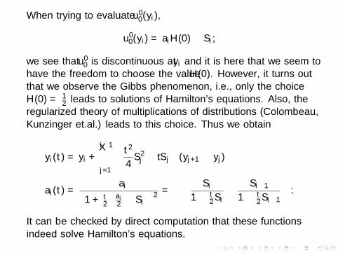
When trying to evaluate u′0(yi ),

u′0(yi ) = aiH(0)− Si ,

we see that u′0 is discontinuous at yi and it is here that we seem tohave the freedom to choose the value H(0). However, it turns outthat we observe the Gibbs phenomenon, i.e., only the choiceH(0) = 1

2 leads to solutions of Hamilton’s equations. Also, theregularized theory of multiplications of distributions (Colombeau,Kunzinger et.al.) leads to this choice. Thus we obtain

yi (t) = yi +i−1∑j=1

(t2

4S2j − tSj

)(yj+1 − yj)

ai (t) =−ai(

1 + t2

(ai2 − Si

))2= −

(Si

1− t2 Si− Si−1

1− t2 Si−1

).

It can be checked by direct computation that these functionsindeed solve Hamilton’s equations.

Riemannian geometries on spaces of Riemannian metricsand pulling them back to diffeomorphism groups.

Diff(M)r-acts //

r-acts

%%Diff(M,µ)

Imm(M,N)

needs gxx Diff(M) &&

DiffA(N)

r-acts

l-acts

(LDDMM)oo

l-acts

(LDDMM)xxMet(M)

Diff(M) %% %%

Bi (M,N)

needs gxxVol1+(M) Met(M)

Diff(M) Met(N)

Weak Riemann metrics on Met(M)

All of them are Diff(M)-invariant; natural, tautological.

Gg (h, k) =

∫M

g 02 (h, k) vol(g) =

∫Tr(g−1hg−1k) vol(g), L2-metr.

or = Φ(Vol(g))

∫M

g 02 (h, k) vol(g) conformal

or =

∫M

Φ(Scalg ).g 02 (h, k) vol(g) curvature modified

or =

∫M

g 02 ((1 + ∆g )ph, k) vol(g) Sobolev order p

or =

∫M

(g 0

2 (h, k) + g 03 (∇gh,∇gk) + . . .

+ g 0p ((∇g )ph, (∇g )pk)

)vol(g)

where Φ is a suitable real-valued function, Vol =∫M vol(g) is the

total volume of (M, g), Scal is the scalar curvature of (M, g), andwhere g 0

2 is the induced metric on(0

2

)-tensors.

The L2-metric on the space of all Riemann metrics

[Ebin 1970]. Geodesics and curvature [Freed Groisser 1989].[Gil-Medrano Michor 1991] for non-compact M. [Clarke 2009]showed that geodesic distance for the L2-metric is positive, and hedetermined the metric completion of Met(M).The geodesic equation is completely decoupled from space, it is anODE:

gtt = gtg−1gt + 1

4 Tr(g−1gtg−1gt) g − 1

2 Tr(g−1gt) gt

exp0(A) = 2n log

((1 + 1

4 Tr(A))2 + n16 Tr(A2

0))

Id

+4√

n Tr(A20)

arctan

(√n Tr(A2

0)

4 + Tr(A)

)A0.

Back to the the general metric on Met(M).

We describe all these metrics uniformly as

GPg (h, k) =

∫M

g 02 (Pgh, k) vol(g)

=

∫M

Tr(g−1.Pg (h).g−1.k) vol(g),

wherePg : Γ(S2T ∗M)→ Γ(S2T ∗M)

is a positive, symmetric, bijective pseudo-differential operator oforder 2p, p ≥ 0, depending smoothly on the metric g , and alsoDiff(M)-equivariantly:

ϕ∗ Pg = Pϕ∗g ϕ∗

The geodesic equation in this notation:

gtt = P−1[(D(g ,.)Pgt)

∗(gt) +1

4.g .Tr(g−1.Pgt .g

−1.gt)

+1

2gt .g

−1.Pgt +1

2Pgt .g

−1.gt − (D(g ,gt)P)gt

− 1

2Tr(g−1.gt).Pgt

]We can rewrite this equation to get it in a slightly more compact

form:

(Pgt)t = (D(g ,gt)P)gt + Pgtt

= (D(g ,.)Pgt)∗(gt) +

1

4.g .Tr(g−1.Pgt .g

−1.gt)

+1

2gt .g

−1.Pgt +1

2Pgt .g

−1.gt −1

2Tr(g−1.gt).Pgt

Well posedness of geodesic equation.

Assumptions Let Pg (h), P−1g (k) and (D(g ,.)Ph)∗(m) be linear

pseudo-differential operators of order 2p in m, h and of order −2p in kfor some p ≥ 0.As mappings in the foot point g, we assume that all mappings arenon-linear, and that they are a composition of operators of the followingtype:(a) Non-linear differential operators of order l ≤ 2p, i.e.,

A(g)(x) = A(x , g(x), (∇g)(x), . . . , (∇lg)(x)

),

(b) Linear pseudo-differential operators of order ≤ 2p,

such that the total (top) order of the composition is ≤ 2p.

Since h 7→ Pgh induces a weak inner product, it is a symmetric and

injective pseudodifferential operator. We assume that it is elliptic and

selfadjoint. Then it is Fredholm and has vanishing index. Thus it is

invertible and g 7→ P−1g is smooth

Hk(S2+T ∗M)→ L(Hk(S2T ∗M),Hk+2p(S2T ∗M)) by the implicit

function theorem on Banach spaces.

Theorem. [Bauer, Harms, M. 2011] Let the assumptions above hold.

Then for k > dim(M)2 , the initial value problem for the geodesic equation

has unique local solutions in the Sobolev manifold Metk+2p(M) of

Hk+2p-metrics. The solutions depend C∞ on t and on the initial

conditions g(0, . ) ∈ Metk+2p(M) and gt(0, . ) ∈ Hk+2p(S2T ∗M). The

domain of existence (in t) is uniform in k and thus this also holds in

Met(M).

Moreover, in each Sobolev completion Metk+2p(M), the Riemannian

exponential mapping expP exists and is smooth on a neighborhood of the

zero section in the tangent bundle, and (π, expP) is a diffeomorphism

from a (smaller) neighborhood of the zero section to a neighborhood of

the diagonal in Metk+2p(M)×Metk+2p(M). All these neighborhoods are

uniform in k > dim(M)2 and can be chosen Hk0+2p-open, where

k0 >dim(M)

2 . Thus all properties of the exponential mapping continue to

hold in Met(M).

Conserved Quantities on Met(M).

Right action of Diff(M) on Met(M) given by

(g , φ) 7→ φ∗g .

Fundamental vector field (infinitesimal action):

ζX (g) = LXg = −2 Sym∇(g(X )).

If metric GP is invariant, we have the following conservedquantities

const = GP(gt , ζX (g))

= −2

∫M

g 01

(∇∗ Sym Pgt , g(X )

)vol(g)

= −2

∫M

g(g−1∇∗Pgt ,X

)vol(g)

Since this holds for all vector fields X ,

(∇∗Pgt) vol(g) ∈ Γ(T ∗M ⊗M vol(M)) is const. in t.

For which metric is the Ricci flow a gradient flow

Met(M) is convex and open subset, thus contractible. A necessaryand sufficient condition for Ricci curvature to be a gradient vectorfield with respect to the GP -metric is that the following exteriorderivative vanishes:(dGP(Ric, ·)

)(h, k) = hGP(Ric, k)− kGP(Ric, h)− GP(Ric, [h, k]) = 0.

It suffices to look at constant vector fields h, k , in which case[h, k] = 0. We have

hGP(Ric, k)− kGP(Ric, h)

=

∫ (− Tr

(g−1hg−1(P Ric)g−1k

)+ Tr

(g−1kg−1(P Ric)g−1h

)+ Tr

(g−1Dg ,h(P Ric)g−1k

)− Tr

(g−1Dg ,k(P Ric)g−1h

)− Tr

(g−1(P Ric)g−1hg−1k

)+ Tr

(g−1(P Ric)g−1kg−1h

)+

1

2Tr(g−1(P Ric)g−1k

)Tr(g−1h)− 1

2Tr(g−1(P Ric)g−1h

)Tr(g−1k)

)vol(g).

Some terms in this formula cancel out because for symmetricA,B,C one has

Tr(ABC ) = Tr((ABC )>) = Tr(C>B>A>) = Tr(A>C>B>) = Tr(ACB).

Therefore

hGP( Ric, k)− kGP(Ric, h)

=

∫ (Tr(g−1Dg ,h(P Ric)g−1k

)− Tr

(g−1Dg ,k(P Ric)g−1h

)+

1

2Tr(g−1(P Ric)g−1k

)Tr(g−1h)

− 1

2Tr(g−1(P Ric)g−1h

)Tr(g−1k)

)vol(g).

We write Dg ,h(P Ric) = Q(h) for some differential operator Qmapping symmetric two-tensors to themselves and Q∗ for theadjoint of Q with respect to

∫M g 0

2 (h, k) vol(g).

hGP(Ric, k)− kGP(Ric, h)

=

∫ (g 0

2

(Q(h), k

)− g 0

2

(Q(k), h

)+

1

2g 0

2

(P Ric, k

)Tr(g−1h)− 1

2g 0

2

(P Ric, h

)Tr(g−1k)

)vol(g)

=

∫g 0

2

(Q(h)− Q∗(h) +

1

2(P Ric).Tr(g−1h)− 1

2g .g 0

2

(P Ric, h

), k)

vol(g).

We have proved:Lemma. The Ricci vector field Ric is a gradient field for theGP -metric if and only if the equation

2(Q(h)− Q∗(h)

)+ (P Ric).Tr(g−1h)− g .g 0

2

(P Ric, h

)= 0,

with Q(h) = Qg (h) = Dg ,h(Pg Ricg ),

is satisfied for all g ∈ Met(M) and and all symmetric(0

2

)-tensors h.

None of the specific metrics mentioned here satisfies the Lemma ingeneral dimension. Note that the Lemma is trivially satisfied indimension dim(M) = 1. In dimension 2 the equationRicg = 1

2 Scalg holds and the operator Pgh = 2 Scal−1g h satisfies

equation (1) on the open subset g : Scalg 6= 0. Generally,equation (1) is satisfied if Pg Ricg = g , but this cannot hold on thespace of all metrics if dim(M) > 2.

On Rn: DiffA(Rn) acts on MetA(Rn)

For A = C∞c ,S,H∞, we consider here the right action

r : MetA(Rn)× DiffA(Rn)→ MetA(Rn)

MetA(Rn) := g ∈ Met(Rn) : g − can ∈ ΓA(S2T ∗Rn)

which is given by r(g , ϕ) = ϕ∗g , together with its partial mappingsr(g , ϕ) = rϕ(g) = rg (ϕ) = Pullg (ϕ).

Lemma. For g ∈ MetA(Rn) the isometry group Isom(g) hastrivial intersection with DiffA(Rn).Proof. The Killing equation is an elliptic equation whosecoefficients are bounded away from 0. Thus each Killing vectorfield grows linearly and cannot lie in XA(Rn).Alternatively, since g falls towards the standard metric g , eachisometry of g fall towards an isometry of g , i.e., towards anelement of O(n). But O(n) ∩ DiffA(Rn) = Id.

Theorem. If n ≥ 2, the image of Pullg , i.e., the DiffA(Rn)-orbitthrough g , is the set Metflat

A (Rn) of all flat metrics in MetA(Rn).Proof. Curvature Rϕ∗g = ϕ∗R g = ϕ∗0 = 0, so the orbit consistsof flat metrics. To see the converse, let g ∈ Metflat

A (Rn) be a flatmetric. Considering g as a symmetric positive matrix, let s :=

√g .

We search for an orthogonal matrix valued functionu ∈ C∞(Rn,SO(n)) such that u.s = dϕ for a diffeomorphism ϕ.Let σi :=

∑j sijdx j be the rows of s. Then for the metric we have

g =∑

i σi ⊗ σi , thus the column vector σ = (σ1, . . . , σn)t of1-forms is a global orthonormal coframe. We want u.σ = dϕ, sothe 2-form d(u.σ) should vanish. But

0 = d(u.σ) = du ∧ σ + u.dσ ⇐⇒ 0 = u−1.du ∧ σ + dσ

This means that the o(n)-valued 1-form ω := u−1.du is theconnection 1-form for the Levi-Civita connection of the metric g .Since g is flat, the curvature 2-form Ω = dω + ω ∧ ω vanishes.

We consider now the trivial principal bundlepr1 : Rn × SO(n)→ Rn and the principal connection form pr∗1 ω onit which is flat, so the horizontal distribution is integrable. LetL(u0) ⊂ Rn × SO(n) be the horizontal leaf through the point(0, u0) ∈ Rn × SO(n), then the restriction pr1 : L(u0)→ Rn is acovering map and thus a diffeomorphism whose inverse furnishesus the required u ∈ C∞(Rn, SO(n)) which is unique up to rightmultiplication by u0 ∈ SO(n). The function u : Rn → SO(n) isalso called the Cartan development fo ω.

Thus u.σ = dϕ for for a column vector ϕ = (ϕ1, . . . , ϕn) offunctions which defines a smooth map ϕ : Rn → Rn. Sincedϕ = u.σ is everywhere invertible, ϕ is locally a diffeomorphism.Since g falls to g = In as a function in A, the same is true for σand thus also for u.σ since u is bounded. So d(ϕ− IdRn) isasymptotically 0, thus ϕ− IdRn is asymptotically a constant matrixA; here we need n ≥ 2. Replacing ϕ by ϕ− A we see that ϕ thenfalls asymptotically towards IdRn . Thus ϕ is a proper mapping andthus has closed image, which is also open since ϕ is still a localdiffeomorphism. Thus ϕ ∈ DiffA(Rn).Finally, dϕt .dϕ = (u.σ)t .u.σ = σt .ut .u.σ = σt .σ = g . Note thatϕ is unique in DiffA(Rn). This is also clear from the fact, that thefiber of Pullg over ϕ∗g consists of all isometries of ϕ∗g which isthe group ϕ−1 (Rn n O(n)) ϕ ⊂ Diff(Rn) whose intersectionwith DiffA(Rn) is trivial.

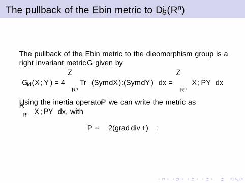
The pullback of the Ebin metric to DiffS(Rn)

The pullback of the Ebin metric to the diffeomorphism group is aright invariant metric G given by

GId(X ,Y ) = 4

∫Rn

Tr((Sym dX ).(Sym dY )

)dx =

∫Rn

⟨X ,PY

⟩dx

Using the inertia operator P we can write the metric as∫Rn

⟨X ,PY

⟩dx , with

P = −2(grad div +∆) .

The pullback of the general metric to DiffS(Rn)

We consider now a weak Riemannian metric on MetA(Rn) in itsgeneral form

GPg (h, k) =

∫M

g 02 (Pgh, k) vol(g) =

∫M

Tr(g−1.Pg (h).g−1.k) vol(g),

where Pg : Γ(S2T ∗M)→ Γ(S2T ∗M) is as described above. If theoperator P is equivariant for the action of DiffA(Rn) onMetA(Rn), then the induced pullback metric (Pullg )∗GP onDiffA(Rn) is right invariant:

GId(X ,Y ) = −4

∫Rn

∂j(Pg Sym dX )ij .Yidx (4)

Thus we we get the following formula for the corresponding inertiaoperator (PX )i =

∑j ∂j(Pg Sym dX )ij . Note that the pullback

metric (Pullg )∗GP on DiffA(Rn) is always of one order higher thenthe metric GP on MetA(Rn).

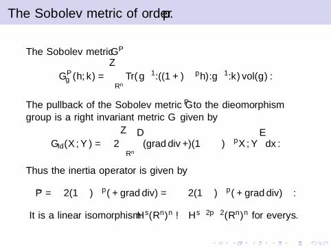
The Sobolev metric of order p.

The Sobolev metric GP

GPg (h, k) =

∫Rn

Tr(g−1.((1 + ∆)ph).g−1.k) vol(g) .

The pullback of the Sobolev metric GP to the diffeomorphismgroup is a right invariant metric G given by

GId(X ,Y ) = −2

∫Rn

⟨(grad div +∆)(1−∆)pX ,Y

⟩dx .

Thus the inertia operator is given by

P = −2(1−∆)p(∆ + grad div) = −2(1−∆)p(∆ + grad div) .

It is a linear isomorphism Hs(Rn)n → Hs−2p−2(Rn)n for every s.

Approximating the Euler equation of fluid mechanicson DiffH∞(Rn)

On the Lie algebra of VF XH∞(Rn) = H∞(Rn)n we consider aweak inner product of the form ‖v‖2

L =∫Rn〈Lv , v〉 dx where L is a

positive L2-symmetric (pseudo-) differential operator (inertiaoperator). Leads to a right invariant metric on DiffH∞(Rn) whosegeodesic equation is

∂tϕ = u ϕ, ∂tu = − ad>u u, where∫〈L(ad>u u), v〉 dx =

∫〈L(u),−[u, v ]〉 dx

Condsider the momentum m = L(v) of a vector field, so that〈v ,w〉L =

∫〈m,w〉dx . Then the geodesic equation is of the form:

∂tm = −(v · ∇)m − div(v)m −m · (Dv)t

∂tmi = −∑j

(vj∂xj mi + ∂xj vj ·mi + mj∂xi vj)

v = K ∗m, where K is the matrix-valued Green function of L.

Suppose, the time dependent vector field v integrates to a flow ϕvia

∂tϕ(x , t) = v(ϕ(x , t), t)

and we describe the momentum by a measure-valued 1-form

m =∑i

midxi ⊗ (dx1 ∧ · · · ∧ dxn)

so that ‖v‖2L =

∫(v , m) makes intrinsic sense. Then the geodesic

equation is equivalent to: m is invariant under the flow ϕ, that is,

m(·, t) = ϕ(·, t)∗m(·, 0),

whose infinitesimal version is the following, using the Lie derivative:

∂tm(·, t) = −Lv(·,t)m(·, t).

Because of this invariance, if a geodesic begins with momentum ofcompact support, its momentum will always have compactsupport; and if it begins with momentum which, along with all itsderivatives, has ‘rapid’ decay at infinity, that is it is in O(‖x‖−n)for every n, this too will persist, because DiffS(Rn) ⊂ DiffH∞(Rn)is a normal subgroup.Moreover this invariance gives us a Lagrangian form of EPDiff:

∂tϕ(x , t) =

∫Kϕ(·,t)(x , y)(ϕ(y , t)∗m(y , 0))

= Kϕ(·,t) ∗ (ϕ(·, t)∗m(·, 0))

where Kϕ(x , y) = K (ϕ(x), ϕ(y))

Aim of this talk: Solutions of Euler’s equation are limits ofsolutions of equations in the EPDiff class with the operator:

Lε,η = (I − η2

p 4)p (I − 1ε2∇ div), for any ε > 0, η ≥ 0.

All solutions of Euler’s equation are limits of solutions of thesemuch more regular EPDiff equations and give a bound on theirrate of convergence. In fact, so long as p > n/2 + 1, these EPDiffequations have a well-posed initial value problem with uniquesolutions for all time. Moreover, although L0,η does not makesense, the analog of its Green’s function K0,η does make sense asdo the geodesic equations in momentum form. These are, in fact,geodesic equations on the group of volume preservingdiffeomorphisms SDiff and become Euler’s equation for η = 0. Animportant point is that so long as η > 0, the equations havesoliton solutions (called vortons) in which the momentum is a sumof delta functions.

Relation to Euler’s equ. Oseledetz 1988

We use the kernel

Kij(x) = δijδ0(x) + ∂xi∂xj H

where H is the Green’s function of −∆. But K now has a rathersubstantial pole at the origin. If Vn = Vol(Sn−1),

H(x) =

1

(n−2)Vn(1/|x |n−2) if n > 2,

1V2

log(1/|x |) if n = 2

so that, as a function

(M0)ij(x) := ∂xi∂xj H(x) =1

Vn·

nxixj − δij |x |2

|x |n+2, if x 6= 0.

Convolution with any (M0)ij is still a Calderon-Zygmund singularintegral operator defined by the limit as ε→ 0 of its value outsidean ε-ball, so it is reasonably well behaved. As a distribution thereis another term:

∂xi∂xj Hdistribution

= (M0)ij −1

nδijδ0

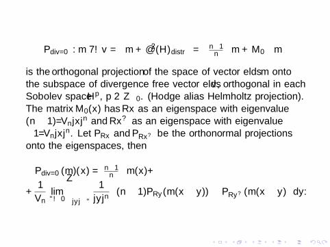
Pdiv=0 : m 7→ v =(m + ∂2(H)distr

)=(n−1n ·m + M0 ∗m

)is the orthogonal projection of the space of vector fields m ontothe subspace of divergence free vector fields v , orthogonal in eachSobolev space Hp, p ∈ Z≥0. (Hodge alias Helmholtz projection).The matrix M0(x) has Rx as an eigenspace with eigenvalue(n − 1)/Vn|x |n and Rx⊥ as an eigenspace with eigenvalue−1/Vn|x |n. Let PRx and PRx⊥ be the orthonormal projectionsonto the eigenspaces, then

Pdiv=0(m)(x) = n−1n ·m(x)+

+1

Vn· limε→0

∫|y |≥ε

1

|y |n((n − 1)PRy (m(x − y))− PRy⊥(m(x − y)

)dy .

With this K , EPDiff in the variables (v ,m) is the Euler equation inv with pressure a function of (v ,m). Oseledets’s form for Euler:

v = Pdiv=0(m)

∂tm = −(v · ∇)m −m · (Dv)t

Let m =∑

i midxi be the 1-form associated to m. Since div v = 0,we can use m instead of

∑i midxi ⊗ dx1 ∧ . . . dxn. Integrated form:

∂tϕ = Pdiv=0(m) ϕm(·, t) = ϕ(·, t)∗m(·, 0)

This uses the variables v ,m instead of v and pressure.Advantage: m, like vorticity, is constant when transported by theflow. m determines the vorticity the 2-form ω = d(

∑i vidxi ),

because v and m differ by a gradient, so ω = dm also. Thus:vorticity is constant along flows follows from the same fact formomentum 1-form m.

However, these equ. are not part of the true EPDiff frameworkbecause the operator K = Pdiv=0 is not invertible and there is nocorresponding differential operator L.In fact, v does not determine m as we have rewritten Euler’sequation using extra non-unique variables m, albeit ones whichobey a conservation law so they may be viewed simply as extraparameters.

Approximationg Euler by EPDiff

Replace the Green’s function H of −∆ by the Green’s function Hε

of the positive ε2I −4 for ε > 0 (whose dimension is length−1).The Green’s function is be given explicitly using the ‘K’ Besselfunction via the formula

Hε(x) = cnεn−2|εx |1−n/2Kn/2−1(|εx |)

for a suitable constant cn independent of ε. Then we get themodified kernel

(Kε)ij = δijδ0 + (∂xi∂xj Hε)distr

This has exactly the same highest order pole at the origin as K didand the second derivative is again a Calderon-Zygmund singularintegral operator minus the same delta function. The maindifference is that this kernel has exponential decay at infinity, notpolynomial decay. By weakening the requirement that the velocitybe divergence free, the resulting integro-differential equationbehaves much more locally, more like a hyperbolic equation ratherthan a parabolic one.

The corresponding inverse is the differential operator

Lε = I − 1ε2∇ div

v = Kε ∗m, m = Lε(v)

‖v‖2Lε =

∫〈v , v〉+ div(v). div(v)dx

Geodesic equation:

∂t(vi ) = (Kε)ij ∗ ∂t(mj)

= −(Kε)ij ∗ (vkvj ,k)− vi div(v)− 12 (Kε)ij ∗

(|v(x)|2 + ( div(v)

ε )2),j

Curiously though, the parameter ε can be scaled away. That is, ifv(x , t),m(x , t) is a solution of EPDiff for the kernel K1, thenv(εx , εt),m(εx , εt) is a solution of EPDiff for Kε.

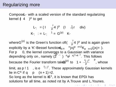
Regularizing more

Compose Lε with a scaled version of the standard regularizingkernel (I −4)p to get

Lε,η = (I − η2

p 4)p (I − 1ε2∇ div)

Kε,η : = Lε,η−1 = G (p)

η ∗ Kε

where G(p)η is the Green’s function of (I − η2

p 4)p and is again given

explicitly by a ‘K’-Bessel function dp,nη−n|x |p−n/2Kp−n/2(|x |/η).

For p 0, the kernel converges to a Gaussian with variancedepending only on η, namely (2

√πη)−ne−|x |

2/4η2. This follows

because the Fourier transform takes G(p)η to

(1 + η2|ξ|2

p

)−p, whose

limit, as p →∞, is e−η2|ξ|2 . These approximately Gaussian kernels

lie in Cq if q ≤ p − (n + 1)/2.So long as the kernel is in C 1, it is known that EPDiff hassolutions for all time, as noted first by A.Trouve and L.Younes.

Theorem

Let F (x) = f (|x |) be any integrable C 2 radial function on Rn.Assume n ≥ 3. Define:

HF (x) =

∫Rn

min(

1|x |n−2 ,

1|y |n−2

)F (y)dy

=1

|x |n−2

∫|y |≤|x |

F (y)dy +

∫|y |≥|x |

F (y)

|y |n−2dy

Then HF is the convolution of F with 1|x |n−2 , is in C 4 and:

∂i (HF )(x) = −(n − 2)xi|x |n

∫|y |≤|x |

F (y)dy

∂i∂j(HF )(x) = (n − 2)

(nxixj − δij |x |2

|x |n+2

∫|y |≤|x |

F (y)dy − Vnxixj|x |2

F (x)

)

If n = 2, the same holds if you replace 1/|x |n−2 by log(1/|x |) andomit the factors (n − 2) in the derivatives.

no L K0,0 = Pdiv=0 = δijδ0 + (∂i∂jH)distr

no L K0,η = G(p)η ∗ Pdiv=0 – see above

Lε,0 = I − 1ε2∇ div Kε,0 = δijδ0 + ∂i∂jHε

Lε,η =(

I − η2

p 4)p Kε,η = δijG

(p)η + ∂i∂j(G

(p)η ∗ Hε)

(I − 1

ε2∇ div)

Theorem: Let ε ≥ 0, η > 0, p ≥ (n + 3)/2 and K = Kε,η be thecorresponding kernel. For any vector-valued distribution m0 whosecomponents are finite signed measures, consider the Lagrangianequation for a time varying C 1-diffeomorphism ϕ(·, t) withϕ(x , 0) ≡ x:

∂tϕ(x , t) =

∫K (ϕ(x , t)− ϕ(y , t))(Dϕ(y , t))−1,>m0(y)dy .

Here Dϕ is the spatial derivative of ϕ. This equation has a uniquesolution for all time t.

Proof: The Eulerian velocity at ϕ is:

Vϕ(x) =

∫K (x − ϕ(y))(Dϕ(y))−1,>m0(y)dy

and Wϕ(x) = Vϕ(ϕ(x)) is the velocity in ‘material’ coordinates.Note that because of our assumption on m0, if ϕ is aC 1-diffeomorphism, then Vϕ and Wϕ are C 1 vector fields on Rn; infact, they are as differentiable as K is, for suitably decaying m.The equation can be viewed as a the flow equation for the vectorfield ϕ 7→Wϕ on the union of the open sets

Uc =ϕ ∈ C 1(Rn)n : ‖ Id−ϕ‖C1 < 1/c , det(Dϕ) > c

,

where c > 0. The union of all Uc is the group DiffC1b(Rn) of all

C 1-diffeomorphisms which, together with their inverses, differ fromthe identity by a function in C 1(Rn)n with bounded C 1-norm. Weclaim this vector field is locally Lipschitz on each Uc :

‖Wϕ1 −Wϕ2‖C1 ≤ C .‖ϕ1 − ϕ2‖C1

where C depends only on c : Use that K is uniformly continuousand use ‖Dϕ−1‖ ≤ ‖Dϕ‖n−1/| det(Dϕ)|.

As a result we can integrate the vector field for short times inDiffC1

b(Rn). But since (Dϕ(y , t))−1,>m0(y) is then again a signed

finite Rn-valued measure,∫Vϕ(·,t)(x)(Dϕ(y , t))−1,>m0(y)dx = ‖Vϕ(·,t)‖Lε,η

is actually finite for each t. Using the fact that in EPDiff theLε,η-energy ‖Vϕ(·,t)‖Lε,η of the Lε,η-geodesic is constant in t, weget a bound on the norm ‖Vϕ(·,t)‖Hp , depending of course on ηbut independent of t, hence a bound on ‖Vϕ(·,t)‖C1 . Thus‖ϕ(·, t)‖C0 grows at most linearly in t. But∂tDϕ = DWϕ = DVϕ ·Dϕ which shows us that Dϕ grows at mostexponentially in t. Hence det Dϕ can shrink at worst exponentiallytowards zero, because ∂t det(Dϕ) = Tr(Adj(Dϕ).∂tDϕ). Thus forall finite t, the solution ϕ(·, t) stays in a bounded subset of ourBanach space and the ODE can continue to be solved. QED.

Lemma: If η ≥ 0 and ε > 0 are bounded above, then the norm

‖v‖2k,ε,η =

∑|α|≤k

∫〈DαLε,ηv ,Dαv〉dx

is bounded above and below by the metric, with constantsindependent of ε and η:

‖v‖2Hk + 1

ε2 ‖div(v)‖2Hk +

∑k+1≤|α|≤k+p

η2(|α|−k)

∫|Dαv |2+ 1

ε2 |Dαdiv(v)|2

Main estimate: Assume k is sufficiently large, for instancek ≥ (n + 2p + 4) works, then the velocity field of a solutionsatisfies:

|∂t(‖v‖2

k,ε,η

)| ≤ C .‖v‖3

k,ε,η

where, so long ε and η are bounded above, the constant C isindependent of ε and η.

Theorem: Fix k , p, n with p > n/2 + 1, k ≥ n + 2p + 4 andassume (ε, η) ∈ [0,M]2 for some M > 0. Then there are constantst0,C such that for all initial v0 ∈ Hk+p+1, there is a uniquesolution vε,η(x , t) of EPDiff (including the limiting Euler case) fort ∈ [0, t0]. The solution vε,η(·, t) ∈ Hk+p+1 depends continuouslyon ε, η ∈ [0,M]2 and satisfies ‖vε,η(·, t)‖k,ε,η < C for all t ∈ [0, t0].Theorem: Take any k and M and any smooth initial velocityv(·, 0). Then there are constants t0,C such that Euler’s equationand (ε, 0)-EPDiff have solutions v0 and vε respectively fort ∈ [0, t0] and all ε < M and these satisfy:

‖v0(·, t)− vε(·, t)‖Hk ≤ Cε.

Theorem: Let ε > 0. Take any k and M and any smooth initialvelocity v(·, 0). Then there are constants t0,C such that(ε, 0)-EPDiff and (ε, η)-EPDiff have solutions v0 and vηrespectively for t ∈ [0, t0] and all ε, η < M and these satisfy:

‖v0(·, t)− vη(·, t)‖Hk ≤ Cη2.

Vortons: Soliton-like solutions via landmark theory

We have a C 1 kernel, so we can consider solutions in whichmomentum m is supported in a finite set P1, · · · ,PN, so thatthe components of the momentum field are given bymi (x) =

∑a maiδ(x − Pa). The support is called the set of

landmark points and in this case, EPDiff reduces to a set ofHamiltonian ODE’s based on the kernel K = Kε,η, ε ≥ 0, η > 0:

Energy E =∑a,b

maiKij(Pa − Pb)mjb

dPai

dt=∑b,j

Kij(Pa − Pb)mbj

dmai

dt= −

∑b,j ,k

∂xi Kjk(Pa − Pb)majmbk

where a, b enumerate the points and i , j , k the dimensions in Rn.These are essentially Roberts’ equations from 1972.

One landmark point

Its momentum must be constant hence so is its velocity. Thereforethe momentum moves uniformly in a straight line ` from −∞ to+∞.

−4 −3 −2 −1 0 1 2 3−2.5

−2

−1.5

−1

−0.5

0

0.5

1

1.5

2

2.5

Momentum is tranformed to vortex-like velocity field bykernel K0,ε

The dipole given by the kernel K0,η in dimension 2.

Streamlines and MatLab’s ‘coneplot’ to visualize the vector fieldgiven by the x1-derivative of the kernel K0,1 times the vector(1, 2, 0).

Two landmark points

0.0

50.0

5

0.1

0.1

0.2

50.2

5

0.25

0.5

0.5

0.5

11

1

11

22

2

2

44

4

4

8

8

8

|δ m|

ρ

0 0.5 1 1.5 2 2.5 3 3.5 4 4.5 5

2

4

6

8

10

12

14

Level sets of energy for the collision of two vortons with m = 0,η = 1, ω = 1. The coordinates are ρ = |δP| and |δm|, and thestate space is the double cover of the area above and right of theheavy black line, the two sheets being distinguished by the sign of〈δm, δP〉. The heavy black line which is the curve ρ · |δm| = ωwhere 〈δm, δP〉 = 0. Each level set is a geodesic. If they hit theblack line, they flip to the other sheet and retrace their path.Otherwise ρ goes to zero at one end of the geodesic.

Geodesics in the δP plane all starting at the point marked by an Xbut with m = m1 + m2 =const. along the y -axis varying from 0 to10. Here η = 1, the initial point is (5, 0) and the initial momentumis (−3, .5). Note how the two vortons repel each other on somegeodesics and attract on others. A blow up shows the spiralingbehavior as they collapse towards each other.

Robust Infinite Dimensional Riemannian manifolds,Sobolev Metrics on Diffeomorphism Groups, and theDerived Geometry of Shape Spaces

Based on: [Mario Micheli, Peter W. Michor, David Mumford: Sobolev

Metrics on Diffeomorphism Groups and the Derived Geometry of Spaces

of Submanifolds. Izvestiya: Mathematics 77:3 (2013), 541-570.]

Recall: Geodesics of a right invariant metric

Let γ = 〈 , 〉 : g× g→ R be a positive definite bounded weakinner product; so γ : g→ g∗ is injective. Then

γx(ξ, η) = 〈T (µx−1

) · ξ,T (µx−1

) · η)〉 = 〈κ(ξ), κ(η)〉

is a right invariant weak Riemannian metric on G .Let g : [a, b]→ G be a smooth curve. In terms of its rightlogarithmic derivative u : [a, b]→ g,u(t) := g∗κ(∂t) = Tg(t)(µg(t)−1

) · g ′(t) = g ′(t).g(t)−1, thegeodesic equation is

γ(ut) = − ad(u)∗γ(u)

Condition for the existence of the geodesic equation:

X 7→ γ−1(ad(X )∗γ(X ))

is bounded quadratic g → g .

We treated in detail a situation where ad(X )∗γ(X ) ∈ γ(g) for allX ∈ g , but the more general [Arnold 1966] conditionad(X )∗γ(Y ) ∈ γ(g) for all X ,Y ∈ g does not hold.[M. Bauer, M. Bruveris, P. Michor: The homogeneous Sobolevmetric of order one on diffeomorphism groups on the real line.Journal of Nonlinear Science. doi:10.1007/s00332-014-9204-y.arXiv:1209.2836]

Note also the geodesic equation for the momentum α = γ(u):

αt = − ad(γ−1(α))∗ α = − ad(α])∗α. = − ad(u)∗ α.

The covariant derivative for a right invariant metric

The right trivialization, or framing, (πG , κ) : TG → G × g inducesthe isomorphism R : C∞(G , g)→ X(G ), given byR(X )(x) := RX (x) := Te(µx) · X (x), for X ∈ C∞(G , g) andx ∈ G . Here X(G ) := Γ(TG ) denote the Lie algebra of all vectorfields. For the Lie bracket and the Riemannian metric we have

[RX ,RY ] = R(−[X ,Y ]g + dY · RX − dX · RY ),

R−1[RX ,RY ] = −[X ,Y ]g + RX (Y )− RY (X ),

γx(RX (x),RY (x)) = γ(X (x),Y (x)) , x ∈ G .

In the sequel we shall compute in C∞(G , g) instead of X(G ). Inparticular, we shall use the convention

∇XY := R−1(∇RXRY ) for X ,Y ∈ C∞(G , g).

to express the Levi-Civita covariant derivative.

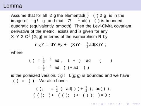
Lemma

Assume that for all ξ ∈ g the element ad(ξ)∗γ(ξ) ∈ g∗ is in theimage of γ : g→ g∗ and that ξ 7→ γ−1 ad(ξ)∗γ(ξ) is boundedquadratic (equivalently, smooth). Then the Levi-Civita covariantderivative of the metric γ exists and is given for anyX ,Y ∈ C∞(G , g) in terms of the isomorphism R by

∇XY = dY .RX + ρ(X )Y − 12 ad(X )Y ,

where

ρ(ξ)η = 14 γ−1(

ad∗ξ+η γ(ξ + η)− ad∗ξ−η γ(ξ − η))

= 12 γ−1(

ad∗ξ γ(η) + ad∗η γ(ξ))

is the polarized version. ρ : g→ L(g, g) is bounded and we haveρ(ξ)η = ρ(η)ξ. We also have:

γ(ρ(ξ)η, ζ

)= 1

2γ(ξ, ad(η)ζ) + 12γ(η, ad(ξ)ζ) ,

γ(ρ(ξ)η, ζ) + γ(ρ(η)ζ, ξ) + γ(ρ(ζ)ξ, ξ) = 0 .

The curvature

For X ,Y ∈ C∞(G , g) we have

[RX , ad(Y )] = ad(RX (Y )) and [RX , ρ(Y )] = ρ(RX (Y )).

The Riemannian curvature is then computed by

R(X ,Y ) = [∇X ,∇Y ]−∇−[X ,Y ]g+RX (Y )−RY (X )

= [RX + ρX − 12 adX ,RY + ρY − 1

2 adY ]

− R(−[X ,Y ]g + RX (Y )− RY (X ))

− ρ(−[X ,Y ]g + RX (Y )− RY (X ))

+ 12 ad(−[X ,Y ]g + RX (Y )− RY (X ))

= [ρX , ρY ] + ρ[X ,Y ]g −12 [ρX , adY ] + 1

2 [ρY , adX ]− 14 ad[X ,Y ]g

which visibly is a tensor field.

Sectional Curvature. For a linear 2-dim. subspace P ⊆ g spannedby X ,Y ∈ g, the sectional curvature is defined as:

k(P) = −γ(R(X ,Y )X ,Y

)‖X‖2

γ‖Y ‖2γ − γ(X ,Y )2

.

For the numerator we get:

γ(R(X ,Y )X ,Y

)= γ(ρXX , ρY Y )− ‖ρXY ‖2

γ + 34‖[X ,Y ]‖2

γ

− 12γ(X , [Y , [X ,Y ]]) + 1

2γ(Y , [X , [X ,Y ]]).

= γ(ρXX , ρY Y )− ‖ρXY ‖2γ + 3

4‖[X ,Y ]‖2γ

− γ(ρXY , [X ,Y ]]) + γ(Y , [X , [X ,Y ]]) .

If the adjoint ad(X )> : g→ g exists, this is easily seen to coincidewith Arnold’s original formula [Arnold1966],

γ(R(X ,Y )X ,Y ) = −14‖ ad(X )>Y + ad(Y )>X‖2

γ

+ γ(ad(X )>X , ad(Y )>Y )

+ 12γ(ad(X )>Y − ad(Y )>X , ad(X )Y ) + 3

4‖[X ,Y ]‖2γ .

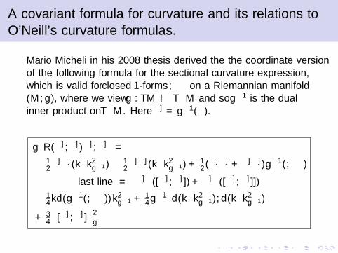
A covariant formula for curvature and its relations toO’Neill’s curvature formulas.

Mario Micheli in his 2008 thesis derived the the coordinate versionof the following formula for the sectional curvature expression,which is valid for closed 1-forms α, β on a Riemannian manifold(M, g), where we view g : TM → T ∗M and so g−1 is the dualinner product on T ∗M. Here α] = g−1(α).

g(R(α], β])α], β]

)=

− 12α

]α](‖β‖2g−1)− 1

2β]β](‖α‖2

g−1) + 12 (α]β] + β]α])g−1(α, β)(

last line = −α]β([α], β]]) + β]α([α], β]]]))

− 14‖d(g−1(α, β))‖2

g−1 + 14 g−1

(d(‖α‖2

g−1), d(‖β‖2g−1)

)+ 3

4

∥∥[α], β]]∥∥2

g

Mario’s formula in coordinates

Assume that α = αidx i , β = βidx i where the coefficients αi , βi areconstants, hence α, β are closed.Then α] = g ijαi∂j , β

] = g ijβi∂j and we have:

4g(R(α], β])β], α]

)= (αiβk − αkβi ) · (αjβl − αlβj)·

·(

2g is(g jtgkl,t ),s − 1

2 g ij,sg stgkl

,t − 3g isgkp,s gpqg jtg lq

,t

)

Covariant curvature and O’Neill’s formula, finite dim.

Let p : (E , gE )→ (B, gB) be a Riemannian submersion:For b ∈ B and x ∈ Eb := p−1(b) the gE -orthogonal splitting

TxE = Tx(Ep(x))⊕ Tx(Ep(x))⊥,gE =: Tx(Ep(x))⊕ Horx(p).

Txp : (Horx(p), gE )→ (TbB, gB)

is an isometry. A vector field X ∈ X(E ) is decomposed asX = X hor + X ver into horizontal and vertical parts. Each vectorfield ξ ∈ X(B) can be uniquely lifted to a smooth horizontal fieldξhor ∈ Γ(Hor(p)) ⊂ X(E ).

O’Neill’s formula says that for any two horizontal vector fieldsX ,Y on E and any x ∈ E , the sectional curvatures of E and B arerelated by:

gBp(x)(RB(p∗(Xx), p∗(Yx))p∗(Yx), p∗(Xx))

= gEx (RE (Xx ,Yx)Yx ,Xx) + 3

4‖[X ,Y ]ver‖2x .

Comparing Mario’s formula on E and B gives an immediate proofof this fact. Namely: If α ∈ Ω1(B), then the vector field (p∗α)] ishorizontal and we have Tp (p∗α)] = α] p. Therefore (p∗α)]

equals the horizontal lift (α])hor. For each x ∈ E the mapping(Txp)∗ : (T ∗p(x)B, g−1

B )→ (T ∗x E , g−1E ) is an isometry. We also use:

‖[(p∗α)], (p∗β)]]hor‖2gE

= p∗‖[α], β]]‖2gB

Requirements for infinite dimensional manifolds

Let (M, g) be a weak Riemannian manifold, modeled onconvenient locally convex vector spaces: Weak: gx : TxM → T ∗x Mis only injective. The image g(TM) ⊂ T ∗M is called the smoothcotangent bundle associated to g . Now Ω1

g (M) := Γ(g(TM)) and

α] = g−1α ∈ X(M),X [ = gX are as above.d : Ω1

g (M)→ Ω2(M) = Γ(L2skew(TM;R)).

Existence of the Levi-Civita covariant derivative is equivalent to:The metric itself admits symmetric gradients with respect to itself.Locally: If M is c∞-open in a convenient vector space VM . Then:

Dx ,Xgx(X ,Y ) = gx(X , grad1 g(x)(X ,Y ))

= gx(grad2 g(x)(X ,X ),Y )

where grad1 g , sym grad2 g : M × VM × VM → VM given by(x ,X ) 7→ grad1,2 g(x)(X ,X ) are smooth and quadratic in X ∈ VM .Then the rest of the derivation of Mario’s formula goes throughand the final formula for curvature holds in both the finite andinfinite dimensional cases.

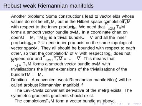
Robust weak Riemannian manifolds

Another problem: Some constructions lead to vector fields whosevalues do not lie in TxM, but in the Hilbert space completion TxMwith respect to the inner product gx . We need that

⋃x∈M TxM

forms a smooth vector bundle over M. In a coordinate chart onopen U ⊂ M, TM|U is a trivial bundle U × V and all the innerproducts gx , x ∈ U define inner products on the same topologicalvector space V . They all should be bounded with respect to eachother, so that the completion V of V with respect to gx does notdepend on x and

⋃x∈U TxM ∼= U × V . This means that⋃

x∈M TxM forms a smooth vector bundle over M withtrivialisations the linear extensions of the trivialisations of thebundle TM → M.Definition A convenient weak Riemannian manifold (M, g) will becalled a robust Riemannian manifold if• The Levi-Civita convariant derivative of the metric g exists: Thesymmetric gradients gradients should exist.• The completions TxM form a vector bundle as above.

Covariant curvature and O’Neill’s formula

Some subtle considerations lead to:Theorem. Let p : (E , gE )→ (B, gB) be a Riemann submersionbetween infinite dimensional robust Riemann manifolds. Then for1-forms α, β ∈ Ω1

gB(B) O’Neill’s formula holds in the form:

gB(RB(α], β])β], α]

)= gE

(RE ((p∗α)], (p∗β)])(p∗β)], (p∗α)]

)+ 3

4‖[(p∗α)], (p∗β)]]ver‖2gE

Semilocal version of Mario’s formula, force, and stress

Let (M, g) be a robust Riemannian manifold, x ∈ M,α, β ∈ gx(TxM). Assume we are given local smooth vector fieldsXα and Xβ such that:

1. Xα(x) = α](x), Xβ(x) = β](x),

2. Then α] − Xα is zero at x hence has a well defined derivativeDx(α] − Xα) lying in Hom(TxM,TxM). For a vector field Ywe have Dx(α]−Xα).Yx = [Y , α]−Xα](x) = LY (α]−Xα)|x .The same holds for β.

3. LXα(α) = LXα(β) = LXβ (α) = LXβ (β) = 0,

4. [Xα,Xβ] = 0.

Locally constant 1-forms and vector fields will do. We then define:

F(α, β) : = 12 d(g−1(α, β)), a 1-form on M called the force,

D(α, β)(x) : = Dx(β] − Xβ).α](x)

= d(β] − Xβ).α](x), ∈ TxM called the stress.

=⇒ D(α, β)(x)−D(β, α)(x) = [α], β]](x)

Then in the notation above:

g(R(α], β])β], α]

)(x) = R11 + R12 + R2 + R3

R11 = 12

(L2Xα(g−1)(β, β)− 2LXαLXβ (g−1)(α, β)

+ L2Xβ

(g−1)(α, α))

(x)

R12 = 〈F(α, α),D(β, β)〉+ 〈F(β, β),D(α, α)〉− 〈F(α, β),D(α, β) +D(β, α)〉

R2 =(‖F(α, β)‖2

g−1 −⟨F(α, α)),F(β, β)

⟩g−1

)(x)

R3 = −34‖D(α, β)−D(β, α)‖2

gx

Diffeomorphism groups

Let N be a manifold. We consider the following regular Lie groups:

Diff(N), the group of all diffeomorphisms of N if N is compact.Diffc(N), the group of diffeomorphisms with compact support.

If (N, g) is a Riemannian manifold of bounded geometry, we alsomay consider:

DiffS(N), the group of all diffeos which fall rapidly to the identity.DiffH∞(N), the group of all diffeos which are modelled on thespace ΓH∞(TM), the intersection of all Sobolev spaces of vectorfields.

The Lie algebras are the spaces XA(N) of vector fields, whereA ∈ C∞c ,S,H∞, with the negative of the usual bracket as Liebracket.

Riemann metrics on Diff(N).

The concept of robust Riemannian manifolds, and also thereproducing Hilbert space approach in Chapter 12 of [Younes 2010]leads to:We construct a right invariant weak Riemannian metric byassuming that we have a Hilbert space H together with twobounded injective linear mappings

XS(N) = ΓS(TN)j1−−→ H j2−−→ ΓC2

b(TN) (1)

where ΓC2b(TN) is the Banach space of all C 2 vector fields X on N

which are globally bounded together with ∇gX and ∇g∇gX withrespect to g , such that j2 j1 : ΓS(TN)→ ΓC2

b(TN) is the

canonical embedding. We also assume that j1 has dense image.

Dualizing the Banach spaces in equation (1) and using thecanonical isomorphisms between H and its dual H′ – which we callL and K , we get the diagram:

ΓS(TN) _j1

ΓS′(T ∗N)

H _j2

L // H′?

j ′1

OO

Koo

ΓC2b(TN) ΓM2(T ∗N)

?

j ′2

OO

Here ΓS′(T ∗N), the space of 1-co-currents, is the dual of thespace of smooth vector fields ΓS(TN) = XS(N). It contains thespace ΓS(T ∗N ⊗ vol(N)) of smooth measure valued cotangentvectors on N, and also the bigger subspace of second derivatives offinite measure valued 1-forms on N, written as ΓM2(T ∗N) which ispart of the dual of ΓC2

b(TN). In what follows, we will have many

momentum variables with values in these spaces.

The restriction of L to XS(N) via j1 gives us a positive definiteweak inner product on XS(N) which may be defined by adistribution valued kernel – which we also write as L:

〈 , 〉L : XS(N)× XS(N)→ R, defined by

〈X ,Y 〉L = 〈j1X , j1Y 〉H =

∫∫N×N

(X (y1)⊗ Y (y2), L(y1, y2)),

where L ∈ ΓS′(pr∗1(T ∗N)⊗ pr∗2(T ∗N))

Extending this weak inner product right invariantly over DiffS(N),we get a robust weak Riemannian manifold.Given an operator L with appropriate properties we can reconstructthe Hilbert space H with the two bounded injective mappings j1, j2.

In the case (called the standard case below) that N = Rn and that

〈X ,Y 〉L =

∫Rn

〈(1− A∆)lX ,Y 〉 dx

we have

L(x , y) =( 1

(2π)n

∫ξ∈Rn

e i〈ξ,x−y〉(1 + A|ξ|2)ldξ)

n∑i=1

(dui |x ⊗ dx)⊗ (dui |y ⊗ dy)

where dξ, dx and dy denote Lebesque measure, and where (ui ) arelinear coordinates on Rn. Here H is the space of Sobolev H l vectorfields on N.

Construction of the reproducing kernel K

The inverse map K of L is given by a C 2 tensor, the reproducingkernel. Namely, ΓM2(T ∗N) contains the measures supported atone point x defined by an element αx ∈ T ∗x N. Then j2(K (j ′2(αx)))is given by a C 2 vector field Kαx on N which satisfies:

〈Kαx ,X 〉H = αx(j2X )(x) for all X ∈ H, αx ∈ T ∗x N. (*)

The map αx 7→ Kαx is weakly C 2b , thus by [KM97, theorem 12.8]

strongly Lip1. Since evy K : T ∗x N 3 αx 7→ Kαx (y) ∈ TyN is linearwe get a corresponding elementK (x , y) ∈ L(T ∗x N,TyN) = TxN ⊗ TyN withK (y , x)(αx) = Kαx (y).Using (*) twice we have (omitting j2)

βy .K (y , x)(αx) = 〈K ( , x)(αx),K ( , y)(βy )〉H = αx .K (x , y)(βy )

so that:I K (x , y)> = K (y , x) : T ∗y N → TxN,I K ∈ ΓC2

b(pr1

∗ TN ⊗ pr∗2 TN).

Moreover the operator K defined directly by integration

K : ΓM2(T ∗N)→ ΓS(TN)

K (α)(y2) =

∫y1∈N

(K (y1, y2), α(y1)).

is the same as the inverse K to L.We will sometimes use the abbreviations 〈α|K |, |K |β〉 and 〈α|K |β〉for the contraction of the vector values of K in its first and secondvariable against 1-forms α and β. Often these are measure valued1-forms so after contracting, there remains a measure in thatvariable which can be integrated.

Thus the C 2 tensor K determines L and hence H and hence thewhole metric on DiffS(N). It is tempting to start with the tensorK , assuming it is symmetric and positive definite in a suitablesense. But rather subtle conditions on K are required in order thatits inverse L is defined on all infinitely differentiable vector fields.For example, if N = R, the Gaussian kernel K (x , y) = e−|x−y |

2

does not give such an L.In the standard case we have

K (x , y) = Kl(x − y)n∑

i=1

∂

∂x i⊗ ∂

∂y i,

Kl(x) =1

(2π)n

∫ξ∈Rn

e i〈ξ,x〉

(1 + A|ξ|2)ldξ

where Kl is given by a classical Bessel function of differentiabilityclass C 2l .

The zero compressibility limit

The case originally studied by Arnold – the L2 metric on volumepreserving diffeomorphisms – is not included in the family ofmetrics described above. But they do include metrics which havethis case as a limit. Taking N = Rn and starting with the standardSobolev metric, we can add a divergence term with a coefficient B:

〈X ,Y 〉L =

∫Rn

(〈(1− A∆)lX ,Y 〉+ B.div(X )div(Y )

)dx

Note that as B approaches ∞, the geodesics will tend to lie on thecosets with respect to the subgroup of volume preservingdiffeomorphisms. And when, in addition, A approaches zero, weget the simple L2 metric used by Arnold. This suggests that, as inthe so-called ‘zero-viscosity limit’, we should be able to constructgeodesics in Arnold’s metric, i.e. solutions of Euler’s equation, aslimits of geodesics for this larger family of metrics on the full group.

The resulting kernels L and K are no longer diagonal. To L, wemust add

Bn∑

i=1

n∑j=1

( 1

(2π)n

∫ξ∈Rn

e i〈ξ,x−y〉ξi .ξjdξ)

(dui |x⊗dx)⊗(duj |y⊗dy).

It can be checked that the corresponding kernel K will have theform

K (x , y) = K0(x−y)n∑

i=1

∂

∂x i⊗ ∂

∂y i+

n∑i=1

n∑j=1

(KB),ij(x−y)∂

∂x i⊗ ∂

∂y j

where K0 is the kernel as above for the standard norm of order land KB is a second radially symmetric kernel on Rn depending onB.

The geodesic equation on DiffS(N)

According to [Arnold 1966], slightly generalized as explainedabove: Let ϕ : [a, b]→ DiffS(N) be a smooth curve. In terms ofits right logarithmic derivative u : [a, b]→ XS(N),u(t) := ϕ∗κ(∂t) = Tϕ(t)(µϕ(t)−1

) · ϕ′(t) = ϕ′(t) ϕ(t)−1, thegeodesic equation is

L(ut) = − ad(u)∗L(u)

Condition for the existence of the geodesic equation:

X 7→ K (ad(X )∗L(X ))

is bounded quadratic XS(N)→ XS(N).

The Lie algebra of DiffS(N) is the space XS(N) of all rapidlydecreasing smooth vector fields with Lie bracket the negative ofthe usual Lie bracket adX Y = −[X ,Y ].

Using Lie derivatives, the computation of ad∗X is especially simple.Namely, for any section ω of T ∗N ⊗ vol and vector fieldsξ, η ∈ XS(N), we have:∫

N(ω, [ξ, η]) =

∫N

(ω,Lξ(η)) = −∫N

(Lξ(ω), η),

hence ad∗ξ(ω) = +Lξ(ω).Thus the Hamiltonian version of the geodesic equation on thesmooth dual L(XS(N)) ⊂ ΓC2(T ∗N ⊗ vol) becomes

∂tα = − ad∗K(α) α = −LK(α)α,

or, keeping track of everything,

∂tϕ = u ϕ,∂tα = −Luα

u = K (α) = α], α = L(u) = u[.

(1)

One can also derive the geodesic equation from the conservedmomentum mapping J : T DiffS(N)→ XS(N)′ given byJ(g ,X ) = L Ad(g)>X where Ad(g)X = Tg X g−1. Thismeans that Ad(g(t))u(t) is conserved and 0 = ∂t Ad(g(t))u(t)leads quickly to the geodesic equation. It is remarkable that themomentum mapping exists if and only if (DiffS(N), 〈 , 〉L) is arobust weak Riemannian manifold.

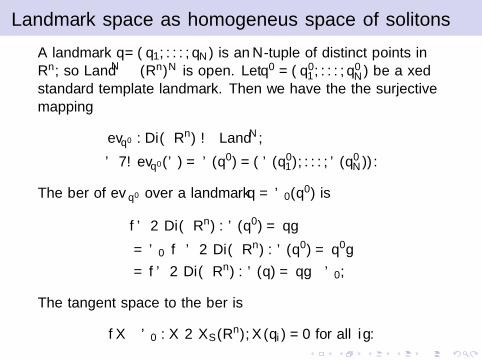
Landmark space as homogeneus space of solitons

A landmark q = (q1, . . . , qN) is an N-tuple of distinct points inRn; so LandN ⊂ (Rn)N is open. Let q0 = (q0

1 , . . . , q0N) be a fixed

standard template landmark. Then we have the the surjectivemapping

evq0 : Diff(Rn)→ LandN ,

ϕ 7→ evq0(ϕ) = ϕ(q0) = (ϕ(q01), . . . , ϕ(q0

N)).

The fiber of evq0 over a landmark q = ϕ0(q0) is

ϕ ∈ Diff(Rn) : ϕ(q0) = q= ϕ0 ϕ ∈ Diff(Rn) : ϕ(q0) = q0= ϕ ∈ Diff(Rn) : ϕ(q) = q ϕ0;

The tangent space to the fiber is

X ϕ0 : X ∈ XS(Rn),X (qi ) = 0 for all i.

A tangent vector Y ϕ0 ∈ Tϕ0 DiffS(Rn) is GLϕ0

-perpendicular tothe fiber over q if∫

Rn

〈LY ,X 〉 dx = 0 ∀X with X (q) = 0.

If we require Y to be smooth then Y = 0. So we assume thatLY =

∑i Pi .δqi , a distributional vector field with support in q.

Here Pi ∈ TqiRn. But then

Y (x) = L−1(∑

i

Pi .δqi

)=

∫Rn

K (x − y)∑i

Pi .δqi (y) dy

=∑i

K (x − qi ).Pi

Tϕ0(evq0).(Y ϕ0) = Y (qk)k =∑i

(K (qk − qi ).Pi )k

Now let us consider a tangent vector P = (Pk) ∈ Tq LandN . Itshorizontal lift with footpoint ϕ0 is Phor ϕ0 where the vector fieldPhor on Rn is given as follows: Let K−1(q)ki be the inverse of the(N × N)-matrix K (q)ij = K (qi − qj). Then

Phor(x) =∑i ,j

K (x − qi )K−1(q)ijPj

L(Phor(x)) =∑i ,j

δ(x − qi )K−1(q)ijPj

Note that Phor is a vector field of class H2l−1.

The Riemannian metric on LandN induced by the gL-metric onDiffS(Rn) is

gLq (P,Q) = GL

ϕ0(Phor,Qhor)

=

∫Rn

〈L(Phor),Qhor〉 dx

=

∫Rn

⟨∑i ,j

δ(x − qi )K−1(q)ijPj ,

∑k,l

K (x − qk)K−1(q)klQl

⟩dx

=∑i ,j ,k,l

K−1(q)ijK (qi − qk)K−1(q)kl〈Pj ,Ql〉

gLq (P,Q) =

∑k,l

K−1(q)kl〈Pk ,Ql〉. (1)

The geodesic equation in vector form is:

qn =

− 1

2

∑k,i ,j ,l

K−1(q)ki grad K (qi − qj)(K (q)in − K (q)jn)

K−1(q)jl〈qk , ql〉

+∑k,i

K−1(q)ki

⟨grad K (qi − qn), qi − qn

⟩qk

The geodesic equation on T ∗LandN(Rn)

.The cotangent bundleT ∗LandN(Rn) = LandN(Rn)× ((Rn)N)∗ 3 (q, α). We shall treatRn like scalars; 〈 , 〉 is always the standard inner product on Rn.The metric looks like

(gL)−1q (α, β) =

∑i ,j

K (q)ij〈αi , βj〉,

K (q)ij = K (qi − qj).

The energy function

E (q, α) = 12 (gL)−1

q (α, α) = 12

∑i ,j

K (q)ij〈αi , αj〉

and its Hamiltonian vector field (using Rn-valued derivatives tosave notation)

HE (q, α) =N∑

i ,k=1

(K (qk − qi )αi

∂

∂qk

+ grad K (qi − qk)〈αi , αk〉∂

∂αk

).

So the geodesic equation is the flow of this vector field:

qk =∑i

K (qi − qk)αi

αk = −∑i

grad K (qi − qk)〈αi , αk〉

Stress and Force

α]k =∑i

K (qk − qi )αi , α] =∑i ,k

K (qk − qi )〈αi ,∂∂qk〉

D(α, β) : =∑i ,j

dK (qi − qj)(α]i − α]j )⟨βj ,

∂

∂qi

⟩, the stress.

D(α, β)−D(β, α) = (Dα]β])− Dβ]α

] = [α], β]], Lie bracket.

Fi (α, β) =1

2

∑k

grad K (qi − qk)(〈αi , βk〉+ 〈βi , αk〉)

F(α, β) : =∑i

〈Fi (α, β), dqi 〉 =1

2d g−1(α, β) the force.

The geodesic equation on T ∗ LandN(Rn) then becomes

q = α]

α = −F(α, α)

Curvature via the cotangent bundle

From the semilocal version of Mario’s formula for the sectionalcurvature expression for constant 1-forms α, β on landmark space,where α]k =

∑i K (qk − qi )αi , we get directly:

gL(R(α], β])α], β]

)=

=⟨D(α, β) +D(β, α),F(α, β)

⟩−⟨D(α, α),F(β, β)

⟩−⟨D(β, β),F(α, α)

⟩− 1

2

∑i ,j

(d2K (qi − qj)(β]i − β

]j , β

]i − β

]j )〈αi , αj〉

− 2d2K (qi − qj)(β]i − β]j , α

]i − α

]j )〈βi , αj〉

+ d2K (qi − qj)(α]i − α]j , α

]i − α

]j )〈βi , βj〉

)− ‖F(α, β)‖2

g−1 + g−1(F(α, α),F(β, β)

).

+ 34‖[α

], β]]‖2g

Bundle of embeddings over the differentiable Chow variety.

Let M be a compact connected manifold with dim(M) < dim(N).The smooth manifold Emb(M,N) of all embeddings M → N is thetotal space of a smooth principal bundle with structure groupDiff(M) acting freely by composition from the right hand side.

The quotient manifold B(M,N) can be viewed as the space of allsubmanifolds of N of diffeomorphism type M; we call it thedifferentiable Chow manifold or the non-linear Grassmannian.

B(M,N) is a smooth manifold with charts centered atF ∈ B(M,N) diffeomorphic to open subsets of the Frechet spaceof sections of the normal bundle TF⊥,g ⊂ TN|F .

Let ` : DiffS(N)× B(M,N)→ B(M,N) be the smooth left action.In the following we will consider just one open DiffS(N)-orbit`(DiffS(N),F0) in B(M,N).

The induced Riemannian cometric on T ∗B(M ,N)

We follow the procedure used for DiffS(N). For any F ⊂ N, wedecompose H into:

HvertF = j−1

2

(X ∈ ΓC2

b(TN) : X (x) ∈ TxF , for all x ∈ F

)Hhor

F = perpendicular complement of HvertF

It is then easy to check that we get the diagram:

ΓS(TN) j1 //

res

H j2 //

ΓC2b(TN)

res

ΓS(Nor(F )) j f1 // Hhor

F j f2 // ΓC2

b(Nor(F )).

Here Nor(F ) = TN|F/TF .

As this is an orthogonal decomposition, L and K take HvertF and

HhorF into their own duals and, as before we get:

ΓS(Nor(F )) _

j1

ΓS′(Nor∗(F ))

HhorF _

j2

LF // (HhorF )′?

j ′1

OO

KF

oo

ΓC2b(Nor(F )) ΓM2(Nor∗(F ))

?

j ′2

OO

KF is just the restriction of K to this subspace of H′ and is givenby the kernel:

KF (x1, x2) := image of K (x1, x2) ∈ Norx1(F )⊗Norx2(F )), x1, x2 ∈ F .

This is a C 2 section over F × F of pr∗1 Nor(F )⊗ pr∗2 Nor(F ).

We can identify HhorF as the closure of the image under KF of

measure valued 1-forms supported by F and with values inNor∗(F ). A dense set of elements in Hhor

F is given by either takingthe 1-forms with finite support or taking smooth 1-forms. In thesmooth case, fix a volume form κ on M and a smooth covectorξ ∈ ΓS(Nor∗(F )). Then ξ.κ defines a horizontal vector field h likethis:

h(x1) =

∫x2∈F

∣∣KF (x1, x2)∣∣ξ(x2).κ(x2)

⟩The horizontal lift hhor of any h ∈ TFB(M,N) is then:

hhor(y1) = K (LFh)(y1) =

∫x2∈F

∣∣K (y1, x2)∣∣LFh(x2)

⟩, y1 ∈ N.

Note that all elements of the cotangent space α ∈ ΓS′(Nor∗(F ))can be pushed up to N by (jF )∗, where jF : F → N is theinclusion, and this identifies (jF )∗α with a 1-co-current on N.

Finally the induced homogeneous weak Riemannian metric onB(M,N) is given like this:

〈h, k〉F =

∫N

(hhor(y1), L(khor)(y1)) =

∫y1∈N

(K (LFh))(y1), (LFk)(y1))

=

∫(y1,y2)∈N×N

(K (y1, y2), (LFh)(y1)⊗ (LFk)(y2))

=

∫(x1,x1)∈F×F

⟨LFh(x1)

∣∣KF (x1, x2)∣∣LFh(x2)

⟩With this metric, the projection from DiffS(N) to B(M,N) is asubmersion.

The inverse co-metric on the smooth cotangent bundle⊔F∈B(M,N) Γ(Nor∗(F )⊗ vol(F )) ⊂ T ∗B(M,N) is much simpler

and easier to handle:

〈α, β〉F =

∫∫F×F

⟨α(x1)

∣∣KF (x1, x2)∣∣β(x1)

⟩.

It is simply the restriction to the co-metric on the Hilbertsub-bundle of T ∗DiffS(N) defined by H′ to the Hilbert sub-bundleof subspace T ∗B(M,N) defined by H′F .

Because they are related by a submersion, the geodesics onB(M,N) are the horizontal geodesics on DiffS(N). We have twovariables: a family Ft of submanifolds in B(M,N) and a timevarying momentum α(t, ·) ∈ Nor∗(Ft)⊗ vol(Ft) which lifts to thehorizontal 1-co-current (jFt )∗(α(t, ·) on N. Then the horizontalgeodesic on DiffS(N) is given by the same equations as before:

∂t(Ft) = resNor(Ft)(u(t, ·))

u(t, x) =

∫(Ft)y

∣∣K (x , y)∣∣α(t, y)

⟩∈ XS(N)

∂t ((jFt )∗(α(t, ·)) = −Lu(t,·)((jFt )∗(α(t, ·)).

This is a complete description for geodesics on B(M,N) but it isnot very clear how to compute the Lie derivative of (jFt )∗(α(t, ·).One can unwind this Lie derivative via a torsion-free connection,but we turn to a different approach which will be essential forworking out the curvature of B(M,N).

Auxiliary tensors on B(M ,N)

For X ∈ XS(N) let BX be the infinitesimal action on B(M,N)given by BX (F ) = TId(`F )X with its flow FlBX

t (F ) = FlXt (F ). Wehave [BX ,BY ] = B[X ,Y ].BX (F ) : X ∈ XS(N) equals the tangent space TFB(M,N).

Note that B(M,N) is naturally submanifold of the vector space ofm-currents on N:

B(M,N) → ΓS′(ΛmT ∗N), via F 7→(ω 7→

∫Fω

).

Any α ∈ Ωm(N) is a linear coordinate on ΓS′(TN) and this restrictsto the function Bα ∈ C∞(B(M,N),R) given by Bα(F ) =

∫F α.

If α = dβ for β ∈ Ωm−1(N) then

Bα(F ) = Bdβ(F ) =

∫F

j∗Fdβ =

∫F

dj∗Fβ = 0

by Stokes’ theorem.

For α ∈ Ωm(N) and X ∈ XS(N) we can evaluate the vector fieldBX on the function Bα:

BX (Bα)(F ) = dBα(BX )(F ) = ∂t |0Bα(FlXt (F ))

=

∫F

j∗FLXα = BLX (α)(F )

as well as =

∫F

j∗F (iXdα + diXα) =

∫F

j∗F iXdα = BiX (dα)(F )

If X ∈ XS(N) is tangent to F along F thenBX (Bα)(F ) =

∫F LX |F j∗Fα = 0.

More generally, a pm-form α on Nk defines a function B(p)α on

B(M,N) by B(p)α (F ) =

∫F p α.

For α ∈ Ωm+k(N) we denote by Bα the k-form in Ωk(B(M,N))given by the skew-symmetric multi-linear form:

(Bα)F (BX1(F ), . . . ,BXk(F )) =

∫F

jF∗(iX1∧···∧Xk

α).

This is well defined: If one of the Xi is tangential to F at a pointx ∈ F then jF

∗ pulls back the resulting m-form to 0 at x .

Note that any smooth cotangent vector a to F ∈ B(M,N) is equalto Bα(F ) for some closed (m + 1)-form α. Smooth cotangentvectors at F are elements of ΓS(F ,Nor∗(F )⊗ ΛmT ∗(F )).

Likewise, a 2m + k form α ∈ Ω2m+k(N2) defines a k-form onB(M,N) as follows: First, for X ∈ XS(N) let X (2) ∈ X(N2) begiven by

X(2)(n1,n2) := (Xn1 × 0n2) + (0n1 × Xn2)

Then we put

(B(2)α )F (BX1(F ), . . . ,BXk

(F )) =

∫F 2

jF 2∗(i

X(2)1 ∧···∧X

(2)k

α).

This is just B applied to the submanifold F 2 ⊂ N2 and to thespecial vector fields X (2).Using this for p = 2, we find that for any two m-forms α, β on N,the inner product of Bα and Bβ is given by:

g−1B (Bα,Bβ) = B

(2)〈α|K |β〉.

We have

iBXBα = BiXα

dBα = Bdα for any α ∈ Ωm+k(N)

LBXBα = BLXα

Force and Stress

Moving to curvature, fix F . Then we claim that for any twosmooth co-vectors a, b at F , we can construct not only two closed(m + 1)-forms α, β on N as above but also two commuting vectorfields Xα,Xβ on N in a neighborhood of F such that:

1. Bα(F ) = a and Bβ(F ) = b,

2. BXα(F ) = a] and BXβ (F ) = b]

3. LXα(α) = LXα(β) = LXβ (α) = LXβ (β) = 0

4. [Xα,Xβ] = 0

The force is

2F(α, β) = d(〈Bα,Bβ〉) = d(

B(2)〈α|K |β〉

)= B

(2)d(〈α|K |β〉).

The stress D = DN on N can be computed as:

D(α, β,F )(x) =(restr. to Nor(F )

)(−∫y∈F

∣∣∣LX

(2)α

(x , y)K (x , y)∣∣∣β(y)

⟩).

The curvature

Finally, the semilocal Mario formula and some computations leadto:

〈RB(M,N)(B]α,B

]β)B]

β,B]α〉(F ) = R11 + R12 + R2 + R3

R11 = 12

∫∫F×F

(⟨β∣∣L

X(2)αLX

(2)α

K∣∣β⟩+

⟨α∣∣L

X(2)β

LX

(2)β

K∣∣α⟩

− 2⟨α∣∣L

X(2)αLX

(2)β

K∣∣β⟩)

R12 =

∫F

(〈D(α, α,F ),F(β, β,F )〉+ 〈D(β, β,F ),F(α, α,F )〉

− 〈D(α, β,F ) +D(β, α,F ),F(α, β,F )〉)

R2 = ‖F(α, β,F )‖2KF−⟨F(α, α,F )),F(β, β,F )

⟩KF

R3 = −34‖D(α, β,F )−D(β, α,F )‖2

LF

Thank you for listening