Global Alignment and Structure from Motion

CSE576, Spring 2009Sameer Agarwal

Overview

1. Global refinement for Image stitching

2. Camera calibration

3. Pose estimation and Triangulation

4. Structure from Motion

Readings

Chapter 3, Noah Snavely’s thesis

Supplementary readings:• Hartley & Zisserman, Multiview Geometry, Appendices 5 and 6.

• Brown & Lowe, Recognizing Panoramas, ICCV 2003

Problem: Drift

copy of first image

(xn,yn)

(x1,y1)

– add another copy of first image at the end– this gives a constraint:  yn = y1– there are a bunch of ways to solve this problem• add displacement of (y1 – yn)/(n ‐ 1) to each image after the first• compute a global warp:  y’ = y + ax• run a big optimization problem, incorporating this constraint

– best solution, but more complicated– known as “bundle adjustment”

Global optimization

• Minimize a global energy function:

– What are the variables?

• The translation tj = (xj, yj) for each image

– What is the objective function?

• We have a set of matched features pi,j = (ui,j, vi,j)

• For each point match (pi,j, pi,j+1):

– pi,j+1 – pi,j = tj+1 – tj

I1 I2 I3 I4

p1,1p1,2 p1,3

p2,2p2,3 p2,4

p3,3 p3,4 p4,4p4,1

Global optimization

I1 I2 I3 I4

p1,1p1,2 p1,3

p2,2p2,3 p2,4

p3,3 p3,4 p4,4p4,1

p1,2 –p1,1 = t2 – t1p1,3 –p1,2 = t3 – t2p2,3 –p2,2 = t3 – t2

…v4,1 – v4,4 = y1 – y4

minimize

wij = 1 if feature i is visible in images j and j+10 otherwise

Global optimization

I1 I2 I3 I4

p1,1p1,2 p1,3

p2,2p2,3 p2,4

p3,3 p3,4 p4,4p4,1

A2m x 2n 2n x 1

x2m x 1b

Global optimization

Defines a least squares problem:    minimize• Solution:

• Problem: there is no unique solution for    ! (det           = 0)

• We can add a global offset to a solution     and get the same error

A2m x 2n 2n x 1

x2m x 1b

Ambiguity in global location

• Each of these solutions has the same error• Called the gauge ambiguity• Solution: fix the position of one image (e.g., make the origin of the 1st image (0,0))

(0,0)

(‐100,‐100)

(200,‐200)

Solving for rotations

R1

R2

f

I1

I2

(u12, v12)

(u11, v11)

(u11, v11, f) = p11

R1p11R2p22

Solving for rotations

minimize12

Parameterizing rotations

• How do we parameterize R and ΔR?– Euler angles:  bad idea

– quaternions: 4‐vectors on unit sphere

– Axis‐angle representation (Rodriguez Formula)

Nonlinear Least Squares

14

Global alignment

• Least‐squares solution ofmin |Rjpij - Rkpik|2 or Rjpij - Rkpik = 0

1. Use the linearized update(I+[ωj]⋅)Rjpij - (I+[ωk]⋅) Rkpik = 0

• or

• [qij]⋅ωj- [qik]⋅ωk = qij-qik, qij= Rjpij

2. Estimate least square solution over {ωi}3. Iterate a few times (updating the {Ri})

Camera Calibration

16

Camera calibration

• Determine camera parameters from known3D points or calibration object(s)

1. internal or intrinsic parameters such as focal length, optical center, aspect ratio:what kind of camera?

2. external or extrinsic (pose)parameters:where is the camera?

• How can we do this?

17

Camera calibration – approaches

• Possible approaches:

1. linear regression (least squares)

2. non‐linear optimization

3. vanishing points

4. multiple planar patterns

5. panoramas (rotational motion)

18

Image formation equations

u

(Xc,Yc,Zc)

ucf

19

Calibration matrix

• Is this form of K good enough?

• non‐square pixels (digital video)

• skew

• radial distortion

20

Camera matrix

• Fold intrinsic calibration matrix K and extrinsicpose parameters (R,t) together into acamera matrix

• M = K [R | t ]

• (put 1 in lower r.h. corner for 11 d.o.f.)

21

Camera matrix calibration

• Directly estimate 11 unknowns in the M matrix using known 3D points (Xi,Yi,Zi) and measured feature positions (ui,vi)

22

Camera matrix calibration

• Linear regression:– Bring denominator over, solve set of (over‐determined) linear equations.  How?

– Least squares (pseudo‐inverse)

– Is this good enough?

23

Levenberg‐Marquardt

• Iterative non‐linear least squares [Press’92]– Linearize measurement equations

– Substitute into log‐likelihood equation:  quadratic cost function in ⊗m

24

• Iterative non‐linear least squares [Press’92]– Solve for minimum

Hessian:

error:

Levenberg‐Marquardt

25

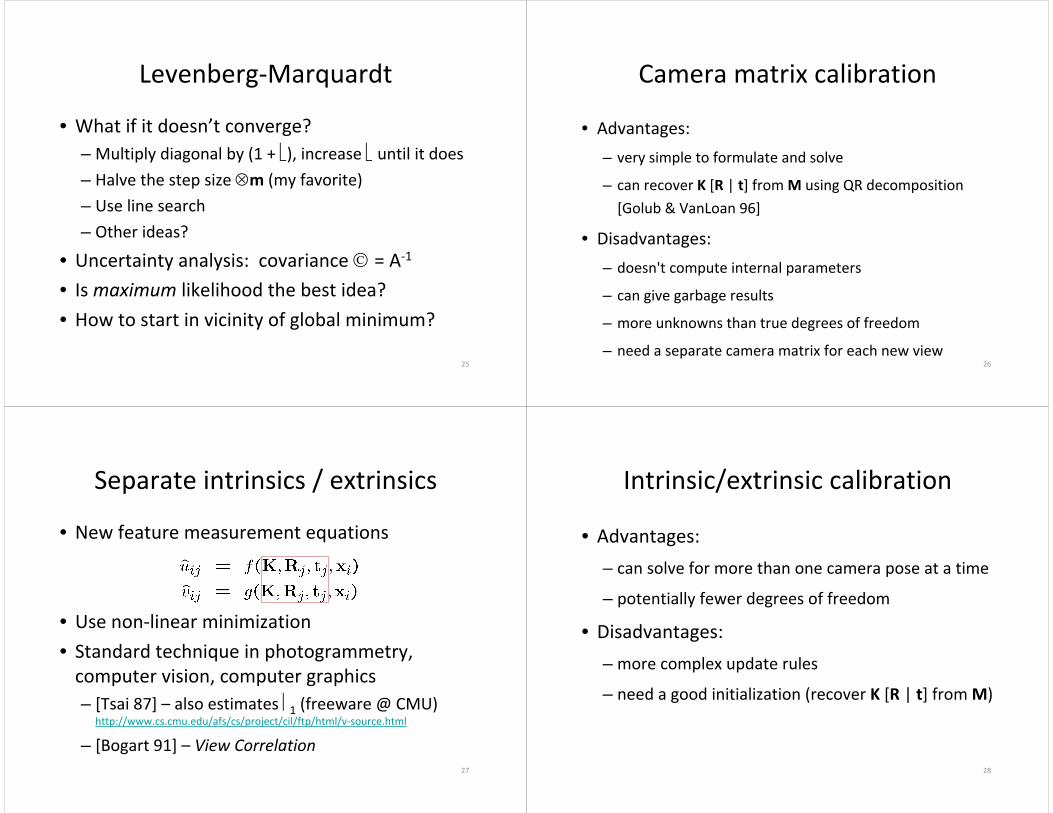
• What if it doesn’t converge?– Multiply diagonal by (1 + ⎣), increase ⎣ until it does– Halve the step size ⊗m (my favorite)

– Use line search

– Other ideas?

• Uncertainty analysis:  covariance © = A‐1

• Is maximum likelihood the best idea?

• How to start in vicinity of global minimum?

Levenberg‐Marquardt

26

Camera matrix calibration

• Advantages:

– very simple to formulate and solve

– can recover K [R | t] from M using QR decomposition 

[Golub & VanLoan 96]

• Disadvantages:

– doesn't compute internal parameters

– can give garbage results

– more unknowns than true degrees of freedom

– need a separate camera matrix for each new view

27

Separate intrinsics / extrinsics

• New feature measurement equations

• Use non‐linear minimization

• Standard technique in photogrammetry, computer vision, computer graphics– [Tsai 87] – also estimates ⎢1 (freeware @ CMU)

http://www.cs.cmu.edu/afs/cs/project/cil/ftp/html/v‐source.html

– [Bogart 91] – View Correlation28

Intrinsic/extrinsic calibration

• Advantages:

– can solve for more than one camera pose at a time

– potentially fewer degrees of freedom

• Disadvantages:

– more complex update rules

– need a good initialization (recover K [R | t] from M)

29

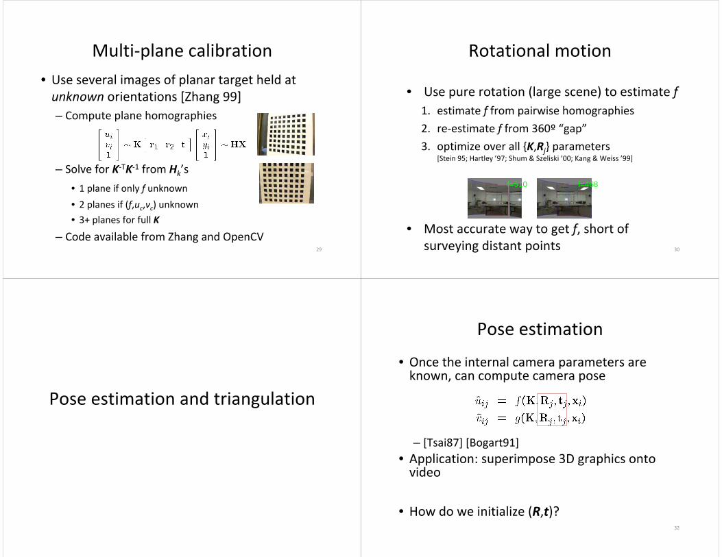
Multi‐plane calibration• Use several images of planar target held at unknown orientations [Zhang 99]– Compute plane homographies

– Solve for K‐TK‐1 from Hk’s

• 1 plane if only f unknown

• 2 planes if (f,uc,vc) unknown

• 3+ planes for full K

– Code available from Zhang and OpenCV30

Rotational motion

• Use pure rotation (large scene) to estimate f1. estimate f from pairwise homographies

2. re‐estimate f from 360º “gap”

3. optimize over all {K,Rj} parameters[Stein 95; Hartley ’97; Shum & Szeliski ’00; Kang & Weiss ’99]

• Most accurate way to get f, short of surveying distant points

f=510 f=468

Pose estimation and triangulation

32

Pose estimation

• Once the internal camera parameters are known, can compute camera pose

– [Tsai87] [Bogart91]• Application: superimpose 3D graphics onto video

• How do we initialize (R,t)?

33

Pose estimation

• Previous initialization techniques:– vanishing points [Caprile 90]

– planar pattern [Zhang 99]

• Other possibilities– Through‐the‐Lens Camera Control [Gleicher92]: differential update

– 3+ point “linear methods”:

– [DeMenthon 95][Quan 99][Ameller 00]

34

Pose estimation

• Use inter‐point distance constraints– [Quan 99][Ameller 00]

– Solve set of polynomial equations in xi2p

– Recover R,t using procrustes analysis.

u

(Xc,Yc,Zc)ucf

35

Triangulation

• Problem:  Given some points in correspondence across two or more images (taken from calibrated cameras), {(uj,vj)}, compute the 3D location X

36

Triangulation

• Method I: intersect viewing rays in 3D, minimize:

– X is the unknown 3D point– Cj is the optical center of camera j– Vj is the viewing ray for pixel (uj,vj)

– sj is unknown distance along Vj

• Advantage: geometrically intuitive

Cj

Vj

X

37

Triangulation

• Method II: solve linear equations in X– advantage: very simple

• Method III: non‐linear minimization

– advantage: most accurate (image plane error)

Structure from Motion

39

Structure from motion• Given many points in correspondence across several images, {(uij,vij)}, simultaneously compute the 3D location xi and camera (or motion) parameters (K, Rj, tj)

• Two main variants: calibrated, and uncalibrated (sometimes associated with Euclidean and projective reconstructions)

Orthographic SFM

[Tomasi & Kanade, IJCV 92]

41

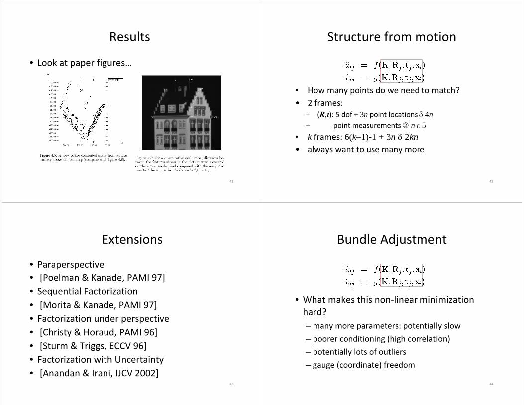
Results

• Look at paper figures…

42

Structure from motion

• How many points do we need to match?• 2 frames:

– (R,t): 5 dof + 3n point locations δ 4n– point measurements ® n ε 5

• k frames: 6(k–1)-1 + 3n δ 2kn• always want to use many more

43

Extensions

• Paraperspective• [Poelman & Kanade, PAMI 97]• Sequential Factorization• [Morita & Kanade, PAMI 97]• Factorization under perspective• [Christy & Horaud, PAMI 96]• [Sturm & Triggs, ECCV 96]• Factorization with Uncertainty• [Anandan & Irani, IJCV 2002]

44

Bundle Adjustment

• What makes this non‐linear minimization hard?– many more parameters: potentially slow

– poorer conditioning (high correlation)

– potentially lots of outliers

– gauge (coordinate) freedom

45

Lots of parameters: sparsity

• Only a few entries in Jacobian are non‐zero

46

Robust error models

• Outlier rejection– use robust penalty appliedto each set of jointmeasurements

– for extremely bad data, use random sampling [RANSAC, Fischler & Bolles, CACM’81]

Structure from motion

• Input: images with points in correspondence      pi,j  = (ui,j,vi,j)

• Output• structure: 3D location xi for each point pi• motion: camera parameters Rj , tj

• Objective function: minimize reprojection error

Reconstruction (side) (top)

SfM objective function• Given point x and rotation and translation R, t

• Minimize sum of squared reprojection errors:

predictedimage location

observedimage location

Scene reconstruction

Feature detection

Pairwisefeature matching

Incremental structure 

from motion

Correspondence estimation

Feature detectionDetect features using SIFT [Lowe, IJCV 2004]

Feature detectionDetect features using SIFT [Lowe, IJCV 2004]

Feature detection• Detect features using SIFT [Lowe, IJCV 2004]

Feature matching• Match features between each pair of images

Feature matchingRefine matching using RANSAC [Fischler & Bolles 1987] to estimate fundamental matrices between pairs

Reconstruction

1. Choose two/three views to seed the reconstruction.

2. Add 3d points via triangulation.

3. Add cameras using pose estimation.

4. Bundle adjustment

5. Goto step 2.

Two‐view structure from motion

• Simpler case: can consider motion independent of structure

• Let’s first consider the case where K is known– Each image point (ui,j, vi,j, 1) can be multiplied by K‐1 to form a 3D ray

– We call this the calibrated case

K

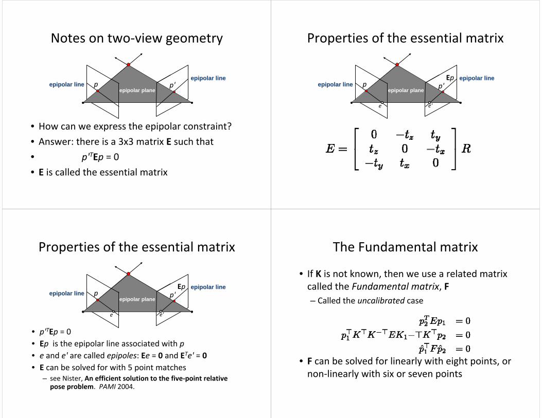
Notes on two‐view geometry

• How can we express the epipolar constraint?

• Answer: there is a 3x3 matrix E such that 

• p'TEp = 0

• E is called the essential matrix

epipolar plane

epipolar lineepipolar lineepipolar lineepipolar line p p'

Properties of the essential matrix

epipolar plane

epipolar lineepipolar lineepipolar lineepipolar line p p'

Ep

e e'

Properties of the essential matrix

• p'TEp = 0• Ep is the epipolar line associated with p• e and e' are called epipoles: Ee = 0 and ETe' = 0• E can be solved for with 5 point matches

– see Nister, An efficient solution to the five‐point relative pose problem.  PAMI 2004.

epipolar plane

epipolar lineepipolar lineepipolar lineepipolar line p p'

Ep

e e'

The Fundamental matrix

• If K is not known, then we use a related matrix called the Fundamental matrix, F– Called the uncalibrated case

• F can be solved for linearly with eight points, or non‐linearly with six or seven points

Photo Tourism overview

Scene reconstruction

Photo ExplorerInput photographs Relative camera positions 

and orientations

Point cloud

Sparse correspondence