overtaking assistance slutgiltig2x

Overtake assistance

Examensarbete utfört i fordonssystem av

Tomas Backlund

LiTH-ISY-EX--10/4328--SE

Linköping 2010

Overtake assistance

Examensarbete utfört i fordonssystem

LiTH

Handledare:

Examinator:

Linköping, 9 Mars, 2010

iii

Overtake assistance


av

Tomas Backlund

LiTH-ISY-EX--10/4328--SE

Erik Hellström

Linköpings Universitet

Henrik Pettersson

Scania CV AB

Jan Åslund

Linköpings Universitet

Mars, 2010

Overtake assistance


v

Biblioteksblad

vii

Abstract This thesis is about the development of a function that assists the driver of a

heavy vehicle to do an estimation over the possibilities to overtake a

preceding heavy vehicle. The function utilizes Look-Ahead and vehicle-to-

vehicle communication to do a calculation of the distance between the

vehicles in some road distance ahead. Consequently the report also contains

an investigation of what data that is needed to be known about a vehicle to

be able to do a satisfying estimation about this vehicle. The most vital

problem is to estimate what velocity the vehicle will get in an uphill/downhill

slope. A Simulink model is developed to simulate the function with two

independent vehicles. Real tests are also performed to evaluate the velocity

estimation part of the function.

ix

Acknowledgments

I would like to thank my supervisors Henrik Pettersson at Scania and Erik

Hellström at Linköpings Universitet for all their support and input to the

thesis. I would also like to thank all colleagues at REP for taking time to

answering my questions and giving inputs. A special thank to Rickard

Lyberger for his help with the GPS and road slope units to the test vehicles.

Tomas Backlund

Södertälje, 2010

xi

Content

Chapter 1 Introduction ..................................................................... 1

1.1 Background ....................................................................................... 1

1.2 Goals ................................................................................................. 1

1.3 Constraints ........................................................................................ 2

1.4 Outline .............................................................................................. 2

1.5 Related work ..................................................................................... 2

Chapter 2 Technology ...................................................................... 3

2.1 Look-Ahead ....................................................................................... 3

2.2 Communication ................................................................................. 3

2.3 CAN-Network .................................................................................... 4

2.4 Opticruise .......................................................................................... 4

Chapter 3 Problem description ......................................................... 5

3.1 Introduction ...................................................................................... 5

Chapter 4 Algorithm ......................................................................... 9

4.1 Uphill velocity ................................................................................... 9

4.2 Downhill velocity ............................................................................. 11

4.3 Basic vehicle dynamics .................................................................... 11

4.4 The distance calculation ................................................................. 15

4.5 Parameters ...................................................................................... 15

4.6 Data flow ......................................................................................... 17

4.7 Process flow .................................................................................... 18

Chapter 5 Simulations ..................................................................... 21

5.1 Introduction .................................................................................... 21

5.2 Level road simulations .................................................................... 22

5.3 Uphill simulations ........................................................................... 23

5.4 Downhill .......................................................................................... 28

5.5 Mass error test ................................................................................ 29

Chapter 6 Real test .......................................................................... 33

6.1 Test 1 Power mode ......................................................................... 33

6.2 Test 2 Normal mode ....................................................................... 36

Chapter 7 Conclusions ..................................................................... 39

Chapter 8 Future work .................................................................... 41

References ....................................................................................... 43

1

Chapter 1

Introduction

1.1 Background

It is a big difference between driving a heavy vehicle compared to a

passenger car mainly because of the weight to power ratio. A car have a

huge power overflow and can most of the time maintain desired speed

within reasonable limits, while for a heavy vehicle the case is the opposite

with very low power compared to weight. This will have big influence in

uphill slopes where heavy vehicles may experience power deficit and

therefore will not be able to maintain their desired speed. A hauling mission

is often time constrained in several ways, the driver has limitation in driving

time, the cargo should be in time etc. This forces the driver to keep the

average speed as high as possible without violating speed limits. In hills

different vehicles will be able to keep different speed which may trigger the

drivers of faster vehicles to overtake other slower equipages. Many times it

is hard for the driver to estimate if it is feasible to overtake, or even if there

is an advantage of the overtaking. The possibility of a down slope afterwards

will probably make the heavier vehicle to gain more speed and it would be

unnecessary to pass that vehicle in the uphill.

Today many companies are researching the use of maps with extended road

information which gives the knowledge of the road topography ahead.

Continental’s eHorizon [1] and DaimlerChryslers’s PCC [2] are examples of

research in the area. The main purpose of these works has been to minimize

the fuel consumption by optimizing the speed with the topography. Scania

has together with Linköping University developed a similar system called

Look-Ahead [3]. This thesis will explore the possibilities to utilize the Look-

Ahead data to create a function that can help the driver with the decision if it

is feasible to overtake or not.

1.2 Goals

The goal is to develop an algorithm that can support the driver in overtake

situations, this also includes to determine which information that is needed

to be sent between the vehicles and the requirements of this information to

get a satisfying estimation of the overtaking possibilities.

2

1.3 Constraints

In this thesis all surrounding traffic is neglected, it is assumed that there is a

highway with two lanes and that the vehicles are equipped with a

communication system for data exchanging.

A function like this is dependent on a human behavior. Consequently one can

never know what choices the driver will do when driving up or down a hill.

The gear changing and other things like increasing the speed before entering

the hill are very essential for the time it takes to force the hill. To eliminate

the human factor it is assumed that the vehicles are running with cruise

control and are equipped with the automatic gear changing system

Opticruise.

1.4 Outline

The algorithm will be developed in Matlab/Simulink together with a vehicle

model for simulating different scenarios and road profiles. The thesis will

also contain a brief look at the communication and some real tests

performed with modules running the 802.11p protocol.

A Simulink model that can simulate two different vehicles independent from

each other will be implemented. The model is based on the work of Niclas

Lerede [4] which contains one vehicle model with a Look-Ahead module. The

model will be used to simulate these vehicles behavior in different road

profiles with varying mass and engines. The overtake recommendation

module will be implemented in the same model. Real tests in an appropriate

hill are performed to verify the velocity prediction in the function.

1.5 Related work The overtaking assistance can be said to be included in the relative new

concept ADAS (Advanced Driver Assistance Systems). These systems are

defined to support the driver e.g. adaptive cruise control, lane departure

warning system and Scania driver support.

There is not much work to find in the topic overtaking assistance and for the

heavy segment is there nothing to find.

A researcher in Netherlands, Geertje Hegeman, [5] has developed a system

for cars that gives recommendations when it is safe to overtake and has

been tested in a simulator on a couple of drivers with good results. This

system requires car-to-car communication to get a picture of the

surrounding traffic which is under development but a commercial product is

probably decades away.

BMW has a concept that is a kind of overtaking assistance [5]. The system,

called Dynamic Pass Prediction, analyses the road map to find road sections

where it is not suitable to overtake. Note that there is no recommendation

for sections where it is safe to overtake.

3

Chapter 2

Technology

2.1 Look-Ahead

Look-Ahead is a system that delivers information about the road ahead. This

information contains mainly road topography in form of altitude and slope

but can also contain other usable information like curvature, speed limits,

road id, etc. This can be used to optimize the speed in the known road, like

setting the cruise control to prevent the speed to increase in the end of an

uphill if there is a downhill afterwards or let the engine run in fuel cut when

retarding to a lower speed limit. These actions are desirable since they can

save fuel.

The module contains a GPS receiver and a road map which includes the road

information. The information is used to build up a so called horizon with

small segments by a length of about 20 meters. Every segment contains a

slope and an altitude for the actual segment. The total size of the horizon

depends on the available memory. As the vehicle moves forward the module

will add new segments and throw away passed segments so that the horizon

always will have the same total length.

2.2 Communication

In the future we will most likely have communication to exchange data

between cars and the roadside infrastructure. There is an organization called

Car2Car Communication Consortium [6] whose mission is to set a European

standard for this type of communication. IEEE has devoted an extended

version of the standard WLAN protocol IEEE 802.11 to ITS (Intelligent

Transport Systems). This extension is called IEEE 802.11p and operates in the

frequency band 5.9 GHz which is dedicated for ITS. One big difference from

the ordinary WLAN is that this protocol doesn’t need a central unit to

communicate. It is a kind of ad hoc network which means that when one

node reaches another they will automatically establish a connection,

however this raises a traffic routing problem. If there is no central unit that

can control the traffic and decide who are allowed to send must this be

solved internally between the nodes.

MAC (Medium Access Control) is the name of the layer that controls the data

traffic. In 802.11p the MAC layer uses EDCA (Enhanced Distributed Channel

Access) which is based on ordinary CSMA (Carrier Sense Multiple Access)

with collision avoidance. This means that when a node wants to send, it will

first listen to the channel and if it is free the node will send its message. If a

collision occurs anyway it will be discovered by the two colliding nodes and

4

they will resend after a random backoff time. Consequently no upper bound

in the time to channel access is guaranteed which is vital in vehicle-to-vehicle

applications where real time access often is required. The protocol has a kind

of solution to this problem that is a QoS (Quality of Service) mechanism

which means that data is divided in different priorities where high priority

data gets shorter backoff time.

2.3 CAN-Network

CAN (Controller Area Network) is a standard protocol for vehicle computer

communication. It is message based and a central unit is not needed. Every

computer in the vehicle sends messages with unique id in a determined

frequency or on demand. A message can e.g. contain engine speed and be

sent every second.

This makes it rather simple to add a new function to the vehicle. The function

can read desired messages and send new ones on the bus. One problem is

that there exists no standard for what messages that must be sent over the

CAN-network. So to make a manufacture independent solution can be rather

difficult.

There is a standard called SAE J1939 [7] which includes a number of

messages that must be sent. This standard was developed in US for their

heavy truck industry and became rather common among other heavy truck

manufacturers over the world, but there are no regulatory directives to use

this standard. Every J1939 message contains 8 bytes of data and a standard

header. Scania uses J1939 and some other messages beyond the standard.

The overtake function will as far as possible use messages from the J1939

standard.

2.4 Opticruise

Opticruise is the name of Scania’s AMT (Automated Manual Transmission). It

is based on a regular manual gearbox with a control system added to control

the gear changing which is performed by some actuators. In latest version

the clutch is also automated. An advanced strategy makes sure that in most

cases the correct gear for the moment will be chosen. The driver can

influence the strategy by choosing between a normal and a power program.

The power program gears down early and tries to obtain desired speed. The

normal program is more economic and will therefore aim to keep the engine

speed low.

5

Chapter 3

Problem description

3.1 Introduction

In this report all examples and simulations are about two vehicles. The

vehicle that is behind and wants to overtake is denoted by vehicle 1 and the

preceding vehicle is denoted by vehicle 2. See figure 3.1.1.

There are three cases to study; uphill, downhill and level road. A brief

description of their respective problem is stated below.

In an uphill the velocity will decrease depending on weight, engine power,

resistance and slope angle. The gear changing strategy will affect the time it

takes to force the entire hill. The driver behavior will have a big influence,

keeping the engine speed high will keep the velocity high. While more

economic driving, which means keeping the engine in the economic area

1000 – 1300 rpm, will result in a longer time to force the hill. For vehicles

with opticruise the selected strategy mode will affect the time.

The velocity will increase in downhill slopes depending on weight, resistance

and slope angle. Note that the engine can be neglected in the case when the

hill is steep enough to make the vehicle roll without engine power. The

velocity may exceed the desired cruise control speed and even the electronic

speed limit at 89 km/h. This situation is again driver dependent since the

driver can choose to actively brake the vehicle to keep desired speed or use

the DHSC (DownHill Speed Control) which will automatically brake the

vehicle to DHSC set speed using the retarder and exhaust brake. This speed is

typical some km/h more than the cruise control speed. DHSC is only available

in vehicles equipped with retarder.

On level ground neither weight nor power is relevant assuming that the

vehicles have enough power to maintain desired speed on level road. The

distance between the vehicles at the end of the known road line can be

calculated assuming that both vehicles maintain their current speed.

The conclusion is that there are a couple of parameters that is vital for the

way the vehicle behaves in a slope. These parameters, from both vehicles,

are therefore important for the vehicle who wants to overtake.

6

Figure 3.1.1 Illustration of two vehicles approaching an uphill slope

A common situation that is the base for this work is described below, figure

3.1.1 illustrates the situation:

Imagine that there is a 1 lane road which will became 2 lanes before the hill.

The driver of vehicle 1 is approaching vehicle 2 and the uphill slope is ahead

of them. Vehicle 1’s driver has no idea of what’s going to happen when they

enter the hill since the driver doesn’t know the weight or engine size of

vehicle 2. The driver can decide to overtake vehicle 2 in the hill but may risk

that the vehicle will not be able to increase its speed enough to pass the

entire preceding vehicle before the hill ends and be stuck in a situation

where he must retard and fall in behind again. A situation like that is of

course dangerous and not desirable.

Figure 3.1.2 Illustration of two vehicles with communication, GPS and Look-Ahead

In figure 3.1.2 some equipment is added. Vehicle 1 is now able to see the

topography ahead with the Look-Ahead module and the GPS. The

communication makes data exchange possible and vehicle 1 can receive

information about vehicle 2. A function can use this information to do an

estimation of the distance at the end of the known road and inform the

driver of vehicle 1 that overtaking is inappropriate. In this way misjudged and

dangerous situations can be avoided.

A similar situation can appear in a downhill slope. Passing a heavier vehicle

before a downhill slope can be inappropriate since the heavier vehicle may

increase its speed more than the overtaking vehicle.

7

Figure 3.1.3 Illustration of two vehicles approaching a downhill slope

The equipment could also be utilized to help the driver in other situations

like in a level segment on a “2+1-road” where the driver can be informed if

the two lane segment is long enough for overtaking.

The main task will be to calculate the velocity or in fact the time it takes to

travel the available horizon distance. The velocity is dependent of the

balance of the forces that affects the vehicle. These forces are the air

resistance, the friction between the wheels and the road, the resistance that

the gradient causes in uphill slopes and the opposite for downhill slopes and

finally the generated force of the engine. This report will deal with two

different ways to calculate the engine generated force. The first way is to use

the maximum torque that the engines can deliver and the other way is the

maximum engine power used.

9

Chapter 4

Algorithm

4.1 Uphill velocity

When calculating the velocity in uphill slopes two different ways to calculate

the propulsive force are developed. The first version will use the engine’s

maximum torque and the other will use the maximum power.

4.1.1 Maximum engine torque

This method is a very straight-forward way to calculate the force that is

delivered to the vehicle driving wheels since the maximal engine torque is

known and the wheel torque is a multiplication of the total gear ratio in the

driveline. Another advantage is the fact that maximum torque is an essential

value and therefore is the probability high that this value is available in

different manufacturers CAN-network. A look at the engine torque curve will

show further advantages.

Figure 4.1.1 Torque curve of a 6 cylinder, 12 liter diesel engine

The torque curve is rather flat between 1000 and 1400 rpm and does not

differ much from maximum torque. This is also the area that the engine most

often operates in. This is convenient when calculating with maximum torque

due to the big chance that there is, in most cases, correct force at the

wheels. However in long steep uphill probably most vehicles will operate in

the high power output area (see figure 4.1.2).

10

But there are not only advantages. A problem with this method is that the

force at the driving wheels is dependent on the gear ratio. In a steep uphill

slope will many heavy vehicles probably be forced to change gear, which

changes the propulsive force at the driving wheels even though the engine

generated force is the same. Therefore a kind of gear changing strategy is

needed in the calculations. To make it simple the algorithm will change one

gear down when engine rpm is less than 1000 and gear up when engine

exceeds 1400 rpm. There is also added approximately one second of zero

torque during gear changing due to the real behavior, it takes some time to

change gear.

4.1.2 Maximum power

This version is quite similar to the maximum torque version. The difference is

the way of calculating the propulsive wheel force. The engine maximum

power is used instead of maximum torque. The advantage is that the power

is the same in the entire driveline except for a small friction loss. This means

that a gear changing strategy is not needed. Gear ratios, final gear ratios and

wheel radius can be neglected. The disadvantage is that maximum power

output from the engine is at high engine speed, 1500 – 1900 rpm, in

moderate uphill the propulsive force probably will be overestimated and as

well in steep uphill at the beginning of a hill before the first gear change

occur.

Figure 4.1.2 Power curve of a 6 cylinder, 12 liter diesel engine

11

4.2 Downhill velocity

Figure 4.2.1 Least gradient for coasting point with different vehicle mass

Figure 4.2.1 [8] shows the least angle needed to get vehicles at different

weights to continue with same or increased speed without using engine

power. This is called coasting and the definition is that the engine should run

in fuel cut mode (no fuel is injected) while the vehicle keeps desired velocity.

At the point where the vehicle will start coasting the engine force will be

disabled in the equation (4.11) and the velocity at the end of the segment

will be decided by the balance of the remaining forces. The top velocity is set

to 90 km/h in the simulations.

4.3 Basic vehicle dynamics

The calculations will be based on a vehicle model, however, the model is

simplified; the driveline (engine, clutch, gearbox, final drive, drive shafts)

rotation inertia is neglected because of its small influence in this usage since

the mass is dominant at high gears. The losses in the driveline are also

neglected. The model contains equations for rolling resistance (4.4), air

resistance (4.3) and slope resistance (4.5). Two ways to calculate the

propulsive force from the wheels generated by the engine will be

represented (4.1 and 4.2).

12

Figure 4.1 Vehicle model

The gravity force results in a normal force (Fn) which the rolling resistance is

dependent of and a slope force (Fslope) which in steep slopes has most

influence of the total resistance which means that the vehicle mass has a big

influence since ��

Following equation is for the version that uses maximum torque to calculate

the propulsive force.

Where �� is the maximum engine torque, �� is the actual gear ratio, ��

is the final gear ratio, �� is the driving wheel radius.

�� (4.1)

13

For the maximum power version is following equation used instead.

Pengmax is the maximum power output from the engine, � is the vehicle

velocity.

�� is the air resistance coefficient which can vary depending on cab size and

bodywork, � is the cross sectional area, �� is the air density.

�� is the roll resistance coefficient this will vary depending on tires, pressure,

etc. ��!"#$ gives the normal force (Fn in figure 4.1). This model is rather

simple but sufficient for this thesis and also convenient when calculating

with different vehicles since few parameters gives a more general solution.

α is the slope angle. The slope is often given in percent but there is no need

for conversion since there for small angles will be the same as in degrees.

Newton’s second law gives:

Equation (4.6) is time dependent and will be used in calculations that are

based on Look-Ahead data which is position based, therefore it is convenient

to transform the equation to be position dependent:

�� %�� (4.2)

�� 12 �� ( (4.3)

��)** � ��!"#$ (4.4)

�+*), � ��#�-$ (4.5)

��. � �� / �� / ��)**/�+*), (4.6)

�. � 1� 0�� / �� / ��)**/�+*),1 (4.7)

2�23 � 2�

2#2#23 � 2�

2# � (4.8)

14

(4.6) and (4.8) gives:

Further this equation will be discretized which makes it possible to solve

numerically. This is also an advantage when calculating with the Look-Ahead

data which is sampled.

�456 is the vehicle velocity when it enters the segment k and the result of

the calculation �4is the velocity in the end of the segment. ∆# is the segment

length.

For the maximum power version will equation 4.10 be:

2�2# � 1

�� 0�� / �� / ��)**/�+*),1 (4.9)

�4 � �456 8 2�2# 9�456, #456;∆# (4.10)

�4 � �456 8 1� <�� 456 / 1

2 �� 456 / �� !"#$�456

/ �� #�-$�456 > ∆#

(4.11)

�4 � �456 8 1� ?%��

�456( / 12 �� 456 / �� !"#$

�456/ �� #�-$

�456 @ ∆#

(4.12)

15

4.4 The distance calculation

The ambition is to develop an algorithm that delivers a calculated distance

between two vehicles in an arbitrary distance ahead. This arbitrary distance

is limited by the length of the look-ahead horizon, which in the simulation

model is two km.

The algorithm approximates the time t1 (derived from the mean velocity of

all segments) it takes for vehicle 1 to travel from the nearest forward to the

last segment in the horizon. The same calculation is done for vehicle 2 which

is some given distance ahead of vehicle 1. The calculation starts from vehicle

2s nearest segment to the last which results in a travel time t2. With these

“estimated” times is the distance between the vehicles at the end of the

horizon calculated, and in an arbitrary time will a new computation begins. In

this way is the algorithm delivering a new estimated vehicle distance a

horizon length ahead in real time.

The distance between the vehicles in the end of the horizon is calculated like

this:

The equation calculates the distance vehicle 2 have driven with its mean

velocity on the same time as vehicle 1 has been driven. Then the vehicle 1’s

distance is subtracted and the result is the distance between the vehicles if

they started at the same spot. Finally the actual distance is subtracted to get

the estimated distance ahead.

As desired are all three cases; level road, uphill and downhill, covered in the

same function.

4.5 Parameters

As shown in the equations, there are some important parameters that are

required from the preceding vehicle:

• Vehicle weight

• Engine maximum torque or power

• Vehicle GPS position

• Vehicle velocity

Vehicle weight is a very vital parameter. The weight is in Scania vehicles

estimated by different systems in the vehicle like brake system, opticruise

and engine control system. Currently the error margins are approximately

A#3��B3A2 �. 2�#3. � ?<#232 D 31 > / #1@ / B!3EBF �. 2�#3. (4.13)

16

±10%. Simulation with this error will be done to see the affect on the velocity

estimation.

Engine maximum torque can be found in the Scania CAN network as a

reference value for other engine torque variables which is given as a part of

this reference value.

Engine maximum power can be calculated from a J1939 message that

contains the engine torque at the engine speed where the engine delivers

maximum power.

Vehicle GPS position is currently not in the message standard but may follow

the Look-Ahead module in the future. Even though every vehicle won’t be

equipped with Look-Ahead, they will probably still have communication and

a GPS receiver.

Vehicle velocity is available in several CAN-messages in Scania. Vehicle speed

is a vital value for the tachograph which has regulated requirements in

correctness. The tachograph vehicle speed is sent on CAN.

Other data that is used:

In the algorithm is the actual distance between the vehicles used. This can be

calculated from the GPS-positions using the haversine formula [9].

Values that are used like roll resistance and air coefficient are not estimated

by the vehicle computers and can therefore not be sent. Maybe will this kind

of features exist in the future and the estimation will be more vehicle

specific. The friction coefficients in the model A, Cd and Cr are in this thesis

given typical values for heavy trucks.

G � 6371K� 9LB�3M �B2�E#; B � #�-( <∆FB3

2 > 8 !"#9FB36; D !"#9FB3(; D #�-( <∆F"-�2 >

2�#3 � G D 92 D B3B-29√B, √1 / B;

(4.14)

17

4.6 Data flow

Next page will show a data flow chart which is an overview of the containing

units and what data that is sent between them. This is the setup used in the

real tests later in the report.

Figure 4.6.1 shows the data flow between all including units. The CAN-bus is

of course central. The ICL block is the information cluster in the dashboard

which can show the information to the driver. Note that vehicle 2 doesn’t

need the Look-Ahead and map module as mentioned before.

Vehicle 1 GPS

Look-Ahead

+

Overtaking-

assistance

Road map

CAN

Velocity

Weight

Eng. info

Velocity v1, v2

Weight v1, v2

Pos. v1, v2

Eng. info v1, v2

Road data

Vehicle dist.

Recommend.

Com.

module

Velocity

Weight

Eng. info

Position

CAN Com.

module

Velocity

Weight

Eng. info

Position

GPS Position

Position

Road data

Vehicle 2 Velocity

Weight

Eng. info

ICL Vehicle dist.

Recommend.

Vehicle 2

Vehicle 1

Figure 4.6.1 Data flow for a vehicle set up with communication and Look-Ahead

18

4.7 Process flow

Next page shows a flowchart over the algorithm. The algorithm uses the

input velocity as initial velocity and calculates for a segment what the

velocity will be in the end of the segment. This will then be the input velocity

to the next segment. A mean velocity is calculated for the segment and from

that a travel time is derived. This time is accumulated in a total travel time.

This procedure is repeated until the entire horizon is processed. For vehicle 1

the calculation is performed from the first segment ahead of the vehicle.

When this is finished a travel time for the vehicle is obtained. To get a

correct estimation for vehicle 2 the calculation must start from the segment

that is just in front of vehicle 2. Therefore the numbers of segments from the

start of the horizon to vehicle 2 must be calculated. This is done by dividing

the distance between the vehicles with the segment length. The same

calculation as above is then performed for vehicle 2. The result is two total

travel times for the vehicles, together with their driven distance during this

time can the distance between them at the end of the horizon be calculated

with equation 4.13.

19

Last

segment in

horizon?

if vehicle # = 1 =>

Segment # = 1

if vehicle # = 2 =>

Segment # = Act. vehicle

dist/segment length

vin = Velocity vehicle #

Velocity vehicle 1, 2

Weight vehicle 1, 2

Engine power

vehicle 1, 2

Position vehicle 1, 2

Actual vehicle

distance

Look-Ahead horizon

Vehicle #

= 2?

Yes

Vehicle # =

2

If

Slope<coasting point

=> Engine power = 0

Calculate final velocity

vout for segment

Calculate travel time

for segment and add

to total time

No

Segment # + 1

vin = vout

Initialize

constants and variables

Vehicle # = 1

No

Calculate distance

between the

vehicles

Vehicle

distance

in

2000 m

Yes

Figure 4.7.1 Flow chart of the estimation calculation

21

Chapter 5

Simulations

5.1 Introduction

The simulations are done in Simulink and contain two vehicle models. The

vehicles can be configured individual in weight, engine model and cruise

control set speed. The initial distance between the vehicles can also be

selected. The vehicles will follow a road profile that is either generated from

a script or measured from a real road. The vehicles contain Look-Ahead

modules that work in the same way as the real module. A horizon is built

from the road profile in 20 meters segments with a total length of 2 km. The

overtake function module is modeled in vehicle 1 and gets its input directly

from the outputs in the model which means that the communication and

network dynamics is not simulated.

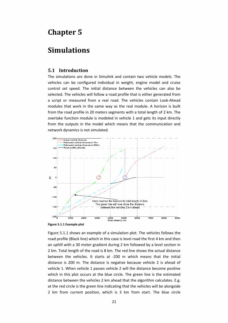
Figure 5.1.1 Example plot

Figure 5.1.1 shows an example of a simulation plot. The vehicles follows the

road profile (Black line) which in this case is level road the first 4 km and then

an uphill with a 30 meter gradient during 2 km followed by a level section in

2 km. Total length of the road is 8 km. The red line shows the actual distance

between the vehicles. It starts at -200 m which means that the initial

distance is 200 m. The distance is negative because vehicle 2 is ahead of

vehicle 1. When vehicle 1 passes vehicle 2 will the distance become positive

which in this plot occurs at the blue circle. The green line is the estimated

distance between the vehicles 2 km ahead that the algorithm calculates. E.g.

at the red circle is the green line indicating that the vehicles will be alongside

2 km from current position, which is 3 km from start. The blue circle

22

indicates the red line that the vehicles are aside at position 5 km from start.

The blue line shows the estimated distance in 600 m, this is plotted to see if

the estimation is more accurate closer to the vehicle.

Two more notable effects of the algorithm can be seen.

Firstly, between 0 – 1200 m it looks like the estimated distance between the

two vehicles rapidly increases, however this is not the case, it is caused by

the building of the horizon. In the beginning of the simulation the total

horizon is not known for the estimation and it takes a number of samples to

build the full horizon. Hence, the estimation before 1200 m is not calculated

for 2 km but for a shorter and increasing distance.

Secondly, when vehicle 1 overtakes vehicle 2 the estimation stops. This is

due to the implantation of the algorithm, it can’t do an estimation for a

vehicle that is behind. The reason for this is because it is assumed that when

the two vehicles are aside the overtake has begun and therefore is

irreversible.

5.2 Level road simulations

Simulation setup:

Vehicle 1 Vehicle 2

Weight: 60000 kg 30000 kg Engine: S6 S6 Displacement: 12 liter 12 liter Max power: 480 hp 420 hp Max torque: 2350 Nm 2100 Nm CC speed: 82 km/h 80 km/h

Figure 5.2.1 Estimated distance on level road with constant speed

Figure 5.2.1 shows the behavior on level road, the estimation is correct

which confirms that the distance calculation works as desired. This is of

23

course only if no change in speed is done. Next simulation will show what

happens if vehicle 1 accelerates from 80 km/h to 85 km/h. Same setup as

preceding simulation.

Figure 5.2.2 Estimated distance on level road with speed change

Figure 5.2.2 shows that both vehicles are traveling in 80 km/h, vehicle 2

begins 200 meter ahead of vehicle 1. At 2800 meter from start vehicle 1’s

speed increases to 85 km/h and the distance between the vehicles will start

to decrease. As shown in the figure the estimation is changing instantly. This

is a grateful feature since the driver instantly will be informed about the new

distance during changes in speed.

5.3 Uphill simulations

These simulations will contain a comparison between the power and the

torque version. It is only in uphill slopes that this will have an effect on the

vehicle velocity.

5.3.1 Power version simulation 1

The simulated situation is that vehicle 1 is approaching vehicle 2 and a hill is

upcoming. It is now of interest to see if the estimation could help the driver

of vehicle 1 to decide if overtaking is possible. The estimating function uses

the power version in the calculations.

Simulation setup:

Vehicle 1 Vehicle 2


24

Figure 5.3.1 Estimated distance in uphill slope, different vehicles with constant speed

Figure 5.3.1 shows the situation where the driver of the vehicle behind

already before the hill can see that his vehicle has passed the preceding

vehicle with 100 m in about 2 km (notice the green line at 4000 m). From

that information a decision about overtake can be taken which in this case is

to prefer since vehicle 1 won’t lose any speed while vehicle 2 lose about 5

km/h (see figure 5.3.2).

Figure 5.3.2 Speed calculation vs. simulated speed

Figure 5.3.2 shows the velocity that the algorithm is estimating in its

calculation which is the basis for the distance estimation. The velocity is

compared with the simulated velocity which decides the “real” distance. The

graph shows a miscalculation with about 1 km/h this is reflected in the

distance estimation as the estimated distance differs a bit from the

simulated. The notch in the black line at approximately 5700 meters is due to

25

a gear shift, the black line shows an overshoot at 6000 meter which depends

on the cruise control regulator in the model.

5.3.2 Power version simulation 2

This simulation will have the same setup as previous but with switched

weights, vehicle 1 is now the heavier one.

Figure 5.3.3 Estimated distance in uphill slope, different vehicles with constant speed

Imagine that the situation for the driver is the same as the preceding

simulation. Before the hill the driver will instead be informed that the

distance will increase in the hill and overtaking will be impossible (compare

figure 5.3.1 to figure 5.3.3).


26

The figure shows almost perfect velocity estimation. The small error is

reflected in the distance estimation as the strange bends in the green line at

5000 m (figure 5.3.3).

5.3.3 Torque version simulation 1

Following simulations will be the same as above but this time will the torque

version be used in the calculations.

Figure 5.3.5 Estimated distance in uphill slope


27

These figures correspond to the figures 5.3.1 and 5.3.2. They are quite

similar to the power version, which means that the both versions show

similar functionality, however the power version is simpler.

5.3.4 Torque version simulation 2

Same simulation as for the power version with switched weights, vehicle 1 is

the heavier one.

Figure 5.3.7 Estimated distance in uphill slope


28

Figure 5.3.8 shows that the torque version miscalculates the velocity for

vehicle 1. This error is reflected in the distance estimation (figure 5.3.7) at

approximately 4500 meter. The strange behavior at that point depends on

the miscalculation in the velocity. When the vehicle reaches the earlier

estimated section the error is induced in the distance estimation since the

distance became another than expected. This shows the problem with the

torque version when there is a big decrease in speed and gear changing is

needed. Note that the power version handles this situation in a better way.

5.4 Downhill

5.4.5 Simulation 1

This simulation will show the behavior in a downhill slope.

Simulation setup:

Vehicle 1 Vehicle 2


Figure 5.4.1 Estimated distance in downhill slope

This figure shows that the function did not calculate entirely correct. The

reason will be shown in the next figure.

29


The calculated velocities don’t match with the simulated model. The reason

for this is probably that the simulation model is more advanced than the

calculation in the algorithm. That there are errors in the model cannot be

excluded. Real tests later in the report shows more satisfying match.

5.5 Mass error test

The vehicle weight has a big influence of the calculation. As mentioned

before the error margin are ±10 % which means that the deviation can be up

to 6 tons for a 60 tons equipage. Therefore a test is interesting to see the

effect on the velocity estimation.

A simulation is performed with the power version, vehicle 2’s mass input to

the function is modified ±10 %

Simulation setup:

Vehicle 1 Vehicle 2


30

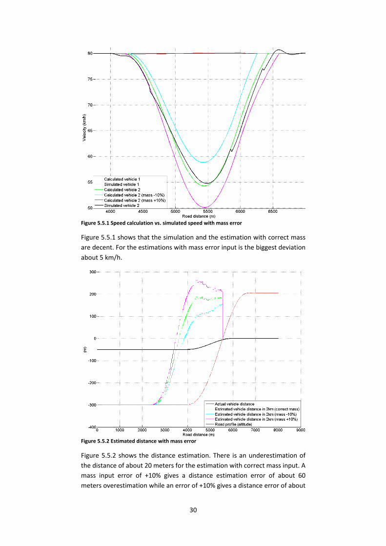
Figure 5.5.1 Speed calculation vs. simulated speed with mass error

Figure 5.5.1 shows that the simulation and the estimation with correct mass

are decent. For the estimations with mass error input is the biggest deviation

about 5 km/h.

Figure 5.5.2 Estimated distance with mass error

Figure 5.5.2 shows the distance estimation. There is an underestimation of

the distance of about 20 meters for the estimation with correct mass input. A

mass input error of +10% gives a distance estimation error of about 60

meters overestimation while an error of +10% gives a distance error of about

31

100 meters underestimation. This is read at the road position 4500 meters

where the estimation reaches the final value for the distance. As seen in the

figure the estimation is continuing towards a more correct value. This fault

will be doubled if the first vehicle is +10% wrong and the other -10% wrong.

This means that a fault margin of at least 120 meters is needed in this case.

33

Chapter 6

Real test

This test is performed to observe the real behavior and compare with the

velocity estimating function of the algorithm. The test is performed with two

different vehicles in the hills between Åby and Stavsjö outside of Norrköping.

Vehicle 1: Scania R620 Tractor with semi-trailer Gearbox: Opticruise Weight: 39000 kg (measured) Engine: V8 Displacement: 16 liter Max power: 620 hp Max torque: ~ 3000 Nm

Vehicle 2: Scania R420 Rigid truck with full-trailer Gearbox: Manual Range/Split Weight: 37000 kg (measured) Engine: S6 Displacement: 12 liter Max power: 420 hp Max torque: ~ 2100 Nm

The vehicles were equipped with GPS receivers and communication modules

with the 802.11p protocol. Vehicle 1 was furthermore equipped with an

extension module that calculated the actual slope angle. The slope is used to

evaluate the velocity estimating part of the function. It would of course be

desirable to have the entire overtake function available in the vehicle

computer for instant testing but there is a lot of adoption needed to make

that possible. Vehicle 2 sends its GPS-position and velocity to vehicle 1.

Everything was recorded with CANalyzer which is a program that makes it

possible to record the activity on the CAN-bus. These log files are then used

to evaluate the function through a couple of scripts which results are shown

in plots.

6.1 Test 1 Power mode

Vehicle 1 and 2 are driving with cruise control in 89 km/h, vehicle 2 begins

approximately 65 meter ahead of vehicle 1. Vehicle 1 has the opticruise in

power mode, vehicle 2 is driving like a regular driver would do with a manual

gearbox, however it is rather difficult to know how a driver “normally” will

act, but most probably keeping velocity as high as possibly is a good premise.

Vehicle 2 is therefore geared down early to 11th gear which proved to be

34

enough and is held trough the entire hill. This will hopefully show a good

match with the calculation because of the early maximum power output.

Figure 6.1.1 Real test Åby – Stavjö OPC in power mode

Figure 6.3.1 shows the measured velocity and the velocity that the algorithm

calculates with equation 4.11.

Unfortunately the slope measurement is of quite low quality since the test

vehicle was missing the correct equipment to get an accurate movement

input. This is needed since the slope angle is calculated from the altitude

change in a given movement. This will affect the calculated velocity since

equation 4.11 is based on the slope angle.


Figure 6.1.2 is an enlargement of the first hill area in figure 6.1.1 which

shows that the velocity calculation is decent but the less satisfactory slope

data affect the calculation (see figure 6.1.2 at ~4000m).

35

The curves of vehicle 2 matches good which, as expected, is a result of the

high power output when entering the hill. The power output of vehicle 1 is

delayed because the opticruise didn’t gear down before entering the hill.

This is because the control system must discover a power deficit and must

consequently sense the slope before a gear changing is decided.


Figure 6.1.3 shows an enlargement of the last downhill in figure 6.1.1. The

coasting calculation seems to work fine, Vehicle 1 and 2 have almost the

same weight and would therefore coast quite similar which is the case for

the calculation. Vehicle 1 differs from the calculation and from vehicle 2

which depends on the driver who is using the DHSC (Down Hill Speed

Control) with set speed at approximately 92 km/h.


Figure 6.1.4 shows the distance between the vehicles during the same

measurement as above. This distance is calculated from the vehicle’s GPS

positions according to equation 4.13. Vehicle 1 is passing vehicle 2 at 150

36

seconds from start. The interferences occur when the connection is lost,

which seems to be a quite periodic and may be depending on the test

versions of the communication equipment. In any case the interferences can

to a certain extent be compensated by dead reckoning the positions during

connection loss.

6.2 Test 2 Normal mode

Figure 6.2.1 Real test Åby – Stavjö OPC in normal mode

Figure 6.2.1 shows the same road section as figure 6.1.1 but this time is

vehicle 1 running with opticruise in normal mode. Vehicle 2 is running in the

same way as before with high power output.

37


Figure 6.2.2 shows an enlargement of the same section as figure 6.1.2. Here

it is quite clear that the normal mode differs a lot from the power mode

consequently will the velocity differs much from the calculated. The

estimation for vehicle 2 is again satisfying.


Figure 6.2.3 shows the same road section as figure 6.1.3. This is the downhill

slope and the power mode selected doesn’t matter here. Unlike the previous

downhill measurement both vehicles are now running without DHSC and as

38

expected before, both vehicles are now coasting similar. The estimation

shows decent results.


Figure 6.2.4 shows the distance between the vehicles during the

measurement. The maximum distance is this time approximately 300 m

compared to 400 m in figure 6.1.4. This means that the difference in this

road section between power and normal mode is approximately 100 meters.

The consequence of the difference the driver selected gear mode generates

can be illustrated by following example.

Imagine that the initial distance was 365 meters instead of 65. This would in

the first case with power mode result in a maximal vehicle distance of 100

meters and an overtake would be succeeded. The same situation in case 2

with normal mode would end up in a failure since the vehicles would have

ended up aside and the overtake would fail.

39

Chapter 7

Conclusions

The challenge is as with many other functions to develop a vehicle model

that corresponds satisfyingly to the reality and even more challenging if a

human behavior is a factor of influence. In the simulations the human factor

is neglected and the vehicles are strictly following their cruise controllers. A

real behavior is more dynamic, the driver can slow down when approaching

a vehicle and speed up when passing etc. The simulations show that a

relatively good performance is obtained when the “simulated” reality

conforms to the estimation, of course is there a bad result when there is a

big deviation in the velocity estimation. An interesting behavior is that this

deviation often occurs in the beginning of a hill. This is because of the

calculation with maximum power output. The simulation model’s gear

changing logic is very simplified compared to the Opticruise which explains

the bad matching in the beginning of the uphill slopes. The real test confirms

that it matches better if high power output is performed early when entering

the hill (figure 6.1.2). More tests are needed to evaluate the estimation in

other situations. If the matching is that good when using high power output

the possibilities that the function can be useful is increased. Imagine an

overtake situation, the vehicle that wants to overtake will probably gear

down early and use the engine maximally. The function will then estimate

the own vehicle correct and overestimate the preceding vehicle. If the

preceding vehicle also uses the engine maximally the estimation will be

correct for both vehicles. This means that the recommendation is either

underestimated or correct which will end up in a successful overtake. The

situation where a recommendation will fail is if the driver who wants to

overtake doesn’t use the engine maximally and the preceding vehicle does.

The conclusion is that if the overtake will succeed or not is in the end up to

the driver that uses the function. This is of course if assumed that all input

data is correct.

The fact that there can be errors in the input data to the function still exists.

It is showed in chapter 5.5 that a mass error will affect the estimated

velocity. Real tests with the function will show the affect of the distance

calculation and from that can the mass accuracy requirements be stated.

Another error source is the road map data, the slope must be significantly

better than our measurements. This is probably not impossible since there

are very accurate tools for this kind of measuring. Another error source is the

GPS-positioning, the absolute position accuracy is about 20 meters

depending on number of satellites connected, but the relative distance

between 2 nodes that are close to each other should be rather good since

40

they probably will be connected to the same satellites. More real tests must

be performed to evaluate this and for the influence of other variables like

roll and air resistance coefficient.

Of the two ways of calculating the propulsive force is the maximum power

version most advantageous because of the simple calculation and few

dependencies of vehicle specific properties. Their results are rather similar in

the simulated tests which can depend on the fact that gear ratios, final gear

ratio and wheel radius is the same both in the model and in the calculations.

Real tests with different vehicle specifications will probably show worse

results from the torque version and even more worse in steep hills with

many gear changes.

The requirements of the communication are relatively small compared to the

capacity of the equipment that was used in the measurements. The

information between the vehicles was sent with 100 times higher frequency

than needed and there were no capacity problems.

41

Chapter 8

Future work

The Simulink implemented function must be adapted to the real Look-Ahead

module and to read data from CAN instead of the Simulink vehicle model. As

mentioned before more tests and validation are needed with the entire

function in the test vehicle. When that work is done a discussion about the

margins for a recommendation remains. Depending on the reliability of the

function, a minimum vehicle distance can be set for the recommendation.

Let’s say that the overtaking vehicle must have passed with at least 100 m in

the estimation before a recommendation. Assumed that the function doesn’t

overestimate this value, maybe accuracy at ± 20 meters can be allowed for a

100 meters margin. A first step can be to adopt the way BMW is thinking

with its Dynamic Pass Prediction, just tell the driver when an overtake is

impossible.

43

References

1. Dr. R. Varnhagen, Continental Automotive GmbH. Reduction of fuel

consumption with intelligent use of navigation data, Wetzlar.

2. F. Latteman, K. Neiss, S. Terwen, T. Connolly. The predictive cruise control

- A system to reduce fuel consumption of heavy duty trucks, SAE Technical

paper, 2004.

3. Hellström, Erik. Look-ahead control of heavy truck utilizing road

topography, Licentiate thesis, Linköpings universitet, 2007.

4. Lerede, Niclas. Topography based fan control for heavy trucks, Master

thesis, Linköpings universitet, 2009.

5. Overtaking assistant could help prevent many traffic-raelated deaths,

Science Daily [Online] 26/01/2010

www.sciencedaily.com/releases/2008/02/080226092749.htm

6. Car2Car Communication Consortium [Online] 26/01/2010

www.car-to-car.org

7. Wikipedia [Online] 26/01/2010, http://en.wikipedia.org/wiki/J1939.

8. Fröberg, Anders. Simulation and Optimal Control for Vehicle Propulsion,

PhD thesis, Linköpings universitet, 2008.

9. Movable Type Scripts [Online] 26/01/2010

http://www.movable-type.co.uk/scripts/latlong.html

Al Alam, Assad. Optimal fuel efficient speed adaption, Master thesis, Royal

Institute of Technology, 2007.

Lars Eriksson and Lars Nielsen, Modeling and control of engines and

drivelines, Vehicular Systems, Linköping 2008

overtaking assistance slutgiltig2x

Documents