overstrand to walcott strategy study - north norfolk · overstrand to walcott strategy study ......

Overstrand to WalcottStrategy Study

CliffSCAPE modelling and clifftoprecession analysis

Part II: Technical Support Information

Report EX 4692June 2003

Overstrand to Walcott Strategy Study

CliffSCAPE modelling and clifftop recession analysis



��Address and Registered Office: HR Wallingford Ltd. Howbery Park, Wallingford, OXON OX10 8BATel: +44 (0) 1491 835381 Fax: +44 (0) 1491 832233

Registered in England No. 2562099. HR Wallingford is a wholly owned subsidiary of HR Wallingford Group Ltd.

�� ii EX4692 Part II – Technical Support Information 16/07/03

�� iii EX4692 Part II – Technical Support Information 16/07/03

Contract - Consultancy

This report describes work commissioned by North Norfolk District Councilwhose representative was Mr Peter Frew. The HR Wallingford job numbers wereCDR3212 and CDR3214. The work was carried out by Dr Jim Hall and Dr MikeWalkden of the University of Bristol. The HR Wallingford project manager wasMr Paul Sayers.

Prepared by ...........................................................................................

(name)

...........................................................................................

(Title)

Approved by ...........................................................................................

(name)

...........................................................................................

(Title)

Authorised by ...........................................................................................

(name)

...........................................................................................

(Title)

Date............................................

© HR Wallingford Limited 2003

HR Wallingford accepts no liability for the use by third parties of results or methods presented in this report.

The Company also stresses that various sections of this report rely on data supplied by or drawn from third partysources. HR Wallingford accepts no liability for loss or damage suffered by the client or third parties as a resultof errors or inaccuracies in such third party data.

�� iv EX4692 Part II – Technical Support Information 16/07/03

�� v EX4692 Part II – Technical Support Information 16/07/03

Summary

Overstrand to Walcott Strategy Study

CliffSCAPE modelling and clifftop recession analysis



A numerical model study of a section of the North Norfolk coast has beenconducted to predict the effect of alternative strategic coastal management options,including ‘do nothing’, ‘do minimum’ and higher cost schemes. The studycombined a regional-scale version of the cliffSCAPE soft cliff and platformerosion model with a stochastic model of coastal landsliding.

CliffSCAPE provides a prediction of the response of the shoreline (cliff toe) tochanges in coastal management and other long term coastal changes (for exampleclimate change). The stochastic model uses predictions from cliffSCAPE togetherwith information from cliff surveys to generate a probabilistic prediction of clifflocation that can be used in the economic appraisal of strategic coastalmanagement options.

This study was the first application of cliffSCAPE as a regional modelling tool forsoft cliff shorelines. The results of the validation process are very positive,indicating a good match between model output and historic records of shorerecession over three eras spanning a total of 87 years. However, cliffSCAPE haspreviously been applied at only one other coastal site (the Naze on the Essexcoast) and has never been applied to such a long length of coastline as examined inthis study. Thus, the results may be considered experimental, as cliffSCAPE stillrequires testing and validation on a wider range of coastal sites.

The cliff evolution modelling has been used to predict future changes in clifftopposition under a range of management scenarios. The models indicate that thecliff system is strongly influenced by sediment transport rate, with recession ratesin particular areas strongly dependent on both current and historic managementdecisions both locally and up-drift.

�� vi EX4692 Part II – Technical Support Information 16/07/03

�� vii EX4692 Part II – Technical Support Information 16/07/03

ContentsTitle page iContract iiiSummary vContents vii

1. Introduction ................................................................................................ 1

2. The cliffSCAPE model............................................................................... 1

3. Setup of the cliffSCAPE model for the North Norfolk coast ..................... 2

4. Model validation......................................................................................... 44.1.1 Profile development ......................................................... 44.1.2 Plan shape development ................................................... 5

4.2 5 Scenario testing .......................................................................... 74.2.1 Scenario 1, ‘Open coast’ .................................................. 74.2.2 Scenario 2, ‘Do Nothing’ ................................................. 84.2.3 Scenario 3, ‘SMP policy options’..................................... 94.2.4 Scenario 4, ‘Revised SMP policy options’..................... 114.2.5 Scenarios 5a – 5e, ‘SMP policy options with Groyne

Modification’.................................................................. 124.3 6 Sensitivity tests......................................................................... 14

4.3.1 Sensitivity to rate of sea-level rise.................................. 144.3.2 Sensitivity to residual life............................................... 16

5. A stochastic model of coastal cliff landsliding......................................... 17

6. Conclusions .............................................................................................. 21

7. References ................................................................................................ 22

TablesTable 1 Input parameters for cliffSCAPE RS................................................... 3Table 2 Summary of scenarios.......................................................................... 7Table 3 Summary of sensitivity tests .............................................................. 14Table 4 Cliff top recession prediction input data ............................................ 19

FiguresFigure 1 Flow chart representation of cliffSCAPE ............................................ 2Figure 2 The study site plan shape and cliffSCAPE cross-section positions ..... 4Figure 3 Model profile evolution at Mundesley, 25 year stages from 1600 to

2000 ..................................................................................................... 5Figure 4 Comparison between model recession rates and measurements

provided by Cambers ........................................................................... 6Figure 5 Recession resulting from an ‘Open coast’ management policy

(scenario 1)........................................................................................... 8Figure 6 Recession resulting from a 'Do Nothing' management policy

(scenario 2)........................................................................................... 9

�� viii EX4692 Part II – Technical Support Information 16/07/03

Contents continued

Figure 7 Recession resulting from a ‘SMP policy options’ managementpolicy (scenario 3) ..............................................................................10

Figure 8 Beach volume at section 58 under scenarios 2 and 3 .........................11Figure 9 Recession resulting from a revised ‘SMP policy options’

management policy (scenario 4) .........................................................12Figure 10 Results of scenarios 3 and 5a to 5d, 'SMP policy options with

groyne modifications', ‘GI’ indicates a location of groyneimprovement. ......................................................................................13

Figure 11 Average recession rates resulting from different rates of sea-levelrise (SLR), (scenarios 2, 3, 6a, 6b, 6c, & 6c)......................................15

Figure 12 Average recession rates resulting from three ‘Do nothing’management options, with different estimates of residual life (RL)(scenarios 2, 7a & 7c). ........................................................................16

Figure 13 Diagrammatic representation of the coastal landsliding model ..........17Figure 14 Layout of CBUs (coloured sections of coastline and small black

numbers) with cliffSCAPE sections overlaid (red lines and largenumbers) .............................................................................................18

Figure 15 Typical cliff top recession predictions (cliffSCAPE section 13 inScenario 1) ..........................................................................................20

AppendixOverstrand to Mundesley Strategy Study: cliff toe recession results

�� 1 EX4692 Part II – Technical Support Information 16/07/03

1. INTRODUCTION

This report describes a model study of the North Norfolk coast between Overstand and Mundesley. Theobjective of the study was to predict the effect of alternative strategic coastal management optionsincluding ‘do nothing’, ‘do minimum’ and higher cost schemes. The model study combined two modellingapproaches:

� a regional-scale version of the cliffSCAPE soft cliff and platform erosion model� a simple stochastic model of coastal landsliding.

CliffSCAPE provides a prediction of the response of the shoreline (cliff toe) to changes in coastalmanagement and other long term coastal changes (for example climate change). The stochastic model usespredictions from cliffSCAPE together with information from cliff surveys to generate a probabilisticprediction of cliff location that can be used in the economic appraisal of strategic coastal managementoptions.

2. THE CLIFFSCAPE MODEL

CliffSCAPE is a model of the process of shore platform lowering and cliff toe recession that governs theretreat of soft coastlines and their response to coastal management interventions. As well as representingthe in-situ shore platform and cliff toe, cliffSCAPE models the mobile beach, its role in protecting orabrading the platform and the contribution that cliff and platform sediments make to the mobile beach. Aregional-scale version of cliffSCAPE (cliffSCAPE-RS) is available to model long sections of coast forstrategic assessment purposes, whilst the local-scale version can better resolve the effects of individualbeach control and coast protection structures. Because of the strategic nature of the current study,cliffSCAPE-RS was chosen for the analysis.

A flow chart of cliffSCAPE-RS modelling tool is shown in Figure 1. CliffSCAPE-RS describes a two-dimensional shore section, which is made quasi-3D by using a series of such sections and allowinginteraction between them. The model time-step is 12.47 hours, i.e. one tidal period. Every time-step waveand tide data are sampled from synthetic time-series, which in this study were generated by HRWallingford. The synthetic wave data was generated for one offshore point, grid reference 636836,350606, which is approximately 18 km due north of Walcott. The waves are refracted using Snell’s Lawand shoaled over a topography that represent, in a simplified way, site bathymetry. A cross-shoredistribution of longshore sediment transport is calculated using tidal changes in water level and adistribution under static conditions published by McDougal and Hudspeth (1984). A similar approachprovides a cross-shore erosion distribution function. Potential sediment transport at each shore section iscalculated using the CERC equation (Shore Protection Manual 1984). The cross-shore distribution of driftis compared to the beach width to discern what proportion of the potential transport actually occurs. Themagnitude of erosion at different elevations across the shore is calculated using the duration of submersionduring the tidal cycle, location within the surf zone and local slope. These are combined with theexpression provided by Kamphuis (1987) for shore recession rate due to wave attack, and a distribution oferosion due to random waves under static water-level conditions obtained from Skafel & Bishop (1994)and Skafel (1995). Kamphuis’ expression provides the magnitude of recession; the results of Skafel areused to distribute it over the platform. Kamphuis’ expression was chosen because it provides an expressionin which wave breaking processes are well represented at the level of abstraction appropriate for themodel. Material strength is represented by a variable R, which is found during calibration by comparingaverage historical recession rates to measured values. Although Kamphuis justifies his expression he doesnot provide values for R or link it to measurable geotechnical parameters. The beach is considered toprotect the profile when it is of adequate thickness. Following field measurements of Ferreira (2000) thiswas defined as a depth of sand exceeding one-fifth of the wave height. If a thinner beach is present then itsprotective capability is assumed to vary linearly with depth of sand.. Once the whole profile has been


recalculated overhanging material above the cliff toe is assumed to collapse to form talus; a constant cliffangle was assumed for the calculation of talus volume. Talus was assumed to have one-tenth of thestrength of intact material. Not all of the material eroded from the talus was assumed to contribute to thebeach volume. The fraction of beach material was determined by the British Geological Survey.

Figure 1 Flow chart representation of cliffSCAPE

CliffSCAPE provides predictions of shore profile and cliff plan-shape evolution. The latter is of mostinterest for strategic-scale studies.

The relationship between measurable properties of a shore platform and its resistance to erosion by the seais unknown (Walkden et al, 2002). Any shore platform erosion model therefore has to be calibrated againsthistoric recession rates. CliffSCAPE is attractive in that, whilst it has to be calibrated in order to reproducepast average recession rates, differences in recession up and down the coast or across the shore platformare predicted by the model and can be compared with measurements. In this study, comparison betweendifferentials in average recession rates along the north Norfolk coast were used as the main criterion formodel evaluation; model output was compared to long-term recession rates published by Cambers (1976).

3. SETUP OF THE CLIFFSCAPE MODEL FOR THE NORTH NORFOLK COAST

CliffSCAPE is based on concepts of system equilibrium. Before a cliffSCAPE model can be expected tobehave in a realistic manner it must be allowed to develop towards a ‘balanced’. This applies to bothalongshore and cross-shore form; sediment released from the cliff must match sediment moved away bylongshore transport and the interaction between cross-shore shape and erosion (and inundation due torising sea-levels) result in an unchanging profile. As with the real coast, if the form is out of balance thensubsequent erosion will be too high or too low. The first step in this process is to produce a single cliffprofile using local wave, tide and sea-level rise conditions. The initial profile is assumed to be a verticalcliff plunging into deep water, i.e. intentionally far from equilibrium, and the model is run to simulateresponse to many hundred of years of wave and tide action. Once this cliff profile has stabilised it isreproduced to generate multiple sections, in this case there were 63. These were arranged side-by-sidealong a baseline to form a quasi three-dimensional coast with a model distance between them of 500metres. The baseline projected at an angle of 300 degrees (west-north-west) from grid reference640835,327250, which was its intersection with the first and most southerly profile. Appropriate offsetswere introduced to represent the coast plan shape, as illustrated in Figure 2 and a beach was introduced


(the exchange of beach material is calculated mid-way between sections). The model was then set to runagain to allow the profiles to respond to the presence of the beach, and also for balance to be reached in thecoast plan shape. At this stage the material strength parameter (R) was selected. A value was chosen tomatch the model output to known average historic rates. In North Norfolk the geology varies, becomingharder north of Cromer. This was represented with an increase in R by a factor of three north of Cromer.Other input parameters required by cliffSCAPE are summarised in Table 1.

Table 1 Input parameters for cliffSCAPE RS

Input Value UnitsRun duration 453 AStep size Tidal period Baseline angle 120 DegreesOffshore contour depth 7.75 MetresAngle of offshore contour Variable DegreesRate of sea-level rise 2 pre-2003 then variable mm/AMaterial resistance Calibration variable m9/4s3/2

CERC coefficient 0.77 Groyne construction Dates and locations Seawall construction Dates and locations Revetment construction Dates and locations Groyne removal Dates and locations Seawall removal Dates and locations Revetment removal Dates and locations Groyne damage Dates and locations Groyne imporvement Dates and locations Beach Bruun constant 0.19 Cliff sand contents Variable %Cliff top elevation Variable m AODWave heights Variable with time MetresWave periods Variable with time SecondsWave directions Variable with time DegreesTidal amplitude Variable with time Metres


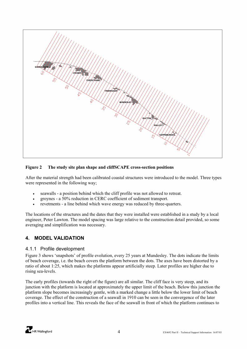
Figure 2 The study site plan shape and cliffSCAPE cross-section positions

After the material strength had been calibrated coastal structures were introduced to the model. Three typeswere represented in the following way;

� seawalls - a position behind which the cliff profile was not allowed to retreat.� groynes - a 50% reduction in CERC coefficient of sediment transport.� revetments - a line behind which wave energy was reduced by three-quarters.

The locations of the structures and the dates that they were installed were established in a study by a localengineer, Peter Lawton. The model spacing was large relative to the construction detail provided, so someaveraging and simplification was necessary.

4. MODEL VALIDATION

4.1.1 Profile developmentFigure 3 shows ‘snapshots’ of profile evolution, every 25 years at Mundesley. The dots indicate the limitsof beach coverage, i.e. the beach covers the platform between the dots. The axes have been distorted by aratio of about 1:25, which makes the platforms appear artificially steep. Later profiles are higher due torising sea-levels.

The early profiles (towards the right of the figure) are all similar. The cliff face is very steep, and itsjunction with the platform is located at approximately the upper limit of the beach. Below this junction theplatform slope becomes increasingly gentle, with a marked change a little below the lower limit of beachcoverage. The effect of the construction of a seawall in 1910 can be seen in the convergence of the laterprofiles into a vertical line. This reveals the face of the seawall in front of which the platform continues to


drop. The continuing lowering of the platform represents an increase in the vulnerability of the seawall andthe cliff it protects.

Figure 3 Model profile evolution at Mundesley, 25 year stages from 1600 to 2000

Most of the later profiles show much wider beaches, the largest being about 300 m, indicating an increasein the volume of the beach. This probably results from both the construction of groynes at this location andincreased updrift recession between Mundesley and Overstrand.

The last profile represents the present day situation and has been compared to measurements. It was foundthat the platform level close to the seawall was well represented, but the gradient is too shallow in themodel. Consequently the rest of the platform is too high. Site investigations reveal that at 30 m from thewall the platform is about 0.5 m deeper than is predicted in the model. This misrepresentation of theplatform elevation seems to be a general problem along the model coast, although data describing theactual platform is very scarce. This is a disappointing aspect of the simplistic representation of cross-shoreprocesses.

Although greater accuracy in the prediction of the platform level is desirable, it is not necessarily critical tomodel performance. The primary need is for the model to be capable of predicting planshape evolution.

4.1.2 Plan shape developmentModel planshape evolution was compared to the historic development of the North Norfolk coast, asmeasured by Cambers (1976).

6650 6700 6750 6800 6850 6900 6950 7000-3

-2

-1

0

1

2

3

4

Ele

vatio

n, m

etre

s A

OD

Distance from baseline, metres

ProfileBeach limit


Figure 4 Comparison between model recession rates and measurements provided by Cambers

The comparison, which is shown in Figure 4 is made over three eras, 1880 – 1905, 1905 – 1946 & 1946 –1967. There is some asynchrony between the model output and the historic measurement period for eras 2and 3 since data was output from the model at 5 year intervals, e.g. era 2 last from 1905 to 1945. The dotson the line for predictions each represent a model section. The results are good, both in terms of magnitudeand temporal and spatial variation. The fit is least good in era three, which is disappointing since this is themost recent. The cause is not clear but it can be attributed, in part, to the short duration of this era, (21years) and some asynchrony between the recession periods (1946-1967 measured and 1945-1970modelled). In addition there is an anomaly in the measured data at Overstrand (Chainage 21 km). Aseawall has been present there since 1920, but the measured recession over the period 1946 – 1967 is givenas approximately 0.7 m/A. The measured data also shows high recession south of Mundesley in the thirdera that contradicts local knowledge.

Although the comparison is good for the primary area of interest, from Overstrand to Mundesley, lessconfidence is established in the representation of the south of the region. The cause of this is uncertain,although it can be attributed in part to the proximity of the southern boundary and the use of only one wavepoint. The problem is also compounded by the lack of reliable calibration data south of Mundesley after1946. However, it is also the case that any misrepresentation of any area of the model will be propagateddowndrift. Since the southern area is downdrift of the rest of the model it is likely to show the largesterrors.

The good match obtained over the main part of the region lends confidence in the model performance andprovides a good basis for making future predictions.

0 1 20

5

10

15

20

25

30

35Era 1

Mod

el b

asel

ine

chai

nage

, km

0 1 20

5

10

15

20

25

30

35Era 2

Recession rate (m/A)

MeasuredModelled

0 1 20

5

10

15

20

25

30

35Era 3

H

B

M

T

O

C

S


4.2 5Scenario testingA total of 19 future management scenarios were modelled, which are summarised in Table 2. These wereused to explore the implications of structure failure, removal, maintenance and improvement and differentrates of sea-level rise. Groyne removal, damage and improvement was represented within the model byvarying the CERC coefficient, and therefore sediment transport rate, e.g. 20% model groyne damage wasrepresented by a 20% decrease in its effect on the sediment transport rate. The rate of sea-level rise post-2002 assumed for all scenarios, except Scenarios 6a-6d, was 6 mm/A.

Table 2 Summary of scenarios

No. Management scenario Notes1 Open Coast Remove all seawalls and groynes in January 20032 Do Nothing Structures removed at the mean estimate of residual life

3 SMP policy optionsSMP policy option, groynes and seawalls held in presentalignment & condition

4 Revised SMP policy options As scenario 3 but Do Nothing at Trimingham

5aSMP policy options with groynemodification 20 % increase in groyne efficiency at C, O, T, M & B

5bSMP policy options with groynemodification 20 % increase in groyne efficiency at C, O, M & B

5cSMP policy options with groynemodification 20 % increase in groyne efficiency at C, M & B

5dSMP policy options with groynemodification 20 % increase in groyne efficiency at C and B

5eSMP policy options with groynemodification 20 % increase in groyne efficiency at C

6a Do nothing 4 mm/A Sea-level rise6b SMP policy options 4 mm/A Sea-level rise6c Do nothing 2 mm/A Sea-level rise6d SMP policy options 2 mm/A Sea-level rise7a Do nothing Minimum residual life estimate7c Do nothing Maximum residual life estimate

8aSMP policy options with groynemodification

Groyne efficiency reduced by 20% at O, T, M & B,increased by 20% at C

8bSMP policy options with groynemodification

Groyne efficiency reduced by 20% at T increased by 20%at C


Groyne efficiency increased by 40% at O, T, M & B,increased by 20% at C


Groyne efficiency increased by 40% at O & M, increasedby 20% at C

N.B. C, O, T, M & B refer to Cromer, Overstrand, Trimingham, Mundesley and Bacton respectively.

The models provide cliff toe position every year at every section. These were processed to providerecession distance and average recession rate for each scenario. A full set of results is given in Appendix 1.Key representative results are described below.

4.2.1 Scenario 1, ‘Open coast’The first scenario to be tested was ‘Open Coast’ in which all model structures were removed at thebeginning of 2003. Historically these structures have resulted in the formation of anthropogenic headlands.Removal of the structures might be expected to result in the rapid removal of these features. A benefit ofreleasing the coast in this way would be the resulting supply of large amounts of sediment from the cliff tothe beach. The modelled consequences of the ‘Open Coast’ scenario are shown in Figure 5.


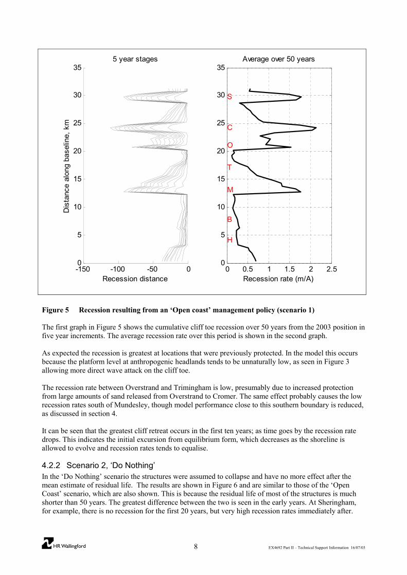
Figure 5 Recession resulting from an ‘Open coast’ management policy (scenario 1)

The first graph in Figure 5 shows the cumulative cliff toe recession over 50 years from the 2003 position infive year increments. The average recession rate over this period is shown in the second graph.

As expected the recession is greatest at locations that were previously protected. In the model this occursbecause the platform level at anthropogenic headlands tends to be unnaturally low, as seen in Figure 3allowing more direct wave attack on the cliff toe.

The recession rate between Overstrand and Trimingham is low, presumably due to increased protectionfrom large amounts of sand released from Overstrand to Cromer. The same effect probably causes the lowrecession rates south of Mundesley, though model performance close to this southern boundary is reduced,as discussed in section 4.

It can be seen that the greatest cliff retreat occurs in the first ten years; as time goes by the recession ratedrops. This indicates the initial excursion from equilibrium form, which decreases as the shoreline isallowed to evolve and recession rates tends to equalise.

4.2.2 Scenario 2, ‘Do Nothing’In the ‘Do Nothing’ scenario the structures were assumed to collapse and have no more effect after themean estimate of residual life. The results are shown in Figure 6 and are similar to those of the ‘OpenCoast’ scenario, which are also shown. This is because the residual life of most of the structures is muchshorter than 50 years. The greatest difference between the two is seen in the early years. At Sheringham,for example, there is no recession for the first 20 years, but very high recession rates immediately after.

-150 -100 -50 00

5

10

15

20

25

30

355 year stages

Recession distance

Dis

tanc

e al

ong

base

line,

km

0 0.5 1 1.5 2 2.50

5

10

15

20

25

30

35Average over 50 years


H

B

M

T

O

C

S


Figure 6 Recession resulting from a 'Do Nothing' management policy (scenario 2)

4.2.3 Scenario 3, ‘SMP policy options’The ‘SMP policy options’ scenario assumed a continuation of current management practice under whichstructures are maintained. The expected result of this policy is that the settlements would continue toemerge from the cliff line as anthropogenc headlands, separated by bays. The results of this scenario areshown in Figure 7. There are areas between Sheringham and Cromer and Overstrand and Triminghamwhere the recession rate under the ‘Do Nothing’ scenario is greater than the ‘Open Coast’ scenario. Thisprobably reflects increased protection resulting from the greater volumes of beach sediment released by thelatter scenario.

-150 -100 -50 00

5

10

15

20

25

30

355 year stages

Recession distance

Dis

tanc

e al

ong

base

line,

km

0 0.5 1 1.5 2 2.50

5

10

15

20

25

30



H

B

M

T

O

C

S

Do NothingOpen Coast


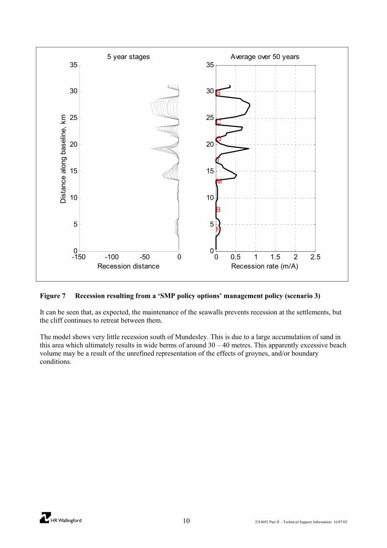
Figure 7 Recession resulting from a ‘SMP policy options’ management policy (scenario 3)

It can be seen that, as expected, the maintenance of the seawalls prevents recession at the settlements, butthe cliff continues to retreat between them.

The model shows very little recession south of Mundesley. This is due to a large accumulation of sand inthis area which ultimately results in wide berms of around 30 – 40 metres. This apparently excessive beachvolume may be a result of the unrefined representation of the effects of groynes, and/or boundaryconditions.

-150 -100 -50 00

5

10

15

20

25

30

355 year stages

Recession distance

Dis

tanc

e al

ong

base

line,

km

0 0.5 1 1.5 2 2.50

5

10

15

20

25

30



H

B

M

T

O

C

S


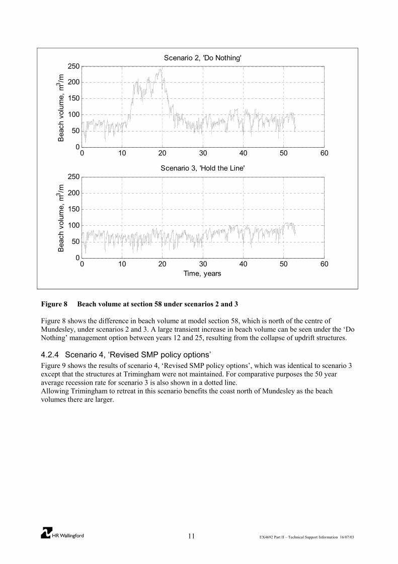
Figure 8 Beach volume at section 58 under scenarios 2 and 3

Figure 8 shows the difference in beach volume at model section 58, which is north of the centre ofMundesley, under scenarios 2 and 3. A large transient increase in beach volume can be seen under the ‘DoNothing’ management option between years 12 and 25, resulting from the collapse of updrift structures.

4.2.4 Scenario 4, ‘Revised SMP policy options’Figure 9 shows the results of scenario 4, ‘Revised SMP policy options’, which was identical to scenario 3except that the structures at Trimingham were not maintained. For comparative purposes the 50 yearaverage recession rate for scenario 3 is also shown in a dotted line.Allowing Trimingham to retreat in this scenario benefits the coast north of Mundesley as the beachvolumes there are larger.

0 10 20 30 40 50 600

50

100

150

200

250Scenario 2, 'Do Nothing'

Bea

ch v

olum

e, m

3 /m

0 10 20 30 40 50 600

50

100

150

200

250Scenario 3, 'Hold the Line'

Time, years

Bea

ch v

olum

e, m

3 /m


Figure 9 Recession resulting from a revised ‘SMP policy options’ management policy (scenario 4)

4.2.5 Scenarios 5a – 5e, ‘SMP policy options with Groyne Modification’In scenarios 5a to 5e the effect of improving groyne performance was explored. Improved groynes mightbe expected to increase the level of protection of the local cliffs but promote recession of downdrift areas.This behaviour was observed in the model results, as shown in Figure 10.

-150 -100 -50 00

5

10

15

20

25

30

355 year stages

Recession distance

Dis

tanc

e al

ong

base

line,

km

0 0.5 1 1.5 2 2.50

5

10

15

20

25

30



Dis

tanc

e al

ong

base

line,

km

H

B

M

T

O

C

S

OriginalRevised


Figure 10 Results of scenarios 3 and 5a to 5d, 'SMP policy options with groyne modifications', ‘GI’indicates a location of groyne improvement.

0 0.5 1 1.50

5

10

15

20

25

30

35(a)

Recession rate, 50A average (m/A)

Dis

tanc

e al

ong

base

line

(km

)

H

B

M

T

O

C

S

GI(5a)

GI(5a)

GI(5a)

GI(5a)

GI(5a)

GI(5b)

GI(5b)

GI(5b)

GI(5b)

Scenario 5aScenario 5bScenario 3

0 0.5 1 1.50

5

10

15

20

25

30

35(b)


Dis

tanc

e al

ong

base

line

(km

)

H

B

M

T

O

C

S

GI(5b)

GI(5b)

GI(5b)

GI(5b)

GI(5c)

GI(5c)

GI(5c)

Scenario 5bScenario 5cScenario 3

0 0.5 1 1.50

5

10

15

20

25

30

35(c)


Dis

tanc

e al

ong

base

line

(km

)

H

B

M

T

O

C

S

GI(5c)

GI(5c)

GI(5c)

GI(5d)

GI(5d)

Scenario 5cScenario 5dScenario 3

0 0.5 1 1.50

5

10

15

20

25

30

35


Dis

tanc

e al

ong

base

line

(km

)

H

B

M

T

O

C

S

GI(5d)

GI(5d)

(d)

GI(5e)

Scenario 5dScenario 5eScenario 3


In Figure 10 (a) to (d) the effects of different options of groyne improvement can be seen. In each casethere is a beneficial and detrimental effect of land lost to recession. For example in Figure 10 (a) thedifference in average recession rate between scenario 5a and scenario 5b is shown. These indicate groyneimprovement at Trimingham reducing updrift recession, but promoting it on the downdrift side.The impact of sediment restriction seems to be limited to a relatively short downdrift area. This seemsunrealistic, and may be indicative of the simplistic means of groyne representation.

4.3 6Sensitivity testsEight scenarios were used to explore model sensitivity to rate of sea-level rise and structure residual life.These are summarised in Table 3.

Table 3 Summary of sensitivity tests

No. Testing sensitivity to… Management option Assumptions6d Rate of sea-level rise SMP policy options 2 mm/A Sea-level rise6b Rate of sea-level rise SMP policy options 4 mm/A Sea-level rise3 Rate of sea-level rise SMP policy options 6 mm/A Sea-level rise6c Rate of sea-level rise Do nothing 2 mm/A Sea-level rise6a Rate of sea-level rise Do nothing 4 mm/A Sea-level rise

2Rate of sea-level rise &Residual life Do Nothing 6 mm/A Sea-level rise & mean residual life estimate

7a Residual life Do nothing Minimum residual life estimate7c Residual life Do nothing Maximum residual life estimate

4.3.1 Sensitivity to rate of sea-level riseSix scenarios were run to study the implications of accelerated sea-level rise, which was expected to causea significant increase on recession rates. The average recession rates predicted under these scenarios areshown in Figure 11. Two management policies were assumed, ‘SMP policy options’ and ‘Do Nothing’.Although a retreat rate was found to increase with accelerated sea-level rise the effect was small.


Figure 11 Average recession rates resulting from different rates of sea-level rise (SLR), (scenarios2, 3, 6a, 6b, 6c, & 6c).

Although this insensitivity is, at first, counterintuitive, it is reasonable. This region of coast is curved,which results in a changing angle of wave attack along the shore. The longshore sediment transport ratedepends on this angle so it also changes, becoming gradually larger with distance from Sheringham. Thispositive gradient in sediment transport rate tends to reduce the beach volume, i.e. at any section of thiscoast more sand tends to move out towards the south than in from the north. This would result in thebeaches being totally removed, leaving behind the underlying platform, if it were not for the supply of sandfrom retreating cliffs. If left to evolve naturally the rate of sand supplied from a section of cliff would tendto be equal to the difference in net beach sediment transport rate across that section. The process by whichthis balance is maintained is simple; if the difference in sediment transport rate increases, the beachvolume drops and larger waves attack the cliff causing increased recession resulting in the release of morecliff sediments. Conversely, if the differential in sediment transport rate drops then the beach lowers moreslowly, and is able to provide more protection than it would otherwise. Consequently cliff erosion andretreat reduces and the rate of sand supply from the cliff falls.

In this description it can be seen that the retreat rate is simply an aspect of a larger system of sedimentbalancing, which is dominated by the differential sediment transport rate.

Accelerated sea-level rise can not cause a significant increase in retreat rate in such a system. If it did thenthe beaches would grow continuously from the increased cliff sediment supply since the unchangedlongshore sediment transport rates would not be washing away all the material being supplied.

0 0.5 1 1.5 2 2.50

5

10

15

20

25

30

35


Dis

tanc

e al

ong

base

line

(km

)

H

B

M

T

O

C

S

Do Nothing

0 0.5 1 1.5 2 2.50

5

10

15

20

25

30

35


Dis

tanc

e al

ong

base

line

(km

)

H

B

M

T

O

C

S

Hold the Line

2 mm/A4 mm/A6 mm/A


4.3.2 Sensitivity to residual life

Figure 12 Average recession rates resulting from three ‘Do nothing’ management options, withdifferent estimates of residual life (RL) (scenarios 2, 7a & 7c).

Figure 12 shows results from three ‘Do nothing’ scenarios, in which sensitivity to estimated residual life(RL) was explored. The 50 year average recession rate does vary with the different choices of residual life,though the relationship is not strong. This is, in part, due to the relatively small residual life of thestructures (average of 6.7 years) and the smaller difference between the maxima and minima (average of2.3 years). Despite this it can be seen that, as expected, the lower estimate of residual life results in moreerosion of the anthropogenic headlands than the higher estimate. However, towards the southern boundaryof the model, in the Happisburgh area, the trend is reversed. This is probably due to differences in thebeach volumes at Happisburgh under the different scenarios, i.e. less residual life leads to more recessionand greater quantities of sand released into the system. However, as was discussed in section 4, confidenceis model behaviour south of Mundesley is reduced.

0 0.5 1 1.5 2 2.50

5

10

15

20

25

30

35


Dis

tanc

e al

ong

base

line

(km

)

H

B

M

T

O

C

S

Minimum RLMean RLMaximum RL


�s �i�f

Cliff top

Clifftoe

Pre-landslide

slope

Post-landslide

slopeNext pre-landslideslope

Cross-shore distance

Initial cliff toeposition, xb,i

Initial cliff topposition, xc,i

Cliff top recession distanceduring previous landslide

x

Cliffheight, h

5. A STOCHASTIC MODEL OF COASTAL CLIFF LANDSLIDING

For economic appraisal of the impacts of coastal cliff recession, predictions are required of whenindividual cliff-top assets will be lost due to coastal landsliding. Coastal landsliding is a consequence of acombination of cliff toe recession and geotechnical processes within the cliff slope. On the north Norfolkcoast landsliding on unprotected coasts proceeds by a process of marine removal of material from the clifftoe, resulting in steepening the coastal slope. Eventually the slope becomes geotechnically unstable and alandslide occurs, which reduced the coastal slope and delivers debris to the beach. The timing of thelandslide is a function of the rate of removal of material from the cliff toe and other processes, primarilyconnected with pore pressure distributions within the cliff, that influence cliff stability. The timing of alandslide cannot be predicted precisely. However, knowledge of the rate of shoreline retreat (fromcliffSCAPE) can be combined with an assessment of the geotechnical characteristics of the slope togenerate an approximate prediction of cliff top location (Walkden et al. 2002).

The approach adopted here is based on the notion of a Cliff Behavioural Unit (CBU) as being a stretch ofcliff-line which behaves in broadly the same way. Within a CBU, the cliff can be expected to fail when itreaches a average angle �f and will, after failure, adopt an angle �s. Of course neither �f nor �s can bepredicted precisely. They will vary because of temporal variations in pore pressure and local variations incliff strength and composition. Even if all the required information were available, they could still not bepredicted precisely because of uncertainties in our understanding of the processes of coastal landsliding.This uncertainty in �f and �s has been included in the analysis by representing both values as Normallydistributed random variables, with means and variances obtained from geomorphological assessment of theCBU. The situation is illustrated diagrammatically in Figure 13.

Figure 13 Diagrammatic representation of the coastal landsliding model

Further uncertainty is apparent in the initial cliff angle at the site. Within a CBU there will be a range ofinitial angles, whilst in this analysis (other than for very long CBUs) a prediction of cliff top recession hasbeen generated for entire CBUs or, where appropriate, sub-sections thereof. The initial cliff angle has


therefore also been represented as a Normally distributed random variable, with mean and variance basedon measurements of cliff angle within the CBU.

From Figure 13 we see that the distance the cliff toe has to retreat until the first landslide is h(cot�i - cot�f)and the distance lost between each subsequent landslide to the next is h(cot�s - cot�f). It is thereforestraightforward to simulate the cliff top recession process, given

� cliffSCAPE predictions of cliff toe recession,� the cliff height,� the initial cliff angle �i ~ N(�i, �i), i.e. is a Normally distributed random variable with mean �i and

standard deviation �i, and� geomorphological assessments of the pre and post landslide angles �f ~ N(�f, �f), �s ~ N(�s, �s).

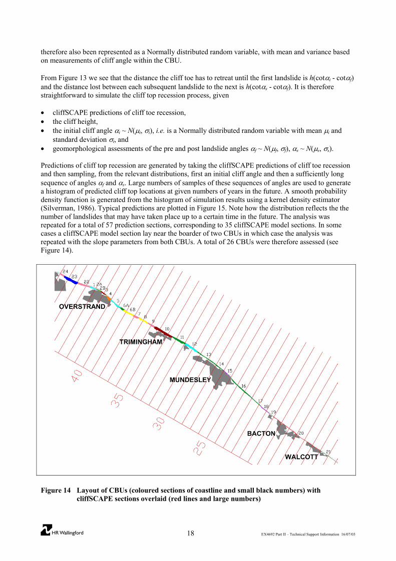
Predictions of cliff top recession are generated by taking the cliffSCAPE predictions of cliff toe recessionand then sampling, from the relevant distributions, first an initial cliff angle and then a sufficiently longsequence of angles �f and �s. Large numbers of samples of these sequences of angles are used to generatea histogram of predicted cliff top locations at given numbers of years in the future. A smooth probabilitydensity function is generated from the histogram of simulation results using a kernel density estimator(Silverman, 1986). Typical predictions are plotted in Figure 15. Note how the distribution reflects the thenumber of landslides that may have taken place up to a certain time in the future. The analysis wasrepeated for a total of 57 prediction sections, corresponding to 35 cliffSCAPE model sections. In somecases a cliffSCAPE model section lay near the boarder of two CBUs in which case the analysis wasrepeated with the slope parameters from both CBUs. A total of 26 CBUs were therefore assessed (seeFigure 14).

Figure 14 Layout of CBUs (coloured sections of coastline and small black numbers) withcliffSCAPE sections overlaid (red lines and large numbers)


Table 4 Cliff top recession prediction input data

Height, E(�i) Var(�i) E(�s) Var(�s) E(�f) Var(�f) cliffSCAPE8 40 51 48 7 32 3 136 42 25 48 7 32 3 146 60 0.1 41 4 31 2 145 60 0.1 41 4 31 2 155 60 0.1 41 4 31 2 165 60 0.1 41 4 31 2 174 60 0.1 41 4 31 2 184 60 0.1 41 4 31 2 196 60 0.1 41 4 31 2 206 32 2 34 1 30 1 208 32 2 34 1 30 1 218 29 1 29 1 38 1 21

12 30 1 29 1 38 1 2217 48 6 50 5 45 1 2217 40 20 39 4 31 3 2225 37 20 39 4 31 3 2325 39 1 39 4 31 3 2425 41 1 39 4 31 3 2519 36 16 39 4 31 3 2613 37 0.1 37 1 33 1 2613 37 0.1 37 1 33 1 2713 35 11 40 1 35 1 2723 37 11 40 1 35 1 2833 41 1 43 3 36 2 2936 37 12 43 3 36 2 3036 28 4 30 1 25 1 3040 28 4 30 1 25 1 3150 30 4 30 1 25 1 3250 33 6 33 3 30 1 3260 38 22 33 3 30 1 3360 22 6 25 1 20 1 3355 22 6 25 1 20 1 3450 23 6 25 1 20 1 3550 23 6 25 1 20 1 3644 28 31 35 2 20 1 3637 38 6 40 3 35 2 3637 38 6 40 3 35 2 3745 27 64 38 4 20 1 3845 35 0.1 40 3 34 2 3853 35 0.1 40 3 34 2 3953 40 12 40 3 34 2 3942 37 12 40 3 34 2 4042 32 39 43 4 25 1 4030 30 17 43 4 25 1 4130 19 24 30 2 18 4 4125 20 24 30 2 18 4 4225 29 4 30 2 25 1 4225 30 4 30 2 37 2 4220 30 4 30 2 37 2 4320 41 1 40 3 37 2 4320 28 6 33 4 23 1 4320 23 6 33 4 23 1 4443 25 8 29 1 24 1 4465 30 8 29 1 24 1 4565 22 4 28 2 21 1 4547 31 28 28 2 21 1 4629 33 5 33 1 30 1 47


0 5 10 15 20 25 30 35 400

0.02

0.04

0.06

0.08

0.1

0.12

0.14

0.16

0.18

0.2

Distance from 2003 cliff toe

Pro

babi

lity

dens

ity

year 10year 20year 30year 40year 50

Figure 15 Typical cliff top recession predictions (cliffSCAPE section 13 in Scenario 1)

Initial clifftop

location


6. CONCLUSIONS

This report represents the output from the first application of cliffSCAPE-RS, a regional modelling tool forsoft cliff shorelines. The results of the validation process are very positive. A good match was foundbetween model output and historic records of shore recession over three eras spanning a total of 87 years.This comparison is particularly encouraging because the measured recession rates are highly variable inboth space and time. The match was less good towards the south of the model. It is surprising andinformative that a good match was achieved with historic recession rates with minimal variation of thematerial strength parameter (R). Appropriate recession rates emerged by representing structure installation.This lends support to the manner in which there structures were represented and implies that the erosion ofthe North Norfolk cliffs is not dominated by material strength, but by management practice and it’s effecton sediment transport rates. However the results of scenarios 5a to 5e indicate that the way in which thegroynes were represented (as a reduction in the CERC coefficient of longshore transport) may have beentoo simplistic. Should another model of this coast be developed this aspect should be revisited. Inparticular it may be beneficial to represent sand bypassing when beaches become sufficiently full.

Despite the encouraging performance of the model, the reader should be aware that cliffSCAPE has onlypreviously been applied at one other coastal site (the Naze on the Essex coast) and has never previouslybeen applied to a length of coastline tested in this study. The results are therefore somewhat experimental.CliffSCAPE still requires testing and validation on a wider range of coastal sites. Because the techniqueused is novel the results should, as with any model predictions, be interpreted and utilised with somecaution. It should also be noted that the future scenarios rely on conditions that have not appeared, at leastexplicitly, in the historic record; a change in the rate of sea-level rise and the removal of protectivestructures. This is a fundamental aspect of the problem of making predictions of the Norfolk coast whichwould promote uncertainty in results regardless of the technique employed to obtain them. However,cliffSCAPE is a process-based modelling tool, so is designed to deal with this type of situation.

The dependence of the recession on sediment transport explains the observation of the relative insensitivityof the system to changes in rate of sea-level rise. Rising sea-levels have little direct influence on rates ofsediment transport.

CliffSCAPE-RS has been successfully used to model the historic development of the North Norfolk coast,and to predict future changes under a range of management scenarios. The models have developedunderstanding of the cliff system as one which is strongly influenced by sediment transport rate, withrecession rates in particular areas strongly dependent on both current and historic management decisionsboth locally and up-drift.


7. REFERENCES

Cambers, G. 1976 Temporal Scales in Coastal Erosion Systems. Transactions of the Institute of BristishGeographers. (1), 246-256.

Ferreira, O., Ciavola, P., Taborda, R., Bairros, M. and Dias, J.A. 2000. Sediment Mixing DepthDetermination for Steep and Gentle Foreshores. Journal of Coastal Research, 16(3), 830-839.

Kamphuis, J.W. 1987. Recession Rates of Glacial Till Bluffs. Journal of Waterway, Port, Coastal andOcean Engineering, 113(1), 60-73.

McDougal, W.G., and Hudspeth, R.T., 1984. Longshore Sediment Transport on Dean Beach Profiles.Proc. 19th International Conference on Coastal Engineering, Huston, USA, Vol. II, Ch. 101, 1488-1506.

Shore Protection Manual 1984, Coastal Engineering Research Centre, Waterways Experiment Station,Vicksburg, USA.

Silverman, B.W., 1986. Density Estimation for Statistics and Data Analysis. Chapman and Hall, NewYork.

Skafel, M.G. 1995. Laboratory Measurement of Nearshore Velocities and Erosion of Cohesive Sediment(Till) Shorelines. Technical note, Coastal Engineering, 24, 343-349.

Skafel, M.G., and Bishop, C.T. 1994. Flume experiments on the erosion of till shores by waves. CoastalEngineering 23, 329-348.

Walkden, M.J., Hall, J.W., and Lee, E.M. 2002. A modelling tool for predicting coastal cliff recessionand analysing cliff management options. Proc. Instability Planning and Management, Ventnor, Isle ofWight, May 20-23, edited by R.G. McInnes and J. Jakeways. London: Thomas Telford, pp.415-422.

�� EX4692 Part II – Technical Support Information 16/07/03

Appendix

Overstrand to Mundesley Strategy Study:cliff toe recession results


-150 -100 -50 00

5

10

15

20

25

30

355 year stages

Recession distance

Dis

tanc

e al

ong

base

line,

km

0 0.5 1 1.5 2 2.50

5

10

15

20

25

30



H

B

M

T

O

C

S

No. Management scenario Notes1 Open Coast Remove all seawalls and groynes in January 2003

-150 -100 -50 00

5

10

15

20

25

30

355 year stages

Recession distance

Dis

tanc

e al

ong

base

line,

km

0 0.5 1 1.5 2 2.50

5

10

15

20

25

30



H

B

M

T

O

C

S

No. Management scenario Notes

2 Do NothingStructures removed at the mean estimate ofresidual life


-150 -100 -50 00

5

10

15

20

25

30

355 year stages

Recession distance

Dis

tanc

e al

ong

base

line,

km

0 0.5 1 1.5 2 2.50

5

10

15

20

25

30



H

B

M

T

O

C

S


3 SMP policy optionsSMP policy option, groynes and seawalls held inpresent alignment & condition

-150 -100 -50 00

5

10

15

20

25

30

355 year stages

Recession distance

Dis

tanc

e al

ong

base

line,

km

0 0.5 1 1.5 2 2.50

5

10

15

20

25

30



H

B

M

T

O

C

S

No. Management scenario Notes4 Revised SMP policy options As scenario 3 but Do Nothing at Trimingham


-150 -100 -50 00

5

10

15

20

25

30

355 year stages

Recession distance

Dis

tanc

e al

ong

base

line,

km

0 0.5 1 1.5 2 2.50

5

10

15

20

25

30



H

B

M

T

O

C

S


5aSMP policy options with groynemodification 20 % increase in groyne efficiency at C, O, T, M & B

-150 -100 -50 00

5

10

15

20

25

30

355 year stages

Recession distance

Dis

tanc

e al

ong

base

line,

km

0 0.5 1 1.5 2 2.50

5

10

15

20

25

30



H

B

M

T

O

C

S


5bSMP policy options with groynemodification 20 % increase in groyne efficiency at C, O, M & B


-150 -100 -50 00

5

10

15

20

25

30

355 year stages

Recession distance

Dis

tanc

e al

ong

base

line,

km

0 0.5 1 1.5 2 2.50

5

10

15

20

25

30



H

B

M

T

O

C

S


5cSMP policy options with groynemodification 20 % increase in groyne efficiency at C, M & B

-150 -100 -50 00

5

10

15

20

25

30

355 year stages

Recession distance

Dis

tanc

e al

ong

base

line,

km

0 0.5 1 1.5 2 2.50

5

10

15

20

25

30



H

B

M

T

O

C

S


5dSMP policy options with groynemodification 20 % increase in groyne efficiency at C and B


-150 -100 -50 00

5

10

15

20

25

30

355 year stages

Recession distance

Dis

tanc

e al

ong

base

line,

km

0 0.5 1 1.5 2 2.50

5

10

15

20

25

30



H

B

M

T

O

C

S


5eSMP policy options with groynemodification 20 % increase in groyne efficiency at C

-150 -100 -50 00

5

10

15

20

25

30

355 year stages

Recession distance

Dis

tanc

e al

ong

base

line,

km

0 0.5 1 1.5 2 2.50

5

10

15

20

25

30



H

B

M

T

O

C

S

No. Management scenario Notes6a Do nothing 4 mm/A Sea-level rise


-150 -100 -50 00

5

10

15

20

25

30

355 year stages

Recession distance

Dis

tanc

e al

ong

base

line,

km

0 0.5 1 1.5 2 2.50

5

10

15

20

25

30



H

B

M

T

O

C

S

No. Management scenario Notes6b SMP policy options 4 mm/A Sea-level rise

-150 -100 -50 00

5

10

15

20

25

30

355 year stages

Recession distance

Dis

tanc

e al

ong

base

line,

km

0 0.5 1 1.5 2 2.50

5

10

15

20

25

30



H

B

M

T

O

C

S

No. Management scenario Notes6c Do nothing 2 mm/A Sea-level rise


-150 -100 -50 00

5

10

15

20

25

30

355 year stages

Recession distance

Dis

tanc

e al

ong

base

line,

km

0 0.5 1 1.5 2 2.50

5

10

15

20

25

30



H

B

M

T

O

C

S

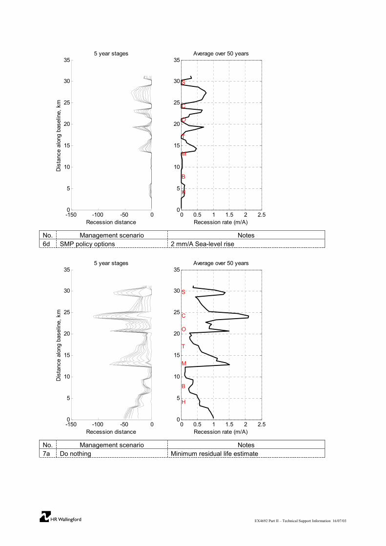
No. Management scenario Notes6d SMP policy options 2 mm/A Sea-level rise

-150 -100 -50 00

5

10

15

20

25

30

355 year stages

Recession distance

Dis

tanc

e al

ong

base

line,

km

0 0.5 1 1.5 2 2.50

5

10

15

20

25

30



H

B

M

T

O

C

S

No. Management scenario Notes7a Do nothing Minimum residual life estimate


-150 -100 -50 00

5

10

15

20

25

30

355 year stages

Recession distance

Dis

tanc

e al

ong

base

line,

km

0 0.5 1 1.5 2 2.50

5

10

15

20

25

30



H

B

M

T

O

C

S

No. Management scenario Notes7c Do nothing Maximum residual life estimate

-150 -100 -50 00

5

10

15

20

25

30

355 year stages

Recession distance

Dis

tanc

e al

ong

base

line,

km

0 0.5 1 1.5 2 2.50

5

10

15

20

25

30



H

B

M

T

O

C

S



Groyne efficiency reduced by 20% at O, T, M & B,increased by 20% at C


-150 -100 -50 00

5

10

15

20

25

30

355 year stages

Recession distance

Dis

tanc

e al

ong

base

line,

km

0 0.5 1 1.5 2 2.50

5

10

15

20

25

30



H

B

M

T

O

C

S



Groyne efficiency reduced by 20% at T increased by20% at C

-150 -100 -50 00

5

10

15

20

25

30

355 year stages

Recession distance

Dis

tanc

e al

ong

base

line,

km

0 0.5 1 1.5 2 2.50

5

10

15

20

25

30



H

B

M

T

O

C

S



Groyne efficiency increased by 40% at O, T, M & B,increased by 20% at C


-150 -100 -50 00

5

10

15

20

25

30

355 year stages

Recession distance

Dis

tanc

e al

ong

base

line,

km

0 0.5 1 1.5 2 2.50

5

10

15

20

25

30



H

B

M

T

O

C

S



Groyne efficiency increased by 40% at O & M,increased by 20% at C

overstrand to walcott strategy study - north norfolk · overstrand to walcott strategy study ......

Documents