Oversampling for Imbalanced Learning

Based on K-Means and SMOTE

Felix Last1,*, Georgios Douzas1, and Fernando Bacao1

1NOVA Information Management School, Universidade Nova de Lisboa

*Corresponding author: mail@felixlast.de

Postal Address: NOVA Information Management School, Campus de Campolide, 1070-312 Lisboa, PortugalTelephone: +351 21 382 8610

Abstract

Learning from class-imbalanced data continues to be a common and challenging problem in su-pervised learning as standard classification algorithms are designed to handle balanced class distribu-tions. While different strategies exist to tackle this problem, methods which generate artificial datato achieve a balanced class distribution are more versatile than modifications to the classificationalgorithm. Such techniques, called oversamplers, modify the training data, allowing any classifierto be used with class-imbalanced datasets. Many algorithms have been proposed for this task, butmost are complex and tend to generate unnecessary noise. This work presents a simple and effectiveoversampling method based on k-means clustering and SMOTE oversampling, which avoids the gen-eration of noise and effectively overcomes imbalances between and within classes. Empirical resultsof extensive experiments with 71 datasets show that training data oversampled with the proposedmethod improves classification results. Moreover, k-means SMOTE consistently outperforms otherpopular oversampling methods. An implementation is made available in the python programminglanguage.

1 Introduction

The class imbalance problem in machine learning describes classification tasks in which classes of data arenot equally represented. In many real-world applications, the nature of the problem implies a sometimesheavy skew in the class distribution of a binary or multi-class classification problem. Such applicationsinclude fraud detection in banking, rare medical diagnoses, and oil spill recognition in satellite images,all of which naturally exhibit a minority class (Chawla et al., 2002; Kotsiantis et al., 2006, 2007; Galaret al., 2012).

The predictive capability of classification algorithms is impaired by class imbalance. Many such algo-rithms aim at maximizing classification accuracy, a measure which is biased towards the majority class.A classifier can achieve high classification accuracy even when it does not predict a single minority classinstance correctly. For example, a trivial classifier which scores all credit card transactions as legit willscore a classification accuracy of 99.9% assuming that 0.1% of transactions are fraudulent; however inthis case, all fraud cases remain undetected. In conclusion, by optimizing classification accuracy, mostalgorithms assume a balanced class distribution (Provost, 2000; Kotsiantis et al., 2007).

Another inherent assumption of many classification algorithms is the uniformity of misclassification costs,which is rarely a characteristic of real-world problems. Typically in imbalanced datasets, misclassifyingthe minority class as the majority class has a higher cost associated with it than vice versa. An exampleof this is database marketing, where the cost of mailing to a non-respondent is much lower than the lostprofit of not mailing to a respondent (Domingos, 1999).

Lastly, what is referred to as the “small disjuncts problem” is often encountered in imbalanced datasets (Galaret al., 2012). The problem refers to classification rules covering only a small number of training examples.The presence of only few samples make rule induction more susceptible to error (Holte et al., 1989). Toillustrate the importance of discovering high quality rules for sparse areas of the input space, the example

1

arX

iv:1

711.

0083

7v2

[cs

.LG

] 1

2 D

ec 2

017

of credit card fraud detection is again considered. Assume that most fraudulent transactions are pro-cessed outside the card owner’s home country. The remaining cases of fraud happen within the country,but show some different exceptional characteristic, such as a high amount, an unusual time or recurringcharges. Each of these other characteristics applies to only a very small group of transactions, which byitself is often vanishingly small. However, adding up all these edge cases, they can make up a substantialportion of all fraudulent transactions. Therefore, it is important that classifiers pay adequate attentionto small disjuncts (Holte et al., 1989).

Techniques aimed at improving classification in the presence of class imbalance can be divided into threebroad categories1: algorithm level methods, data level methods, and cost-sensitive methods.

Solutions which modify the classification algorithm to cope with the imbalance are algorithm level tech-niques (Kotsiantis et al., 2006; Galar et al., 2012). Such techniques include changing the decision thresh-old and training separate classifiers for each class (Kotsiantis et al., 2006; Chawla et al., 2004).

In contrast, cost-sensitive methods aim at providing classification algorithms with different misclassifica-tion costs for each class. This requires knowledge of misclassification costs, which are dataset-dependentand commonly unknown or difficult to quantify. Additionally, the algorithms must be capable of in-corporating the misclassification cost of each class or instance into their optimization. Therefore, thesemethods are regarded as operating both on data and algorithm level (Galar et al., 2012).

Finally, data-level methods manipulate the training data, aiming to change the class distribution to-wards a more balanced one. Techniques in this category resample the data by removing cases of themajority classes (undersampling) or adding instances to the minority classes by means of duplication orgeneration of new samples (oversampling) (Kotsiantis et al., 2006; Galar et al., 2012). Because under-sampling removes data, such methods risk the loss of important concepts. Moreover, when the numberof minority observations is small, undersampling to a balanced distribution yields an undersized dataset,which may in turn limit classifier performance. Oversampling, on the other hand, may encourage over-fitting when observations are merely duplicated (Weiss et al., 2007). This problem can be avoided byadding genuinely new samples. One straightforward approach to this is synthetic minority over-samplingtechnique (SMOTE), which interpolates existing samples to generate new instances.

Data-level methods can be further discriminated into random and informed methods. Unlike randommethods, which randomly choose samples to be removed or duplicated (e.g. Random Oversampling,SMOTE), informed methods take into account the distribution of the samples (Chawla et al., 2004).This allows informed methods to direct their efforts to critical areas of the input space, for instance tosparse areas (Nickerson et al., 2001), safe areas (Bunkhumpornpat et al., 2009), or to areas close to thedecision boundary (Han et al., 2005). Consequently, informed methods may avoid the generation of noiseand can tackle imbalances within classes.

Unlike algorithm-level methods, which are bound to a specific classifier, and cost-sensitive methods,which are problem-specific and need to be implemented by the classifier, data-level methods can beuniversally applied and are therefore more versatile (Galar et al., 2012).

Many oversampling techniques have proven to be effective in real-world domains. SMOTE is the mostpopular oversampling method that was proposed to improve random oversampling. There are multiplevariations of SMOTE which aim to combat the original algorithm’s weaknesses. Yet, many of theseapproaches are either very complex or alleviate only one of SMOTE’s shortcomings. Additionally, fewof them are readily available in a unified software framework used by practitioners.

This paper suggests the combination of the k-means clustering algorithm in combination with SMOTE tocombat some of other oversampler’s shortcomings with a simple-to-use technique. The use of clusteringenables the proposed oversampler to identify and target areas of the input space where the generationof artificial data is most effective. The method aims at eliminating both between-class imbalances andwithin-class imbalances while at the same time avoiding the generation of noisy samples. Its appeal is thewidespread availability of both underlying algorithms as well the effectiveness of the method itself.

While the proposed method could easily be extended to cope with multi-class problems, the focus ofthis work is placed on binary classification tasks. When working with more than two imbalanced classes,

1The three categories are not exhaustive and new categories have been introduced, such as the combination of each ofthese techniques with ensemble learning (Galar et al., 2012).

2

different aspects of classification, as well as evaluation, must be considered, which is discussed in detailby Fernandez et al. (2013).

The remainder of this work is organized as follows. In section 2, related work is summarized and currentlyavailable oversampling methods are introduced. Special attention is paid to oversamplers which - likethe proposed method - employ a clustering procedure. Section 3 explains in detail how the proposedoversampling technique works and which hyperparameters need to be tuned. It is shown that bothSMOTE and random oversampling are limit cases of the algorithm and how they can be achieved. Insection 4, a framework aimed at evaluating the performance of the proposed method in comparison withother oversampling techniques is established. The experimental results are shown in section 5, which isfollowed by section 6 presenting the conclusions.

2 Related Work

Methods to cope with class imbalance either alter the classification algorithm itself, incorporate misclas-sification costs of the different classes into the classification process, or modify the data used to train theclassifier. Resampling the training data can be done by removing majority class samples (undersampling)or by inflating the minority class (oversampling). Oversampling techniques either duplicate existing ob-servations or generate artificial data. Such methods may work uninformed, randomly choosing sampleswhich are replicated or used as a basis for data generation, or informed, directing their efforts to areaswhere oversampling is deemed most effective. Among informed oversamplers, clustering procedures aresometimes applied to determine suitable areas for the generation of synthetic samples.

Random oversampling randomly duplicates minority class instances until the desired class distributionis reached. Due to its simplicity and ease of implementation, it is likely to be the method that is mostfrequently used among practitioners. However, since samples are merely replicated, classifiers trainedon randomly oversampled data are likely to suffer from overfitting2 (Batista et al., 2004; Chawla et al.,2004).

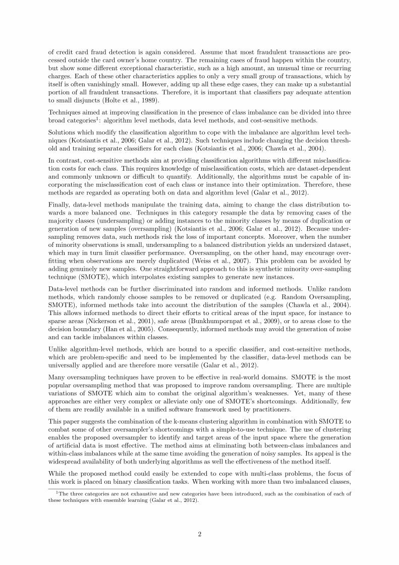
In 2002, Chawla et al. (2002) suggested the SMOTE algorithm, which avoids the risk of overfitting facedby random oversampling. Instead of merely replicating existing observations, the technique generatesartificial samples. As shown in figure 1, this is achieved by linearly interpolating a randomly selectedminority observation and one of its neighboring minority observations. More precisely, SMOTE executesthree steps to generate a synthetic sample. Firstly, it chooses a random minority observation ~a. Amongits k nearest minority class neighbors, instance ~b is selected. Finally, a new sample ~x is created byrandomly interpolating the two samples: ~x = ~a+w× (~b−~a), where w is a random weight in [0, 1].

Figure 1: SMOTE linearly interpolates a randomly selected minority sample and one of its k = 4 nearestneighbors

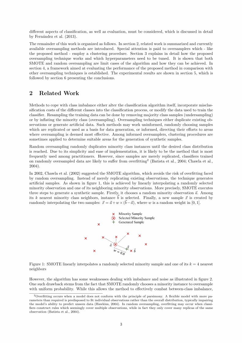
However, the algorithm has some weaknesses dealing with imbalance and noise as illustrated in figure 2.One such drawback stems from the fact that SMOTE randomly chooses a minority instance to oversamplewith uniform probability. While this allows the method to effectively combat between-class imbalance,

2Overfitting occurs when a model does not conform with the principle of parsimony. A flexible model with more pa-rameters than required is predisposed to fit individual observations rather than the overall distribution, typically impairingthe model’s ability to predict unseen data (Hawkins, 2004). In random oversampling, overfitting may occur when classi-fiers construct rules which seemingly cover multiple observations, while in fact they only cover many replicas of the sameobservation (Batista et al., 2004).

3

the issues of within-class imbalance and small disjuncts are ignored. Input areas counting many minoritysamples have a high probability of being inflated further, while sparsely populated minority areas arelikely to remain sparse (Prati et al., 2004).

Another major concern is that SMOTE may further amplify noise present in the data. This is likelyto happen when linearly interpolating a noisy minority sample, which is located among majority classinstances, and its nearest minority neighbor. The method is susceptible to noise generation because itdoesn’t distinguish overlapping class regions from so-called safe areas (Bunkhumpornpat et al., 2009).

Finally, the algorithm does not specifically enforce the decision boundary. Instances far from the classborder are oversampled with the same probability as those close to the boundary. It has been argued thatclassifiers could benefit from the generation of samples closer to the class border (Han et al., 2005).

Figure 2: Behavior of SMOTE in the presence of noise and within-class imbalance

Despite its weaknesses, SMOTE has been widely adopted by researchers and practitioners, likely dueto its simplicity and added value with respect to random oversampling. Numerous extensions of thetechnique have been developed, which aim to eliminate its disadvantages. Such extensions typicallyaddress one of the original method’s weaknesses. They may be divided according to their claimed goalinto algorithms which aim to emphasize certain minority class regions, intend to combat within-classimbalance, or attempt to avoid the generation of noise.

Focussing its attention on the decision boundary, borderline-SMOTE1 belongs to the category of methodsemphasizing class regions. It is the only algorithm discussed here which does not employ a clusteringprocedure and is included due to its popularity. The technique replaces SMOTE’s random selection ofobservations with a targeted selection of instances close to the class border. The label of a sample’sk nearest neighbors is used to determine whether it is discarded as noise, selected for its presumedproximity to the class border, or ruled out because it is far from the boundary. Borderline-SMOTE2extends this method to allow interpolation of a minority instance and one of its majority class neighbors,setting the interpolation weight to less than 0.5 so as to place the generated sample closer to the minoritysample (Han et al., 2005).

Cluster-SMOTE, another method in the category of techniques emphasizing certain class regions, usesk-means to cluster the minority class before applying SMOTE within the found clusters. The statedgoal of this method is to boost class regions by creating samples within naturally occurring clusters ofthe minority class. It is not specified how many instances are generated in each cluster, nor how theoptimal number of clusters can be determined (Cieslak et al., 2006). While the method may alleviatethe problem of between-class imbalance, it does not help to eliminate small disjuncts.

Belonging to the same category, adaptive semi-unsupervised weighted oversampling (A-SUWO) intro-duced by Nekooeimehr and Lai-Yuen (2016), is a rather complex technique which applies clustering

4

to improve the quality of oversampling. The approach is based on hierarchical clustering and aims atoversampling hard-to-learn instances close to the decision boundary.

Among techniques which aim to reduce within-class imbalance at the same time as between-class im-balance is cluster-based oversampling. The algorithm clusters the entire input space using k-means.Random oversampling is then applied within clusters so that: a) all majority clusters, b) all minorityclusters, and c) the majority and minority classes are of the same size (Jo and Japkowicz, 2004). Byreplicating observations instead of generating new ones, this technique may encourage overfitting.

With a bi-directional sampling approach, Song et al. (2016) combine undersampling the majority classwith oversampling the minority class. K-means clustering is applied separately within each class withthe goal of achieving within- and between-class balance. For clustering the majority class, the numberof clusters is set to the desired number of samples (equal to the geometric mean of instances per class).The class is undersampled by retaining only the nearest neighbor of each cluster centroid. The minorityclass is clustered into two partitions. Subsequently, SMOTE is applied in the smaller cluster. A numberof iterations of clustering and SMOTE are performed until both classes are of equal size. It is unclearhow many samples are added at each iteration. Since the method clusters both classes separately, it isblind to overlapping class borders and may contribute to noise generation.

The self-organizing map oversampling (SOMO) algorithm transforms the input data into a two-dimensionalspace using a self-organizing map, where safe and effective areas are identified for data generation.SMOTE is then applied within clusters found in the lower dimensional space, as well as between neigh-boring clusters in order to correct within- and between-class imbalances (Douzas and Bacao, 2017).

Aiming to avoid noise generation, a clustering-based approach called CURE-SMOTE uses the hierarchicalclustering algorithm CURE to clear the data of outliers before applying SMOTE. The rationale behindthis method is that because SMOTE would amplify existing noise, the data should be cleared of noisyobservations prior to oversampling (Ma and Fan, 2017). While noise generation is avoided, possibleimbalances within the minority class are ignored.

Finally, Santos et al. (2015) cluster the entire input space with k-means. Clusters with few representativesare chosen to be oversampled using SMOTE. The algorithm is different from most oversampling methodsin that SMOTE is applied regardless of the class label. The class label of the generated sample is copiedfrom the nearest of the two parents. The algorithm thereby targets dataset imbalance, rather thanimbalances between or within classes and cannot be used to solve class imbalance.

In summary, there has been a lot of recent research aimed at the improvement of imbalanced datasetresampling. Some proposed methods employ clustering techniques before applying random oversamplingor SMOTE. While most of them manage to combat some weaknesses of existing oversampling algorithms,none have been shown to avoid noise generation and alleviate imbalances both between and within classesat the same time. Additionally, many techniques achieve their respective improvements at the cost ofhigh complexity, making the techniques difficult to implement and use.

3 Proposed Method

The method proposed in this work employs the simple and popular k-means clustering algorithm inconjunction with SMOTE oversampling in order to rebalance skewed datasets. It manages to avoid thegeneration of noise by oversampling only in safe areas. Moreover, its focus is placed on both between-class imbalance and within-class imbalance, combating the small disjuncts problem by inflating sparseminority areas. The method is easily implemented due to its simplicity and the widespread availabilityof both k-means and SMOTE. It is uniquely different from related methods not only due to its lowcomplexity but also because of its effective approach to distributing synthetic samples based on clusterdensity.

3.1 Algorithm

K-means SMOTE consists of three steps: clustering, filtering, and oversampling. In the clustering step,the input space is clustered into k groups using k-means clustering. The filtering step selects clustersfor oversampling, retaining those with a high proportion of minority class samples. It then distributes

5

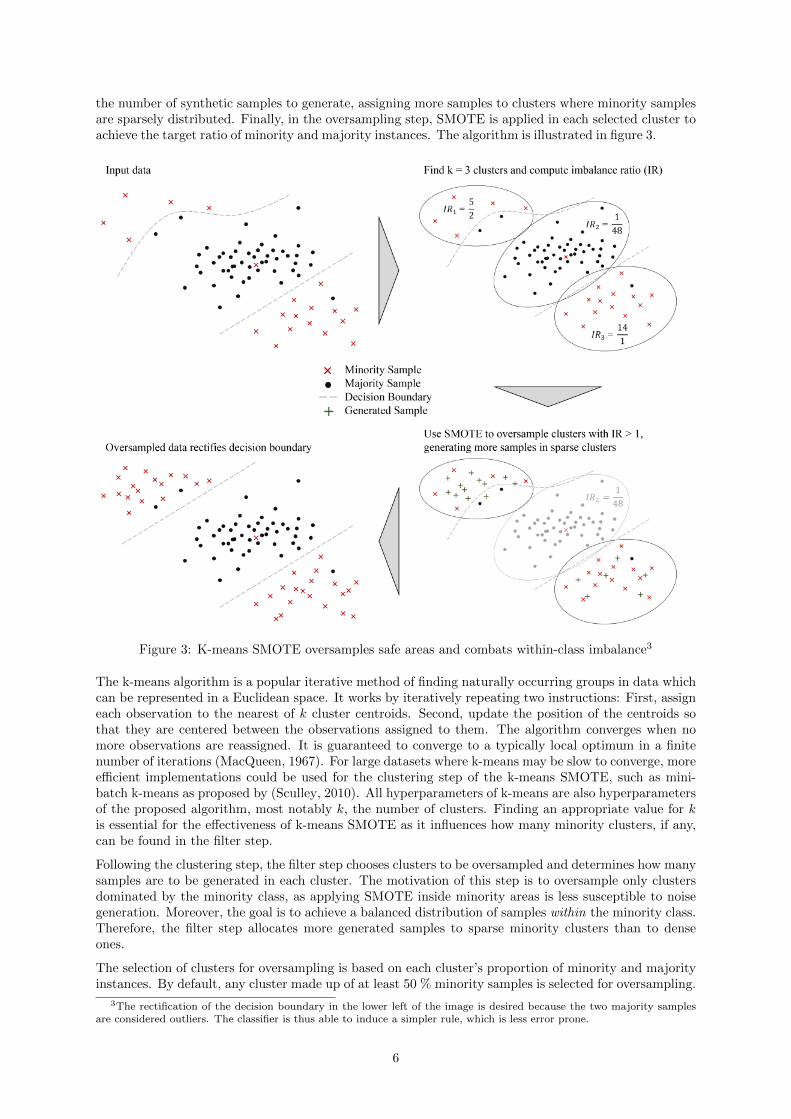
the number of synthetic samples to generate, assigning more samples to clusters where minority samplesare sparsely distributed. Finally, in the oversampling step, SMOTE is applied in each selected cluster toachieve the target ratio of minority and majority instances. The algorithm is illustrated in figure 3.

Figure 3: K-means SMOTE oversamples safe areas and combats within-class imbalance3

The k-means algorithm is a popular iterative method of finding naturally occurring groups in data whichcan be represented in a Euclidean space. It works by iteratively repeating two instructions: First, assigneach observation to the nearest of k cluster centroids. Second, update the position of the centroids sothat they are centered between the observations assigned to them. The algorithm converges when nomore observations are reassigned. It is guaranteed to converge to a typically local optimum in a finitenumber of iterations (MacQueen, 1967). For large datasets where k-means may be slow to converge, moreefficient implementations could be used for the clustering step of the k-means SMOTE, such as mini-batch k-means as proposed by (Sculley, 2010). All hyperparameters of k-means are also hyperparametersof the proposed algorithm, most notably k, the number of clusters. Finding an appropriate value for kis essential for the effectiveness of k-means SMOTE as it influences how many minority clusters, if any,can be found in the filter step.

Following the clustering step, the filter step chooses clusters to be oversampled and determines how manysamples are to be generated in each cluster. The motivation of this step is to oversample only clustersdominated by the minority class, as applying SMOTE inside minority areas is less susceptible to noisegeneration. Moreover, the goal is to achieve a balanced distribution of samples within the minority class.Therefore, the filter step allocates more generated samples to sparse minority clusters than to denseones.

The selection of clusters for oversampling is based on each cluster’s proportion of minority and majorityinstances. By default, any cluster made up of at least 50 % minority samples is selected for oversampling.

3The rectification of the decision boundary in the lower left of the image is desired because the two majority samplesare considered outliers. The classifier is thus able to induce a simpler rule, which is less error prone.

6

This behavior can be tuned by adjusting the imbalance ratio threshold (or irt), a hyperparameter of

k-means SMOTE which defaults to 1. The imbalance ratio of a cluster c is defined as majorityCount(c)+1minorityCount(c)+1 .

When the imbalance ratio threshold is increased, cluster choice is more selective and a higher proportionof minority instances is required for a cluster to be selected. On the other hand, lowering the thresholdloosens the selection criterion, allowing clusters with a higher majority proportion to be chosen.

To determine the distribution of samples to be generated, filtered clusters are assigned sampling weightsbetween zero and one. A high sampling weight corresponds to a low density of minority samples andyields more generated samples. To achieve this, the sampling weight depends on how dense a singlecluster is compared to how dense all selected clusters are on average. Note that when measuring acluster’s density, only the distances among minority instances are considered. The computation of thesampling weight may be expressed by means of five sub-computations:

1. For each filtered cluster f , calculate the Euclidean distance matrix, ignoring majority samples.

2. Compute the mean distance within each cluster by summing all non-diagonal elements of thedistance matrix, then dividing by the number non-diagonal elements.

3. To obtain a measure of density, divide each cluster’s number of minority instances by its average mi-

nority distance raised to the power of the number of featuresm: density(f) = minorityCount(f)averageMinorityDistance(f)m .

4. Invert the density measure as to get a measure of sparsity, i.e. sparsity(f) = 1density(f) .

5. The sampling weight of each cluster is defined as the cluster’s sparsity factor divided by the sumof all clusters’ sparsity factors.

Consequently, the sum of all sampling weights is one. Due to this property, the sampling weight of acluster can be multiplied by the overall number of samples to be generated to determine the number ofsamples to be generated in that cluster.

In the oversampling step of the algorithm, each filtered cluster is oversampled using SMOTE. Foreach cluster, the oversampling procedure is given all points of the cluster along with the instruction togenerate ‖samplingWeight(f)× n‖ samples, where n is the overall number of samples to be generated.Per synthetic sample to generate, SMOTE chooses a random minority observation ~a within the cluster,finds a random neighboring minority instance~b of that point and determines a new sample ~x by randomlyinterpolating ~a and ~b. In geometric terms, the new point ~x is thus placed somewhere along a straightline from ~a to ~b. The process is repeated until the number of samples to be generated is reached.

SMOTE’s hyperparameter k nearest neighbors, or knn, constitutes among how many neighboring mi-nority samples of ~a the point ~b is randomly selected. This hyperparameter is also used by k-meansSMOTE. Depending on the specific implementation of SMOTE, the value of knn may have to be ad-justed downward when a cluster has fewer than knn+ 1 minority samples. Once each filtered cluster hasbeen oversampled, all generated samples are returned and the oversampling process is completed.

The proposed method is distinct from related techniques in that it clusters the entire dataset regardlessof the class label. An unsupervised approach enables the discovery of overlapping class regions and mayaid the avoidance of oversampling in unsafe areas. This is in contrast to cluster-SMOTE, where onlyminority class instances are clustered (Cieslak et al., 2006) and to the aforementioned combination ofoversampling and undersampling where both classes are clustered separately (Song et al., 2016). Anotherdistinguishing feature is the unique approach to the distribution of generated samples across clusters:sparse minority clusters yield more samples than dense ones. The previously presented method cluster-based oversampling, on the other hand, distributes samples based on cluster size (Jo and Japkowicz,2004). Since k-means may find clusters of varying density, but typically of the same size (MacQueen,1967), distributing samples according to cluster density can be assumed to be an effective way to combatwithin-class imbalance. Lastly, the use of SMOTE circumvents the problem of overfitting, which randomoversampling has been shown to encourage.

3.2 Limit Cases

In the following, it is shown that SMOTE and random oversampling can be regarded as limit cases ofthe more general method proposed in this work. In k-means SMOTE, the input space is clustered usingk-means. Subsequently, some clusters are selected and then oversampled using SMOTE. Considering

7

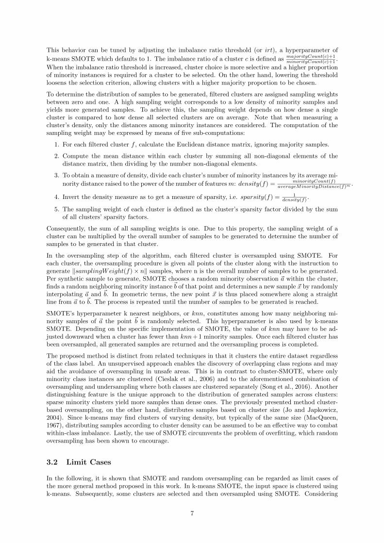
Input: X (matrix of observations)y (target vector)n (number of samples to be generated)k (number of clusters to be found by k-means)irt (imbalance ratio threshold)knn (number of nearest neighbors considered by SMOTE)de (exponent used for computation of density; defaults to the number of features in X)

begin// Step 1: Cluster the input space and filter clusters with more minority

instances than majority instances.

clusters← kmeans(X)filteredClusters← ∅for c ∈ clusters do

imbalanceRatio← majorityCount(c)+1minorityCount(c)+1

if imbalanceRatio < irt thenfilteredClusters← filteredClusters ∪ {c}

end

end

// Step 2: For each filtered cluster, compute the sampling weight based on its

minority density.

for f ∈ filteredClusters doaverageMinorityDistance(f)← mean(euclideanDistances(f))

densityFactor(f)← minorityCount(f)averageMinorityDistance(f)de

sparsityFactor(f)← 1densityFactor(f)

endsparsitySum←

∑f∈filteredClusters sparsityFactor(f)

samplingWeight(f)← sparsityFactor(f)sparsitySum

// Step 3: Oversample each filtered cluster using SMOTE. The number of samples to

be generated is computed using the sampling weight.

generatedSamples← ∅for f ∈ filteredClusters do

numberOfSamples← ‖n× samplingWeight(f)‖generatedSamples← generatedSamples ∪ {SMOTE(f, numberOfSamples, knn}

endreturn generatedSamples

endAlgorithm 1: Proposed method based on k-means and SMOTE

8

the case where the number of clusters k is equal to 1, all observations are grouped in one cluster. Forthis only cluster to be selected as a minority cluster, the imbalance ratio threshold needs to be setso that the imbalance ratio of the training data is met. For example, in a dataset with 100 minorityobservations and 10,000 majority observations, the imbalance ratio threshold must be greater than orequal to 10,000+1

100+1 ≈ 99.02. The single cluster is then selected and oversampled using SMOTE; sincethe cluster contains all observations, this is equivalent to simply oversampling the original dataset withSMOTE. Instead of setting the imbalance ratio threshold to the exact imbalance ratio of the dataset, itcan simply be set to positive infinity.

If SMOTE did not interpolate two different points to generate a new sample but performed the randominterpolation of one and the same point, the result would be a copy of the original point. This behaviorcould be achieved by setting the parameter “k nearest neighbors” of SMOTE to zero if the concreteimplementation supports this behavior. As such, random oversampling may be regarded as a specificcase of SMOTE.

This property of k-means SMOTE is of very practical value to its users: since it contains both SMOTEand random oversampling, a search of optimal hyperparameters could include the configurations for thosemethods. As a result, while a better parametrization may be found, the proposed method will performat least as well as the better of both oversamplers. In other words, SMOTE and random oversamplingare fallbacks contained in k-means SMOTE, which can be resorted to when the proposed method doesnot produce any gain with other parametrizations. Table 1 summarizes the parameters which may beused to reproduce the behavior of both algorithms.

k irt knn

SMOTE 1 ∞Random Oversampling 1 ∞ 0

Table 1: Limit case configurations

4 Research Methodology

The ultimate purpose of any resampling method is the improvement of classification results. In otherwords, a resampling technique is successful if the resampled data it produces improves the predictionquality of a given classifier. Therefore, the effectiveness of an oversampling method can only be assessedindirectly by evaluating a classifier trained on oversampled data. This proxy measure, i.e. the classifierperformance, is only meaningful when compared with the performance of the same classification algorithmtrained on data which has not been resampled. Multiple oversampling techniques can then be rankedby evaluating a classifier’s performance with respect to each modified training set produced by theresamplers.

A general concern in classifier evaluation is the bias of evaluating predictions for previously seen data.Classifiers may perform well when making predictions for rows of data used during training, but poorlywhen classifying new data. This problem is also referred to as overfitting. Oversampling techniques havebeen observed to encourage overfitting, which is why this bias should be carefully avoided during theirevaluation. A general approach is to split the available data into two or more subsets of which only oneis used during training, and another is used to evaluate the classification. The latter is referred to as theholdout set, unknown data, or test dataset.

Arbitrarily splitting the data into two sets, however, may introduce additional biases. One potentialissue that arises is that the resulting training set may not contain certain observations, preventing thealgorithm from learning important concepts. Cross-validation combats this issue by randomly splittingthe data many times, each time training the classifier from scratch using one portion of the data beforemeasuring its performance on the remaining share of data. After a number of repetitions, the classifier canbe evaluated by aggregating the results obtained in each iteration. In k-fold cross-validation, a popularvariant of cross-validation, k iterations, called folds, are performed. During each fold, the test set isone of k equally sized groups. Each group of observations is used exactly once as a holdout set. K-fold

9

cross-validation can be repeated many times to avoid potential bias due to random grouping (Japkowicz,2013).

While k-fold cross validation typically avoids the most important biases in classification tasks, it mightdistort the class distributions when randomly sampling from a class-imbalanced dataset. In the presenceof extreme skews, there may even be iterations where the test set contains no instances of the minorityclass, in which case classifier evaluation would be ill-defined or potentially strongly biased. A simpleand common approach to this problem is to use stratified cross-validation, where instead of samplingcompletely at random, the original class distribution is preserved in each fold (Japkowicz, 2013).

4.1 Metrics

Of the various assessment metrics traditionally used to evaluate classifier performance, not all are suitablewhen the class distribution is not uniform. However, there are metrics which have been employed ordeveloped specifically to cope with imbalanced data.

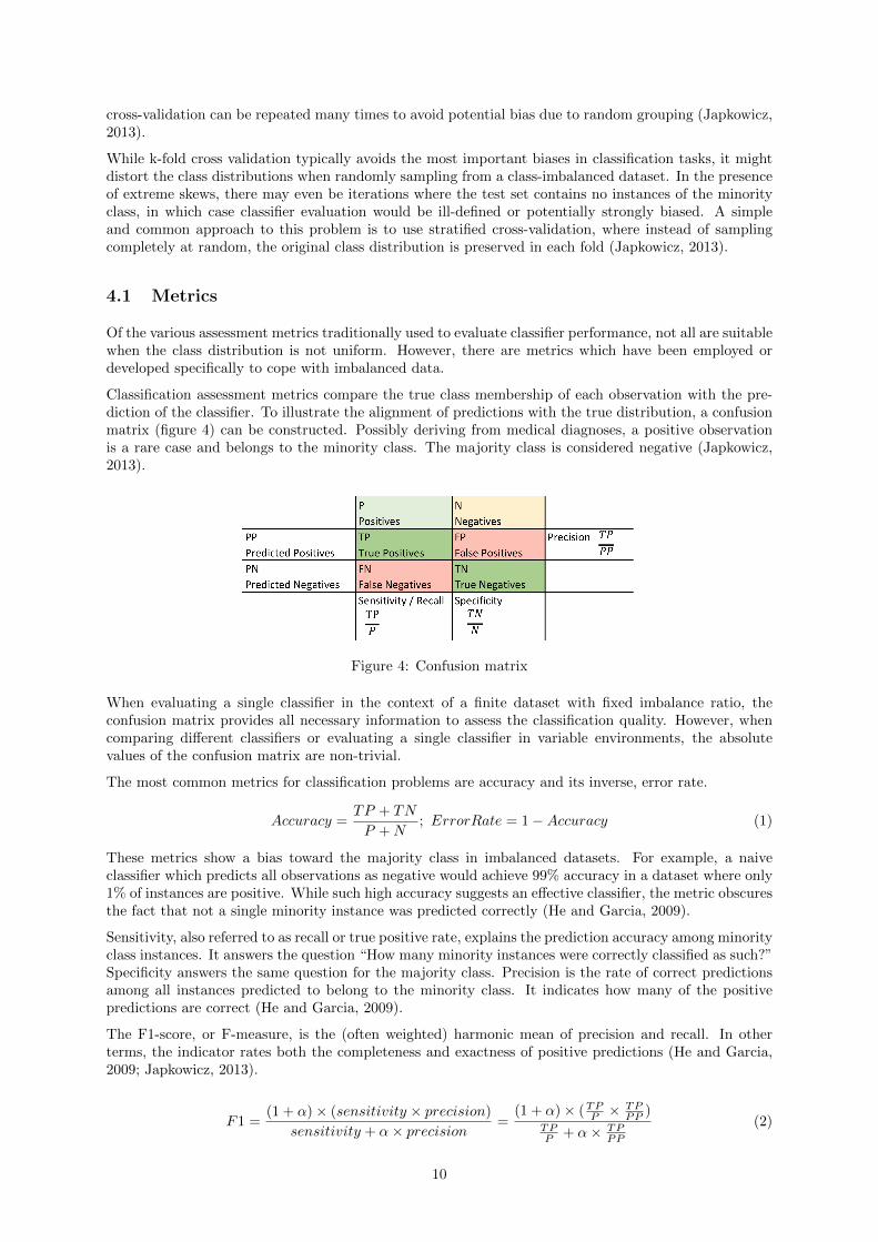
Classification assessment metrics compare the true class membership of each observation with the pre-diction of the classifier. To illustrate the alignment of predictions with the true distribution, a confusionmatrix (figure 4) can be constructed. Possibly deriving from medical diagnoses, a positive observationis a rare case and belongs to the minority class. The majority class is considered negative (Japkowicz,2013).

Figure 4: Confusion matrix

When evaluating a single classifier in the context of a finite dataset with fixed imbalance ratio, theconfusion matrix provides all necessary information to assess the classification quality. However, whencomparing different classifiers or evaluating a single classifier in variable environments, the absolutevalues of the confusion matrix are non-trivial.

The most common metrics for classification problems are accuracy and its inverse, error rate.

Accuracy =TP + TN

P +N; ErrorRate = 1−Accuracy (1)

These metrics show a bias toward the majority class in imbalanced datasets. For example, a naiveclassifier which predicts all observations as negative would achieve 99% accuracy in a dataset where only1% of instances are positive. While such high accuracy suggests an effective classifier, the metric obscuresthe fact that not a single minority instance was predicted correctly (He and Garcia, 2009).

Sensitivity, also referred to as recall or true positive rate, explains the prediction accuracy among minorityclass instances. It answers the question “How many minority instances were correctly classified as such?”Specificity answers the same question for the majority class. Precision is the rate of correct predictionsamong all instances predicted to belong to the minority class. It indicates how many of the positivepredictions are correct (He and Garcia, 2009).

The F1-score, or F-measure, is the (often weighted) harmonic mean of precision and recall. In otherterms, the indicator rates both the completeness and exactness of positive predictions (He and Garcia,2009; Japkowicz, 2013).

F1 =(1 + α)× (sensitivity × precision)

sensitivity + α× precision=

(1 + α)× (TPP ×

TPPP )

TPP + α× TP

PP

(2)

10

The geometric mean score, also referred to as g-mean or g-measure, is defined as the geometric mean ofsensitivity and specificity. The two components can be regarded as per-class accuracy. The g-measureaggregates both metrics into a single value in [0, 1], assigning equal importance to both (He and Garcia,2009; Japkowicz, 2013).

g-mean =√sensitivity × specificity =

√TP

P× TN

N(3)

Precision-recall (PR) diagrams plot the precision of a classifier as a function of its minority accuracy.Classifiers outputting class membership confidences (i.e. continuous values in [0, 1]) can be plotted as mul-tiple points in discrete intervals, resulting in a PR curve. Commonly, the area under the precision-recallcurve (AUPRC) is computed as a single numeric performance metric (He and Garcia, 2009; Japkowicz,2013).

The choice of metric depends to a great extent on the goal their user seeks to achieve. In certain practicaltasks, one specific aspect of classification may be more important than another (e.g. in medical diagnoses,false negatives are much more critical than false positives). However, to determine a general rankingamong oversamplers, no such focus should be placed. Therefore, the following unweighted metrics arechosen for the evaluation.

• g-mean

• F1-score

• AUPRC

4.2 Oversamplers

The following list enumerates the oversamplers used as a benchmark for the evaluation of the proposedmethod, along with the set of hyperparameters used for each. The optimal imbalance ratio is not obviousand has been discussed by other researchers (Provost, 2000; Estabrooks et al., 2004). This work aims atcreating comparability among oversamplers; consequently, it is most important that oversamplers achievethe same imbalance ratio. Therefore, all oversampling methods were parametrized to generate as manyinstances as necessary so that minority and majority classes count the same number of samples.

• random oversampling

• SMOTE

– knn ∈ {3, 5, 20}

• borderline-SMOTE1

– knn ∈ {3, 5, 20}

• borderline-SMOTE2

– knn ∈ {3, 5, 20}

• k-means SMOTE

– k ∈ {2, 20, 50, 100, 250, 500}

– knn ∈ {3, 5, 20,∞}

– irt ∈ {1,∞}

– de ∈ {0, 2, numberOfFeatures}

• no oversampling

11

4.3 Classifiers

For the evaluation of the various oversampling methods, several different classifiers are chosen to ensurethat the results obtained can be generalized and are not constrained to the usage of a specific classifier.The choice of classifiers is further motivated by the number of hyperparameters: classification algorithmswith few or no hyperparameters are less likely to bias results due to their specific configuration.

Logistic regression (LR) is a generalization of linear regression which can be used for binary classification.Fitting the model is an optimization problem which can be solved using simple optimizers which requireno hyperparameters to be set (McCullagh, 1984). Consequently, results achieved by LR are easilyreproducible, while also constituting a baseline for more sophisticated approaches.

Another classification algorithm referred to as k-nearest neighbors (KNN) assigns an observation to theclass most of its nearest neighbors belong to. How many neighbors are considered is determined by themethod’s hyperparameter k (Fix and Hodges Jr., 1951).

Finally, gradient boosting over decision trees, or simply gradient boosting machine (GBM), is an ensembletechnique used for classification. In the case of binary classification, one shallow decision tree is inducedat each stage of the algorithm. Each tree is fitted to observations which could not be correctly classifiedby decision trees of previous stages. Predictions of GBM are made by majority vote of all trees. In thisway, the algorithm combines several simple models (referred to as weak learners) to create one effectiveclassifier. The number of decision trees to generate, which in binary classification is equal to the numberof stages, is a hyperparameter of the algorithm (Friedman, 2001).

As further explained in section 4.5, various combinations of hyperparameters are tested for each classifier.All classifiers are used as implemented in the python library scikit-learn (Pedregosa et al., 2011) withdefault parameters unless stated otherwise. The following list enumerates the classifiers used in thisstudy along with a set of values for their respective hyperparameters.

• LR

• KNN

– k ∈ {3, 5, 8}

• GBM

– numberOfTrees ∈ {50, 100, 200}

4.4 Datasets

To evaluate k-means SMOTE, 12 imbalanced datasets from the UCI Machine Learning Repository (Lich-man, 2013) are used. Those datasets containing more than two classes were binarized using a one-versus-rest approach, labeling the smallest class as the minority and merging all other samples into one class.In order to generate additional datasets with even higher imbalance ratios, each of the aforementioneddatasets was randomly undersampled to generate up to six additional datasets. The imbalance ratio ofeach dataset was increased approximately by multiplication factors of 2, 4, 6, 10, 15 and 20, but only if agiven factor did not reduce a dataset’s total number of minority samples to less than eight. Furthermore,the python library scikit-learn (Pedregosa et al., 2011) was used to generate ten variations of the artificial“MADELON” dataset, which poses a difficult binary classification problem (Guyon, 2003).

Table 2 lists the datasets used to evaluate the proposed method, along with important characteristics.The artificial datasets are referred to as simulated. Undersampled versions of the original datasetsare omitted from the table. All datasets used in the study are made available at https://github.com/felix-last/evaluate-kmeans-smote/releases/download/v0.0.1/uci_extended.tar.gz for the pur-pose of reproducibility.

4.5 Experimental Framework

To evaluate the proposed method, the oversamplers, metrics, datasets, and classifiers discussed in thissection are used. Results are obtained by repeating 5-fold cross-validation five times. For each dataset,

12

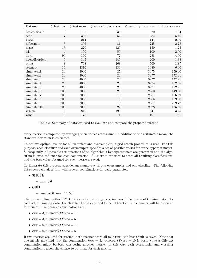
Dataset # features # instances # minority instances # majority instances imbalance ratio

breast tissue 9 106 36 70 1.94ecoli 7 336 52 284 5.46glass 9 214 70 144 2.06haberman 3 306 81 225 2.78heart 13 270 120 150 1.25iris 4 150 50 100 2.00libra 90 360 72 288 4.00liver disorders 6 345 145 200 1.38pima 8 768 268 500 1.87segment 16 2310 330 1980 6.00simulated1 20 4000 25 3975 159.00simulated2 20 4000 23 3977 172.91simulated3 20 4000 23 3977 172.91simulated4 20 4000 26 3974 152.85simulated5 20 4000 23 3977 172.91simulated6 200 3000 20 2980 149.00simulated7 200 3000 19 2981 156.89simulated8 200 3000 15 2985 199.00simulated9 200 3000 13 2987 229.77simulated10 200 3000 22 2978 135.36vehicle 18 846 199 647 3.25wine 13 178 71 107 1.51

Table 2: Summary of datasets used to evaluate and compare the proposed method

every metric is computed by averaging their values across runs. In addition to the arithmetic mean, thestandard deviation is calculated.

To achieve optimal results for all classifiers and oversamplers, a grid search procedure is used. For thispurpose, each classifier and each oversampler specifies a set of possible values for every hyperparameter.Subsequently, all possible combinations of an algorithm’s hyperparameters are generated and the algo-rithm is executed once for each combination. All metrics are used to score all resulting classifications,and the best value obtained for each metric is saved.

To illustrate this process, consider an example with one oversampler and one classifier. The followinglist shows each algorithm with several combinations for each parameter.

• SMOTE

– knn: 3,6

• GBM

– numberOfTrees: 10, 50

The oversampling method SMOTE is run two times, generating two different sets of training data. Foreach set of training data, the classifier LR is executed twice. Therefore, the classifier will be executedfour times. The possible combinations are:

• knn = 3, numberOfTrees = 10

• knn = 3, numberOfTrees = 50

• knn = 6, numberOfTrees = 10

• knn = 6, numberOfTrees = 50

If two metrics are used for scoring, both metrics score all four runs; the best result is saved. Note thatone metric may find that the combination knn = 3, numberOfTrees = 10 is best, while a differentcombination might be best considering another metric. In this way, each oversampler and classifiercombination is given the chance to optimize for each metric.

13

5 Experimental Results

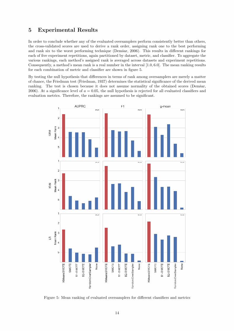
In order to conclude whether any of the evaluated oversamplers perform consistently better than others,the cross-validated scores are used to derive a rank order, assigning rank one to the best performingand rank six to the worst performing technique (Demsar, 2006). This results in different rankings foreach of five experiment repetitions, again partitioned by dataset, metric, and classifier. To aggregate thevarious rankings, each method’s assigned rank is averaged across datasets and experiment repetitions.Consequently, a method’s mean rank is a real number in the interval [1.0, 6.0]. The mean ranking resultsfor each combination of metric and classifier are shown in figure 5.

By testing the null hypothesis that differences in terms of rank among oversamplers are merely a matterof chance, the Friedman test (Friedman, 1937) determines the statistical significance of the derived meanranking. The test is chosen because it does not assume normality of the obtained scores (Demsar,2006). At a significance level of a = 0.05, the null hypothesis is rejected for all evaluated classifiers andevaluation metrics. Therefore, the rankings are assumed to be significant.

Figure 5: Mean ranking of evaluated oversamplers for different classifiers and metrics

14

The mean ranking shows that the proposed method outperforms other methods with regard to allevaluation metrics. Notably, the technique’s superiority can be observed independently of the classifier.In six out of nine cases, k-means SMOTE achieves a mean rank better than two, whereas in the otherthree cases the mean rank is at least three. Furthermore, k-means SMOTE is the only technique with amean ranking better than three with respect to F1 score and AUPRC. This observation suggests thatk-means SMOTE improves classification results even when other oversamplers accomplish a similar rankas classifying without oversampling.

Generally, it can be observed that - aside from the proposed method - SMOTE, borderline-SMOTE1, andborderline-SMOTE2 typically achieve the best results, while not oversampling usually earns the worstrank. Remarkably, LR achieves a similar rank without oversampling as with SMOTE with regard toAUPRC, while both are only dominated by k-means SMOTE. This indicates that the proposed methodmay improve classification results even when SMOTE is not able to achieve any improvement versus theoriginal training data.

For a direct comparison to the baseline method, SMOTE, the average optimal scores attained by k-meansSMOTE for each dataset are subtracted by the respective scores reached by SMOTE. The resulting scoreimprovements achieved by the proposed method are summarized in figures 6 and 7.

Figure 6: Mean score improvement of the proposedmethod versus SMOTE across datasets

Figure 7: Maximum score improvement of the pro-posed method versus SMOTE

The KNN classifier appears to profit most from the application of k-means SMOTE, where maximumscore improvements of more than 0.2 are observed across all metrics. The biggest mean score improve-ments are also achieved using KNN, with a 0.034 average improvement with regard to the AUPRCmetric. It can further be observed that all classifiers benefit from the application of k-means SMOTE.With one exception, maximum score improvements of more than 0.1 are achieved for all classifiers andmetrics.

Taking a closer look at the combination of classifier and metric which, on average, benefit most fromthe application of the proposed method, figure 8 shows the AUPRC achieved by the two methods inconjunction with the KNN classifier for each dataset. Although absolute scores and score differencesbetween the two methods are dependent on the choice of metric and classifier, the general trend shownin the figure is observed for all other metrics and classifiers, which are omitted for clarity.

In the large majority of cases, k-means SMOTE outperforms SMOTE, proving the relevance of theclustering procedure. Only in 2 out of 71 datasets tested there were no improvements through the use ofk-means SMOTE. On average, k-means SMOTE achieves an AUPRC improvement of 0.034. The biggestgains of the proposed method appear to be occurring in the score range of 0.2 to 0.8. On the lower endof that range, k-means SMOTE achieves an average gain of more than 0.2 compared to SMOTE in the“glass6” dataset. Prediction of dataset “vehicle15” is improved from an AUPRC of approximately 0.35to 0.5. The third biggest gain occurs in the “ecoli6” dataset, where the proposed method obtains a scoreof 0.8 compared to less than 0.7 accomplished by SMOTE. The score difference among oversamplersis smaller at the extreme ends of the scale. For nine of the simulated datasets, KNN attains a scorevery close to zero independently of the choice of the oversampler. Similarly, for the datasets where anAUPRC around 0.95 is attained (“libra”, “libra2”, “iris”, “iris6”), gains of k-means SMOTE are lessthan 0.02.

15

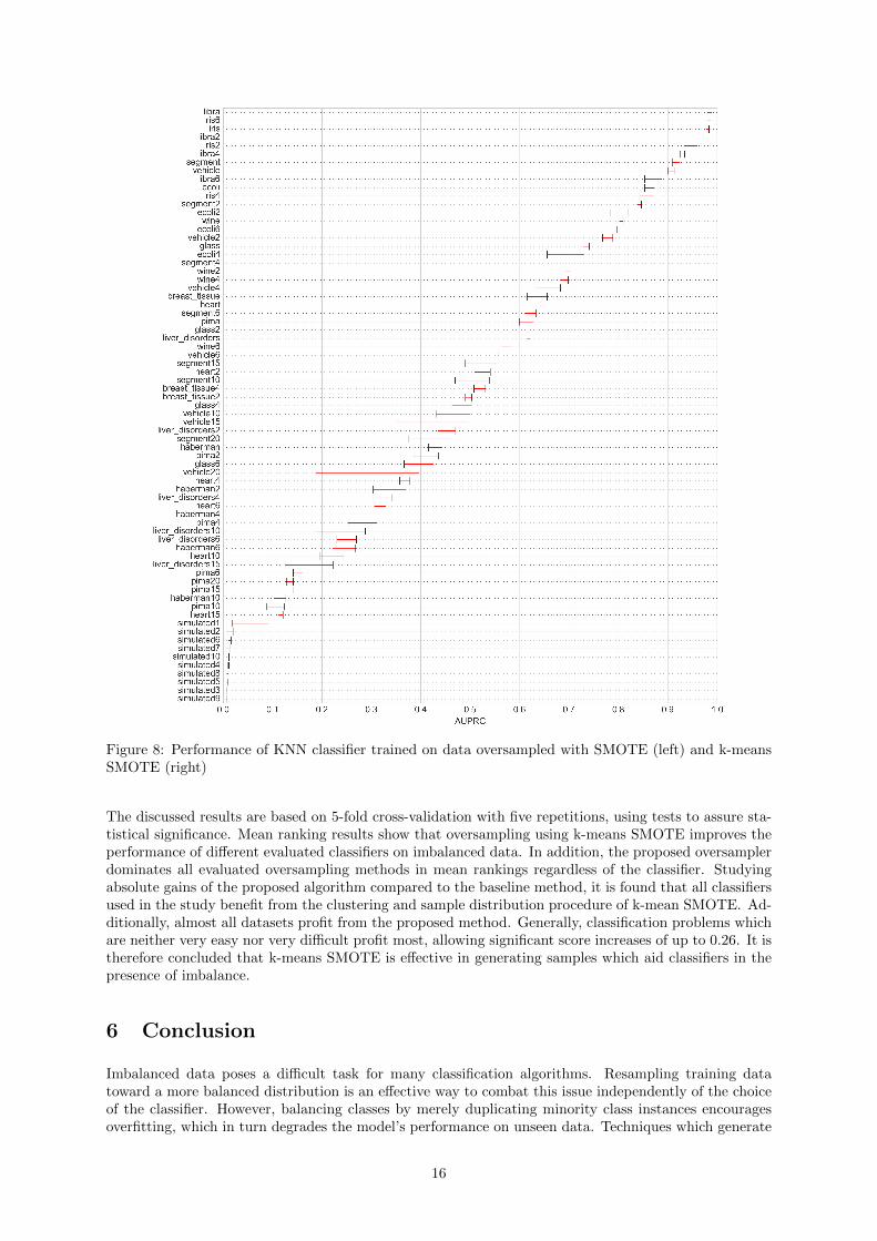
Figure 8: Performance of KNN classifier trained on data oversampled with SMOTE (left) and k-meansSMOTE (right)

The discussed results are based on 5-fold cross-validation with five repetitions, using tests to assure sta-tistical significance. Mean ranking results show that oversampling using k-means SMOTE improves theperformance of different evaluated classifiers on imbalanced data. In addition, the proposed oversamplerdominates all evaluated oversampling methods in mean rankings regardless of the classifier. Studyingabsolute gains of the proposed algorithm compared to the baseline method, it is found that all classifiersused in the study benefit from the clustering and sample distribution procedure of k-mean SMOTE. Ad-ditionally, almost all datasets profit from the proposed method. Generally, classification problems whichare neither very easy nor very difficult profit most, allowing significant score increases of up to 0.26. It istherefore concluded that k-means SMOTE is effective in generating samples which aid classifiers in thepresence of imbalance.

6 Conclusion

Imbalanced data poses a difficult task for many classification algorithms. Resampling training datatoward a more balanced distribution is an effective way to combat this issue independently of the choiceof the classifier. However, balancing classes by merely duplicating minority class instances encouragesoverfitting, which in turn degrades the model’s performance on unseen data. Techniques which generate

16

artificial samples, on the other hand, often suffer from a tendency to generate noisy samples, impedingthe inference of class boundaries. Moreover, most existing oversamplers do not counteract imbalanceswithin the minority class, which is often a major issue when classifying class-imbalanced datasets. Foroversampling to effectively aid classifiers, the amplification of noise should be avoided by detecting safeareas of the input space where class regions do not overlap. Additionally, any imbalance within theminority class should be identified and samples are to be generated as to level the distribution.

The proposed method achieves these properties by clustering the data using k-means, allowing to focusdata generation on crucial areas of the input space. A high ratio of minority observations is used asan indicator that a cluster is a safe area. Oversampling only safe clusters enables k-means SMOTE toavoid noise generation. Furthermore, the average distance among a cluster’s minority samples is usedto discover sparse areas. Sparse minority clusters are assigned more synthetic samples, which alleviateswithin-class imbalance. Finally, overfitting is discouraged by generating genuinely new observations usingSMOTE rather than replicating existing ones.

Empirical results show that training various types of classifiers using data oversampled with k-meansSMOTE leads to better classification results than training with unmodified, imbalanced data. Moreimportantly, the proposed method consistently outperforms the most widely available oversampling tech-niques such as SMOTE, borderline-SMOTE, and random oversampling. The biggest gains appear tobe achieved in classification problems which are neither extremely difficult nor extremely simple. Theresults are statistically robust and apply to various metrics suited for the evaluation of imbalanced dataclassification.

The effectiveness of the algorithm is accomplished without high complexity. The method’s components,k-means clustering and SMOTE oversampling, are simple and readily available in many programminglanguages, so that practitioners and researchers may easily implement and use the proposed method intheir preferred environment. Further facilitating practical use, an implementation of k-means SMOTEin the python programming language is made available (see https://github.com/felix-last/kmeans_smote) based on the imbalanced-learn framework (Lemaıtre et al., 2017).

A prevalent issue in classification tasks, data imbalance is exhibited naturally in many important real-world applications. As the proposed oversampler can be applied to rebalance any dataset and inde-pendently of the chosen classifier, its potential impact is substantial. Among others, k-means SMOTEmay, therefore, contribute to the prevention of credit card fraud, the diagnosis of diseases, as well as thedetection of abnormalities in environmental observations.

Future work may consequently focus on applying k-means SMOTE to various other real-world problems.Additionally, finding optimal values of k and other hyperparameters is yet to be guided by rules of thumb,which could be deducted from further analyses of the relationship between optimal hyperparameters fora given dataset and the dataset’s properties.

References

Batista, G. E. A. P. A., Prati, R. C., and Monard, M. C. (2004). A study of the behavior of sev-eral methods for balancing machine learning training data. ACM SIGKDD Explorations Newsletter,6(1):20–29.

Bunkhumpornpat, C., Sinapiromsaran, K., and Lursinsap, C. (2009). Safe-level-smote: Safe-level-synthetic minority over-sampling technique for handling the class imbalanced problem. In LectureNotes in Computer Science (including subseries Lecture Notes in Artificial Intelligence and LectureNotes in Bioinformatics), volume 5476 LNAI, pages 475–482.

Chawla, N. V., Bowyer, K. W., Hall, L. O., and Kegelmeyer, W. P. (2002). Smote: Synthetic minorityover-sampling technique. Journal of Artificial Intelligence Research, 16:321–357.

Chawla, N. V., Japkowicz, N., and Drive, P. (2004). Editorial: Special issue on learning from imbalanceddata sets. ACM SIGKDD Explorations Newsletter, 6(1):1–6.

Cieslak, D. A., Chawla, N. V., and Striegel, A. (2006). Combating imbalance in network intrusiondatasets. In Granular Computing, 2006 IEEE International Conference on, pages 732–737. IEEE.

17

Demsar, J. (2006). Statistical comparisons of classifiers over multiple data sets. Journal of Machinelearning research, 7(Jan):1–30.

Domingos, P. (1999). Metacost: A general method for making classifiers. In Proceedings of the 5thInternational Conference on Knowledge Discovery and Data Mining, pages 155–164.

Douzas, G. and Bacao, F. (2017). Self-organizing map oversampling (somo) for imbalanced data setlearning. Expert Systems with Applications, 82:40–52.

Estabrooks, A., Jo, T., and Japkowicz, N. (2004). A multiple resampling method for learning fromimbalanced data sets. Computational intelligence, 20(1):18–36.

Fernandez, A., Lopez, V., Galar, M., Del Jesus, M. J., and Herrera, F. (2013). Analysing the classifi-cation of imbalanced data-sets with multiple classes: Binarization techniques and ad-hoc approaches.Knowledge-Based Systems, 42:97–110.

Fix, E. and Hodges Jr., J. (1951). Discriminatory analysis - nonparametric discrimination: Consistencyproperties.

Friedman, J. H. (2001). Greedy function approximation: A gradient boosting machine. Annals ofStatistics, 29(5):1189–1232.

Friedman, M. (1937). The use of ranks to avoid the assumption of normality implicit in the analysis ofvariance. Journal of the American Statistical Association, 32(200):675.

Galar, M., Fernandez, A., Barrenechea, E., Bustince, H., and Herrera, F. (2012). A review on ensemblesfor the class imbalance problem: Bagging-, boosting-, and hybrid-based approaches.

Guyon, I. (2003). Design of experiments of the nips 2003 variable selection benchmark.

Han, H., Wang, W.-Y., and Mao, B.-H. (2005). Borderline-smote: A new over-sampling method inimbalanced data sets learning. Advances in intelligent computing, 17(12):878–887.

Hawkins, D. M. (2004). The problem of overfitting. Journal of chemical information and computersciences, 44(1):1–12.

He, H. and Garcia, E. A. (2009). Learning from imbalanced data. IEEE Transactions on Knowledge andData Engineering, 21(9):1263–1284.

Holte, R. C., Acker, L., Porter, B. W., et al. (1989). Concept learning and the problem of small disjuncts.In IJCAI, volume 89, pages 813–818.

Japkowicz, N. (2013). Assessment metrics for imbalanced learning. In He, H. and Ma, Y., editors,Imbalanced learning, pages 187–206. John Wiley & Sons.

Jo, T. and Japkowicz, N. (2004). Class imbalances versus small disjuncts. ACM SIGKDD ExplorationsNewsletter, 6(1):40–49.

Kotsiantis, S., Kanellopoulos, D., and Pintelas, P. (2006). Handling imbalanced datasets: A review.Science, 30(1):25–36.

Kotsiantis, S., Pintelas, P., Anyfantis, D., and Karagiannopoulos, M. (2007). Robustness of learningtechniques in handling class noise in imbalanced datasets.

Lemaıtre, G., Nogueira, F., and Aridas, C. K. (2017). Imbalanced-learn: A Python Toolbox to Tackle theCurse of Imbalanced Datasets in Machine Learning. Journal of Machine Learning Research, 18(17):1–5.

Lichman, M. (2013). Uci machine learning repository.

Ma, L. and Fan, S. (2017). Cure-smote algorithm and hybrid algorithm for feature selection and param-eter optimization based on random forests. BMC bioinformatics, 18(1):169.

MacQueen, J. (1967). Some methods for classification and analysis of multivariate observations. InProceedings of the fifth Berkeley symposium on mathematical statistics and probability, volume 1, pages281–297.

18

McCullagh, P. (1984). Generalized linear models. European Journal of Operational Research, 16(3):285–292.

Nekooeimehr, I. and Lai-Yuen, S. K. (2016). Adaptive semi-unsupervised weighted oversampling (a-suwo)for imbalanced datasets. Expert Systems with Applications, 46:405–416.

Nickerson, A., Japkowicz, N., and Milios, E. E. (2001). Using unsupervised learning to guide resamplingin imbalanced data sets. In AISTATS.

Pedregosa, F., Varoquaux, G., Gramfort, A., Michel, V., Thirion, B., Grisel, O., Blondel, M., Pretten-hofer, P., Weiss, R., Dubourg, V., Vanderplas, J., Passos, A., Cournapeau, D., Brucher, M., Perrot,M., and Duchesnay, E. (2011). Scikit-learn: Machine learning in python. Journal of Machine learningresearch, 12:2825–2830.

Prati, R. C., Batista, G., and Monard, M. C. (2004). Learning with class skews and small disjuncts. InSBIA, pages 296–306.

Provost, F. (2000). Machine learning from imbalanced data sets 101. In Proceedings of the AAAI’2000workshop on imbalanced data sets, volume 68, pages 1–3. AAAI Press.

Santos, M. S., Abreu, P. H., Garcıa-Laencina, P. J., Simao, A., and Carvalho, A. (2015). A new cluster-based oversampling method for improving survival prediction of hepatocellular carcinoma patients.Journal of biomedical informatics, 58:49–59.

Sculley, D. (2010). Web-scale k-means clustering. In Proceedings of the 19th international conference onWorld wide web, pages 1177–1178, 1772690. ACM.

Song, J., Huang, X., Qin, S., and Song, Q. (2016). A bi-directional sampling based on k-means methodfor imbalance text classification. In Computer and Information Science (ICIS), 2016 IEEE/ACIS 15thInternational Conference on, pages 1–5.

Weiss, G. M., McCarthy, K., and Zabar, B. (2007). Cost-sensitive learning vs. sampling: Which is bestfor handling unbalanced classes with unequal error costs? DMIN, 7:35–41.

19