ov real-time systems gilad koren - cs.nyu.edu · comp etitiv e on-line sc heduling for ov erloaded...
TRANSCRIPT
Competitive On-Line Scheduling
for
Overloaded Real-Time Systems
by
Gilad Koren
a dissertation submitted in partial fulfillment
of the requirements for the degree of
Doctor of Philosophy
Department of Computer Science
New York University
September 1993
Approved
Dennis Shasha
Advisor
Bhubaneswar Mishra
Co-Advisor
c Gilad Koren
All Rights Reserved, 1993.


Dedication
I would like to dedicate this work to the memory of my beloved uncle Ignatz Brand who
passed away while this work was in progress.
v
Acknowledgments
This work was made possible by a big investment on the part of my advisor Dennis Shasha
both in time and talent. Dennis was constantly pushing forward, raising new questions
and suggesting new ideas. I owe him a lot for showing me the way through graduate school
(including crossing the Atlantic to Paris and back). Karen and Dennis Shasha became
part of my extended family. I enjoyed their international Thursday night dinners in Paris
(where I played the dish washer role) and many other occasions where we spent time
together.
I would like to thank my co-advisor Bud Mishra for his guidance and encouragement.
Bud spent many hours with me, always contributing a new and clear perspective of the
problems and the solutions. It was Marc Donner that introduced my advisors to the �eld
of Real Time Scheduling in a seminar he gave in NYU (which I regret deeply for having
overlooked at that time). Marc has been very supportive throughout this work, willing to
listen and to give advice always with a smile. Some of this work was done while visiting in
INRIA, Rocouncourt, France. I would like to thank Patrick Valduriez and all the people
of Project Rodin for their hospitality.
My aunt and uncle Frega and Ignatz Brand helped me in all possible ways through out
my New York experience, always willing to listen and to support. I should not forget my
good friends who had a big stake in my life during graduate school: Gadi, Eddie, Arnon,
Andres and last but not the least Jenifer (with one `n'). Vekamuvan hamishpahca ba'aretz
she'azra li harbe: Ima, Neomi, Srulik, Shachar and Tali.
The illustration is by Marianna Tro�mova.
Work on this dissertation was supported by U.S. O�ce of Naval Research grants #N00014-
91-J-1472 and #N00014-92-J-1719, U.S. National Science Foundation grant #CCR-9103953.
vi
Abstract
We study competitive on-line scheduling in uniprocessor and multiprocessor real-time en-
vironments. In our model, tasks are sporadic and preemptible. Every task has a deadline
and a value that the system obtains only if the task completes its execution by its dead-
line. The aim of a scheduler is to maximize the total value obtained from all the tasks that
complete before their deadline.
An on-line scheduler has no knowledge of a task until it is released. The problem is to
design an on-line scheduler with worst case guarantees even in the presence of overloaded
periods. The guarantee is given in terms of a positive competitive factor. We say that
an on-line algorithm has a competitive factor of r, 0 < r � 1, when under all possible
circumstances (i.e, task sets) the scheduler will get at least r times the best possible value.
The best value is the value obtained by a clairvoyant algorithm. In contrast to an on-line
scheduler, the clairvoyant algorithm knows the entire task set a priori at time zero.
When a uniprocessor system is underloaded there exist several optimal on-line algo-
rithms that will schedule all tasks to completion (e.g., the Earliest Deadline First algo-
rithm). However, under overload, these algorithms perform poorly. Heuristics have been
proposed to deal with overloaded situations but these give no worst case guarantees.
We present an optimal on-line scheduling algorithm for uniprocessor overloaded systems
called D-over. D-over is optimal in the sense that it has the best competitive factor possible.
Moreover, while the system is underloaded, D-over will obtain 100% of the possible value.
In the multiprocessor case, we study systems with two or more processors. We present
an inherent limit (lower bound) on the best competitive guarantee that any on-line parallel
real-time scheduler can give. Then we present a competitive algorithm that achieves a worst
case guarantee which is within a small factor from the best possible guarantee in many
cases.
vii
Contents
Dedication v
Acknowledgments vi
Abstract vii
List of Figures xi
List of Tables xii
1 Introduction 1
1.1 Introduction : : : : : : : : : : : : : : : : : : : : : : : : : : : : : : : : : : : : 2
1.1.1 Real-Time Systems : : : : : : : : : : : : : : : : : : : : : : : : : : : : 2
1.1.2 Scheduling : : : : : : : : : : : : : : : : : : : : : : : : : : : : : : : : 2
1.2 Background : : : : : : : : : : : : : : : : : : : : : : : : : : : : : : : : : : : : 4
1.2.1 Optimal Scheduling Algorithms : : : : : : : : : : : : : : : : : : : : : 7
1.2.2 Rate Monotonic Scheduling : : : : : : : : : : : : : : : : : : : : : : : 7
1.2.3 Time-driven Optimal Schedulers : : : : : : : : : : : : : : : : : : : : 8
1.2.4 Multiprocessor Optimal Scheduling : : : : : : : : : : : : : : : : : : : 9
1.3 Scheduling in the Presence of Overload : : : : : : : : : : : : : : : : : : : : : 10
1.4 Our Model of Real-Time System : : : : : : : : : : : : : : : : : : : : : : : : 11
1.4.1 Competitive On-Line Schedulers : : : : : : : : : : : : : : : : : : : : 12
1.5 Main Results : : : : : : : : : : : : : : : : : : : : : : : : : : : : : : : : : : : 14
1.5.1 Uniprocessor Environments : : : : : : : : : : : : : : : : : : : : : : : 14
1.5.2 Multiprocessor Environments : : : : : : : : : : : : : : : : : : : : : : 15
viii
1.6 Dissertation Overview : : : : : : : : : : : : : : : : : : : : : : : : : : : : : : 16
2 Notation and Assumptions 17
3 Uniprocessor Environments 20
3.1 Dover: : : : : : : : : : : : : : : : : : : : : : : : : : : : : : : : : : : : : : : : 21
3.2 Analysis of Dover: : : : : : : : : : : : : : : : : : : : : : : : : : : : : : : : : 26
3.2.1 Proof Strategy : : : : : : : : : : : : : : : : : : : : : : : : : : : : : : 30
3.2.2 Some Lemmas about Dover's Scheduling : : : : : : : : : : : : : : : : 31
3.2.3 How Well Can a Clairvoyant Scheduler Do? : : : : : : : : : : : : : : 36
3.2.4 The Running Complexity of Dover: : : : : : : : : : : : : : : : : : : 44
3.3 Underloaded Periods: Con icting Tasks : : : : : : : : : : : : : : : : : : : : 45
4 Multiprocessor Environments 48
4.1 The Lower Bound : : : : : : : : : : : : : : : : : : : : : : : : : : : : : : : : 49
4.2 Algorithmic Guarantees : : : : : : : : : : : : : : : : : : : : : : : : : : : : : 56
4.3 The Algorithm's Competitive Multiplier : : : : : : : : : : : : : : : : : : : : 62
4.3.1 Setting : : : : : : : : : : : : : : : : : : : : : : : : : : : : : : : : : 67
4.3.2 Distributed vs. Centralized Scheduler : : : : : : : : : : : : : : : : : 68
4.3.3 The Scheduling Overhead : : : : : : : : : : : : : : : : : : : : : : : : 70
5 Conclusions 71
Bibliography 77
A Underloaded Periods: Con icting Tasks 81
A.1 The Remove Con ict Procedure : : : : : : : : : : : : : : : : : : : : : : : : : 82
A.1.1 The Performance Guarantee of Dover : : : : : : : : : : : : : : : : : : 84
B Dover: Gradual Descent 89
B.1 Exponential Gradual Descent : : : : : : : : : : : : : : : : : : : : : : : : : : 90
B.2 A Variant of Dover for Gradual Descent : : : : : : : : : : : : : : : : : : : : 90
B.3 Analysis of Dover in the Gradual Descent Model : : : : : : : : : : : : : : : : 91
B.3.1 Lemmas about Dover 's Scheduling : : : : : : : : : : : : : : : : : : : 91
B.3.2 How Well Can a Clairvoyant Scheduler Do? : : : : : : : : : : : : : : 92
ix
B.4 Inherent Bounds : : : : : : : : : : : : : : : : : : : : : : : : : : : : : : : : : 97
B.5 Performance Guarantee for Underloaded Periods : : : : : : : : : : : : : : : 97
B.6 Other Gradual Descent Schemes : : : : : : : : : : : : : : : : : : : : : : : : 97
C Dover: Exact Computation Time Is Not Known 99
C.1 An Inherent Bound On The Competitive Multiplier : : : : : : : : : : : : : : 101
C.2 Underloaded Systems : : : : : : : : : : : : : : : : : : : : : : : : : : : : : : : 101
C.3 Overloaded Systems : : : : : : : : : : : : : : : : : : : : : : : : : : : : : : : 102
D Two Processor Systems 105
D.1 The Safe-Risky Algorithm : : : : : : : : : : : : : : : : : : : : : : : : : : : : 106
D.2 The Competitive Multiplier of the Safe-Risky algorithm : : : : : : : : : : : 109
D.3 When Task Migration is Not Allowed : : : : : : : : : : : : : : : : : : : : : : 116
D.3.1 The Safe-Risky-(�xed) Algorithm : : : : : : : : : : : : : : : : : : : : 116
D.3.2 Analysis : : : : : : : : : : : : : : : : : : : : : : : : : : : : : : : : : : 117
D.4 Scheduling Overhead : : : : : : : : : : : : : : : : : : : : : : : : : : : : : : : 117
x
List of Figures
2.1 D The Earliest Deadline First scheduling algorithm. : : : : : : : : : : : : : 18
3.1 Dover- A Competitive optimal on-line scheduling algorithm. : : : : : : : : : 23
3.2 Dover (cont.) : : : : : : : : : : : : : : : : : : : : : : : : : : : : : : : : : : : 24
3.3 Dover (cont.) : : : : : : : : : : : : : : : : : : : : : : : : : : : : : : : : : : : 25
3.4 Dover (cont.) : : : : : : : : : : : : : : : : : : : : : : : : : : : : : : : : : : : 26
3.5 The Remove Con icts algorithm. : : : : : : : : : : : : : : : : : : : : : : : : 46
4.1 A complete set for n = 3 and k = 8. : : : : : : : : : : : : : : : : : : : : : : 50
4.2 A schematic description of the MOCA Algorithm. : : : : : : : : : : : : : : : 59
4.3 The MOCA Algorithm scheduling for example 4.2.1. : : : : : : : : : : : : : 61
4.4 The ratio between the value guaranteed to be obtained by the algorithm
and the lower bound for varying number of processors and importance ratios. 69
5.1 Comparison of of lower bounds and algorithmic bounds for varying number
of processors. : : : : : : : : : : : : : : : : : : : : : : : : : : : : : : : : : : 74
D.1 The Safe-Risky algorithm- a scheduler for two processors systems. : : : : : 107
D.2 The Safe-Risky algorithm- the Latest Start Time and the Task Completion
routines. : : : : : : : : : : : : : : : : : : : : : : : : : : : : : : : : : : : : : : 108
D.3 The Safe-Risky-(�xed) algorithm. : : : : : : : : : : : : : : : : : : : : : : : 116
xi
List of Tables
3.1 The tasks for example 3.2.2. : : : : : : : : : : : : : : : : : : : : : : : : : : : 29
3.2 Dover's scheduling for example 3.2.2. : : : : : : : : : : : : : : : : : : : : : : 31
4.1 The tasks for example 4.2.1. : : : : : : : : : : : : : : : : : : : : : : : : : : : 60
5.1 State of the art of competitive real time scheduling. : : : : : : : : : : : : : 72
A.1 Tasks for example A.1.1. : : : : : : : : : : : : : : : : : : : : : : : : : : : : : 83
A.2 Aggregated tasks for example A.1.1. : : : : : : : : : : : : : : : : : : : : : : 83
xii
Chapter 1
Introduction
1
CHAPTER 1. INTRODUCTION 2
1.1 Introduction
In modern life, real-time computer systems are gaining importance at a rapid pace. Once
limited to exotic applications, real-time applications now can be found in many civilian
and military products. These range from multi-million dollar gadgets like (the proposed)
space station to relatively mundane products like cars and airplanes. Real-time systems
control the production and safety in power plants, factories, labs and perhaps soon in our
homes.
1.1.1 Real-Time Systems
A real-time system is usually one that controls and/or monitors a physical (real-world)
process. This means that the system gathers information from external sensors. It pro-
cesses this information and then usually performs some action. The nature of the physical
process might dictate a strict time limit for the system to respond. If this time limit is
passed|for the monitoring functions| then the information from the sensors would be
lost or outdated; for the controlling functions a missed deadline might mean that the action
eventually taken is not appropriate any more.
This leads to the notion of deadline which is a common thread among all real-time
system models and the core of the di�erence between real-time systems and time-sharing
systems. The deadline of a task is the point in time before which the task must complete
its execution.
1.1.2 Scheduling
An essential component of a computer system is the scheduling mechanism, that is the strat-
egy by which the system decides which task should be executed at any given time. The
problem of real-time scheduling is di�erent from that of multiprogramming time-sharing
scheduling because of the role of timing constraints in the evaluation of the system perfor-
mance. Normal multiprogramming time-sharing systems are expected to process multiple
job streams simultaneously, so the scheduling of these jobs has the goals of maximizing
throughput and maintaining fairness. In real-time systems the primary performance is not
to maximize throughput or maintain fairness, but instead to perform critical operations
within a set of user-de�ned critical time constraints [29].
CHAPTER 1. INTRODUCTION 3
When a system can meet all its tasks' deadlines we say that this set of tasks is schedula-
ble and the system is underloaded. Otherwise, if at least one task cannot meet its deadline
then the system is overloaded. A common approach, in practical systems, to deal with
overload is to try to prevent it. This is done by ensuring that an abundance of process-
ing power is available and is su�cient to handle the worst possible situation (i.e. load).
The problem with this approach is that such systems are extremely ine�cient and there-
fore expensive. Moreover, overload can still arise either as the result of failures of some
computational resources or as a transient condition (e.g., an overloaded communications
circuit). As a result, some important deadlines might be missed, resulting in unpredictable
failures. We would like to have schedulers that would minimize the need for processing
resources with two properties: (i) in an underloaded environment they would schedule all
tasks to completion and (ii) in the presence of overload, the damage to the overall system
performance will be minimal and predictable.
In addition to its deadline a task can be characterized by the following parameters: its
release time (sometimes referred to as start-time or request time), its computation time, its
period1 for a periodic task and its priority if priorities are used2. Additionally each task
can be associated with some value; this value will be obtained if the task completes prior
to its deadline. A scheduler uses the task's parameters in its decision making, it is said
to be an on-line scheduler if its decisions do not depend on a priori knowledge of future
requests. In other words, the parameters of a task are not known prior to its release time.
Naturally, one cannot predict the entire system behavior at the system design stage.
For that reason on-line scheduling suggests itself as a viable and important �eld of research.
The basic problems that we address in this context are: The feasibility problem: given set
of tasks, how can we test that this set is schedulable? What is the complexity of such
a test? Which on-line schedulers are optimal for overloaded and underloaded systems?
What are the time and storage complexities of these schedulers? And, most important,
what performance guarantees can a scheduler give in a overloaded system? Of course, the
answers to the above-mentioned questions vary greatly depending on the assumptions of
the model under consideration. In the next sections we describe some models that were1A task is called periodic if it has regular request times i.e. there is a constant time interval between
consecutive request for that task. This interval is the period of this task.2Another parameter is the laxity of a task (also called the slack time), distance to its deadline minus its
remaining-computation-time. Hence, the laxity of a task is a measure of its urgency| a task with smalllaxity would have to be scheduled soon in order to meet its deadline.
CHAPTER 1. INTRODUCTION 4
studied, later we present our model.
1.2 Background
The literature presents a wide variety of real-time models corresponding to abstractions
of real-world real-time systems. Di�erent models have di�erent, sometimes contradictory,
assumptions. In the sequel we will list the main characteristics (parameters) of real-time
systems. Di�erent models can be characterized by the choices made for each of these
parameters.
� Hard, Soft and Firm Real-time Systems.
In a real-time system, when a task is requested to do some service there is a time limit
associated with this request. If this time limit elapses before the task completes its
execution, the task has failed. This failure might lead to a total collapse of the system
in which case we say that this is a hard real-time system. For example, in a nuclear
power plant, a delay in the response of the task that is responsible for cooling the
overheated reactor can have catastrophic results. Systems in which deadlines may
occasionally be missed with only degradation in performance of the entire system
but not a complete failure are called soft real-time systems. Sometimes, in a soft
real-time system a task that missed its deadline should nevertheless be completed
i.e. its service though late is still valid and helpful. For example suppose an aircraft's
position must be computed every 100 milliseconds to ensure a positional accuracy of
25 meters. A delayed position update might result in a loss of positional accuracy,
while missing it altogether would exacerbate the loss|Locke [29]. In a special kind
of soft real-time, called �rm real-time3, if a task missed its deadline its response has
no value{it is not helpful at all [4,11]. For example, suppose a task is responsible
for collecting the characters received by an antenna. This antenna has very limited
storage, hence if the task is late some characters would be missed and the transmission
is lost. Our work here assumes �rm deadlines.
In a hard real-time system overload should never occur, hence one must use an
optimal scheduler and supply it with enough processing power for the worst-case
3Other papers [5] denote such deadlines as hard. The reader should therefore be aware of the de�nitionalvariations.
CHAPTER 1. INTRODUCTION 5
scenario. Optimal schedulers (for the underloaded case) are described in Liu and
Layland [28], Dertouzos [7] and Mok [30]. In a soft real-time system some tasks
might miss their deadlines. The scheduler has the di�cult task of deciding which
tasks should be aborted in order to maximize the overall throughput of the system. In
a system with mixed hard and soft deadlines the tasks with hard deadlines are called
critical tasks [37]. In this case, the scheduler is required to meet the deadlines of
these tasks even in the presence of overload. A scheduler that satis�es this condition
is called stable [33].
� Periodic vs. Aperiodic Tasks.
Periodic tasks are common in many practical real-time systems. If a system is com-
prised of only periodic tasks then the scheduling problem becomes easier because of
the regularity of events. Optimal algorithms for pure periodic systems were the �rst
to be found (Liu and Layland [28]). Unfortunately a purely periodic system is an
unrealistic model|some tasks in any system are non-periodic (such as tasks that
handle emergency situations, operator commands etc.). If the non-periodic tasks
are of low importance (i.e. have soft deadlines) they can be treated as background
tasks. They will be scheduled whenever the processor is not being utilized by the
periodic tasks [28] or will be scheduled using more sophisticated sporadic servers [36].
However, in a realistic system some of the sporadic (aperiodic) tasks will de�nitely
have high importance and hard deadlines, in this case one tries to translate aperiodic
tasks into equivalent periodic tasks based on the worst case frequency and computa-
tion demands of the aperiodic tasks [30]. In this work we assume that all tasks are
aperiodic.
� Preemptive vs. Nonpreemptive Tasks.
We assume that a task can be preempted at any time. This is a realistic assumption
since most real-time operating systems enable preemption. If preemption is not
possible the scheduling problem is easier since there is less the scheduler can do [14].
However, among the studies that assume preemption there are di�erences as to the
treatment of the cost associated with preemption (i.e. task-switching). Some assume
that task-switching takes virtually no time at all (e.g., [8,23,28] and our current work);
CHAPTER 1. INTRODUCTION 6
others try to account for the task switching time by adding it to the processing time
of the preempted tasks [8,28,29,37].
� Uniprocessor vs. Multiprocessor Systems
For the uniprocessor system a variety of optimal schedulers were presented as well
as heuristics for scheduling an overloaded system. The problem becomes much more
di�cult in a multiprocessor system (see also sections 1.2.4 and 1.4.1). Mok and
Dertouzos [8] showed that optimal on-line scheduling algorithm does not exist in
multiprocessor environment.
� Knowledge of Task's Parameters Start-time, Computation-time, Deadline, Period
and Value.
Virtually all schedulers assume some knowledge of the task's parameters. This knowl-
edge can be exact or stochastic. If parameters are known a-priori then an optimal
scheduling sequence can be found at compile time (Mok and Dertouzos [8] showed
that this a-priori knowledge is necessary in a multiprocessor system). In practice,
however, there are many occasions where the parameters of the tasks are not known
beforehand. Even if such information is available the computation might be NP-
hard [8].
� Dynamic vs. Static Scheduling.
This dichotomy is manifested in priority-driven algorithms. If static priority assign-
ment is used then once a task is released a priority is assigned to it. This priority
cannot be changed4. If a dynamic scheduler is used, then the priority assignment of
a task can be changed at any time.
Liu and Layland [28] presented a static priority-driven algorithm for a purely periodic
system. They also describe a mixed scheduling algorithm|some priorities are �xed
and some are dynamic. Sha, Rajkumar and Lehoczky [34] study the use of dynamic
priority-driven schedulers for the priority inversion problem. The feasibility and
complexity of �xed [27] and dynamic [23,26] priority scheduling have been studied.
� Independent vs. Dependent tasks.
4In addition, all requests for a speci�c periodic task always have the same priority (Liu and Layland [28]).
CHAPTER 1. INTRODUCTION 7
Tasks are said to be independent if the request for a certain task does not depend on
the initiation or completion of requests for other tasks and also no task need wait for
an action to be taken by another task in order to continue its execution. Otherwise,
tasks are said to be dependent. A possible source of dependency between tasks is the
need for synchronization between tasks. For example, suppose a semaphore is used
to force mutual exclusion between tasks making access to some shared data object.
Once one task holds the lock for this semaphore, all other tasks that need access to
this shared data object must wait and are said to be blocked. Another example of
dependency occurs when a task requests some service (e.g. I/O) and this service is
given according to a FIFO queue, hence a task must wait for the completion of all
earlier requests.
Sha, Rajkumar and Lehoczky [34] investigate the priority inversion problem that
arises from the use of semaphores to utilize mutual exclusion. Mok [30] showed
that with mutual exclusion constraints it is impossible to �nd an optimal on-line
scheduler. He also showed that the following problem is NP-hard: deciding whether
a set of periodic tasks that use semaphores is feasible.
We have presented eight parameters in which real-time models can di�er. Of course,
there are other important issues (e.g., fault-tolerance) that are beyond the scope of this
work. For a survey of scheduling issues for uniprocessor and multiprocessor systems see
Audsley and Burns [1] and Cheng et. al. [5].
1.2.1 Optimal Scheduling Algorithms
First, let us describe optimal schedulers for the uniprocessor environment, later we will
discuss multiprocessor scheduling.
1.2.2 Rate Monotonic Scheduling
Liu and Layland [28] presented the rate monotonic priority assignment scheduling algo-
rithm. They assumed the following:
� Uniprocessor environment.
� All tasks are periodic.
CHAPTER 1. INTRODUCTION 8
� The deadline for each task coincides with the end of its period.
� Deadlines are hard.
� The computation time for each task is constant for that task and does not vary with
time.
� Tasks are independent.
� Tasks are preemptible and task-switching takes no time.
Recall that a priority-driven scheduler is static if the priority assignment of a task is
�xed throughout its computation. The rate-monotonic (RM) scheduling algorithm is a
static priority-driven scheduler. A task is assigned a priority according to the length of
its period so that tasks with shorter periods are assigned higher priorities. At any given
moment the task with the highest priority is executed. Thus, the priority assignment is
independent of the semantic importance and the computation time of the tasks. Liu and
Layland proved that RM is optimal among all static preemptive scheduling algorithms
for periodic tasks with hard deadlines. This means that a task set which cannot meet its
deadlines with RM will not be able to be scheduled with any �xed priority assignment
scheduler. The work of Liu and Layland has been extended to include:
� Aperiodic tasks [6,24,30,36].
� Deadlines occurs before the end of the period (see the deadline monotonic priority
assignment [36]).
� Dependency between tasks (e.g., using semaphores [30,34]).
� Multiprocessor environments [9,23,31].
1.2.3 Time-driven Optimal Schedulers
Liu and Layland [28] studied a dynamic scheduling algorithm for periodic tasks system -
the earliest-deadline-�rst (D) algorithm. This algorithm schedules at every instant the task
with the nearest deadline. They proved that earliest-deadline-�rst is an optimal scheduling
algorithm in their model (periodic tasks). Note that RM is optimal only among the static
CHAPTER 1. INTRODUCTION 9
schedulers so D may schedule all tasks in a case where RM cannot5. Dertouzos [7] showed
that D is optimal even in the presence of non-periodic tasks. He assumed (i) arbitrary
request and deadline times for each task. (ii) arbitrary and unknown to the scheduler
execution time for each request and (iii) underload. Mok [30] proved that the least-slack
(LS) algorithm is also an on-line optimal algorithm. LS schedules at any time the task with
the least slack time (see footnote 2 for de�nition of slack time). However, one additional
assumption is needed - all time parameters are non-negative integers. All requests times,
computation times and deadlines are integers; also, preemption is possible only at integral
time instants6. This assumption is not needed for D.
D has two major advantages over LS. The �rst is that D is driven by deadlines alone
and does not require knowledge of the computation time while LS needs both. The second
is that LS tend to generate frequent preemptions7.
It might be impossible to �nd an on-line optimal algorithm when any of the above
assumptions is relaxed. For example, Mok [30] showed that with mutual exclusion con-
straints (i.e. tasks are not independent) it is impossible to �nd an optimal on-line scheduler
for uniprocessor.
1.2.4 Multiprocessor Optimal Scheduling
D and LS are not optimal in the multiprocessor case. Their optimality proofs do not
transfer from the uniprocessor setting, since they lead to situations in which the same task
is scheduled in two or more processors at one time instant (Dertouzos and Mok [8]).
Multiprocessor real-time scheduling is an active �eld of research. Both shared mem-
ory [23,31] and distributed [30,37,39] architectures have been studied. Static binding of
tasks to processors (i.e., no migration) is assumed in some studies [30,31] while dynamic
binding is assumed in others [8,23].
Dertouzos and Mok [8] proved that for two processors or more, an optimal scheduling
algorithm must have a priori knowledge of the request times, hence no on-line optimal
algorithm is possible in the multi-processor case. They also showed that once a task is
5An example can be found in Liu and Layland's paper [28, p. 188].6This assumption can be justi�ed since in practice, time parameters are presumably given in integral
multiples of a basic time unit e.g., a processor instruction cycle.7For example, look at the case where two tasks both have the least laxity. Each task will execute for
one time unit and then will be preempted by the other.
CHAPTER 1. INTRODUCTION 10
released an optimal scheduler must know its deadline and computation time. Hong and
Leung [13] showed that for the special case where all tasks share the same deadline an
optimal on-line scheduler exists. Henn [12] studies the problem of scheduling tasks with
precedence constraints in uniprocessor and multiprocessor systems. In his model, all tasks
are released at time zero. Leung [25] and Lawler and Martel [23] studied the feasibility
and complexity of multiprocessor scheduling for periodic task sets.
1.3 Scheduling in the Presence of Overload
Overload is a necessary evil of real-time systems. An ideal scheduler would schedule all
tasks to completion in an underloaded environment and would minimize the overall damage
to the system performance in the presence of overload. Scheduling itself should incur little
overhead.
When overload occurs, a scheduling algorithm must discard some tasks. This should
be done in a way that maximizes the overall value of the system. Locke [29] suggested a
heuristic called best e�ort (BE) in an attempt to approximate such a scheduler.
Locke assumed that tasks are independent, preemptible and have arbitrary arrival
times. The execution time of a task is known only stochastically. Each task has a value
associated with it, which is given as a value function. A value function is a continuous
function of the task's completion time. Value functions can model various kinds of time-
constraints, in particular �rm and soft deadlines8 . The distributions of the task parameters
become known to the scheduler only upon the task release.
When the system is underloaded, BE operates like the earliest-deadline-�rst algorithm;
however, if an overload condition is detected, BE abandons the tasks with the lowest value
density9 in order to bring the system back to normal load. Since the task parameters
are known only stochastically all evaluations are probabilistic (e.g. the probability that
the system is overloaded, the expected value-density of a task etc.). This makes Locke's
algorithm much more complicated than the above description.
To evaluate the performance of BE, Locke executed a battery of elaborate tests. The
8For example, Locke considers value functions that increase to a point (referred to as the critical point)and then decrease corresponding to tasks for which completion should be delayed.
9The value density of a task is its value divided by its remaining-execution time. Tasks with highervalue density produce more value per execution-time-unit.
CHAPTER 1. INTRODUCTION 11
tests concluded that BE performs very well in a wide range of environments and is compa-
rable or better than the other schedulers it was tested against in most cases. The results
suggests that BE is a practical heuristic. However, these are only statistical results and
there are pathological situations where BE performs very poorly. These result brought us
and other researches to study the question of on-line scheduling with worst-case guarantees
even when the system is overloaded.
1.4 Our Model of Real-Time System
Here, we informally describe our assumptions. The formal model de�nitions and assump-
tions will come later in chapter 2.
We study on-line scheduling of systems of sporadic (aperiodic) tasks. Tasks are inde-
pendent (i.e., no precedence constraints) and can be preempted at any time. A preempted
task can later resume its work. We assume that preemption and resumption take no time10
and scheduling algorithm incurs no overhead11. In our basic12 model, the scheduler is given
no information about a task before its release time. When a task is released, its value,
computation time and deadline are known precisely. If a task completes before its deadline,
then the system acquires its value. Otherwise, the system acquires no value for that task.
Hence, we assume a �rm on-line real-time model. The goal of the scheduler is to obtain as
much value as possible.
In the studies of competitive analysis [4,15,35], one can quantify the performance of an
on-line algorithm by comparing it with a clairvoyant (o�-line) algorithm. A clairvoyant
scheduler [30] has complete a priori knowledge of all the parameters of all the tasks. A
clairvoyant scheduler can therefore choose a \scheduling sequence" that will obtain the
maximum possible value achievable by any scheduler13. We say (as in [4,15,35]) that an
on-line algorithm has a competitive factor r; 0 � r � 1, if and only if it is guaranteed
to achieve a cumulative value of at least r times the cumulative value achievable by a
10This is assumed for example by Liu and Layland [28], Lawler and Martel [23] and Dertouzos andMok [8]. This is a reasonable assumption since real time kernels are designed to keep all tasks' code anddata in memory thereby avoiding paging-induced faults during context switches; also, such kernels are builtwith short code path lengths.
11This can be done be a special dedicated processor for the operating system scheduling activities12Some extensions are considered, see appendixes C and B.13Finding the maximum achievable value for such a scheduler, even in the uniprocessor case, is reducible
from the knapsack problem [10]; hence is NP-hard.
CHAPTER 1. INTRODUCTION 12
clairvoyant algorithm on any set of tasks. For convenience of notation, we use competitive
multiplier as the �gure of merit. The competitive multiplier is de�ned to be \one over the
competitive factor". The smaller the competitive multiplier is, the better the guarantee
is. Inherent bounds on the best possible competitive multiplier are devised (in Baruah
et. al. [3] and in section 4.1). Our goal is to devise on-line algorithms with worst case
performance guarantees as close as possible to the inherent bounds.
1.4.1 Competitive On-Line Schedulers
We need some terminology in order to state the known results in competitive on-line
scheduling:
Notation 1.4.1
� Value Density The value density of a task is its value divided by its computation
time.
� Importance Ratio The importance ratio of a collection of tasks is the ratio of the
greatest value density to the least value density. For convenience, we normalize the
smallest value density to be 1. When the importance ratio is 1, the collection is said
to have uniform value density, i.e., a task's value equals its computation time. We
will denote the importance ratio of a collection by k.
Koren et. al. [4,16] suggested the �rst on-line scheduling algorithm with a performance
guarantee for an overloaded system. They assumed a simpli�ed variation of the task model
that assumes uniform value density. This algorithm is called D-star (D�) since it behaves
like earliest-deadline-�rst (D) in an underloaded situation. D� executes to completion all
the tasks with deadlines in underloaded intervals14. D� also guarantees that all the tasks
with a deadline in an overloaded interval will achieve a cumulative value of at least one-�fth
of the length of the overloaded interval. However, D� is not competitive (i.e., it has in�nite
competitive multiplier).
Baruah et. al. [4,3] demonstrated, using an adversary argument that, in the uniform
value density setting, there can be no on-line scheduling algorithm with a competitive
multiplier smaller than 4.
14The de�nition of an underload interval appears there [4,16].
CHAPTER 1. INTRODUCTION 13
Koren and Shasha described [19] an algorithm called DD-star (DD�), that has a com-
petitive multiplier of 4 in the uniform value density case and o�ers 100% of the possible
value in the underloaded case. This showed that the bound of 4 is tight in the uniform
value density case. Wang and Mao [38] independently reported a similar guarantee.
On the lower bound side, Baruah et. al. [3,4] showed for environments with an impor-
tance ratio k, a bound of (1 +pk)2 on the best possible competitive multiplier of an on-line
scheduler. This result and some pragmatic considerations reveal the following limitations
of the competitive scheduling algorithms described above:
1. The algorithms all assume a uniform value density, yet some short tasks may be more
important than some longer tasks.
2. The algorithms all assume that there is no value in �nishing a task after its deadline.
But a slightly late task may be useful in many applications.
3. The algorithms all assume that the computation time is known upon release. How-
ever, a task program that is not straight-line may take di�erent times during di�erent
executions.
Dover, the on-line scheduling algorithm presented in chapter 3 (and its extensions in ap-
pendices B and C) addresses all these limitations.
Multiprocessor Environments
Locke [29, pp. 124-134] presented a simple heuristic extending his best e�ort scheduling
for multiprocessor environments. Ramamritham and Stankovic [37] studied the question
of scheduling �rm deadline tasks in a distributed environment. They proposed a scheduler
that assumes, at the design phase, that the system is underloaded for critical tasks. The
non-critical tasks are scheduled dynamically and heuristically using any surplus processing
power.
Zhou et. al. presented an on-line algorithm [39]15 for distributed real-time systems.
Their model resembles ours but our goal is to give worst case guarantees for value obtained
(even for overloaded systems) while their goal is to generate a schedule e�ciently when
the system is underloaded (i.e, all tasks can be scheduled).
15And additional references within.
CHAPTER 1. INTRODUCTION 14
Wang and Mao [3 38] showed a lower bound of 2 (on the competitive multiplier) and
presented an algorithm that achieved this bound for an arbitrary even number of processors
assuming uniform value density and no slack time.
1.5 Main Results
This dissertation presents results for uniprocessor systems and for systems with two or
more processors.
1.5.1 Uniprocessor Environments
We present an on-line scheduling algorithm called Dover that has an optimal competitive
multiplier of (1 +pk)2 for environments with importance ratio k. Hence we show that
the bound of Baruah et. al. [3 4] is tight for all k. Dover also gives 100% of the value
obtainable by a clairvoyant scheduler when the system is underloaded.
Dover can be implemented using balanced search trees and runs at anamortized cost
of O(logn) operations per task wheren bounds the number of tasks in the system at any
instant.
We also investigated two important extensions to the task model presented earlier.
� Gradual Descent:
We relax the �rm deadline assumption. Tasks that complete after their deadline can
still have a positive value though less than their initial value. As in Locke [29] the
task's value is given by a value function which depends on its completion time.
We show that under a variety of value functions an appropriate version of Dover has
a competitive multiplier of (1 +pk)2 for environments with importance ratio k.
� Situations in which the exact computation time of a task is not known:
Suppose the on-line scheduling algorithm does not know the exact computation time
of a task upon its release. However for every task T an upper bound on its possible
computation time denoted by cmax is given and the actual computation time of T
denoted by c satis�es:
(1� �) � cmax � c � cmax
CHAPTER 1. INTRODUCTION 15
for some 0 � � < 1.
We show that in that case Dover has a competitive multiplier of:
(1 +pk)2 + (� � k)(1 +
pk) + 1
We also show that in this setting no on-line scheduler can guarantee 100% of the
value obtainable by a clairvoyant algorithm for underloaded systems.
1.5.2 Multiprocessor Environments
We present algorithms and lower bound results for multiprocessor scheduling of overloaded
real-time systems. We consider two memory models: a shared memory model where thread
migration is cheap and a distributed memory model where thread migration is impractical.
In both cases we assume a centralized scheduler. In the �rst model tasks canmigrate
cheaply (and quickly) from one processor to another. Hence if a task starts to execute on
one processor it can later continue on any other processor (and migration takes no time).
In the second model (the �xed model) once a task starts to execute on one processor
it cannot execute on any other processor. For both models we assume that preemption
within a processor takes no time.
� Inherent Bound on The Best Possible Competitive Multiplier
For a system with n processors and maximal value density of k > 1 there is no on-line
scheduling algorithm with competitive multiplier smaller than k
(k�1)n(k1
n � 1).
When n tends to in�nity this lower bound tends to k
(k�1) ln k.
This result holds even when migration is allowed.
� The MOCA Algorithm
We present an algorithm that does not use migration called MOCA: Multiprocessor
On-line Competitive Algorithm. For a system with 2n processors and importance
ratio of k > 1 this algorithm has an algorithmic guarantee of at most
CHAPTER 1. INTRODUCTION 16
1 + 2n min(0�!<n;n=!+ )
8>>>>>><>>>>>>:
max1�i�
k
i
! +(k
i
�1)
(k
1
�1)
9>>>>>>=>>>>>>;
When n tends to in�nity this bound is at most 2 ln k + 3 which is within a small
multiplicative factor from the lower bound for the same system.
� Scheduling Algorithms for Two-Processor Systems
We present an algorithm called the Safe-Risky algorithm for two-processor systems
with uniform value density (i.e. n = 2 and k = 1) that achieves the best possible
competitive multiplier of 2 even when tasks may have slack time but migration
is allowed16. For the \No-Migration" model a variant of this algorithm called the
Safe-Risky-(�xed) achieves a competitive multiplier of 3.
1.6 Dissertation Overview
In chapter 2 we present some notation as well as formal de�nitions and assumptions of
our model. In chapter 3 we present our uniprocessor results while chapter 4 gives the
multiprocessor results. These chapters correspond to and extend the material in Koren
and Shasha [17 18 20 22]. The main body of the dissertation ends with a short conclusion
chapter. It includes a summary of the current state of the art in real-time on-line scheduling
and a collection of open problems.
The dissertation is supplemented by four appendices. In appendix A we study the
exact guarantee given by Dover for systems with occasional overloaded and underloaded
periods. In appendices B and C we present the gradual-descent and unknown-computation-
time extensions to our uniprocessor model. In appendix D we present our results for two
processor environments.
16This was already known when tasks have no slack-time [3,38].
Chapter 2
Notation and Assumptions
17

CHAPTER 2. NOTATION AND ASSUMPTIONS 18
We are given a collection of tasks T1; T2 � � �Tn � � � denoted by � For each task Ti its
value is denoted by vi its release time is denoted by ri its computation time by ci and its
deadline by di.
De�nition 2.0.1
� Underloaded and Overloaded Systems: A system is underloaded if there ex-
ists a schedule that will meet the deadline of every task and overloaded otherwise.
� Executable Period: The executable period �i of the taskTi is de�ned to be
the following interval: �i = [ri; di].
By de�nition Ti may be scheduled only during its executable period.
Suppose a collection of tasks is being scheduled by some scheduler S.
� Completed Task: A task (successfully) completes if before its deadline the sched-
uler S gives it an amount of execution time that is equal to its computation time.
� Preempted Task: A task is preempted when the processor stops executing it but
then the task might be scheduled again and possibly complete at some later point.
� A Ready Task:
A task is said to be ready at time t if its release time is before t its deadline is after
t and it neither completed nor was abandoned before t (the current executing task
if any is always a ready task).
The earliest deadline �rst algorithm (hereafter D) is described in �gure 2.
At any given momentschedule the ready task with the earliest deadline.
Figure 2.1: D The Earliest Deadline First scheduling algorithm.
We shall make the following assumption:
Assumption 2.0.2
� Task Model: Tasks may enter the system at any time; their computation times
and deadlines are known exactly at their time of arrival (we weaken this assumption
CHAPTER 2. NOTATION AND ASSUMPTIONS 19
of exact knowledge later in appendix C). Nothing is known about a task before it
appears.
We do assume however that an upper bound on the possible importance ratio is
known a priori and can be used by the on-line scheduler (this bound is denoted by
k). In the uniprocessor case this assumption can be relaxed [32].
� Tasks Switching Takes No Time: A task can be preempted and another one
scheduled for execution instantly.
Suppose that a collection of tasks � with importance ratio k is given.
� Normalized Importance: Without loss of generality assume that the smallest
importance of a task in � is 1. Hence if � has importance ratio of k the highest
possible value density of a task in � is k.
In uniprocessor environments we add the following assumption:
� No Overloaded Periods of Infinite Duration: We assume that overloaded
periods of in�nite duration will not occur. This is a realistic assumption since over-
load is normally the result of a temporary emergency or failure.
Indeed in the uniprocessor case Baruah et. al. [3] showed that there is no competitive
on-line algorithm when overloaded periods of in�nite duration are possible1. Note
that the number of tasks in � may be in�nite as long as no in�nite overload period
is generated2.
In multiprocessor environments we add the following assumption:
� Identical Processors: All processors have the same speed and all tasks can be
scheduled on any of the processors.
1Intuitively, the adversary can generate a sequence of tasks with ever growing values. This will force any
competitive scheduler to abandon the current task in favor of the next one and so on. If the competitive
scheduler attempts to complete a task in favor of a new larger one, then the adversary completes the larger
one. In either case, the on-line schedule will result in a small value compared with an arbitrarily large value
for a clairvoyant scheduler2For the de�nition of overloaded periods see section 3.3.
Chapter 3
Uniprocessor Environments
20
CHAPTER 3. UNIPROCESSOR ENVIRONMENTS 21
In this chapter we describe Dover an optimal competitive scheduler for uniprocessor envi-
ronments.
3.1 Dover
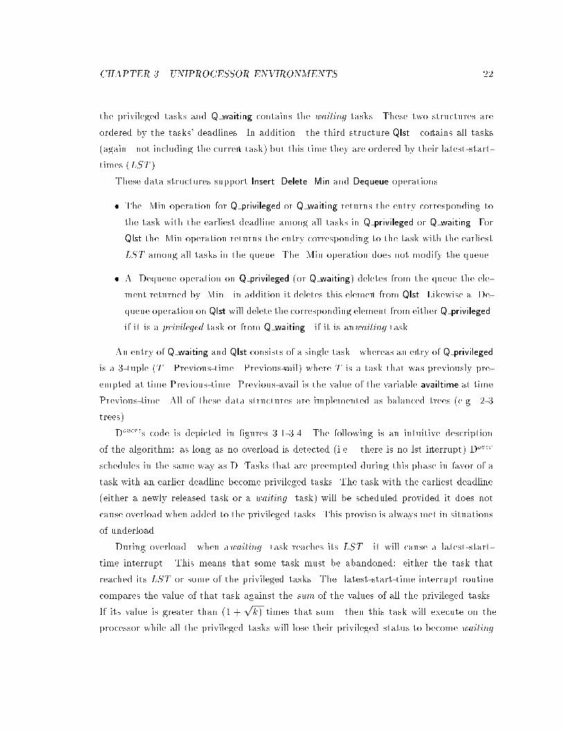
In the algorithm described below there are three kinds ofevents (each causing an associ-
ated interrupt) considered:
� Task Completion: successful termination of a task. This event has the highest priority.
� Task Release: arrival of a new task. This event has low priority.
� Latest-start-time Interrupt: the indication that a task must immediately be scheduled
in order to complete by its deadline that is the task's remaining computation time is
equal to the time remaining until its deadline. This event has also low priority (the
same as task release).
If several interrupts happen simultaneously they are handled according to their priori-
ties. A task completion interrupt is handled before the task release and latest-start-time
interrupt interrupts which are handled in random order. It may happen that a task com-
pletion event suppresses a lower priority interrupt e.g. the task completion handler
schedules the next task if this task had just reached its LST then the latest-start-time
interrupt is removed.
At any given moment the set of ready tasks1 is partitioned into two disjoint sets.
privileged tasks and waiting tasks. Whenever a task is preempted it becomes a privileged
task. However whenever some task is scheduled as a result of latest-start-time interrupt
all the ready tasks (whether preempted or never scheduled) become waiting tasks.
Dover maintains a special quantity called availtime. Suppose a new task is released into
the system and its deadline is the earliest among all ready tasks. The value of availtime
is the maximum computation time that can be taken by such a task without causing the
current task or any of the privileged tasks to miss their deadlines.
Dover requires three data structures calledQ privileged Q waiting and Qlst. Each entry
in these data structures corresponds to a task in the system. Q privileged contains exactly
1Excluding the currently executing task.
CHAPTER 3. UNIPROCESSOR ENVIRONMENTS 22
the privileged tasks and Q waiting contains the waiting tasks. These two structures are
ordered by the tasks' deadlines. In addition the third structure Qlst contains all tasks
(again not including the current task) but this time they are ordered by their latest-start-
times (LST ).
These data structures support Insert Delete Min and Dequeue operations.
� The Min operation for Q privileged or Q waiting returns the entry corresponding to
the task with the earliest deadline among all tasks in Q privileged or Q waiting. For
Qlst the Min operation returns the entry corresponding to the task with the earliest
LST among all tasks in the queue. The Min operation does not modify the queue.
� A Dequeue operation on Q privileged (or Q waiting) deletes from the queue the ele-
ment returned by Min in addition it deletes this element from Qlst. Likewise a De-
queue operation on Qlst will delete the corresponding element from either Q privileged
if it is a privileged task or from Q waiting if it is anwaiting task.
An entry of Q waiting and Qlst consists of a single task whereas an entry of Q privileged
is a 3-tuple (T Previous-time Previous-avail) where T is a task that was previously pre-
empted at time Previous-time. Previous-avail is the value of the variable availtime at time
Previous-time. All of these data structures are implemented as balanced trees (e.g. 2-3
trees).
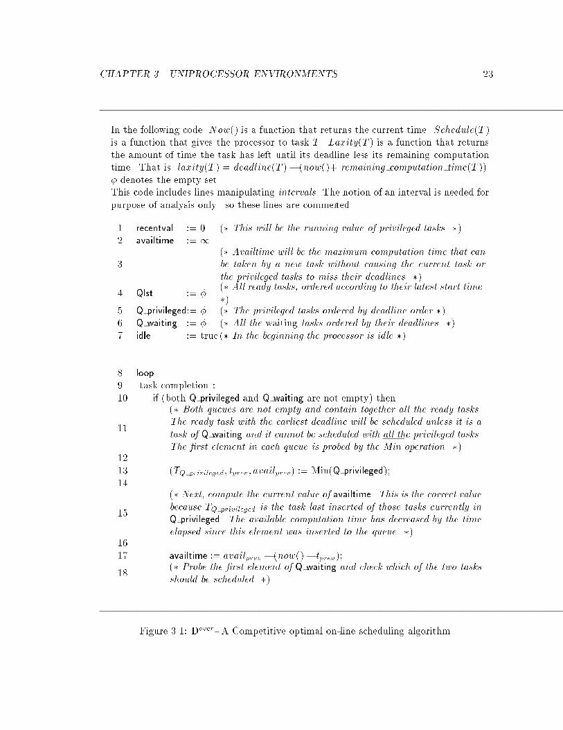
Dover's code is depicted in �gures 3.1-3.4. The following is an intuitive description
of the algorithm: as long as no overload is detected (i.e. there is no lst interrupt) Dover
schedules in the same way as D. Tasks that are preempted during this phase in favor of a
task with an earlier deadline become privileged tasks. The task with the earliest deadline
(either a newly released task or a waiting task) will be scheduled provided it does not
cause overload when added to the privileged tasks. This proviso is always met in situations
of underload.
During overload when awaiting task reaches its LST it will cause a latest-start-
time interrupt. This means that some task must be abandoned: either the task that
reached its LST or some of the privileged tasks. The latest-start-time interrupt routine
compares the value of that task against the sum of the values of all the privileged tasks.
If its value is greater than (1 +pk) times that sum then this task will execute on the
processor while all the privileged tasks will lose their privileged status to become waiting
CHAPTER 3. UNIPROCESSOR ENVIRONMENTS 23
In the following code Now() is a function that returns the current time. Schedule(T )is a function that gives the processor to task T . Laxity(T ) is a function that returnsthe amount of time the task has left until its deadline less its remaining computationtime. That is laxity(T ) = deadline(T )� (now()+ remaining computation time(T )).� denotes the empty set.This code includes lines manipulating intervals. The notion of an interval is needed forpurpose of analysis only so these lines are commented.
1 recentval := 0 (� This will be the running value of privileged tasks. �)2 availtime := 1
3(� Availtime will be the maximum computation time that can
be taken by a new task without causing the current task or
the privileged tasks to miss their deadlines. �)
4 Qlst := �(� All ready tasks, ordered according to their latest start time.
�)5 Q privileged:= � (� The privileged tasks ordered by deadline order �)6 Q waiting := � (� All the waiting tasks ordered by their deadlines. �)7 idle := true (� In the beginning the processor is idle �)
8 loop
9 task completion :10 if (both Q privileged and Q waiting are not empty) then
11
(� Both queues are not empty and contain together all the ready tasks.
The ready task with the earliest deadline will be scheduled unless it is a
task of Q waiting and it cannot be scheduled with all the privileged tasks.
The �rst element in each queue is probed by the Min operation. �)1213 (TQ privileged; tprev; availprev) := Min(Q privileged);14
15
(� Next, compute the current value of availtime. This is the correct value
because TQ privileged is the task last inserted of those tasks currently in
Q privileged. The available computation time has decreased by the time
elapsed since this element was inserted to the queue. �)1617 availtime := availprev � (now()� tprev);
18(� Probe the �rst element of Q waiting and check which of the two tasks
should be scheduled. �)
Figure 3.1: Dover- A Competitive optimal on-line scheduling algorithm.
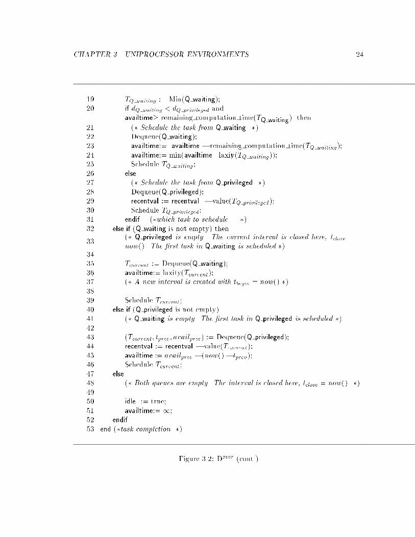
CHAPTER 3. UNIPROCESSOR ENVIRONMENTS 24
19 TQ waiting := Min(Q waiting);20 if dQ waiting < dQ privileged and
availtime� remaining computation time(TQ waiting) then
21 (� Schedule the task from Q waiting. �)22 Dequeue(Q waiting);23 availtime:= availtime � remaining computation time(TQ waiting);24 availtime:= min(availtime laxity(TQ waiting));25 Schedule TQ waiting;26 else
27 (� Schedule the task from Q privileged. �)28 Dequeue(Q privileged);29 recentval := recentval � value(TQ privileged);30 Schedule TQ privileged;31 endif (�which task to schedule. �)32 else if (Q waiting is not empty) then
33(� Q privileged is empty. The current interval is closed here, tclose =now(). The �rst task in Q waiting is scheduled �)
3435 Tcurrent := Dequeue(Q waiting);36 availtime:= laxity(Tcurrent);37 (� A new interval is created with tbegin = now().�)
3839 Schedule Tcurrent;40 else if (Q privileged is not empty)41 (� Q waiting is empty. The �rst task in Q privileged is scheduled �)4243 (Tcurrent; tprev; availprev) := Dequeue(Q privileged);44 recentval := recentval � value(Tcurrent);45 availtime := availprev � (now()� tprev);46 Schedule Tcurrent;47 else
48 (� Both queues are empty. The interval is closed here, tclose = now(). �)4950 idle := true;51 availtime:= 1;52 endif
53 end (�task completion �)
Figure 3.2: Dover (cont.)
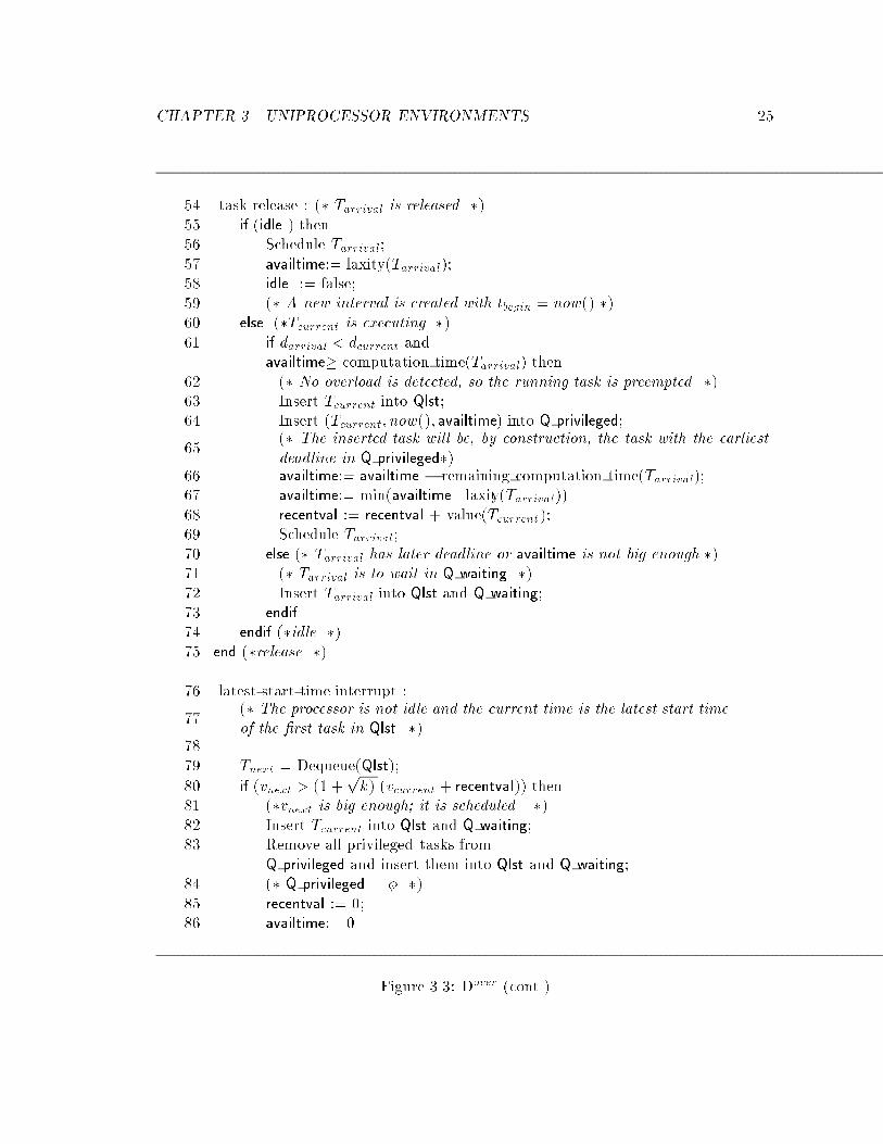
CHAPTER 3. UNIPROCESSOR ENVIRONMENTS 25
54 task release : (� Tarrival is released. �)55 if (idle ) then56 Schedule Tarrival;57 availtime:= laxity(Tarrival);58 idle := false;59 (� A new interval is created with tbegin = now().�)60 else (�Tcurrent is executing �)61 if darrival < dcurrent and
availtime� computation time(Tarrival) then62 (� No overload is detected, so the running task is preempted. �)63 Insert Tcurrent into Qlst;64 Insert (Tcurrent; now(); availtime) into Q privileged;
65(� The inserted task will be, by construction, the task with the earliest
deadline in Q privileged�)66 availtime:= availtime � remaining computation time(Tarrival);67 availtime:= min(availtime laxity(Tarrival))68 recentval := recentval + value(Tcurrent);69 Schedule Tarrival;70 else (� Tarrival has later deadline or availtime is not big enough.�)71 (� Tarrival is to wait in Q waiting �)72 Insert Tarrival into Qlst and Q waiting;73 endif
74 endif (�idle �)75 end (�release �)
76 latest-start-time interrupt :
77(� The processor is not idle and the current time is the latest start time
of the �rst task in Qlst. �)7879 Tnext = Dequeue(Qlst);
80 if (vnext > (1 +pk) (vcurrent + recentval)) then
81 (�vnext is big enough; it is scheduled. �)82 Insert Tcurrent into Qlst and Q waiting;83 Remove all privileged tasks from
Q privileged and insert them into Qlst and Q waiting;84 (� Q privileged = � �)85 recentval := 0;86 availtime:= 0
Figure 3.3: Dover (cont.)
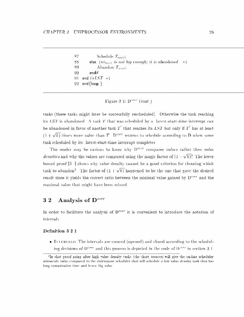
CHAPTER 3. UNIPROCESSOR ENVIRONMENTS 26
87 Schedule Tnext;88 else (�vnext is not big enough; it is abandoned. �)89 Abandon Tnext;90 endif
91 end (�LST �)92 endfloop g
Figure 3.4: Dover (cont.)
tasks (these tasks might later be successfully rescheduled). Otherwise the task reaching
its LST is abandoned. A task T that was scheduled by a latest-start-time interrupt can
be abandoned in favor of another task T0
that reaches its LST but only if T0
has at least
(1 +pk) times more value than T . Dover returns to schedule according to D when some
task scheduled by its latest-start-time interrupt completes.
The reader may be curious to know why Dover compares values rather then value
densities and why the values are compared using the magic factor of (1 +pk)? The lower
bound proof [3 4] shows why value density cannot be a good criterion for choosing which
task to abandon2. The factor of (1 +pk) happened to be the one that gave the desired
result since it yields the correct ratio between the minimal value gained by Dover and the
maximal value that might have been missed.
3.2 Analysis of Dover
In order to facilitate the analysis of Dover it is convenient to introduce the notation of
intervals.
De�nition 3.2.1
� Intervals: The intervals are created (opened) and closed according to the schedul-
ing decisions of Dover and this process is depicted in the code of Dover in section 3.1.
2In that proof going after high value density tasks (the short teasers) will give the on-line schedulerminuscule value compared to the clairvoyant scheduler that will schedule a low value density task that haslong computation time and hence big value.
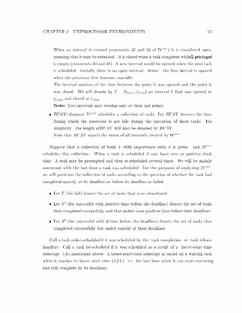
CHAPTER 3. UNIPROCESSOR ENVIRONMENTS 27
When an interval is created (comments 37 and 59 of Dover) it is considered open
meaning that it may be extended it is closed when a task completes whileQ privileged
is empty (comments 33 and 48). A new interval would be opened when the next task
is scheduled. Initially there is no open interval. Hence the �rst interval is opened
when the processor �rst becomes non-idle.
The interval consists of the time between the point it was opened and the point it
was closed. We will denote by I = [tbegin; tclose] an interval I that was opened at
tbegin and closed at tclose .
Note: Two intervals may overlap only at their end points.
� BUSY: Suppose Dover schedules a collection of tasks. Let BUSY denotes the time
during which the processor is not idle during the execution of these tasks. For
simplicity the length ofBUSY will also be denoted by BUSY .
Note that BUSY equals the union of all intervals created by Dover.
Suppose that a collection of tasks � with importance ratio k is given. and Dover
schedules this collection. When a task is scheduled it can have zero or positive slack
time. A task may be preempted and then re-scheduled several times. We will be mainly
concerned with the last time a task was scheduled. For the purposes of analyzing Dover
we will partition the collection of tasks according to the question of whether the task had
completed exactly at its deadline or before its deadline or failed.
� Let F (for fail) denote the set of tasks that were abandoned.
� Let Sp (for successful with positive time before the deadline) denote the set of tasks
that completed successfully and that ended some positive time before their deadlines.
� Let S0 (for successful with 0 time before the deadline) denote the set of tasks that
completed successfully but ended exactly at their deadlines.
Call a task order-scheduled if it was scheduled by the task completion or task release
handlers. Call a task lst-scheduled if it was scheduled as a result of a latest-start-time
interrupt. (As mentioned above a latest-start-time interrupt is raised on a waiting task
when it reaches its latest start time (LST ) i.e. the last time when it can start executing
and still complete by its deadline).
CHAPTER 3. UNIPROCESSOR ENVIRONMENTS 28
The �rst task in each interval is order-scheduled. The subsequent tasks (if any) in
this interval may be order-scheduled or lst-scheduled. Proposition 3.2.1 shows that once a
task is lst-scheduled all subsequent tasks of this interval must be lst-scheduled. During an
interval several order-scheduled tasks may complete but only one lst-scheduled task can
complete (this task will also be the last task that executes in the interval).
Proposition 3.2.1 According to the scheduling of Dover once a task is lst-scheduled, then
all subsequent tasks, in the current interval, are lst-scheduled.
proof.
Suppose the current task Tcurrent is lst-scheduled and a task Tarrival is released.Tarrival
will not be scheduled by the task release handler because when the current task is lst-
scheduled availtime equals zero (see statement 86 of Dover) hence no task can be scheduled
by the task release handler (see statement 61 of Dover).
Let recentval(t) denote3 recentval at time t and achievedvalue(t) denote4 the value
achieved during the current interval before t. For an interval I achievedvalue(I) is the
total value obtained during I .
We partition the value obtained during I in two di�erent ways:
� ordervalue vs. lstvalue: ordervalue(I) is the total value obtained by order-scheduled
tasks that completed during I . The value obtained by lst-scheduled tasks is denoted
by lstvalue(I) (there is at most one such task in any interval I).
� zerolaxval vs. poslaxval: zerolaxval(I) denotes the total value obtained by tasks that
completed at their deadlines during I (tasks in S0). The value obtained by tasks
that completed before their deadlines is denoted by poslaxval(I).
Hence for every interval
achievedvalue(I) = ordervalue(I) + lstvalue(I) = zerolaxval(I) + poslaxval(I)
When the index (I) is omitted we refer to the entire execution. For example ordervalue
denotes the total value obtained by order-scheduled tasks summing over all intervals.
3In the following only recentval is a variable explicitly manipulated by Dover. All the others:
zerolaxval; poslaxval; ordervalue and lstvalue are introduced here to facilitate the analysis. This
is why they do not reference algorithm statements.4See statements 1,29,44,68 and 85.
CHAPTER 3. UNIPROCESSOR ENVIRONMENTS 29
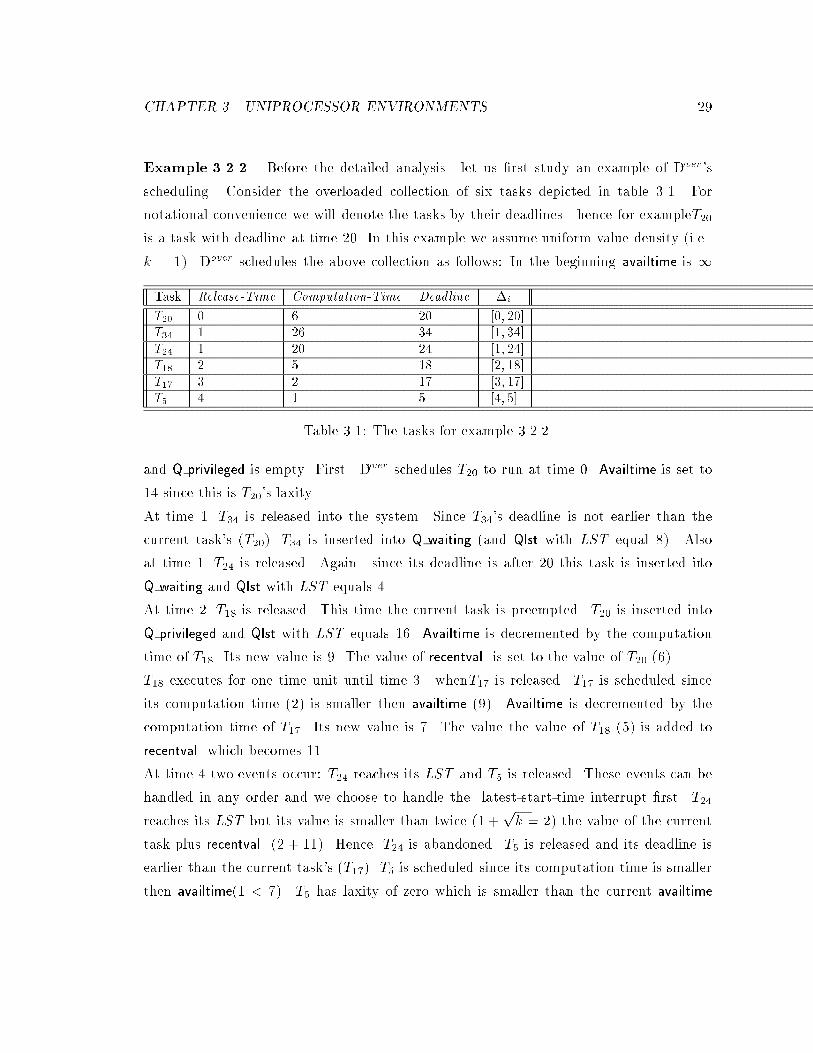
Example 3.2.2 Before the detailed analysis let us �rst study an example of Dover 's
scheduling. Consider the overloaded collection of six tasks depicted in table 3.1. For
notational convenience we will denote the tasks by their deadlines hence for exampleT20
is a task with deadline at time 20. In this example we assume uniform value density (i.e.
k = 1). Dover schedules the above collection as follows: In the beginning availtime is 1
Task Release-Time Computation-Time Deadline �i
T20 0 6 20 [0; 20]T34 1 26 34 [1; 34]
T24 1 20 24 [1; 24]T18 2 5 18 [2; 18]
T17 3 2 17 [3; 17]T5 4 1 5 [4; 5]
Table 3.1: The tasks for example 3.2.2.
and Q privileged is empty. First Dover schedules T20 to run at time 0. Availtime is set to
14 since this is T20's laxity.
At time 1 T34 is released into the system. Since T34's deadline is not earlier than the
current task's (T20) T34 is inserted into Q waiting (and Qlst with LST equal 8). Also
at time 1 T24 is released. Again since its deadline is after 20 this task is inserted into
Q waiting and Qlst with LST equals 4.
At time 2 T18 is released. This time the current task is preempted. T20 is inserted into
Q privileged and Qlst with LST equals 16. Availtime is decremented by the computation
time of T18. Its new value is 9. The value of recentval is set to the value of T20 (6).
T18 executes for one time unit until time 3 whenT17 is released. T17 is scheduled since
its computation time (2) is smaller then availtime (9). Availtime is decremented by the
computation time of T17. Its new value is 7. The value the value of T18 (5) is added to
recentval which becomes 11.
At time 4 two events occur: T24 reaches its LST and T5 is released. These events can be
handled in any order and we choose to handle the latest-start-time interrupt �rst. T24
reaches its LST but its value is smaller than twice (1 +pk = 2) the value of the current
task plus recentval (2 + 11). Hence T24 is abandoned. T5 is released and its deadline is
earlier than the current task's (T17). T5 is scheduled since its computation time is smaller
then availtime(1 < 7). T5 has laxity of zero which is smaller than the current availtime
CHAPTER 3. UNIPROCESSOR ENVIRONMENTS 30
minus the computation time of T5 (6). Hence availtime is now set to 0 and recentval
becomes 11 + 2 = 13.
At time 5 T5 completes and since T17 is the task with the earliest deadline it is scheduled.
Availtime is now 6 because this the value of availtime when T17 was executing (7) minus
the time elapsed since it was inserted to Q privileged (1). The value of T17 is subtracted
from recentval which becomes 13� 2 = 11.
The remaining computation time of T17 is one unit hence at time 6 it completes. The next
task in Q privileged is T18 which has a remaining computation time of 4 units. Availtime
is set to 6 which is value of availtime when T18 was executing (9) minus the time elapsed
since it was inserted to Q privileged ((6 � 3) = 3) (the value of T18 is subtracted from
recentval which becomes 11 � 5 = 6). However T18 will execute only until 8 when T34
reaches its LST . The value of T34 is big enough to preempt the current task. All tasks
from Q privileged are moved to Q waiting and availtime as well as recentval are reset to
zero.
The LST of T18 is 16 and of T20 (the only other task in Qlst) is 15. These tasks will
generate latest-start-time interrupt in these respective times both will be abandoned.
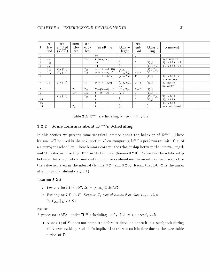
At time 34 T34 completes its execution and Dover �nished scheduling this history. Table 3.2
summarizes the scheduling decisions of Dover. In this example S0 = [T5; T34]; Sp = [T17]
and F = [T18; T20; T24]. Only three tasks complete their execution and the total value
obtained by Dover is 29. A clairvoyant scheduler can achieve a value of 34 by scheduling
T17; T20 and T34. Also notice that the system is already overloaded at time 1 but the �rst
time an overload is \detected" by Dover is at time 4.
3.2.1 Proof Strategy
Our goal is to show that Dover has a competitive multiplier of (1 +pk)2 for every collection
of tasks with importance ratio of k. We will start by proving some lemmas about the
behavior of Dover . Then we will try to estimate the best possible behavior of a clairvoyant
algorithm by comparison to Dover . Our basic strategy is to bound from below what Dover
achieves during each interval. This will lead to a global lower bound over the entire
execution. Then we bound from above what a clairvoyant scheduler can achieve during
the entire execution.
CHAPTER 3. UNIPROCESSOR ENVIRONMENTS 31
re- pre- com- sch- rec-t lea- empted ple- edu- availtime Q priv- ent- Q wait comment
sed (LST ) ted led ileged val ing0 1 [] 0 []0 T20 T20 laxity(T20) [] 0 [] new interval1 T34 14 [] 0 [T34] T34's LST is 81 T24 14 [] 0 [T24; T34] T24's LST is 42 T18 T20 (16) T18 min(14� 5; 13) [T20] 6 [T24; T34]3 T17 T18 (14) T17 min(9� 2;12) [T18; T20] 5 + 6 [T24; T34]4 min(9� 2;12) [T18; T20] 11 [T34] T24's LST , it
is abandoned4 T5 T17 (16) T5 min(7� 1;0) [T17; T18; 2 + 11 [T34] T5 has no
T20] no laxity5 T5 T17 7� (5� 4) = 6 [T18; T20] 5 + 6 [T34]6 T17 T18 9� (6� 3) = 6 [T20] 6 [T34]8 T18 (15) T34 0 [] 0 [T18; T20] T34`s LST15 0 [] 0 [T18] T20's LST16 0 [] 0 [] T18's LST34 T34 0 [] [] interval closed
Table 3.2: Dover's scheduling for example 3.2.2.
3.2.2 Some Lemmas about Dover's Scheduling
In this section we present some technical lemmas about the behavior of Dover. These
lemmas will be used in the next section when comparing Dover 's performance with that of
a clairvoyant scheduler. These lemmas concern the relationship between the interval length
and the value achieved by Dover in that interval (lemma 3.2.3). As well as the relationship
between the computation time and value of tasks abandoned in an interval with respect to
the value achieved in the interval (lemma 3.2.4 and 3.2.5). Recall that BUSY is the union
of all intervals (de�nition 3.2.1).
Lemma 3.2.2
1. For any task Ti in S0, �i = [ri; di] � BUSY
2. For any task Ti in F . Suppose Ti was abandoned at time taban, then
[ri; taban] � BUSY
proof.
A processor is idle under Dover scheduling only if there is noready task.
� A task Ti of S0 does not complete before its deadline hence it is a ready task during
all its executable period. This implies that there is no idle time during the executable
period of Ti.
CHAPTER 3. UNIPROCESSOR ENVIRONMENTS 32
� Similarly a task ofF is a ready task from its release time to the point at which
it is abandoned. Therefore there is no idle time between its release point and its
abandonment point.
Lemma 3.2.3 For any interval I = [tbegin; tclose], the length of I, tclose� tbegin will satisfy
tclose � tbegin � ordervalue(I) + (1 +1pk) � lstvalue(I)
= achievedvalue(I) +1pk� lstvalue(I)
Recall that ordervalue(I) and lstvalue(I) are the values obtained by Dover from the order-
scheduled and the lst-scheduled tasks respectively during I.
proof.
An interval I = [tbegin; tclose] has the following two sub-portions the second of which may
be empty:
1. [tbegin; tfirst lst]
From the beginning of I to the point in time tfirst lst in which the �rst lst-scheduled
task is scheduled. During this period all tasks are order-scheduled and some may
complete their execution.
If no task is lst-scheduled in I then de�ne tfirst lst to be tclose . In this case the second
sub-portion is empty.
2. [tfirst lst; tclose]
During this period all tasks are scheduled and preempted by latest-start-time in-
terrupt. Only the last task to be scheduled completes.
If there are no lst-scheduled tasks in I then all tasks that executed from tbegin to tclose
completed successfully. The value achieved is ordervalue(I) and is at least as big as the
duration of execution5. Hence the lemma is proved in this case.
Otherwise suppose thatT1; T2; � � � ; Tm (m � 1) are the tasks that were lst-scheduled in
I . Hence T1 was scheduled at tfirst lst later it was preempted (and abandoned) by T2 and
so forth. Eventually Tm preempts Tm�1 and completes at tclose its value vm is lstvalue(I).
5Recall that a value density is always equal or greater than 1, by assumption 2.0.2 above.
CHAPTER 3. UNIPROCESSOR ENVIRONMENTS 33
Denote by li the length of the execution of Ti during the process above. Tm preempted
Tm�1 hence vm > (1 +pk)vm�1. Which yields6
lm�1 < vm�1 <vm
(1 +pk)
=lstvalue(I)
(1 +pk)
Going backward along the chain of preemptions we get:
li < vi <vi�1
(1 +pk)
<lstvalue(I)
(1 +pk)m�i
for all 1 � i � m� 1 (3.1)
T1 preempted the last order-scheduled task hence (see statement 80 of Dover)
v1 > (1 +pk)frecentval(tfirst lst) + value(current task at time tfirst lst)g (3.2)
Also
tfirst lst � tbegin � ordervalue(I) + recentval(tfirst lst)+
value(current task at time tfirst lst) (3.3)
This holds because the processor is not idle between tbegin and tfirst lst (as part of BUSY )
and the right hand side above represents the sum of the values of all the tasks that were
scheduled between tbegin and tfirst lst. This sum must be greater than or equal to their
period of execution by the normalized importance assumption (assumption 2.0.2). Inequal-
ities 3.1 3.2 and 3.3 imply
tfirst lst � tbegin < ordervalue(I) +v1
(1 +pk)
< ordervalue(I) +lstvalue(I)
(1 +pk)m
We have produced the following bound on the distance between tbegin and tclose:
tclose � tbegin = (tfirst lst � tbegin) + (tclose � tfirst lst)
= (tfirst lst � tbegin) + (l1 + l2 + � � �+ lm)
� ordervalue(I) +
lstvalue(I) � 1 +
1
(1 +pk)
+1
(1 +pk)2
+ � � �+ 1
(1 +pk)m
!
� ordervalue(I) + lstvalue(I) �1Xi=0
1
(1 +pk)i
= ordervalue(I) + lstvalue(I) � (1 + 1pk)
= achievedvalue(I) +1pk� lstvalue(I)
6Note that always li � vi. However, for a task that was abandoned a strict inequality li < vi holds.
CHAPTER 3. UNIPROCESSOR ENVIRONMENTS 34
The last equality follows from the fact that achievedvalue(I) = ordervalue(I) + lstvalue(I)
by de�nition.
Lemma 3.2.4 Suppose Ti was abandoned during the interval I. Then
vi � (1 +pk) � achievedvalue(I)
Recall that achievedvalue(I) is the total value obtained during I.
proof.
Let I = [tbegin; tclose] be an interval. De�ne the Prospective Valuemap of I PVI as follows:
PVI(t) = ordervalue(t) + recentval(t) + value(current task at time t)
where tbegin � t � tclose
Claim For every interval I = [tbegin; tclose]
1. PVI is monotone non-decreasing.
2. PVI reaches at the end of the interval the total value obtained in I i.e
PVI(tclose) = achievedvalue(I)
Note: PV is not a function because it might have several values for one time instance
since Dover can make several scheduling decisions at one time instance (assumption 2.0.2).
However as a map with the ordered sequence of scheduling decisions as its domain PVI
is a function.
Proof of claim.
There are two cases. The �rst applies when there are no lst-scheduled tasks in I the other
applies when such tasks exist.
Case 1: Suppose that there are no lst-scheduled tasks in I . Then every task that was
scheduled does complete. Let S(t) be the set of tasks that were scheduled (not necessary
completed) up to t. One can verify by induction that
PVI(t) =X
Ti2S(t)
vi
The reason is that no scheduled task is abandoned hence at each moment a task is either
the current task or in Q privileged or had completed. At the closing of I all tasks have
CHAPTER 3. UNIPROCESSOR ENVIRONMENTS 35
completed. Hence
PVI(tclose) =X
Ti2S(tclose)
vi = achievedvalue(I)
PVI is monotone (when there are no lst-scheduled tasks) because S(t) is a monotone
increasing set of tasks.
Case 2: Suppose there were lst-scheduled tasks. Assume that the �rst lst-scheduled task
T1 was scheduled at time tfirst lst. Let t be a time instance just before the scheduling of
T1 then by de�nition:
PVI(t) = ordervalue(t) + recentval(t) + value(current task at time t)
T1 is scheduled only if
v1 > (1 +pk) � (recentval(t) + value(current task at time t))
When T1 is scheduled recentval is set to zero hence we can conclude that
PVI(tfirst lst) = ordervalue(tfirst lst) + recentval(tfirst lst) + value(T1)
= ordervalue(t) + 0 + value(T1)
> ordervalue(t) + (recentval(t) + value(current task at time t))
= PVI(t)
Thus PVI is monotone from tbegin to tfirst lst (as in the case when there are no lst-scheduled
tasks). It is left to show that PVI continues to be monotone. After tfirst lst PVI equals
to
ordervalue(I) + value(current task at time t)
because recentval remains equal to zero. This is a monotone increasing value since ordervalue(I)
is �xed and a task T will preempt the current task only if it has a larger value than the
current task's value. In particular if Ti is the last task to be scheduled in I then
PVI = ordervalue(I) + vi
= ordervalue(I) + lstvalue(I) = achievedvalue(I)
So the claim is proved.
CHAPTER 3. UNIPROCESSOR ENVIRONMENTS 36
End of proof of claim
We return to the proof of lemma 3.2.4. There is only one way a task Ti can be
abandoned at time t:
� Ti reaches its LST at t. A latest-start-time interrupt is generated. However Ti has
insu�cient value to preempt the task executing at time t.
Hence if Ti was abandoned then
vi < (1 +pk) � frecentval(t) + value(current task at time t)g
� (1 +pk) � PVI(t) ; by de�nition of PV
� (1 +pk) � achievedvalue(I) ; by the claim
Lemma 3.2.5 Suppose Ti was abandoned at time t in I = [tbegin; tclose]. Then,
ci � di � tclose
proof.
A task Ti can be abandoned at timet only when:
� It reaches its LST at t. A latest-start-time interrupt is generated. However the
current task is not preempted.
Ti reached its LST hence its remaining computation time is di � t. Also t � tclose by
assumption. Hence the (initial) computation time of Ti is at least di � tclose .
3.2.3 How Well Can a Clairvoyant Scheduler Do?
Given a collection of tasks � our goal is to bound the maximum value that a clairvoyant
algorithm can obtain from scheduling �. We do it by observing the way Dover schedules
�. From Dover 's scheduling we get the partitioning of the tasks to S0; Sp and F we also
take notice of the time periods in which the processor was not idle in this scheduling. As
de�ned earlier the union of these periods is calledBUSY .
In order to bound the value that can be achieved from scheduling � we will o�er the
clairvoyant algorithm two gifts that can only improve the value it can obtain. We will
CHAPTER 3. UNIPROCESSOR ENVIRONMENTS 37
show an upper bound on the value the clairvoyant algorithm can get with these gifts hence
bounding the value it can achieve from the original collection.
� As a �rst gift we will give the clairvoyant algorithm the sum of the values of all tasks
in Sp at no cost to it (i.e. it will devote no time to these tasks). Then we will see
what the clairvoyant algorithm can achieve on F [ S0.
� As a second gift suppose that in addition to the value achieved from scheduling the
tasks F[S0 the clairvoyant scheduler can get an additional value called granted value.
The amount of granted value depends on the schedule chosen by the the clairvoyant
scheduler: A value density of k will be granted for every period of BUSY that is not
used for executing a task.
The clairvoyant scheduler must consider that scheduling a task might reduce the granted
value (since time in BUSY is used). Of course when this reduction is bigger than the
value of a task then the task should not be scheduled. Suppose the clairvoyant algorithm
had chosen a scheduling for F [ S0. We can assume that no task was scheduled entirely
during BUSY because the granted value lost would be greater or equal to the value gained
from scheduling the task. We will show that tasks of S0 can execute only during BUSY
hence this leaves only tasks of F that were scheduled partially7 outside BUSY . Executing
T results in a gain of value(T ) but entails a loss of the granted value for the time that T
executed in BUSY .
The clairvoyant scheduler has now two options. It can schedule no task during the
entire BUSY period and get only (the whole) granted value or it can use some of BUSY
in order to schedule some of F tasks. We will show that the maximal possible gain from
choosing the second option over the �rst is bounded by (1 +pk) � achievedvalue. Putting
this altogether will give the desired result (theorem 3.2.12).
Example 3.2.3 To see the possibilities opened to the clairvoyant algorithm by intro-
ducing the granted value consider the following example: The length of BUSY is 5 and
the importance ratio k is 4.F contains only one task T with computation length 3 and
value density 2. Without scheduling T the value obtained by the clairvoyant algorithm
7When the computation time of a task is known precisely when it is released, a task T 2 F cannot bescheduled completely outside BUSY (see lemma 3.2.2). However, if the computation time of a task is notexactly known (appendix C), then a failed task T may be scheduled completely outside BUSY .
CHAPTER 3. UNIPROCESSOR ENVIRONMENTS 38
only from the granted value is 5 � 4 = 20. If T could have been scheduled without using
any of BUSY time then its value will be added to give 20 + 2 � 3 = 26. However if the
clairvoyant algorithm must use 2 units of BUSY 's time in order to schedule T then the
total value will be only (5� 2)� 4 + 6 = 18 hence it is better not to schedule T in this
case. As a matter of fact whenever T has to use more than 1:5 units of BUSY 's time it
should not be scheduled.
In the scenario above the clairvoyant scheduler can achieve (using the gifts) the maximal
value of the sum in equation 3.4 below ranging over all possible schedulings8 of F .
value obtained from those
tasks of F that were scheduled+ k �
length of time in BUSY not utilized to
schedule the tasks of F(3.4)
Denote by C(�) the value that a clairvoyant algorithm can achieve from a collection of
tasks. We would like to show that C(F [ S0) cannot be greater then this maximal value.
This will then give us an upper bound on what a clairvoyant algorithm can achieve.
Lemma 3.2.6
C(F [ S0) � max
possible
scheduling
of F
8>>>>><>>>>>:
value obtained by
scheduling tasks of
F
+ k �length of time in BUSY not
utilized by tasks of F
9>>>>>=>>>>>;
proof.
C(F [ S0) = max
8>><>>:
value obtained from
scheduling tasks of F+value obtained from scheduling tasks of S0
during the time not used by tasks of F
9>>=>>;
8Suppose a clairvoyant scheduler has to schedule a collection of tasks A. We can assume that it schedules
a task only if that task eventually completes. Hence the work of a clairvoyant scheduler is �rst to choose
the set of tasks A0� A that will be scheduled and then to work out the details of the processor allocation
among the tasks of A0. We will call all possible selections of A0 and processor allocation a scheduling of A.
CHAPTER 3. UNIPROCESSOR ENVIRONMENTS 39
S0 tasks can be scheduled only during BUSY (lemma 3.2.2) hence
value obtained from
scheduling tasks of F+
value obtained from scheduling tasks of S0
during the time not used by tasks of F
�value obtained by
scheduling F+ k � length of time in BUSY not utilized
by tasks of F
The lemma is proved.
With the above gifts the clairvoyant scheduler can maximize the sum in 3.4 above
and hence obtain a value of at least C(F [ S0).
Suppose a task Tf 2 F is scheduled to completion by the clairvoyant algorithm. If Tf
executes entirely during BUSY then the left hand factor of the sum is increased only by
vi which is smaller than or equal to k � ci while the right hand factor is decreased by k � cigiving zero or negative net change. Thus we assume that Tf executes (at least partially)
outside BUSY .
Lemma 3.2.7 Suppose Tf is abandoned (by Dover) at time taban and that I = [tbegin; tclose]
is the interval in which Tf is abandoned. Then, if Tf is to be executed (by the clairvoyant
algorithm) anywhere outside BUSY it must be after tclose.
proof.
�f = [rf ; taban][ [taban; df ]. The �rst portion of �f is contained in BUSY (lemma 3.2.2).
[taban; tclose] � I � BUSY hence ifTi is to be scheduled anywhere outside BUSY it must
be after tclose 9.
Now we are ready to give an upper bound on how much additional value can the clairvoyant
algorithm achieve by scheduling tasks of F compared with collecting only the granted
value without scheduling any tasks. We make strong use of the fact that when a task T is
abandoned during I T 's value cannot be too large with respect to achievedvalue(I).
Lemma 3.2.8 With the above gifts, the total net gain obtained by the clairvoyant algo-
rithm from scheduling the tasks abandoned during I is not greater than
(1 +pk) � achievedvalue(I)
9Note that parts of [tclose; df ] might be included in BUSY as a new interval may be opened before df
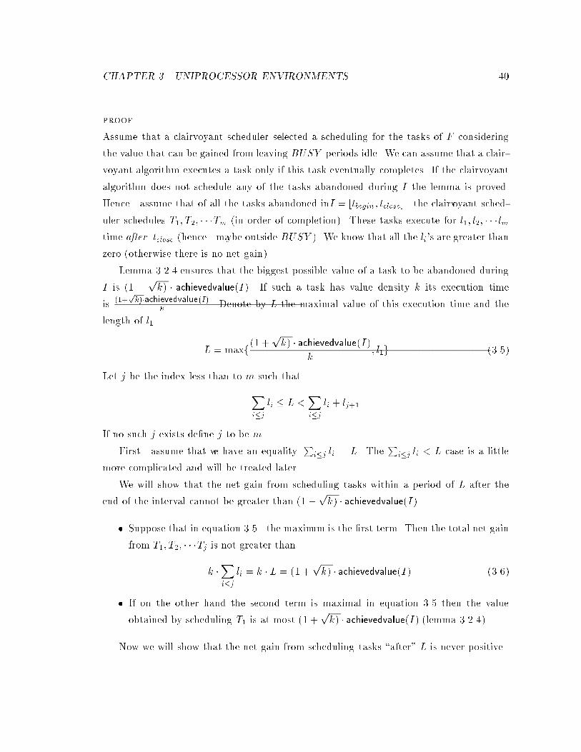
CHAPTER 3. UNIPROCESSOR ENVIRONMENTS 40
proof.
Assume that a clairvoyant scheduler selected a scheduling for the tasks of F considering
the value that can be gained from leaving BUSY periods idle. We can assume that a clair-
voyant algorithm executes a task only if this task eventually completes. If the clairvoyant
algorithm does not schedule any of the tasks abandoned during I the lemma is proved.
Hence assume that of all the tasks abandoned inI = [tbegin; tclose] the clairvoyant sched-
uler schedules T1; T2; � � �Tm (in order of completion). These tasks execute for l1; l2; � � �lmtime after tclose (hence maybe outside BUSY ). We know that all the li's are greater than
zero (otherwise there is no net gain).
Lemma 3.2.4 ensures that the biggest possible value of a task to be abandoned during
I is (1 +pk) � achievedvalue(I). If such a task has value density k its execution time
is(1+
pk)�achievedvalue(I)
k. Denote by L the maximal value of this execution time and the
length of l1
L = maxf(1 +pk) � achievedvalue(I)
k; l1g (3.5)
Let j be the index less than to m such that
X
i�j
li � L <X
i�j
li + lj+1
If no such j exists de�ne j to be m.
First assume that we have an equalityP
i�j li = L. TheP
i�j li < L case is a little
more complicated and will be treated later.
We will show that the net gain from scheduling tasks within a period of L after the
end of the interval cannot be greater than (1 +pk) � achievedvalue(I).
� Suppose that in equation 3.5 the maximum is the �rst term. Then the total net gain
from T1; T2; � � �Tj is not greater than
k �X
i�j
li = k � L = (1 +pk) � achievedvalue(I) (3.6)
� If on the other hand the second term is maximal in equation 3.5 then the value
obtained by scheduling T1 is at most (1 +pk) � achievedvalue(I) (lemma 3.2.4).
Now we will show that the net gain from scheduling tasks \after" L is never positive.
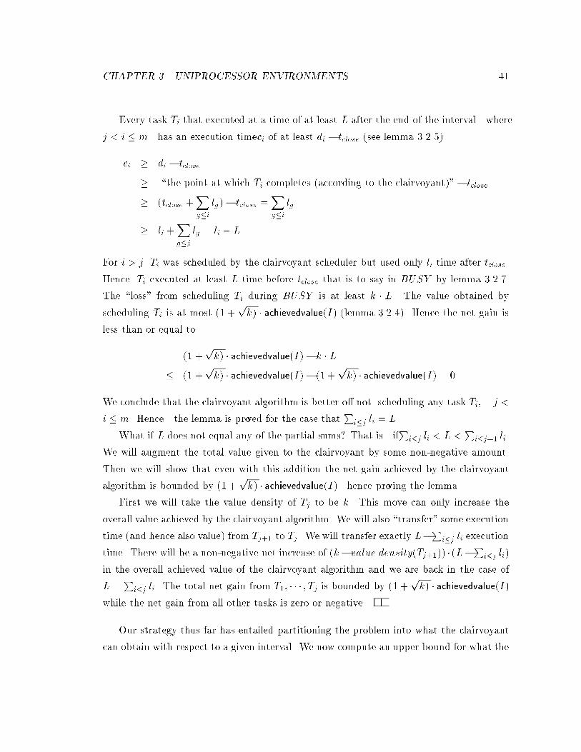
CHAPTER 3. UNIPROCESSOR ENVIRONMENTS 41
Every task Ti that executed at a time of at least L after the end of the interval where
j < i � m has an execution timeci of at least di � tclose (see lemma 3.2.5).
ci � di � tclose
� \the point at which Ti completes (according to the clairvoyant)"� tclose
� (tclose +X
g�i
lg)� tclose =X
g�i
lg
� li +X
g�j
lg = li + L
For i > j Ti was scheduled by the clairvoyant scheduler but used only li time after tclose .
Hence Ti executed at least L time before tclose that is to say in BUSY by lemma 3.2.7.
The \loss" from scheduling Ti during BUSY is at least k � L. The value obtained by
scheduling Ti is at most (1 +pk) � achievedvalue(I) (lemma 3.2.4). Hence the net gain is
less than or equal to
(1 +pk) � achievedvalue(I)� k � L
� (1 +pk) � achievedvalue(I)� (1 +
pk) � achievedvalue(I) = 0
We conclude that the clairvoyant algorithm is better o� not scheduling any task Ti; j <
i � m. Hence the lemma is proved for the case thatP
i�j li = L.
What if L does not equal any of the partial sums? That is ifP
i�j li < L <P
i�j+1 li.
We will augment the total value given to the clairvoyant by some non-negative amount.
Then we will show that even with this addition the net gain achieved by the clairvoyant
algorithm is bounded by (1 +pk) � achievedvalue(I) hence proving the lemma.
First we will take the value density of Tj to be k. This move can only increase the
overall value achieved by the clairvoyant algorithm. We will also \transfer" some execution
time (and hence also value) from Tj+1 to Tj . We will transfer exactly L�Pi�j li execution
time. There will be a non-negative net increase of (k� value density(Tj+1)) � (L�P
i�j li)
in the overall achieved value of the clairvoyant algorithm and we are back in the case of
L =P
i�j li. The total net gain from T1; � � � ; Tj is bounded by (1 +pk) � achievedvalue(I)
while the net gain from all other tasks is zero or negative.
Our strategy thus far has entailed partitioning the problem into what the clairvoyant
can obtain with respect to a given interval. We now compute an upper bound for what the
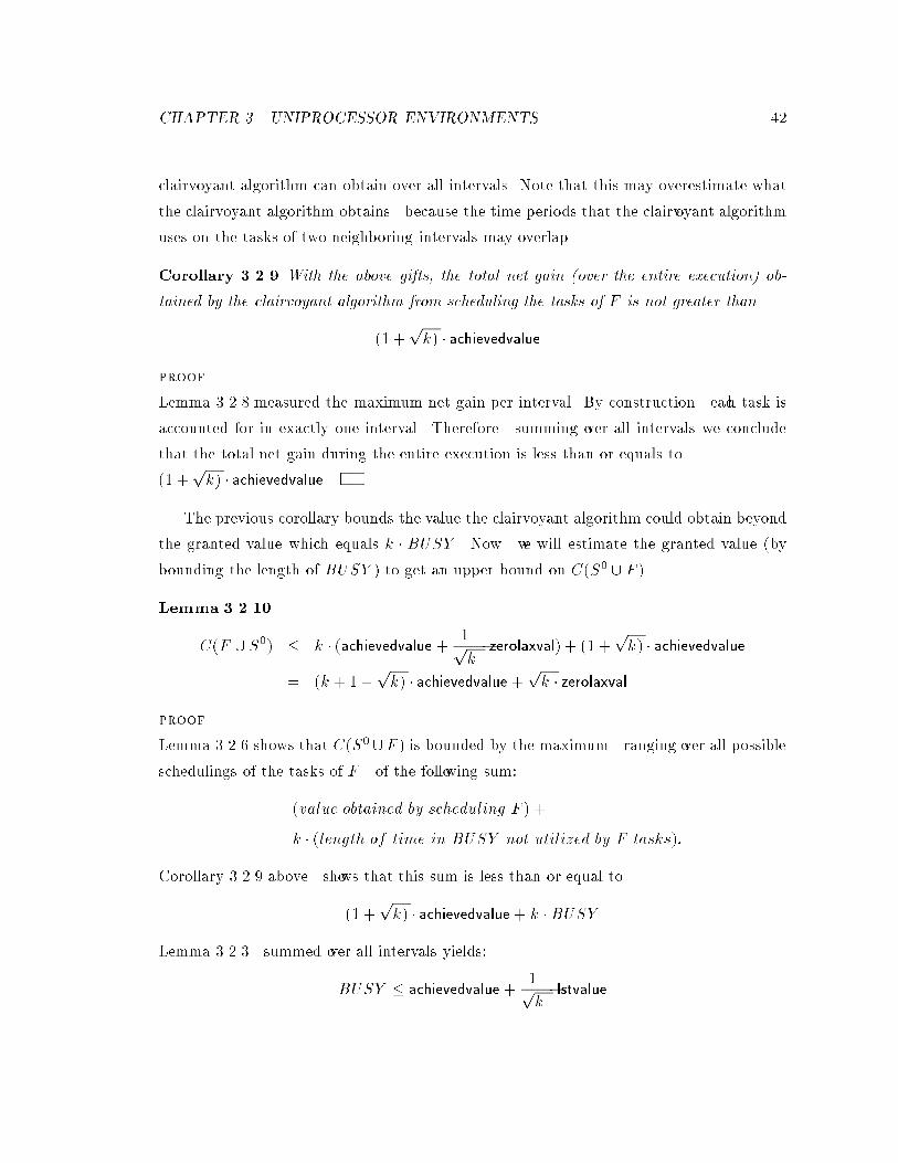
CHAPTER 3. UNIPROCESSOR ENVIRONMENTS 42
clairvoyant algorithm can obtain over all intervals. Note that this may overestimate what
the clairvoyant algorithm obtains because the time periods that the clairvoyant algorithm
uses on the tasks of two neighboring intervals may overlap.
Corollary 3.2.9 With the above gifts, the total net gain (over the entire execution) ob-
tained by the clairvoyant algorithm from scheduling the tasks of F is not greater than
(1 +pk) � achievedvalue
proof.
Lemma 3.2.8 measured the maximum net gain per interval. By construction each task is
accounted for in exactly one interval. Therefore summing over all intervals we conclude
that the total net gain during the entire execution is less than or equals to
(1 +pk) � achievedvalue.
The previous corollary bounds the value the clairvoyant algorithm could obtain beyond
the granted value which equals k � BUSY . Now we will estimate the granted value (by
bounding the length of BUSY ) to get an upper bound on C(S0 [ F ).
Lemma 3.2.10
C(F [ S0) � k � (achievedvalue + 1pk� zerolaxval) + (1 +
pk) � achievedvalue
= (k + 1+pk) � achievedvalue +
pk � zerolaxval
proof.
Lemma 3.2.6 shows that C(S0 [F ) is bounded by the maximum ranging over all possible
schedulings of the tasks of F of the following sum:
(value obtained by scheduling F ) +
k � (length of time in BUSY not utilized by F tasks):
Corollary 3.2.9 above shows that this sum is less than or equal to
(1 +pk) � achievedvalue + k �BUSY
Lemma 3.2.3 summed over all intervals yields:
BUSY � achievedvalue +1pk� lstvalue
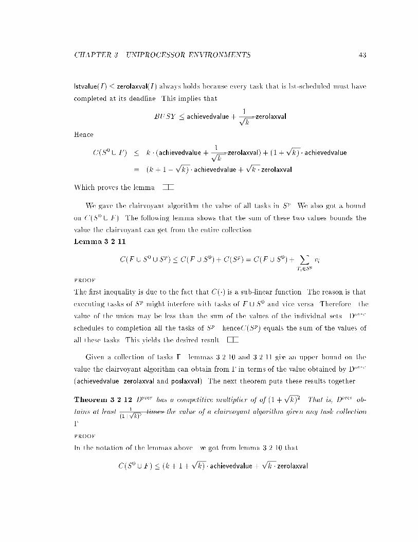
CHAPTER 3. UNIPROCESSOR ENVIRONMENTS 43
lstvalue(I) � zerolaxval(I) always holds because every task that is lst-scheduled must have
completed at its deadline. This implies that
BUSY � achievedvalue +1pk� zerolaxval
Hence
C(S0 [ F ) � k � (achievedvalue + 1pk� zerolaxval) + (1 +
pk) � achievedvalue
= (k + 1+pk) � achievedvalue +
pk � zerolaxval
Which proves the lemma.
We gave the clairvoyant algorithm the value of all tasks in Sp. We also got a bound
on C(S0 [ F ). The following lemma shows that the sum of these two values bounds the
value the clairvoyant can get from the entire collection.
Lemma 3.2.11
C(F [ S0 [ Sp) � C(F [ S0) + C(Sp) = C(F [ S0) +X
Ti2Sp
vi
proof.
The �rst inequality is due to the fact that C(�) is a sub-linear function. The reason is that
executing tasks of Sp might interfere with tasks of F [ S0 and vice versa. Therefore the
value of the union may be less than the sum of the values of the individual sets. Dover
schedules to completion all the tasks of Sp henceC(Sp) equals the sum of the values of
all these tasks. This yields the desired result.
Given a collection of tasks � lemmas 3.2.10 and 3.2.11 give an upper bound on the
value the clairvoyant algorithm can obtain from � in terms of the value obtained by Dover
(achievedvalue zerolaxval and poslaxval). The next theorem puts these results together.
Theorem 3.2.12 Dover has a competitive multiplier of of (1 +pk)2. That is, Dover ob-
tains at least 1(1+
pk)2
times the value of a clairvoyant algorithm given any task collection
�.
proof.
In the notation of the lemmas above we got from lemma 3.2.10 that
C(S0 [ F ) � (k + 1+pk) � achievedvalue +
pk � zerolaxval
CHAPTER 3. UNIPROCESSOR ENVIRONMENTS 44
We will boundpk � zerolaxval in the above equation.
pk � achievedvalue =
pk � zerolaxval+
pk � poslaxval �
pk � zerolaxval+ poslaxval
)pk � zerolaxval �
pk � achievedvalue � poslaxval
Hence replacing (pk � zerolaxval) by (
pk � achievedvalue � poslaxval) yields:
C(S0 [ F ) � (k + 1+pk) � achievedvalue +
pk � achievedvalue � poslaxval
= (1 +pk)2 � achievedvalue � poslaxval
Using lemma 3.2.11 we get:
C(F [ S0 [ Sp) � C(F [ S0) + C(Sp)
= C(F [ S0) + poslaxval
� ((1 +pk)2 � achievedvalue � poslaxval) + poslaxval
= (1 +pk)2 � achievedvalue
3.2.4 The Running Complexity of Dover
In the previous section we analyzed the performance of Dover in the sense of what value
it will achieve from scheduling tasks to completion. In this section we study the cost of
executing the scheduling algorithm itself.
Theorem 3.2.13 If n bounds the number of unscheduled tasks in the system at any instant
then each task incurs an O(logn) amortized cost.
proof.
Dover requires three data structures calledQ privileged Q waiting and Qlst all of them
priority queues implemented as balanced search trees e.g. 2-3 trees. They supportInsert
Delete Min and Dequeue operations each taking O(logn) time for a queue with n tasks.
The structures share their leaf nodes which represent tasks.
Dover consists of a main loop with three \interrupt handlers" within it. The total
number of operations is dominated by the number of times each of these handler clauses
is executed and the number of data structure operations in each clause.
CHAPTER 3. UNIPROCESSOR ENVIRONMENTS 45
Suppose a history of m tasks is given. First let us estimate the number of times each
handler clause can be executed. A task during its lifetime causes exactly one task release
event and at most one task completion event as well as at most one latest-start-time
interrupt event. Hence while scheduling m tasks the total number of events is bounded
by 3m.
Now we will bound the number of queue operations in each handler clause.
� In the handler for the task release event (statement 54) there is a constant number
of queue operations. Hence this contributes a total of O(m) queue operations during
the entire history.
� In the handler for the task completion event (statement 9) there is a constant number
of queue operations. Hence this contributes a total of O(m) queue operations during
the entire history.
� In the handler for latest-start-time interrupt event (see statement 76) the number
of queue operations is proportional to the number of tasks in Q privileged plus a
constant (because the privileged tasks are all inserted into Q waiting statement 83).
How many tasks can be in Q privileged throughout the history? A task can enter
Q privileged only as a result of task release event (statement 64) there are at most
m such events. Hence the total number of tasks in Q privileged is at most m which
means that the total number of queue operations is O(m) during the entire history.
We conclude that the total number of operations for the entire history is O(m logn) and
the theorem is proved.
3.3 Underloaded Periods: Con icting Tasks
Intuitively Dover is an optimal scheduler during underloaded periods because it mimics the
earliest-deadline-�rst algorithm during those periods. It gives its non-trivial competitive
guarantee during overloaded periods.
To make these statements precise we must de�ne what underloaded and overloaded
mean. Informally underload means a situation in which all tasks can be scheduled to
completion by their deadlines. Such tasks are designated as con ict-free. The following
algorithm (�gure 3.5) gives a precise de�nition of con ict-free and their antithesis |
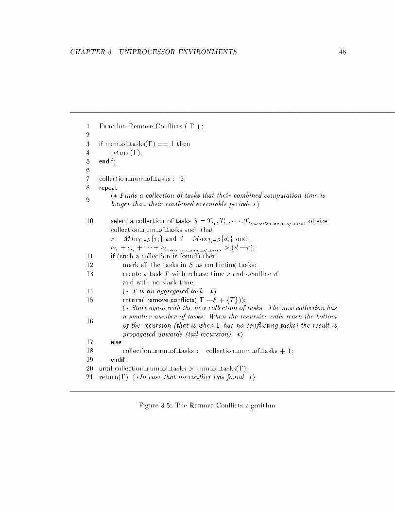
CHAPTER 3. UNIPROCESSOR ENVIRONMENTS 46
1 Function Remove Con icts ( � ) ;23 if num of tasks(�) == 1 then4 return(�);5 endif;67 collection num of tasks :=2;8 repeat
9(� Finds a collection of tasks that their combined computation time islonger than their combined executable periods �)
10 select a collection of tasks S = Ti1 ; Ti2; � � � ; Ticollection num of tasksof size
collection num of tasks such thatr = MinTi2Sfrig and d = MaxTi2Sfdig andci1 + ci2 + � � �+ cicollection num of tasks
> (d� r);11 if (such a collection is found) then12 mark all the tasks in S as con icting tasks;13 create a task T with release time r and deadline d
and with no slack time;14 (� T is an aggregated task �)15 return( remove con icts( � � S + fTg));
16
(� Start again with the new collection of tasks. The new collection hasa smaller number of tasks. When the recursive calls reach the bottomof the recursion (that is when � has no con icting tasks) the result ispropagated upwards (tail recursion). �)
17 else
18 collection num of tasks := collection num of tasks + 1;19 endif;20 until collection num of tasks > num of tasks(�);21 return(�) (�In case that no con ict was found �)
Figure 3.5: The Remove Con icts algorithm.
CHAPTER 3. UNIPROCESSOR ENVIRONMENTS 47
con icting tasks10.
Dover schedules to completion all con ict-free tasks (thus all tasks in an underloaded
system) and also obtains at least 1(1+
pk)2
times the value a clairvoyant algorithm can get
from the con icting tasks. The proof rests on the proof of the competitive guarantee given
in this chapter and can be found in appendix 3.3.
10Note that the purpose of this algorithm is to de�ne con icting and con ict free tasks. No scheduler
needs ever to execute it.
Chapter 4
Multiprocessor Environments
48
CHAPTER 4. MULTIPROCESSOR ENVIRONMENTS 49
4.1 The Lower Bound
We would �rst like to show that every on-line algorithm has a competitive multiplier of at
least k
(k�1)n(k1
n� 1) for a system with n processors and importance ratio of k. As usual in
proofs of this kind we assume that a game is played between an adversary and the on-line
scheduler.
We consider n+1 possible levels of value density 1; k1
n ; k2
n ; � � � ; kn
n = k call them levels
0; 1; � � � ; n. With each level we associate a period. A task of some value density level will
have a computation time and deadline equal to the corresponding period. Hence the value
of a task of level i equals the length of the i'th period times the i'th value density. The
length of the 0'th level's period is set to 1. We choose all other periods in such a way that
the value of an i + 1'th level task is only a small fraction of the i'th level task's value. In
fact we choose it so the i+1'th task's e�ective value density1 taken over the i'th period is
arbitrarily small (say � for some small �). A collection of tasks that has n identical tasks
for each level where all are released at the same time is called acomplete set2. Figure 4.1
shows a complete set for a system with 3 processors and value density of 8.
The adversary controls the release of tasks making decisions after observing the actions
(schedule) of the on-line algorithm so far. In the following we describe the game played by
the adversary and the on-line scheduler.
The game is played by stages the �rst one beginning at time 0. At the beginning of
each stage the adversary releases a complete set of tasks. The adversary releases tasks only
in complete sets and only in the beginning of a stage. The behavior of the on-line scheduler
dictates when the next complete set is to be released (i.e the beginning of the next stage).
Denote by tl the beginning of the l'th stage. At time tl (in particular at time 0) the on-
line algorithm has to schedule a new complete set and possibly some previously released
tasks. The number of possible scheduling decisions is vast. However since the number of
processors is smaller than the number of levels at least one level is not represented in the
on-line schedule (at time tl). Let i0 be an index of some level (to be speci�ed later) that
is not represented. Then tl+1 is set to be the end of the current i0'th level period. This
means that up to that time there will be no new task releases. We will say that the stage
starting at tl is associated with level i0. The game goes on in that manner for a big enough
1See de�nition 4.1.1.2Hence, a complete set has n(n+ 1) tasks.
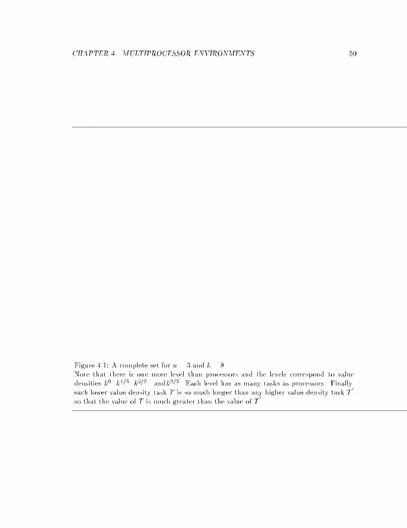
CHAPTER 4. MULTIPROCESSOR ENVIRONMENTS 50
Figure 4.1: A complete set for n = 3 and k = 8.
Note that there is one more level than processors and the levels correspond to value
densities k0 k1=3 k2=3 andk3=3. Each level has as many tasks as processors. Finally
each lower value density task T is so much longer than any higher value density task T0
so that the value of T is much greater than the value of T0
.
CHAPTER 4. MULTIPROCESSOR ENVIRONMENTS 51
number of stages (see proof of theorem 4.1.3).
Suppose that the stage starting at tl is associated with level i0 then what can the
clairvoyant scheduler do? One possibility is to execute n tasks of level i0 to completion
between tl to tl+1. In this scheme the clairvoyant scheduler schedules all the processors in
the same way no processor is ever idle and all current tasks complete immediately before
a new set is released.
The idea behind the lower bound game is that while the clairvoyant scheduler gets a
value density of ki0
n for the duration of the entire stage on all the processors. The on-line
scheduler utilizes its processors either with lower value density tasks or with higher value
density tasks that have very short duration (hence have little value). After the completion
of these short high value density tasks the associated processors will be left idle because
no more tasks are released before the end of the stage.
The question is how to choose the level associated with a given stage. In the case that
only one value density is missing from the on-line schedule then this level is the one. We
will start by proving results assuming that only one level is missing. Later we will show
that these results hold in the general case when more than one level of value density is
missing.
De�nition 4.1.1 Effective Value Density
The e�ective value density obtained by a scheduling algorithm A at the period between
time t1 and t2 is the sum of value densities scheduled during this period weighted according
to their length of execution during the period. Formally for any task T letduration(T )
denote the duration for which T was scheduled (by A) between time t1 and t2. Then the
e�ective value density of the algorithm A between t1 and t2 is:
X value density(T )� duration(T )
t2 � t1
The sum is taken over all T such that T was scheduled for execution between t1 and t2.
We will say that the the e�ective value density of a task T between t1 and t2 is its
contribution to the above sum. I.e.
value density(T )� duration(T )
t2 � t1
Lemma 4.1.1 If only one density level, i0, is missing from the on-line schedule at the
beginning of some stage, S, then the e�ective value density obtained by the clairvoyant
CHAPTER 4. MULTIPROCESSOR ENVIRONMENTS 52
scheduler during stage S is at least k
(k�1)n(k1
n � 1) times bigger than the e�ective value
density obtained by the on-line scheduler for the same period.
proof.
An easy lower bound on the value achieved by the clairvoyant algorithm is obtained by
scheduling to completion n tasks of level i0. This corresponds to an e�ective value density
of nki0
n .
During stage S the on-line scheduler did not execute any task of level i0 because no task
of that level was scheduled at the beginning of the stage and no new tasks are released
before the end of the stage. Instead it scheduled tasks of lower or higher levels. The
e�ective value density of any task of higher level is much smaller than its value density
because of its short period. In fact all such tasks have e�ective value density of at most �
during S. Hence the e�ective value density achieved by the on-line scheduler is at most
1 + k1
n + k2
n + � � �+ ki0�1
n + � + � � �+ �| {z }
n�i0 times
We are looking for the smallest possible ratio between the e�ective value densities of the
clairvoyant and the on-line scheduler. That is
min0�i0�n
nki0
n
(1 + k1
n + k2
n + � � �+ ki0�1
n + (n � i0)�)
The above term monotonically decreases when i0 increases hence the minimum is obtained
when i0 = n and its value is
nk
1 + k1
n + k2
n + � � �+ kn�1
n
=k
k � 1n(k
1
n � 1)
and the lemma is proved.
The preceding lemma dealt with the special case that only one value density level is
missing from the on-line schedule. But what will happen if more than one level is missing?
In the following we show that this cannot bene�t the on-line scheduler (for a \good" choice
of i0). Hence the lower bound holds in the general case.
Actually we look for a value density level (at time tl) that has the following single
representative property: No task of that level is currently executing and all lower levels
CHAPTER 4. MULTIPROCESSOR ENVIRONMENTS 53
have only one representative in the on-line schedule3 (recall that each level can have up to
n representatives). This level will give us the desired result.
Still it is possible that no such level exists. That is it may be that some levels lower
than the missing one have more than one representative. In that case we show that we
always can help the on-line scheduler by the following gift: we promote some tasks upwards
to higher value densities i.e. giving them an additional value density during one stage.
We choose the promotion in such a way that it leads to a situation that satis�es the above
property. Then we obtain the lower bound taking the gift into consideration. This bound
surely applies for the weakened on-line scheduler (i.e. without the gift).
Here are the details of the promotion procedure. At the beginning of the stage the
on-line scheduler executes up to n tasks. The promotion works as follows: group the tasks
currently executing according to their value density levels. Now starting from level zero
go up the levels until a level having the single representative property is found. If there is
no task at level zero then level zero has the desired property. Otherwise promote allbut
one of the tasks one level up to level one. Now we repeat this procedure for level one: if
there are no tasks at level one (taking into consideration tasks that were just promoted)
then level one satis�es the desired property. If level one is not empty then we promote all
but one of the tasks (if any) to the next level and repeat this process.
There are n + 1 value density levels but only n (or less) tasks hence this process
must terminate producing a \promoted" schedule with a level that has the the single
representative property.
Now we are ready to state and prove the version of lemma 4.1.1 for the general case
(i.e. when more than one level is missing).
Lemma 4.1.2 For any stage S, the e�ective value density obtained by the clairvoyant
scheduler during S is at least k
(k�1)n(k1
n � 1) times bigger than the e�ective value density
obtained by the on-line scheduler for the same period.
proof.
Suppose i0 is the level having the single representation property for the period in question
possibly after performing the promotion procedure.
An easy lower bound on the value achieved by the clairvoyant algorithm is obtained by
3If only one level is missing from the schedule then the single representative property is satis�ed for that
level.
CHAPTER 4. MULTIPROCESSOR ENVIRONMENTS 54
scheduling to completion n tasks of level i0. This corresponds to an e�ective value density
of nki0
n .
Suppose T1; T2; � � �Tm with value densities i1 � i2 � � � � im < i0 are the tasks that were
executing at the beginning of stage S 4. There are no more tasks releases until the end of
i0's period. Hence the ratio between the e�ective value densities is at least:
nki0
n
(ki1n + k
i2n + � � �+ k
im
n + (n�m)�)
But if we replace the value density of a task T by its promoted value density (denoted by
P (�)) then the denominator does not decrease hence the ratio does not increase.
nki0n
(ki1n + k
i2n + � � �+ k
im
n + (n�m)�)
�nk
i0n
(kP (i1)n + k
P (i2)n + � � �+ k
P (im)n + (n�m)�)
�nk
i0n
(k1n + k
2n + � � �+ k
m
n + (n�m)�)
The last equality is due to the fact that P is a one to one function from fi1; i2; � � � img onto
f1; 2; :::mg. We saw in lemma 4.1.1 above that the above ratio is not smaller than
k
k � 1n(k
1n � 1)
and the lemma is proved.
The lemma above demonstrates a ratio between the e�ective value density of any on-line
scheduler and that of the clairvoyant scheduler during every stage. For an in�nite game
this translates to a ratio between the values obtained by the algorithms during the entire
game. However we are interested in �nite games: a problem arises with the end of the
last stage. At the end of the last stage the on-line scheduler may still execute tasks from
previous stages while the clairvoyant (according to our scenario) leave all the processors
idle. The following theorem proves that after su�cient number of stages these \residual"
tasks can be ignored.
4It is possible that some of these tasks were released in previous stages.
CHAPTER 4. MULTIPROCESSOR ENVIRONMENTS 55
Theorem 4.1.3 For a system with n processors and maximal value density of k, there is
no on-line scheduling algorithm with competitive multiplier smaller than k
(k�1)n(k1
n � 1).
proof.
Fix an on-line scheduling algorithm. Recall that tl the beginning of the l'th stage denote
by V (tl) the value obtained by the on-line scheduler until time tl. The ratio between the
e�ective value densities as appears in lemma 4.1.2 becomes a lower bound on the ratio
between values because the clairvoyant scheduler never abandons a task that started its
execution while the on-line algorithm might. Hence lemma 4.1.2 shows that the value
obtained by the clairvoyant algorithm is at least k
(k�1)n(k1
n � 1)V (tl).
Note that tl tends to in�nity as l goes to in�nity. If V (tl) does not tend to in�nity as
l goes to in�nity then the competitive multiplier of the on-line algorithm is not bounded
(because the clairvoyant algorithm gets a value of at least ntl !1). Hence we can assume
that V (tl) tends to in�nity. For arbitrarily small � > 0 there is a big enough l0 such that
V (tl0) �1
�kn) kn � �V (tl0)
Suppose the game ends at tl0 (i.e. no more task releases). The total value obtained by the
on-line scheduler is not greater than V (tl0) + kn (because all the tasks not yet completed
have length at most 1 and value density at most k). The clairvoyant scheduler gets a value
of at least k
(k�1)n(k1
n � 1)V (tl0).
Hence
value obtained by the clairvoyant scheduler
value obtained by the on-line scheduler
�
k
(k�1)n(k1
n � 1)V (tl0)
V (tl0) + kn
�
k
(k�1)n(k1
n � 1)V (tl0)
V (tl0) + �V (tl0)
�
k
(k�1)n(k1
n � 1)
1 + �
This holds for every positive � hence the Theorem is proved.
Corollary 4.1.4 As the number of processors n tends to in�nity, no on-line algorithm
can have a competitive multiplier smaller than ln k (natural logarithm).
CHAPTER 4. MULTIPROCESSOR ENVIRONMENTS 56
Remark 4.1.2 For n = 1 the lower bound is k which is not as good as the already known
tight lower bound of (1 +pk)2 (chapter 3). For k = 1 a di�erent treatment is needed.
In the next section we introduce our competitive scheduling algorithm for multiproces-
sor environments.
4.2 Algorithmic Guarantees
Having proved the lower bound on the best possible competitive multiplier we would like
to devise an on-line scheduler that achieves this bound. In the following we describe an
algorithm that does so (up to a small multiplicative factor) in many cases.
We break the processors into bands (of 2 processors each) and one central pool. The
main idea of the algorithm is to assign a task upon its release to the band corresponding to
its value density. Tasks that are assigned to a band are guaranteed to complete and can all
complete on a single processor. This means that they constitute a uniprocessor underloaded
system and can be scheduled according to the earliest-deadline-�rst algorithm [7]. Suppose
the new task cannot be added to the band that corresponds to its value density (because
it will cause overload at that band). Then the scheduler will determine whether the new
task can be scheduled on the next band below (i.e a band corresponding to lower value
density). If the band below cannot accept the new task the task will continue to cascade
downwards. If a task cascades to the lowest band but still cannot be scheduled there it
can go into the central pool.
If a newly released task is accepted by one of the bands or by the central pool it is
guaranteed to complete before its deadline (these tasks are called \privileged"). If it is
not it awaits its LST (Latest Start Time)5 at which time it tries again to be scheduled
(details to follow).
Throughout this section we assume a system with 2n processors. We break the pro-
cessors into two disjoint groups: 2 processors will constitute a \band structure" and the
other 2! processors will constitute a \central pool" as described below (n = + !; and
n > ! � 0).
5Recall the de�nition of LST (section 3.1): LST = (deadline - remaining computation time). If a taskis not scheduled at its LST, it will not complete.
CHAPTER 4. MULTIPROCESSOR ENVIRONMENTS 57
We consider intervals6 (levels) of value density [1::k1
); [k1
::k2
); � � � ; [k �1 ::k] call
these levels 1; � � � ; respectively. The i'th band is said to be \lower" than the i + 1'st
band.
Suppose the entire set of tasks to be scheduled is �. We partition this set according
to the value density of the tasks: � = �1 [ �2 � � � [ � where �i contains all tasks with
value density in the range [ki�1
; ki
). We allocate 2 processors (a band) for each of the
value density levels. In addition the remaining 2! processors are allocated as a central
pool that will be used by tasks of all levels.
The algorithm has three major components:
1. Upon task release assign a task to a band (possibly after cascading).
2. At LST (of a non-privileged task) decide whether and where a task should be sched-
uled or maybe abandoned.
3. The method used in scheduling each band (and the central pool).
Di�erent choices for these three components would create di�erent variants of the algo-
rithm. In this paper we describe one speci�c variant that we call the MOCA Algorithm.
In this variant the central pool is also broken into bands of two processors each7. The
MOCA Algorithm schedules according to the following rules:
� At each moment every band has one of its processors designated as the Safe Processor
(SP) and the other as the Risky Processor (RP). Each band has its own queue called
Q privileged the tasks inQ privileged are guaranteed to complete. In addition to
the local Q privileged queues there is one global queue called Q waiting . This queue
includes all the ready tasks that are not privileged.
� When a new task T is released it is assigned to a band as follows:
6All but the last interval is half open half closed. The last level corresponds to the closed interval
[k
�1 ; k].7The bands of the central pool are ordered so that a task that reaches the pool start with the �rst band
in the pool and if not accepted it cascades to the second band and onwards. If the task is not accepted bythe last band in the pool it awaits its LST.
CHAPTER 4. MULTIPROCESSOR ENVIRONMENTS 58
1. It is added to the Q privileged of its own band if this does not create overload
(i.e all tasks including the new task can complete on SP). Otherwise T cascades
downward as described above.
2. If T was not accepted by any band (including all the bands in the central pool)
it enters Q waiting where it waits until its LST occurs.
So at release time only the SPs are examined. A task might not be scheduled even
if an RP is idle8.
� A task T that reached its LST is assigned to a processor as follows:
1. If there is any idle RP among all the lower level bands (including T 's own level)
then schedule T on one of these processors9.
2. If there is no idle RP among lower level bands we might abandon a task exe-
cuting on one of these RPs in order to schedule T depending on the following
rule:
Let T � be the task with earliest deadline among all the tasks executing on these
RPs.
If T has a later deadline than T� then abandon T
� and schedule T in its place;
otherwise abandonT 10.
� If at task completion event SP of a band becomes idle then the two processors
should switch roles; the safe-processor becomes the risky-processor and vice versa11.
This does not require task migration.
Figure 4.2 is a schematic description of the MOCA Algorithm. The bands structure as
described above prioritize high value density tasks over low value density tasks. Higher
value density tasks start their cascading at a higher point and cascading is possible in only
one direction - downwards12. However an algorithm that uses the \pure" bands structure
8Using idle RPs and scheduling tasks of Q waiting before they reach their LST is a heuristic that canimprove the average case behavior of the scheduler.
9Heuristics can be used to choose the processor in case more than one RPis idle.10If T is to be abandoned while there is an idle processor (above T 's own band), scheduling T on an idle
processor (with or without guaranteeing its completion) can only improve the average case behavior of thescheduler.
11The current task on SP (that was RP) becomes privileged.12Hence, higher value density tasks have more bands that can possibly accommodate them.
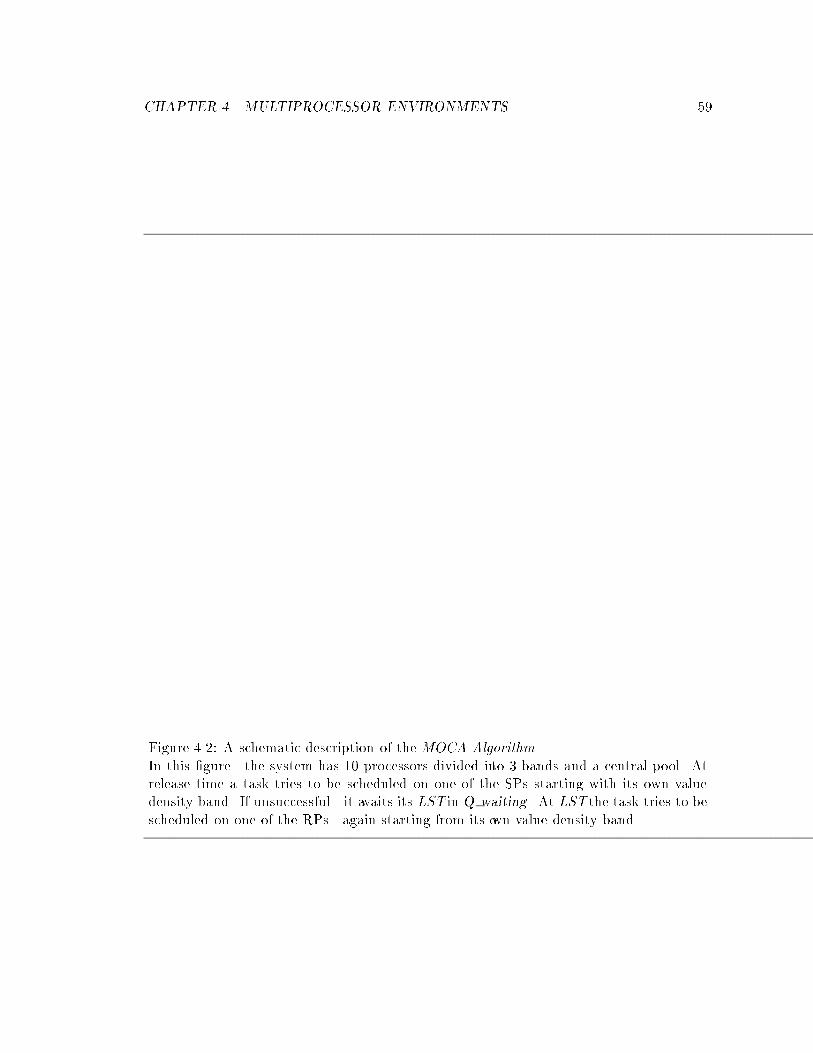
CHAPTER 4. MULTIPROCESSOR ENVIRONMENTS 59
Figure 4.2: A schematic description of the MOCA Algorithm.
In this �gure the system has 10 processors divided into 3 bands and a central pool. At
release time a task tries to be scheduled on one of the SPs starting with its own value
density band. If unsuccessful it awaits its LST in Q waiting . At LST the task tries to be
scheduled on one of the RPs again starting from its own value density band.
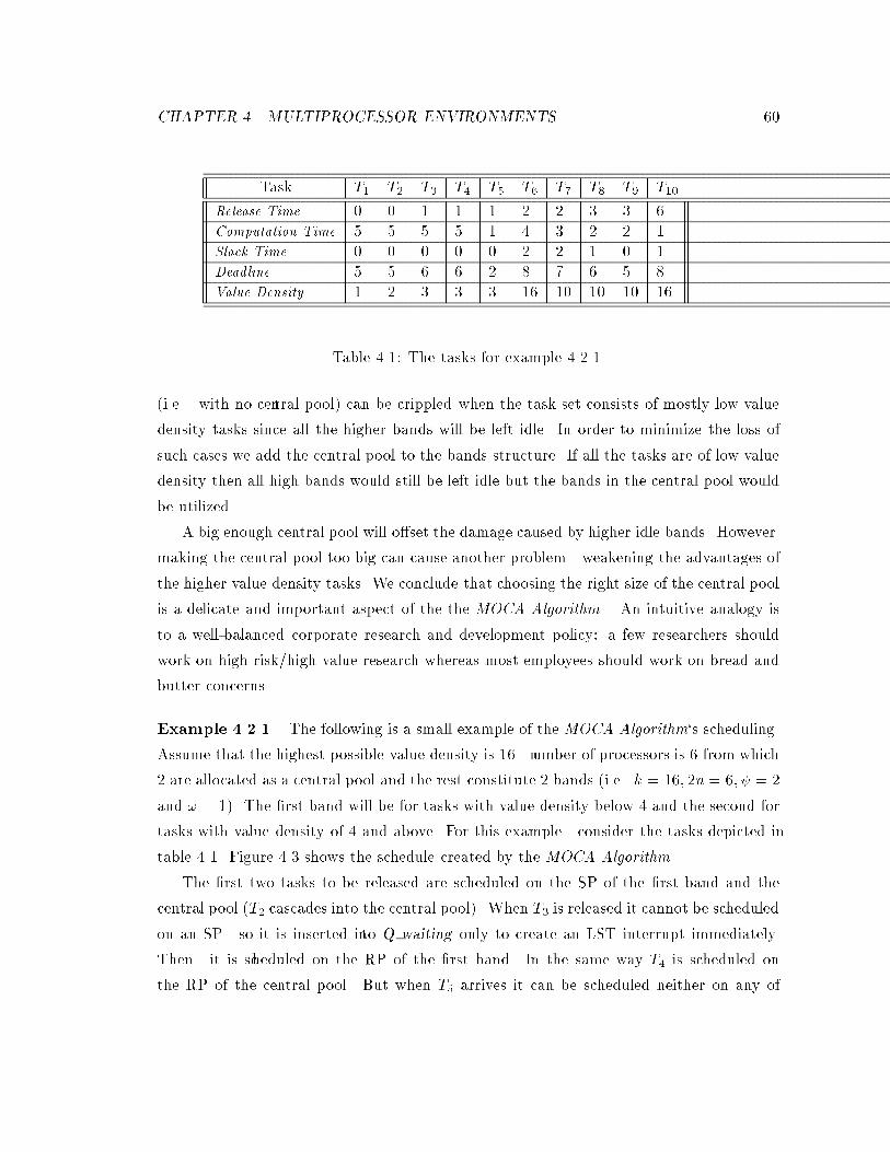
CHAPTER 4. MULTIPROCESSOR ENVIRONMENTS 60
Task T1 T2 T3 T4 T5 T6 T7 T8 T9 T10
Release Time 0 0 1 1 1 2 2 3 3 6
Computation Time 5 5 5 5 1 4 3 2 2 1
Slack Time 0 0 0 0 0 2 2 1 0 1
Deadline 5 5 6 6 2 8 7 6 5 8
Value Density 1 2 3 3 3 16 10 10 10 16
Table 4.1: The tasks for example 4.2.1.
(i.e. with no central pool) can be crippled when the task set consists of mostly low value
density tasks since all the higher bands will be left idle. In order to minimize the loss of
such cases we add the central pool to the bands structure. If all the tasks are of low value
density then all high bands would still be left idle but the bands in the central pool would
be utilized.
A big enough central pool will o�set the damage caused by higher idle bands. However
making the central pool too big can cause another problem|weakening the advantages of
the higher value density tasks. We conclude that choosing the right size of the central pool
is a delicate and important aspect of the the MOCA Algorithm. An intuitive analogy is
to a well-balanced corporate research and development policy: a few researchers should
work on high risk/high value research whereas most employees should work on bread and
butter concerns.
Example 4.2.1 The following is a small example of the MOCA Algorithm`s scheduling.
Assume that the highest possible value density is 16 number of processors is 6 from which
2 are allocated as a central pool and the rest constitute 2 bands (i.e. k = 16; 2n = 6; = 2
and ! = 1). The �rst band will be for tasks with value density below 4 and the second for
tasks with value density of 4 and above. For this example consider the tasks depicted in
table 4.1. Figure 4.3 shows the schedule created by the MOCA Algorithm.
The �rst two tasks to be released are scheduled on the SP of the �rst band and the
central pool (T2 cascades into the central pool). When T3 is released it cannot be scheduled
on an SP so it is inserted into Q waiting only to create an LST interrupt immediately.
Then it is scheduled on the RP of the �rst band. In the same way T4 is scheduled on
the RP of the central pool. But when T5 arrives it can be scheduled neither on any of
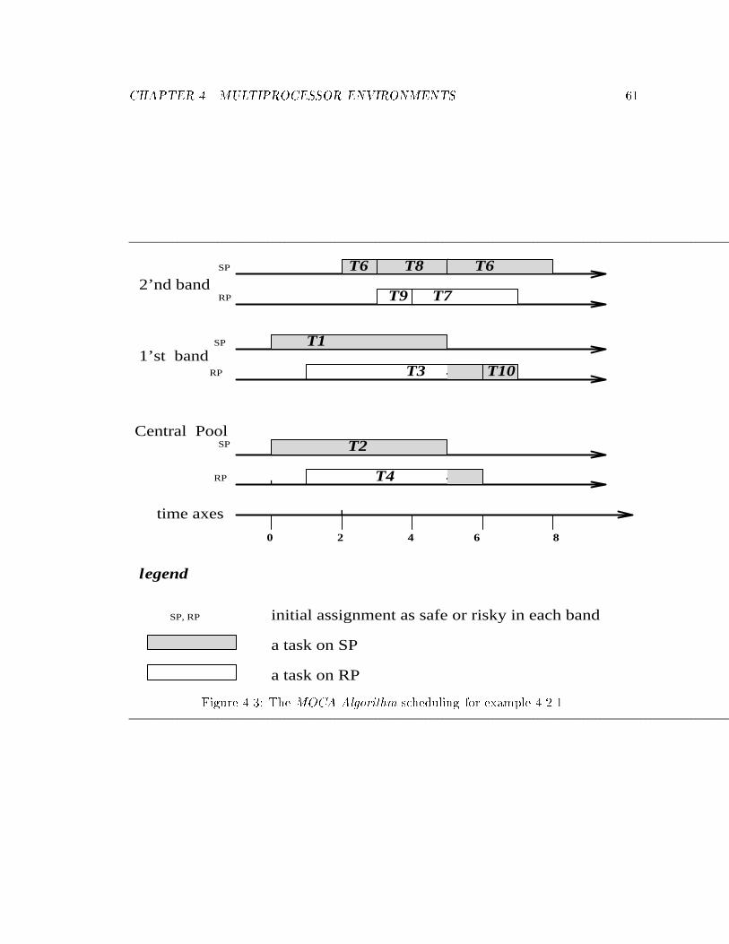
CHAPTER 4. MULTIPROCESSOR ENVIRONMENTS 61
T10
SP
RP2’nd band
Central Pool
SP
RP
RP
0 2 4
T6 T8
T4
T9 T7
T1
6 8
T6
T3
T2
a task on RP
a task on SP
legend
time axes
SP
SP, RP initial assignment as safe or risky in each band
1’st band
Figure 4.3: The MOCA Algorithm scheduling for example 4.2.1.
CHAPTER 4. MULTIPROCESSOR ENVIRONMENTS 62
the SPs nor on any of the RPs hence is abandoned (in the LST routine). Note thatT5 is
abandoned even though the second band is idle (a task can cascade only downwards).
All the remaining tasks have value density high enough to be scheduled on the second
band. T6 is scheduled on the SP. T7 cannot be scheduled on any of the SPs and it enters
Q waiting (with LST at 4). T8 can be added to the SP of the second band preempting T6
(which has a latter deadline). T9 cannot be scheduled on any of the SPs; it reaches its LST
and is scheduled on the RP of the second band but at time 4 it is abandoned in favor of
T7 which arrived to its LST and has a later deadline.
At time 5 the SP of the �rst band becomes idle which creates a switch of roles between
the SP and RP of that band. Later at time 6 T10 is released; it cannot be scheduled on
its own band's SP but after cascading it is scheduled on the (new) SP of the �rst band.
All in all theMOCA Algorithm completed all the tasks but T5 and T9. A clairvoyant
scheduler could schedule all the tasks (T5 can be scheduled on the idle SP and T9 can be
scheduled before its LST on the same processor).
4.3 The Algorithm's Competitive Multiplier
In this section we would like to study the behavior of theMOCA Algorithm and to compute
its competitive multiplier. The �nal result is stated in theorem 4.3.3. Before we start we
must introduce the lost value lemma as well as some notation and de�nitions.
Let A be an on-line scheduler and � a set of tasks to be scheduled. We can partition
the tasks of � according to the behavior of A
1. Tasks that never completed (F ) the \lost" ones.
2. Tasks that completed successfully (S)
� = F [ S
Denote by V (�) and C(�) the value achieved by A and the clairvoyant scheduler from the
tasks of � respectively.
Lemma 4.3.1 The Lost Value Lemma
CHAPTER 4. MULTIPROCESSOR ENVIRONMENTS 63
If for some constant c and every set of tasks �,
C(F ) � cV (�)
Then,
C(�) � (c+ 1)V (�)
proof.
C(�) = C(F [ S) � C(F ) + C(S)
= C(F ) + V (S) = C(F ) + V (�)
� (c+ 1)V (�)
De�nition 4.3.1
� Productive Band: A band is said to be productive at time t if at that time its
SP is not idle.
Recall that tasks that start executing on SP are never abandoned. This mean that
whenever SP is not idle it \generates" value (i.e. productive).
� Cumulative Value Density (CVD): Suppose some schedule is chosen thecu-
mulative value density at time t is the sum of the value densities of all tasks executing
at time t 13 .
Recall that � is the entire set of tasks to be scheduled. We partition the tasks of �
according to the behavior of the MOCA Algorithm: tasks that never completed (F ) and
tasks that completed successfully (S). Denote by V (�) the value achieved by the MOCA
Algorithm.
We would like to show that for any task that was abandoned by the MOCA Algorithm
there are other tasks with \enough value" that were completed. This will show that
13For example, for a system with 2n processors, if all processors are idle at time t then CV D(t) = 0. Ifhalf of the processors (i.e, n) execute tasks with unit value density and the others execute tasks of valuedensity k then the cumulative value density is n+ kn. In no case can CV D(t) be bigger than 2nk.
CHAPTER 4. MULTIPROCESSOR ENVIRONMENTS 64
C(F ) � �C(�) (for some constant �). Using the Lost Value Lemma (4.3.1) we will get a
competitive multiplier of � + 1.
First we note that only tasks of level i or higher can be scheduled on band i. Suppose
a task T was abandoned by the MOCA Algorithm we will show that this implies that all
the bands corresponding to the value density of T or lower were productive during the
entire executable period14 of T . If a band was productive during the executable period of
T then theMOCA Algorithm gains a value of at least the band's value density times the
length of the period. In this way we get a lower bound on the value gained by the MOCA
Algorithm (i.e. the \enough value" mentioned above).
The following technical lemma is used in item 2 below.
Lemma 4.3.2 If at time t a task with deadline d is executing on RP of a band (i.e this
task was scheduled by an LST interrupt) then that band will be productive between t and
d.
proof.
If SP does not become idle before time d then by de�nition the band is productive between
t and d. Otherwise suppose SP becomes idle at times t < s < d then there must be a
task executing on RP at time s (because a task on RP can be abandoned only in favor of
another task with a later deadline and no slack time). So at times RP becomes SP and
it would not become idle before time d because the deadline of the current task is at least
d (and it has no slack time).
Here are a few things to notice about the MOCA Algorithm:
1. At any band i only tasks of level i or higher can be executed.
2. If a task T of level i is abandoned then band i and all lower bands (including the
central pool) are productive during the entire executable period of T .
proof.
Let T be T (r; c; d)15. Upon T 's release it was not accepted by any of the levels on or
below i. This means that for each of these bands the tasks currently in (the local)
14Recall the de�nition of executable period (2.0.1).15I.e., released at time r with deadline d and computation time c.
CHAPTER 4. MULTIPROCESSOR ENVIRONMENTS 65
Q privileged will execute at least until d� c (otherwise T could become privileged).
This proved that all bands are productive between r and d� c.
However d� c is the LST of T . At its LST T would not be scheduled only if every
band (on or below the i'th) has a task currently executing on its RP with deadline
after d. This means that all bands are productive between d�c and d (lemma 4.3.2).
Combining the two gives the desired result.
3. Once a task starts to execute on some processor it will never migrate to another
processor.
At any given time t consider all the tasks ofF for which t is in their executable period.
Let high(t) be the value density level corresponding to the task with the highest value
density among all these tasks.
Suppose the clairvoyant scheduler has to schedule only the tasks of F and suppose
it had chosen some optimal schedule for these tasks. At time t the best the clairvoyant
scheduler can hope for (looking only at time t) is to have all 2n processors executing tasks
of level high(t) i.e with value density not greater than k
high(t)
. We conclude that the
cumulative value density of the clairvoyant schedule at time t is bounded by 2nkhigh(t)
.
The facts that a task of level high(t) was abandoned and that t is in its executable
interval imply that at time t all bands up to (and including)high(t) were productive.
This means that the on-line scheduler has a cumulative value density of at least16:
! + 1 + k1
+ k2
+ � � �+ k
high(t)�1
= ! +(k
high(t)
� 1)
(k1
� 1)
This leads to the following theorem.
Theorem 4.3.3 For a system with 2n processors and maximal value density of k > 1 the
MOCA Algorithm has a competitive multiplier of at most
1 + 2n min(0� �n;n=!+ )
8>>>>>><>>>>>>:
max1�i�
ki
! + (ki
�1)
(k1
�1)
9>>>>>>=>>>>>>;
(4.1)
16For the case k = 1, the uniform value density case, see remark 4.3.2 below.
CHAPTER 4. MULTIPROCESSOR ENVIRONMENTS 66
proof.
The discussion above demonstrated that
C(F )
V (�)� max
1�i�
2nki
! + (k
i
�1)
(k
1
�1)
= 2n max1�i�
k
i
! + (k
i
�1)
(k
1
�1)
(4.2)
Since this is true for any setting of (provided that n = ! + ) hence we get
C(F )
V (�)� 2n min
(0� �n;n=!+ )
8>>>>>><>>>>>>:
max1�i�
k
i
! + (k
i
�1)
(k
1
�1)
9>>>>>>=>>>>>>;
Using the Lost Value lemma we get the desired result.
Remark 4.3.2
� Note that the MOCA Algorithm does not use migration hence the previous result
holds both whether migration is allowed or not.
� When k = 1 there is no need for the bands structure hence the central pool consists
of all the processors (in our notation ! = n�1 and = 1). This leads to a competitive
multiplier of 2+1 (when some tasks may have slack time). For n = 2 this corresponds
to our results for two processor systems (in appendix D).
� When the number of processor is odd a similar result can be obtained. For a system
with 2n+ 1 processors create bands and pool from the �rst 2n processors. The left
over processor can be used for example as a second SP for one of the bands. This
leads to a bound of:
1 + (2n+ 1) min(0� �n;n=!+ )
8>>>>>><>>>>>>:
max1�i�
k
i
! + (k
i
�1)
(k
1
�1)
9>>>>>>=>>>>>>;
However this result does not specialize to a uniprocessor system because at least two
processors are needed to create a band.
CHAPTER 4. MULTIPROCESSOR ENVIRONMENTS 67
4.3.1 Setting
We will estimate the complex expression for the upper bound on the competitive multiplier
given by theorem 4.3.3 by setting17 18 = nlnk
ln k+1. (hence ! = n
1ln k+1
= ln k
) The bound
in (4.2) above becomes:
2n max1�i�
k
i
ln k
+ k
i
�1
k
1
�1
= 2n(k1
� 1) max
1�i�
k
i
ln k
(k1
� 1) + (k
i
� 1)
The left hand side is obtained by multiplying both numerator and denominator by (k1
�1).
The maximum19 denoted by the equation above is attained at i = and the upper bound
(equation 4.2) is:
2n(k1
� 1)
k
ln k
(k1
� 1) + (k � 1)
< 2n(k1
� 1)
k
1 + (k� 1)= 2n(k
1
� 1) (4.3)
We have just proved the following lemma:
Lemma 4.3.4 The MOCA Algorithm has a competitive multiplier of at most
1 + 2n(k1
� 1) (4.4)
where = nln k
ln k+1
(recall that the lower bound is bigger than 2n(k1
2n� 1))
Recall that (k1
� 1) tends to ln k as approaches in�nity. Hence when the number
of processors tends to in�nity equation (4.4) above tends to
1 + 2 lim !1
ln k + 1
ln k(k
1
� 1) = 1+ 2
ln k + 1
ln kln k = 2 ln k + 3 (4.5)
17ln is the natural logarithm18Numerical experiments have shown that this setting of is a close approximation to the optimal
setting.19De�ne fa(x) to be x
a+(x�1). When a > 1, this function is monotone increasing with x (x � 0). Let a
be ln k (k
1
� 1). Then a is bigger than 1, because k1
�1
ln k is a monotone decreasing function of tendingto 1 when goes to in�nity.
CHAPTER 4. MULTIPROCESSOR ENVIRONMENTS 68
Corollary 4.3.5 For given n and k, the ratio between the lower bound and the algorithmic
guarantee is at most
1 + 2n(k1
� 1)
k
k�12n(k
1
2n� 1)
; where = nln k
ln k + 1(4.6)
When k is held �xed and n tends to in�nity this ratio tends to k�1
k
�2 + 3
ln k
�. Which, is
less then 3:2 for all k > 1 and tends 2 as k tends to in�nity.
proof.
Recall our lower bound of 2n k
k�1(k
1
2n� 1). This bound tends to k
k�1ln k when n tends to
in�nity. The limit of the ratio is the ratio of the limits which is:
2 ln k + 3k
k�1ln k
=k � 1
k
�2 +
3
ln k
�(4.7)
Which gives the desired result.
Figure 4.4 gives a graphical representation of the above result.
Remark 4.3.3 In the discussion above we have chosen to ignore the fact that ! and
must be integers. We can take care of that by setting as the nearest integer to n lnklnk+1
4.3.2 Distributed vs. Centralized Scheduler
We discuss here architectures with large number of processors. Hence it is necessary to
see which portions of the scheduler are centralized and which are distributed. The MOCA
Algorithm uses a central scheduler in order to assign a task to a band (at task release time
and LST). This means that the centralized scheduler has all the information regarding
tasks assigned to each band and their parameters20. Once a task is assigned to a band it
is left in the hands of the local scheduler (which basically employs earliest-deadline-�rst).
It is desirable for reasons of fault-tolerant and e�ciency [39] to distribute the func-
tionality of the centralized scheduler among the processors. This is an interesting and
important extension to the work presented here.
20Since all the tasks go through the central scheduler this is not di�cult to do.
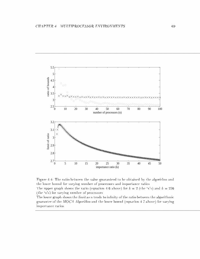
CHAPTER 4. MULTIPROCESSOR ENVIRONMENTS 69
0 5 10 15 20 25 30 35 40 45 502.7
2.8
2.9
3
3.1
3.2
importance ratio (k)
lim
it o
f ra
tio
0 10 20 30 40 50 60 70 80 90 1002.5
3
3.5
4
4.5
5
5.5
number of processors (n)
rati
o o
f b
ou
nd
s
Figure 4.4: The ratio between the value guaranteed to be obtained by the algorithm andthe lower bound for varying number of processors and importance ratios.The upper graph shows the ratio (equation 4.6 above) for k = 2 (the `x's) and k = 256(the `o's) for varying number of processors.The lower graph shows the limit as n tends to in�nity of the ratio between the algorithmicguarantee of the MOCA Algorithm and the lower bound (equation 4.7 above) for varyingimportance ratios.
CHAPTER 4. MULTIPROCESSOR ENVIRONMENTS 70
4.3.3 The Scheduling Overhead
In the previous sections we analyzed the performance of our algorithm in the sense of
their competitive multipliers. In this section we study the cost of executing the scheduling
algorithm itself.
What is the cost of testing whether a newly arriving task can be added to Q privileged
containing N tasks with out causing overload? This can be done in O(logN) operations
using a 2-3 tree that holds slack times with sums of the slack times from left siblings held
in interior nodes. If the task is to be added to Q privileged the updating of the 2-3 trees
involved takes also O(logN) time.
Let M be a bound on the the total number of ready tasks at any given moment in
Q waiting and any of the local queues. When a task is released it may have to be checked
against all bands (suppose the task cascades from the highest band all the way to the
lowest) with a total cost of O(n logM).
A task in Q waiting awaits its LST. Hence Q waiting is a 2-3 tree organized according
to Latest Start Time. Inserting and removing a task from this queue costs O(logM)
operations.
A task during its lifetime causes exactly one task release event and at most one LST
interrupt. Hence the scheduling overhead per task is O(nlogM).

Chapter 5
Conclusions
71
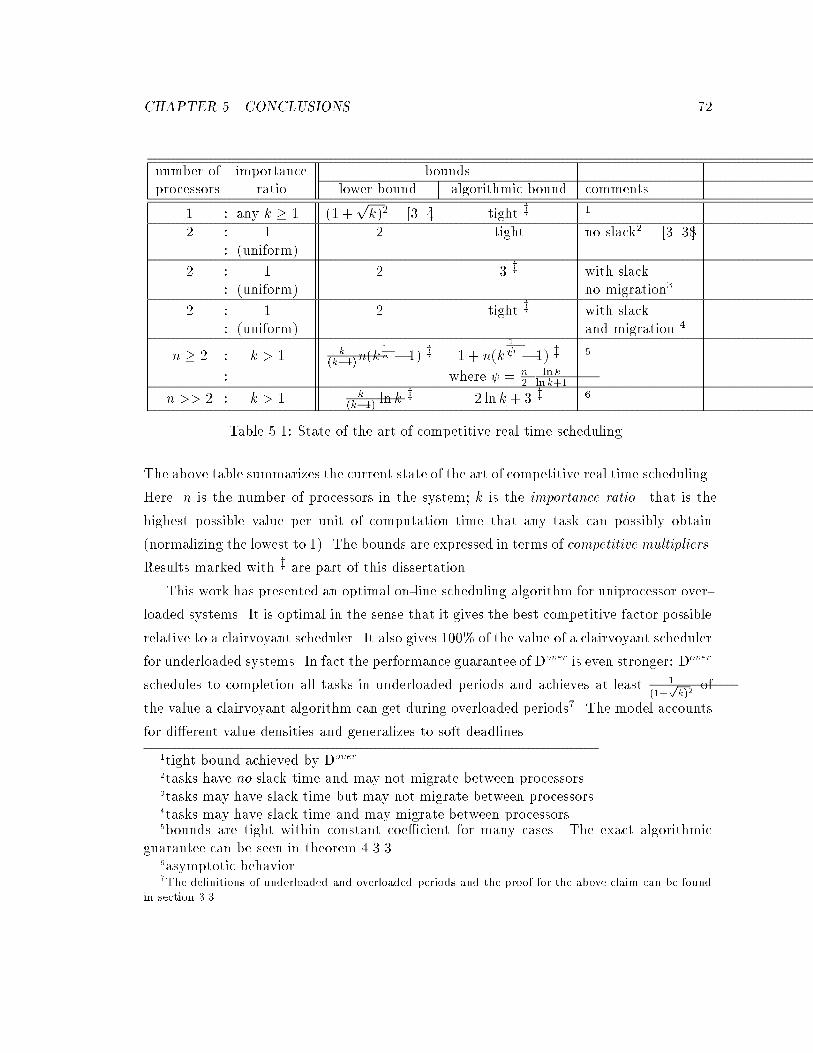
CHAPTER 5. CONCLUSIONS 72
number of importance boundsprocessors ratio lower bound algorithmic bound comments
1 : any k � 1 (1 +pk)2 [3 4] tight z 1
2 : 1 2 tight no slack2 [3 38]: (uniform)
2 : 1 2 3 z with slack: (uniform) no migration3
2 : 1 2 tight z with slack: (uniform) and migration 4
n � 2 : k > 1 k
(k�1)n(k1
n � 1) z 1 + n(k1
� 1) z 5
: where = n
2lnk
lnk+1
n >> 2 : k > 1 k
(k�1) ln kz 2 ln k + 3 z 6
Table 5.1: State of the art of competitive real time scheduling.
The above table summarizes the current state of the art of competitive real time scheduling.
Here n is the number of processors in the system; k is the importance ratio that is the
highest possible value per unit of computation time that any task can possibly obtain
(normalizing the lowest to 1). The bounds are expressed in terms of competitive multipliers.
Results marked with z are part of this dissertation.This work has presented an optimal on-line scheduling algorithm for uniprocessor over-
loaded systems. It is optimal in the sense that it gives the best competitive factor possible
relative to a clairvoyant scheduler. It also gives 100% of the value of a clairvoyant scheduler
for underloaded systems. In fact the performance guarantee of Dover is even stronger: Dover
schedules to completion all tasks in underloaded periods and achieves at least 1(1+
pk)2
of
the value a clairvoyant algorithm can get during overloaded periods7. The model accounts
for di�erent value densities and generalizes to soft deadlines.
1tight bound achieved by Dover .2tasks have no slack time and may not migrate between processors.3tasks may have slack time but may not migrate between processors.4tasks may have slack time and may migrate between processors.5bounds are tight within constant coe�cient for many cases. The exact algorithmic
guarantee can be seen in theorem 4.3.3.6asymptotic behavior.7The de�nitions of underloaded and overloaded periods and the proof for the above claim can be found
in section 3.3.
CHAPTER 5. CONCLUSIONS 73
For multiprocessor environments a gap remains between the guarantees achieved by
the MOCA Algorithm and the lower bounds we have proved. The algorithmic guarantee
is within a small multiplicative factor from the lower bound for large enough n and k
(�gure 4.4 and �gure 5.1 show that the asymptotic behavior is attained even for small
values of n). When the importance ratio of a system (i.e. k) is close to 1 a di�erent
treatment is needed. Some work in this direction has been done by Bar-Noy et. al. [2].
It is possible that a better choice of will lead to a better exact expression of the
algorithmic guarantee for our algorithm. But it seems that asymptotically we cannot
do better without changing our algorithmic techniques. The reason is that our basic
block the scheduling algorithm for a 2-processor band concentrates its e�orts on one
processor at a time (SP); the other processor RP is essentially left idle. Hence the
MOCA Algorithm automatically loses a factor of 2 compared to a clairvoyant scheduling
algorithm that utilizes all the processors concurrently. Of course one can suggest heuristics
that will use a processor whenever possible8 the true challenge is to show that such a
heuristic achieves a better worst case performance guarantee. Another way to improve the
algorithmic guarantee will be to come up with a better algorithm for an m-processor band
(for some m � 2).
Our adversary arguments and algorithms o�er two useful insights:
1. A parallel on-line scheduling algorithm achieves a competitive guarantee by allocat-
ing some processing resources according to tasks' value density. This is a qualitative
di�erence from our uniprocessor scheduling algorithm Dover which made its decisions
based on total value only. Moreover high value density tasks in the MOCA Algo-
rithm have priority over lower value density tasks in the sense that they have more
processors on which they can be scheduled due to the cascading.
2. The lower bound on the best possible competitive multiplier (as measured by our
adversary arguments) converges to k
k�1ln k as the number of processors approaches
in�nity. Our current algorithm gives a guarantee that converges to 2 ln k + 3 as
the number of processors approaches in�nity. The ratio between the algorithmic
guarantee and the lower bound is less then 3:2 for all k > 1 and a large enough n.
8Heuristic improvements can be obtained for example scheduling tasks on the Risky Processor before
tasks arrive at their latest start times.
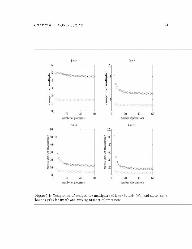
CHAPTER 5. CONCLUSIONS 74
0 20 40 600
1
2
3
4
5
6
number of processors
com
peti
tive m
ult
ipli
er
k = 2
0 20 40 600
5
10
15
20
number of processors
com
peti
tive m
ult
ipli
er
k = 8
0 20 40 600
10
20
30
40
50
60
number of processors
com
peti
tive m
ult
ipli
er
k = 64
0 20 40 600
20
40
60
80
100
120
number of processors
com
peti
tive m
ult
ipli
er
k = 256
Figure 5.1: Comparison of competitive multipliers of lower bounds (o's) and algorithmicbounds (x's) for �x k's and varying number of processors.
CHAPTER 5. CONCLUSIONS 75
This shows that the current algorithms are tight for large numbers of processors
but that work remains to be done for small numbers of processors (see �gures 4.4
and 5.1).
This work leaves many problems open. Here is a small sample.
� We assume that k is given and known in advance. It is interesting to know if this
assumption can be relaxed. Recently in an unpublished result Schieber [32] devised
a variant of Dover that gives the optimal guarantee even when k is not known in
advance. Can the same be done for multiprocessor environments?
� What guarantees can be given when tasks are not independent e.g. for systems with
locks or precedence constraints? What if some characteristics of the task set are
known a priori (e.g. periodic tasks)?
� What guarantees can be given when not all tasks can be scheduled on all processors?
What if not all processors have the same speed?
� What guarantees can be given when a penalty (i.e. a negative value) is incurred for
every task that does not complete.
� In practice real-time systems have some periodic critical tasks and other less critical
tasks which may be aperiodic. A typical solution (as taken in the Spring Kernel
for example [37]) is to devote certain intervals to the critical tasks and to allow the
less critical tasks to run during the rest of the time. Dover gives its usual guarantee
with respect to the less critical tasks in this situation (the accounting is a little more
di�cult since useful time has \holes" in it corresponding to subintervals allocated to
critical tasks). A much more subtle question is what is a good competitive algorithm
that can take advantage of the cases when a given critical task executes in less time
than is allocated for it. We suspect the competitive guarantee may be worse since
the clairvoyant algorithm might then execute a task that Dover had prematurely
abandoned.
� An important issue is how to account for migration overhead in multiprocessor envi-
ronments. For example we modeled distributed memory architectures by forbidding
migration but that is clearly too strong a restriction.
CHAPTER 5. CONCLUSIONS 76
Permitting migration but at a cost would have been much more reasonable.
� There are many other open issues that must be addressed for overloaded systems in
a fault-tolerant context. An important issue is how to reallocate processors when
a failure occurs. The MOCA Algorithm is described as a multiprocessor algorithm
with a static number of processors. Fault tolerance issues can be addressed by the
following techniques:
First one can keep some processors in reserve and introduce them as other ones fail.
While in reserve the processors can be used as a secondary pool for tasks that were
not accepted by the primary structure of bands and pool. Another way to utilize
additional reserve processors is to add a third processor to a two-processor band.
The third processor can be a mirror processor for the safe processor waiting to take
over in case that one of the band's processor fails.
Second as processors fail one can statically reset the algorithm to have a di�erent
number of bands and/or pool of shared processors. Combinations of these techniques
and additional heuristics may give rise to promising algorithms.
Bibliography
[1] N. Audsley and A. Burns. Real time system scheduling. Computer Science Depart-
ment Technical Report No. YCS134 York University UK Jan. 1990.
[2] A. Bar-Noy Y. Mansour and B. Schieber. private communication. I.B.M T.J. Wat-
son Research Center Yorktown Heights NY 1992.
[3] S. Baruah G. Koren D. Mao B. Mishra A. Raghunathan L. Rosier D. Shasha
and F. Wang. On the competitiveness of on-line task real-time task scheduling. The
Journal of Real-Time Systems 4(2):124{144 1992. Conference version appeared in
Proceedings of the 12th Real-Time Systems Symposium pages 106-115 San Antonio
Texas Dec. 1991.
[4] S. Baruah G. Koren B. Mishra A. Raghunathan L. Rosier and D. Shasha. On-line
scheduling in the presence of overload. In Proceedings of the 32nd Annual Symposium
on the Foundations of Computer Science pages 101{110 San Juan Puerto Rico Oct.
1991. IEEE.
[5] S.-C. Cheng J. A. Stankovic and K. Ramamritham. Scheduling algorithms for hard
real-time systems: A brief survey. In J. A. Stankovic and K. Ramamritham editors
Hard Real-Time Systems: Tutorial pages 150{173. IEEE 1988.
[6] H. Chetto M. Silly and T. Bouchentouf. Dynamic scheduling of real-time tasks under
precedence constraints. The Journal of Real-Time Systems 1:181{194 1990.
[7] M. L. Dertouzos. Control robotics: the procedural control of physical processes. In
Proceedings IFIF Congress pages 807{813 1974.
77
BIBLIOGRAPHY 78
[8] M. L. Dertouzos and A. K.-L. Mok. Multiprocessor on-line scheduling of hard-real-
time tasks. IEEE Transactions on Software Engineering 15(12):1497{1506 Dec. 1989.
[9] S. K. Dhall and C. L. Liu. On a real-time scheduling problem. Operation Research
26(1):127{140 1978.
[10] M. R. Garey and D. S. Johnson. Computers and Intractability: a guide to the theory
of NP-Completeness. W. H. Freeman and Company New York 1979.
[11] J. R. Haritsa M. J. Carey and M. Livny. On being optimistic about real-time con-
straints. In Proceedings of the PODS Conference pages 331{343 Nashville TN Apr.
1990. ACM.
[12] R. K. J. Henn. Feasible processor allocation in hard-real-time environment. The
Journal of Real-Time Systems 1:77{93 1989.
[13] K. S. Hong and J. Y.-T. Leung. On-line scheduling of real-time tasks. IEEE Trans-
actions on Computers 41(10):1321{1331 1992.
[14] K. Je�ay D. F. Stanat and C. U. Martel. On non-preemptive scheduling of periodic
and sporadic tasks. In Proceedings of the 12th Real-Time Systems Symposium pages
129{139 San Antonio Texas Dec. 1991. IEEE.
[15] A. Karlin M. Manasse L. Rudolph and D. Sleator.Competitive snoopy caching.
Algorithmica 3(1):79{119 1988.
[16] G. Koren B. Mishra A. Raghunathan and D. Shasha. On-line schedulers for overload
real-time systems. Computer Science Department Technical Report No. 558 Courant
Institute NYU New York NY May 1991.
[17] G. Koren and D. Shasha. D-over: An optimal on-line scheduling algorithm for over-
loaded real-time systems. SIAM Journal on Computing. to appear.
[18] G. Koren and D. Shasha. MOCA : A multiprocessor on-line competitive algorithm
for real-time system scheduling. Theoretical Computer Science. to appear in Special
Issue on Dependable Parallel Computing.
BIBLIOGRAPHY 79
[19] G. Koren and D. Shasha. An optimal scheduling algorithm with a competitive fac-
tor for real-time systems. Computer Science Department Technical Report No. 572
Courant Institute NYU New York NY July 1991.
[20] G. Koren and D. Shasha. D-over: An optimal on-line scheduling algorithm for over-
loaded real-time systems. In Proceedings of the 13th Real-Time Systems Symposium
pages 290{299 Phoenix Arizona Dec. 1992. IEEE.
[21] G. Koren and D. Shasha. D-over: An optimal on-line scheduling algorithm for over-
loaded real-time systems. Computer Science Department Technical Report No. 594
Courant Institute NYU New York NY Jan. 1992. Also technical report no. 138
INRIA Rocquencourt France Feb. 1992.
[22] G. Koren D. Shasha and S.-C. Huang. MOCA : A multiprocessor on-line competi-
tive algorithm for real-time system scheduling. In Proceedings of the 14th Real-Time
Systems Symposium Raleigh-Durham NC Dec. 1993. IEEE. to appear.
[23] E. L. Lawler and C. U. Martel. Scheduling periodically occurring tasks on multiple
processors. Information Processing Letters 12(1):9{12 Feb. 1981.
[24] J. P. Lehoczky and S. R. Ramos-Thuel. An optimal algorithm for scheduling soft-
aperiodic tasks in �xed-priority preemptive systems. In Proceedings of the 13th Real-
Time Systems Symposium pages 110{123 Phoenix Arizona Dec. 1992. IEEE.
[25] J. Y.-T. Leung. A new algorithm for scheduling periodic real-time tasks.Algorith-
mica 3:209{219 1989.
[26] J. Y.-T. Leung and M. L. Merrill. A note on preemptive scheduling of periodic.
real-time tasks. Information Processing Letters 11(3):115{118 1980.
[27] J. Y.-T. Leung and J. Whitehead. On the complexity of �xed-priority scheduling of
periodic real-time tasks.Performance Evaluation 2:237{250 1982.
[28] C. L. Liu and J. Layland. Scheduling algorithms for multiprogramming in a hard
real-tim environment. Journal of the ACM 20(1):46{61 1973.
[29] C. D. Locke. Best-E�ort Decision Making for Real-Time Scheduling. PhD thesis
Computer Science Department Carnegie-Mellon University Pittsburgh PA 1986.
BIBLIOGRAPHY 80
[30] A. K.-L. Mok. Fundamental Design Problems of Distributed Systems for the Hard
Real-Time Environment. PhD thesis Department of Electrical Engineering and Com-
puter Science M.I.T Boston MA May 1983.
[31] R. Rajkumar L. Sha and J. P. Lehoczky. Real-time synchronization protocols for
multiprocessors. In Proceedings of the 9th Real-Time Systems Symposium pages 159{
269. IEEE Dec. 1988.
[32] B. Schieber. private communication. I.B.M T.J. Watson Research Center Yorktown
Heights NY 1992.
[33] L. Sha J. P. Lehoczky and R. Rajkumar. Solutions for some practical problems
in prioritized preemptive scheduling. In Proceedings of the 7th Real-Time Systems
Symposium pages 181{191 New Orleans LA Dec. 1986. IEEE.
[34] L. Sha R. Rajkumar and J. P. Lehoczky. Priority inheritance protocols. IEEE
Transactions on Computers 39(9):1175{1185 Sept. 1990.
[35] D. Sleator and R. Tarjan. Amortized e�ciency of list update and paging rules. Com-
munications of the ACM 28:202{208 Feb. 1985.
[36] B. Sprunt L. Sha and J. P. Lehoczky. Aperiodic scheduling for hard real-time system.
The Journal of Real-Time Systems 1:27{60 1989.
[37] J. A. Stankovic and K. Ramamritham. The spring kernel: A new paradigm for real-
time systems. IEEE software pages 62{72 May 1991.
[38] F. Wang and D. Mao. Worst case analysis for on-line scheduling in real-time sys-
tems. Department of Computer and Information Science Technical Report No. 91-54
University of Massachusetts Amherst MA June 1991.
[39] H. Zhou K. Schwan and I. F. Akyildiz. Performance e�ects of information sharing in
a distributed multiprocessor real-time scheduler. In Proceedings of the 13th Real-Time
Systems Symposium pages 46{55 Phoenix Arizona Dec. 1992. IEEE.
Appendix A
Underloaded Periods: Con icting
Tasks
81
APPENDIX A. UNDERLOADED PERIODS: CONFLICTING TASKS 82
What if the collection of tasks to be scheduled is underloaded that is to say that all tasks
can be scheduled to completion? We would like the on-line scheduler to be optimal in this
case.
Dover is optimal for underloaded systems. In fact it has an even stronger performance
guarantee: We devise a procedure (Remove Conflicts see �gure 3.5) to partition the
tasks into two classes. The con ict-free tasks are those that can be scheduled to completion
without preventing any other task from completing (in a sense to be made precise in the
algorithm below). A task is con icting otherwise.
A.1 The Remove Con ict Procedure
We will show that Dover schedule to completion all con ict-free tasks (in particular all
tasks in an underloaded system) and also obtains at least 1
(1+pk)2
the value a clairvoyant
algorithm can get from the con icting tasks.
The de�nitions of underloaded and overload systems in section 2 are natural and widely
accepted. However even when a system is overloaded it is possible that some periods are
\underloaded" i.e. it is possible that some tasks will be scheduled to completion by all
clairvoyant algorithms since they do not prevent any other task from completion. One
can de�ne the periods occupied by the aggregated tasks (de�nition A.1.2) as overloaded
intervals. We prefer this de�nition to the one we used earlier [4 16] because it does not
depend on the behavior of D 1.
Example A.1.1 To see how remove con icts works2 consider the following example.
Suppose we are given the collection of tasks depicted in table A.1.
In the beginning remove con icts is invoked with the above collection. The algorithm
seeks a con icting collection S starting with collections of size two. S = fT1; T2g is such
a collection since the computation time of these tasks (combined) is 8 but their combined
1Also in [4 16] a task is \overloaded" if and only if its deadline is in an overloaded interval. This isnot reasonable because even tasks that have enough slack time to complete "safely" before the overloadedinterval starts will be considered as \overloaded".
2Another version of this algorithm is an iterative algorithm that at each iteration selects non-deterministically a minimal set of con icting tasks and replace them by an aggregated task. A collection isminimal in the sense that removing any one task will make the remaining tasks schedulable. Our algorithmalways selects a minimal collection with the smallest possible number of tasks. Note that the purpose ofthis algorithm is to de�ne con icting and con ict free tasks. No scheduler needs ever to execute it.
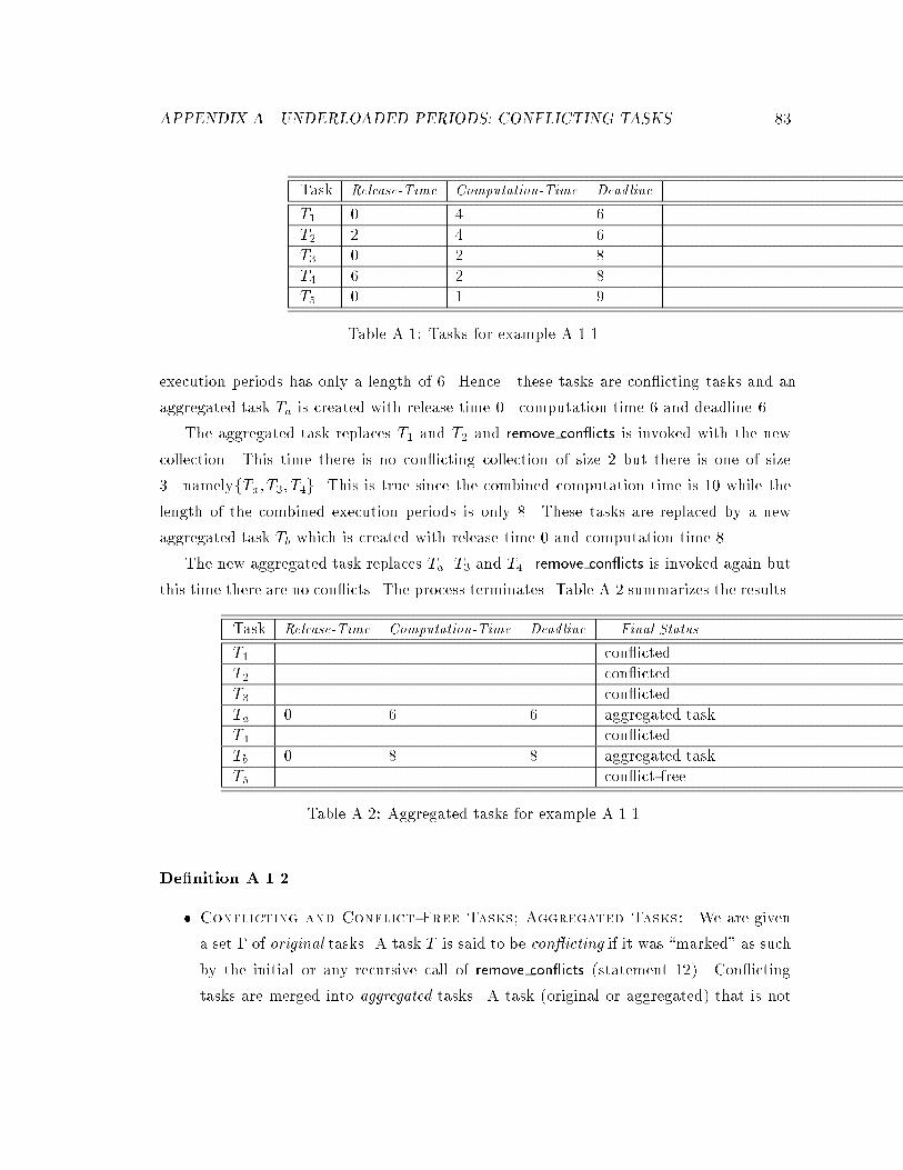
APPENDIX A. UNDERLOADED PERIODS: CONFLICTING TASKS 83
Task Release-Time Computation-Time Deadline
T1 0 4 6
T2 2 4 6
T3 0 2 8
T4 6 2 8
T5 0 1 9
Table A.1: Tasks for example A.1.1.
execution periods has only a length of 6. Hence these tasks are con icting tasks and an
aggregated task Ta is created with release time 0 computation time 6 and deadline 6.
The aggregated task replaces T1 and T2 and remove con icts is invoked with the new
collection. This time there is no con icting collection of size 2 but there is one of size
3 namelyfTa; T3; T4g. This is true since the combined computation time is 10 while the
length of the combined execution periods is only 8. These tasks are replaced by a new
aggregated task Tb which is created with release time 0 and computation time 8.
The new aggregated task replaces Ta T3 and T4. remove con icts is invoked again but
this time there are no con icts. The process terminates. Table A.2 summarizes the results.
Task Release-Time Computation-Time Deadline Final Status
T1 con icted
T2 con icted
T3 con icted
Ta 0 6 6 aggregated task
T4 con icted
Tb 0 8 8 aggregated task
T5 con ict-free
Table A.2: Aggregated tasks for example A.1.1.
De�nition A.1.2
� Conflicting and Conflict-Free Tasks; Aggregated Tasks: We are given
a set � of original tasks. A task T is said to be con icting if it was \marked" as such
by the initial or any recursive call of remove con icts (statement 12). Con icting
tasks are merged into aggregated tasks. A task (original or aggregated) that is not
APPENDIX A. UNDERLOADED PERIODS: CONFLICTING TASKS 84
con icting is said to be a con ict-free. When all the tasks (original or aggregated)
of a collection are con ict-free the collection is con ict-free and otherwise con icting.
A.1.1 The Performance Guarantee of Dover
In the following assume that a collection � is given.
Lemma A.1.1 � is overloaded if and only if it is con icting.
proof.
Assume � is con icting we will show that � is overloaded. Let T be the �rst aggregated
task to be created by remove con icts when invoked with � as its input. T is an aggregate
of original tasks. This means that the sum of the computation times needed for these tasks
is greater than the time between their earliest release and latest deadline (see statement
10 of remove con icts). Hence these tasks cannot be all scheduled. We conclude that � is
overloaded.
Assume � is overloaded we will show that � is con icting. Let � be a minimal set of
tasks in � that cannot be scheduled. � is minimal in the sense that removing any one task
will make the rest of the tasks in � schedulable3 . Let r be the earliest release time and d
the latest deadline among all tasks in � . Let � be scheduled by D.
Claim When D schedules � , there is no idle time between r and d.
Proof of claim.
Suppose the system is idle time at time t then at that time there is no ready task. This
means that � can be partitioned into two non-empty sets (one with all tasks with deadline
before t and the other with deadline after t). At least one of these sets cannot be scheduled4
contradicting the minimality of � .
End of proof of claim
Since the claim shows that there is no idle time and that D could not schedule all the
tasks even while executing continuously we conclude that the sum of computation times
needed for the tasks of � is greater than the time that can be possibly allotted to them.
Remove con icts must have found a con ict in �. To see this notice that as long as no
con ict is found the value of the variable collection num of tasks is advanced and is bound
3Such a minimal set must exists since the entire set of tasks � cannot be scheduled but every singletonset of tasks can be scheduled.
4Recall that D is an optimal scheduler for underloaded systems [28 7].
APPENDIX A. UNDERLOADED PERIODS: CONFLICTING TASKS 85
to reach the value of num of tasks(�). At that point all the tasks of � are still present (i.e.
were not merged into an aggregated task) and satisfy the condition of statement 10.
Hence � is con icting.
Lemma A.1.2 When scheduling �, D|the earliest-deadline-�rst algorithm| will sched-
ule to completion all con ict-free tasks.
proof.
Let C be the time that can be \occupied" by the aggregated tasks that is the pointwise
union of all their executable periods.
C = [Ti is an aggregated task[ri; di] (A.1)
One can verify (see statement 13 of remove con icts) that
C = [Ti is an (original) con icting task[ri; di] (A.2)
Remove con icts(�) contains all the con ict-free tasks. It is con ict-free otherwise re-
move con icts would not have halted. Hence by lemma A.1.1 all the tasks in
remove con icts(�) can be scheduled by D. The aggregated tasks of remove con icts(�)
cannot be scheduled outside C. Moreover all ofC must be occupied by aggregated tasks
since they have no slack time. Hence the con ict-free tasks are scheduled by D using only
time that lies outside C.
We showed that D schedules all the con ict-free tasks when the collection to be sched-
uled is remove con icts(�) but does this hold when D schedules the original set of tasks �?
The answer is yes. When scheduling � equation A.2 above shows that all the time outside
C is available to the con ict-free tasks hence by the previous paragraph all con ict-free
tasks complete their execution when � is scheduled by D.
Corollary A.1.3 D can schedule all the con icting-free tasks using only time outside C.
Lemma A.1.4 Suppose T is not the current executing task and is not in Q privileged. If T
has an earlier deadline than all the tasks in Q privileged and the current executing task (if
any), then T , the current executing task, and all the tasks in Q privileged can be scheduled
by D.
APPENDIX A. UNDERLOADED PERIODS: CONFLICTING TASKS 86
if and only if
availtime � remaining computation time(T )
proof.
The proof is by induction on the scheduling decisions of Dover. The induction is done
separately on each interval.
De�nition A.1.3
� Real LST Event : According to Dover scheduling when a task completion event
occurs the next task to be scheduled is the ready task T with the earliest-deadline.
It is possible that the slack-time of T reached zero exactly when a task completion
event occurred thus creating an LST event for T . We will call this LST event a
false event since T would have been scheduled even without the interrupt. All other
LST events will be called real.
In all of the following we ignore the false events. Only real LST events are considered.
Lemma A.1.5 1. Let C be the time that can be occupied by the aggregated tasks,
C = [Ti is an aggregated task[ri; di]
then, outside C, Dover schedules according to earliest-deadline-�rst (D).
2. Under Dover scheduling a con ict-free task will never generate a (real) latest-start-
time interrupt.
3. Let A be an aggregate task in remove con icts(�) with parameters (ra; da), then Dover
will complete on or before ra all con ict-free tasks with deadline on or before da.
proof.
Recall that the aggregated tasks in remove con icts(�) are those tasks that were created
\from" con icting tasks. List all the aggregated tasks according to deadline order
Ta1; Ta2; Ta3; � � �
By the construction of these tasks we know that
ra1 < da1 < ra2 < da2 < ra3 � � �
APPENDIX A. UNDERLOADED PERIODS: CONFLICTING TASKS 87
(Actually fromremove con icts one can infer only that da1 � ra2 but if it happens that
da1 = ra2 we can for the purpose of the the following proof merge Ta1 and Ta2 into one
aggregated task with parameters ra1
and da2)
Dover departs from the earliest-deadline-�rst scheduling policy only when one of the
following events occurs:
� The current task is lst-scheduled i.e. it was scheduled as the result of a latest-start-
time interrupt.
� At a task release event or at a task completion event the task with the earliest
deadline among all ready tasks is not scheduled because availtime is too small (see
statement 61 and 72 of Dover).
Dover starts to schedule according to earliest-deadline-�rst. Before ra1 there is no
con ict hence by lemma A.1.1 there is no overload. This means that neither of the above
conditions occurs (lemma A.1.4). Hence before the �rst aggregated task (up tora1) Dover
schedules in the same way as D. Also from corollary A.1.3 we conclude that all con ict-free
tasks with deadline on or before da1 completed on or before ra1 .
Between the �rst and second aggregated task i.e. between da1
and ra2
there cannot be
any ready con icting tasks because all con icting tasks have their deadlines before da1 or
release time after ra2. So during this time only con ict-free tasks are scheduled. Moreover
they will be scheduled according to earliest-deadline-�rst. We will show this by showing
that neither of the two cases above can hold. A con ict-free task would not create a real
LST event (corollary A.1.3 5). Also a task with the earliest-deadline will be immediately
scheduled. This holds because if it is delayed then D encounters an overloaded situation
while executing the con ict-free tasks outside C. This contradicts corollary A.1.3.
We conclude that up to ra2 Dover acts like D and all the con ict-free tasks with
deadline before da2 complete before ra2 . The induction can proceed through the entire list
of aggregated task and the lemma is proved.
Corollary A.1.6 Dover will schedule to completion all con ict-free tasks.
5As a matter of fact the con ict-free tasks might have even used some of the time of C (when scheduledby Dover).
APPENDIX A. UNDERLOADED PERIODS: CONFLICTING TASKS 88
Lemma A.1.7 Let A be an aggregate task in remove con icts(�) with parameters (ra; da),
then during (ra; da) a con ict-free task will be scheduled by Dover only if there are no ready
con icting tasks.
proof.
Lemma A.1.5 states that a con ict-free task with deadline on or before da would complete
before ra. So if any con ict-free task T with release time r and deadline d is to be scheduled
during A it must satisfy d > da.
Suppose at time t 2 (ra; da) there is a ready con icting task Ti. Then di < da must
hold becauseTi must be a part of the aggregated task A 6 7.
Hence at timet all ready con icting tasks have deadlines before the deadline of any
con ict-free task. A con ict-free task can be scheduled in these circumstances only by a
latest-start-time interrupt. This cannot occur because a con ict-free task will not generate
a (real) latest-start-time interrupt (lemma A.1.5)
Theorem A.1.8 Dover schedules to completion all con ict-free tasks and obtains at least1
(1+pk)2
the value a clairvoyant algorithm gets from all other (i.e., con icting) tasks.
proof.
The �rst part of this lemma is merely a repetition of corollary A.1.6. From lemma A.1.7 we
conclude that Dover schedules the con icting tasks regardless the presence of the con ict-
free tasks. Suppose the clairvoyant algorithm has to schedule only the con icted-tasks. It
can schedule this tasks only during C. But we have just shown that Dover schedules the
con icted tasks as if the con ict-free tasks do not exist. Since Dover has a competitive
multiplier of (1 +pk)2 it is guaranteed to achieve at least 1
(1+pk)2
of what a clairvoyant
algorithm can achieve from all con icting tasks.
6We say that a taskT is a part of an aggregated task A if it is one of the tasks that were \merged" tocreate A.
7Ti is a con icting task hence it is a part of some aggregated task B if this task is notA then the
two aggregated tasks should be merged contradicting the fact that A is a task in remove con icts(�) henceA = B.
Appendix B
Dover: Gradual Descent
89
APPENDIX B. DOVER
: GRADUAL DESCENT 90
In the previous sections we assumed �rm deadlines. That is a task has zero value if it
misses its deadline. We would like to generalize to soft deadlines which means that a task
may have some value even after its deadline.
We assume here a soft deadline scheme called gradual descent and show that a suitable
variant of Dover is (1 +pk)2 competitive in this case. Dover is also (1 +
pk)2 competitive
in some possible generalizations of this scheme. We discuss these generalizations at the
end of this appendix.
B.1 Exponential Gradual Descent
Consider the following \exponential" value assignment for gradual descent. If a task Ti
with computation time ci and value vi does not complete by its deadline di (we call this
deadline thezeroth deadline and denote it by d0i ) then a value of vi2 can be obtained if
it completes by di +ci2 . This \deadline" is denoted by d1i . In general a value of vi
2y is
obtained the task completes by its y'th deadline dyi = di +
ci2 + ci
4 + � � �+ ci2y . We keep
the list of deadlines �nite by postulating that a task's value density cannot go below 1.
This means that the index of the last deadline after which the tasks has zero value is
blog2(value density(Ti))c � 1 = blog2(vici )c � 1.
For notational convenience any task Ti will have associated descending tasks denoted
by
T 0i ; T
1i ; T
2i ; � � � ; T blog2(imp(Ti))c�1
i
where the release times and the computation times of all these tasks are equal to the
release time and the computation time of Ti. Tyi has a �rm deadline at d
yi and a value of
vi2y . Only one of the tasks associated with Ti can possibly complete. That is if we say that
an algorithm executes Tyi we mean that Ti completes by deadline d
yi but after deadline
dy�1i .
B.2 A Variant of Dover for Gradual Descent
We modify the latest-start-time interrupt handler of Dover in such a way that when T 0i
is to be abandoned because it reached its LST but does not have enough value to be
scheduled (see statement 89 of Dover) T 0i is indeed removed from all the data structures
APPENDIX B. DOVER
: GRADUAL DESCENT 91
but in addition a task release for T 1
i is simulated. T 1
i 's remaining computation time is set
to the remaining computation time of T 0
i . In the same way ifT 1
i is to be abandoned then
a third task is \released". This process continues as long as the value density does not go
below 1.
B.3 Analysis of Dover in the Gradual Descent Model
The analysis is similar to one in section 3.2. We will discuss the di�erences only. Suppose
that a collection of tasks � with importance ratio k is given and that Dover schedules
this collection. We partition the collection of tasks according to the question of which
associated tasks (if any) completed.
� Let Sp denote the set of tasks that completed successfully and that ended some
positive time before their zeroth deadline.
� Let S0 denote the set of tasks that completed successfully but ended exactly at their
zeroth deadline.
� For 1 � y � blog2kc � 1 letSy denote the set of tasks that completed successfully
after their (y�1)'th deadline but not after their y'th deadline (i.e. they'th associated
task completed).
� Let FAIL denote the set of tasks that never completed.
We will start by modifying the technical lemmas of subsection 3.2.2 to the new setting.
B.3.1 Lemmas about Dover's Scheduling
For notational convenience we de�ne a minus one deadline d�1i which equals to the zeroth
deadline d0i .
�In this setting lemma 3.2.2 reads
Lemma B.3.1
1. For any task Ti in Sy (with y � 0). Suppose Tyi completed at time tcomplete � d
yi ,
then
[ri; dy�1i ] � [ri; tcomplete] � BUSY
APPENDIX B. DOVER
: GRADUAL DESCENT 92
2. For any task Ti in FAIL. Suppose Ti was abandoned at time taban, then
[ri; taban] � BUSY
proof.
The proof is similar to that of lemma 3.2.2.
�Lemma 3.2.3 holds without change. Note that we continue to make the normalized
importance assumption because we never allow the value density to fall below 1.
�Lemma 3.2.4 holds without change.
�Lemma 3.2.5 reads:
Lemma B.3.2 Suppose Tyi was abandoned at time t in I = [tbegin; tclose]. Then,
ci � dyi � tclose
proof.
The proof is the same as the proof of lemma 3.2.5.
B.3.2 How Well Can a Clairvoyant Scheduler Do?
As in subsection 3.2.3 given a collection of tasks � our goal is to bound the maximum value
that a clairvoyant algorithm can obtain from scheduling �. We observe the scheduling of
� by Dover which gives rise to the de�nition of Sp theSy 's and FAIL. As before BUSY
is de�ned to be the union of the periods in which the processor was not idle (under Dover 's
scheduling).
The clairvoyant algorithm is o�ered the same two gifts as before. The �rst is the sum
of the values of all tasks in Sp at no cost to it. The second gift is the granted value. That
is in addition to the value obtained from scheduling
LATE = (S0[ S1
[ � � �Sblog2kc�1 [ FAIL)
a value density of k will be granted for every period of BUSY that is not used for executing
APPENDIX B. DOVER
: GRADUAL DESCENT 93
a task of LATE. By a similar argument to lemma 3.2.6 we can see that1
C(LATE) � max
possible
scheduling
of LATE
8>>>>><>>>>>:
value obtained by
scheduling tasks of
LATE
+ k �length of time in BUSY not
utilized by tasks of LATE
9>>>>>=>>>>>;
In lemma 3.2.8 we bounded the net gain that the clairvoyant algorithm could get from
scheduling tasks of F 2. This was done by examining each interval separately. If T 2 F is
scheduled then its value is accounted for in the interval in which T was abandoned by Dover .
Here the method of relating the value of a task T 2 LATE to the interval in which it is
accounted for is more complicated. Suppose the clairvoyant algorithm chose to execute the
z'th task of Ti to completion. Dover could have chosen to complete any of the associated
tasks of Ti (Ti 2 Sy for some y) or none (Ti 2 FAIL). In the �rst case we account for
T zi in the interval in which Dover completed Ti; in the second case in the interval during
which T zi was abandoned.
Assume that a clairvoyant scheduler selected an optimal scheduling for the tasks of
LATE considering the value that can be gained from leaving BUSY periods idle. The
execution of a task can give a positive net gain only if the task executed (at least partially)
outside BUSY . The following lemma shows that such execution may take place only after
tclose.
Lemma B.3.3 Suppose the associated task T zi of Ti 2 LATE is scheduled to completion
by the clairvoyant algorithm. Suppose that Ti is accounted for in I = [tbegin; tclose]. Then,
if Ti is to be executed (by the clairvoyant algorithm) anywhere outside BUSY it must be
after tclose.
proof.
There are two cases:1Recall that C(FAIL) denotes the value that a clairvoyant algorithm can achieve from scheduling
LATE.2Note that in section 3.2 the clairvoyant scheduler could not make any net gain from tasks of S0 that
completed in I because they can be executed only during BUSY . This is not the case here because ifTyi completed in I the clairvoyant algorithm could choose a di�erent completion point for T y
i or even toabandon it in favor of another associated task T z
i with z 6= y.
APPENDIX B. DOVER
: GRADUAL DESCENT 94
� Dover never completed Ti (Ti 2 FAIL). In this case let t be the time when Dover
abandoned T zi .
T zi can be executed only during �T z
iwhich is is [ri; t] [ [t; dzi ]. The �rst portion of
�T ziis contained in BUSY (lemma B.3.1). The second portion is contained in I .
Hence [ri; tclose] � BUSY .
� Dover completed Tyi for some y. Let t be the completion time of T y
i .
A similar argument as above for �Tyi= [ri; t][ [t; dyi ] shows that [ri; tclose] � BUSY .
Hence in both cases ifT zi is to be executed outside BUSY it must be after tclose .
�Lemma 3.2.8 has to be replaced by the following
Lemma B.3.4 With the above gifts, the total net gain obtained by the clairvoyant algo-
rithm from scheduling the (associated) tasks accounted for in I is not greater than
(1 +pk) � achievedvalue(I)
proof.
Let T1; T2; � � �Tm be those tasks that are accounted for in I = [tbegin; tclose] and that the
clairvoyant algorithm scheduled after tclose (in order of completion). These tasks execute
for l1; l2; � � � lm time after tclose (hence maybe outside BUSY by the above lemma).
Denote by L the following value
L = maxf(1 +pk) � achievedvalue(I)
k; l1g (B.1)
Let j be the index less than or equal to m such that
X
i�j
li � L < lj+1 +X
i�j
li
If no such j exists de�ne j to be m.
First assume that we have an equalityP
i�j li = L.
The proof now has two parts.
}Part 1 :
We will show that the net gain from scheduling tasks within a period of L after the end of
the interval cannot be greater than (1 +pk) � achievedvalue(I).
APPENDIX B. DOVER
: GRADUAL DESCENT 95
� Suppose that in B.1 the maximum is the �rst term. Then the total net gain from
T1; T2; � � �Tj is not greater thank �X
i�j
li = k � L = (1 +pk) � achievedvalue(I) (B.2)
� Suppose the second term is maximum in B.1 and that the z'th associated task of T1
was scheduled by the clairvoyant algorithm. If T z1was abandoned in I (by Dover) then
lemma 3.2.4 ensures that its value is bounded by (1+pk)�achievedvalue(I). The other
possibility is that Dover completed Ty1in I . If z � y then value(T z
1) � value(T y
1) but
value(T y1) is a component of achievedvalue(I) so must be less or equal to it. z < y
implies that T1 executed to completion (by the clairvoyant algorithm) before tclose
since dzi < dyi � tclose | a contradiction.
Hence in any case the value obtained by scheduling T1 is at most
(1 +pk) � achievedvalue(I).
}Part 2 :
Now we will show that the net gain from scheduling a task Ti (j < i � m) L time after
the end of I is never positive. Here we have to distinguish between two cases depending
on whether Dover completed or abandoned Ti in I .
� Dover completed Ti
Suppose that Dover completed Tyi at tcomplete 2 I and that the clairvoyant algorithm
chose to schedule T zi .
There are two possible cases:
{ z < y:
Lemma B.3.1 shows that
[ri; dzi ] � [ri; tcomplete] � BUSY
This means that T zi executes during BUSY a contradiction.
{ z � y:
The gradual descending scheme ensures that
dzi = d0i +ci
2+
ci
4+ � � �+ ci
2z
= d0i + (ci � ci
2z)
APPENDIX B. DOVER
: GRADUAL DESCENT 96
From lemma B.3.1 we see that
d0i � dy�1i � tcomplete � tclose 2 BUSY
Hence we conclude that
dzi � tclose + (ci �ci
2z)
T zi must complete at or before dzi implying that the clairvoyant algorithm sched-
ules T zi for at least ci
2ztime before tclose hence in BUSY . The loss from the
execution during BUSY is at least ci2z�k while the value of T z
i is at most ci�k2z
.
Hence the net gain is not positive.
� Ti 2 FAIL
Suppose that the y'th associated task of Ti was scheduled by the clairvoyant algorithm
and that Tyi was abandoned by Dover in I = [tbegin; tclose]. T
yi has an execution time
of at least dyi � tclose by lemma B.3.2.
dyi � tclose
� \the point at which Tyi completes (according to the clairvoyant)"� tclose
� (tclose +X
g�i
lg)� tclose
� li +X
g�j
lg = li + L
Tyi was scheduled by the clairvoyant scheduler but used only li time after tclose .
Hence Ti executed at least L time before tclose that is to say in BUSY (lemma B.3.3).
The \loss" from scheduling Ti during BUSY is at least k � L. The value obtained
by scheduling Ti is at most (1+pk) � achievedvalue(I) (lemma 3.2.4). Hence the net
gain is less than or equal to
(1 +pk) � achievedvalue(I)� k �L
� (1 +pk) � achievedvalue(I)� (1 +
pk) � achievedvalue(I)
= 0
What if L does not equal any of the partial sums? That is ifP
i�j li < L <P
i�j+1 li. As
in the proof of lemma 3.2.8 we augment the total value given to the clairvoyant by some
APPENDIX B. DOVER
: GRADUAL DESCENT 97
non-negative amount. Even with this addition the net gain achieved by the clairvoyant
algorithm is bounded by (1 +pk) � achievedvalue(I) hence proving the lemma.
�Corollary 3.2.9 holds with LATE replacing F .
Before we continue we must clarify the meaning of poslaxval and zerolaxval in this
setting. poslaxval denotes the value obtained by tasks that completed before their zeroth
deadline (tasks in Sp). zerolaxval denotes the total value obtained by tasks that completed
at or after that deadline (i.e. tasks inS0 [ S1 [ � � �Sblog2kc�1).�Lemma 3.2.10 holds without change given these new de�nitions of poslaxval and zerolaxval.
�Lemma 3.2.11 holds with LATE replacing F [ S0.
Theorem B.3.5 In the exponential gradual descent model, Dover has a competitive mul-
tiplier of (1 +pk)2.
proof.
Proof as in theorem 3.2.12.
B.4 Inherent Bounds
The inherent bound given by Baruah et. al. [4 3] cannot be directly applied here. Hence
it is not clear whether Dover is optimal in this setting. It might very well be that the
introduction of descending value schemes helps the on-line scheduler more then it helps
the clairvoyant one. Thus the question of �nding the inherent bounds in this case is open.
B.5 Performance Guarantee for Underloaded Periods
In the gradual descent model we de�ne an underloaded collection of tasks as a collection
such that all its tasks can be scheduled by the zeroth deadline (i.e. with their full value).
It is clear that Dover will get 100% of the value for such a collection since it will execute
according to earliest deadline �rst scheduling.
B.6 Other Gradual Descent Schemes
In this section we presented a speci�c scheme of gradual descent. In fact the current
argument can provide the same result for more general schemes of descending value.
APPENDIX B. DOVER
: GRADUAL DESCENT 98
All schemes must have the following properties:
� The value density of a task must not go below 1 (used in lemma 3.2.3).
� For every possible associated task T ziof Ti
dz
i < d0
i + ci
and
(dzi � d0
i )� k � \the value of T zi"
(used in part 2 of lemma B.3.4)
Within these constraints many schemes are possible. Some tasks can have �rm dead-
lines; others obtain values that decrease monotonically as the distance from the deadline
increases. The base of the exponent (Base 2 used here is an arbitrary choice) can be
di�erent for di�erent tasks.
Appendix C
Dover: Exact Computation Time
Is Not Known
99
APPENDIX C. DOVER
: EXACT COMPUTATION TIME IS NOT KNOWN 100
Suppose the on-line scheduling algorithm is not given the exact computation time of a task
upon its release. However for every task Ti an upper bound on its possible computation
time denoted by ci;max is given. Also the actual computation time ofTi denoted by ci
satis�es:
(1� �) � ci;max � ci � ci;max
Where 0� � < 1 is a given error margin which is common to all the tasks. We make
the following additional assumptions:
Assumption C.0.1
� The Actual Computation Time Is Environment-Invariant: The actual com-
putation time of a task does not depend on the point in time in which it was scheduled
the number of times it was preempted and rescheduled etc.
� The Actual Computation Time Is Not Known Before The Completion
Point: An on-line scheduler cannot know the exact computation time of a task
until it completes.
Some terms has to be rede�ned in the new set up:
De�nition C.0.2
� Underloaded Collection of Tasks: A collection of tasks is underloaded (in
this setting) if the actual computation times enable execution of all the tasks to
completion.
� Importance Ratio: The importance ratio k of a collection with an error margin
of � is de�ned to be the ratio of the largest possible value density to the smallest
possible value density.
k =maxi
vi(1��)�ci;max
minivi
ci;max
=1
(1� �)�maxi
vici;max
minivi
ci;max
(C.1)
Here thenormalized importance assumption (assumption 2.0.2) means that
mini
vi
ci;max
� 1
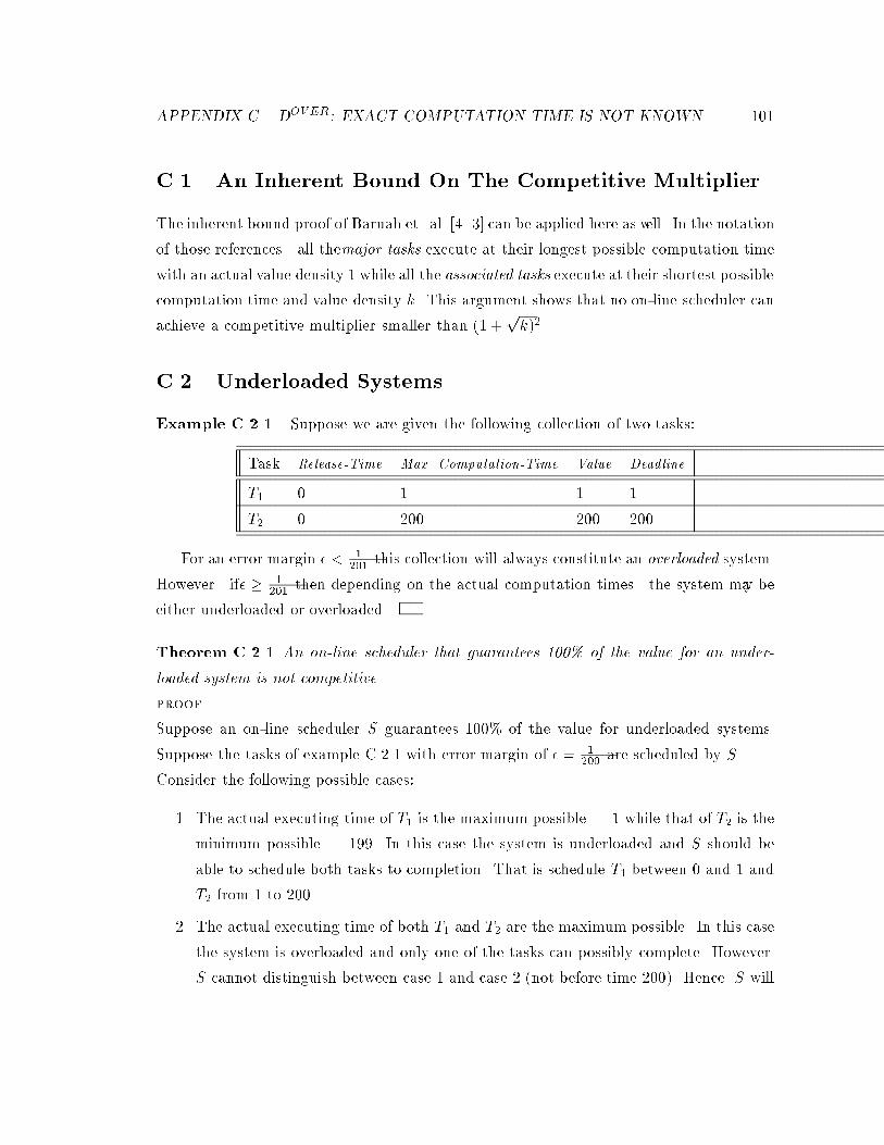
APPENDIX C. DOVER
: EXACT COMPUTATION TIME IS NOT KNOWN 101
C.1 An Inherent Bound On The Competitive Multiplier
The inherent bound proof of Baruah et. al. [4 3] can be applied here as well. In the notation
of those references all themajor tasks execute at their longest possible computation time
with an actual value density 1 while all the associated tasks execute at their shortest possible
computation time and value density k. This argument shows that no on-line scheduler can
achieve a competitive multiplier smaller than (1 +pk)2.
C.2 Underloaded Systems
Example C.2.1 Suppose we are given the following collection of two tasks:
Task Release-Time Max. Computation-Time Value Deadline
T1 0 1 1 1
T2 0 200 200 200
For an error margin � < 1
201this collection will always constitute an overloaded system.
However if� � 1
201then depending on the actual computation times the system may be
either underloaded or overloaded.
Theorem C.2.1 An on-line scheduler that guarantees 100% of the value for an under-
loaded system is not competitive.
proof.
Suppose an on-line scheduler S guarantees 100% of the value for underloaded systems.
Suppose the tasks of example C.2.1 with error margin of � = 1
200are scheduled by S.
Consider the following possible cases:
1. The actual executing time of T1 is the maximum possible | 1 while that of T2 is the
minimum possible | 199. In this case the system is underloaded and S should be
able to schedule both tasks to completion. That is schedule T1 between 0 and 1 and
T2 from 1 to 200.
2. The actual executing time of both T1 and T2 are the maximum possible. In this case
the system is overloaded and only one of the tasks can possibly complete. However
S cannot distinguish between case 1 and case 2 (not before time 200). Hence S will
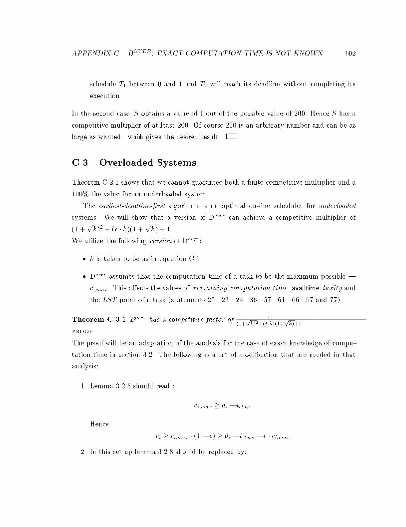
APPENDIX C. DOVER
: EXACT COMPUTATION TIME IS NOT KNOWN 102
schedule T1 between 0 and 1 and T2 will reach its deadline without completing its
execution.
In the second case S obtains a value of 1 out of the possible value of 200. Hence S has a
competitive multiplier of at least 200. Of course 200 is an arbitrary number and can be as
large as wanted which gives the desired result.
C.3 Overloaded Systems
Theorem C.2.1 shows that we cannot guarantee both a �nite competitive multiplier and a
100% the value for an underloaded system.
The earliest-deadline-�rst algorithm is an optimal on-line scheduler for underloaded
systems. We will show that a version of Dover can achieve a competitive multiplier of
(1 +pk)2 + (� � k)(1 +
pk) + 1.
We utilize the following version of Dover :
� k is taken to be as in equation C.1.
� Dover assumes that the computation time of a task to be the maximum possible |
c�;max. This a�ects the values of remaining computation time availtime laxity and
the LST point of a task (statements 20 23 24 36 57 61 66 67 and 77).
Theorem C.3.1 Dover has a competitive factor of 1(1+
pk)2+(��k)(1+
pk)+1
proof.
The proof will be an adaptation of the analysis for the case of exact knowledge of compu-
tation time in section 3.2. The following is a list of modi�cation that are needed in that
analysis:
1. Lemma 3.2.5 should read :
ci;max � di � tclose
Hence
ci � ci;max � (1� �) � di � tclose � � � ci;max
2. In this set up lemma 3.2.8 should be replaced by:
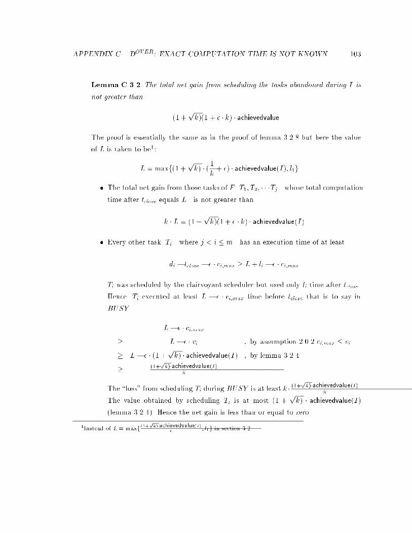
APPENDIX C. DOVER
: EXACT COMPUTATION TIME IS NOT KNOWN 103
Lemma C.3.2 The total net gain from scheduling the tasks abandoned during I is
not greater than
(1 +pk)(1 + � � k) � achievedvalue
The proof is essentially the same as in the proof of lemma 3.2.8 but here the value
of L is taken to be1:
L = maxf(1 +pk) � (1
k+ �) � achievedvalue(I); l1g
� The total net gain from those tasks of F T1; T2; � � �Tj whose total computation
time after tclose equals L is not greater than
k � L = (1 +pk)(1 + � � k) � achievedvalue(I)
� Every other task Ti where j < i � m has an execution time of at least
di � tclose � � � ci;max � L+ li � � � ci;max
Ti was scheduled by the clairvoyant scheduler but used only li time after tclose .
Hence Ti executed at least L � � � ci;max time before tclose that is to say in
BUSY .
L� � � ci;max
� L� � � vi ; by assumption 2.0.2 ci;max � vi
� L� � � (1 +pk) � achievedvalue(I) ; by lemma 3.2.4
� (1+pk)�achievedvalue(I)
k
The \loss" from scheduling Ti during BUSY is at least k � (1+pk)�achievedvalue(I)
k.
The value obtained by scheduling Ti is at most (1 +pk) � achievedvalue(I)
(lemma 3.2.4). Hence the net gain is less than or equal to zero.
1Instead of L = maxf (1+
pk)�achievedvalue(I)
k; l1g in section 3.2
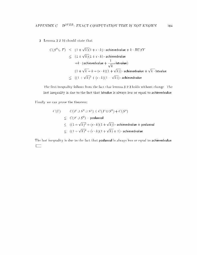
APPENDIX C. DOVER
: EXACT COMPUTATION TIME IS NOT KNOWN 104
3. Lemma 3.2.10 should state that
C(S0[ F ) � (1 +
pk)(1 + � � k) � achievedvalue + k �BUSY
� (1 +pk)(1 + � � k) � achievedvalue
+k � (achievedvalue + 1pk� lstvalue)
= (1 +pk + k + (� � k)(1 +
pk)) � achievedvalue +
pk � lstvalue
� ((1 +pk)2 + (� � k)(1 +
pk)) � achievedvalue
The �rst inequality follows from the fact that lemma 3.2.3 holds without change. The
last inequality is due to the fact that lstvalue is always less or equal to achievedvalue.
Finally we can prove the theorem:
C(�) = C(F [ S0 [ Sp) � C(F [ S0) + C(Sp)
� C(F [ S0) + poslaxval
� ((1 +pk)2 + (� � k)(1 +
pk)) � achievedvalue + poslaxval
� ((1 +pk)2 + (� � k)(1 +
pk) + 1) � achievedvalue
The last inequality is due to the fact that poslaxval is always less or equal to achievedvalue.
Appendix D
Two Processor Systems
105
APPENDIX D. TWO PROCESSOR SYSTEMS 106
This appendix deals with systems having only two processors. We also assume uniform
value density (i.e. n = 2; k = 1). With out loss of generality we can assume that the value
density is normalized to 1. We consider two possible models of multiprocessor systems.
In the �rst model tasks canmigrate cheaply (and quickly) from one processor to another.
Hence if a task started to execute on one processor it can later continue on any other
processor (and migration takes no time). We present a scheduling algorithm called the
Safe-Risky algorithm for this model. In the second model (the �xed model) once a task
starts to execute on one processor it cannot execute on any other processor. An on-line
scheduler can do better when migration is possible.
D.1 The Safe-Risky Algorithm
In this algorithm one processor is designated as theSafe Processor (SP) and the other
as the Risky Processor (RP). A task that started to execute on SP is called \privileged"
because it is guaranteed to complete (Q privileged is a queue containing these tasks).
Ready tasks that are not privileged wait in Q waiting until they become privileged
or they reach their LST at that point the LST task tries to be scheduled on RP. It will
be scheduled if it has a bigger value than the task currently executing on RP. A task
that started to execute on RP can be preempted and then resume on SP (i.e. migrate to
SP). In this version of the algorithm the designation as safe or risky processor is �xed. In
the no-migration version (the Safe-Risky-(�xed)) the processors may switch roles. The
following few boxes (�gures D.1- D.2) depict the code of the Safe-Risky algorithm:
Remark D.1.1 All privileged tasks should be able to complete using only a single proces-
sor at a time. This mean that the privileged tasks constitute a uniprocessor underloaded
system. A new task is accepted to Q privileged only if it does not create an overload when
added to the tasks already in Q privileged .
Note an important di�erence between the above algorithm (and for that matter also
Dover and the version of theMOCA Algorithm presented earlier. In the task release routine
a newly arrived tasks will be added to Q privileged only if its deadline is earlier than the
currently executing task and also it can be added toQ privileged without creating overload
(we call that a local schedulability test). This stands in contrast to the global schedulability
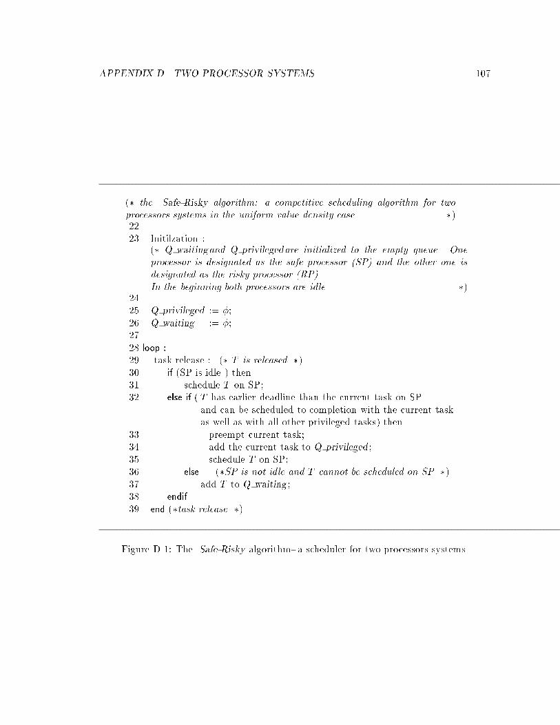
APPENDIX D. TWO PROCESSOR SYSTEMS 107
(� the Safe-Risky algorithm: a competitive scheduling algorithm for twoprocessors systems in the uniform value density case �)2223 Initilzation :
(� Q waitingand Q privilegedare initialized to the empty queue. Oneprocessor is designated as the safe processor (SP) and the other one isdesignated as the risky processor (RP).In the beginning both processors are idle. �)
2425 Q privileged := �;26 Q waiting := �;2728 loop :29 task release : (� T is released �)30 if (SP is idle ) then31 schedule T on SP;32 else if ( T has earlier deadline than the current task on SP
and can be scheduled to completion with the current taskas well as with all other privileged tasks) then
33 preempt current task;34 add the current task to Q privileged ;35 schedule T on SP;36 else (�SP is not idle and T cannot be scheduled on SP �)37 add T to Q waiting ;38 endif
39 end (�task release �)
Figure D.1: The Safe-Risky algorithm- a scheduler for two processors systems.
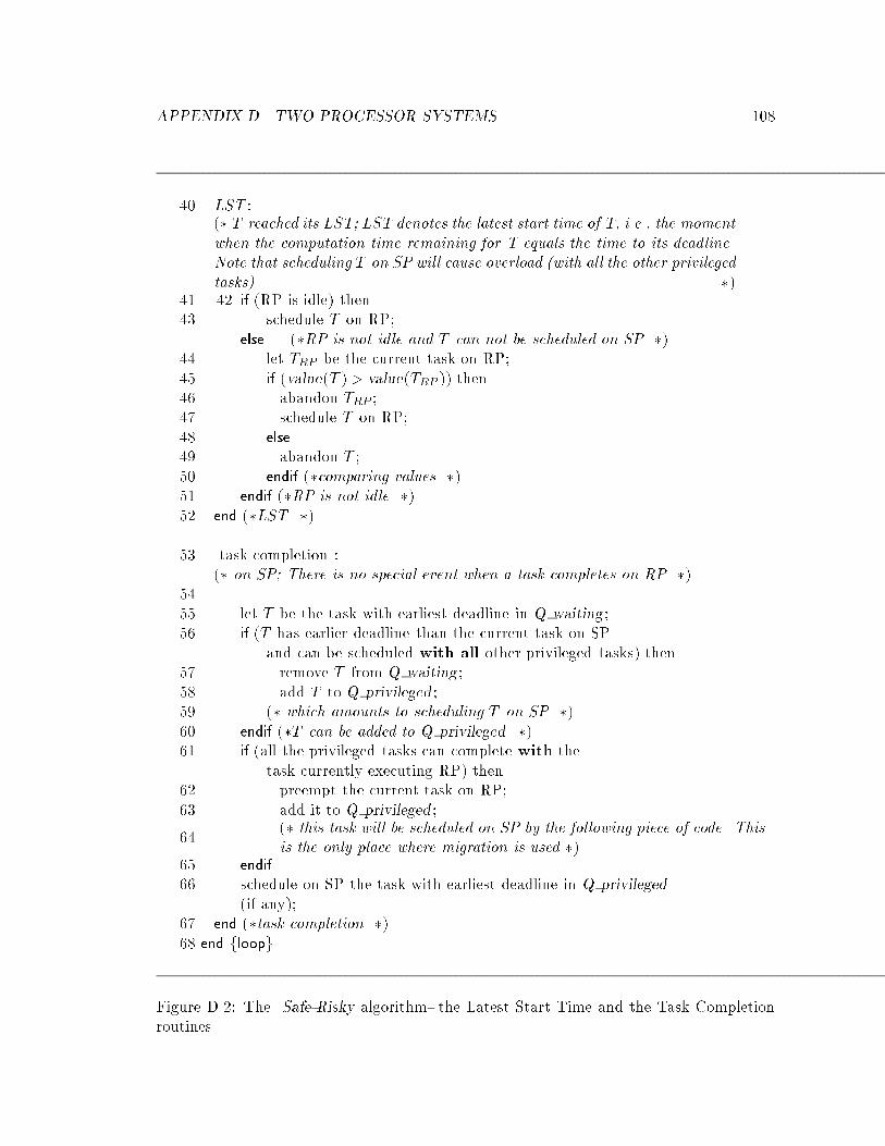
APPENDIX D. TWO PROCESSOR SYSTEMS 108
40 LST :(� T reached its LST; LST denotes the latest start time of T, i.e., the momentwhen the computation time remaining for T equals the time to its deadlineNote that scheduling T on SP will cause overload (with all the other privilegedtasks) �)
41 42 if (RP is idle) then43 schedule T on RP;
else (�RP is not idle and T can not be scheduled on SP �)44 let TRP be the current task on RP;45 if (value(T ) > value(TRP )) then46 abandon TRP ;47 schedule T on RP;48 else
49 abandon T ;50 endif (�comparing values �)51 endif (�RP is not idle �)52 end (�LST �)
53 task completion :(� on SP; There is no special event when a task completes on RP �)
5455 let T be the task with earliest deadline in Q waiting ;56 if (T has earlier deadline than the current task on SP
and can be scheduled with all other privileged tasks) then57 remove T from Q waiting ;58 add T to Q privileged ;59 (� which amounts to scheduling T on SP �)60 endif (�T can be added to Q privileged �)61 if (all the privileged tasks can complete with the
task currently executing RP) then62 preempt the current task on RP;63 add it to Q privileged ;
64(� this task will be scheduled on SP by the following piece of code. Thisis the only place where migration is used �)
65 endif
66 schedule on SP the task with earliest deadline in Q privileged
(if any);67 end (�task completion �)68 end floopg
Figure D.2: The Safe-Risky algorithm- the Latest Start Time and the Task Completionroutines.
APPENDIX D. TWO PROCESSOR SYSTEMS 109
task used by the MOCA Algorithm. That is: a new task enters Q privileged if and only if
it does not create overload irrespectively of its deadline.
D.2 The Competitive Multiplier of the Safe-Risky algo-
rithm
In this section we show that the Safe-Risky algorithm has a competitive multiplier of
2. Our approach is to partition the execution into disjoint intervals the Safe-Risky
algorithmgets at least half the optimal value in each interval. This is proved by means
of \covering". We show that all intervals are covered; if a period is covered then the
Safe-Risky algorithmuses at least one processor productively during all that period. The
clairvoyant scheduler could gain a factor of two by utilizing both processors.
De�nition D.2.1
� earliness, latest affected, cover end: By de�nition the tasks of Q privileged
constitute an underloaded subsystem (i.e all these tasks can complete onone pro-
cessor).
Now let us consider one additional task T which has a deadline earlier than all the
tasks in Q privileged . Suppose that the system comprised of Q privileged plus T is
overloaded. We want to know which of the tasks of Q privileged con ict with T .
Compute the earliness of all the tasks in Q privileged . That is suppose the tasks are
scheduled according to the earliest-deadline-�rst scheduling algorithm the earliness
of a task is how much before its deadline it completes (i.e its deadline minus its
completion time). Any task with earliness smaller than T 's computation time in
Q privileged prevents T from being added to Q privileged .
De�ne latest a�ected(T ) to be the latest deadline of any such task (i.e a tasks whose
earliness is smaller than T 's computation time) and de�ne cover end(T ) to be
cover end(T )def= maxfdeadline(T ); latest a�ected(T )g
� interval: An interval starts when a task is released to an idle system (the system
becomes non-idle) and ends when the system becomes idle again (both processors
are idle).
APPENDIX D. TWO PROCESSOR SYSTEMS 110
In the following we are going to analyze the Safe-Risky algorithm interval by interval.
For the sake of notational convenience let us assume that there was only one interval (call
it I) and it started at time 0.
Lemma D.2.1 The value obtained by the Safe-Risky algorithm from tasks executed on
SP during an interval is at least the interval length (duration).
proof.
From the beginning of the interval to its end SP is never idle (when SP is idle so is RP
which means that the interval ends). A task that was scheduled on SP is guaranteed to
complete. We conclude that at any given moment at least one processor is working on a
task that will eventually complete. This proves the lemma.
Notation D.2.2
� C(I), V(I)
For an interval I letC(I) and V (I) denote the value obtained by the clairvoyant
algorithm and the Safe-Risky algorithm (respectively) from tasks released during I .
De�nition D.2.3
� conflicted task, max cover: We say that T is a con icted task if it con icts
with the tasks of Q privileged (when considered for execution at the task release
routine, task completion routine or the LST routine, see statements 32, 56 and 41)
and hence was diverted to RP (and later was either scheduled to execution or was
abandoned).
De�ne max cover as,
max cover = max cover(I)def= max
T is a
con icted task
cover end(T )
If there is no con icted task this max equals 0.
We are going to show that for every task that was abandoned1 SP was productive during
its entire executable period. This is true for all the tasks that were abandoned during some
1Every task that was abandoned is a con icted-task.
APPENDIX D. TWO PROCESSOR SYSTEMS 111
interval. Hence the Safe-Risky algorithm gets a value of at least the union of all these
periods that is max cover.
Lemma D.2.2 For every task T , if T is a con icted task (i.e, was diverted to RP by the
Safe-Risky algorithm) then2, the total value obtained by the Safe-Risky algorithm is at
least cover end(T ).
proof.
Recall that cover end(T ) = maxfdeadline(T ); latest a�ected(T )g
� First let us show that V (I) � deadline(T ).
T is diverted to RP at its latest start time which is at deadline(T )
�computation time(T ). This means that the interval length is at least deadline(T )�
computation time(T ) (recall that the interval starts at time 0). Lemma D.2.1 says
that the value obtained by the Safe-Risky algorithm on SP is at least deadline(T )�
computation time(T ).
If T does not complete it can be abandoned only in favor of a bigger valued task
(scheduled on RP) hence the value obtained is at least value(T ). Hence
V (I) � (deadline(T )� computation time(T )) + value(T )
= (deadline(T )� computation time(T )) + computation time(T )
= deadline(T )
� Now we are going to show that V (I) � latest a�ected(T ).
By de�nition latest a�ected(T) is the deadline of some privileged task Taffected. Let
tactual be the time when Taffected completed (according to the Safe-Risky algorithm).
tactual cannot be any earlier than the estimated completion time of Taffected computed
when T was considered for execution (the actual time can be in fact later than the
estimated time if some tasks were later added to Q privileged). The length of the
interval is at least tactual. Lemma D.2.1 shows that the value obtained on SP is at
least this length.
As mentioned before the Safe-Risky algorithm an additional value of at least
value(T ). Hence
V (I) � tactual + computation time(T )
2Recall that the interval starts at time 0.
APPENDIX D. TWO PROCESSOR SYSTEMS 112
� deadline(Taffected)
= latest a�ected(T )
The second inequality restates the de�nition of latest a�ected(T).
Corollary D.2.3 The value obtained by the Safe-Risky algorithm during an interval is
at least
maxfthe interval length;max coverg
De�nition D.2.4
� covered, uncovered, atomic interval: For any interval I letuncovered =
uncovered(I) be the set of tasks (released in I) with deadlines after max cover(I).
Denote the remaining tasks by covered = covered(I). I is called an atomic interval
if uncovered(I) = � (the empty set).
We will show that during the �rst portion of an interval (from 0 tomax cover) the Safe-
Risky algorithm gets a value of at least one half the value obtainable from the tasks of
covered. If there are other tasks (i.e. tasks ofuncovered) then they are all going to complete
successfully without competing with covered tasks (either before or after max cover).
Lemma D.2.4 For an atomic interval I,
C(I) � 2V (I)
proof.
All tasks have deadlines before max cover. So the best the clairvoyant algorithm can do is
to schedule tasks on both processors from time 0 tomax cover to get a value of 2�max cover.
Corollary D.2.3 ensure that the Safe-Risky algorithm gets a value of max cover at least.
APPENDIX D. TWO PROCESSOR SYSTEMS 113
Now we are ready to extend the above lemma to a general interval. We are going to
use induction. The result is already given for atomic interval. We will show that a general
interval can be broken into atomic intervals and \uncovered" periods between them. The
covered tasks \cover" the atomic intervals. That is they generate value of at least the
combined length of these intervals. The tasks of uncovered execute without interfering
with the covered task and generate value of at least the length of the uncovered periods.
Lemma D.2.5 For every non atomic interval, I,
� All the tasks of uncovered are executed to completion on SP.
� When a task of uncovered is executing on SP, RP is idle.
� Suppose the tasks of uncovered were never released (i.e, only the tasks of covered were
released). Then, the tasks of covered will be scheduled (on SP or RP), preempted,
and completed or abandoned at exactly the same times as if the tasks of both covered
and uncovered were released.
� Removing the tasks of uncovered from the original set of tasks will break the interval
into one or more sub-intervals separated by idle time.
proof.
� A task T is diverted to RP (and possibly abandoned) only if it is involved in a
con ict with the tasks of Q privileged . A task T of uncovered cannot be involved in
any con ict (otherwise max cover will be at least deadline(T ) which contradicts the
fact that T is in uncovered). We conclude that T was scheduled on SP (hence also
completed).
� Suppose that Trp is executing on RP. Trp was scheduled at its latest start time. Let
T be the �rst task of uncovered to be executed (on SP) concurrently with Trp. Note
that all the tasks in Q privileged (at that point) must be of uncovered because these
tasks are scheduled on SP according to deadline order and the tasks of covered have
earlier deadlines.
When was T scheduled? It could not be before LST (Trp) because this means that
(at its latest start time) Trp had a con ict with tasks of uncovered. So T must have
APPENDIX D. TWO PROCESSOR SYSTEMS 114
been scheduled after LST (Trp) as a consequence of a task completion event3. But
if this is the case all the tasks ofQ privileged could be scheduled on one processor
along with Trp. Hence Trp would have migrated to SP a contradiction to the fact
that Trp is still executing on RP. Note that the ability to migrate (in statement 61)
is used to get the contradiction (Trp could have and was supposed to migrate but it
didn't). This is the only place in the analysis where migration is used.
� The execution of a task of covered on SP can be delayed or interrupted (i.e pre-
empted) only by tasks of covered (because all the tasks of uncovered have later
deadlines). Hence the execution ofcovered tasks on SP is not a�ected by uncovered
tasks.
A task of covered cannot be diverted to RP as a consequence of a con ict with a
task of uncovered (because the tasks of uncovered had no con icts). Also no task of
uncovered will be scheduled on RP. This implies that the execution of covered tasks
on RP is not at all a�ected by uncovered tasks.
� We saw above that removing the tasks of uncovered will not change the execution
history of all other tasks. Also when a task ofuncovered is executing on SP RP
is idle. Hence periods in which only tasks of uncovered execute in the execution of
(covered[ uncovered) will correspond to idle periods in the execution of covered.
Lemma D.2.6 For any interval I,
C(I) � 2V (I)
proof.
The proof is by induction on the structure of the interval.
Basis: If the interval is atomic interval then lemma D.2.4 ensures that the induction
hypothesis holds.
3It cannot be a consequence of a task release event because a task of uncovered can preempt only tasks
of uncovered, in which case the task that precede T , on SP, is the �rst task of uncovered to coincide with
Trp.
APPENDIX D. TWO PROCESSOR SYSTEMS 115
Induction step: Suppose the induction hypothesis is known for all the sub-intervals
I1; I2; � � � ; Im of I (after removing the tasks of uncovered(I)). By the induction hypothesis
C(Ij) � 2V (Ij) for all j. But4
C(I) = C(I1 [ I2 [ � � � [ Im [ uncovered(I))
� C(I1) + C(I2) + � � �+ C(Im) [ C(uncovered(I))
� 2V (I1) + 2V (I2) � � �+ 2V (Im) + C(uncovered(I))
= 2V (I1) + 2V (I2) � � �+ 2V (Im) + value(uncovered(I))
Lemma D.2.5 shows that the tasks of uncovered(I) do not a�ect the scheduling of tasks in
the sub-intervals (by the Safe-Risky algorithm). Hence
V (I) = V (I1) + V (I2) � � �+ V (Im) + value(uncovered(I))
This shows that the induction hypothesis holds for I hence the theorem is proved.
We are ready to state the main theorem of this section.
Theorem D.2.7 For a system of uniform value density and 2 processors, the Safe-Risky
algorithm achieves the best possible competitive multiplier of 2 (when migration of tasks is
permitted).
proof.
The intervals partition the entire set of tasks � into disjoint subsets �1;�2; � � �.
C(�) � C(�1) + C(�2) + � � �
� 2(V (�1) + V (�2) + � � �)
= 2V (�)
The last equality is due the fact that tasks of one interval do not in uence the scheduling
decisions (of the Safe-Risky algorithm) in another interval. This might not be the case
for the clairvoyant algorithm that is why the �rst inequality is not an equality.
4Recall that all the tasks of uncovered(I) are scheduled to completion by the Safe-Risky algorithm.Hence, C(uncovered(I)) = value(uncovered(I)) = V (uncovered(I)).
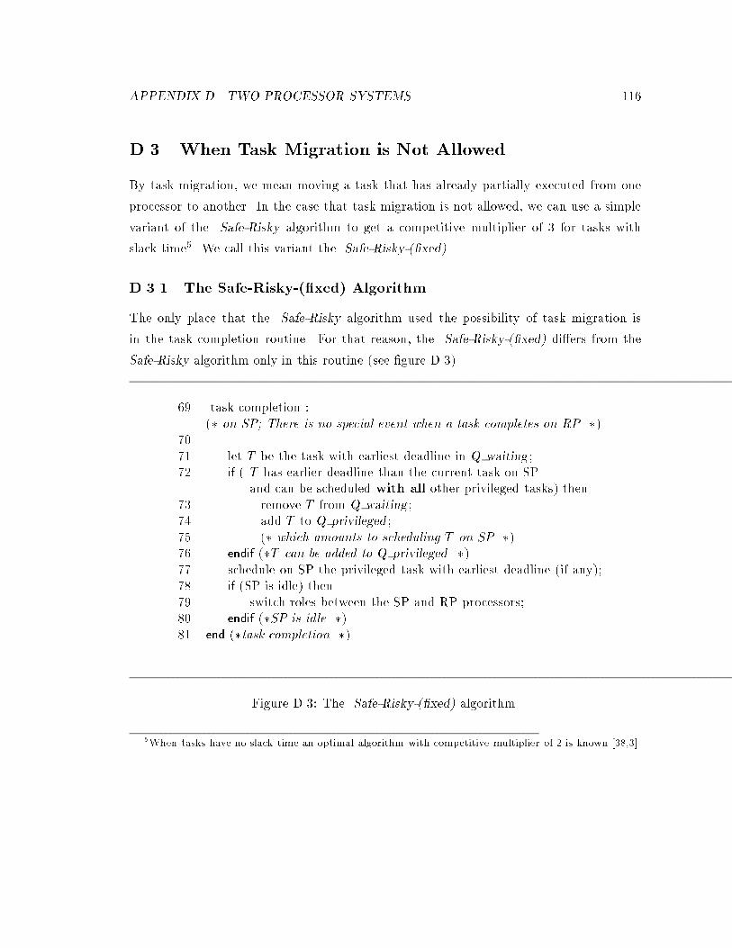
APPENDIX D. TWO PROCESSOR SYSTEMS 116
D.3 When Task Migration is Not Allowed
By task migration, we mean moving a task that has already partially executed from one
processor to another. In the case that task migration is not allowed, we can use a simple
variant of the Safe-Risky algorithm to get a competitive multiplier of 3 for tasks with
slack time5. We call this variant the Safe-Risky-(�xed).
D.3.1 The Safe-Risky-(�xed) Algorithm
The only place that the Safe-Risky algorithm used the possibility of task migration is
in the task completion routine. For that reason, the Safe-Risky-(�xed) di�ers from the
Safe-Risky algorithm only in this routine (see �gure D.3).
69 task completion :(� on SP; There is no special event when a task completes on RP �)
7071 let T be the task with earliest deadline in Q waiting ;72 if ( T has earlier deadline than the current task on SP
and can be scheduled with all other privileged tasks) then73 remove T from Q waiting ;74 add T to Q privileged ;75 (� which amounts to scheduling T on SP �)76 endif (�T can be added to Q privileged �)77 schedule on SP the privileged task with earliest deadline (if any);78 if (SP is idle) then79 switch roles between the SP and RP processors;80 endif (�SP is idle �)81 end (�task completion �)
Figure D.3: The Safe-Risky-(�xed) algorithm.
5When tasks have no slack time an optimal algorithm with competitive multiplier of 2 is known [38,3].
APPENDIX D. TWO PROCESSOR SYSTEMS 117
D.3.2 Analysis
We de�ne latest a�ected and all the other de�nitions as before. Observe that lemmas D.2.1
and D.2.2 hold for the new algorithm as well.
Recall, that F denotes the set of tasks abandoned by the on-line algorithm
Lemma D.3.1 For every interval, I,
C(F ) � 2V (I)
proof.
All tasks that were abandoned by the Safe-Risky-(�xed) were diverted to RP. Let d be
the maximal deadline among all tasks of F 6. The best the clairvoyant can do, with tasks
of F , is to schedule both processors continuously to get a value of 2d. Lemma D.2.2 shows
that the Safe-Risky-(�xed) gets a value of at least d.
Theorem D.3.2 For a system of uniform value density and 2 processors, the Safe-Risky-
(�xed) achieves a competitive multiplier of 3 (when migration of tasks is not permitted).
proof.
This follows from lemma D.3.1 and lemma D.2.5 (applied to the no migration case) and
the Lost Value Lemma (lemma 4.3.1).
D.4 Scheduling Overhead
In this section we study the cost of executing the scheduling algorithms themselves. What
is the cost of testing whether a newly arriving task7 can be added to Q privileged without
causing overload? This test can be done in a constant number of operations (as in Dover).
Q waiting is a 2-3 tree organized according to Latest Start Time. Hence, inserting and
removing a task from this queue costs O(logM) operations. Where, M is a bound on the
total number of ready tasks at any given moment in Q waiting .
During its lifetime, a task causes exactly one task release event and at most one LST
interrupt. Hence, the scheduling overhead per task is O(logM).
6If there is no such maximal deadline, then the supremum is either �nite or in�nity. If it is �nite a
similar proof will work. If it is in�nity, then the interval is in�nitely long, in which case the value obtained
by the on-line algorithm is in�nity.7With an earlier deadline then all the tasks in Q privileged .
