Outside Options, Coercion, and Wages:Removing the Sugar Coating∗

Christian Dippel† Avner Greif‡ Dan Trefler§

December 14, 2019

Abstract

In economies with a large informal sector firms can increase profits by reducing work-ers’ outside options in that informal sector. We formalize this idea in a simple modelof an agricultural economy with plantation owners who lobby the government toenact coercive policies—e.g., the eviction and incarceration of squatting smallholdfarmers—that reduce the value to working outside the formal sector. Using uniquedata for 14 British West Indies ‘sugar islands’ from 1838 (the year of slave emancipa-tion) until 1913, we examine the impact of plantation owners’ power on wages andcoercion-related incarceration. To gain identification, we utilize exogenous variationin the strength of the plantation system in the different islands over time. Whereplanter power declined we see that incarceration rates dropped, and agriculturalwages rose, accompanied by a decline in formal agricultural employment.

Keywords: Labor Coercion, Economic Development, InstitutionsJEL Codes: F1, F16, N26

∗We are especially indebted to Jim Robinson who, in the initial stages of the project when we were wallowing in case studiesdrawn from disparate times and places, encouraged us to focus on the British Empire and the under-exploited Colonial Blue Bookdata. We are also indebted to Elhanan Helpman for his encouragement in exploring the relationship between international tradeand domestic institutions. We benefited from discussions with Daron Acemoglu, Lee Alston, Quamrul Ashraf, Magda Bisieda, KyleBagwell, Abhijit Banerjee, Stanley Engerman, James Fenske, Murat Iyigun, Sara Lowes, Karthik Muralidharan, Suresh Naidu, LuigiPascali, Diego Puga, Manisha Shah, Shanker Satyanath, Alan Taylor, Duncan Thomas, Vitaly Titov, Francesco Trebbi and seminarparticipants at Boulder, CIFAR, ERWIT, Harvard (PIEP) , LSE, Los Andes Namur, the NBER Development Economics Conference,PSE, Ryerson, Stanford, Toronto (Law Faculty), Toulouse, Western, the World Bank, UBC, UC Davis, and UC San Diego. We thankScott Orr, Nicolas Gendron-Carrier, Jacob Whiton and especially Jake Kantor for fantastic research assistance. A previous version ofthis paper was circulated under the title “The Rents From Trade and Coercive Institutions: Removing the Sugar Coating”†University of California, Los Angeles, and NBER.‡Stanford University and “Institutions, Organizations and Growth Program’, Canadian Institute for Advanced Research, Toronto,

Ontario, M5G 1Z8, Canada.§University of Toronto, NBER and “Institutions, Organizations and Growth Program’, Canadian Institute for Advanced Research,

Toronto, Ontario, M5G 1Z8, Canada.

“The fact that the wage level in the capitalist sector depends upon earnings in the

subsistence sector is of immense political importance, since its effect is that capitalists

have a direct interest in holding down the productivity of the subsistence workers.

Thus the owners of plantations, if they are influential in the government, are often

found engaged in turning the peasants off their lands.” — Lewis (1954)

1 Introduction

Many economists and historians would agree with Acemoglu and Wolitzky’s 2011 assessment

that “the majority of labor transactions throughout much of history and a significant fraction of

such transactions in many developing countries today are coercive”. Indeed, labor coercion is at

the heart of much of the literature on long run development and institutional change (Domar,

1970; Engerman, 1999; Acemoglu, Johnson and Robinson, 2001, 2002; Engerman and Sokoloff,

2002; Greif, 2005; Nunn, 2008; Dell, 2010; Naidu, 2010; Nunn and Wantchekon, 2011; Naidu and

Yuchtman, 2013; Bobonis and Morrow, 2014; Ashraf, Cinnirella, Galor, Gershman and Hornung,

2018; Lowes and Montero, 2018). Despite this, rigorous empirical evidence on labor coercion is

scarce and mostly focused on relating present-day outcomes to historical labor coercion.1

Focusing on the workings of labor coercion rather than its long run consequences, we exploit a

historical setting involving 14 British West Indies sugar colonies from 1838 —the year slaves were

emancipated in the British Empire— to 1913. We are thus studying 14 free labor markets at their

inception. Before 1838, the 14 colonies we study were exceedingly similar. Economically, all were

slave societies and all were completely specialized in sugar cane production. Institutionally, all

had the same political and legal systems inherited from Britain and were dominated by a small

group of white planters. After Emancipation, “the main fact of life in the free West Indies was that

black laborers were unwilling to remain submissive and disciplined cane workers” (Green, 1976,

170). We study how planters over the ensuing 76 years used their influence over the state to enact

coercive policies that kept wages low and secured a steady supply of labor.

In keeping with Lewis’ quote, our focus is on ‘legal coercion’, i.e., the use of the state’s leg-

islative and judicial institutions to manipulate workers’ outside options. This focus is particularly

1Two exceptions are Naidu and Yuchtman (2013) and Bobonis and Morrow (2014), summarized below.

1

pertinent where workers’ wages in the formal sector are determined by outside options generated

in the informal sector. Our paper has two empirical objectives: One, we want to test to what extent

legal coercion was used to lower wages. Two, we study the importance of the planters’ economic

and political influence over the government in shaping legal coercion.

To guide our empirics, we employ a simple model where workers earn a wage w that is equal

to their outside option in the informal sector. Coercion C reduces this outside option, e.g., by

evicting smallholders from their plots. Coercive policies C are set by the government to bene-

fit the planters as in Grossman and Helpman’s ‘Protection for Sale’ framework (1994), and the

government chooses a higher C when planters’ influence is greater.2 Planter influence depends

on the number of plantations on the island (N ), which in turn depends on the extent to which

Caribbean plantations offer higher returns to British investors than returns obtainable elsewhere.

In our model a shrinking plantation sector leads to lower levels of coercive activity which raises

wages: N → C → w. Exogenous factors act as an instrument for N .

The data are collected from the British Colonial Office’s Blue Books: wages wit are reported as

the annual average of the agricultural spot market wage. Cit is measured by incarceration rates

per capita. Nit is measured as the share of sugar in total exports or as the share of all plantation

crops in total exports. Our empirical focus is on within-colony over-time panel variation.

Our hypothesis is that where the plantation system went into decline, Cit decreased and wit

increased relative to other islands. A generalized difference-in-differences strategy robustly bears

this out across a range of different specifications. We instrument forNit using exogenous variation

in the returns to investing in Caribbean plantations relative to investing elsewhere. Across islands,

returns in the Caribbean were lower where smallholders could easily escape work on plantations.

Some colonies had large hinterlands while others had next to none.3 Over time, returns to invest-

ing outside of the Caribbean improved rapidly over the 19th century. As the Empire expanded,

2One may think of planter influence as lobbying capacity but this is not explicitly modelled. Our own view is thatlegal coercion is in practice almost always the result of collective action by an elite that influences the state to regulatecoercive labor laws to their benefit, e.g., to reduce rights-at-work, to harass workers in the informal sector or to limitworker mobility, with the ‘Black Codes’ in the post-Bellum U.S. South being a prominent example. In section 2, wedescribe in detail the practical applications of legal coercion in our context.

3 During slavery, this difference did not matter: Land that was unsuitable for sugar lay uncultivated even if it wasvery fertile. After slavery, the availability of hinterlands became important, eroding Nit by making it easier for freedslaves to evade the plantation system. This basic explanation of the divergent post-Emancipation fortunes of ex-slavesacross the islands figures prominently in the literature on Caribbean history and indeed it was anticipated in the 1830sdebates surrounding Emancipation, see Merivale (1861, 312–317), Engerman (1984, 137), Richardson (1997, 134–135,157–8), and Patterson (2013).

2

opportunities to export British manufactures grew much faster than opportunities in Caribbean

agriculture. and English investors turned their attentions away from the Caribbean. Combin-

ing these exogenous elements, our instrument Oit is the product of the cross-section of islands’

hinterlands and the time-series of English exports to non-Caribbean destinations. In the data, a

higher Oit led to a decline in Nit and Cit and a rise in wages. When we instrument for Nit we get

two-stage least-squares (TSLS) estimates that are highly statistically significant and economically

large: A fifty percent decline in the plantation system—roughly the average over the 76 years we

study—would have increased wages by about fifty percent and reduced incarceration rates by

close to their mean of one in a hundred people. These results hold up under an extensive set of

robustness checks.

We also provide evidence on the mechanisms linking N , C, and w. A causal mediation analysis

shows that three-quarters of the negative effect of the plantation system on wages operated via

measured coercion, prima facie evidence for our hypothesis. To lend support to our assumption

that coercion was ‘legal coercion’ exercised by the government in response to pressure from the

plantation system, we study the effects of an exogenous shock which changed the composition of

the plantation-owning elite, while keeping the size of the plantation sector constant. This shock

strengthened the plantation system’s lobbying power with each island’s government apparatus,

but severed the localized ties between the previous plantation owners and the parochial constab-

ulary and judges. We find that this shock increased coercive legislation, which was set centrally,

but decreased incarceration, which depended on these parochial ties. This evidence suggests that

legal coercion adjusted when the planters’ form of influence changed.

We conclude this introduction with a literature review. The importance of using of the leg-

islative, judicial, and policing powers of the state to reduce the outside options of workers and to

benefit a small elite is emphasized by Lewis (1954) and also in Acemoglu and Robinson’s (2012,

ch. 9) study of Apartheid. In the focus on the manipulation of workers’ outside options, we relate

to Alston and Ferrie’s account of Southern Paternalism (1993). The closest empirical study to ours

is Bobonis and Morrow (2014) who show that coffee price shocks in Puerto Rico in the mid-1800s

led elites to reduce human capital investments so as to depress plantation workers’ outside op-

tions. We also connect to a large literature on labor coercion. This literature is more focused on the

coercion of workers on the job (Chwe, 1990; Basu, 1999; Bloch and Rao, 2002; Naidu and Yucht-

3

man, 2013); however, in a principal-agent framework, there is a complementary between coercing

workers on the job, and reducing their outside options as non-workers (Acemoglu and Wolitzky,

2011).4 In our setting, the latter form of coercion was clearly dominant.

In an interesting counter-point to our findings, Dell and Olken (2019) show that the location

of Dutch colonial sugar plantations on the island of Java had positive long-run effects on local

infrastructure and economic development. This line of research suggests that there are potentially

positive and non-institutional long-run consequences of colonial extraction. Lastly, our focus on

the political consequences of geographic variation in the ability to evade the plantation system

connects us to a broader literature on the institutional consequences of geography; see e.g Enger-

man and Sokoloff (2002); Acemoglu et al. (2002).5

2 History

British West Indies plantations were a source of vast profits for British planters and investors.

These profits were dealt a severe blow by the emancipation of slaves in 1838. Emancipation ini-

tially led to sharply rising wages as freed slaves rejected plantation life in favour of squatting on

abandoned estates or small plots in the hinterland. This ‘flight off the estates’ did not last long.

Within a few years of Emancipation the white planter elite had developed a system of legal co-

ercion over labor that lowered wages and slowed the demise of the plantation system. We now

describe the workings of this system.6

2.1 Legal Coercion Cit

Legal coercion in our setting took three main forms. First, coercion restricted access to land. The

full force of the law was brought to bear on peasants who attempted to squat on abandoned es-

tates or Crown land. Squatting was so rampant that it seriously undermined the ability of planters

to keep peasants on plantations. In Jamaica there were 10,000 squatters by 1844 and this number

probably climbed to 40,000 by the mid-1860s (Eisner, 1961, 215–216). The Colonial Blue Books list4 Lowering wages in the bad state in order to induce effort (i.e. relax workers’ incentive compatibility constraint) is

easier if legal coercion simultaneously prevents the worker from walking away (i.e. relaxes the participation constraint).5 Lastly, we naturally connect to a large literature on the Caribbean’s economic adjustment to Emancipation (Eisner,

1961; Engerman, 1982, 1984).6 See Merivale (1861, 340–341), Engerman (1984, 134 and Table 2) and Riviere (1972, 13). On the ‘flight’ see Hall

(1978, 7), Engerman (1982, 199) and Green (1976, 174–175, 198).

4

the titles of all colonial statutes and a quick perusal shows that every colony repeatedly enacted

and strengthened trespass and vagrancy laws in order to prevent squatting. The salience of the

squatting-incarceration issue is illustrated by Jamaica’s Morant Bay Rebellion, which left 600 dead

and many more imprisoned (Underhill, 1895; Craton, 1988).7 Other examples abound: In Do-

minica, the ‘Queen’s Three Chains’ unrest of 1856 was driven by a dispute over whether several

black families had implicit title to or were squatting on the land they were farming. It was resolved

by the rapid dispatch of troops from nearby Antigua (Honychurch, 1984, 136-138). The ‘Toll Bar

Riot’ and the ‘Florence Hall Riot’ in Jamaica were triggered respectively by objections over limiting

smallholders’ access to water sources, and over the sentencing of squatters for trespassing on an

abandoned estate. See Cundall (1906, 5–12).8 A feature of land conflicts in the post-Emancipation

Caribbean was that they resulted from planters’ attempts to reduce peasant smallholders’ outside

options. Planters were not grabbing the land for themselves. In fact, there was plenty of fallow

plantation land during the period we study. For example, in mid-century Jamaica, less than a

quarter of all land was under cultivation and, even on the active plantations, less than half of the

plantation land was in use. That is, disputes were not over land that could be or ever was used

for plantation crops. See Satchell (1990, chapter 4 and especially, 63-64). Land conflict in our case

was thus different from historical episodes in other parts of the world where planters cultivated

land stolen from peasants. See for example Sanchez, del Pilar Lopez-Uribe and Fazio (2010) on

Colombia’s land conflicts 1850–1925 and Acemoglu and Robinson (2012, ch. 9) on Guatemalan’s

coffee land grabs during the same period.

Second, coercion was manifest in asymmetric terms of employment contracts. If a worker

started employment without a formal contract the laws of many colonies stated that he or she had

implicitly entered into a one-month contract. Failure to work during that month was a ‘breach of

contract’ that resulted in fines or imprisonment (House of Commons Parliamentary Papers, 1839b,

7 By 1865, a number of villages had been established illegally on Crown lands in the hills above Morant Bay. Tensionsran high as the government sought to limit further expansion of these villages. Things came to a head during a trespasscase involving a villager who had been pasturing on an abandoned estate (Underhill, 1895, 59). A crowd gathered atthe courthouse, violence broke out, and then quickly ignited all of Jamaica.

8 Planters also lobbied for a host of restrictions which limited worker access to affordable land with clear legal title.Large tracts of Crown land were kept off the market, made available only at artificially high prices, or sold only inlarge lot sizes, e.g., Craton (1997, 390–393). For example, 83% of Trinidad’s landmass was owned by the Crown, yetwas kept off the market for decades after Emancipation (Sewell, 1861, 103, 106, 133). Also, in many colonies peasantswere prohibited from pooling their resources to buy plantations and bankrupt planters were pressured not to sell tosmallholders (Eisner 1961, 211, Craton 1997, 390).

5

205–206). If in addition to wages a worker also received a cottage and a plot for growing crops,

he or she was obligated to work on the plantation for a full year. The law allowed the planter to

evict a peasant for absenteeism (‘breach of contract’) and threats of eviction were very effective in

forcing peasants back to work.9 Laws additionally allowed planters to burn or confiscate cottages

and crops of evicted peasants.10 The resulting destruction led to retribution by peasants who

could then be sentenced to lengthy imprisonment for ‘malicious injury to property.’

Third, coercion was manifest in a tax system that penalized smallholders. This was most

apparent in the biased taxation of imports. Planters imported flour and rice to feed plantation

workers and these imports competed directly with smallhold crops, making smallholding less

attractive. High tariffs on foodstuffs were therefore “opposed by the estate interests since they

tended to deplete labor reserves by driving workers from plantations to the hinterland, where

they grew ground provisions” (Rogers, 1970, 96). Green (1976, 186) similarly states that there was

much political conflict “over import duties on food, [which] enticed freedmen to abandon estate

labor in favor of the production and sale of provisions.” Property taxation was also biased against

smallholders. A smallholder with five acres could pay higher taxes than a planter with 500 acres.

Not only did such abusive smallhold taxes reduce the returns to smallholding, they also led to

punitive loss of title. For example, Satchell (1990, ch. 4 and Table 4.3) documents that 18,000 acres

of Jamaican smallholds were repossessed after 1869 for failure to pay taxes. Many other discrim-

inatory taxes have been documented, including export taxes that were higher on smallhold crops

than on sugar, e.g., Underhill (1895, xvii). Dookhan (1975, 156) emphasizes the importance of such

regressive taxes, arguing in particular that the 1853 ‘Chateau Belair’ Riots in the Virgin Islands

were caused by a new tax on cattle. In his words, “as cattle rearing was primarily the occupation

of the rural negro population, this tax fell principally on them.”

Legal coercion was a fact of life in the British West Indies. Its role was simple: Reduce the

returns to smallholding so as to encourage peasants to work on the plantations for low wages.

Restated in more theoretical language, legal coercion did not affect plantation workers directly;

rather, it affected them indirectly by reducing their outside options.

9 See House of Commons Parliamentary Papers (1839b, 131, 134–136), Bolland (1981, 595), Dookhan (1975, 130), andBrizan (1984, 128).

10 These laws were repeatedly criticized by the Governor of the Leewards in 1838 on the grounds that they wereinequitable and unconstitutional, e.g., House of Commons Parliamentary Papers (1839b, 61–62).

6

2.2 The Government Apparatus

The three pillars of the law — lawmakers, judges and police — were all controlled by planters.

To gauge their coercive effects, it is useful to apply Acemoglu and Robinson’s (2008) distinction

between officially sanctioned de jure power and unofficially sanctioned de facto power. Planters’

de jure power was exercised primarily through their influence on discriminatory laws passed by

legislators in the islands’ legislative assemblies.11 Planters’ de facto power was exercised primarily

through the selective application of these laws in different locations: rural magistrates did much

of their work on plantations, had little legal training and were frequently former plantation over-

seers (McLewin, 1987, 85–87). Local police were also beholden to planters. The first post-Abolition

laws constituting the police force (‘Police Acts’) stated that rural police were to be appointed by

planters. The Leewards Governor complained that this was unconstitutional, but found it difficult

to pressure planter-dominated legislatures into changing the laws (House of Commons Parliamen-

tary Papers, 1839b, 49).

2.3 Planters’ Relative Political Power Nit

We are interested in the impact of the planter elite’s political power Nit on coercion Cit. The

previous section described Cit. We now describe Nit. Planters’ political power was based on their

economic power relative to the peasantry. Economic power in the Caribbean hinged on exports.

Marshall (1968, 253–254) concludes from his survey of the British West Indies that the period from

roughly 1850 to 1900 was one of “continuing expansion of the number of peasants and, more

important, a marked shift by the peasants to export crop production.” This growing peasant

participation in exports was clearly accompanied by the declining acreage of plantations, and the

rising number of freeholders and squatters (Riviere, 1972, 15-17). Eisner (1961, 235) argues that

the “increasing prosperity of the peasantry is thus seen to be mainly due to their growing share in

export crops.”12 Our measure of the relative economic power of the plantation system is thus the

11 Carvalho and Dippel (2016) show that planters completely dominated colonial legislatures, especially in the earlyyears of Emancipation.

12Eisner (1961, 220, 221, and 234) has fine-grained data on Jamaican smallholds and peasant exports. Our owncalculations show that between 1850 and 1890 the share of Jamaican exports originating from freeholds and squattersrose spectacularly from 10.4% to 39.0%.

7

share of plantation crops in total exports.13

Sugar is consistently identified with a plantation mode of production and has often been ar-

gued to be detrimental to economic and social development, e.g., Sokoloff and Engerman (2000)

and Easterly (2007).14 In the British West Indies, sugar was also by far and away the dominant

plantation crop, completely eclipsing all other crops such as cotton or coffee. We therefore use the

share of sugar in total exports as one measure of the strength of the planter elite relative to the

peasantry.

Figure 1 displays the lowess-smoothed share of sugar in total exports by colony. It is best to

focus on the two dominant features. First, in 1838 every colony was highly specialized in sugar.

Second, by 1913 there were substantial cross-colony differences in sugar export shares. Colonies

roughly divided into three groups. Five colonies remained heavily involved in sugar for the entire

period (Antigua, Barbados, Guyana, St. Kitts, and Nevis). Four colonies saw sugar decline to less

than half of total exports (St. Lucia, Trinidad, Tobago, and Jamaica). Five colonies exited sugar

entirely by the end of period (Virgin Islands, Grenada, Dominca, St. Vincent, and Montserrat). In

Figure 1 and the econometric analysis below we use lowess-smoothed export shares because we

are interested in capturing long-run changes in the strength of the plantation system rather than

short-run agricultural fluctuations.15

The data displayed in figure 1 was intimately linked to the planter’s power and influence over

government, in particular their success in securing plantation labor at low wages.16 Dookhan

(1977, 11) argues that across the Caribbean, laborer “drift from the estates” was lowest in Antigua,

13 An acreage-based measure would be an appealing alternative, but the data are only sporadically available. In On-line Appendix Table 12 we provide some evidence that acreage-based and export-based measures are highly correlated.

14 Sugar was unequivocally a plantation crop (Engerman, 1983). However, there is not complete consensus in theliterature about the factors that made it so and such a discussion is beyond the scope of this paper. However, weconjecture that three factors are important. (1) The sugar mill was a major capital asset that was beyond the financialreach of all but the richest members of Caribbean society (Marshall, 1996, 73; Lobdell, 1996, 322, 326). (2) Sugar mustbe processed within hours of harvesting so that there was always a sugar mill either on the plantation or nearby. SeeHigman’s (2001, Figure 2.5) map of Jamaican mills. (3) Labor demand during the sugar harvest was physically brutal(e.g., 90-hour work weeks) and conflicted with workers’ needs to harvest their own provision grounds (Higman, 1984,182–183). These factors favoured a system of production that vertically integrated harvesting with milling at a singlelocation (the plantation) and which, in the racialized post-Emancipation period, used coercion rather than overtimepay as an incentive device, i.e., these three factors favoured a plantation system.

15The lowess smoothing faithfully reproduces the annual data. See Online Appendix Figure 1.16 While we do not focus on this, it is worth noting that the evolution of plantations displayed in figure 1 also

correlated tightly with the share of British Whites in the Caribbean at the time. To European observers at the time, theexodus of whites was synonymous with the decline of the plantation system and the decline of the institutions that haduntil then characterized the British West Indies. We discuss this in detail in Online Appendix B. See also Carvalho andDippel (2016).

8

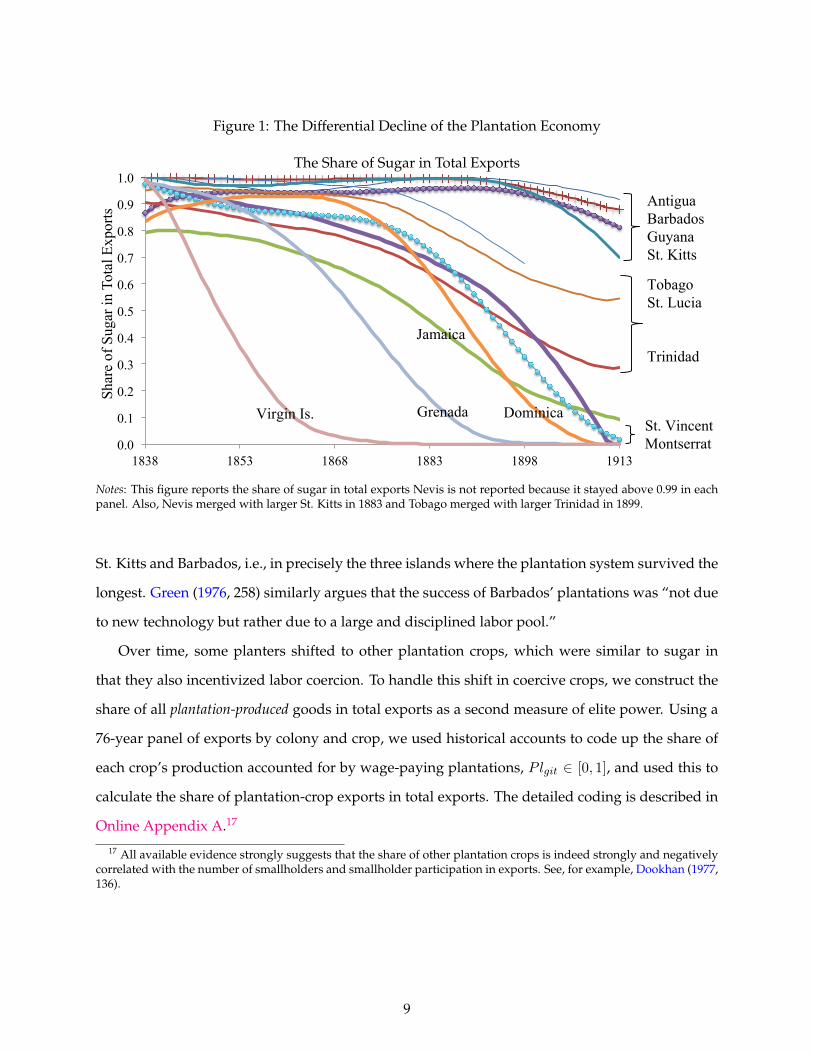
Figure 1: The Differential Decline of the Plantation Economy

The Share of Sugar in Total Exports

0.0

0.1

0.2

0.3

0.4

0.5

0.6

0.7

0.8

0.9

1.0

1838 1853 1868 1883 1898 1913

Shar

e of

Sug

ar in

Tot

al E

xpor

ts Antigua

Barbados Guyana St. Kitts

Tobago St. Lucia Trinidad

St. Vincent Montserrat

Virgin Is.

Grenada Dominica

Jamaica

Notes: This figure reports the share of sugar in total exports Nevis is not reported because it stayed above 0.99 in eachpanel. Also, Nevis merged with larger St. Kitts in 1883 and Tobago merged with larger Trinidad in 1899.

St. Kitts and Barbados, i.e., in precisely the three islands where the plantation system survived the

longest. Green (1976, 258) similarly argues that the success of Barbados’ plantations was “not due

to new technology but rather due to a large and disciplined labor pool.”

Over time, some planters shifted to other plantation crops, which were similar to sugar in

that they also incentivized labor coercion. To handle this shift in coercive crops, we construct the

share of all plantation-produced goods in total exports as a second measure of elite power. Using a

76-year panel of exports by colony and crop, we used historical accounts to code up the share of

each crop’s production accounted for by wage-paying plantations, Plgit ∈ [0, 1], and used this to

calculate the share of plantation-crop exports in total exports. The detailed coding is described in

Online Appendix A.17

17 All available evidence strongly suggests that the share of other plantation crops is indeed strongly and negativelycorrelated with the number of smallholders and smallholder participation in exports. See, for example, Dookhan (1977,136).

9

2.4 Exogenous Drivers of the Strength of the Plantation System

The preceding discussion of Caribbean history suggests regressions of wages and coercion on the

power of the planters. There is naturally a concern that the varying power of the planters dis-

played in Figure 1 was endogenous to factors that may also have affected wages and coercion

directly. It is therefore desirable to identify drivers of Nit that were exogenous in the sense of im-

pacting wages and coercion only throughNit. Our first candidate for such a driver was a source of

cross-sectional variation across colonies that became very salient to peasants after Emancipation.

In a colony like Barbados, all of the land was sugar-suitable and in 1838 only 4% of land was not

under cultivation (1838 Barbados Blue Book). By contrast, a colony like Jamaica had sugar-suitable

coastal plains but a higher-elevation interior (which was fertile but not sugar-suitable). During

slavery this difference between Barbados and Jamaica did not matter because sugar-suitable land

was similarly suitable everywhere and the hinterland was largely inaccessible to slaves and not

used by many others. After Emancipation, differences in the availability of a fertile but sugar-

unsuitable hinterland led to stark differences in the ease with which peasants could evade the

plantation system and resist coercion (Engerman, 1984; Richardson, 1997; Patterson, 2013, respec-

tively 137, 134–135, 157–8).18

To measure this differential ability to evade the planters we carefully calculated the share of

each colony’s land that is unsuitable for sugar cane, Oi.19 The relationship between Oi and the

historical outside options that peasants actually had is visually displayed in Figure 2 for Jamaica,

the only colony with historical maps on evolving land-use patterns. In the left panel, the black

areas are lands that we have coded as highly suitable for sugar cane. In the right panel, the

shaded areas (both black and grey) are plantations in 1790. The two are spatially correlated and,

averaging across Jamaica, the share of land under plantation in 1790 is very close to the share of

highly sugar-suitable land.20 This map and all the post-Emancipation history make clear thatOi is

a good proxy for the amount of hinterlands available to freed slaves after 1838. We note that Oi is

18Engerman (1984, 137) quotes a Jamaican planter in the 1830s as arguing that Emancipation “will be less mischievousto other colonies than ours. For in Barbados and Antigua and several other Islands the liberated slaves must work forwages or want the necessaries of life.”

19We defer data details to section 4 and the appendix sections cited therein.20The right panel of Figure 2 illustrates another point. The grey-shaded areas are plantations that shut down between

1790 and 1890. These were the lands that were most difficult to keep out of peasant hands and were thus a major focusof coercive interventions.

10

Figure 2: Sugar Suitable Land in Jamaica (Left), and Plantations in 1790 and 1890

Notes: The left panel shows the spatial distribution of land that is sugar-suitable (black), only moderately sugar-suitable(dark grey), not sugar-suitable (light grey) and totally sugar-unsuitable (white). See Online Appendix C for details. Theright panel shows the extent of sugar plantations in 1790 (black plus grey areas) and 1890 (black areas). There is a goodmatch between our estimate of sugar-suitable land in the left panel, and the historical sugar plantation land in Jamaica.The left panel is based on authors’ calculations. The right panel is a digitized version of Higman’s (2001) remarkableFigure 2.9.

an extremely good predictor of the long-run survival of the plantation system. This point is made

visually in Online Appendix Figure 7: The higher is Oi, the smaller is the 1913 sugar export share.

In the 18th century British investors made their fortunes in Caribbean sugar. During the 19th

century, however, investment opportunities shifted to other regions. Panel (a) of Figure 3 displays

the per capita GDPs of Britain’s largest export destinations at the start of our sample. Data are

from an update of the Madisson data (Bolt, Inklaar, de Jong and van Zanden, 2018). The only

British West Indies colony with the Madisson data is Jamaica. See the solid line at the bottom of

the panel. The figure shows that while Jamaica languished, the majority of Britain’s largest export

destinations rapidly grew richer.

Exogenous events elsewhere around the globe were overtaking Jamaica and drawing away the

attention of British investors: The repeal of the Corn Laws in 1846 gave a tremendous impetus to

free trade around the world, and started what eventually came to be called the ‘first globalization’,

which, buttressed by a precipitous decline in ocean freight rates, lasted until 1914 (North, 1958;

O’Rourke and Williamson, 2001, 2002).21 In this period, the Caribbean was left behind partly

because the repeal of the Corn included provisions for a phasing-out of preferential tariffs on

West Indies sugar over the period 1846–54 (Curtin, 1954).

This globalization-driven boon and shifting-away of British attention from the Caribbean to-

21 Falling ocean freight rates led to a shift from trade in only high unit-value products like sugar towards trade inmany lower unit value products like heavy machinery exports to the U.S. and Europe.

11

Figure 3: British Markets and British Exports by Destination

(a) per Capita GDP (b) British Exports by Region

020

0040

0060

0080

0010

000

per c

apita

GD

P ($

)

1850 1871 1892 1913

Ausl 2%

USA 12%

Can 6%

Ger 13%

Nld 6%

Fra 5%

Bra 10%

Jam 7%

India 10%

Exports excluding Caribbean

Exports to Caribbean

010

020

030

040

050

0B

ritis

h Ex

ports

(in

1913

£ m

illio

ns)

1838 1853 1868 1883 1898 1913

Notes: Panel (a) is per capita GDP (1990 international dollars) from Madisson, 1850–1913. (Earlier data are not consis-tently available.) The countries included were the top destinations for British exports in 1846 (the earliest date availablefor exports by country) and accounted for 71% of all British exports. The legend reports 1846 export shares, e.g., Ger-many received 13% of all British exports in 1846. Panel (b) is British exports to the Caribbean and British exportsexcluding the Caribbean. These exports are in constant 1913 pounds sterling (£). All exports exclude re-exports.

wards the rest of the world can be seen in export volumes. Panel (b) plots British exports to the

Caribbean and to all non-Caribbean destinations. Data are in constant 1913 pounds sterling (£)

and purged of re-exports (e.g., Jamaican sugar that is shipped first to London and then to France).

The underlying data are from Mitchell (1988) and detailed in Appendix B.5. British exports to

non-Caribbean destinations displays periods of rapid growth followed by shorter periods of stag-

nation (e.g., the 1890s) and infrequent bursts of decline. However, the overall picture is one of

rapid growth, with real exports growing at an annually compounded rate of 3.4%. In compari-

son, British exports to the Caribbean experienced practically no growth. Judged by exports then,

British investors had largely turned their focus away from the Caribbean in response to exoge-

nously improving opportunities elsewhere.

We have focussed on two exogenous drivers of the strength of the plantation system that will

be useful for our identification strategy. Across colonies, coercion on plantations was more difficult

where the hinterland was large. Over time, the plantation system declined in part because British

investors shifted their attention away from Caribbean sugar and towards opportunities in regions

that were experiencing rapid growth.

12

2.5 Other Major Drivers of the Plantation System’s Strength

2.5.1 Crop Price Movements

One challenge for identification is that pressures on the coercive plantation system came in part

from variation in smallhold crop prices. In fact, there was a secular decline in plantation crop

prices relative to smallholder crop prices in the Caribbean during this time.22 Higher smallhold

crop prices would have raised smallhold exports in revenue terms and therefore reduced Nit,

while they would have also increased smallhold profits, and by extension wages, even if planters’

actual power over governance had been unaffected. We therefore carefully control for changes in

the export prices of smallhold crops.23 We also note the importance of inspecting the responses of

Cit to Nit in addition to the wage responses.

We are also concerned with the fact that crop choices were endogenous, irrespective of the

fact that world crop prices were plausibly exogenous to Caribbean production.24 Smallholders’

profits rose more if they substituted towards crops whose prices increased. The impact of the crop

price changes on smallholder profits in turn was biggest in places where the crops with the best

geographic suitability and the steepest price increases coincided. We therefore embed a model of

crop choice into our theory, and include into our empirics an exogenous crop-suitability-driven

export-price basket, estimated as in Costinot, Donaldson and Smith (2016).25

2.5.2 Labor Supply Shocks

Crop prices were not the only factor shaping plantation labor supply during this period. Fortu-

nately, Caribbean history is quite clear on what the other big labor supply shocks were during this

period: the immigration of indentured East Indian Immigrants (Laurence, 1971; Riviere, 1972) and

the construction of the Panama Canal (Maurer and Yu, 2013, ch.4).22This decline in plantation prices, particularly in sugar, was important. A previous version of this paper (Dippel,

Greif and Trefler, 2015) was about the impact of international trade (declining sugar prices) on wages, coercion, andinstitutions. While we continue to carefully control for prices, they are no longer the focus of this paper.

23We additionally control for other important changes in plantation labor supply in the Caribbean during this time,namely the immigration of East Indian laborers and work opportunities from the construction of the Panama Canal.See Appendix B.6.

24World crop prices were exogenous to Caribbean production. Even for sugar, at their production peak in the earlyyears of the data, the British West Indies produced only 18% of world sugar output and this number fell to 1% by theend of the sample. See Online Appendix Figure 4.

25 See Appendix Appendix B.2.

13

2.5.3 Hurricanes

Finally, we note that the Virgin Islands are an outlier in Figure Online Appendix Figure 7: the

plantation system had collapsed by 1913 despite low values of Oi. Nowhere else in the Caribbean

did planter power diminish as rapidly as in the Virgin Islands. See, for example, Online Appendix

Table 1. As it turns out, the Virgin Islands plantation system collapsed because of two major

hurricanes in 1848 and 1852, which destroyed the colony’s sugar infrastructure and left planters

too indebted to rebuild. Hurricanes do two types of damage: They destroy crops and they destroy

structures such as sugar mills. Since sugar cane must be processed within hours of harvesting

and since cane is difficult to transport, there was always a sugar mill either on the plantation

or nearby, e.g., Higman (2001, Figure 2.5). Sugar mills were unique in Caribbean agriculture in

that they were expensive and long-lived assets. They were also prone to hurricane damage. In the

post-Emancipation Caribbean, an increasing share of planters could only cover their variable costs

but not their fixed costs. In other words, it made sense for a marginal planter to operate an existing

mill, but not to rebuild a destroyed mill (Marshall 1996, 73; Lobdell 1996, 322, 326). As a result,

hurricane landfalls that destroyed mills had long-lasting effects. To control for hurricane damage,

we geo-referenced the paths of every major hurricane that hit the Caribbean between 1838 and

1913, and assign each Caribbean hurricane landfall an island-specific damage index HDIit. Data

sources, the list of all hurricanes and their measured impact appear in Online Appendix E.

3 A Simple Model of Coercive Labor Market Institutions

To fix ideas and provide additional motivation for the empirics, we now turn to a simple theory

of coercive labor markets.

3.1 Technology and Crop Choice

There is an exogenous measure L of workers (former slaves) and an endogenous measure N of

planters (members of the planter elite). There is a continuum of heterogeneous plots indexed by

ω, each of which can be planted in one of g = 1, . . . , G crops. We follow Costinot et al. (2016)

in modelling crop choice by assuming that plot ω planted in crop g has a baseline yield of zg(ω)

where zg(ω) is a random variable with a Frechet distribution: Pr{zg(ω) < z} = e−Tgz−θ

. On a

14

plantation, plot ω combined with one worker produces output τpg zg(ω) where τpg ≥ 0 describes

the efficiency of plantation agriculture, e.g., τpg is large for sugar and small for livestock. On a

smallhold, plot ω combined with one worker produces output τ sg zg(ω) where τ sg ≥ 0 describes

the efficiency of smallhold agriculture. The crop-specific τpg and τ sg explain why some crops are

better-suited than others for plantation agriculture.

We consider a small open economy so that crop prices p = (p1, . . . , pG) are exogenous. Crops

are chosen to solve maxg pgτjg zg(ω) where j = p if it is a plantation plot and j = s if it is a smallhold

plot. The optimal choice varies across plots, but on average the expected revenue per plot will be

r(p, τ j) = Emaxgpgτ

jg zg(ω) =

(ΣkTk(τ

jkpk)

θ) 1θ

Γ , j = p, s (1)

where τ j = (τ j1 , . . . , τjG) and Γ = Γ(1/θ − 1) is the gamma function. See Appendix A for the proof

or Costinot et al. (2016, 215). r(p, τ j) captures how crop choices respond to prices.

Each smallholder is randomly allocated one plot and each planter is randomly allocated l(N) ≥

1 plots. Since each plot uses one worker, the maximum number of planters is N = L and when

N = L each planter receives one plot, i.e., l(L) = 1. We also assume that the more planters there

are the more land they receive collectively (∂ ln l(N)N∂ lnN > 0), but not individually (∂ ln l(N)

∂ lnN < 0). The

latter creates a ‘congestion cost’ which ensures that not all agriculture is plantation agriculture.

3.2 The Worker’s Occupational Choice and Coercion

Each smallholder must choose between plantation work and smallholding. Utility from working

on the plantation is w.26 Utility from smallholding is r(p, τ s)− C where C is the negative impact

of planters’ legal coercion on the returns to smallholding. C is endogenous. It follows that in any

equilibrium with both plantation and smallhold agriculture,

w = r(p, τ s)− C . (2)

r(p, τ s) captures how wages respond to prices when crop choices are endogenous.

The costs of coercion (e.g., building jails) are given by Cγ where γ > 1. These costs are funded

26By equating utility with income we are implicitly assuming that only the numeraire good is consumed and that allother goods are exported.

15

by a head tax on planters of Cγ/N . Consider planter profits. When there are N planters, each

receives l(N) plots, earns per plot revenues of r(p, τp), pays per plot wages of r(p, τ s)− C and is

left with profits of

π(C,N) = l(N) [r(p, τp)− r(p, τ s) + C]− Cγ/N . (3)

We use Grossman and Helpman’s (1994) ‘Protection for Sale’ framework to determine the level

of coercion C. C ≥ 0 is chosen to maximize a weighted sum of the profits of the N planters and

the L workers:

W (C) = αNπ + Lw . (4)

α is the weight given to planters’ profits. Our key assumption is that α > 1 so that planters have

greater sway over the choice of coercion. Substituting equations (2)–(3) into (4) and maximizing

with respect to C subject to C ≥ 0 yields the following characterization of optimal coercion. Let N

be the value ofN for which αl(N)N−L = 0. Under our assumptions, N is unique and 0 < N < L.

The optimal level of coercion is

C∗(N) =

(αl(N)N − L

αγ

) 1γ−1

for N ≥ N (5)

and C∗(N) = 0 for N < N . Since the land controlled by planters is increasing in the number of

planters [l(N)N is increasing in N ], equation (5) implies one of our key results, namely, C∗N > 0

when N is sufficiently large. The insight is simple: The stronger is the planter elite, the greater is

its political influence (as measured by αN ) and hence the higher is the level of coercion. Equation

(5) further implies a threshold effect: When the number of planters drops below N , there is no

coercion. See Appendix A for proofs.27,28

27We note in passing that if α = 1 then N = L so that C∗ = 0 for all N , which reflects the fact that coercion is aninefficient redistributive policy that would never be used if smallholders had equal say in choosing coercion.

28This ‘Protection for Sale’ setup abstracts away from part of the collective action problem in that the level of coerciongrows with the number of planters. However, planters do not solve the bigger collective action problem, namely, that ofcollectively restricting entry into planting and thereby preventing profits from being driven to zero. Historically, in themedian colony whites represented only 1.6% of the population so that, in the highly racialized colonial society, whites‘stuck together.’ Thus empirically, there was no white collective action problem when it came to policies restrictingblack smallholders.

16

3.3 Worker Resistance and the Planter’s Entry Decision

As discussed in the history section, workers often resisted white rule, which resulted in deaths,

property damage and incarceration. Since worker motivations for resistance do not enter into

the empirics we model resistance simply as a probability χ that resistance is successful. χ(O) is

increasing in the share of non-sugar-suitable land O because it is costly for the police and military

to operate in these more remote and often highland areas.29 Without loss of generality we assume

χ(O) = O. If resistance is successful neither planters nor workers are able to plant their crops

and returns to each are normalized to 0. If resistance is unsuccessful then workers and planters

generate the earnings, profits, and coercion levels that appear in equations (2)–(5).

We next turn to the free entry condition for planters. Each potential planter must choose be-

tween (1) staying in England where he can invest, export to non-Caribbean countries and earn W

versus (2) moving to the colony where he can invest in sugar, export back to England and earn

planter profits. Conditional on no resistance, planter profits are given by equation (3), namely,

π(N) ≡ π(C∗(N), N). Thus, in the colony the planter earns expected profits (1 − O)π(N). If

(1 − O)π(N) < W for all N then no planter moves to the colony and there is only smallholding.

If (1− O)π(N) > W for all N then L planters move, each has one plot and one worker, and there

are no smallholders. We focus on the intermediate case where planters and smallholders coexist.

In that case there is an N∗ such that (1−O)π(N∗) = W or

π(N∗) =W

1−O . (6)

This equation pins down the equilibrium number of planters N∗. In Appendix A we provide

sufficient conditions on the underlying parameters of the model for such an N∗ to exist and to be

stable in the usual sense that πN (N∗) < 0.

In any stable equilibrium,N∗ is decreasing inO andW . Further,N∗ depends on the interaction

of O with W . We exploit this interaction in the empirical work.30

29The classic example is the 18th century Maroons operating in the mountainous interior of Jamaica.30 From equation (6), ∂N∗/∂W = πN (N∗)/(1 − O) < 0 because πN (N∗) < 0. Likewise, ∂N∗/∂O < 0. While we

do not need to sign ∂2N∗/(∂O∂W ), note that if π(N∗) is linear in N in the neighbourhood of N∗ then an increase in Oincreases ∂N∗/∂W = πN (N∗)/(1 −O), i.e., a higher probability of revolt makes N∗ more sensitive to the returns fromstaying in England.

17

3.4 General Equilibrium and Comparative Statics

An equilibrium in our small open economy is a crop choice for each plot ω and mode j = p, s

that solves maxg pgτjg zg(ω), a wage w that leaves each smallholder indifferent between plantation

work and smallholding (equation 2), a level of coercion C∗(N∗) that maximizes planter-biased so-

cietal welfare (equation 5), and a mass of planters N∗ that leaves each planter indifferent between

staying in England and moving to the colony (equation 6).

Our main comparative statics results are as follows. First, the wage is increasing in an index of

prices r(p, τ s) and decreasing in coercion C. See equation (2). Second, coercion is increasing in the

number of planters. See equation (5). Third, in the absence of coercion, wages are given by w =

r(p, τ s) (equation 2) so that we have a benchmark for competitive wages that deals explicitly with

the crop substitution problem identified in section 2.5.1. Fourth, planter strength N∗ is decreasing

in W/(1−O) and W/(1−O) has no direct impact on anything but N∗.31

4 The Evidence

Our main hypothesis is that the powerful Caribbean planter elite held enough sway over govern-

ment to institute forms of legal coercion such as the incarceration of squatters, which were aimed

at reducing wages. We begin by testing this hypothesis in OLS regressions of coercion (Cit) and

wages (wit) on the relative economic power of the planters (Nit):

wit = βwN ·Nit + γwX ·Xit + λwi + λwt + εwit; (7)

Cit = βCN ·Nit + γCX ·Xit + λCi + λCt + εCit, (8)

where λi are colony fixed effects, λt are year fixed effects or year trends, and Xit are controls.

Data: Our wage data comes from the Blue Books, which report wages for ‘praedial’ or agri-

cultural workers. This was the wage paid to plantation workers. These wages were the largest

component of the cost of the most important economic activity in the colonies (sugar). It is thus

not surprising that wages were a constant subject of discussion in contemporary sources. The Blue

31One could extend the model to include a market for plantation land. We have abstracted from this because landprices are not even remotely consistently available over time or across colonies.

18

Book wage data are identical to the sporadic data from reliable sources discussing wages for sugar

cultivation (e.g., West India Royal Commission, 1897, 107). Further, the Blue Books themselves are

sometimes the source of data quoted by contemporaries (e.g., Sewell, 1861). In short, the Blue Books

reliably reported the well-known and very public data on wages for plantation work. Appendix

B.1 discusses wages at greater length.32, 33

Our coercion data are incarceration rates per capita from the Blue Books. The Books report

the daily average number of prisoners, averaged over the year, for 1838–1913. These data contain

incarcerations for all reasons, but as discussed below and in Appendix B.3 our best estimate is that

two-thirds of incarcerations at the start of our period were associated with legal coercion.34 New

incarcerations per capita (expressed as a percent) had a sample mean of 1.1%, indicating that 1.1%

of the population entered jail each year. Incarceration rates are admittedly a fairly narrow measure

of what was in reality a bundle of policies of legal coercion. The reason we focus on incarceration

rates is that it is the only empirical counterpart to legal coercion that we could consistently code

for the entirety of our wage sample. In the later years we are able to validate this measure using

data on court sentencing that targeted smallholders. See appendix Appendix B.3.

In equations (7)–(8), Xit are controls for observable factors that may have directly affected

wages. Smallholder returns, and therefore plantations wages, were a function of exogenous

price shocks and islands’ crop-specific soil productivity; see the wage equation (2). To construct

ri(pt, τs), we used the Blue Books to construct a 76-year panel of exports by colony and crop—

generating a database containing exports by colony and year for 17 products accounting for 98%

of exports—and combined it with fine-grained information on islands’ agro-climactic conditions

to develop suitability indexes for the most important crops. We then estimated a Frechet-based

structural model of crop choice, as in Costinot et al. (2016), to recover estimates of the ri(pt, τs).

ri(pt, τs) is an index of smallholder revenue based on exogenous crop suitability and it captures

endogenous crop-switching in response to changes in the relative price of crops. It is an exoge-

nous, model-based prediction. See Appendix B.2 for details.

32We work with nominal wages. The Blue Books report that the major components of the cost of living were largelyimported from Britain (clothing and many staples such as flour and rice) so that all 14 colonies shared a common costof living. It follows that the cost of living deflator is absorbed in the year fixed effects used in our regressions.

33Over 90% of the wage data are for a daily pay period and do not involve in-kind payments. Nevertheless, in OnlineAppendix Table 7 we show that our results are not sensitive to adjustments for pay periods or in-kind payments.

34Brizan (1984, 134) arrives at a similar number for Grenada, 1850–1870.

19

Also included in Xit are the major labor-supply shocks discussed in section 2.5.2. For this,

we calculated the island-specific cumulative stock of East Indian immigrant arrivals over time.

It turns out that this flow of migrants was heavily right-skewed. It only really affected Guyana,

Trinidad, and to a lesser extent Jamaica. For the Panama Canal shock, there are no destination-

specific estimates of islands out-migration so we measure the shock with a time-dummy for the

years of Canal construction (1881-1889 under the French and 1908–1913 under the Americans)

divided by distance from island centroids to Panama. See Appendix B.6 for details.

We control for colony size using the log of population and the log of total export revenues.

We control for each colony’s time-varying British support using the number of times the colony is

discussed in the British Parliament.35

OLS Results: Table 1 reports OLS estimates of equations (7) and (8), i.e., the effects of Nit on

wit and Cit. Nit is measured as sugar’s share of exports. Columns 1–4 show results with wit as

the outcome. As a baseline, column 1 includes only a linear and quadratic time trend, and the

Frechet-based index of smallholder export prices ri(pt, τ s). Consistent with the wage equation (2)

in the model, we see that smallholder export prices positively impact wages. In column 2 we add

the controls for Indian immigration and the construction of the Panama Canal, i.e., the two most

important labor supply shocks in the Caribbean during this period. As expected, Indian immi-

gration reduced wages in the islands.36 Proximity to the Panama Canal during the period of its

construction had a positive but insignificant effect on wages. Column 3 additionally controls for

factors that are likely endogenous: As expected, population growth lowered wages and higher

economic activity raised wages. However, their inclusion does not affect the relationship between

wages and Nit. The negative coefficient on the Hansard indicates that declines in Parliamentary

discussions of a colony correlate with declines in the colony’s wage. This is useful because it rules

out a potential source of reverse causality: As a colony’s wage rose, sugar became unprofitable,

Britain lost interest in the colony and stopped subsidizing its white planter elite, and so Nit fell.

That is, the Hansard result is not compatible with wit causing Nit through a British subsidy chan-

nel.35Data are from the Parliamentary Hansard and are available at https://hansard.parliament.uk/search.36The effect of immigration was statistically significant and economically large, but it only really affected two

colonies. It depressed wages by 0.31 log points in Guyana (−0.028 × ln(230, 000)) and by about 0.15 log points inTrinidad.

20

Table 1: OLS Effect of the Plantation System (Nit) on Wages (wit) and Coercion (Cit)

Outcome w it : log wage C it : Incarceration (per Cap.)

(1) (2) (3) (4) (5) (6) (7) (8) (9) (10)

N it : Sugar Exports as -0.3667 -0.3633 -0.3613 -0.3831 -0.3804 0.4459 0.4577 0.4918 0.4183 0.4467

Share of Total Exports [0.0067] [0.0077] [0.0116] [0.0080] [0.0119] [0.0318] [0.0258] [0.0273] [0.0321] [0.0299]

{0.017} {0.029} {0.017} {0.02} {0.017} {0.077} {0.063} {0.079} {0.071} {0.058}

Frechet Smallholder Export 0.3256 0.3263 0.2578 0.1608 0.2149 0.2657 Price Indexit [0.0026] [0.0032] [0.0272] [0.2841] [0.1554] [0.1440]

log (Net Immigration)it -0.0266 -0.0244 -0.0224 -0.0179 -0.0013 -0.0099 0.0065 -0.0009

[0.0023] [0.0017] [0.0110] [0.0146] [0.9325] [0.6680] [0.7071] [0.9705]

log(1/[Dist to Panama])i * 0.0040 0.0036 0.0265 0.0352 -0.0185 -0.0184 0.3637 0.3860

D(1881-1889)|(1908-1913)t [0.3439] [0.4229] [0.6995] [0.5619] [0.0780] [0.0865] [0.0569] [0.0453]

log(Population)it -0.1197 -0.1381 0.1940 0.1412

[0.2864] [0.1480] [0.3893] [0.5839]

log(Value Total Exports)it 0.0716 0.0524 -0.0202 0.0185

[0.0628] [0.2298] [0.8467] [0.8569]

log Hansard-mentionsit 0.0019 0.0096 0.0076 -0.0157

[0.7089] [0.1592] [0.6690] [0.4407]

Time Controls t + t2 t + t2 t + t2t-fe t-fe t + t2 t + t2 t + t2

t-fe t-fe

Observations 908 908 908 908 908 798 798 798 798 798

R-squared 0.711 0.724 0.728 0.768 0.771 0.511 0.516 0.518 0.572 0.574

Notes: Column 1 includes a quadratic time trend and the Frechet-based index of smallholder export prices ri(pt, τs).Column 2 adds the most important labor supply shocks in the Caribbean during this period. Column 3 additionallycontrols for the log of population (a proxy for size), the log of total exports (a proxy for economic size), and Parlia-mentary Hansard mentions (a proxy for British interest in the colony). Column 4 replaces the quadratic time trendwith year fixed effects, and drops the export price index. Column 5 adds the same controls as column 3. In columns6–10, we repeat the same specifications for incarceration as the outcome. Standard errors are clustered by colony andthe corresponding p-values are in square brackets. For the main regressor of interest, p-values for wild-bootstrappedstandard errors are shown in braces.

21

In column 4 we use year fixed effects instead of the quadratic time trend. With year fixed

effects the export price index is never close to significant. We therefore do not include it in any

regressions with year fixed effects. This is done for expositional clarity and its exclusion has no

bearing whatsoever on any of the other coefficients. Column 5 again adds the endogenous con-

trols. Summarizing columns 1–5, the partial correlation between changes Nit and wages is highly

significant, very stable and appears economically large. The estimate βwN in column 4 says that in

a colony like Grenada where sugar’s share in exports had been reduced to zero by the end of the

period, wages had increased by about 38% more over the 76 years than in a colony like Barbados

where sugar’s share in exports remained close to one at the end of the period.

The reader may worry about inference: We always cluster standard errors at the colony level,

as this is intuitively appealing for our panel setting. However, with only 14 clusters we are nat-

urally concerned about the asymptotic theory underlying standard clustering approaches (Moul-

ton, 1986). For our core causal coefficients, we therefore also bootstrap standard errors using the

wild bootstrap, e.g. Cameron and Miller (2008); Davidson and MacKinnon (2010). Throughout

the paper we report p-values for standard errors clustered by colony on all coefficients, and for

our core regressors of interest additionally report those for the wild bootstrap in braces.

In columns 6–10, we repeat these specifications for Cit as the outcome. The resulting estimates

suggest that a complete collapse of the plantation system (from 1 to 0) is associated with a decrease

in incarceration rates of about one person per two-hundred in a year, roughly one half the mean

incarceration rate in the data.37 Consistent with the model, the labour-supply (wage) controls

have no direct effect on coercion. Only the Panama canal control is significant, but switches signs

across specifications. Our model, our intuition and our regression results all tell us that labor

supply shocks do not effect incarceration.

In the remainder of the paper, we estimate all results with two core specifications. The first

corresponds to columns 2 and 7. The second corresponds to columns 4 and 9. That is, we include

either a quadratic time trend or year fixed effects, but omit the potentially endogenous controls

for population, total exports and the Hansard. (Including these endogenous controls alters none

of the results.)

In Table 2 we report the corresponding coefficients on Nit where Nit is now measured as plan-

37To put this number in context, in the United States in 2016, the stock of incarcerated was 0.7 persons per hundred.

22

Table 2: OLS Effect of Sugar-Plantations on Wages (wit) and Coercion (Cit)

Outcome w it : log wage C it : Incarceration (per Cap.)

(1) (2) (3) (4) (5) (6) (7) (8) (9) (10)

N it : Plantation Exports as -0.5076 -0.5131 -0.5084 -0.5504 -0.5391 0.6923 0.6971 0.6963 0.6451 0.6458

Share of Total Exports [0.0030][0.0026][0.0033] [0.0028] [0.0037] [0.0140][0.0148][0.0148] [0.0184] [0.0161]

{0.018} {0.031} {0.018} {0.025} {0.026} {0.02} {0.017} {0.02} {0.028} {0.03}

Time Controls t + t2 t + t2 t + t2t-fe t-fe t + t2 t + t2 t + t2

t-fe t-fe

Observations 908 908 908 908 908 798 798 798 798 798

R-squared 0.717 0.730 0.734 0.776 0.778 0.518 0.522 0.523 0.578 0.578

Notes: This table replicates Table 1 with Nit instead measured as plantation crops’ export share.

tation crops’ export share. The results are similarly robust and stable in magnitude. Across the

board, the coefficients in Panel B are about one third larger than in Panel A, but the economic effect

is almost the same because sugar’s share in exports dropped less than the share of all plantation

crops combined. The estimate βwN in column 4 says that in a colony like Grenada where plantation

crops’ share in exports had been reduced to about one-quarter by the end of the period, wages

had increased by about 38% (0.55 × 0.75) more over the 76 years than in a colony like Barbados

where the plantation system continued to completely dominate.

Endogeneity of Nit aside, the reader may have a number of concerns with Tables 1 and 2. One

potential concern pertains to the claim (and in the model, our assumption) that agricultural wages

are only paid in the plantation sector. We validate this claim in Appendix B.1 where we provide

prima facie evidence that wage employment was the domain of the plantation system, and that the

only common alternative for plantation workers was independent smallhold farming, as opposed

to wage labor outside of agriculture.

Another potential concern pertains to the accuracy of the reported wage data. Wages some-

times included an in-kind component that usually involved a cottage and a small plot. For two-

thirds of our sample the Blue Books indicate whether the wage includes in-kind payments. Only

9% of these observations include in-kind payments. Nevertheless, Online Appendix Table 7 shows

that our results are robust to an adjustment for in-kind payments. Also, wages are almost always

reported as daily, but for 5% of our observations data are reported as weekly or monthly. When

this happens, the Blue Books explicit indicate that the data are for 5-day weeks or 20-day months

23

and so are easily converted to daily wages. Nevertheless, Online Appendix Table 7 shows that our

results are robust to adjustments for alternative conversions of weekly and monthly wages into

daily wages.

Another potential concern pertains to using incarceration rates as our measure of legal coer-

cion. Mitigating this concern is the fact that the historical literature is quite clear that incarceration

was indeed often the result of legal coercion aimed at smallholders. In Appendix B.3 we docu-

ment this by very detailed category of offense for the Leewards for the start of our period. For the

end of our period (1871 to 1913) we have court sentences but only by broad categories of offences,

and only one of these—offences against property—maps into the legal coercion discussed in sec-

tion 2.1. In Appendix B.3 we show that this category’s share of total court sentences correlated

positively with both Nit and Cit.

Identification: The OLS estimates reported thus far should be interpreted with caution because

Nit is likely to be endogenous in both the wage and coercion equations. In the wage equation, for

example, productivity growth in plantation agriculture would have increased both Nit and wit.

Unobserved differential productivity growth would thus bias the OLS results against finding a

negative effect of Nit on wit. In the coercion equation, for another example, if, unobserved to the

econometrician, peasants in some but not all colonies were actively resisting the plantation system

this could have evoked a planter response (increased Cit) while also undermining the plantation

system (decreased Nit).38 This would bias the OLS results against finding a positive effect of Nit

on Cit.

Equation (6) offers a path towards an instrument for Nit. A British investor chooses between

investing in the Caribbean, which returns (1 − Oi)π(Nit), or investing elsewhere, which returns

W t. Across colonies, those colonies exogenously endowed with more hinterlandOi are less likely to

receive the investment. Over time, improvements in non-Caribbean investment opportunities W t

make it less likely that any colony receives the investment. Thus, the larger isOi ·W t the smaller is

Nit.39 We already have a hinterland measure Oi. We also argued in section 2.4 that British exports

38 For instance, Caribbean historiography suggests that the unmeasured proliferation and influence of local mis-sionaries was an important factor that encouraged civil disobedience and undermined the planters; see for exampleDookhan (1977, 156), Lewis (1986, ch.3), McLewin (1987, 85–87), and Holt (1992, ch.7).

39In the model Oi ·W t appears in equation (6), though parameterized slightly differently.

24

to non-Caribbean countries is a good measure of non-Caribbean opportunities W t.40 We expect

that a higher Oi ·W t leads to a lower Nit, i.e., Oi ·W t has a negagtive sign in the first stage.

The Virgin Islands’ experience—where the plantation system collapsed because of two major

hurricanes despite low values of Oi— suggests the need for a second, hurricane-based instrument

HDIit for Nit. (See section 2.5.3.) It is important to be clear about what role HDIit plays: Hurri-

canes are not central to our paper but we need them to fit the variation inNit for the Virgin Islands.

Without the Virgin Islands, hurricanes are no longer needed to fitNit, but we prefer to retain them

in order to reflect the full universe of British Caribbean sugar colonies, and because they were a

particularly striking example of the mechanisms we highlight.

First Stage and Reduced Form Estimation: In moving on to our TSLS estimation, we propose

the following first stage equation

First Stage: Nit = βNO ·Oit + βNH ·HDIit + γNX ·Xit + λNi + λNt + εNit , (9)

as well as the associated reduced form relations

Reduced Form (Wages): wit = βwO ·Oit + βwH ·HDIit + γwX ·Xit + λwi + λwt + εwit; (10)

Reduced Form (Coercion): Cit = βCO ·Oit + βCH ·HDIit + γCX ·Xit + λCi + λCt + εCit, (11)

where i indexes colonies and t indexes years, the λs are fixed effects, and Xit are the same control

variables as in the OLS. Columns 1–4 of Table 3 report estimates of the First Stage equation (9) for

our two favored specifications and for the two different measures of planter power. In columns

1–4, βNO , the coefficient on Oi ·W t indicates that in islands with large hinterlands the plantation

system declined faster in response to improving non-Caribbean opportunities for British interests.

The hurricane damage index HDIit has a powerful negative impact on the plantation system. In

columns 5–8, we report estimates of the two reduced-form equations (10) and (11). The estimate

βwO in column 3 says that compared to Barbados, wages in Grenada (where half the land was

hinterlands) rose substantially more in response to an increase in W t. At the same time, columns

7–8 show a significant effect on incarceration rates working in the opposite direction.

40We include both the British and non-British Caribbean in order to net out Cuba, which produced about a third of

25

Table 3: First Stage and Reduced Form

Outcome N it : Sugar's Export

ShareN it : Plantations'

Export Sharew it : log wage

C it : Incarceration (per Cap.)

(1) (2) (3) (4) (5) (6) (7) (8)

O i x English Exports -0.4819 -0.5238 -0.2365 -0.2611 0.2351 0.2724 -0.4577 -0.4121

to all Non-Caribbeant [0.0000] [0.0001] [0.0012] [0.0030] [0.0153] [0.0075] [0.0056] [0.0287]

{0.002} {0.003} {0.012} {0.008} {0.08} {0.108} {0.02} {0.015}

HDIit -0.0680 -0.0751 -0.0625 -0.0646 0.0483 0.0565 -0.0857 -0.0775

[0.0000] [0.0000] [0.0000] [0.0000] [0.0001] [0.0001] [0.0000] [0.0094]

{0.085} {0.098} {0.067} {0.053} {0.225} {0.114} {0.124} {0.017}

Time Controls t + t2 t-fe t + t2 t-fe t + t2 t-fe t + t2 t-fe

Observations 1,018 1,018 1,018 1,018 908 908 798 798

R-squared 0.853 0.867 0.843 0.851 0.721 0.772 0.526 0.580

Notes: Columns 1–4 present estimates of equation (9), the First Stage relation between the instruments and the twomeasures of Nit. Columns 5–8 present estimates of equations (10) and (11), the Reduced Form relations between theinstruments and the two main outcomes wit and Cit. For each outcome, we present the results for our two preferredspecifications which include a quadratic time trend (odd-numbered columns) or year fixed effects (even-numberedcolumns). These correspond to columns 2 and 4 of Table 1. For brevity, we do not report coefficients on any of thecontrols that appear in Table 1. All specifications include colony fixed effects. Standard errors are clustered by colony,p-values are in square brackets, p-values for wild-bootstrapped standard errors are in braces.

Figure 4: The Year-Specific Effect of Oi on Nit and on wit

-1

0

1

1837 1856 1875 1894 1913Notes: This figure reports the point estimates and 95th-percentile confidence bands on Oit in two estimations ofregression-equations (9) and (10), when Oit is replaced by a flexible interaction of Oi with year fixed effects (whilealso including year fixed effects on their own). The solid thick (red) line reports on the estimated effect on Nit in (9),the solid thin (blue) line reports on the effect on wit in (10); dashed lines are confidence bands.

26

Clearly, the time-varying component of Oit = Oi · W t is a strongly trending variable; see

Panel (b) of Figure 3. Therefore, a potential concern with the results reported in Table 3 is whether

the time path of the effect of Oi on the plantation system and on wages actually matches the

evolution ofW t. The most flexible way to ask this question is to re-estimate equations (9) and (10),

replacing Oit with an interaction between Oi and year fixed effects (while continuing to include

year fixed effects on their own as in columns 2, 4, 6, and 8 of Table 3).

Figure 4 plots the coefficients estimates on this interaction that result from doing so, with 1838

omitted because it gets absorbed by the colony fixed effects as the first year. The solid thick (red)

line shows a clearly discernible negative effect of Oi on Nit, and this effect sets in around the

mid-1860s. The solid thin (blue) line shows a positive effect of Oi on wages kicking in around

the same time.41 We view these time paths as consistent with the time-path of W t, and thus with

our instrument: it is natural that the interaction-effect on Nit in Figure 4 could not drop below −1

since Nit is bounded below at zero; and it is therefore equally natural that the positive effect of Oi

on wit flattens off.

TSLS Estimation: We now turn to the causal effect of the declining strength of the plantation

system on coercion and wages, estimating equations (7) and (8) with TSLS, and using equation (9)

as the first stage for both. Table 4 reports the results for our two preferred specifications. Columns

1–4 report estimates of equations (7) and columns 5–8 report estimates of equation (8). Columns

1–2 and 5–6 report results when Nit is measured as sugar’s share of exports. Columns 3–4 and

7–8 report results when Nit is measured as plantation crops’ share of exports. The estimates βwN

and βCN are very robust in magnitude within pairs of columns (1–2, 3–4 etc.), indicating results do

not hinge on the particular specification of the time controls. The F statistics on the First Stage

instruments are comfortably above critical threshold levels. The TSLS magnitudes βwN in columns

1–2 and 3–4 are about 60% larger than the OLS estimates reported in columns 2 and 4 of Tables

1 and 2. The TSLS magnitudes βCN in columns 5–6 and 7–8 are around twice the OLS estimates

reported in columns 6 and 8 of Tables 1 and 2. In combination, this suggests that the OLS estimates

are downward biased, consistent with the discussion at the start of the identification section.

world sugar cane in our period.41 There is also a temporary spike in wages associated with a cholera epidemic that spread through the Caribbean in

the early 1850s.

27

Table 4: TSLS Effect of the Plantation System (Nit) on Wages (wit) and Coercion (Cit)

Outcome w it : log wage C it : Incarceration (per Cap.)

(1) (2) (3) (4) (5) (6) (7) (8)

N it (Share of Exports) -0.5437 -0.5881 -0.8359 -0.9614 0.7887 0.6354 1.1343 0.9499

[0.0009] [0.0077] [0.0000] [0.0001] [0.0036] [0.0310] [0.0000] [0.0048]{0.005} {0.029} {0.062} {0.037} {0.02} {0.012} {0.036} {0.014}

Frechet Smallholder Export 0.3361 0.3153 0.1870 0.2197 Price Indexit [0.0001] [0.0004] [0.1686] [0.1026]

log (Net Immigration)it -0.0261 -0.0219 -0.0283 -0.0241 -0.0000 0.0073 0.0033 0.0099

[0.0043] [0.0570] [0.0000] [0.0226] [0.9988] [0.7426] [0.8560] [0.6157]

log(1/[Dist to Panama])i x 0.0045 0.0542 0.0038 0.0594 -0.0194 0.3327 -0.0178 0.3593

D(1881-1889) | 1908-1913)t [0.2382] [0.2957] [0.3145] [0.2864] [0.0493] [0.0983] [0.0665] [0.0819]

N it measured based on Sugar Plantations Sugar Plantations

Time Controls t + t2t-fe t + t2

t-fe t + t2t-fe t + t2

t-fe

Observations 908 908 908 908 798 798 798 798

F Statistic (Instruments) 54.8 52.7 9.0 8.4 44.7 51.8 8.1 7.9

Notes: This table reports the TSLS specifications corresponding to the specification in Tables 1 and 2. Columns 1–4report the estimates of the wage equation (7). Columns 5–8 report the estimates of coercion equation (8). In columns1–2 and 5–6, Nit is measured as sugar’s share of exports and plantation crops’ share of exports, respectively. For eachoutcome, we present the results for our two preferred specifications which include a quadratic trend or year fixedeffects. This corresponds to columns 3–4 of Table 1. For expositional clarity, we do not report coefficients on any ofthe controls. All specifications include colony fixed effects. Standard errors are clustered by colony, p-values in squarebrackets. p-values for wild-bootstrapped standard errors are in braces.

28

While we argue that the agro-climactic and international factors that underlie our instrument

Oi · W t have no direct impact on Caribbean wages or coercion, Oi · W t may nevertheless fail

to satisfy the exclusion restriction because it is correlated with omitted variables that influence

wages or coercion. In this section we present a range of specifications which address this concern.

Given the presence of both colony and year fixed effects, the precise concern is that Oi ·W t

is correlated with differential trends across colonies. For concreteness consider the following ex-

ample, chosen because it is particularly damaging to our exclusion restriction. (1) Suppose that

in some colonies labour supply trended up, leading to a fall in wages and a resulting expansion

of sugar (wit ↓→ Nit ↑) while in other colonies labour supply trended down, leading to a rise in

wages and a resulting contraction of sugar (wit ↑→ Nit ↓). (2) Suppose that we have not controlled

for these differential trends in labour supply. (3) Suppose that our instrument is correlated with

these differential trends. Under (1)–(3), our exclusion restriction is violated and a TSLS regression

of wit on Nit would be more negative than the true coefficient. Thus, differential labour supply

trends can potentially explain away our results. In Online Appendix H.1–Online Appendix H.6,

we show that controlling for a variety of different trends leaves the point estimates and signifi-

cance levels of our results qualitatively unchanged.

5 Extensions

In this section, we focus on showing that the negative effect of planter power on wages was in fact

explained by the positive effect of planter power on coercion; and that coercion in our setting was

of the type described in Sections 2.1–2.2.

The history, theory and econometrics presented thus far all point towards the following causal

relations: Oit ↓ → Nit ↓ → Cit ↓ → wit ↑ .However, we have not shown that there is a causal

impact ofCit onwit; we have only shown thatNit impactsCit andwit. To remedy this, we estimate

a model that regresses wit on Cit, and instruments Cit with Oit; reported in Online Appendix I

(Extension I). The model establishes a causal impact of coercion on wages (Cit → wit). This,

however, still does not quantify the relative importance of the politics-coercion mechanism we

postulate (Nit → Cit → wit) because our estimates of the impact of plantation power on wages

(Nit → wit) reported in Section 4 may be capturing our postulated mechanism along with other

29

political mechanisms through which Nit impacts wit. It is therefore of interest to estimate how

much of the impact of Nit on wit operates via coercion as opposed to other political mechanisms.

A decomposition like this is done through a ‘mediation analysis,’ which asks to what extent

the ‘total effect’ of a treatment variable (e.g. Nit) on a ‘final outcome’ (e.g. wit) is explained by

an intermediate outcome or mechanism (e.g. Cit) that is also an outcome of Nit. See for example

Imai, Keele and Yamamoto (2010); Imai, Keele, Tingley and Yamamoto (2011); Heckman, Pinto and

Savelyev (2013); Heckman and Pinto (2015). We use the methodology developed in Pinto, Dippel,

Gold and Heblich (2019) for performing mediation analysis in an IV setting like ours, estimate

that upwards of 75% of the estimated effect of Nit on wit operates through coercion Cit; reported

in Online Appendix I (Extension II).42

One aspect of legal coercion that is emphasized in the historical discussion in Section 2.2 is the

distinction between officially sanctioned de jure power and unofficially sanctioned de facto power.

We now supplement this historical discussion with econometric evidence by investigating the

consequences of the Caribbean Incumbered Estates Act (IEA) of 1854, an exogenous shock to planters’

de facto relative to their de jure power in the exercise of coercion. The IEA originated in the Irish

Potato Famine (1845–1849), which left Irish estate owners without operating capital and deeply

in debt. In response, the Irish Incumbered Estates Act of 1849 strengthened creditor rights by

allowing forced foreclosures (estate sales), which allowed capital to return to the Irish estates. The

success of this legislative innovation, the result of a famine that was exogenous to the British West

Indies, led British Parliament to enact a Caribbean IEA in 1854.43

The most important consequence of the Caribbean IEA was a change in the composition and

identity of the planter elite, because buyers of encumbered estates were often London-based mer-

chant houses rather than local Caribbean planters (Hall, 2011, p.97). This meant that planters with

deep local roots at the parish level were being replaced by London-based merchant houses that

set up offices in colonial capitals, which changed the way legal coercion operated. The de facto

power of the traditional planters elite over local parish police and magistrates made incarceration

42 Results reported in Online Appendix Table 15.43 Before 1838, in the heyday of sugar, many plantations accumulated large encumbrances, that is, financial commit-

ments to pay annual stipends to family members and to repay loans incurred for capital projects such as mills. After1838, rising wages and falling sugar prices led many planters to ignore their encumbrances. They could do so withimpunity because the law subordinated creditors to both the plantation owners and to the London-based merchanthouses who profited from selling sugar. This and the subsequent discussion is based on Cust (1859, p.8–15). Cust wasSecretary to the West Indian Incumbered Estates Commission. See also Hall (2011, p.94–97).

30

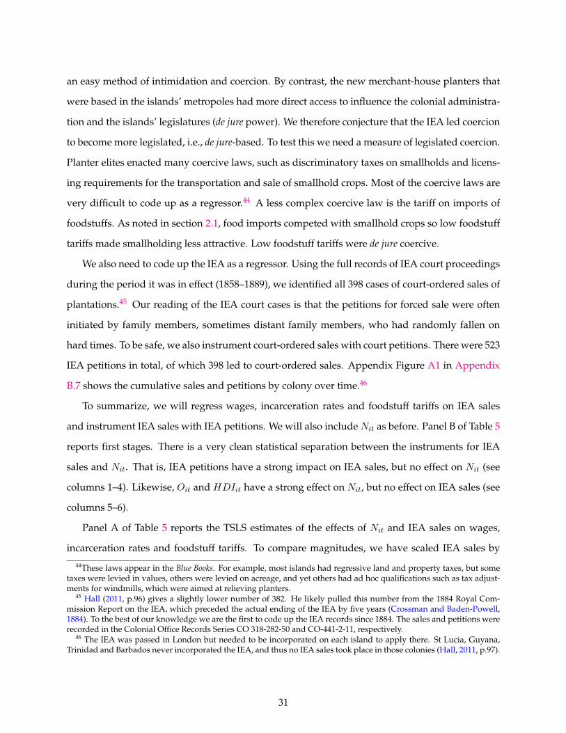
an easy method of intimidation and coercion. By contrast, the new merchant-house planters that

were based in the islands’ metropoles had more direct access to influence the colonial administra-

tion and the islands’ legislatures (de jure power). We therefore conjecture that the IEA led coercion

to become more legislated, i.e., de jure-based. To test this we need a measure of legislated coercion.

Planter elites enacted many coercive laws, such as discriminatory taxes on smallholds and licens-

ing requirements for the transportation and sale of smallhold crops. Most of the coercive laws are

very difficult to code up as a regressor.44 A less complex coercive law is the tariff on imports of

foodstuffs. As noted in section 2.1, food imports competed with smallhold crops so low foodstuff

tariffs made smallholding less attractive. Low foodstuff tariffs were de jure coercive.

We also need to code up the IEA as a regressor. Using the full records of IEA court proceedings

during the period it was in effect (1858–1889), we identified all 398 cases of court-ordered sales of

plantations.45 Our reading of the IEA court cases is that the petitions for forced sale were often

initiated by family members, sometimes distant family members, who had randomly fallen on

hard times. To be safe, we also instrument court-ordered sales with court petitions. There were 523

IEA petitions in total, of which 398 led to court-ordered sales. Appendix Figure A1 in Appendix

B.7 shows the cumulative sales and petitions by colony over time.46

To summarize, we will regress wages, incarceration rates and foodstuff tariffs on IEA sales

and instrument IEA sales with IEA petitions. We will also include Nit as before. Panel B of Table 5

reports first stages. There is a very clean statistical separation between the instruments for IEA

sales and Nit. That is, IEA petitions have a strong impact on IEA sales, but no effect on Nit (see

columns 1–4). Likewise, Oit and HDIit have a strong effect on Nit, but no effect on IEA sales (see

columns 5–6).

Panel A of Table 5 reports the TSLS estimates of the effects of Nit and IEA sales on wages,

incarceration rates and foodstuff tariffs. To compare magnitudes, we have scaled IEA sales by

44These laws appear in the Blue Books. For example, most islands had regressive land and property taxes, but sometaxes were levied in values, others were levied on acreage, and yet others had ad hoc qualifications such as tax adjust-ments for windmills, which were aimed at relieving planters.

45 Hall (2011, p.96) gives a slightly lower number of 382. He likely pulled this number from the 1884 Royal Com-mission Report on the IEA, which preceded the actual ending of the IEA by five years (Crossman and Baden-Powell,1884). To the best of our knowledge we are the first to code up the IEA records since 1884. The sales and petitions wererecorded in the Colonial Office Records Series CO 318-282-50 and CO-441-2-11, respectively.

46 The IEA was passed in London but needed to be incorporated on each island to apply there. St Lucia, Guyana,Trinidad and Barbados never incorporated the IEA, and thus no IEA sales took place in those colonies (Hall, 2011, p.97).

31

Table 5: The Effect of the IEA

Panel A. TSLS Estimation of Effects of Nit and IEA-Salesit on Three Outcomes

Outcome w it : log wage Incarceration (per

Cap.)Import Duties

Flour (£)

(1) (2) (3) (4) (5) (6)

N it : Sugar Exports -0.7151 -0.5683 1.2239 0.9346 -1.0126 -0.6124

Share of Total Exports [0.0004] [0.0181] [0.0001] [0.0031] [0.3102] [0.5148]

IEA Salesit -0.0388 -0.0589 -0.0662 -0.0547 -0.3593 -0.4226

[0.0495] [0.0258] [0.2909] [0.4050] [0.0026] [0.0298]

Time Controls t + t2t-fe t + t2

t-fe t + t2t-fe

Observations 908 908 798 798 942 942

p-value: Test[ 2 coefficients equal] 0.001 0.031 0.000 0.002 0.515 0.835

F Statistic (Instruments) 18.878 15.111 17.581 17.279 21.146 17.397

Panel B. First Stage for Two Endogenous Regressors: Nit and IEA-Salesit

Outcome N it : Plantations'

Export ShareN it : Sugar's Export Share

IEA Salesit

(1) (2) (3) (4) (5) (6)

O i x English Exports -0.2399 -0.2359 -0.4452 -0.4925 0.0517 0.1095

to all Non-Caribbeant [0.0075] [0.0025] [0.0001] [0.0001] [0.5780] [0.3414]

HDIit -0.0665 -0.0665 -0.0677 -0.0718 0.0076 0.0140

[0.0000] [0.0000] [0.0000] [0.0000] [0.3717] [0.2126]

Incumbered Estate Act (IEA) -0.0227 -0.0214 -0.0133 -0.0177 1.0367 1.0522

Petitionsit [0.1734] [0.2438] [0.5498] [0.4786] [0.0000] [0.0000]

Time Controls t + t2t-fe t + t2

t-fe t + t2t-fe

Observations 1,018 1,018 1,018 1,018 1,018 1,018

R-squared 0.882 0.884 0.891 0.897 0.991 0.990Notes: (a) Panel A presents the TSLS Estimation of the effect on three outcomes. Online Appendix Table 16 reportsadditional robustness checks on Panel A. Panel B presents the First Stage Results for two endogenous regressors, i.e.,Nit and IEA-Salesit. Because there are 3 different numbers of observations in Panel A, we report the First Stage in PanelB for all available data. In Online Appendix Table 17, we also report the First Stage for each of the 3 sets of observationsin Panel A. This does not materially affect any coefficients. (b) For each outcome, we present the results for our twopreferred specifications, i.e., the second and third specifications shown in all results in section 4. (c) Standard errors areclustered by colony, p-values in square brackets.

32

their mean.47 The coefficients on IEA sales are thus the average effect of the IEA. The effects of Nit

on wages and incarceration rates (columns 1–4) are almost identical to our baseline Table 4 results.

The average total impact of the IEA on wages was to lower them by approximately 5.89 percent

(in column 2). In contrast, Nit declined on average by 0.5 and so lowered wages by approximately

28.4 percent (= 0.5× 0.568). This suggests that the collapse of the plantation system (Nit) was the

much more fundamental shock to labor markets than the introduction of the IEA, which is fully

consistent with the historical literature. This eyeball observation is also borne out in a statistical

test of the equality of the two coefficients of interest (on Nit and on IEA sales), which we report at

the bottom of Panel A. When it comes to incarceration, the effect of IEA sales was not only much

smaller than that of Nit but was in fact statistically not distinguishable from zero (in columns

3–4). This stands in contrast to the effects on foodstuff tariffs, where columns 5–6 show that as

the plantation system weakened (Nit fell), foodstuff tariffs rose to the benefit of smallholders, but

that this effect is statistically insignificant.48 In contrast, and as hypothesized, columns 5–6 also

show the higher de jure access of the new merchant-planters brought in by the IEA to the islands’

lawmakers led to a much more precisely estimated reduction in foodstuff tariffs.49

In summary, the IEA sales provide evidence on the use of de facto versus de jure coercion. IEA

sales did not increase de facto coercion as measured by incarceration rates (the results in columns

3–4 are insignificant), did increase de jure coercion as measured by lower foodstuff tariffs. The

shape of legal coercion in the British West Indies varied with changes in the political power of the

planter elite.

6 Conclusion

In this paper, we provide the first rigorous empirical evidence on the importance of legal coercion

in informal developing-country labor markets. Following Lewis’ famous assessment quoted at the

beginning of this paper, we hypothesize that legal coercion aimed at depressing workers’ outside

47 In the full panel data, the average observation (over time and across all islands with any sales) had a cumulativenumber of IEA sales of 28. See Figure A1.

48 We do not report wild bootstrap standard errors, which blow up when instrumenting two endogenous variables.49 Seeing as the point estimates of the effect of Nit on foodstuff tariffs are imprecise but large, we do not have the

statistical power to reject that the effects of Nit and IEA-Salesit on tariffs are equal. In Online Appendix Table 16 wereport additional specifications where we control for general changes in public finance (revenues and expenditures) inour data.

33

options in the informal sector is an important factor in determining wages, and that the formal

sector’s influence over government is a key driver of the use of legal coercion.

We focus on a uniquely relevant empirical setting, studying 14 Caribbean plantation islands

at the inception of free labor markets, i.e., starting right after the Emancipation of slaves. We

measure the formal sector’s influence over government Nit by the plantation sector’s share of

overall production. To gain identification, we instrument for Nit with a interaction between the

planters’ time-varying reservation wages outside the Caribbean plantation system and variation

across islands in the peasants’ ability to evade the plantation system.

Controlling for possibly confounding crop price variation, labor demand and labor supply

shocks, we find strong support for both hypotheses in the data: The plantation system had pow-

erful effects on wages and legal coercion (see Tables 1 and 4). A complete collapse of the plantation

system raised agricultural wages by 100% and lowered coercion by two times its mean level in the

data. At the sub-island parish-level we can also show that it lowered mortality rates. Pushing

further towards identifying the causal mechanism linking these patterns, we find that upwards

of three-quarters of the plantation system’s effect on wages is explained by the plantation sys-

tem’s effect on coercion (see Online Appendix Table 15). We also provide suggestive evidence that

planters shaped legal coercion both through legislation passed in the islands as well as through

personal connections to the police and judicial apparatus in the countryside.

In summary, Lewis was right.

References

Acemoglu, Daron and Alexander Wolitzky, “The Economics of Labor Coercion,” Econometrica,2011, 79 (2), 555–600.

and James A. Robinson, “Persistence of Power, Elites, and Institutions,” American EconomicReview, March 2008, 98 (1), 267–293.

and , Why Nations Fail: The Origins of Power, Prosperity, and Poverty, New York, NY: CrownPublishing, 2012.

, Simon Johnson, and James A. Robinson, “The Colonial Origins of Comparative Develop-ment: An Empirical Investigation,” The American Economic Review, 2001.

, , and , “Reversal of Fortune: Geography and Institutions in the Making of the ModernWorld Income Distribution,” The Quarterly Journal of Economics, 2002, 117 (4), 1231–1294.

34

Alston, Lee J and Joseph P Ferrie, “Paternalism in Agricultural Labor Contracts in the US South:Implications for the Growth of the Welfare State,” The American Economic Review, 1993, pp. 852–876.

Antras, Pol and Alonso de Gortari, “On the Geography of Global Value Chains,” Working PaperNo. 23456, National Bureau of Economic Research, May 2017.

Ashraf, Quamrul H, Francesco Cinnirella, Oded Galor, Boris Gershman, and Erik Hornung,“Capital-Skill Complementarity and the Emergence of Labor Emancipation,” Technical Report2018.

Basu, Kaushik, “Child Labor: Cause, Consequence, and Cure, with Remarks on InternationalLabor Standards,” Journal of Economic Literature, 1999, 37 (3), 1083–1119.

Blattman, Christopher, Jason Hwang, and Jeffery G. Williamson, “Winners and Losers in theCommodity Lottery: The Impact of Terms of Trade Growth and Volatility in the Periphery 1870-1939,” Journal of Development Economics, 2007, 82 (1), 156–179.

Bloch, Francis and Vijayendra Rao, “Terror as a Bargaining Instrument: A Case Study of DowryViolence in Rural India,” The American Economic Review, 2002, 92 (4), 1029.

Bobonis, Gustavo J. and Peter M. Morrow, “Labor Coercion and the Accumulation of HumanCapital,” Journal of Development Economics, 2014, 108 (0), 32–53.

Bolland, O.Nigel, “Systems of Domination After Slavery: The Control of Land and Labor in theBritish West Indies after 1838,” Comparative Studies in Society and History, 1981, 23 (4), 591–619.

Bolt, Jutta, Robert Inklaar, Herman de Jong, and Jan Luiten van Zanden, “Rebasing ‘Maddison’:New Income Comparisons and the Shape of Long-Run Economic Development,” 2018.

Brizan, George I., Grenada, Island of Conflict: from Amerindians to People’s Revolution, 1498-1979,London: Zed Books, 1984.

Cameron, A Colin and Douglas L Miller, “Bootstrap-Based Improvements for Inference withClustered Errors,” Review of Economics and Statistics, 2008, 90 (3), 414–427.

Carvalho, Jean Paul and Christian Dippel, “Elite Identity and Political Accountability: A Tale ofTen Islands,” Technical Report, NBER Working Paper 22777 2016.

Chwe, Michael Suk-Young, “Why Were Workers Whipped? Pain in a Principal-Agent Model,”The Economic Journal, 1990, 100 (403), 1109–1121.

Costinot, Arnaud, Dave Donaldson, and Cory Smith, “Evolving Comparative Advantage andthe Impact of Climate Change in Agricultural Markets: Evidence from 1.7 Million Fields aroundthe World,” Journal of Political Economy, February 2016, 124 (1), 205–248.

35

Craton, Michael, “Continuity Not Change: The Incidence of Unrest Among Ex-Slaves in theBritish West Indies, 1838–1876,” Slavery and Abolition, 1988, 9 (2), 144–170.

, Empire, Enslavement, and Freedom in the Caribbean, Princeton: Markus Wiener Publishers, 1997.

Crossman, Colonoal C.M.G and George Esq. M.A. Baden-Powell, Report on the West Indian In-cumbered Estate Act, London: Eyre and Spottiswoode, 1884.

Cundall, Frank, Political and Social Disturbances in the West Indies: A Brief Account and Bibliography,London: H. Sotheran & Co., 1906.

Curtin, Philip D., “The British Sugar Duties and West Indian Prosperity,” Journal of EconomicHistory, Spring 1954, 14 (2), 157–164.

Cust, Reginald John Esq., A Treatise on the West Indian Encumbered Estate Acts, London: WilliamAmer, Law Bookseller, 1859.

Davidson, R. and J.G. MacKinnon, “Wild Bootstrap Tests for IV regression,” Journal of Businessand Economic Statistics, 2010, 28 (1), 128–144.

Deerr, Noel, The History of Sugar, London: Chapman and Hall, 1950.

Dell, Melissa, “The Persistent Effects of Peru’s Mining Mita,” Econometrica, November 2010, 78(6), 1863–1903.

and Benjamin A Olken, “The Development Effects of the Extractive Colonial Economy: TheDutch Cultivation System in Java,” The Review of Economic Studies, 03 2019.

Dippel, Christian, Avner Greif, and Daniel Trefler, “The Rents From Trade and Coercive Institu-tions: Removing the Sugar Coating,” NBER Working Paper No. 20958 February 2015.

Domar, Evsey D., “The Causes of Slavery or Serfdom: A Hypothesis,” Journal of Economic History,1970, 30 (1), 18–32.

Dookhan, Isaac, A History of the British Virgin Islands, 1672–1970, Epping, England: CaribbeanUniversities Press, 1975.

Dookhan, Issac, A Post-Emancipation History of the West Indies, Collins, 1977.

Easterly, William, “Inequality does Cause Underdevelopment: Insights from a New Instrument,”Journal of Development Economics, 2007, 84 (2), 755–776.

Eaton, Jonathan and Samuel Kortum, “Technology, Geography, and Trade,” Econometrica,September 2002, 75 (5), 1741–1779.

Eisner, Gisela, Jamaica, 1830-1930: A Study in Economic Growth, Manchester: Manchester Univer-sity Press, 1961.

36

Engerman, Stanley, Terms of Labor: Slavery, Serfdom, and Free Labor, Stanford University Press,1999.

Engerman, Stanley L., “Economic Adjustments to Emancipation in the United States and BritishWest Indies,” Journal of Interdisciplinary History, 1982, 13 (2), 191–220.

, “Contract Labor, Sugar and Technology in the Nineteenth Century,” Journal of Economic History,September 1983, 43 (3), 635—659.

, “Economic Change and Contract Labor in the British Caribbean: The End of Slavery and theAdjustment to Emancipation,” Explorations in Economic History, 1984, 21 (2), 133–150.

and Kenneth L. Sokoloff, “Factor Endowments, Inequality, and Paths of Development AmongNew World Economics,” Technical Report, National Bureau of Economic Research 2002.

Green, William A., British Slave Emancipation: The Sugar Colonies and the Great Experiment 1830-1865, Oxford: Clarendon Press, 1976.

Greif, Avner, “Commitment, Coercion, and Markets: The Nature and Dynamics of InstitutionsSupporting Exchange,” in Claude Menard and Mary M. Shirley, eds., Handbook for New Institu-tional Economics, Norwell, MA: Kluwer Academic Publishers, 2005, pp. 727–788.

Grossman, Gene M. and Elhanan Helpman, “Protection for Sale,” American Economic Review,September 1994, 84 (4), 833–850.

Hall, Douglas, “The Flight From the Estates Reconsidered: The British West Indies 1838–1842,”Journal of Caribbean History, 1978, 10 (11), 7–24.

, “The Crisis of the Plantation,” in K.O. Laurence, ed., General History of the Caribbean Volume 4 -the Long 19th Century, UNESCO Books, 2011.

Heckman, James J and Rodrigo Pinto, “Econometric Mediation Analyses: Identifying the Sourcesof Treatment Effects from Experimentally Estimated Production Technologies with Unmeasuredand Mismeasured Inputs,” Econometric Reviews, 2015, 34 (1-2), 6–31.

Heckman, James J., Rodrigo Pinto, and Peter A. Savelyev, “Understanding the MechanismsThrough Which an Influential Early Childhood Program Boosted Adult Outcomes,” AmericanEconomic Review, 2013, 103 (6), 2052–2086.

Higman, Barry W., Slave Populations of the British Caribbean, 1807–1834, Baltimore: John HopkinsUniversity Press, 1984.

, Jamaica Surveyed: Plantation Maps and Plans of the Eighteenth and Nineteenth Centuries, Mona,Jamaica: University of West Indies Press, 2001.

Holt, Thomas C., The Problem of Freedom: Race, Labor, and Politics in Jamaica and Britain, 1832–1938,Johns Hopkins University Press, 1992.

37

Honychurch, L., The Dominica Story: A History of the Island, Roseau: The Dominica Institute, 1984.

House of Commons Parliamentary Papers, Papers Relative to the West Indies, Part II. The WindwardIslands’ Government, Printed for the House of Commons, March 1839.

, Papers Relative to the West Indies, Part III. Leeward Islands, Printed for the House of Commons,March & August 1839.

Imai, Kosuke, Luke Keele, and Te Yamamoto, “Identification, Inference and Sensitivity Analysisfor Causal Mediation Effects,” Statistical Science, 2010, 25 (1), 51–71.

, , Dustin Tingley, and Teppei Yamamoto, “Unpacking the Black Box of Causality: Learningabout Causal Mechanisms from Experimental and Observational Studies,” American PoliticalScience Review, 2011, 105 (4), 765–789.

Laurence, Keith O., Immigration into the West Indies in the 19th Century, Epping, England:Caribbean Universities Press, 1971.

Lewis, Gordon K., The Growth of the Modern West Indies, New York: Monthly Review Press, 1986.

Lewis, W Arthur, “Economic Development with Unlimited Supplies of Labour,” The ManchesterSchool, 1954, 22 (2), 139–191.

Lobdell, Richard, “Patterns of Investments and Credit in the British West Indian Sugar Industry,1838–1897,” in Hilary Beckles and Verene Shepherd, eds., Caribbean Freedom: Economy and Societyfrom Emancipation to the Present, Princeton: Markus Wiener, 1996, pp. 319–329.

Lowes, Sara and Eduardo Montero, “Concessions, Violence, and Indirect Rule: Evidence fromthe Congo Free State,” 2018.

Marshall, Woodville K., “Notes on Peasant Development in the West Indies since 1838,” Socialand Economic Studies, September 1968, 17 (3), 252–263.

, “Metayage in the Sugar Industry of the British Windward Islands, 1838–1865,” in Hilary Beck-les and Verene Shepherd, eds., Caribbean Freedom: Economy and Society from Emancipation to thePresent, Princeton: Markus Wiener, 1996, pp. 64–79.

Maurer, Noel and Carlos Yu, The Big Ditch: How America Took, Built, Ran, and Ultimately Gave Awaythe Panama Canal, Princeton University Press, 2013.

McLewin, Philip J., Power and Economic Change: The Response to Emancipation in Jamaica and BritishGuiana, 1840-1865, Princeton, NJ: Garland, 1987.

Merivale, Herman, Lectures on Colonization and Colonies, London: Longman, Green and Roberts,1861.

38

Michalopoulos, Stelios, “The Origins of Ethnolinguistic Diversity,” American Economic Review,2012, 102 (4), 1508–1539.

Mitchell, B.R., British Historical Statistics, Cambridge, England: Cambridge University Press, 1988.

Moulton, Brent R, “Random Group Effects and the Precision of Regression Estimates,” Journal ofEconometrics, 1986, 32 (3), 385–397.

Naidu, Suresh, “Recruitment Restrictions and Labor Markets: Evidence from the Postbellum U.S.South,” Journal of Labor Economics, April 2010, 28 (2), 413–445.

and Noam Yuchtman, “Coercive Contract Enforcement: Law and the Labor Market in Nine-teenth Century Industrial Britain,” American Economic Review, 2013, 103 (1), 107–44.

North, Douglass, “Ocean Freight Rates and Economic Development 1730-1913,” The Journal ofEconomic History, 1958, 18 (4), 537–555.

Nunn, Nathan, “The Long Term Effects of Africa’s Slave Trades,” Quarterly Journal of Economics,February 2008, 123 (1), 139–176.

and Leonard Wantchekon, “The Slave Trade and the Origins of Mistrust in Africa,” AmericanEconomic Review, 2011, 101 (7), 3221–3252.

O’Rourke, Kevin H. and Jeffrey G. Williamson, Globalization and History: the Evolution of aNineteenth-Century Atlantic Economy, The MIT Press, 2001.

O’Rourke, Kevin H and Jeffrey G Williamson, “When did Globalisation Begin?,” European Re-view of Economic History, 2002, 6 (1), 23–50.

Paget, Hugh, “The Free Village System in Jamaica,” Caribbean Quarterly, 1964, 10 (1), 38–51.

Patterson, O, “Institutions, Colonialism and Economic Development: the Acemoglu-Johnson-Robinson (AJR) Thesis in Light of the Caribbean Experience,” 2013.

Pinto, R., C. Dippel, R. Gold, and S. Heblich, “Mediation Analysis in IV Settings With a SingleInstrument,” 2019.

Richardson, Bonham C., Economy and Environment in the Caribbean: Barbados and the Windwards inthe Late 1800s, Mona, Jamaica: University of the West Indies Press, 1997.

Riviere, W.Emanuel, “Labour Shortage in the British West Indies after Emancipation,” Journal ofCaribbean History, 1972, 4, 1–30.

Roberts, G.W. and J. Byrne, “Statistics on Indenture and Associated Migration Affecting the WestIndies, 1834–1918,” Population Studies, July 1966, 20 (1), 125–134.

Rogers, Howard Aston, “The Fall of the Old Representative System in the Leeward and Wind-ward Islands, 1854-1877.” PhD dissertation, University of Southern California. 1970.

39

Sanchez, Fabio, Marıa del Pilar Lopez-Uribe, and Antonella Fazio, “Land Conflicts, PropertyRights, and the Rise of the Export Economy in Colombia, 1850–1925,” The Journal of EconomicHistory, 2010, 70 (2), 378–399.

Satchell, Veront M., From Plots to Plantations: Land Transactions in Jamaica, 1866–1900, Mona, Ja-maica: Institute of Social and Economic Research, 1990.

Sewell, William G., The Ordeal of Free Labor in the British West Indies, Harper & brothers, 1861.

Sokoloff, Kenneth L. and Stanley L. Engerman, “History Lessons: Institutions, Factor Endow-ments, and Paths of Development in the New World,” Journal of Economic Perspectives, 2000, 14(3), 217–232.

Underhill, Edward Bean, The Tragedy of Morant Bay: A Narrative of the Disturbances in the Island ofJamaica in 1865, Alexander & Shepheard, 1895.

West India Royal Commission, Report of the West India Royal Commission, New York, NY: Eyre andSpottiswoode, 1897.

40

Appendix A Mathematical Proofs

Proof of Equation (1): Drop j superscripts, i and t subscripts, and pt arguments. Define Tg ≡Tg(τgpg)

θ. Let rg(ω) = Tgzg(ω)θ be revenue per plot generated by crop g. Then rg(ω) has cu-mulative distribution e−Tgr

−θg , density θTge

−Tgr−θ and mean T1/θg Γ(1 − 1/θ). As is well known

from Eaton and Kortum (2002), Pr{rk(ω) < r ∀k 6= g} = e−(T−Tg)r−θ

where T = ΣGk=1Tk

and Pr{choose g} = Tg/T . Hence, the joint probability of g being the optimal crop choice andrg(ω) = r is

Pr{ {choose g} and {rg(ω) = r} } = Pr{rk(ω) < r ∀k 6= g}Pr{rg(ω) = r} = (θT e−T r−θ

)(Tg/T ) .

The first term in parentheses is a Frechet density with scale parameter T and hence with meanT 1/θΓ. Hence the expected revenues generated by crop g are

rg(Tg) ≡ E[rg(ω)] = T 1/θΓ(Tg/T ) = TgT1θ−1Γ . (12)

Further, the expected revenues generated by all crops are

r(Tg) ≡ Σgrg(Tg) = T1θΓ (13)

where T ≡ Σg=1Tg. Substituting Tg ≡ Tg(τgpg)θ into this mean yields equation (1). Q.E.D.

Characterization ofC∗(N): Substituting equations (2)-(3) into (4) yieldsW (C) = (αl(N)N−L)C−αCγ+αl(N)N [r(p, τp)−r(p, τ s)]+Lr(p, τ s), which is concave inC for γ > 1. HenceC∗ is unique.∂W/∂C = 0 implies (C∗)γ−1 = [αl(N)N − L]/[αγ]. From the definition of N before equation (5),αl(N)N − L > 0⇔ N > N . Hence the constrained (C ≥ 0) optimal solution is C∗ = 0 for N < N

and equation (5) for N ≥ N .

Existence, Interior Solutions, and Stability of N∗: The equilibrium number of planters N∗ isgiven by equation (6). We first derive a sufficient condition which ensures an interior solutionN∗ ∈ (0, L). Start by defining ∆r ≡ r(p, τp) − r(p, τ s). A sufficient condition for an interior N∗

is π(0) > W/(1 − O) > π(L). From equation(5), C∗(0) = 0 so that from equation (3), π(0) =

l(0)∆r. Also, it is tedious but straightforward to show that π(L) < ∆rL1/(γ−1). Hence a sufficientcondition on parameters is l(0)∆r > W/(1 − O) > ∆rL1/(γ−1). To see stability, consider a plot ofπ(N) and W/(1−O) against N . As we move from N = 0 to N = L, π(N) must cut the horizontalW/(1− O) line from above, which is the requirement for stability. Finally, at such an intersectionN = N∗ and πN (N∗) < 0.

Appendix B Data

We made use of two types of original data sources. The first is new dataset of geographic andagro-climatic conditions in the Caribbean. To calculate pre-determined outside options as well as

41

Frechet-based structural model of crop choice, we need detailed spatial data on soil suitability fordifferent crops. Standard sources for crop-suitability data are too coarse for our colonies.50 Wetherefore gathered agro-climatic data on the Caribbean at an unusually fine spatial level and thendeveloped agro-climatic suitability indexes for the 8 most important crops in our data.

The second source of novel data is archival. Starting in the mid-1830s, Britain began collectingstatistics on colonial conditions. Each colony filled out an annual Blue Book and sent it to Londonwhere it is now stored in the British National Archives. We photographed thousands of the rele-vant Blue Book pages. As well, we made use of the Statistical Tables Relating to the Colonial and OtherPossessions of the United Kingdom, annual Censuses, and various other House of Commons Parlia-mentary Papers. We manually entered the relevant data into spreadsheets and built a panel dataset on exports and export prices by crop, race demographics, wages, incarceration rates, coercivetaxes, and military expenditures. The panel consists of 14 colonies from 1838 to 1913.

Appendix B.1 Wage and Employment Data

Praedial Wages: The Blue Books report wages for trade, domestic labour, and praedial labour (prae-dial means agricultural). We treat the praedial wage as the wage paid for plantation work. Whilethe Blue Books do not explicitly state this, it is implicit from the context, namely, that there wasno other agricultural activity that paid wages. Aside from plantation work, the only significantamount of agricultural work was on smallholds and we now provide evidence that smallholdsdid not hire workers. Eisner (1961) shows that the majority of Jamaican smallholds were undertwo hectares, which even today is considered a very small farm 51 and hence requires the peasantto search for off-smallhold work, i.e., it was rare for smallholders to hire workers and hence to paywages.

Anecdotal evidence supports the claim the smallholders were subsistence farmers who did notmake wage offers. Paget (1964) provides many contemporary quotes from the 1838–1840 period.For example: “It appears to me that the land which they purchase is ... too little in extent to belooked to as a permanent source of subsistence and that they must calculate either on obtainingadditional means of comfort by going out to labour, or on taking more land on lease.” (Paget, 1964,48). For a later period, the West Indies Royal Commission of 1897 makes the stronger point that,except for plantation work, there were no other wage opportunities in agriculture: “If work cannotbe found for the labouring population on estates, they must either emigrate or support themselvesby cultivating small plots of land on their own account.” (West India Royal Commission, 1897, 17)

This discussion establishes that praedial wages were plantation wages and those paid themwere either full-time employees or part-timers with subsistence smallholds.

50For example, each grid cell in the Geographically Based Economic Data (GBED) database (e.g., Michalopoulos, 2012)has a resolution of 0.5 degrees latitude by 0.5 degrees longitude, which, at the equator, is over 3,000 square kilometers.Likewise, the crop suitability data compiled by the FAO GAEZ project (e.g., Costinot et al., 2016) is at the 5 arc-minutelevel, which, at the equator, is 86 square kilometers. The smallest island in our data, Nevis, is as big as one cell in theFAO GAEZ data. The ten smallest islands in our data together fit into a single cell in the GBED database.

51e.g., “Profile of the Small-Scale Farming in the Caribbean, ”Workshop on Small-Scale Farming in the CaribbeanBarbara Graham 2012, IMF, page 13).

42

Employment and Non-Agricultural Outside Options: Were there other, non-agricultural op-tions for peasants? These appear to have been very limited or non-existent, as suggested by theRoyal Commission quote above. More systematic evidence to this effect can be gleaned fromthe Blue Books. The Blue Books list three types of employment: agricultural, manufacturing, andcommercial. The Books report that there was virtually no manufacturing employment and com-mercial employment was typically tiny. The population share of those employed in commercenever exceeded seven percent, while that in agriculture was as high as ninety percent in somecolony-years.52 Table A1 shows in columns 1–2 that a complete collapse of the plantation system(∆Nit = −1) was associated with a 33-percentage-point decline in the population-share in agri-cultural employment. This exactly equals the average agricultural employment share. By way ofa counterfactual argument, if wage labor on smallholds had been an option for plantation work-ers, we might have expected this correlation to be close to zero given as plantation agriculturewas replaced by smallhold agriculture. Columns 3–6 of Table A1 also show no significant corre-lation between Nit and employment in commerce or manufacturing. By way of a counterfactualargument, if wage work in the towns had been an option for plantation workers, we might haveexpected this correlation to be significantly negative.

Thus, the Blue Books do not provide any evidence of non-agricultural outside options for plan-tation workers.

Appendix B.2 Export Price Index ri(pt, τ s)

We used the Blue Books to construct a 76-year panel of exports by colony and crop, generating adatabase containing exports by colony and year for 17 products accounting for 98% of exports.53

We then built prices as export unit values (export revenues divided by export quantities) for the17 products. See Online Appendix D for a description of the price data. We validated our seriesagainst the sporadic contemporary sources available. For example, for sugar our export unit val-ues are virtually identical to data in Deerr (1950), the seminal work on the subject, and to sugarprices in Blattman, Hwang and Williamson (2007).

We now describe how we estimate ri(pt, τs) in equation (1). First, except for sugar, no other

crop was exclusively a plantation crop, e.g., coffee was typically grown both on plantations andsmallholds. We therefore had to determine for each island whether a crop was fully or partlygrown by plantations; see discussion in Online Appendix A. Second, we use the same informa-tion on agro-climactic conditions that we utilized for section Appendix B.4 and develop the agro-climatic suitability indexes for the 7 most important plantation crops beyond sugar.54

52These data wes reported in the population table. However, employment data was much more sparse because it wasonly occasionally reported or updated. Furthermore, it was reported at the parish level but with year-to-year variationin which parishes were reported so that aggregation to the colony level was frequently not possible. (For more onparish-level data , see Online Appendix H.5.2.)

53 The products are sugar, livestock, arrowroot, cocoa, lime juice, cotton, bananas, oranges, pimento, coffee, charcoal,lumber, coconuts, ginger, other spices (cloves, mace and nutmeg), balata (a natural tar), and asphalt.

54This entails identifying the agro-climactic factors relevant for each crop. For example, lime has seven factors in-cluding average temperature (23–30◦C is very suitable) and soil pH (6.1-6.5 is very suitable). For each crop, the relevant

43

Table A1: Partial Correlation between Nit and Agricultural Employment(1) (2) (3) (4) (5) (6)

Outcome:# Employed in Agriculture /

Population# Employed in Commerce /

Population# Employed in

Manufacturing / Population

Panel A

N it : Plantation Exports as 0.3319 0.0007 -0.5276

Share of Total Exports [0.0003] [0.9716] [0.4356]

N it : Sugar Exports as 0.2392 -0.0030 -0.1515

Share of Total Exports [0.0002] [0.8117] [0.7084]

Observations 125 125 102 102 16 16

R-squared 0.381 0.374 0.291 0.293 0.823 0.762

Panel B

O i x English Exports -0.0955 -0.1363 -0.0004 0.0003 0.0124 0.0124

to all Non-Caribbeant [0.0058] [0.0326] [0.9526] [0.9671] [0.7840] [0.7840]

HDIit 0.1103 -0.0020[0.2516] [0.8966]

Observations 125 125 102 102 16 16

R-squared 0.311 0.323 0.291 0.291 0.745 0.745

Notes: This table presents results of an OLS regressions where the outcome is the total number of people employed inagriculture (columns 1–2), commerce (3–4) and manufacturing (5–6) divided by the total population and the regressoris our Nit. With so few observations, we otherwise only include colony fixed effects. Standard errors are clustered bycolony, p-values in square brackets.

Let Agi be a vector of crop suitability characteristics on island i pertaining to crop g. We esti-mate the parameters of ri(pt, τ

s) using an almost standard gravity equation method common toFrechet-based models. That is, we relate crop-level exports to the Tgi(τ

jg )θ(pgt)

θ terms in equation(1). In the standard gravity approach a plot’s productivity is drawn from a single distribution, buthere it is drawn from two distributions, depending on whether the plot is a plantation (τpg ) or asmallhold (τ sg ). To keep the estimation within a standard framework we assume that a plot’s pro-ductivity is drawn from a single distribution with a parameter τg which is the geometric averageof τpg and τ sg . Specifically,

τg(Plgit) ≡ (τpg )Plgit(τ sg )1−Plgit (14)

where Plgit is the share of crop g in colony i in year t produced on plantations.55 We also assumethat lnTgi = αgAgi where αg is a parameter vector. Gravity estimation very roughly boils down toregressing log exports on Agi, Plgit, a crop dummy, and ln pgt.56

Substituting Tg ≡ Tg(τgpg)θ into equation (12) of Appendix A and adding subscripts, the aver-

factors are ranked in their importance and aggregated into discrete suitability bins that reflect meaningful cutoffs inoverall suitability for given crops. The details of our crop suitability coding appear in Online Appendix C and onlineappendix tables Online Appendix Table 4 and Online Appendix Table 5.

55 This is closely related to the more rigorous solution to this problem in Antras and de Gortari (2017).56To see this note that ln τ jg = Plgit ln τpg + (1 − Plgit) ln τsg = ln(τpg /τ

sg )Plgit + ln τsg . Hence, ln[Tgi(τ

jg )θ(pgt)

θ] =αgAgi + θ ln(τpg /τ

sg )Plgit + θ ln τsgDg + θ ln pgt where Dg is a crop dummy. This explains the regressors Agi, Plgit, Dg ,

and ln pgt.

44

age earnings per plot from crop g are

rgi(pt, τ) =[Tgi(τgpgt)

θ] [

ΣkTki(τkpkt)θ] 1θ−1

Γ . (15)

To estimate the parameters of this equation, recall that we assumed lnTgi = αgAgi and τg =

τg(Plgit) ≡ (τpg )Plgit(τ sg )1−Plgit where Plgit is the share of exports produced on plantations. Thendifferencing equation (15) between crop g and any other crop g′ yields

ln rgi(pt, τ)− ln rg′i(pt, τ)

= ln[Tgi(τg(Plgit)pgt)

θ]− ln

[Tg′i(τg′(Plg′it)pg′t)

θ]

= αgAgi − αg′Ag′i + θ ln(τpg /τsg )Plgit − θ ln(τpg′/τ

sg′)Plg′it + θ ln(τ sg/τ

sg′) + θ ln pgt/pg′t .

We assume that exports per plot are a noisy measure of output per plot: lnxgit/ni = ln rgi + εgit

where ni is the number of plots. Then we obtain the estimating equation

ln(xgit/xg′it) = βgAgi + βsAg′i + β′gPlgit + β′g′Plg′it + β′′gDg + β′′′ ln pgt/pg′t + νgit ∀ i, t and g 6= g′

(16)where βs are regression coefficients, g′ is fixed (it will be sugar), Dg is a crop dummy and νgit ≡εgit − εg′it. It is easy to verify that the estimates of equation (16) identify all the parameters of (15)except τ sg′ e.g., β′′′ = θ. Thus, rgi(pt, τ) and ri(pt, τ) = Σgrgi(pt, τ) (see appendix equation 13) areknown up to the multiplicative constant τ sg′ . Recall that if Plgit = 0 for all g then τ = τ s i.e., if thereis no plantation production then τ takes on its smallhold value τ s. Hence, setting Plgit = 0 for allg, ri(pt, τ s) is also known up to the multiplicative constant τ sg′ . In regressions we use ln ri(pt, τ

s)

so that the additive constant ln τ sg′ is subsumed into intercepts.Equation (16) is our gravity equation, where g′ is sugar. Data on the share of exports produced

on plantations (Plgit) are described in Online Appendix A. Data on agro-climactic conditions (Agi)are described Online Appendix C. The bin-level agro-climactic variables are averaged up to thecolony level to create the Agi. Data on export prices (pgt) are described in Online Appendix D.Table Online Appendix Table 6 displays the estimates of the key parameters. There are 7126 =

1018× 7 observations where 1018 is the number of colony-year pairs and 7 is the number of (non-sugar) crops. We estimate θ to be 2.30 (t =3.93). This is in line with Costinot et al. (2016) whoestimate it to be 2.46.

The remaining estimates reported in table Online Appendix Table 6 are the coefficients onPlgit. Except for livestock they are all positive as expected. There are several things to note. Thenegative livestock coefficient is largely driven by a comparison of Virgin Island smallholds withTobago plantation and it is thus not surprising to find that the Virgin Islands did better. Cottonis always a smallhold crop, which means that its coefficient (β′g = θ ln(τpg /τ sg )) and hence τpg arenot identified; however, we do not need to know τpg in order to recover ri(pt, τ s).57 Likewise, the

57 This is important for another reason: Most other smallhold crops (e.g. garden vegetables, roots and tubers) wereperishable, and therefore do not appear in any of our export price series. It is worth noting that suitability for small-

45

sugar coefficient is not identified because sugar is always a plantation crop. This does not matterbecause sugar does not enter into the Frechet smallholder price index. In summary, the gravityequation (16) identifies the parameters {αg, τpg , τ sg}Gg=1 and θ needed to recover estimates of theri(pt, τ

s).

Appendix B.3 Coercion Data

In this appendix we address two questions. First, what share of incarcerations or court convictionswere associated with legal coercion? Second, what is the relationship between incarcerations andcourt convictions, given that the latter involved both fines and incarcerations?

Incarceration and conviction data were rarely reported in sufficient detail to isolate crimesassociated with legal coercion. Fortunately, in the earliest post-Abolition years London was con-cerned about the abuse of legal coercion by planters and so requested detailed reports on eachcolony’s Acts, incarcerations, convictions, and evictions of peasants from plantations. ColonialAssemblies did not want to comply and often did not: Sometimes there are no tables and some-times the tables are very imperfect. Where they are available, they are reported in complicatedways. For example, in some colonies there is a table for each magistrate separately along withdetails of each case and its outcome (fine, incarceration, eviction). This is a useful source for ourfine-grained historical discussion of legal coercion, but not for statistical analysis. Fortunately, in1838, four of the Leewards (Antigua, St. Kitts, Nevis, and the Virgin Islands) actually filled in Lon-don’s standardized and very detailed tables of convictions by detailed crime. These tables appearamidst hundreds of pages of detailed exegesis on colonial laws, and as a result the detailed crimescan be fully understood and categorized as coercive or not. The tables were combined into a sin-gle table that appears as our Table A2. The first column lists the detailed crimes. The first group(‘Coercive’) are the crimes that were described in section 2.1 and are clearly related to legal coer-cion. Note that breach of contract, vagrancy and trespass were all lumped in the Vagrancy Actsof a number of colonies,58 which illustrates that one cannot classify crimes as coercive or non-coercive without detailed knowledge of the laws of each colony. Turning to the other coercivecrimes in Table A2, licensing was used to limit the opportunities for non-plantation activities suchas huckstering (selling goods), jobbing (handyman), boating (transporting goods), and deporting(moving peasants to another island, which was illegal in the Leewards).59 Malicious injury toproperty could stem from the eviction of a peasant from the plantation, the subsequent fight overthe peasant’s access to his/her crops, and retribution on both sides for perceived injustices.60

hold crops other than cotton would not have varied much across islands since these are hardy crops that could growanywhere in the fertile Caribbean climate. This is witnessed by the fact that they were, in fact, grown everywhere; onplantations as well as in the hinterlands.

58 For example, the Vagrancy Act for St. Kitts states that “all persons shall be deemed vagrants who [are] dwellingin any of the houses upon any plantation without the sanction of the owner or director thereof, or shall be foundtrespassing on the land of any plantation by attempting to cultivate ... [or] have left without sufficient cause any workunfinished, which they have contracted to perform” (House of Commons Parliamentary Papers, 1839b, 19).

59The restrictive provisions of these Acts were condemned by London-appointed governors, e.g., House of CommonsParliamentary Papers (1839b, 41).

60Again, classification is not neat. For example, the Virgin Islands Vagrancy Act covers attempts to burn down

46

Table A2: Convictions (Fines and Incarceration) by Type of Crime

Jan. - Sept. 1838 July - Sept. 1838Number % Number %

Coercive 991 41% 425 45%Breach of contract 479 20% 227 24%Vagrancies 192 8% 91 10%Trespass 137 6% 54 6%Hucksters without licence 2 0% 0 0%Jobbing without licence 44 2% 5 1%Plying unlicenced boat 4 0% 0 0%Deportation without license 4 0% 2 0%Malicious injury to property 129 5% 46 5%

Partially Coercive 886 37% 348 37%Police Act 257 11% 91 10%Riotous, disorderly conduct 77 3% 26 3%Assault and battery 552 23% 231 25%

Not Coercive 516 22% 166 18%Larceny 75 3% 22 2%Miscellaneous 441 18% 144 15%

Total 2,393 100% 939 100%

Notes: Data compiled by authors from House of Commons Parliamentary Papers(1839b), pages 78-79 (Antigua), 225–226 (St. Kitts), 286–287 (Nevis) and 332-334(Virgin Islands). Hucksters are sellers of small wares. Jobbers are handymen. ThePolice Act varies from colony to colony. It always covers day-to-day non-coerciveoffences (startling a horse etc.) and, in some colonies, offences relating to coer-cion. Riotous and disorderly conduct ranges from public drunkenness to organizedpeasant protests. Assault and battery includes assaulting an employer. ‘Misc.’ isthe authors’ own category and collects crimes that are not related to coercion ofsmallholders, e.g., petty theft, mutiny and abusive language. The results are verysimilar for January-September and July-September. See footnote 61 for a discussionof the differences between these two periods.

Other crimes are for categories that include both coercive and non-coercive crimes. Police Actsvaried from colony to colony, always covering day-to-day non-coercive offences such as startlinga horse and, in some colonies, covering offences relating to coercion. Riotous and disorderly con-duct ranges from public drunkenness to organized peasant protests. Assault and battery includesassaulting an employer.

This discussion of Table A2 explains why it is so difficult to identify legal coercion from thecrime statistics. It also makes clear that we can do so in 1838 because we have the supporting Actsand legal discussion of them. Assuming that half of the ‘Partially Coercive’ crimes were coercive,60% of convictions involved legal coercion (60 = 41 + 37/2). Legal coercion was thus an important source

plantations (House of Commons Parliamentary Papers 1839b, 310) so that malicious injury is sometimes recorded asvagrancy.

47

of convictions.61

We next turn to the question of what percentage of these court convictions involved incarcer-ation. Recall that convictions led to either fines or incarceration. From inspection of convictionstables from 1838, a year in which such tables were collected and published in a major House ofCommons report, several patterns emerge. First, the vast majority of higher court convictions in-volved incarceration, e.g., House of Commons Parliamentary Papers (1839b, 72). Second, lowercourt cases involved either mediation (no conviction, one party agrees to indemnify the other), orconviction with fine, or conviction with imprisonment (for more significant crimes such as long orrepeat absenteeism and neglect leading to death of livestock).62 The only comprehensive accountof lower court cases for 1838 is a single table for Barbados (August 1 to October 15). In that ta-ble, 68% of the convictions involved imprisonment (House of Commons Parliamentary Papers, 1839a,104–105).

Summarizing what we could glean from these reports, the majority of court convictions werefor offenses that involved legal coercion, and the majority of court convictions resulted in incar-ceration, albeit usually only for two weeks or one month, often at hard labor.

For the end of our period (1871 to 1913) we have an annual panel of court convictions (withno information on what share resulted in incarceration). It would thus be of interest to use theseconvictions as an alternative measure to legal coercion. To this end, we must identify which con-victions are associated with legal coercion. Unfortunately, the conviction data are only availableby four broad categories: (1) offences against property, (2) offences against the person, (3) praediallarceny (the theft of livestock and crops), and (4) other. The best we can do is equate offencesagainst property with legal coercion. There are pros and cons to this. The Blue Books state thatoffences against property include both offences against rights of property and injuries to the sub-jects of property, which means that offences against property include trespass.63 The Blue Booksfurther state that “by praedial larceny is meant the offence—prevalent in the sugar-growing andCooley-importing colonies—of robbing provision grounds and homesteads.” By 1871, it probablyhad only a small component of legal coercion, i.e., of evicted peasants recovering their crops.64

Offences against the person is a category that, as with assault and battery, likely had only a smallcomponent of legal coercion, i.e., of peasant retribution against plantation overseers for loss ofcottage and crops. ‘Other’ could subsume any number of offences listed in Table A2 and, since

61 These data are for January to September 1838 and so span the August 1, 1838 end of slavery. This is not an importantissue because half of the convictions occurred in Antigua (the most populous colony), which had abolished slaveryoutright in 1834. (The remaining colonies had abolished slavery, but were in the transition Apprenticeship period.)Erring on the side of caution we also report the results for the last quarter available (July, August and September, 1838).For this period, the percentage of legal coercion rises slightly to 64%.

62Note that imprisonment for failure to pay a fine occurred, but this is not the same as saying that a prisoner couldbuy his or her way out of jail. Sentences were typically of the form “sentenced to pay a fine of x dollars; in default, ydays imprisonment.” In St. Kitts in the second half of 1838, convictions for breach of contract/vagrancy resulted in 46fines and only one of these resulted in imprisonment for failure to pay the fine. See House of Commons ParliamentaryPapers (1839b, 200–206).

63As noted above, breach of contract is not an offence against property.64Unfortunately, whether a particular theft is praedial larceny (maximum penalty is a long prison term) or petty theft

(maximum penalty is a short prison term) appears to vary across colonies. Petty theft likely falls in the ‘other’ category.

48

it makes up about 55% of the convictions in our data, it is too much of a catch-all category tobe called legal coercion. In summary, we conclude that offences against property are the onlycategory that can be linked to the legal coercion discussed in section 2.1, but this must be donewith caution. Note that crimes against property only make up about 15% of the convictions inour data. Table A3 shows that this category’s share of all convictions correlates strongly with Nit.Specifically, columns 1–4 of the table report a regression of the share of court convictions for of-fences against property on our two measures of Nit. The full specification corresponds to our twobaseline specifications in Table 1. There is also a somewhat weaker positive correlation with Cit incolumns 5–6. We view these patterns as validation of incarceration as our measure of coercion.

Table A3: OLS Regressions of Court Convictions on Nit and Cit(1) (2) (3) (4) (5) (6)

Outcome Share Court Convictions for Offences Against Property

N it : Sugar Exports as 0.2471 0.2204 Share of Total Exports [0.0372] [0.0898]

N it : Plantation Exports as 0.3298 0.3190 Share of Total Exports [0.0206] [0.0512]

Incarceration (per Cap.) 0.0309 0.0325[0.2650] [0.2100]

Time Controls t + t2t-fe t + t2

t-fe t + t2t-fe

Observations 502 502 502 502 408 408

R-squared 0.141 0.227 0.140 0.226 0.136 0.226

Notes: (a) From 1871 to 1912 we observe data on local court sentences by categories of offences. There are 4 categories:offences against property, offences against the person, “praedial larceny” (the theft of livestock and crops), and “other.”Only one of these—offences against property—corresponds closely to the legal coercion discussed in section 2.1. In thistable we run our set of three core specifications on three relationships: In columns 1–4, we regress the share of all courtsentences that were levied for offences against property, for our two core specifications. In columns 5-6, we regress iton our incarcerations measure. (b) Standard errors are clustered by colony, p-values in square brackets.

Appendix B.4 Measuring Oi

To measure Oi we carefully calculated the share of each colony’s land that is not suitable for sugarcane. This was a major undertaking, but only insofar as the Caribbean islands small size forcedus to collect geographic data at an unusually fine level of disaggregation. See Online Appendix Cfor details.

Appendix B.5 Measuring W t

Real British exports to non-Caribbean destinations (W t) is constructed from data in Mitchell (1988).Real British exports to all destinations are from Table IX.19. These data exclude re-exports.65

Nominal British exports to the Caribbean are from Tables IX.5 (1838–1847) and IX.16 (1846–1913).65Britain imported items such as sugar and then re-exported them.

49

Over our period, 83% of British exports were manufactures, so we convert nominal exports to theCaribbean into real exports using the price index for British manufacturing exports. The priceindex is constructed from data in Tables IX.5 and IX.19. Our instrument W t is real British exportsless real British exports to the Caribbean. Data are in millions of 1913 pounds sterling.

Appendix B.6 Additional Labor Supply Shocks

There was relatively little cross-island migration in the Caribbean in the 19th century. During1838–1913 the most significant movement of people in the Caribbean was the arrival of indenturedimmigrants from India. We coded up the annualized data as a cumulative stock from Robertsand Byrne (1966). Between 1838 and 1913, cumulative net immigration was 230,000 for Guyana,124,000 for Trinidad, 37,000 for Jamaica and small amounts for Grenada, St. Lucia, Antigua andDominica. The ratio of cumulative net immigration to 1913 population exceeded 0.15 for onlytwo colonies, Trinidad where it was 0.37 and Guyana where it was 0.77. Restated, immigrationwas important in only two colonies but in those two it was indeed important. The other laboursupply shock was much smaller. British West Indies workers left for Panama during the buildingof the canal by the French (1881-1889) and Americans (1908–1913) (Maurer and Yu, 2013, ch.4). Nodestination-specific estimates exist of Caribbean emigration but the official numbers for overallemigration reported in the Colonial Blue Books were small throughout. We control for the Panamacanal shock with a time-dummy for the years in question interacted with inverted distance as ameasure of exposure to this shock.

Appendix B.7 IEA Sales and Petitions

This section consists only of Figure A1.

50

Figure A1: Incumbered Estate Act Petitions and Sales

0

50

100

Pet

ition

s (D

ashe

d) &

Sal

es

1838 1853 1868 1883 1898 1913

Antigua

0

5

10

15

Pet

ition

s (D

ashe

d) &

Sal

es

1838 1853 1868 1883 1898 1913

Dominica

0

10

20

30

40

Pet

ition

s (D

ashe

d) &

Sal

es

1838 1853 1868 1883 1898 1913

Grenada

0

50

100

150

200

Pet

ition

s (D

ashe

d) &

Sal

es

1838 1853 1868 1883 1898 1913

Jamaica

0

10

20

30

40

Pet

ition

s (D

ashe

d) &

Sal

es

1838 1853 1868 1883 1898 1913

Montserrat

0

2

4

6

Pet

ition

s (D

ashe

d) &

Sal

es

1838 1853 1868 1883 1898 1913

Nevis

0

10

20

30

40

Pet

ition

s (D

ashe

d) &

Sal

es

1838 1853 1868 1883 1898 1913

St Kitts

0

10

20

30

40

Pet

ition

s (D

ashe

d) &

Sal

es

1838 1853 1868 1883 1898 1913

St Vincent

0

20

40

60

Pet

ition

s (D

ashe

d) &

Sal

es

1838 1853 1868 1883 1898 1913

Tobago

-1

1

Pet

ition

s (D

ashe

d) &

Sal

es

1838 1853 1868 1883 1898 1913

Virgin Islands

Notes: This figure shows colony-specific time series of the cumulative number of IEA petitions and sales. In total, therewere 523 IEA petitions (by claimants) to force sales and 398 plantations were actually sold through the IEA between1858–1889. The IEA was passed in London but needed to be incorporated on each island to apply there. St Lucia,Guyana, Trinidad and Barbados are not in the figure because they never incorporated the IEA, and thus no IEA salestook place in those colonies (Hall, 2011, p.97).

51

Online Appendix – Not for Publication

Online Appendix

to

“Outside Options, Coercion, and Wages:Removing the Sugar Coating”

Online Appendix – Not for Publication

Online Appendix A Additional Information on Plantation Crops

Online Appendix Figure 1 shows that the lowess-smoothing in Figure 1 faithfully reproduces theraw annual data.

Online Appendix Figure 2 plots the share of plantation crops in total exports by colony. Thereare two difficulties in measuring the share of all plantation-produced goods in total exports. First,except for sugar, no other crop was exclusively a plantation crop, e.g., coffee was typically grownboth on plantations and smallholds.66 To know which crops were plantation crops, we must there-fore use detailed histories of each colony.

Second, we must construct a 76-year panel of exports by colony and crop, using the Blue Books.The final database contains exports by colony and year for 17 products accounting for 98% ofexports. The products are sugar, livestock, arrowroot, cocoa, lime juice, cotton, bananas, oranges,pimento, coffee, charcoal, lumber, coconuts, ginger, other spices (cloves, mace and nutmeg), balata(a natural tar), and asphalt. For the purposes of identifying plantation crops we focus on cropsthat were important in the sense of accounting for at least 15% of any one colony’s exports in anyone year. There are eight such crops and they account for 95% of exports.67 The time series ofexport shares by colony and crop appear in Online Appendix Figure 3.

Let Plgit ∈ [0, 1] be the share of a given crop g grown in colony i in year t that was producedon plantations. It is coded as follows.

Sugar is always and everywhere a plantation crop. Hence Plsugar,it = 1 for all i and t.Livestock in the Virgin Islands (1842–1913)68 was exclusively a smallhold crop (Harrigan and

Varlack 1975, 64–65; Dookhan 1975, 138) so that Plgit = 0. Livestock in Tobago (1886–1892) wasprimarily a plantation crop (Craig-James, 2000, 266-267) so that Plgit = 3/4.

Arrowroot in St. Vincent (1858–1913) started as a smallhold crop, but was adopted by plantersafter 1875. By 1885, planters accounted for about half of production (Richardson, 1997, 156–157;Handler, 1971). Hence Plgit = 0 for t ≤ 1875, Plgit = 1/2 for t ≥ 1885 and we linearly interpolate1875–1885.

Lime in Montserrat (1867–1913): Sugar collapsed very early on and was not replaced by an-other export crop until much later when lime came on the scene. As a result, the government al-lowed former slaves to control both their cottages and their unusually extensive provision grounds.Furthermore, the largest landowner in Montserrat, Edmund Sturge, owner of the Montserrat LimeJuice Company, happened to be a Quaker and anti-slavery activist. Thus, even though lime was aplantation crop, provision grounds provided former slaves with an excellent outside option. SeeHall (1971, 49–53). Hence Plgit = 0 for Montserrat lime and cotton.

Lime in Dominica (1887–1913) was sharecropped (Trouillot, 1988), which we conservativelycode as Plgit = 3/4.

Oranges, pimentos and bananas (‘fruit’) in Jamaica (1853–1913): Oranges and pimentos weresmallhold crops. Hence Plgit = 0 for oranges and pimentos. Bananas in Jamaica were initially asmallholder crop (Lewis, 1986, 72). In 1883–84, 90% of land holdings in the core of banana countrywere smallholds and during the 1880s there was a major increase in the number of local bankaccounts, an indication of the rising prosperity of smallholders (Soluri, 2006, 146). However, inthe 1890s, the United Fruit Company emerged first as a monopsony buyer and then as a grower.

66See Nugent and Robinson (2010) for a discussion of the primacy of politics over nature for understanding whycoffee is sometimes a plantation crop (El Salvador, Guatemala) and sometimes a smallhold crop (Colombia, CostaRica).

67The crops are sugar, cocoa, coffee, cotton, arrowroot, livestock, lime, and fruit. Fruit is largely a Jamaican aggregateconsisting of bananas, oranges and pimentos.

68Years in parentheses indicate the years in which the crop accounted for at least 15% of total exports. This informa-tion is not used in coding Plgit.

Online Appendix – Not for Publication

Hence for bananas Plgit = 0 for t ≤ 1885, Plgit = 3/4 for t ≥ 1895 and we linearly interpolate1885–1895.

Cocoa in Grenada (1861–1913), Dominica (1878–1913), Trinidad (1850–1913) and St. Lucia(1886–1913): Cocoa was primarily a plantation crop in Trinidad, St. Lucia and Tobago (Richard-son, 1997, 194; Sewell, 1861, 102; Bekele, 2004; Harmsen, Ellis and Devaux, 2012, 240–241). HencePlgit = 3/4 for Trinidad, St. Lucia and Tobago. In Grenada, cocoa was “the ideal crop for small-holders” (Richardson, 1997, 194). While exact numbers on smallholder production are hard tocome by, the 1853 Blue Book and the 1897 Royal Commission report that smallholder productionwas substantial. What is clearer is that the same highland geography that allowed cocoa to thrivealso fostered the rapid growth of smallholder farms and villages, which in turn provided amplework off the plantation. See Brizan (1984, chapter 10), Richardson (1997, chapter 6), and the 1911Blue Book for the Leewards (Great Britain, 1911, chapter 9). Turning to cocoa grown by planters,these usually used sharecropping contracts rather than a pure plantation form. In Dominica, cocoawas primarily a smallhold crop. Trouillot (1988, 95) cites testimony given to an 1884 Royal Com-mission that seven-eighths of the cocoa crop was produced on smallholds. Though this strikesus as an exaggeration, it does indicate a substantial smallholder presence. Hence Plgit = 1/4 inGrenada and Dominica.

Coffee in Jamaica (1838–1896): Two thirds of production was by smallholds (Eisner 1961, 217;American and Foreign Anti-Slavery Society 1849, 97; Lewis 1986, 72). Hence Plgit = 1/3. Asmall amount of coffee was grown in Guyana and Dominica prior to 1860 and this was grown onplantations. Hence Plgit = 1 for t < 1860 and Plgit = 0 for t ≥ 1860 in these two colonies.

Cotton in Monserrat (1905–1913), St. Kitts (1907–1913), St. Vincent (1905–1913) and VirginIslands (1908–1913): This high-quality sea cotton was a smallhold crop that was promoted byEnglish cotton manufacturers and government subsidies (Blue Books; Dookhan, 1975, 227-228).Plgit = 0. Finally, Plgit = 0 in all cases not listed above.

Online Appendix Figure 2 visualizes the alternative series of Nit. The differences betweenfigure 1 and Online Appendix Figure 2 are mainly due to cocoa. Cocoa was a major export cropfor Trinidad and St. Lucia (where plantations produced three quarters of all cocoa exports) andGrenada and Dominica (where plantations produced one quarter of all cocoa exports). The mainsmallhold crops varied by colony but include livestock in the Virgin Islands, arrowroot in St.Vincent, lime in Montserrat, cocoa in Grenada and Dominica, and fruits and coffee in Jamaica.This can be seen in more detail in Online Appendix Figure 3.

Online Appendix – Not for Publication

Figure Online Appendix Figure 1: Smoothed and Unsmoothed Nit

.8.85

.9.95

1

1838 1853 1868 1883 1898 1913

Antigua

.8.85

.9.95

1

Pet

ition

s (D

ashe

d) &

Sal

es

1838 1853 1868 1883 1898 1913

Barbados

0

.2

.4

.6

.8

1

Pet

ition

s (D

ashe

d) &

Sal

es

1838 1853 1868 1883 1898 1913

Dominica

0

.2

.4

.6

.8

1

Pet

ition

s (D

ashe

d) &

Sal

es

1838 1853 1868 1883 1898 1913

Grenada

.75.8

.85.9

.951

Pet

ition

s (D

ashe

d) &

Sal

es

1838 1853 1868 1883 1898 1913

Br Guyana

0

.2

.4

.6

.8

1

Pet

ition

s (D

ashe

d) &

Sal

es

1838 1853 1868 1883 1898 1913

Jamaica

0

.2

.4

.6

.8

1

Pet

ition

s (D

ashe

d) &

Sal

es

1838 1853 1868 1883 1898 1913

Montserrat

.96.97.98.991

Pet

ition

s (D

ashe

d) &

Sal

es

1838 1853 1868 1883 1898 1913

Nevis

.4

.6

.8

1

Pet

ition

s (D

ashe

d) &

Sal

es

1838 1853 1868 1883 1898 1913

St Lucia

.7

.8

.9

1

Pet

ition

s (D

ashe

d) &

Sal

es

1838 1853 1868 1883 1898 1913

St Kitts

0

.2

.4

.6

.8

1

Pet

ition

s (D

ashe

d) &

Sal

es

1838 1853 1868 1883 1898 1913

St Vincent

.4

.6

.8

1

Pet

ition

s (D

ashe

d) &

Sal

es

1838 1853 1868 1883 1898 1913

Tobago

.2

.4

.6

.8

1

Pet

ition

s (D

ashe

d) &

Sal

es

1838 1853 1868 1883 1898 1913

Trinidad

0

.2

.4

.6

.8

1

Pet

ition

s (D

ashe

d) &

Sal

es

1838 1853 1868 1883 1898 1913

Virgin Islands

Notes: This figure shows that the lowess-smoothed data in Figure 1 everywhere faithfully reproduces the annual data

Online Appendix – Not for Publication

Figure Online Appendix Figure 2: The Differential Decline of the Plantation Economy

The Share of Sugar in Total Exports

0.0

0.1

0.2

0.3

0.4

0.5

0.6

0.7

0.8

0.9

1.0

1838 1853 1868 1883 1898 1913

Shar

e of

Pla

ntat

ion

Cro

ps in

Tot

al E

xpor

ts

Antigua Barbados St. Lucia Guyana

Tobaggo St. Kitts Trinidad Dominica

Montserrat Virgin Is.

Grenada

Jamaica

St. Vincent

Notes: This figure reports the share of plantation crops in total exports. Nevis is not reported because it stayed above0.99 in each panel. Also, Nevis merged with larger St. Kitts in 1883 and Tobago merged with larger Trinidad in 1899.

Online Appendix – Not for Publication

Figure Online Appendix Figure 3: Major Export Crops of Colonies Where Sugar Declined

0.2

.4.6

.81

1838 1853 1868 1883 1898 1913

Virgin Is. - Livestock (solid) Cotton (dash) 0

.2.4

.6.8

1

1838 1853 1868 1883 1898 1913

Montserrat - Lime (solid) Cotton (dash)

0.2

.4.6

.81

1838 1853 1868 1883 1898 1913

St Vincent - Arrowroot (solid) Cott. (dash)

0.2

.4.6

.81

1838 1853 1868 1883 1898 1913

Dominica - Cocoa (solid) Lime (dash)

0.2

.4.6

.81

1838 1853 1868 1883 1898 1913

Grenada - Cocoa

0.2

.4.6

.81

1838 1853 1868 1883 1898 1913

Jamaica - Fruit (solid) Coffee (dash)

0.2

.4.6

.81

1838 1853 1868 1883 1898 1913

St. Lucia - Cocoa

0.2

.4.6

.81

1838 1853 1868 1883 1898 1913

Tobago - Livestock

0.2

.4.6

.81

1838 1853 1868 1883 1898 1913

Trinidad - Cocoa

Notes: The figure displays the major export crops for colonies where sugar declined. The vertical axis is a crop’s share intotal exports. The horizontal axis is time (1838–1913). The thin dashed black line is the export share of sugar. The thicksolid red line is the export share of the most important non-sugar crops. A thick dashed green line is added where thereis a second important non-sugar crop. The title of the panel names the colony and crops. Data are from the ColonialBlue Books.

Online Appendix – Not for Publication

Figure Online Appendix Figure 4: World Sugar Production by Region and the British West Indies’Share

35,000

350,000

3,500,000

1838 1853 1868 1883 1898 1913

Tons

of S

ugar

(Log

Sca

le)

World Cane Sugar

British West Indies Cane Sugar

Beet Sugar

0%

2%

4%

6%

8%

10%

12%

14%

16%

18%

20%

1838 1853 1868 1883 1898 1913

BW

I's

Shar

e of

Wor

ld S

ugar

Pro

duct

ion

BWI$Share$of$World$

Notes: The left-hand panel is the log output of sugar (measured in tons) by source: (1) cane sugar grown in our sampleof 14 British West Indies sugar colonies, (2) cane sugar grown worldwide, and (3) beet sugar. The right-hand panel isthe British West Indies’ share of world sugar output, i.e., (1) divided by (2)+(3). Data are from Deerr (1950).

Online Appendix – Not for Publication

Online Appendix B Race and Institutions

Online Appendix B.1 Discussion and Data

This paper is about the use of coercive policies. These policies were the product of a set of insti-tutions that characterized post-slavery British West Indies society and the evolution of coercivepolicies were embedded in a broader process of institutional change. The reason this paper is aboutpolicies rather than institutions is because the distinction is subtle and because Caribbean institu-tions and their evolution cannot be readily quantified as variables in a regression. The hallmarksof these institutions have largely been touched on. The economic hallmark was sub-tropical plan-tation agriculture (see Engerman and Sokoloff (1997); Sokoloff and Engerman (2000) and footnote14 above). The political hallmark was an executive, legislature, and judiciary that were dominatedby a small number of planters.69 The social hallmark was a highly racialized environment. We de-velop this last point in some detail because it is amenable to quantification, and because it servesto buttress our main measure of planters’ relative power Nit.

One cannot understand British West Indies institutions without understanding the demo-graphics of race. In the U.S. Deep South on the eve of the Civil War, one in two people werewhite (Gibson and Jung, 2005). In contrast, for our 14 colonies in 1838, whites were a tiny mi-nority (6%) and white power stemmed solely from sugar profits and military support from theBritish government. As the plantation economy declined so too did the white population. By 1913only 3% of the population was white. This decline was prominent in the minds of contemporaries.Froude (1888, ch.XVII) lamented that “the English of those islands are melting away. Families whohave been for generations on the soil are selling their estates everywhere and are going off. Landsonce under high cultivation are lapsing into jungle . . . The white is relatively disappearing, theblack is growing.”70 To European observers at the time, the exodus of whites was synonymouswith the decline of the institutions that had until then characterized the British West Indies.

Online Appendix Table 1 shows the share of whites by colony for the first and last years of oursample.71 Interestingly, almost all of the colonies where whites were more than 3% of the popula-tion in 1913 were colonies that stayed in sugar. Likewise, almost all of the colonies where whiteswere less than 1.5% of the population in 1913 were colonies with almost no sugar exports in 1913.Panel B of Online Appendix Table 1 shows that the share of whites correlated very strongly withNit within almost every one of the colonies. In Online Appendix Table 3 we explore this in moredetail, regressing each of our main variables on either the ranked share of whites in the population(0 for the smallest white share and 1 for the largest white share), or on quartile dummies of thedistribution of white shares. These measures correlate strongly positively with the strength of theplantation system and with coercion, and negatively with wages.

Carvalho and Dippel (2016) study the importance of race in the context of what was arguablythe colonies’ most important institution, i.e., their powerful legislative assemblies. Planters com-pletely dominated the assemblies in the early post-Emancipation years. In 1837, twenty-twoof twenty-five Antigua assemblymen were planters, and similar proportions could be observedacross the colonies (Green, 1976, 73). Carvalho and Dippel (2016) show that the planters’ abilityto push coercive legislation through the assemblies began to erode with the emergence of colored

69 This is significant because this small, cohesive group was able to overcome free-rider problems in the collectiveprovision of coercion.

70Indeed, in almost every colony white populations declined absolutely, not just relatively.71 Standard sources of demographic data are scarce. Of necessity, we therefore collected all of the colonial decadal

censuses and built what is by far the most comprehensive database on Caribbean race demographics ever assembled.We interpolate linearly between decadal censuses, we note that there are no race data for Trinidad. See Online AppendixTable 2 for details.

Online Appendix – Not for Publication

Table Online Appendix Table 1: Whites as a Share of the Population, 1838 and 1913

Bar- St. St. Guy- Anti- Jamai- St. Domi- Mont- Gre- Virginbados Vincent Kitts ana gua ca Nevis Lucia nica serrat nada Islands Tobago

1913 6.9% 5.2% 4.9% 4.1% 3.0% 1.8% 1.7% 1.6% 1.2% 1.1% 1.0% 0.7% 0.5%

1838 12.4% 4.7% 7.3% 5.5% 5.3% 4.5% 5.2% 6.0% 3.7% 3.9% 2.5% 8.4% 2.0%

Panel B. Coefficient of by-colony regression Nit = α+ βWhite-ShareitCoeff. 1.5*** 8.4** 9.2*** 1.3*** 1.6*** 16.9*** 0.0 3.4*** 16.0*** 29.1*** 63.5*** 9.1*** 9.6***

[0.000] [0.022] [0.000] [0.000] [0.000] [0.000] [0.248] [0.000] [0.000] [0.000] [0.000] [0.000] [0.000]

Notes: Authors’ calculations based on census data. Nevis and Tobago data listed as 1913 are for 1882 and 1898, re-spectively. Panel B shows regression results for each colony’s time-series separately. p-values for robust s.e. in squarebrackets

planters who, the authors argue, were more accountable to the local population. This discussionsuggests that our finding of a causal impact of declining planter power (as measured by exportshares) on coercive policies was part of a larger process of institutional change.

Online Appendix – Not for Publication

Online Appendix B.2 Data Construction

All the white share dummies and white share ranks have the expected signs. In terms of mag-nitudes for our preferred wage specification (column 3, top panel), if a colony moves from thefirst quartile (many whites) to the second, third or fourth quartiles (few whites), its log wage risesby 0.07, 0.20, and 0.35 log points, respectively. Thus, the white share dummies not only have theexpected sign, but also have the expected increasing pattern. Turning to incarceration rates, incar-ceration rates fall by 0.86 percentage points (which is large compared to the mean incarcerationrate of 1.1%).72

72 Interpreting the bottom panel, if a colony moves from the highest share of whites (rank of 1) to the lowest share(rank of 0) its log wage rises by 0.46 log points.

Online Appendix – Not for Publication

Table Online Appendix Table 2: Share of Whites in the Population by Colony

White Share (%) YearPre-1838

Early 1840s 1851 1861 1871 1881 1891 1901 1911

post-1913 Pre-1838

Early 1840s post-1913

ATG 5.3 5.2 5.1 3.2 1821BRB 12.8 11.6 10.9 10.2 9.3 8.6 7.0 1832DOM 4.0 1.3 1.2 1.2 1833GRD 2.6 1.3 0.9 1834 1921GUY 3.5 3.6 2.8 2.4 1.8 1.5 1.3 2.3 1829 1841 1946JAM 4.2 3.1 2.6 2.5 2.3 1.9 1844MON 4.3 2.8 2.4 1.7 1.1 1828NEV 5.4 2.6 1.8 1.4 0.8 1836SLU 6.5 5.0 4.1 3.5 2.6 2.3 0.2 1836 1843 1946STK 7.3 7.5 7.6 5.1 1837STV 4.7 4.7 7.4 6.6 6.6 6.0 4.5 1825 1844 1931TOB 2.3 1.6 0.8 0.6 - 1833 1844VIR 8.4 8.0 5.6 1.8 1.0 0.7 0.7 1838 1841 1921

TRI 9.2 1837

Notes:1. Grey shaded areas are colonies that disappear (Nevis merges with St. Kitts in 1883 and Tobago merges with

Trinidad in 1899).2. Censuses before 1838 and in the 1840s did not occur at regular times. The years of these censuses appear in the

‘Year’ columns.3. We linearly interpolate all missing data. For data at the end points (e.g., 1838 and 1913) we must extrapolate

and do so as follows. For Jamaica in 1838 we extrapolate back using the 1844–1861 change. For colonies missing1913 but having 1911 data, we extrapolate using 1891–1911 growth rates. For colonies missing 1913 and 1911, weinterpolate using post-1913 data, the year for which is indicated in the ‘Years’ column. For Tobago, we extrapolateto 1899 (when it merged with much-larger Trinidad) using 1861–1881 data.

4. Dominica, Grenada, Montserrat and St. Kitts each share a long gap in the data and it is possible that the declineof whites was not linear over these gaps. However, in the case of Grenada the censuses additionally report ‘birthby country’ data and these data change linearly.

5. There are no data for Trinidad between 1837 and 1946. In 1946 the white share was 2.7%.

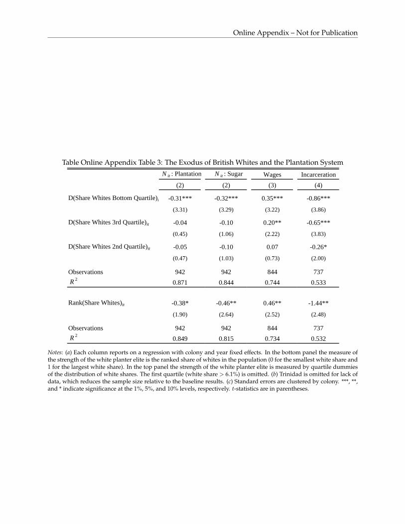
Online Appendix – Not for Publication

Table Online Appendix Table 3: The Exodus of British Whites and the Plantation System

N it : Plantation N it : Sugar Wages Incarceration

(2) (2) (3) (4)

D(Share Whites Bottom Quartile)i -0.31*** -0.32*** 0.35*** -0.86***

(3.31) (3.29) (3.22) (3.86)

D(Share Whites 3rd Quartile)it -0.04 -0.10 0.20** -0.65***

(0.45) (1.06) (2.22) (3.83)

D(Share Whites 2nd Quartile)it -0.05 -0.10 0.07 -0.26*

(0.47) (1.03) (0.73) (2.00)

Observations 942 942 844 737

R 20.871 0.844 0.744 0.533

Rank(Share Whites)it -0.38* -0.46** 0.46** -1.44**

(1.90) (2.64) (2.52) (2.48)

Observations 942 942 844 737

R 20.849 0.815 0.734 0.532

Notes: (a) Each column reports on a regression with colony and year fixed effects. In the bottom panel the measure ofthe strength of the white planter elite is the ranked share of whites in the population (0 for the smallest white share and1 for the largest white share). In the top panel the strength of the white planter elite is measured by quartile dummiesof the distribution of white shares. The first quartile (white share > 6.1%) is omitted. (b) Trinidad is omitted for lack ofdata, which reduces the sample size relative to the baseline results. (c) Standard errors are clustered by colony. ***, **,and * indicate significance at the 1%, 5%, and 10% levels, respectively. t-statistics are in parentheses.

Online Appendix – Not for Publication

Online Appendix C Soil Suitability

We worked with an agronomist to develop a suitability index at the fine spatial resolution de-scribed in section Appendix B.2 (8,144 equally sized cells). For each crop we construct a suitabilityindex following the agronomic literature. For sugar we follow the index suggested in Jayasingheand Yoshida (2010), which includes six factors important for sugar cane (temperature, rainfall,elevation, slope, soil pH, and soil texture). For example, rainfall in the range of 1100–1500 mil-limetres per year is highly suitable for sugar cane, rainfall in the ranges of 950–1100 or 1500–1990is moderately suitable for sugar cane, rainfall in the ranges of 800-950 or 1990–2500 is moderatelyunsuitable for sugar cane, and rainfall in the ranges below 800 or above 2500 is highly unsuitablefor sugar cane. For each factor, categorical suitability bins are constructed for comparability andthe factors are then ranked in their importance, temperature, rainfall, elevation, slope, soil pH, andsoil texture in declining order. The first four categories correlated quite strongly with each other,creating a clean spatial separation of suitability. For example, Online Appendix Figure 5 showsthe topography of Jamaica and compares it with the distribution of suitability. Finally, a weightingis applied to them that reflects this ranking, with the weights summing to 1. We use the weightsfrom Jayasinghe and Yoshida’s (2010) artificial neural network model. These weights make no useof Caribbean land use patterns (weights are based on Sri Lankan data). For each cell, the weightsare used to aggregate the six factors into one of four characterizations of sugar cane suitability:highly suitable, only moderately suitable, unsuitable and totally unsuitable. The vast majority ofthe cells in our colonies are either highly or moderately suitable. Very little Caribbean land wastotally unsuitable for sugar since the climatic conditions were so ideal. (The Jamaican highlandsin Figure 2 form an exception because they get exceptionally cold by Caribbean standards.) Wetherefore focus in the paper on land that is highly suitable or rather the share of land that is highlysuitable.

We understand well which agro-climatic conditions determine suitability for all of our othercrops. Both the agro-climatic conditions and their mapping into suitability are crop-specific. Thisinformation is off-the-shelf available. Online appendix tables Online Appendix Table 4 and OnlineAppendix Table 5 show the suitability-ranges for each input for our four most important crops, aswell as the sources for this coding. The variables given the climactic and soil conditions for eachplot of land are, for cocoa, minimum temperature, maximum temperature, precipitation, numberof months with precipitation less than 100mm, soil depth, soil pH, forest cover (cocoa trees preferto be shaded), and elevation. For lime these variables are temperature, rainfall, soil pH, soil depth,soil texture (degree of sand and clay), slope, and elevation. For arrowroot, temperature, rainfall,soil pH, soil texture, and elevation. For livestock, meaning for the grasses used by livestock,temperature, rainfall, soil pH, elevation, slope, and humidity. For cotton, temperature, rainfall,soil pH, elevation, slope, and humidity. For fruit, temperature, rainfall, soil pH, soil depth, soiltexture, slope, and elevation.

The challenge for the West Indies was obtaining all necessary agro-climatic data at a fineenough spatial resolution. With the help of an agronomist we were able to do so. Data on elevationand slope are from the SRTM 90m Digital Elevation Database at http://www.cgiar-csi.org/data/srtm-90m-digital-elevation-database-v4-1. Data on temperature and rainfallare from the GPCP Version 2.2 Combined Precipitation Data Set at http://www.esrl.noaa.gov/psd/data/gridded/data.gpcp.html. Data on soil texture and pH levels are from theFAO/UNECO World Soil Dataset http://www.fao.org/climatechange/54273/en/. Asa point of comparison, we ended up with 61,421 cells of 604 square-meters for the British WestIndies.

In Online Appendix Table 4, we describe how each island i’s suitability for crop g is estimated

Online Appendix – Not for Publication

from i’s agro-climatic conditions as they affect g, with the sources for these codings listed in OnlineAppendix Table 5. Key is the large variation across islands in some geographic characteristics likeelevation and soil. The importance of elevation for sugar suitability is illustrated by comparisonof top and bottom panel of Online Appendix Figure 5, which shows that sugar suitable land inJamaica was largely on the low-elevation coastal plains. The Caribbean is divided into three islandchains: Most British Caribbean colonies–Dominica, the British Virgin Islands, Grenada, Montser-rat, Nevis, St. Kitts, St. Lucia, and St. Vincent–belonged to the inner chain of the Lesser Antilles,which is volcanic and mountainous. Jamaica was the only British colony in the Greater Antilles(the others are Cuba, Haiti and the Dominican Republic), which are large islands also with moun-tainous interiors. The outer chain of Lesser Antilles–Anguilla, Bahamas, Barbados, Turks andCaicos–consists of flat limestone. Limestone had the great advantage that it was flat, but mostof the outer chain – with the exception of Barbados–was of such low elevation that it was veryvulnerable to salination from storm surges.

For our identification strategy, we proxy plantation land in 1838 with each island’s share ofhighly sugar suitable land. For this, we coded sugar suitability directly based on agriculturalscience literature. Specifically, we follow the artificial neural network method described in Jayas-inghe and Yoshida (2010). We do this because this estimation method makes no use of Caribbeanland use patterns at all (it is based on Sri Lankan data) so that the weights and therefore the indexare entirely exogenous to our data. The method boils down to ranking the six inputs and as-signing them exponential weights: The most important characteristic is assigned weight 0.408 =1+ 1

2+ 1

3+ 1

4+ 1

5+ 1

66 ; the second-most important is assigned weight 0.242 =

12+ 1

3+ 1

4+ 1

5+ 1

66 , and so on.

These weights sum to one so that the aggregate index lies between 1 and 4. Following convention,we then ‘re-bin’ the data by rounding it to the nearest integer so that the index takes on the values 1(highly suitable), 2 (marginally suitable), 3 (marginally unsuitable), and 4 (completely unsuitable).The cross-sectional part of our first instrument Outside Optioni × Caribbean Naval Expendituretis an island’s land share that is not sugar suitable. See Figure 2 for Jamaica. 73

73Guyana is the only colony that is not an island so that in calculating shares of land care must be given to the denom-inator. Guyana had a large hinterland of dense jungle and swampland, most of which was unsuitable for agriculture.We define Guyana’s historical border using the map in Higman (2000, Figure 1.8). We geo-coded this map and calcu-lated Guyana’s sugar suitability share based on these borders. The original map and our geo-coding of it is displayedin Online Appendix Figure 6.

Online Appendix – Not for Publication

Figure Online Appendix Figure 5: Sugar Suitability, and Topography in Jamaica

Notes: The top panel shows elevation for Jamaica. The bottom panel shows the spatial distribution of land that is sugar-suitable (black), only moderately sugar-suitable (dark grey), not sugar-suitable (light grey) and totally sugar-unsuitable(white).

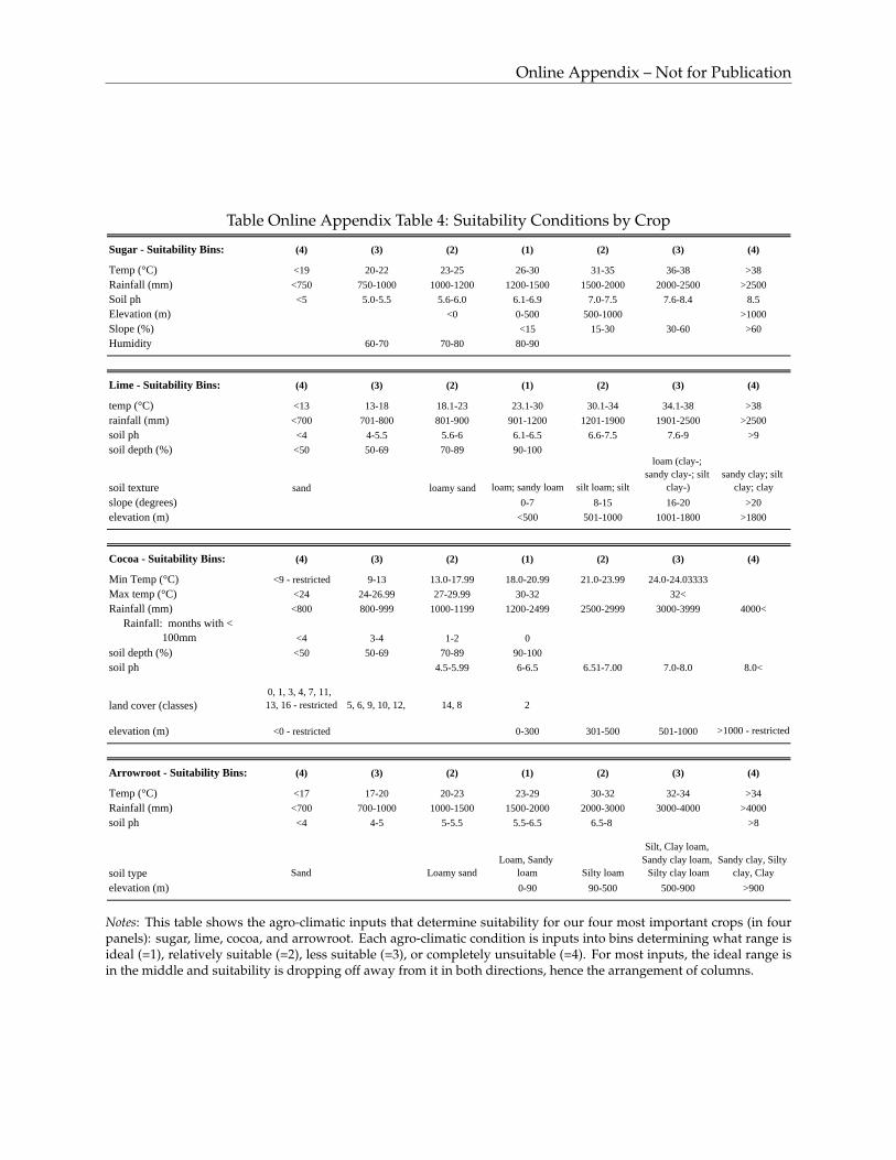
Online Appendix – Not for Publication

Table Online Appendix Table 4: Suitability Conditions by Crop

Sugar - Suitability Bins: (4) (3) (2) (1) (2) (3) (4)

Temp (°C) <19 20-22 23-25 26-30 31-35 36-38 >38

Rainfall (mm) <750 750-1000 1000-1200 1200-1500 1500-2000 2000-2500 >2500

Soil ph <5 5.0-5.5 5.6-6.0 6.1-6.9 7.0-7.5 7.6-8.4 8.5

Elevation (m) <0 0-500 500-1000 >1000

Slope (%) <15 15-30 30-60 >60

Humidity 60-70 70-80 80-90

Lime - Suitability Bins: (4) (3) (2) (1) (2) (3) (4)

temp (°C) <13 13-18 18.1-23 23.1-30 30.1-34 34.1-38 >38

rainfall (mm) <700 701-800 801-900 901-1200 1201-1900 1901-2500 >2500

soil ph <4 4-5.5 5.6-6 6.1-6.5 6.6-7.5 7.6-9 >9

soil depth (%) <50 50-69 70-89 90-100

soil texture sand loamy sand loam; sandy loam silt loam; silt

loam (clay-; sandy clay-; silt

clay-)sandy clay; silt

clay; clay

slope (degrees) 0-7 8-15 16-20 >20

elevation (m) <500 501-1000 1001-1800 >1800

Cocoa - Suitability Bins: (4) (3) (2) (1) (2) (3) (4)

Min Temp (°C) <9 - restricted 9-13 13.0-17.99 18.0-20.99 21.0-23.99 24.0-24.03333

Max temp (°C) <24 24-26.99 27-29.99 30-32 32<

Rainfall (mm) <800 800-999 1000-1199 1200-2499 2500-2999 3000-3999 4000<

Rainfall: months with < 100mm <4 3-4 1-2 0

soil depth (%) <50 50-69 70-89 90-100

soil ph 4.5-5.99 6-6.5 6.51-7.00 7.0-8.0 8.0<

land cover (classes)0, 1, 3, 4, 7, 11, 13, 16 - restricted 5, 6, 9, 10, 12, 14, 8 2

elevation (m) <0 - restricted 0-300 301-500 501-1000 >1000 - restricted

Arrowroot - Suitability Bins: (4) (3) (2) (1) (2) (3) (4)

Temp (°C) <17 17-20 20-23 23-29 30-32 32-34 >34

Rainfall (mm) <700 700-1000 1000-1500 1500-2000 2000-3000 3000-4000 >4000

soil ph <4 4-5 5-5.5 5.5-6.5 6.5-8 >8

soil type Sand Loamy sandLoam, Sandy

loam Silty loam

Silt, Clay loam, Sandy clay loam,

Silty clay loamSandy clay, Silty

clay, Clay

elevation (m) 0-90 90-500 500-900 >900

Notes: This table shows the agro-climatic inputs that determine suitability for our four most important crops (in fourpanels): sugar, lime, cocoa, and arrowroot. Each agro-climatic condition is inputs into bins determining what range isideal (=1), relatively suitable (=2), less suitable (=3), or completely unsuitable (=4). For most inputs, the ideal range isin the middle and suitability is dropping off away from it in both directions, hence the arrangement of columns.

Online Appendix – Not for Publication

Tabl

eO

nlin

eA

ppen

dix

Tabl

e5:

Sour

ces

for

Tabl

eO

nlin

eA

ppen

dix

Tabl

e4

Suga

r:Ja

yasi

nghe

, P.K

.S.C

. and

Mas

ao Y

oshi

da, “

Dev

elop

men

t of T

wo

GIS

-bas

ed M

odel

ing

Fram

ewor

ks to

Iden

tify

Suita

ble

Land

s for

Sug

arca

ne C

ultiv

atio

n,”

Trop

ical

Agr

icul

ture

and

Dev

elop

men

t, 20

10, 5

4 (2

), 51

–61.

Coc

oa:

1. h

ttps:

//ww

w.d

af.q

ld.g

ov.a

u/pl

ants

/frui

t-and

-veg

etab

les/

frui

t-and

-nut

s/ot

her-

frui

t-cro

ps/g

row

ing-

coco

a2.

http

://w

ww

.aca

dem

ia.e

du/9

1297

82/A

_Mul

ti-C

riter

ia_G

IS_S

ite_S

elec

tion_

for_

Sust

aina

ble_

Coc

oa_D

evel

opm

ent_

in_W

est_

Afr

ica_

A_c

ase_

stud

y_of

_Nig

eria

3. h

ttp://

link.

sprin

ger.c

om/a

rticl

e/10

.100

7/s1

0531

-007

-918

3-5

4. h

ttp://

ww

w.ic

co.o

rg/a

bout

-coc

oa/g

row

ing-

coco

a.ht

ml

5. h

ttp://

ww

w.x

ocoa

tl.or

g/tre

e.ht

m

Lim

e:1.

http

://w

ww

.fao.

org/

nr/w

ater

/cro

pinf

o_ci

trus.h

tml

2. h

ttps:

//ww

w.d

af.q

ld.g

ov.a

u/pl

ants

/frui

t-and

-veg

etab

les/

frui

t-and

-nut

s/ci

trus/

citru

s-la

nd-a

ndcl

imat

e-re

quire

men

ts

3. h

ttp://

afgh

anag

.ucd

avis

.edu

/a_h

ortic

ultu

re/fr

uits

-tree

s/ci

trus/

fact

shee

ts/F

S_Fr

uit_

Citr

us_s

ite_s

elec

tion.

doc

4. h

ttp://

ww

w.c

rec.

ifas.u

fl.ed

u/ac

adem

ics/

clas

ses/

hos6

545/

pdf/m

ende

l_19

69.p

df5.

http

://w

ww

.nda

.agr

ic.z

a/do

cs/In

fopa

ks/C

ultiv

atin

gCitr

us.p

df

Arr

owro

ot:

1. h

ttp://

jero

meh

andl

er.o

rg/w

p-co

nten

t/upl

oads

/200

9/07

/Arr

owro

ot-H

isto

ry-7

1.pd

f2.

http

://w

ww

.pro

ta4u

.org

/pro

tav8

.asp

?h=M

4&t=

Mar

anta

,aru

ndin

acea

&p=

Mar

anta

+aru

ndin

acea

3. h

ttp://

rfca

rchi

ves.o

rg.a

u/N

ext/F

ruits

/Veg

etab

les/

Arr

owro

ot9-

96.h

tm4.

http

://tro

pica

l.the

fern

s.inf

o/vi

ewtro

pica

l.php

?id=

Mar

anta

+aru

ndin

acea

Not

es:T

his

tabl

elis

tsth

em

ain

sour

ces

that

dete

rmin

edth

eco

ding

ofsu

itab

ility

bins

inon

line

appe

ndix

tabl

eO

nlin

eA

ppen

dix

Tabl

e4.

Online Appendix – Not for Publication

Figure Online Appendix Figure 6: Guyana

Notes: The left panel shows the historical boundaries of Guyana as dashed lines. The panel is from Higman (2000,figure 1.8). The right panel shows the results of geo-coding the map.

Figure Online Appendix Figure 7: Initial Conditions and Sugar’s End-of-Period (1913) ExportShare

St. Vincent Dominica

St. Lucia Tobago

Jamaica

Trinidad

Montserrat Grenada

Guyana St. Kitts

Antigua

Nevis

Virgin Is.

Barbados

0.0

0.2

0.4

0.6

0.8

1.0

0.0 0.2 0.4 0.6 0.8 1.0

Shar

e of

Sug

ar in

Tot

al E

xpor

ts, 1

913

Potential Outside Option (share of sugar-unsuitable land)

Notes: Each point is a colony’s Nit in 1913 plotted against its share of land that is unsuitable for sugar cane cultivation,which is a proxy for the share of all land that was unused in 1838. The −45◦ line provides a benchmark. Plantationshares for Nevis (Tobago) are extrapolated out to 1913 using 1882 (1898) data and growth rates from St. Kitts (Trinidad).

Online Appendix – Not for Publication

Online Appendix D Export Price Data

We need crop prices for the gravity estimation in in Appendix B.2. For a given crop, prices (exportunit values) are based on the export data of the largest exporter of the crop. This ensures thatthe prices are based on large volumes. Livestock: There are many types of livestock. We use themost important of these, namely cattle and horses. Using Virgin Islands exports we build priceseries separately for cattle and horses. Arrowroot prices are based primarily on export data fromJamaica (1838-1854) and St. Vincent (1855-1913). The St. Vincent Blue Book data are augmented bySt. Vincent data reported in the Journal of the Royal Society of Arts (1873). Cocoa prices are basedon export data from Granada and Trinidad. Cotton prices are based on export data from Guyana(1838–1844) and Granada (1856–1913).74 Bananas, oranges, pimento, coffee, lumber, and ginger pricesare based on export data from Jamaica. For other spices (predominantly cloves, mace and nutmeg),prices are based on export data from Granada. Charcoal prices are based on export data fromthe Virgin Islands. Asphalt and balata (a natural tar) are based on export data from Trinidad andGuyana, respectively. Lime juice prices are based on export data from Jamaica (1838–61), Monserrat(1862–78), Dominica (1872–87), Monserrat (1872–78), and Jamaica (1891–1912). Because lime wasexported in many different forms, we made extensive use of contemporary surveys of prices inorder to develop a meaningful price series. Coconut prices are based on export data from Jamaica(1844–58), Tobago (1862–63), Tobago and Trinidad (1868–81), and Tobago, Trinidad and Jamaica(1882–1912).

Finally, Online Appendix Table 6 reports the coefficients from estimating the gravity equa-tion (16) in Appendix B.2.

74This is the only crop that appears in Jacks (2005). Our price series is is highly correlated with the Jacks (2005) seriesexcept during the Civil War years.

Online Appendix – Not for Publication

Table Online Appendix Table 6: Estimates of the Gravity Equation (16) — Recovering ri(pt, τ s)

θ ln(p gt /p st ) 2.30*** (3.93)

θ ln(τpg /τ

sg ) Pl git

g = cocoa 20.36*** g = arrowroot 16.43***(3.24) (4.40)

g = coffee 3.40*** g = lime 3.79(5.45) (1.50)

g = fruit 9.14 g = livestock -5.83(1.71) (1.45)

Observations 7,126 R-squared 0.863

Notes: This table reports the parameters of interest from equation (16). The dependent vari-able is ln(xgit) − ln(xsit) where the s subscript stands for sugar. The first row is the co-efficient θ on ln pgt/pst. The remaining rows are the coefficients θ ln(τpg /τ

sg ) on Plgit. The

number of observations is non-sugar crops (7) times colony-year pairs (1018).

Online Appendix – Not for Publication

Figure Online Appendix Figure 8: Hurricanes and the Decline of Virgin Islands Sugar

0.2

.4.6

.81

(sug

ar e

xpor

ts) /

(tot

al e

xpor

ts)

.. . .

1838 1848 1852 1867 1871 1889Notes: Vertical lines are hurricane dates. Sugar did not re-cover after 1889.

Online Appendix E Hurricanes

Online Appendix E.1 The Impact of Hurricanes

Figure Online Appendix Figure 8 vividly displays the long-lasting effects of hurricane landfallsfor the Virgin Islands, showing the evolution of sugar as a share of exports over time. Verticallines are major hurricane dates. Destructive hurricanes in 1848 and especially 1852 decimated theindustry. Because of the long-lasting effects of these early hurricanes, later ones could not fur-ther weaken an already collapsed plantation system. To operationalize the impact of hurricaneswe need to capture the permanence of their impact and also the fact that a hurricane that hit analready decimated plantation economy could not do much further damage. We therefore con-structed an instrument HDIit that assigned each Caribbean hurricane landfall a damage index.HDIit measures a hurricane’s effect on the sugar-economy as the two-year log change in sugarexports around the landfall year t and then stays constant thereafter.75 One concern with usinghurricanes as an instrument is that they plausibly could have had direct effects on wages. How-ever, such direct effects would have been only contemporaneous to the years of or immediatelyafter a hurricane, whereas we code the effect ofHDIit as persistent by construction in order to cap-ture hurricanes’ persistent effects discussed above. It turns out that we need to include hurricanesin our estimation in order to fit the variation in Nit only for the Virgin Islands.

Online Appendix E.2 Details of Hurricane Damage Construction

We coded up all hurricanes landfall on the islands during our period of study from the annualhurricane track maps published by the United States National Hurricane Center (2014) and, for

75The logic for using two-year changes is as follows. We know from our data that crops almost always bounced backwithin a year after a major storm. In the first year there are declines in sugar exports both because of crop damageand because of infrastructure damage. In the second year, the crop comes back only to the extent allowed by theinfrastructure damage so it is two years of depressed exports that speaks to the infrastructure damage. Let xsit becolony i’s sugar exports in year t and let t0 be the date of a hurricane so that ∆i(t0) ≡ lnxsi,t0−1 − lnxsi,t0+1 is thetwo-year log change in sugar exports. If sugar exports increased after the hurricane (∆i(t0) < 0) then we set ∆i(t0) tozero. Our hurricane damage index instrument is HDIit ≡ ∆i(t0) for t ≥ t0 and HDIit ≡ 0 for t < t0.

Online Appendix – Not for Publication

the pre-1851 period, by Tannehill (1938). Hurricane tracks were digitized and GIS software usedto identify landfalls.

The hurricane damage index is max[ 0 , (lnxsi,t0−1 − lnxsi,t0+1) ] where t0 is the year of thehurricane and xsi,t0−1 and xsi,t0+1 are sugar exports by colony i in the years before and after thehurricane. While the year of the hurricane is known, the resulting fall in exports is sometimesreported in the next Blue Book year because Blue Books do not necessarily report data on a calendarbasis. Where the fall in exports happened in the year after the hurricane, we increment t0 by oneyear. This occurs for Jamaica (1874, 1880, 1896), Montserrat (1851), St. Lucia (1875, 1894), andSt. Kitts (1910). For example, the Jamaican hurricane of 1896 is associated with sugar exports of£290,000 (1896), £219,000 (1897) and £261,000 (1898) so we set t0 = 1897.

What follows is a list of the 28 hurricanes along with the year (t0), the two-year log changein sugar exports (∆i(t0)), and an indicator for whether it was a major hurricane (*). We groupcolonies into three groups:

1. Complete collapse of sugar: Virgin Islands 1848 (1.18*), 1852 (1.51*), 1867∗ (6.18*), 1871∗

(0.00), 1889 (0.00); Montserrat 1851 (0.64), 1889 (0.25), 1899∗ (0.00), 1909 (0.00); Grenada 1856(0.00); Dominica 1883∗ (0.23*), 1903 (0.68); St. Vincent 1886 (0.48), 1898 (0.75).

2. Moderate decline of sugar: Tobago none; St. Lucia 1875 (0.00), 1894 (0.09); Trinidad 1878(0.08); Jamaica 1874 (0.00 ), 1880 (0.00), 1886 (0.00), 1896 (0.10), 1903∗ (0.38*), 1910 (0.05).

3. No decline of sugar: Antigua 1910 (0.18); Barbados none; Guyana none; St. Kitts 1859(0.0049), 1889 (0.08), 1908 (0.00), 1910 (0.15).

Looking across the 28 hurricanes that made landfall in the British West Indies during 1838–1913,what stands out is the Virgin Islands: It was hit repeatedly, it was hit early on, and the hits didmajor damage.

There are four hurricanes with historical ambiguities. (1) Virgin Islands 1848: Dookhan (1975)claims that there was a hurricane in the Virgin Islands in 1842 and makes no mention of the 1848hurricane. Using his hurricane dating rather Tannehill’s (1938) makes no difference to our results.(2) Barbados and Montserrat 1899: This hurricane was extremely powerful, causing many deathsin Montserrat and Barbados. The National Hurricane Centre track for this hurricane shows thatit made landfall in Montserrat, but not Barbados. The hurricane had little impact on Blue Bookexports in either location. To investigate potential measurement error we experimented with cod-ing this hurricane as having a large damage index (1.00) in both colonies. This improves our re-sults. (3) Antigua 1871: This hurricane overlapped with the disastrous drought of 1870–1874. SeeBerland, Metcalfe and Endfield (2013, Figure 4). Contemporaries commented much more on thedrought than on the hurricane (Berland et al., 2013, 1338). Indeed, there is no mention of the hurri-cane in the 1871 Antigua Blue Book listing of Parliamentary Acts, but there is a listing of an Act en-titled “An Act to raise the sum of £2500 for the Antigua Water Works.” Finally, when the droughtended, agricultural output completely rebounded: Sugar exports were £228,000 (1870), £239,000(1871), £136,000 (1872), £153,000 (1873), £96,000 (1874, the worst year of the drought), and £243,000(1875). In short, the cause of the decline in sugar exports was the drought, not the hurricane. Wetherefore code it as a 0. (4) Grenada 1856: This hurricane is assigned a small damage index be-cause its impacts are confounded with the massive cholera epidemic that began in mid-June 1854(too late to affect the 1854 sugar crop) and carried on through 1855. Sugar exports were £130,000(1854), £82,000 (1855), £90,000 (1856), and £148,000 (1857). Hence lnxis,1856−1 − lnxi,s,1856+1 < 0.If we assign this hurricane a large damage index (1.00) our results improve slightly.

Online Appendix – Not for Publication

Online Appendix F The Impact of Productivity Growth on N ∗ and w

As discussed in detail in Online Appendix H.3, productivity grew much more rapidly in sugarthan in smallhold crops. We therefore assume that Caribbean productivity increased in a way thatraised plantation revenues from r(p, τp) to ϕr(p, τp) and raised smallhold revenues from r(p, τ s)to ϕδr(p, τ s) for some ϕ > 1 and δ ∈ (0, 1). Equation (2) now becomes

w = ϕδr(p, τ s)− C (17)

and equation (3) now becomes

π(C,N ;ϕ) = l(N)[ϕr(p, τp)− ϕδr(p, τ s) + C

]− Cγ/N . (18)

It follows that

πϕ = l(N)[r(p, τp)− δϕδ−1r(p, τ s)

]> l(N) [r(p, τp)− r(p, τ s)] > 0

where the first inequality follows from δϕδ−1 < 1 and the second inequality follows from the factthat in an equilibrium withN∗ > 0, revenues per standard plot size are higher on plantations thansmallholds. Plugging this into the protection-for-sale welfare function (equation 4) and differenti-ating shows that the optimal level of coercion C∗(N) does not depend on ϕ. From equation (17),∂w/∂ϕ > 0. From equation (18), πN (N∗)(∂N∗/∂ϕ) + πϕ = 0 or ∂N∗/∂ϕ = −πϕ/πN (N∗) > 0where we have used πN (N∗) < 0. Thus, both N∗ and w rise.

Online Appendix – Not for Publication

Online Appendix G Measuring Wages, Wage Frequency, and In-KindPayments

In Montserrat, wages appear to have been commonly accompanied by access to a cottage or use ofprovision lands, for which we do not know the monetary value (Fergus, 1994). All of our readingssuggested that this norm in Montserrat was in place throughout our period so that it is absorbed inthe Montserrat colony fixed effect. Wages sometimes included an in-kind component that usuallyinvolved a cottage and a small plot. For two-thirds of our sample the Blue Books indicate whetherthe wage includes in-kind payments. Only 9% of these observations include in-kind payments.Panel A of Online Appendix Table 7 shows that our results are robust to an adjustment for in-kindpayments.

In a handful of cases, wages were reported as weekly or monthly, in which case we dividedthem by 5 or 20, as this was the explicit conversion stated in the Blue Books. Panels B and C ofOnline Appendix Table 7 show that none of our results depend on this specific conversion factor.Online Appendix Table 7 shows that none of our results depend on this specific conversion factor.In a few other cases, wages were reported as a range, in which case we used the midpoint. Wagesare sticky so we also considered moving averages of 1 to 3 years. This strengthens our results.

Online Appendix – Not for Publication

Table Online Appendix Table 7: Robustness Checks on Wage Variable

Panel A. Multiplying wit × 1.2 when ”home and ground” providedh&glog wage - home & ground OLS IV

(1) (2) (3) (4) (5) (6) (7) (8)

Nit: Sugar Exports as -0.3714 -0.3839 -0.5971 -0.5891 Share of Total Exports [0.0078] [0.0112] [0.0043] [0.0066]

Nit: Plantation Exports as -0.5229 -0.5483 -0.9306 -0.9700 Share of Total Exports [0.0027] [0.0034] [0.0011] [0.0015]

Time Controls t + t2 t-fe t + t2 t-fe t + t2 t-fe t + t2 t-feObservations 908 908 908 908 908 908 908 908F Statistic (Instruments) 23.2832 21.6359 24.7038 22.0467R-squared 0.724 0.771 0.731 0.779

lowerlog wage - lower bound OLS IV

(1) (2) (3) (4) (5) (6) (7) (8)

Nit: Sugar Exports as -0.2957 -0.3093 -0.5208 -0.5292 Share of Total Exports [0.0527] [0.0711] [0.0133] [0.0211]

Nit: Plantation Exports as -0.4434 -0.4635 -0.8564 -0.9261 Share of Total Exports [0.0210] [0.0288] [0.0026] [0.0037]

Time Controls t + t2 t-fe t + t2 t-fe t + t2 t-fe t + t2 t-feObservations 908 908 908 908 908 908 908 908F Statistic (Instruments) 23.2832 21.6359 24.7038 22.0467R-squared 0.682 0.765 0.689 0.772

upperlog wage - upper bound OLS IV

(1) (2) (3) (4) (5) (6) (7) (8)

Nit: Sugar Exports as -0.4018 -0.4191 -0.6121 -0.5812 Share of Total Exports [0.0040] [0.0047] [0.0038] [0.0075]

Nit: Plantation Exports as -0.5576 -0.5845 -0.9419 -0.9459 Share of Total Exports [0.0016] [0.0013] [0.0010] [0.0019]

Time Controls t + t2 t-fe t + t2 t-fe t + t2 t-fe t + t2 t-feObservations 908 908 908 908 908 908 908 908F Statistic (Instruments) 23.2832 21.6359 24.7038 22.0467R-squared 0.728 0.777 0.735 0.785

Panel B. Discounting Monthly and Weekly Wages More

h&glog wage - home & ground OLS IV

(1) (2) (3) (4) (5) (6) (7) (8)

Nit: Sugar Exports as -0.3714 -0.3839 -0.5971 -0.5891 Share of Total Exports [0.0078] [0.0112] [0.0043] [0.0066]

Nit: Plantation Exports as -0.5229 -0.5483 -0.9306 -0.9700 Share of Total Exports [0.0027] [0.0034] [0.0011] [0.0015]

Time Controls t + t2 t-fe t + t2 t-fe t + t2 t-fe t + t2 t-feObservations 908 908 908 908 908 908 908 908F Statistic (Instruments) 23.2832 21.6359 24.7038 22.0467R-squared 0.724 0.771 0.731 0.779

lowerlog wage - lower bound OLS IV

(1) (2) (3) (4) (5) (6) (7) (8)

Nit: Sugar Exports as -0.2957 -0.3093 -0.5208 -0.5292 Share of Total Exports [0.0527] [0.0711] [0.0133] [0.0211]

Nit: Plantation Exports as -0.4434 -0.4635 -0.8564 -0.9261 Share of Total Exports [0.0210] [0.0288] [0.0026] [0.0037]

Time Controls t + t2 t-fe t + t2 t-fe t + t2 t-fe t + t2 t-feObservations 908 908 908 908 908 908 908 908F Statistic (Instruments) 23.2832 21.6359 24.7038 22.0467R-squared 0.682 0.765 0.689 0.772

upperlog wage - upper bound OLS IV

(1) (2) (3) (4) (5) (6) (7) (8)

Nit: Sugar Exports as -0.4018 -0.4191 -0.6121 -0.5812 Share of Total Exports [0.0040] [0.0047] [0.0038] [0.0075]

Nit: Plantation Exports as -0.5576 -0.5845 -0.9419 -0.9459 Share of Total Exports [0.0016] [0.0013] [0.0010] [0.0019]

Time Controls t + t2 t-fe t + t2 t-fe t + t2 t-fe t + t2 t-feObservations 908 908 908 908 908 908 908 908F Statistic (Instruments) 23.2832 21.6359 24.7038 22.0467R-squared 0.728 0.777 0.735 0.785

Panel C. Discounting Monthly and Weekly Wages Less

h&glog wage - home & ground OLS IV

(1) (2) (3) (4) (5) (6) (7) (8)

Nit: Sugar Exports as -0.3714 -0.3839 -0.5971 -0.5891 Share of Total Exports [0.0078] [0.0112] [0.0043] [0.0066]

Nit: Plantation Exports as -0.5229 -0.5483 -0.9306 -0.9700 Share of Total Exports [0.0027] [0.0034] [0.0011] [0.0015]

Time Controls t + t2 t-fe t + t2 t-fe t + t2 t-fe t + t2 t-feObservations 908 908 908 908 908 908 908 908F Statistic (Instruments) 23.2832 21.6359 24.7038 22.0467R-squared 0.724 0.771 0.731 0.779

lowerlog wage - lower bound OLS IV

(1) (2) (3) (4) (5) (6) (7) (8)

Nit: Sugar Exports as -0.2957 -0.3093 -0.5208 -0.5292 Share of Total Exports [0.0527] [0.0711] [0.0133] [0.0211]

Nit: Plantation Exports as -0.4434 -0.4635 -0.8564 -0.9261 Share of Total Exports [0.0210] [0.0288] [0.0026] [0.0037]

Time Controls t + t2 t-fe t + t2 t-fe t + t2 t-fe t + t2 t-feObservations 908 908 908 908 908 908 908 908F Statistic (Instruments) 23.2832 21.6359 24.7038 22.0467R-squared 0.682 0.765 0.689 0.772

upperlog wage - upper bound OLS IV

(1) (2) (3) (4) (5) (6) (7) (8)

Nit: Sugar Exports as -0.4018 -0.4191 -0.6121 -0.5812 Share of Total Exports [0.0040] [0.0047] [0.0038] [0.0075]

Nit: Plantation Exports as -0.5576 -0.5845 -0.9419 -0.9459 Share of Total Exports [0.0016] [0.0013] [0.0010] [0.0019]

Time Controls t + t2 t-fe t + t2 t-fe t + t2 t-fe t + t2 t-feObservations 908 908 908 908 908 908 908 908F Statistic (Instruments) 23.2832 21.6359 24.7038 22.0467R-squared 0.728 0.777 0.735 0.785

Notes: In Panel A, to check the robustness to the provision of home and ground of this assumption, we multiply wagesby a factor of 1.2 in all colony-years in which the Blue Books explicitly mentioned that ”home and ground” were includedin the wage payments. The factor 1.2 comes from Sewell (1861, 32). Weekly wages in the Blue Books are consistentlyreported as being paid for weeks of five days, and monthly wages as being paid for months of twenty days. In PanelsB and C we check for robustness to variations on those rules. It is possible that five-day work weeks and 20-daywork months paid lip-service to Abolitionists but that effective works weeks and months were longer. In Panel B,we therefore divide weekly Wages by 1/6 and monthly wages by 1/24 instead of the 1/5 and 1/20 conversion ratessuggested in the Blue Books. On the other hand, it may be that weekly and monthly contracts came with unreportedin-kind payments such as right to a garden plot that would not have applied to day workers. In that case, real weeklyand monthly wages would have been higher than daily wages. In Panel C, we therefore experiment with dividingweekly wages by 1/4 and monthly wages by 1/16 instead of the 1/5 and 1/20 conversion rates suggested in the BlueBooks.

Online Appendix – Not for Publication

Online Appendix H Additional Results and Robustness

Online Appendix H.1 The Historical Record on Differential Trends

We begin with a simple question: “Have we missed any cross-colony differences emphasized byhistorians that might predict observed or unobserved differential trends?” The answer is yes. Pop-ulation density is the colony characteristic that is universally identified as central for understand-ing the post-Emancipation evolution of the British West Indies economies (Engerman, 1984, 133).To understand why, recall that the slave trade was abolished in 1807, more than a generation beforethe abolition of slavery in 1838. The lack of a slave trade limited the chief mechanism for equaliz-ing slave prices and marginal productivities across colonies. For example, Trinidad and Guyanaturned to slave-based sugar cultivation only after becoming British in 1797 and 1803, respectively.Their post-1807 slave populations were therefore smaller than desired by planters. Correspond-ingly, their population densities were the lowest among our 14 colonies and their slave prices werethe highest. As a result, pre-Emancipation population density and slave prices were widely under-stood to predict how wages and hence plantation success would evolve post-Emancipation, e.g.,Merivale’s famous 1841 lectures (Merivale, 1861, 312–317). Modern historians have also focussedon population densities and slave prices, e.g., Engerman (1984) and Eltis, Lewis and Richardson(2005).

The literature identifies population density and slave prices, then, as the key colony charac-teristics for understanding the post-Emancipation evolution of our colonies. Importantly for ourpurposes, these initial colony characteristics are the most obvious source of unobserved differen-tial trends in labour supply. Colonies with initially abundant labour may have had unobserveddifferential declines in labour supply while colonies with initially scarce labour may have had un-observed differential increases in labour supply.76 This observation means that the main factorsemphasized by contemporaries and historians are labour supply shocks and so are factors that arelikely to explain away are results. Since, as we will show, our results are not sensitive to control-ling for these factors, it is unlikely that our results are sensitive to other unobserved differentialtrends in labour supply.

Online Appendix H.2 Differential Trends in Labour Supply

We measure population density as the pre-Emancipation population divided by the area of thecolony. We denote this by (Pop Density)1836. Data are from Martin (1839) and are based onpre-1838 Blue Books. Slave prices are for head slaves and are denoted by (Slave Price)1836. Dataare also from Martin (1839) and are based on the reliable 1836 assessment of slave prices. Weconsider the possibility that our instrument Oi ·W t is correlated with (Slave Price)1836 ·W t and(Pop Density)1836 ·W t so that, as in point 3 above, Oi ·W t is correlated with a predictor of differ-ential trends in labour supply and TSLS is negatively biased.

To eliminate this bias we include (Slave Price)1836 ·W t or (Pop Density)1836 ·W t in both the firstand second stages. The new TSLS results appear in Panels A and B of Online Appendix Table 8.The first observation is that these variables are statistically insignificant. The second observation isthat the estimated TSLS coefficients on Nit are very similar to our baseline results in Table 4. Thissuggests that there is no conditional correlation between Nit and these predictors of differentialtrends in labour supply. It follows that our results are not explained away by the most important historicalcandidate for unobserved differential trends in labour supply.

76For example, over time labour may have illegally migrated from slave-abundant to slave-scarce locations.

Online Appendix – Not for Publication

Noting that W t trends, it is possible that population density and slave price would have per-formed better with a more flexible specification of the differential trends. To investigate, we addflexibility by interacting (Pop Density)1836 and (Slave Price)1836 with a linear time trend t and in-cluding (Pop Density)1836 · t or (Slave Price)1836 · t in the first and second stages. The new TSLSresults appear in Panels C and D of Online Appendix Table 8. The first observation is that thesevariables are also statistically insignificant. The second and more important observation is that theinclusion of these variables has no impact on our TSLS estimates of the coefficients on Nit. Again,there appears to be no correlation between Nit and these predictors of differential trends in laboursupply, making it unlikely that our results are explained away by unobserved differential trendsin labour supply.

Online Appendix – Not for Publication

Online Appendix H.3 Other Possible Differential Trends

The growth of industry, commerce, and urbanization all potentially drew labour away from theplantation economy. Differential growth in these acts as a differential plantation labour supplytrend that could explain away our results. However, the historical record on these trends is veryclear: Industry, commerce, and urbanization remained at very low levels throughout our period in everycolony. We document this in Appendix B.1. To further examine this, Table A1 reports a regres-sion of the share of the population employed in commerce on Nit and colony fixed effects. Thecoefficient on Nit is statistically insignificant. Likewise when the dependent variable is the shareof the population employed in manufacturing. Panel B repeats the exercise with Nit replaced byour instrument Oi ·W t and the conclusions are the same: Employment in commerce and manu-facturing are not correlated with our instrument. (See point 3 at the start of this section.) Thus,there is no evidence in the historical literature or data that differential trends in commerce andmanufacturing could bias our IV results.

As for urbanization, it did not begin until the very end of our sample, if not later. Whileurbanization statistics are scarce, in the most populous colony of Jamaica, Eisner (1961, 181–186)carefully documents that there was no trend in urbanization before 1913.

The final potential differential trend we examine is productivity. There is a large literature onproductivity growth in sugar. During our period all aspects of sugar processing became mech-anized, from cane crushing to the evaporation of juice into sugar crystals. This mechanizationexplains why labour productivity in sugar grew throughout our period, while there was no com-parable mechanization in any other Caribbean crop.77

What impact does unobserved productivity improvements in sugar have on our estimates? Ifthere were unobserved differential trends in sugar productivity, these would work against us findinga negative impact of planter power on wages. Sugar productivity growth leads to more sugar outputper unit of labour. This in turn shifts out labour demand, which increases both wages wit and theequilibrium quantity of labour. Higher productivity and more labour inputs both push for higherNit. That is, both Nit and wit must rise. This is proved in Online Appendix F. The productivity-induced positive correlation betweenNit and wit makes the TSLS estimate of the coefficient onNit

more positive than the ‘true’ coefficient. That is, it works against our finding.In summary, going through the list of candidate differential trends across colonies, we can in

all cases show that they either did not exist, or do not affect our results, or would bias us awayfrom finding a negative effect of Nit on wit.

77Important plantation crops all experienced productivity gains associated with improved varieties, identificationof ideal agro-climactic conditions, disease control, transportation, and post-harvest processing. However, the onlyexplosive productivity growth was in post-harvest sugar processing. Compare the long list of inventions related tosugar in Deerr (1950, 534–590) to the inventions for cocoa and arrowroot in Knapp (1920) and Handler (1965). Note thatsugar innovations all originated in Europe and the United States, largely in response to the 19th century developmentof beet sugar. Thus, the innovations were exogenous to the Caribbean.

Online Appendix – Not for Publication

Table Online Appendix Table 8: Examining the Exclusion RestrictionOutcome w it : log wage C it : Incarceration (per Cap.)

t + t2 t-fe t + t2 t-fe t + t2 t-fe t + t2 t-fe

(1) (2) (3) (4) (5) (6) (7) (8)

Panel AN it (Share of Exports) -0.5518 -0.5617 -0.8449 -0.8777 1.2288 0.8559 1.5875 1.1269

[0.0001] [0.0109] [0.0000] [0.0006] [0.0004] [0.0299] [0.0000] [0.0059]

{0.010} {0.039} {0.005} {0.035} {0.001} {0.012} {0.008} {0.02}

(Pop Density)1836,i x 0.0158 0.0042 0.0357 0.0278 0.0542 -0.0098 -0.0152 -0.0708

English Exports [0.5239] [0.9056] [0.0524] [0.2793] [0.1329] [0.8705] [0.4898] [0.1555]

F Statistic (Instruments) 22.9 30.3 28.2 34.1 19.0 31.6 19.2 29.7

Panel BN it (Share of Exports) -0.5605 -0.5564 -0.9413 -0.994 1.0563 0.8941 1.6755 1.4941

[0.0014] [0.0026] [0.0001] [0.0002] [0.0001] [0.0075] [0.0000] [0.0009]

{0.064} {0.139} {0.047} {0.046} {0.004} {0.023} {0.009} {0.024}

Slave Price1836,i x -0.0004 -0.0008 0.0008 0.0008 0.0011 0.0021 -0.0024 -0.0016

English Exports [0.7992] [0.6609] [0.5067] [0.6173] [0.6686] [0.4259] [0.4686] [0.6214]

F Statistic (Instruments) 24.5 22.1 17.7 13.7 21.9 21.8 16.8 15.7

Panel CN it (Share of Exports) -0.5516 -0.5666 -0.8253 -0.8866 1.0544 0.7802 1.2852 1.0607

[0.0060] [0.0135] [0.0001] [0.0009] [0.0200] [0.0643] [0.0035] [0.0159]

{0.0197} {0.0165} {0.0115} {0.0167} {0.0358} {0.1488} {0.0219} {0.1306}

(Pop Density)1836,i x t 0.0003 0.0001 0.0009 0.0007 -0.0001 -0.0009 -0.0024 -0.0025

[0.8015] [0.9502] [0.2053] [0.3617] [0.9621] [0.6880] [0.1539] [0.1502]

F Statistic (Instruments) 26.7 28.9 36.2 35.5 21.3 28.3 24.0 30.5

Panel DN it (Share of Exports) -0.5622 -0.5543 -0.9689 -0.9959 1.0568 0.8946 1.6753 1.4907

[0.0095] [0.0164] [0.0029] [0.0051] [0.0034] [0.0071] [0.0019] [0.0010]

{0.096} {0.0824} {0.064} {0.0612} {0.016} {0.0382} {0.0143} {0.0339}

Slave Price1836,i x t -0.0000 -0.0000 0.0000 0.0000 0.0001 0.0001 -0.0000 -0.0000

[0.9226] [0.7069] [0.4448] [0.6846] [0.2004] [0.3410] [0.7991] [0.7652]

F Statistic (Instruments) 21.8 21.0 14.4 13.2 20.0 20.8 15.0 15.1

N it : Sugar N it : Plantation N it : Sugar N it : Plantation

Notes: Each panel in this table replicates Table 4, but with the indicated additional regressor included both here in thesecond stage and in the first stage (not reported). The additional covariates in Table 4 are also included but not reported.

Online Appendix – Not for Publication

Online Appendix H.4 Time Interactions with Other Geographic Characteristics

In Table Online Appendix Table 9, we investigate the robustness of our main results in Table 4 toallowing for a variety of geographic features having time-varying effects on our outcomes. To thisend, we add in each panel an interaction between one geographic feature at a time (slope in PanelsA and D, elevation in B and E, mean temperature C and F) with either the time-varying part ofour instrument W t (in Panels A–C), or with a time trend (Panels D–F).

Online Appendix – Not for Publication

Table Online Appendix Table 9: Time Interactions with Other Geographic Characteristics

Outcome w it : log wage C it : Incarceration (per Cap.)

N it

Time Controls t + t2 t-fe t + t2 t-fe t + t2 t-fe t + t2 t-fe

(1) (2) (3) (4) (5) (6) (7) (8)

Panel AN it (Share of Exports) -0.5184 -0.5933 -0.7553 -0.9404 0.8253 0.7056 0.8936 0.7863

[0.0760] [0.1078] [0.0001] [0.0003] [0.0209] [0.0662] [0.0398] [0.0849]

Slope i x 0.0043 0.0031 0.0032 0.0001 0.0038 0.0069 0.0002 0.0037

English Exports [0.6942] [0.8349] [0.6265] [0.9931] [0.7671] [0.6484] [0.9900] [0.7858]

F Statistic (Instruments) 65.6 53.3 18.5 14.2 33.8 35.5 10.5 9.0

Panel BN it (Share of Exports) -0.5000 -0.5837 -0.7533 -0.9388 0.8241 0.6397 0.9347 0.7880

[0.0928] [0.1160] [0.0001] [0.0004] [0.0165] [0.0938] [0.0161] [0.0837]

Elevation i x 0.0002 0.0001 0.0002 0.0000 0.0001 0.0000 0.0000 -0.0000

English Exports [0.5927] [0.7975] [0.4895] [0.9286] [0.7472] [0.9836] [0.9409] [0.9589]

F Statistic (Instruments) 55.8 51.6 14.8 13.5 29.1 34.5 8.3 8.3

Panel CN it (Share of Exports) -0.6820 -0.7835 -0.7781 -0.9588 0.7976 0.6941 0.9156 0.7977

[0.0043] [0.0183] [0.0000] [0.0000] [0.0618] [0.0979] [0.0382] [0.0804]

Mean Temperature i x -0.0004 -0.0005 -0.0001 -0.0002 0.0001 0.0002 -0.0003 -0.0001

English Exports [0.3305] [0.3593] [0.6476] [0.5241] [0.9346] [0.7794] [0.6076] [0.8325]

F Statistic (Instruments) 39.8 25.1 7.3 5.8 30.1 24.3 5.9 5.1

Panel DN it (Share of Exports) -0.6647 -0.7781 -0.7825 -0.9588 0.7850 0.6183 0.9208 0.7818

[0.0053] [0.0177] [0.0000] [0.0000] [0.0646] [0.1797] [0.0376] [0.1163]

Slope i x t -0.0000 -0.0000 -0.0000 -0.0000 0.0000 -0.0000 -0.0000 -0.0000

[0.4121] [0.3739] [0.7543] [0.5175] [0.9770] [0.9258] [0.5713] [0.6150]

F Statistic (Instruments) 28.2 23.4 6.5 5.8 23.0 23.0 5.4 5.0

Panel EN it (Share of Exports) -0.5440 -0.7643 -0.8388 -1.0035 0.7773 0.6208 1.1298 0.8183

[0.0009] [0.0067] [0.0000] [0.0001] [0.0025] [0.0656] [0.0000] [0.0359]

Elevationi x t -0.0023 0.0608 -0.0055 0.0116 -0.0186 0.0053 -0.0137 0.0509

[0.6518] [0.2573] [0.2380] [0.7735] [0.0030] [0.9484] [0.0353] [0.4583]

F Statistic (Instruments) 48.3 48.8 8.6 8.9 41.3 100.6 7.7 13.3

Panel FN it (Share of Exports) -0.6839 -0.7555 -0.8627 -1.0024 0.7340 0.5540 0.9521 0.7561

[0.0005] [0.0067] [0.0000] [0.0001] [0.0304] [0.1278] [0.0094] [0.0785]

Mean Temperaturei x t 0.0015 0.0017 0.0002 0.0003 0.0006 0.0009 0.0021 0.0020

[0.2476] [0.2799] [0.8044] [0.7706] [0.7921] [0.7276] [0.2567] [0.3406]

F Statistic (Instruments) 52.6 47.1 9.0 8.4 94.6 102.3 12.8 12.9

N it : Sugar N it : Plantation N it : Sugar N it : Plantation

Notes: Each panel in this table replicates Table 4, adding as a robustness check an interaction between one geographicfeature at a time (slope in Panels A and D, elevation in B and E, mean temperature C and F) with either the time-varyingpart of our instrument W t (in Panels A–C), or with a time trend (Panels D–F).

Online Appendix – Not for Publication

Online Appendix H.5 Parish-Level Results

Online Appendix H.5.1 Parish-Level Equivalent of Main Results

Pushing skepticism further, it is possible that our results are spuriously driven by differentialtrends across colonies which can only be captured by a full set of colony-year fixed effects. Thiswould mean that nothing can be identified with our colony-year data. Of course we do not believethis: The point of our British West Indies sample of sugar colonies is exactly that the colonies werevirtually identical in all but a quantifiable set of agro-climactic factors and subject to commonshocks. Nevertheless, we suspend our disbelief and now move to parish-level, sub-colony dataso that we can include a full set of colony-year fixed effects.78 All of our colonies have parish-leveladministrative units. We observe data for just over 100 parishes in 11 colonies for a total of 2,240observations.79

There are no data for Guyana, Trinidad or the Virgin Islands. The number of parishes by colonyand year appear in Online Appendix Table 10. Because our agricultural suitability data are at thesub-parish level, we can compute Oi at the parish level simply by geocoding parish boundaries.For parish p in colony i, let Opi be the parish counterpart to Oi. While we do not have wage orcoercion data at the parish level, we do have mortality rates. We will find that the weakening of theplantation system led to a fall in mortality rates and interpret this to mean that the weakening ledto some combination of higher wages and lower coercion. Mortality rates are defined as deathsdivided by population. Data are from the Blue Books. During the course of the 1860s, possiblyat the behest of London, colonies switched from reporting burials to reporting deaths, the latterbeing more comprehensive. We therefore always include a burial dummy Dpit which equals 1 ifparish p in colony i reports burials in year t.

We measured the colony-level strength of the plantation system using colony-level exports(Nit). We measure the parish-level strength of the plantation system using the parish-level shareof the population employed in plantation agriculture. This is reported in the Blue Books, but onlyimperfectly. Online Appendix H.5.2 describes how the employment data were partially interpo-lated.

We would like to know that the parish-level plantation share of employment is correlated withour country-level Nit, but our cleanup is sufficiently conservative that we can only recover 121colony-year employment totals. For these observations employment shares and Nit are highlycorrelated. See Table A1 and the surrounding discussion in Appendix B.1. As a second check onthe plantation employment data, we exploit the more limited parish-level Blue Book data on theshare of cultivated acres that are planted in sugar. This share is also highly correlated with theplantation share of employment. See Online Appendix Table 12.

With parish-level data on mortality rates (Mpit), plantation employment as a share of the pop-ulation (Npit), and the burial dummy Dpit we estimate

Mpit = βNpit +Dpit + λit + λpi + εpit (19)

and instrument Npit with (Opi ·W t). Note crucially that we are now able to include colony-yearfixed effects (λit). We also include parish fixed effects (λpi) and use two-way clustering at thecolony-year and parish levels.

78 To find effects at the parish-level, it also needs to have been the case that planter power impacted conditions locallyat the parish-level within a colony. The discussion in Sections 2.1–2.2 provides evidence for this ‘parochial’ nature oflegal coercion.

79 Parish boundaries of a few colonies change over time; however, it is easy to amalgamate parishes so that parishboundaries are time-invariant.

Online Appendix – Not for Publication

Online Appendix Table 11 reports the OLS, first-stage, reduced-form and IV estimates. Even-numbered columns include colony-year fixed effects. For comparability with previous results theodd-numbered columns report the specification with linear and quadratic time trends. Columns1–2 report the OLS estimates of equation (19). These results are strong and indicate that a weak-ening of the plantation system within a parish led to a reduction in mortality rates. The table alsoreports the first stages (columns 3–4), the reduced forms (columns 5–6) and TSLS (columns 7–8).

Online Appendix – Not for PublicationTa

ble

Onl

ine

App

endi

xTa

ble

10:N

umbe

rof

Obs

erva

tion

spe

rC

olon

yan

dYe

arfo

rPa

rish

-Lev

elR

esul

ts

1838

1839

1840

1841

1842

1843

1844

1845

1846

1847

1848

1849

1850

1851

1852

1853

1854

1855

1856

1857

1858

1859

1860

1861

1862

1863

Ant

igua

66

66

66

66

66

66

66

66

65

6B

arba

dos

611

1110

1111

1111

1111

1111

1111

11D

omin

ica

1011

1111

1111

1111

1111

1111

1111

1111

Gre

nada

77

77

77

77

77

77

77

77

7Ja

mai

ca20

2020

2021

2121

2121

2121

2121

Mon

tser

rat

33

33

33

33

33

33

33

33

33

33

Nev

is5

55

55

55

55

55

55

55

55

55

55

St L

ucia

55

55

55

55

55

55

54

44

44

44

44

44

4St

Kitt

s9

99

99

99

99

99

99

99

9St

Vin

cent

44

44

44

44

44

44

44

43

Tob

ago

33

33

33

33

33

33

33

33

33

1864

1865

1866

1867

1868

1869

1870

1871

1872

1873

1874

1875

1876

1877

1878

1879

1880

1881

1882

1883

1884

1885

1886

1887

1888

Ant

igua

66

66

66

66

66

Bar

bado

s11

1111

1111

1111

1111

1111

1111

1111

11D

omin

ica

1111

811

1111

1111

1111

1111

Gre

nada

77

77

77

77

77

77

77

77

77

Jam

aica

2121

1414

1414

1414

1414

1414

1414

14M

onts

erra

t3

33

33

33

33

33

33

33

33

33

33

Nev

is5

55

55

55

55

55

5St

Luc

ia4

33

33

33

33

33

33

33

33

St K

itts

99

99

99

99

99

99

99

9St

Vin

cent

33

55

55

55

55

55

55

54

4T

obag

o3

33

33

33

33

33

33

3

1889

1890

1891

1892

1893

1894

1895

1896

1897

1898

1899

1900

1901

1902

1903

1904

1905

1906

1907

1908

1909

1910

1911

1912

1913

Ant

igua

66

66

66

66

66

66

66

66

66

66

66

66

6B

arba

dos

1111

1111

1111

1111

1111

1111

1111

1111

1111

1111

1111

1111

11D

omin

ica

1111

911

1111

1111

1111

1111

1111

1111

1111

1111

1111

1111

11G

rena

da7

77

77

77

77

77

77

77

77

77

77

7Ja

mai

ca14

1414

1414

1414

1414

1414

1414

1414

1414

1414

1414

1414

14M

onts

erra

t3

33

33

33

33

33

33

33

33

33

33

33

33

Nev

is5

55

55

55

55

55

55

55

55

55

55

55

55

St L

ucia

99

99

99

99

99

99

99

99

99

99

99

St K

itts

99

99

99

99

99

99

99

99

99

99

99

99

9St

Vin

cent

44

44

44

44

44

Tob

ago

Not

es:T

his

tabl

elis

tsth

enu

mbe

rof

pari

shes

(or

grou

psof

pari

shes

)per

colo

nype

rye

arus

edin

the

pari

sh-l

evel

resu

lts

inTa

ble

Onl

ine

App

endi

xTa

ble

11.

Online Appendix – Not for Publication

Table Online Appendix Table 11: Parish Level Results

OLS First Stage Reduced Form TSLS

Outcome (Deaths / Pop)pit N pit (Deaths / Pop)pit (Deaths / Pop)pit

(1) (2) (3) (4) (5) (6) (7) (8)

N pit : (Plantation Emp)pit 0.0383 0.0377 0.0843 0.1077

/ (Parish Pop)pit [0.0000] [0.0000] [0.0854] [0.0714]

O pi x (English Exports -0.1774 -0.1717 -0.0150 -0.0152

to Non-Caribbean)t [0.0695] [0.0669] [0.0536] [0.1066]

Burials D pit -0.0095 -4.5527 0.0954 -124.8752 -0.0060 -8.7848 -0.0141

[0.0000] [0.0000] [0.0006] [0.0000] [0.0018] [0.0000] [0.0053]

Time Controls t-fe col*t-fe t-fe col*t-fe t-fe col*t-fe t-fe col*t-fe

Observations 2,145 2,184 2,145 2,184 2,145 2,184 2,145 2,104

R-squared 0.618 0.733 0.830 0.889 0.596 0.719 0.580 0.679

F Statistic (Instruments) 3.379 6.051

Notes: (a) Columns 1–2 report the OLS regression of equation (19), i.e., mortality rates Mpit on plantation employmentshares Npit . Columns 3–4 regress Npit on the parish-year-varying instrument (Opi ·W t). Columns 5–6 present thecorresponding reduced form. Columns 7–8 present the TSLS estimates. (b) All specification include parish fixed effectsλpi. (c) For each outcome, we present the results for our two preferred specifications, i.e., the second and third specifica-tions in the preceding tables. In even-numbered columns these include colony-year fixed effects. In the odd-numberedcolumns these include time trends so we include (but do not report) the colony-year varying covariates that appear inTable 1. (d) Standard errors are two-way clustered by parish and by colony-year. p-values appear in square brackets.

Online Appendix – Not for Publication

Online Appendix H.5.2 Parish-Level Results on Employment

Parish-Level Employment and Mortality Data:As a way of further validating the use of agricultural employment as a measure of planter

power, we can turn to land use data, which is also reported at the parish-level in the Blue Books.The Blue Books reported information on land-use by crop as well as total acreage under crop. Sugaris the crop most consistently reported. The share of sugar-acres in total acres under cultivation is41 percent on average in our data. Across columns, Online Appendix Table 12 uses the parish-level-reported acreage under crop as an outcome. In columns 1–2 and 4–5, this is aggregated tothe colony-level, in columns 3 and 6, this is done at the parish-level. In columns 1 and 4 of OnlineAppendix Table 12 we relate Nit to the share of sugar in all acres under cultivation, conditional ononly colony fixed effects. In columns 2 and 5, we relate the employment share in agriculture to theshare of sugar in all acres under cultivation, conditional on only colony fixed effects.

Columns 1 and 4 relate a colony-level-reported measure (Nit) to a parish-level-reported onethat is aggregated up to the colony level. Like the employment data, land-use is often reported forsome parishes and not others so that we can only infrequently aggregate land-use to the colonylevel, hence the number of observations is roughly the same as in Table A1. Columns 2 and 5 havethe lowest number of observations because they relate two variables that are parish-level-reportedbut then aggregated to the colony. The problem of incomplete parish-coverage therefore gets com-pounded. Columns 3 and 6 have the highest number of observations because we use the parishas the unit of observation. We deleted repeat-reporting of the same values, leaving only actuallyupdated data. In total, we observe 543 reported employment figures in eleven of the fourteencolonies, while Guyana, Trinidad and the Virgin Islands had no usable parish data. We then in-terpolated the data between the first and last data-entry, using STATA’s ipolate command. Wenever extrapolated which is important because employment data sometimes started late in oursample period. For example, the first reported employment data in Jamaica is from 1871 and wedo not extrapolate to earlier years.

In columns 1 and 4, a fifty percentage point decline in Nit is associated with a 28 percentagepoint reduction in sugar’s share in cultivated acreage, i.e., roughly two-thirds of its mean. Alter-natively, in log terms it is associated with an 80 percent reduction in column 4. In columns 2–3and 5–6, a fifty percentage point decline in the population-share of those employed in agriculturelowers sugar’s share in cultivated acres by around 18 percentage points. Partial correlations aremuch more significant in columns 3 and 6 than in columns 2 and 5 because of the higher samplesize, but the point estimates are reassuringly similar across these columns.

Online Appendix – Not for Publication

Table Online Appendix Table 12: Partial Correlation between Nit, Agricultural Employment, andLand-Usage

(1) (2) (3) (4) (5) (6)

Outcome: Share: Sugar / All Acres in Crop log (Sugar Acres)

N it : Sugar Exports as 0.5696 1.6790

Share of Total Exports [0.0000] [0.0081]

Share: Agr Empl / Pop. 0.3162 0.3685 1.0162 1.2672

[0.3608] [0.0000] [0.4405] [0.0004]

Unit of Observation: colony-year parish-year colony-year parish-year

fixed effects: colony colony parish colony colony parish

Observations 106 28 816 106 28 816

R-squared 0.898 0.931 0.842 0.978 0.876 0.815

Notes: Columns 1–2 and 3–4 report correlate variables at the colony level, columns 5–6 at the parish-level. In columns1–4 standard errors are clustered at the colony level, in columns 5–6 at the parish-level. P-values are reported in squarebrackets.

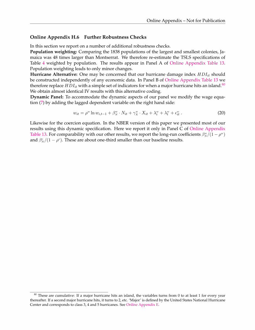
Online Appendix – Not for Publication

Online Appendix H.6 Further Robustness Checks

In this section we report on a number of additional robustness checks.Population weighting: Comparing the 1838 populations of the largest and smallest colonies, Ja-maica was 48 times larger than Montserrat. We therefore re-estimate the TSLS specifications ofTable 4 weighted by population. The results appear in Panel A of Online Appendix Table 13.Population weighting leads to only minor changes.Hurricane Alternative: One may be concerned that our hurricane damage index HDIit shouldbe constructed independently of any economic data. In Panel B of Online Appendix Table 13 wetherefore replaceHDIit with a simple set of indicators for when a major hurricane hits an island.80

We obtain almost identical IV results with this alternative coding.Dynamic Panel: To accommodate the dynamic aspects of our panel we modify the wage equa-tion (7) by adding the lagged dependent variable on the right hand side:

wit = ρw lnwi,t−1 + βwN ·Nit + γwX ·Xit + λwi + λwt + εwit . (20)

Likewise for the coercion equation. In the NBER version of this paper we presented most of ourresults using this dynamic specification. Here we report it only in Panel C of Online AppendixTable 13. For comparability with our other results, we report the long-run coefficients βwN/(1− ρw)and βcN/(1− ρc). These are about one-third smaller than our baseline results.

80 These are cumulative: If a major hurricane hits an island, the variables turns from 0 to at least 1 for every yearthereafter. If a second major hurricane hits, it turns to 2, etc. ‘Major’ is defined by the United States National HurricaneCenter and corresponds to class 3, 4 and 5 hurricanes. See Online Appendix E.

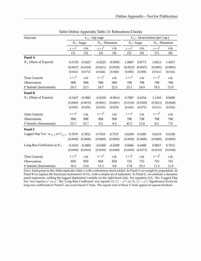
Online Appendix – Not for Publication

Table Online Appendix Table 13: Robustness Checks

Outcome w it : log wage C it : Incarceration (per Cap.)

t + t2 t-fe t + t2 t-fe t + t2 t-fe t + t2 t-fe

(1) (2) (3) (4) (5) (6) (7) (8)

Panel AN it (Share of Exports) -0.5729 -0.5627 -0.9225 -0.9595 1.0847 0.8771 1.6613 1.4357

[0.0067] [0.0104] [0.0021] [0.0029] [0.0022] [0.0047] [0.0005] [0.0003]

{0.043} {0.071} {0.044} {0.068} {0.006} {0.009} {0.011} {0.016}

Time Controls t + t2t-fe t + t2

t-fe t + t2t-fe t + t2

t-fe

Observations 908 908 908 908 798 798 798 798

F Statistic (Instruments) 24.2 22.1 24.7 22.5 23.1 24.4 19.5 21.9

Panel BN it (Share of Exports) -0.5437 -0.5881 -0.8359 -0.9614 0.7887 0.6354 1.1343 0.9499

[0.0069] [0.0076] [0.0001] [0.0001] [0.0150] [0.0309] [0.0012] [0.0048]

{0.059} {0.059} {0.033} {0.029} {0.042} {0.075} {0.011} {0.036}

Time Controls t + t2t-fe t + t2

t-fe t + t2t-fe t + t2

t-fe

Observations 908 908 908 908 798 798 798 798

F Statistic (Instruments) 55.7 52.7 9.2 8.4 45.5 51.8 8.2 7.9

Panel CLagged Dep Var: w i,t -1 or C i,t -1 0.7679 0.7652 0.7610 0.7537 0.6294 0.6385 0.6219 0.6328

[0.0000] [0.0000] [0.0000] [0.0000] [0.0000] [0.0000] [0.0000] [0.0000]

Long-Run Coefficient on N it -0.4316 -0.3865 -0.6360 -0.6209 0.6666 0.4480 0.9827 0.7015[0.0448] [0.0416] [0.0394] [0.0448] [0.0204] [0.0372] [0.0233] [0.0346]

Time Controls t + t2t-fe t + t2

t-fe t + t2t-fe t + t2

t-fe

Observations 859 859 859 859 725 725 725 725

F Statistic (Instruments) 16.5 15.6 12.2 9.8 17.8 19.3 11.5 11.9

N it : Sugar N it : Plantation N it : Sugar N it : Plantation

Notes: Each panel in this Table replicates Table 4 with a robustness check added. In Panel A we weight by population. InPanel B we replace the hurricane instrument HDIit with a simple set of indicators. In Panel C, we estimate a dynamicpanel regression, adding the lagged dependant variable on the right-hand side. See equation (20). The ‘Lagged DepVar’ row reports ρw or ρc. The ‘Long-Run Coefficient’ row reports βwN/(1 − ρw) or βcN/(1 − ρc). Significance levels forlong-run coefficients in Panel C use score-based F tests. The square root of these F -tests appear in square brackets.

Online Appendix – Not for Publication

Online Appendix I Extensions

Extension I: Dispensing with Nit altogether and instead instrumenting coercion Cit with Oit,we obtain the causal effect of outside-option-reducing coercion on wages under the assumptionthat Oit impacts wit only through Cit:

wit = βWC · Cit + γWX ·Xit + λWi + λWt + εWit , (21)

whereCit is instrumented withOit. The associated first-stage equation is exactly the reduced-formrelation in equation (11), which is reported in columns 7–8 of Table 3. Similarly, the reduced-formequation corresponding to (21) is the same as equation (10), which is reported in columns 5–6 ofTable 3. Online Appendix Table 14 reports the results of estimating (21) using IV. The number ofobservations for which we observe both Cit and wit is 750. In both specifications, the results implythat an increase in incarceration rates of about one person per hundred in a year (slightly less thanthe mean incarceration rate in the data) decreases wages by about sixty percent. This is consistentwith the results reported in Table 4, where the estimated coefficient of the declining plantationssystem on wit was about sixty percent of that on Cit (i.e., −.05736 in columns 2 over 0.8869 incolumn 6 of Table 4).

Online Appendix – Not for Publication

Table Online Appendix Table 14: IV Effect of Coercion (Cit) on Wages (wit)

Outcome w it : log wage

(1) (2)

C it : Incarceration (per Cap.) -0.5427 -0.6535

[0.0008] [0.0003]

{0.046} {0.022}

Time Controls t + t2t-fe

Observations 750 750

F Statistic (Instruments) 23.762 14.751

Notes: (a) This table reports on the IV results of estimating equation (21). 750 is the number of observations for whichwe observe both Cit and wit. All controls that were included columns 2, and 4 in Table 1 are also included here. Thefirst-stage relation corresponding to above results is that reported in columns 7–8 of Table 3. (b) Standard errors areclustered by colony, p-values in square brackets; p-values for wild-bootstrapped standard errors are shown in curlybrackets.

Online Appendix – Not for Publication

Extension II: Instead of dispensing with Nit, we now take the opposite direction by attemptingto estimate what portion of the effect of Nit on wit works through Cit and what portion affects wit‘directly’ (i.e., through other channels). A decomposition like this is done through a ‘mediationanalysis,’ which asks to what extent the ‘total effect’ of a treatment variable (e.g. Nit) on a ‘finaloutcome’ (e.g. wit) is explained by an intermediate outcome or mechanism (e.g. Cit) that is alsoan outcome of Nit. See for example Imai et al. (2010, 2011); Heckman et al. (2013); Heckman andPinto (2015b). We fix ideas using Online Appendix Figure 9. The Base-Model in Online AppendixFigure 9 represents the IV estimations reported in Table 4 of Section 4. In them, the relationshipbetween Nit and the outcomes Cit and wit is confounded by unobservables (the V ), but Oit is bothplausibly independent of these unobservables and a powerful predictor of Nit, thus constitutinga valid instrument. Extension I in Online Appendix Figure 9 disregards Nit altogether and insteaduses Oit as an instrument for Cit on wit. Extension II applies a mediation analysis to this IV setting.Under certain assumptions, Extension II can be estimated using just the instruments at hand andwe can ask to what extent the plantation system reduced wages because it raised coercion.81

It is important to note that Extension I and Extension II are both consistent with the standardIV identification assumptions of the Base-Model in Section 4. However, Extension I and Extension IIare not consistent with each other. This is because Oit can only be a valid instrument in Extension Iunder the exclusion restriction that it impacts wit only through Cit, which is the assumption that isbeing relaxed in Extension II. Extension I and Extension II should therefore be viewed as extendingthe empirical analysis from Section 4 into different directions, by making different assumptionsabout unobservables.

81 Without additional dedicated instruments for Cit, identification in Extension II requires that confounders that biasthe relationship between Nit and wit work only through Cit. In other words, the relationship between the plantationsystem and wages is biased only because of confounders that impact wages through coercion. While it is a strong as-sumption that there are no unobservables that directly impacted wages and the plantation system, it is not implausiblegiven that we control for all historically prominent labor demand and supply shocks during this period.

Online Appendix – Not for Publication

Figure Online Appendix Figure 9: Extending the AnalysisTable 1: General Mediation Model and Our Solution to the Identification Problem

A. Directed Acyclic Graph (DAG) Representation

Base-Model: Extension I: Extension II:

IV for N → C,W IV for C →W IV Mediation Model

V

N C,WO

V ′

C WO

V

N C W

V ′

O

B. Structural Equations

N = fN (O, V, εN ),

C = fC(N,V, εC),

W = fW (N,V, εW ),

O,V, ε′s Stat. Indep.

C = fC(O, V ′, εC),

W = fW (C, V ′, εW ),

O,V ′, ε′s Stat. Indep.

N = fN (O, V, εN )

C = fC(N,V, V ′, εC)

W = fW (N,C, V ′, εW )

O,V, V ′, ε′s Stat. Indep.

The first column of Panel A gives the DAG representation of the two IV Models, which enable the identification of thecausal effects of T on M and Y . The third column of Panel A presents the General Mediation Model with an instru-mental variable Z. In the third column, identification can only be achieved with an additional designated instrumentfor M (not depicted). The fourth column of Panel A presents the Restricted Mediation Model with an instrumentalvariable Z. This model enables the identification of the total, the direct and the indirect effect of T on Y. The modelalso enables the identification of the causal effect of T on M as well as the causal effect of M on Y. Panel B presentsthe nonparametric structural equations of each model. Conditioning variables are suppressed for sake of notationalsimplicity. U , discussed in the text, is included in the equations but omitted from the DAGs for expositional clarity.The full DAGs, which include U , are in section ??. We refer to Heckman and Pinto (2015a) for a recent discussion oncausality and directed acyclic graphs.

“The fact that the wage level in the capitalist sector depends upon earnings in the

subsistence sector is of immense political importance, since its effect is that capitalists

have a direct interest in holding down the productivity of the subsistence workers.

Thus the owners of plantations, if they are influential in the government, are often

found engaged in turning the peasants off their lands.” — Lewis (1954)

1 Introduction

Many economists and historians would agree with Acemoglu and Wolitzky’s 2011 assessment

that “the majority of labor transactions throughout much of history and a significant fraction of

such transactions in many developing countries today are coercive”. Indeed, labor coercion is at

the heart of much of the literature on long run development and institutional change (Domar,

1

Notes: The first column of Panel A, labeled the Base-Model, gives the Directed Acyclic Graphs (DAG) representation ofthe two IV estimations in section 4. Extension I is the IV model where C is instrumented directly with O. Extension IIis an IV Mediation Model that allows for the identification of the causal effect of N on W as it is mediated by coercionC. Extension I and Extension II are both consistent with the identification assumptions of the Base-Model. However,Extension I and Extension II are not consistent with each other: O can only be a valid instrument for C in Extension Iunder the exclusion restriction that it impactsW only through C. Panel B presents the nonparametric equations of eachmodel. We refer to Heckman and Pinto (2015a) for a recent discussion on causality and DAGs.

Online Appendix – Not for Publication

We estimate Extension II using the following equation

wit = βw|NC · Cit + βw|NN ·Nit + γw|NX ·Xit + λw|Ni + λw|Nt + εw|Nit . (22)

Equation (22) allows coercion to affect wages (βw|NC < 0) and allows the plantation system to affectwages through channels other than coercion (βw|NN 6= 0). It cannot be estimated by OLS when Nit

and Cit are endogenous. However, Pinto et al. (2019) show that (22) can be estimated using IV,as long as the assumptions on the error term that are laid out in Extension II of Online AppendixFigure 9 hold. In that case, the causal effect of Cit on wit can be estimated by instrumenting for Citwith Oit while including Nit in both the second-stage and first-stage equations.82

An intuition for the identifying variation in Extension II can be gained by observing that con-ditional on Nit, the unobserved confounder V is in principle an instrument for Cit in Extension IIbecause it enters the system only through Cit. Furthermore, although Oit has to be uncorrelatedwith V (in order to have been a valid instrument in the Base-Model), this need not be true once wecondition on Nit, an insight that is basically an application of Simpson’s Paradox.83

To identify the causal effect of Cit on wit in Extension II, we estimate equation (22) using IV. Theresulting estimate βw|NC in Online Appendix Table 15 suggests that when the plantation systemincreased incarcerations by one person per hundred this lowered agricultural wages by between30-40 percent (e.g. −0.33 = e−0.4070 − 1 in column 1).

The question that is ultimately posed in Extension II is how much of the effect of Nit on wit isexplained by the effect of Nit on Cit. To answer it, we need only combine βw|NC from equation (22)with βCN and βwN , the coefficient estimates from equations (7) and (8), which we reported in Table 4.The share of the effect of Nit on wit that operates via coercion Cit is defined as (βCN × βw|NC )/βwN .This share is reported at the bottom of Online Appendix Table 15. For example, we estimatedβwN = −0.5736 and βCN = 0.8869 in columns 2 and 6 of Table 4. Combining this with the estimateof βw|NC in column 2 of Online Appendix Table 15, we get 0.856 = (0.8869 × .0.5496)/(−0.5736).Across specifications, this type of calculation suggests that between 75 and 90 percent of the effectof the declining plantation system on rising wages wit operates via lowered coercion as measuredby Cit.

Summarizing the additional insights gleaned in this section, Extension II makes stronger iden-tifying assumptions than Extension I but also sheds additional light on the workings of coercion,enabling us to uncover evidence that is consistent with the motivating quote by Lewis (1954).Further, while Extension I and Extension II make different identifying assumptions, the evidencegenerated by the two models is nonetheless highly consistent: Extension I, which assumes that Oitimpacts wages only through measured coercion Cit, implies that an increase in incarceration ratesof one person per hundred in a year decreases wages by about 55–65 percent. Extension II, whichallows Oit to impacts wages through channels other than Cit, implies that this same increase in

82 The first-stage equation is

Cit = βC|NO ·Oit + β

C|NN ·Nit + γ

C|NX ·Xit + λ

C|Ni + λ

C|Nt + ε

C|Nit . (23)

83 For example, suppose that—as we argued in footnote 38 — the unmeasured influence of local missionaries is agood candidate for V . Missionaries fostered resistance against the plantation system, thereby increasing incarcerationsCit and depressing Nit, potentially leading to downward-biased OLS estimates for equation (8). While the unobservedpresence of missionaries is assumed to be uncorrelated with Oit, a high residual value of Oit conditional on Nit may infact imply a low presence of missionaries, and should therefore cause lower incarceration rates. This is because observ-ing a high natural ability to evade the plantation system given its observed strength Nit is the same as a ‘surprisingly’strong plantation system given the natural ability to evade it. We refer to Dippel, Gold, Heblich and Pinto (2017) for adetailed treatment and proofs. Whether Oit in fact has a significant impact on Cit conditional on Nit is an empiricalquestion of instrument power, not an econometric question of instrument validity.

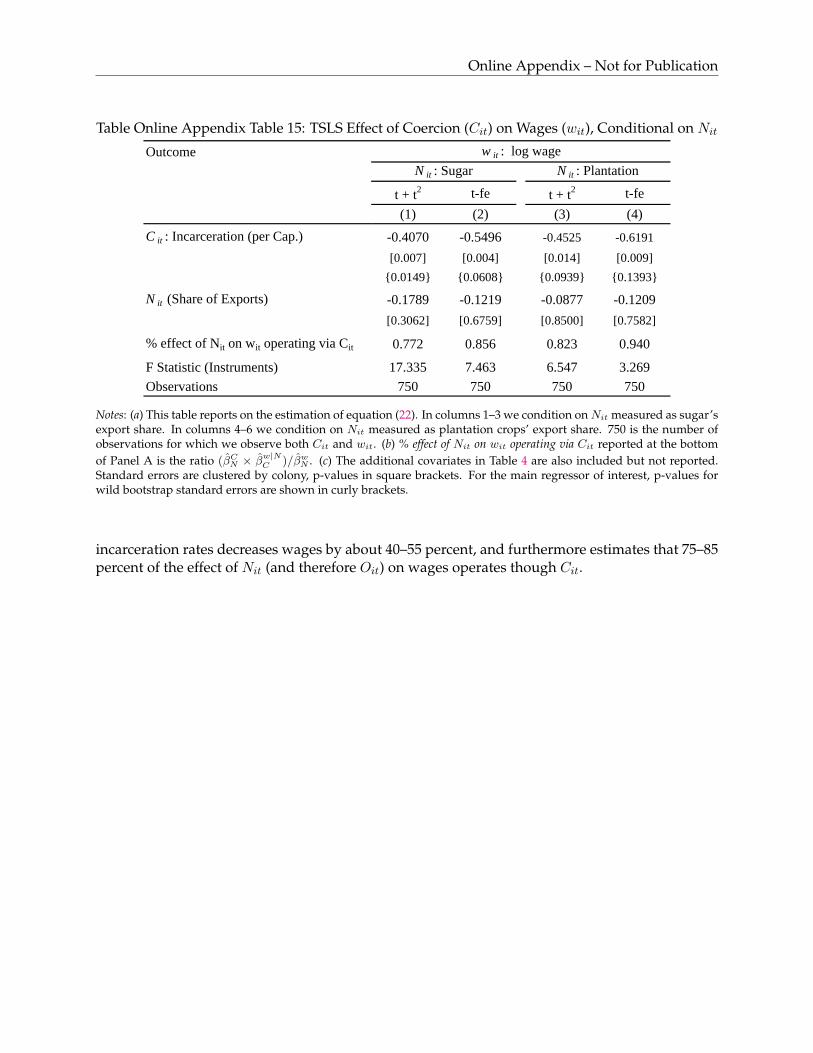
Online Appendix – Not for Publication

Table Online Appendix Table 15: TSLS Effect of Coercion (Cit) on Wages (wit), Conditional on Nit

Outcome w it : log wage

t + t2 t-fe t + t2 t-fe

(1) (2) (3) (4)

C it : Incarceration (per Cap.) -0.4070 -0.5496 -0.4525 -0.6191

[0.007] [0.004] [0.014] [0.009]

{0.0149} {0.0608} {0.0939} {0.1393}

N it (Share of Exports) -0.1789 -0.1219 -0.0877 -0.1209

[0.3062] [0.6759] [0.8500] [0.7582]

% effect of Nit on wit operating via Cit 0.772 0.856 0.823 0.940

F Statistic (Instruments) 17.335 7.463 6.547 3.269

Observations 750 750 750 750

N it : Sugar N it : Plantation

Notes: (a) This table reports on the estimation of equation (22). In columns 1–3 we condition onNit measured as sugar’sexport share. In columns 4–6 we condition on Nit measured as plantation crops’ export share. 750 is the number ofobservations for which we observe both Cit and wit. (b) % effect of Nit on wit operating via Cit reported at the bottomof Panel A is the ratio (βCN × β

w|NC )/βwN . (c) The additional covariates in Table 4 are also included but not reported.

Standard errors are clustered by colony, p-values in square brackets. For the main regressor of interest, p-values forwild bootstrap standard errors are shown in curly brackets.

incarceration rates decreases wages by about 40–55 percent, and furthermore estimates that 75–85percent of the effect of Nit (and therefore Oit) on wages operates though Cit.

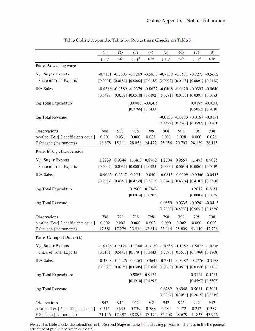
Online Appendix – Not for Publication

Table Online Appendix Table 16: Robustness Checks on Table 5

(1) (2) (3) (4) (5) (6) (7) (8)

t + t2 t-fe t + t2 t-fe t + t2 t-fe t + t2 t-fe

Panel A: w it , log wage

N it : Sugar Exports -0.7151 -0.5683 -0.7269 -0.5658 -0.7138 -0.5671 -0.7275 -0.5662

Share of Total Exports [0.0004] [0.0181] [0.0002] [0.0158] [0.0002] [0.0163] [0.0001] [0.0148]

IEA Salesit -0.0388 -0.0589 -0.0379 -0.0627 -0.0408 -0.0620 -0.0393 -0.0640

[0.0495] [0.0258] [0.0518] [0.0092] [0.0281] [0.0173] [0.0391] [0.0083]

log Total Expenditure 0.0083 -0.0305 0.0195 -0.0200

[0.7766] [0.5433] [0.5052] [0.7010]

log Total Revenue -0.0133 -0.0183 -0.0167 -0.0151

[0.4429] [0.2398] [0.3592] [0.3203]

Observations 908 908 908 908 908 908 908 908

p-value: Test[ 2 coefficients equal] 0.001 0.031 0.000 0.028 0.001 0.028 0.000 0.026

F Statistic (Instruments) 18.878 15.111 28.058 24.472 25.056 20.703 28.129 26.115

Panel B: C it , Incarceration

N it : Sugar Exports 1.2239 0.9346 1.1463 0.8962 1.2304 0.9557 1.1495 0.9025

Share of Total Exports [0.0001] [0.0031] [0.0001] [0.0025] [0.0000] [0.0030] [0.0001] [0.0019]

IEA Salesit -0.0662 -0.0547 -0.0551 -0.0404 -0.0613 -0.0509 -0.0566 -0.0433

[0.2909] [0.4050] [0.4239] [0.5612] [0.3246] [0.4394] [0.4107] [0.5360]

log Total Expenditure 0.2500 0.2343 0.2682 0.2651

[0.0014] [0.0202] [0.0003] [0.0035]

log Total Revenue 0.0559 0.0335 -0.0241 -0.0413

[0.2380] [0.5763] [0.5651] [0.4559]

Observations 798 798 798 798 798 798 798 798

p-value: Test[ 2 coefficients equal] 0.000 0.002 0.000 0.002 0.000 0.002 0.000 0.002

F Statistic (Instruments) 17.581 17.279 33.914 32.816 33.944 35.809 43.140 47.738

Panel C: Import Duties (£)

N it : Sugar Exports -1.0126 -0.6124 -1.7386 -1.3130 -1.4885 -1.1082 -1.8472 -1.4236

Share of Total Exports [0.3102] [0.5148] [0.1791] [0.3043] [0.2095] [0.3577] [0.1709] [0.2808]

IEA Salesit -0.3593 -0.4226 -0.3263 -0.3645 -0.2811 -0.3287 -0.2776 -0.3168

[0.0026] [0.0298] [0.0305] [0.0858] [0.0068] [0.0639] [0.0350] [0.1161]

log Total Expenditure 0.9063 0.9131 0.5184 0.4231

[0.3910] [0.4292] [0.4597] [0.5507]

log Total Revenue 0.6282 0.6968 0.5081 0.5991

[0.3067] [0.3054] [0.2615] [0.2619]

Observations 942 942 942 942 942 942 942 942

p-value: Test[ 2 coefficients equal] 0.515 0.835 0.239 0.388 0.284 0.472 0.212 0.337

F Statistic (Instruments) 21.146 17.397 38.895 37.474 32.708 28.679 41.823 43.956

Notes: This table checks the robustness of the Second Stage in Table 5 to including proxies for changes in the the generalstructure of public finance in our data.

Online Appendix – Not for Publication

Table Online Appendix Table 17: The Effect of the IEA

Outcome N it : Plantations'

Export ShareN it : Sugar's Export

ShareIEA Salesit

Time Controls t + t2t-fe t + t2

t-fe t + t2t-fe

(1) (2) (3) (4) (5) (6)

Panel A

O i x English Exports -0.2294 -0.2243 -0.4259 -0.4684 0.0571 0.1145

to all Non-Caribbeant [0.0095] [0.0033] [0.0001] [0.0001] [0.5714] [0.3641]

HDIit -0.0643 -0.0642 -0.0635 -0.0672 0.0086 0.0150

[0.0000] [0.0000] [0.0000] [0.0000] [0.3880] [0.2596]

Incumbered Estate Act (IEA) -0.0187 -0.0168 -0.0059 -0.0088 1.0386 1.0538

Petitionsit [0.2593] [0.3811] [0.7967] [0.7396] [0.0000] [0.0000]

Observations 942 942 942 942 942 942

R-squared 0.882 0.884 0.895 0.901 0.990 0.990

Panel B

O i x English Exports -0.2414 -0.2453 -0.4419 -0.4978 -0.0137 0.0264

to all Non-Caribbeant [0.0094] [0.0042] [0.0001] [0.0001] [0.7642] [0.5696]

HDIit -0.0591 -0.0590 -0.0594 -0.0634 0.0004 0.0048

[0.0000] [0.0000] [0.0000] [0.0000] [0.9085] [0.2031]

Incumbered Estate Act (IEA) -0.0251 -0.0227 -0.0126 -0.0162 1.0479 1.0592

Petitionsit [0.3103] [0.3850] [0.6730] [0.5991] [0.0000] [0.0000]

Observations 908 908 908 908 908 908

R-squared 0.889 0.891 0.897 0.904 0.995 0.995

Panel C

O i x English Exports -0.2342 -0.2430 -0.4421 -0.4942 -0.0242 0.0094

to all Non-Caribbeant [0.0176] [0.0119] [0.0002] [0.0002] [0.5413] [0.8245]

HDIit -0.0585 -0.0590 -0.0575 -0.0616 0.0005 0.0049

[0.0000] [0.0000] [0.0000] [0.0000] [0.8856] [0.2707]

Incumbered Estate Act (IEA) -0.0180 -0.0149 -0.0052 -0.0089 1.0458 1.0570

Petitionsit [0.3211] [0.4716] [0.8167] [0.7204] [0.0000] [0.0000]

Observations 798 798 798 798 798 798

R-squared 0.891 0.895 0.904 0.912 0.995 0.995

Notes: This table re-reports the First Stage in Table 5 for the 3 different numbers of observations in that table’s Panel A.

Online Appendix – Not for Publication

References

American and Foreign Anti-Slavery Society, The Annual Report of the American and Foreign Anti-Slavery Society Presented at New York ... with the Addresses and Resolutions, New York: Americanand Foreign Anti-Slavery Society, 1849.

Bekele, Frances L., “The History of Cocoa Production in Trinidad and Tobago,” in L.A. Wilson,ed., Re-vitalisation of the Trinidad & Tobago Cocoa Industry: Proceedings of the APASTT Seminar,Trinidad and Tobago: Association of Professional Agricultural Scientists of Trinidad and To-bago, 2004, pp. 4–12.

Berland, Alexander J., Sarah E. Metcalfe, and Georgina H. Endfield, “Documentary-derivedChronologies of Rainfall Variability in Antigua, Lesser Antilles, 1770-1890,” Climate of the Past,2013, 9 (3), 1331–1343.

Brizan, George I., Grenada, Island of Conflict: from Amerindians to People’s Revolution, 1498-1979,London: Zed Books, 1984.

Carvalho, Jean Paul and Christian Dippel, “Elite Identity and Political Accountability: A Tale ofTen Islands,” Technical Report, NBER Working Paper 22777 2016.

Craig-James, Susan, The Social and Economic History of Tobago (1838–1990): Persistent Poverty in theAbsence of Adequate Development Strategy, Tobago, Scarborough: PRDI, 2000.

Deerr, Noel, The History of Sugar, London: Chapman and Hall, 1950.

Dookhan, Isaac, A History of the British Virgin Islands, 1672–1970, Epping, England: CaribbeanUniversities Press, 1975.

Eisner, Gisela, Jamaica, 1830-1930: A Study in Economic Growth, Manchester: Manchester Univer-sity Press, 1961.

Eltis, David, Frank D. Lewis, and David Richardson, “Slave Prices, the African Slave Trade, andProductivity in the Caribbean, 1674–1807,” The Economic History Review, 2005, 58 (4), 673–700.

Engerman, Stanley L., “Economic Change and Contract Labor in the British Caribbean: The Endof Slavery and the Adjustment to Emancipation,” Explorations in Economic History, 1984, 21 (2),133–150.

and Kenneth L. Sokoloff, “Factor Endowments, Institutions, and Differential Paths of GrowthAmong New World Economies: A View from Economic Historians of the United States,” inStephen Harber, ed., How Latin America Fell Behind, Stanford: Stanford University Press, 1997,pp. 260–304.

Fergus, Howard A., Montserrat: History of a Caribbean Colony, Hong Kong: Macmillan Caribbean,1994.

Online Appendix – Not for Publication

Froude, James Anthony, The English in the West Indies: Or, The Bow of Ulysses, London: Longmans,Green, 1888.

Gibson, Campbell and Kay Jung, Historical census statistics on population totals by race, 1790 to 1990,and by Hispanic origin, 1970 to 1990, for large cities and other urban places in the United States, U.S.Census Bureau, 2005.

Great Britain, The Colonial Blue Book for the Leewards Islands, London: H.M.’s Stationery Office,1911.

Green, William A., British Slave Emancipation: The Sugar Colonies and the Great Experiment 1830-1865, Oxford: Clarendon Press, 1976.

Hall, Douglas, Five of the Leewards: 1834–1870, Epping, England: Caribbean Universities Press,1971.

Handler, Jerome S., “The History of Arrowroot Production in Barbados and the Chalky MountArrowroot Growers’ Association, a Peasant Marketing Experiment that Failed,” Journal of theBarbados Museum and Historical Society, 1965, 31 (3), 1–22.

, “The History of Arrowroot and the Origin of Peasantries in the British West Indies,” Journal ofCaribbean History, May 1971, 2, 46–93.

Harmsen, Jolien, Guy Ellis, and Robert J. Devaux, A History of St Lucia, Vieux Fort, St Lucia:Lighthouse Road Publications, 2012.

Harrigan, Norwell and Pearl Varlack, The Virgin Islands Story, Epping, England: Caribbean Uni-versities Press, 1975.

Heckman, James J. and Rodrigo Pinto, “Causal Analysis after Haavelmo,” Econometric Theory,2015, 31 (1), 115–151.

Heckman, James J and Rodrigo Pinto, “Econometric Mediation Analyses: Identifying the Sourcesof Treatment Effects from Experimentally Estimated Production Technologies with Unmeasuredand Mismeasured Inputs,” Econometric Reviews, 2015, 34 (1-2), 6–31.

Heckman, James J., Rodrigo Pinto, and Peter A. Savelyev, “Understanding the MechanismsThrough Which an Influential Early Childhood Program Boosted Adult Outcomes,” AmericanEconomic Review, 2013, 103 (6), 2052–2086.

Higman, Barry W., “The Sugar Revolution,” Economic History Review, 2000, 53 (2), 213–236.

Imai, Kosuke, Luke Keele, and Te Yamamoto, “Identification, Inference and Sensitivity Analysisfor Causal Mediation Effects,” Statistical Science, 2010, 25 (1), 51–71.

Online Appendix – Not for Publication

, , Dustin Tingley, and Teppei Yamamoto, “Unpacking the Black Box of Causality: Learningabout Causal Mechanisms from Experimental and Observational Studies,” American PoliticalScience Review, 2011, 105 (4), 765–789.

Jacks, David S., “Intra- and International Commodity Market Integration in the Atlantic Economy,1800–1913,” Explorations in Economic History, 3 2005, 42, 381–413.

Jayasinghe, P.K.S.C. and Masao Yoshida, “Development of Two GIS-based Modeling Frame-works to Identify Suitable Lands for Sugarcane Cultivation,” Tropical Agriculture and Develop-ment, 2010, 54 (2), 51–61.

Knapp, Arthur W., Cocoa and Chocolate: Their History from Plantation to Consumer, London: Chap-man and Hall, 1920.

Lewis, Gordon K., The Growth of the Modern West Indies, New York: Monthly Review Press, 1986.

Lewis, W Arthur, “Economic Development with Unlimited Supplies of Labour,” The ManchesterSchool, 1954, 22 (2), 139–191.

Martin, Robert M., Statistics of the Colonies of the British Empire, London: WH Allen and Company,1839.

Merivale, Herman, Lectures on Colonization and Colonies, London: Longman, Green and Roberts,1861.

Nugent, Jeffrey B and James A Robinson, “Are Factor Endowments Fate?,” Journal of Iberian andLatin American Economic History, 2010, 28, 45–82.

Pinto, R., C. Dippel, R. Gold, and S. Heblich, “Mediation Analysis in IV Settings With a SingleInstrument,” 2019.

Richardson, Bonham C., Economy and Environment in the Caribbean: Barbados and the Windwards inthe Late 1800s, Mona, Jamaica: University of the West Indies Press, 1997.

Sewell, William G., The Ordeal of Free Labor in the British West Indies, Harper & brothers, 1861.

Sokoloff, Kenneth L. and Stanley L. Engerman, “History Lessons: Institutions, Factor Endow-ments, and Paths of Development in the New World,” Journal of Economic Perspectives, 2000, 14(3), 217–232.

Soluri, John, “Bananas Before Plantations. Smallholders, Shippers, and Colonial Policy in Jamaica,1870–1910,” Iberoamericana, 2006, 6 (23), 143–159.

Tannehill, Ivan Ray, Hurricanes: Their Nature and History: Particularly those of the West Indies andthe Southern Coasts of the United States, Princeton: Princeton University Press, 1938.

Trouillot, Michel-Rolph, Peasants and Capital: Dominica in the World Economy, Baltimore: JohnsHopkins University Press, 1988.

United States National Hurricane Center, “NHC Data Archive,” October 2014. Retrieved October2013.

50