output persistence, economic structure, and the choice of

STEVEN N. DURLAUF Stanford University

Output Persistence, Economic

Structure, and the Choice of

Stabilization Policy

A STRIKING change in empirical macroeconomics in the 1980s has been the development of an alternative way to think about aggregate trends and cycles. Traditionally, aggregate series such as gross national product have been modeled as stationary processes about a deterministic trend. All aggregate fluctuations were thus short-run phenomena with no bearing on the long-run behavior of the economy. Starting with the work of Charles Nelson and Charles Plosser, however, empirical workers have developed considerable evidence that suggests that some component of aggregate activity follows a stochastic trend-the long-run path of the macroeconomy is permanently affected by contemporary events. I

This perspective means that not only are trend-cycle decompositions extremely difficult, in that the same structural stochastic elements affect both underlying time series, but that, in addition, the feedback mechanisms from current activity to long-run growth render the traditional distinction meaningless.

The identification of unit roots has become a veritable cottage industry among empirical workers. On the other hand, there has been comparatively little work on the economics of unit roots. Most theoretical work on the subject has treated unit roots exclusively as a manifestation of

I thank Andrew Bernard, Robert Hall, David Romer, John Shoven, Christopher Sims, Gavin Wright, and members of the Brookings Panel for helpful discussions. Outstanding research assistance by Andrew Bernard and Suzanne Cooper is gratefully acknowledged. Laura Dolly has supplied superb secretarial support. All errors are mine.

1. Nelson and Plosser (1982). 69

70 Brookings Papers on Economic Activity, 2:1989

technology or supply shocks. Robert King and others assume that the persistent component of GNP is generated by a random walk in technology.2 Jones and Manuelli show that if the marginal product of capital is bounded sufficiently above zero, stationary innovations to wealth will be spread over an infinite horizon.3 This idea is of course the basis of the random walk theory of consumption, which requires that the gross marginal product of capital is a constant equal to the inverse of the discount rate. These examples, however, require very specialized assumptions on technology. Typically, macroeconomists employ representative agent models to explain the behavior of aggregate time series. This class of models represents the equilibrium sample path for the economy as the solution to some sort of dynamic programming problem. Dynamic programming problems in turn generate unit roots in control variables only for isolated parameter values unless one assumes that some of the exogenous state variables already contain unit roots. From the representative agent perspective, unit roots are rare phenomena. Christopher Sims has gone so far as to conclude that the theoretical justification for looking for unit roots follows from "algebraic conven- ience and professional inertia, not by experimental evidence or intuitive plausibility." 4

Interest in the existence of unit roots has been matched by interest in assessing the role of permanent shocks in explaining total fluctuations. Aggregate fluctuations may be conceptualized as generated by a combination of persistent and mean-reverting components. The importance of the unit root as a contributor to the variance of output changes has engendered considerable controversy. John Campbell, N. Gregory Mankiw, and John Cochrane have developed substantially different perspectives on the magnitude of the unit root component of GNP.' The unit root has further been treated by numerous authors as a measure of the component of aggregate innovations induced by supply-side factors. Olivier Blanchard and Danny Quah perform trend-cycle decompositions by assuming that demand shocks are transitory.6 J. Bradford De Long and Lawrence Summers go so far as to argue that the greater persistence

2. King and others (1987). 3. Jones and Manuelli (1987). 4. Sims (1988, p. 464). 5. Campbell and Mankiw (1987a); Cochrane (1988). 6. Blanchard and Quah (1988).

Steven N. Durlauf 71

in postwar than pre-Depression fluctuations is proof that stabilization policy has been a success, on the grounds that successful policy can eliminate only mean-reverting fluctuations.i

This paper considers the role of unit root findings in the interpretation of economic fluctuations and in the formulation of monetary and fiscal policy rules. The paper complements Sims's critique in the sense that it emphasizes that what is important about output fluctuations is persistence rather than the presence of an exact unit root. In several respects, exact unit root findings may not even matter. First, from the vantage point of a social planner, exact and near unit roots are equivalent. Intuitively, a social welfare function that discounts future utility is unaffected by distant events, so that permanence of innovations is not necessarily important. Second, unit roots provide little information for identifying economic structure. This claim follows from several considerations. Empirically, cross-country data provide little evidence that permanent shocks eventually migrate internationally, whereas many sectors of the American economy seem to possess a common unit root despite differences in production functions. On the theoretical side, various business cycle models with fundamentally different policy implications may be shown to be compatible with unit roots in economic time series.

Although thus rejecting some previous interpretations of the data, this paper argues that the unit root evidence is important in several senses. Unit roots represent a parsimonious way of expressing the persistence of fluctuations and as such are a significant stylized fact about the macroeconomy. This stylized fact is a natural implication of dynamic coordination failure and is therefore consistent with much current macroeconomic theory. Understanding the degree of persistence in aggregate fluctuations helps in assessing the potential role of coordination failure as a source of fluctuations.

Further, understanding the degree of persistence in economic fluctuations is essential for computing welfare-maximizing policy rules. The divided state of empirical and theoretical macroeconomics means that a policymaker ought to be modeled as uncertain about economic structure. Uncertainty about economic structure is equivalent in this context to uncertainty about policy effects-a question originally analyzed by

7. De Long and Summers (1988).


William Brainard.8 Brainard's work demonstrated that when policy multipliers are random, optimal policy construction leads to a diversification of countercyclical policy choices. Brainard's original research concentrated on the role of multiple policy instruments in diversifying the uncertainty of individual policies. In the case of uncertain structure and one policy instrument, this idea can be exploited to demonstrate that one chooses a rule that weights the optimal rules under each structure based upon minimizing some expected value function. The optimal rule diversifies in the sense that it constructs a weighting across different rules that are each optimal, conditional on a given regime.

Persistence in fluctuations means that if stabilization policy successfully reverses downturns, then the social welfare improvements are very large. As a result, the new empirical macroeconomics places a large weight on a countercyclical policy rule. Consequently, persistence in output leads to powerful policy implications even in the absence of strong implications about economic structure.9

Welfare and Persistence

The issue of unit roots and output persistence centers on long-run forecasts of log per capita output Yt. In traditional formulations

cc

(1) yt = Pt + E wjEt-j j=0

where t denotes time and the E's are white noise innovations. In this formulation, the y coefficients are square summable, j%=o -yj2 < X, which in turn implies that the weights yj decline to zero.

When output can be represented in this fashion, then long-run forecasts of GNP eventually become independent of the history of the process:

(2) lim E(Yk - IkIEt) = 0.

8. Brainard (1967). 9. In fact, the "new macroeconomics" articulated by Robert Hall and others, where

the aggregate equilibrium is indeterminate, leads to similar policy conclusions. See Hall (1989) for an example of this type of model.


Likewise, (3) lim EL Yk - 3kILY(t)] = O,

k=>oc

where Ly(t) represents total information contained in linear combinations of Yt, Yt 1-. . . . In the traditional perspective, the deterministic trend, by proxying for technical change, captures the long-run dynamics of the economy.

The new perspective on aggregate behavior treats the changes in output as a stationary process. The canonical form for the time series of output changes is

cc

(4) A Yt + Oj Et j j= 0

where the a- coefficients are square summable and the innovations E are uncorrelated with zero mean. Since one can think of YK, as Yt + EJ=1

A Y,+j, the long-run forecast of the economy is affected by the expectations of all future changes in output. If there is no tendency for shocks to the economy to revert to zero, then it is apparent that history matters for long-run predictions about the economy. 10

Persistence in aggregate output reveals nothing about its relative importance as a component of fluctuations. This is true in two senses. First, there is a statistical question as to the magnitude of persistence as a component of total fluctuations. For example, if 99 percent of the variance of A Yt were attributable to changes that are mean reverting, then the stochastic trend would be of little interest. Second, there is the economic question of whether the persistence is an important element in determining welfare. As will become apparent, the statistical magnitude of the unit root may or may not have substantial welfare implications.

Measuring the statistical magnitude of persistence requires a way of thinking about the time series for aggregate output as possessing both permanent and transitory components. The following natural decomposition of aggregate output into a stationary cycle C, and an integrated trend T, was proposed by Mark Watson: 1I1

10. Formally, if Y, has no time trend,

lim E[ YkIL,(t)] = Y, + E E as+1 E,-r- k=> - r =O s =r

This formula was originally derived by Beveridge and Nelson (1981). 11. Watson (1986).


(5) Y,=Ct+Tt.

In the absence of further restrictions on the trend and cycle, this decomposition is not identified. However, the required stationarity of the cycle does provide information on its magnitude. In particular, the long-run forecasts of output are affected exclusively by the trend. The two commonly employed measures of the degree of persistence in a time series are based upon the long-run forecasts of the series as determined by contemporaneous events. Shocks are persistent to the extent that they affect the long run. Campbell and Mankiw argue that persistence is well measured by the long-run impact of an output innovation on the level of the series:

(6) lim E(YkIE). k--:>oc

In particular, one can compute a multiplier that equals the change in expected long-run output induced by a one-unit innovation in current activity: 12

CC

(7) >LYj. j=o

Cochrane proposes as an alternative measure a long-run forecast based upon the most recent change in output:13

(8) lim E(YkY AY). 1 4

k#-

Algebraic manipulation again leads to a multiplier that expresses how a univariate forecast of long-run activity is affected by a one-unit change in output today: 15

(9) 2 j= -o UA

k k

12. Note: lim E(YkIE,) = lim E(E AYjIE,) = lim E OXj E,. k=>- k=>- j=O k= j=0

13. Cochrane actually proposes examination of a sequence of tests whose limit is an estimate of the zero frequency of the spectral density of first differences.

14. This expression ignores any time trend in output. If there is a time trend, then the measure refers to the conditional expectation of output after subtracting the trend.

15. Note: lim E(YkJAY,) = lim E( E AYJAAY,) = lim E AY, k=>- k*ox- j=-k k=> ij= -k (TAy


where aA yU) is the covariance between i\ Yk-j and A Yk. Theoretically, these forecasting interpretations will coincide when output is a random walk, possibly with drift:

(10) Yt=C+Y-I+Et.

In this case, a one-unit innovation in output fully translates into a one- unit change in long-run output.

Empirically the two measures have led to different perspectives on the importance of persistence, despite the fact that one measure is a function of the other. 16 The reason is that Cochrane employs an estimation strategy that is sensitive to long-run mean reversion, whereas Campbell and Mankiw choose a strategy better suited to uncovering short-run movements. 17

The forecasting interpretations of the persistence measures highlight the difficulties inherent in attributing economic significance to the presence of unit roots. Long-run fluctuations in output, as conventionally measured, tell us little about welfare. The reason is that the persistence measures add the sequence of expected effects on future output changes generated by a contemporaneous event, E or i\ Yt, without reference to the timing of these changes. Failing to discount the implicit changes in the sequence of output levels associated with an innovation makes it impossible to attach an economic meaning to persistence.

An example helps illustrate this argument. If a one dollar innovation to Y, raised expected output permanently by increasing l\ Yt by one dollar and A Y,+ 100 by one dollar, then the Campbell-Mankiw measure would equal two. The measure would give the same assessment of persistence for an innovation that raised output permanently by increasing A Yt by one dollar, and A Y,+ I by one dollar. However, for reasonable discount rates, the latter innovation would have a greater effect on individual behavior.

A welfare-based measure of the persistence therefore ought to account for the timing of future output changes. One possible measure is a risk-

16. The two measures may be related through the identity

=

- i2 92 *

J=-w _AY AY

17. Specifically, Cochrane employs a Bartlett estimate of the zero frequency, whereas Campbell and Mankiw estimate low-order ARMA models. See Durlauf (1989d) for a discussion of evidence of mean reversion in output changes over various horizons.


neutral valuation of the wealth embedded in present and future income based upon a discount rate of R - 1:

CC

(1) Wt = E R -i EL[ Yt,+j|Ly(t)]. j=0

It is straightforward to generalize the output persistence measures to wealth. For Campbell-Mankiw,

oo 00 k

(12) E(WtIEt) = E Rk E(Yt+kEt) =E R j. k=O k=O j=0

Similarly, Cochrane's measure can be applied to AWt. A wealth-based measure of persistence is valuable also as it makes

clear that from the perspective of policy, near and exact unit roots are essentially equivalent. Empirical work on persistence has not proven that unit roots exist in the data but rather has demonstrated that the historical experience of the United States is not inconsistent with a unit root. It is possible that output follows a very slowly mean-reverting process. However, mean reversion in the distant future is not economically interesting. If the alternative to unit roots is extremely long-run mean reversion, then distinguishing this alternative from the unit root null will contain virtually no consequences for social welfare.

To understand the importance of persistence, it is useful to have a metric for the way in which changes in output tend to revert quickly or slowly. When output is a random walk with drift, then all changes are permanent. A natural way of understanding whether fluctuations are high- or low-frequency in nature is to employ the notion of the spectral density of a time series. A time series may be thought of as the infinite sum of randomly weighted functions sin(wt) and cos(wt) whose frequencies vary from zero to X. 18 The total variance of a time series may in turn

18. Formally, a time series x, may be represented

x= 7 cos(wt)du(w) + f sin(wt)dv(w),

where du(w) and dv(w) are uncorrelated random variables in the sense that E[du(wl)du(w2)] = E[dv(w,)dv(w2)] = 0 if W $A W2 and which are orthogonal to each other at all frequencies. Further,

Var[du(w)] = Var[dv(w)] = 2f,(w), if 0 < w ' wr, Var[du(O)] = Var[dv(O)] = f,(?),

where f,(w) = E>== - u,(j)e- ij, - -r w X i< w, is the spectral density of x,. A large variance


be regarded as the sum of the variances contributed by the different components. The spectral density of the time series for output changes, f y(w), measures the relative contribution of each of these components to the total variance of output changes.19 The normalized spectral distribution function,

2f fAy(w)dw

(13) Sar(AX)= =

measures the percentage of the variance of output changes that may be attributed to frequencies between 0 and X. The concentration of the variance of output changes in high or low frequencies corresponds to whether the changes revert quickly or slowly. This feature has been used to interpret the sources of fluctuations. For example, numerous authors have put forward the idea that high-frequency fluctuations are associated with demand shocks and low-frequency fluctuations are associated with supply shocks.

Decomposing a time series in this way makes its components trans- parent in a way that the other measures do not. Both the Campbell- Mankiw and Cochrane measures are insensitive to the ways in which output changes are distributed across different frequencies. In assessing economically interesting persistence, the timing of changes in expected future income induced by an output innovation is critical.

The normalized spectral distribution function indicates the percentage of a series variance explained by frequencies below specified values. When output is a random walk with drift, then all changes are permanent and the first difference of the series is white noise. For white noise, there is no relative concentration of variance in certain frequencies. In other

for du(w) over a particular interval of frequencies means that those frequencies contribute a large amount to the total variance of x,. For white noise, Var[du(w)] is constant.

Spectral analysis, although normally expressed in terms of the frequencies of the components of a time series, is perhaps more intuitively thought of in terms of the periods of the underlying cyclical components. The period of a trigonometric function equals 2ii/ frequency. For example, the period of sin(aTt/4) is eight. This means that the component of an annual time series at frequency ar/4 cycles every eight years.

19. The spectral density is defined between - wr and . However, since f,(W) = fx( - the contribution of frequencies - w and w, which correspond to the same period fluctuation, may be combined to determine the total variance attributable to a frequency in [0, 11].


Figure 1. Changes in Income and Wealth, 1870-1987a

Fraction of variance b

1.0

0.9

0.8 AY-> ;

0.7 A wt

0.6-

0.5 hite noise

0.4 -

0.3-

0.2-

0.1I

0 3 i I

H ~ ~~4 2 4 (2) (8) (4) (2.67)

Frequency XC a. Income and wealth enter as natural logs. Discount rate equals 0.96. b. Fraction of variance attributable to fluctuations of frequency A or lower. c. Frequency X, 0 X A -rT, measured in radians. Associated periods, measured in years, in parentheses.

words, fluctuations of all periods contribute equally to the variance of output changes. This implies that white noise possesses a rectangular spectral density; its integral, the spectral distribution function, is the straight diagonal line shown in figure 1. One measure of the deviations of a time series from white noise is the extent to which its normalized spectral distribution function deviates from this diagonal line. If the function lies below the diagonal, then high-frequency fluctuations contribute relatively more to the variance of the series than they do for white noise. The precise weights on the various frequencies depend in a complicated way on the underlying moving average representation of the time series.

Formal statistical testing of whether a series is white noise may be achieved using the Cramer-von Mises statistic, which measures the


accumulated squared deviations of the spectral distribution function from its theoretical shape if the series is white noise.20 For purposes of testing whether a series is a random walk, the statistic has two advantages over more conventional procedures. First, it does not require specification of an alternative. It is consistent against all deviations from the null, that is, the probability of accepting the hypothesis of a random walk when the series has some other distribution goes to zero as the number of observations increases without limit. Second, the test has excellent finite sample properties. Simulation evidence shows that the nominal and actual test sizes coincide for as few as 40 observations when the data are normally distributed.

In this analysis, the null hypothesis is that output is a random walk with drift. My statistical analysis then looks for deviations from this null. The results should be interpreted as demonstrating, when the null is accepted, that there is no strong evidence of reversion in output fluctuations. The testing framework cannot demonstrate, however, that no other representations besides the random walk model are capable of accurately representing the data. Rather, when the null hypothesis is accepted, the data do not speak against theoretical models that emphasize the persistence of innovations to the aggregate economy.2'

Figures 1, 2, and 3 present various spectral distribution functions for the first differences of the income and wealth series. The income series is the log of per capita output as constructed by Christina Romer.22 The various wealth series were formed by taking the sequence of univariate forecasts of future income changes at each point in time, based upon the

20. If IT(-) denotes the periodogram of the time series x, and

U10, = V T/2, II --2 dw; tE [0,1],

then the CVM statistic is

CVM= U_(t)2dt.

For analysis of the properties of the statistic, see Durlauf (1989c). Asymptotic and finite sample significance levels are reported there. The test also has excellent power properties as demonstrated by Bernard (1989).

21. See Durlauf (1989d) for an extended discussion of these issues. 22. C. Romer (1989).



Fraction of varianceb

1.0

0.9 AW ,

0.8 A4

0.7-

0.6 *1 White noise

0.5 (

0.4 -AY~

0.3

0.2 -

0.1

0 i t3it iT 4 2 4 (2)

(8) (4) (2.67)

Frequency XC

a. Income and wealth enter as natural logs. Discount rate equals 0.96. b. See figure 1, note b. c. See figure 1, note c.

sample in question, and weighting them by an annual discount rate of 0.96.23 Figure 1 contrasts the two series over the sample period 1870 to 1987. Figure 2 contrasts the two series for the pre-Depression period 1870-1929. Figure 3 examines the postwar period 1946-87. In each diagram, the vertical axis measures the percentage of the variance of the time series in question that is generated by frequencies less than or equal to the value on the horizontal axis. By converting frequencies to periods, one may equivalently measure the percentage of variance attributable to periods of various length.

The first interesting implication of these diagrams is that the time series properties of the income and wealth series are remarkably similar.

23. The construction of wealth follows Cochrane's estimation methodology in the sense that the autocovariance function was factored to produce the moving-average coefficients needed to calculate the changes in wealth.



Fraction of varianceb 1.0 --

0.9 A.

0.8/

0.7 AW,

0.6 -AYt\ 0 6, White noise

0.5-

0.4 -

0.3-

0.2-

0.1I

0 X 3x XT (00) 4 2 4 (2)

(8) (4) (2.67)

Frequency Xc a. Income and wealth enter as natural logs. Discount rate equals 0.96. b. See figure 1, note b. c. See figure 1, note c.

The accumulated variance percentage between the different comparisons of the two series never exceeds 3 percent for any frequency regardless of time interval. A few differences do exist. The figures indicate that the wealth series are somewhat smoother than the associated income series. The first differences of the wealth series, however, exhibit slightly less weight on the low frequencies than the income series. This suggests that the Cochrane statistic is not a bad scalar summary since it is not being driven by very high-order moving-average coefficients. This feature holds over both the whole sample and the pre- Depression and postwar periods.

The upshot of the similarity of wealth and income trends is that the data suggest that persistence in output is generated by economically interesting long-run components, in the sense that the full effect of an innovation on long-run activity manifests itself quickly.


A second striking feature of the diagrams is the similarity of the variance distribution by frequency for the pre-Depression and postwar periods as opposed to the dissimilarity of the subsamples from the entire sample. This suggests, unsurprisingly, that output in the Depression and war years was generated by a process substantially different from that of the rest of the sample. In addition, there is little visual evidence of deviations from white noise behavior in the two subsamples.

The potential importance of the unit root component is demonstrated by the results in table 1, which examine the deviations of wealth and output changes from white noise.24 Recall that if the first differences of income are white noise, then the long-run forecast assumes that the change will never revert. From this vantage, the results of table 1 are quite striking. For both the pre-Depression and postwar periods, it is impossible to reject the hypothesis that the series are random walks with drift. Over the entire sample, there is considerable deviation from white noise. This evidence, however, is generated exclusively by the presence of the Depression and World War II years. If one believes that the 1930- 45 economy is fundamentally different from the pre-Depression and postwar economy, then the evidence is consistent with the view that output innovations are permanent. Claims in the literature that the unit root component of GNP is small because of behavior at a particular frequency are not robust in the sense that the total information contained in all frequencies is inconsistent with this conclusion. The Cochrane results are generated by his extreme preconception on where to look for deviations. The Campbell-Mankiw results are comparatively robust in this sense. According to this testing methodology, the Cochrane and Campbell-Mankiw measures coincide.25

It is noteworthy that deviations of output changes over the entire sample from a random walk with drift are generated by an excess contribution of cycles of periods of four to eight years, relative to shorter cycles, rather than because of a lack of contribution to total variance by relatively long cycles. This result is apparent from figure 1 and has been

24. Application of the CVM test to quarterly postwar output data strongly rejects the null hypothesis that the first differences are white noise. The predictable component of output movements apparently is lost as one looks over longer time intervals.

25. This analysis is extended in Durlauf (1989d), which presents an extensive analysis of the spectral properties of output changes and concludes that any evidence against the null is weak.


Table 1. Spectral-Based Random Walk Tests of Per Capita Output, Various Periodsa

Period AS Y, A W,

1870-1987 1.340b 1.028b 1870-1929 0.164 0.199 1946-1987 0.058 0.048

a. Numbers reported are Cramer-von Mises statistics. Both the pre-Depression and postwar periods failed to reject the null hypothesis that the time series is white noise, supporting the theory that output innovations are permanent. Per capita output enters as natural logs.

b. Denotes significant at 5 percent.

verified formally.26 The deviations from white noise over the sample do not speak against the importance of the unit root.

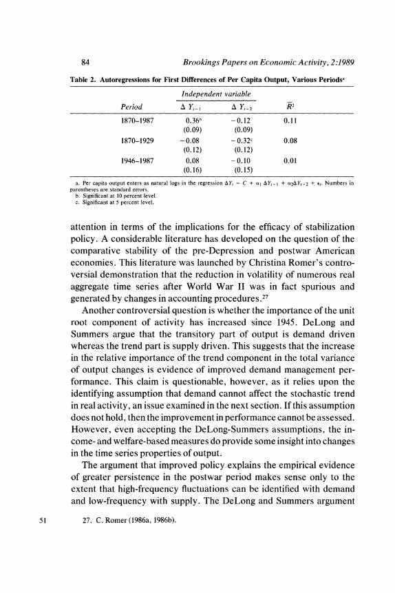
Table 2 reports second-order autoregressions for the output changes. The table reinforces the basic message of the spectral tests. None of the four autoregressive coefficients for the pre-Depression and postwar periods is significant at 5 percent and only one at 10 percent. The estimates over the entire sample reject a white noise specification because the AR(1) coefficient is significant. This finding is consistent with the rejection of white noise by the spectral tests. The reported standard errors are all asymptotic, so the significance levels should be interpreted with caution. But the qualitative message is clear-excluding the decline in the thirties and wartime recovery, output changes are only weakly correlated. More important, the point estimates of these first- difference autoregressions also imply that persistence is important for the entire sample and the postwar period. For the pre-Depression period, the Campbell-Mankiw measure is substantially less than one. For the postwar period, the Campbell-Mankiw measure approximately equals one. For the entire sample period, the measure exceeds one. As the formal hypothesis testing would suggest, figures 2 and 3 show spectral distributions much closer to the diagonal than that for the entire sample given in figure 1. The empirical results are consistent with the interpretation that the unit root component of annual GNP does in fact have economic significance. All three sample periods exhibit substantial persistence. For annual fluctuations, there is no unambiguous way of decomposing stochastic trends away from cycles.

The relative significance of the unit root component of output fluctuations in the pre-Depression and postwar periods has attracted much

26. Durlauf (1989d).


Table 2. Autoregressions for First Differences of Per Capita Output, Various Periodsa

Independent variable

Period A Y,, A Y,, R'

1870-1987 0.36b -0.12 0.11 (0.09) (0.09)

1870-1929 -0.08 - 0.32c 0.08 (0.12) (0.12)

1946-1987 0.08 - 0.10 0.01 (0.16) (0.15)

a. Per capita output enters as natural logs in the regression AY, = C + (x IY, I + t2AY,-2 + el. Numbers in parentheses are standard errors.

b. Significant at 10 percent level. c. Significant at 5 percent level.

attention in terms of the implications for the efficacy of stabilization policy. A considerable literature has developed on the question of the comparative stability of the pre-Depression and postwar American economies. This literature was launched by Christina Romer's controversial demonstration that the reduction in volatility of numerous real aggregate time series after World War II was in fact spurious and generated by changes in accounting procedures.27

Another controversial question is whether the importance of the unit root component of activity has increased since 1945. DeLong and Summers argue that the transitory part of output is demand driven whereas the trend part is supply driven. This suggests that the increase in the relative importance of the trend component in the total variance of output changes is evidence of improved demand management performance. This claim is questionable, however, as it relies upon the identifying assumption that demand cannot affect the stochastic trend in real activity, an issue examined in the next section. If this assumption does not hold, then the improvement in performance cannot be assessed. However, even accepting the DeLong-Summers assumptions, the income- and welfare-based measures do provide some insight into changes in the time series properties of output.

The argument that improved policy explains the empirical evidence of greater persistence in the postwar period makes sense only to the extent that high-frequency fluctuations can be identified with demand and low-frequency with supply. The DeLong and Summers argument

27. C. Romer (1986a, 1986b). 51


on the differences between pre-Depression and postwar business cycles relies on two parts. First, these authors require that the postwar series is relatively concentrated in the low frequencies. This means that

&9Ypre-Depression(X) - Ypostwar(X) f 0 X ? 0.

If this relationship does not hold for all X, then it is difficult to describe one of the two periods as dominated by a particular type of structural shock. Second, they claim that the postwar annual fluctuations are a random walk, whereas the pre-1946 period exhibits substantial mean reversion.

Figures 4 and 5 present the spectral distribution functions for the two periods, for both wealth and income fluctuations. The diagonal line represents the spectra'l distribution function for white noise that serves as a benchmark for the concentration of variance in high versus low frequencies. The estimates are computed through cumulation of the periodogram.

The spectral distribution functions indicate that the percentage of variance attributable to low-frequency movements is not strictly greater for the postwar period, for all possible definitions of "low" frequency. But there is an apparent tendency for the postwar period to exhibit more power at very low frequencies than does the pre-Depression. This feature is supportive of the qualitative claims of DeLong-Summers.

However, the goodness-of-fit tests in table 1 accepted the random walk null hypothesis for both periods. Similar results hold for the wealth series. Whatever role demand policy played, the view that the economy's performance has not improved is not rejected by the data.28 Therefore, the conclusion that postwar demand policy has somehow been superior in terms of consequences is not supported by the data. There is little basis for differentiating between the sources of pre-Depression and postwar fluctuations on the basis of the autocorrelation properties of output.

It is possible to argue that the macroeconomic policy in the postwar period has improved because we have avoided a recurrence of the Depression, but it is difficult to draw any statistical inference about a

28. A formal test based on the CVM statistic of the hypothesis that the pre-Depression and postwar spectral distribution functions are independent sample path realizations of the same stochastic process cannot be rejected at 5 percent.


Figure 4. Pre-Depression and Postwar Changes in Incomea Fraction of varianceb

1.0.... .

0.9

0.8 -

0.7-

0.6 - White noise Postwar .....

0.5 _-. /

0.4 ... I,

0.3 .. - < Pre-Depression

0.2

0 - 0 37r 7T

Hoo~ 4 2 4 (2) (8) (4) (2.67)

Frequency kc a. Income enters as natural logs. b. See figure 1, note b. c. See figure 1, note c.

change in the probability of an event that historically occurred only once in more than 100 years.

The results of this section may be summarized as follows. First, for annual data, it is difficult to reject the hypothesis that both the pre- Depression and postwar output series obey a random walk with drift. Other processes are certainly consistent with the data, but such processes will also exhibit substantial persistence. Second, wealth analogues to the output series fulfill the same quantitative conclusions as the output data in terms of the persistence. Third, there is little basis for discrimi- nating between the pre-Depression and postwar periods on the basis of the distribution of variance across frequencies. Specifically, the weight on the lower frequencies is not uniformly greater for the postwar period. Therefore, it is difficult to use the time series properties of pre-Depression and postwar output to reject Christina Romer's argument that there has been little improvement in the stability of the economy in the past 40 years. Any defense of the success of postwar stabilization policy will require that the structural sources of fluctuations be assessed.


Figure 5. Pre-Depression and Postwar Changes in Wealtha

Fraction of variance b

1.0

0.9 -

0.8 -

0.7 -White noise

0.6 -/

0.5 - Postwar ,.

0.4

0.3 - Pre-Depression

0.2 -

0.1~~~~~~~~~~~~~~0 0. I~~~~~~~~~~~ 0 t O 7c 7c I 7c (00) 4 2 4 (2)

(8) (4) (2.67) Frequency Xc

a. Wealth enters as natural logs. Discount rate equals 0.96. b. See figure 1, note b. c. See figure 1, note c.

Trends and the Structural Sources of Fluctuations

Many authors have interpreted the persistent components of economic activity as evidence that "real" factors play a primary role in fluctuations. The argument is roughly as follows. If the marginal product of capital diminishes to zero as the capital-labor ratio becomes unbounded, then a given technological configuration implies a bounded production set for the economy. Unit roots in output imply that the production set is asymptotically unbounded. Random and persistent shocks to the production possibility frontier can be explained only as technical change. This perspective has been widely adopted in empirical work. The interpretation of long-run movements of GNP as generated by "real" factors has been treated as an identifying assumption in supply-demand decompositions by Blanchard and Quah and by Matthew Shapiro and Mark Watson, among others.29

29. Shapiro and Watson (1988).


This argument has the powerful policy implication that demand factors are unimportant in improving social welfare. Recent research has suggested that the stochastic growth element of output is the major deter- minant of lifetime individual welfare. This result was demonstrated by Robert Lucas when he calculated that elimination of the volatility of output would improve social welfare less than would a small increase in the economic growth rate.30 Stabilization policy has little effect on long- run growth rates in the representative agent-real business cycle world. Fiscal policy plays a potentially important role in affecting the marginal return on capital. Demand management through anticipated monetary and fiscal policy is generally neutral.

DeLong and Summers have argued that the Lucas claim that fluctuations are irrelevant is flawed by the assumption that the mean of output over the cycle cannot be affected by government policy. They argue that the gap between potential and actual GNP is always nonnegative. Successful stabilization policy will close these gaps. Their argument does not go far enough in that it accepts the trend-cycle dichotomy for policy efficacy. This section presents some empirical evidence that suggests that the trend component of activity cannot be presumed to evolve independently of domestic institutions and policies. The next section of the paper takes up the question of persistence and macroeconomic theory.

International Aspects of Persistence

The interpretation of unit roots as being due to technology is difficult to reconcile with the substantial differences in output dynamics across advanced industrialized countries.31 If technological shocks represent the basis of persistence in output innovations, then one would expect that the long-run growth rates of industrialized countries would be related at least with lags. One test of the technology interpretation of persistence is the tendency of permanent innovations in one country to migrate eventually to another. Some evidence against this proposition has already been documented by Campbell and Mankiw in their analysis

30. Lucas (1987). 31. Stockman (1988) performs an analysis related to what follows by performing a

variance decomposition of sectoral output fluctuations across several countries. Stock- man's results parallel the long-run results presented below.


of unit root components in seven OECD countries.32 They observe that there is little relationship at a national level for quarterly unit root components of output. This section extends their evidence in two directions using annual data on log per capita output for six major industrial economies.

A first set of tests explores the long-run dynamics relating permanent innovations in international output.33 Under a productivity interpretation of permanent innovations, technology advances in one country should be associated with technology advances in another. If there is a permanent shift in the production possibilities per capita in one country, there should be an eventual movement in other countries. From the time series perspective, output in advanced countries should be cointegrated. Cointegration means that two time series possess a common persistent component, so that some linear combination of the series should be free of any persistent component. In the context of interpreting output persistence, for countries i andj, the null hypothesis of interest is: there does not exist a y such that GDPi - yGDPj is a stationary process. When the null hypothesis holds, a permanent shock to long-run GDP in one country fails to be associated with a permanent change in the other country. Under the null, there is no tendency for permanent innovations in one economy to be manifested in another. This means that the stochastic growth rates of countries can diverge. It is difficult to understand how this divergence may occur if permanent shocks to output growth are purely technology based, as this would mean that technical change never migrates across countries. Notice that these tests of cointegration place relatively weak restrictions on technology movements because they do not require that permanent shocks fully transfer from one country to another.

The cointegration tests were originally derived by Engle and Gran- ger.34 These authors observed that if two integrated time series are not cointegrated, then the residuals Ei, in the regression,

(14) GDPi, = C + yGDPj,, + Eij,

32. Campbell and Mankiw (1989). 33. The international comparisons use gross domestic product rather than gross

national product because of data availability. 34. Engle and Granger (1987).


will contain a unit root. A second-stage regression on the residuals from equation 14,

(15) Ei :-PlEi,-l + P2,AEi,t_j + uij,,

will produce a coefficient Pi equal to zero, since an explosive process such as EI, can never explain a stationary process such as AEij. Under the alternative, where Eij is stationary, this will not occur. The null hypothesis may therefore be tested by computing the t-statistic for Pi in this regression.

Table 3 reports the results of bivariate cointegration tests for the log of per capita output between Japan, West Germany, France, the United Kingdom, Canada, and the United States.35 The null hypothesis in the tests is that the time series are not cointegrated, that is, that E,i is nonstationary. As the table indicates, in all of 15 possible cases the null hypothesis is accepted. Some degree of close long-term links between the U.K. and Canadian and the U.S. and Canadian economies is reflected in cointegration at the 10 percent level of significance. It would be difficult to attribute these links to a unique similarity in national production functions. The collective results of this table strongly suggest the importance of domestic conditions and institutions in determining the long-run characteristics of economic growth.

The cointegration tests may be reinforced by a direct consideration of the properties of the differences of log per capita output in the various countries. The idea that growth rates across different countries converge can be expressed through an examination of the time series properties of GDPi, - GDPj,t. If the autoregressive representation of this difference contains a unit root-that is, the autoregressive coefficients sum to one- then there is no tendency for the per capita output levels in the two countries i andj to converge.

Table 4 presents the second-order autoregressions for all bivariate log per capita output differences. In 12 of the 15 cases, the autoregressive coefficients sum to a value of at least 0.95. For 8 of the 15 cases, the

35. All data are log per capita real gross domestic product, 1950-85. The series used are reported in Summers and Heston (1988). These data are widely regarded as the best available series for cross-country comparisons of real activity because of the care with which exchange rate and price information are incorporated into the construction of the aggregate real series from nominal observations.


Table 3. Cross-Country Cointegration Tests, Per Capita Output, 1950-85a

West United United Country France Germany Kingdom Canada States

Japan - 1.79 - 2.59 - 1.35 - 1.90 - 2.28 France - 2.53 - 0.93 - 1.89 - 2.28 West Germany - 1.86 - 2.16 - 2.55 United Kingdom - 2.96b -3.00b Canada - 2.20

a. Values reported are t-statistics of the coefficient pi in second-stage regression AEi, = pi E,ij I + P2 AEi,t i +

ujt, which follows from the regression GDPj,, = C + yGDPj,t + eij. Per capita output enters as natural logs of real GDP.

b. Significant at 10 percent level. No results are significant at 5 percent level.

coefficients sum to at least 0.98. Further, the point estimates are generally not significantly different from one.36 These results mean that there is little evidence of convergence. The point estimates further demonstrate that the acceptance of the no-cointegration null in table 3 cannot be dismissed as stemming from lack of power in the tests. Over the postwar period, permanent innovations to output in one country do not appear to have necessarily affected other countries.

The lack of close interdependence is confirmed when one considers the relationship between output changes in the six countries of interest. This analysis is sensitive to short-term links between economies. John Geweke has developed a very general framework for understanding the linear interactions of multiple time series.37 The basic idea is to start with the univariate autoregression of country i's output changes,

(16) AGDPi,t = 3 + a(L)AGDPj't_ + Eist,

and ask how knowledge of the behavior of output changes in another country improves the univariate forecasts. If the lagged output changes for another country are included,

(17) lAGDPi, = 3 + rT(L)AGDP ,t_l + y0(L)AGDPj,t_l + qj,tq

36. Formal testing employing Dickey-Fuller regressions with Phillips-Perron corrections employing a Bartlett window of length 10 found that for regressions including time trends, the null of a unit root was accepted for all 15 pairs. When the time trend was omitted, the null was accepted for 12 pairs, the exceptions being West Germany-United Kingdom, West Germany-Canada, and West Germany-United States.

37. Geweke (1982).


Table 4. Autoregressions of Cross-Country Differences in Per Capita Output, 1950-85a

Independent variable

Cross-country Cross-country Sum of Country i Country j difference, difference, 2 coefficients

Japan France 1.62 - 0.62 1.00 (0.14) (0.13)

West Germany 1.60 -0.61 0.99 (0.14) (0.13)

United Kingdom 1.79 -0.79 1.00 (0. 1 1) (0. 10)

Canada 1.58 - 0.59 0.99 (0.14) (0.14)

United States 1.68 -0.69 0.99 (0.13) (0.12)

France West Germany 1.47 -0.56 0.91 (0.15) (0.13)

United Kingdom 1.31 -0.32 0.99 (0.17) (0.16)

Canada 1.08 -0.11 0.97 (0.17) (0.16)

United States 1.26 -0.28 0.98 (0.17) (0.16)

West Germany United Kingdom 1.47 -0.49 0.98 (0.16) (0.15)

Canada 1.48 - 0.52 0.96 (0.16) (0.14)

United States 1.58 -0.61 0.97 (0.15) (0.13)

United Kingdom Canada 0.85 -0.03 0.82 (0.17) (0.17)

United States 0.81 0.02 0.83 (0.16) (0.16)

Canada United States 1.05 -0.10 0.95 (0.16) (0.16)

a. Per capita output enters as the natural log of real GDP in the regression GDPj,, - GDPj, = C + a1 (GDPi,t_, - GDPj,t,_) + aQ (GDPi,t-2 - GDPj,t-2) + Ei,j,. Numbers in parentheses are standard errors.

then a test of the null hypothesis that yo(L) = 0 is a Granger causality test. Contemporaneous interactions may be captured through

(18) AGDPi,t= 3 + ar(L)AGDPj,t_j + y0(L)AGDPj,t_l + y,AGDPj, + Ci,t*


Finally, one can ask how future changes in output in one country help predict qhanges in another:

(19) AGDPi,, = 3 + r(L)AGDPi,, - + yO(L)AGDPj, -I + YIAGDP1,t + Y2(L-I)AGDPj,t+1 + vi,.

Collectively, these different regressions give a comprehensive picture of the linear interactions between two series of output changes. The greater the interactions between two economies, the greater the improvement in forecasting ability one output series helps provide for another. Geweke proposes three measures of feedback:

(20) FAGDPj, AGDPi log - -'

FAGDP. A AGDP1 log-%2

FAGDPj AGDPi log -i

These statistics, roughly speaking, measure the percentage improvement in reducing the forecast error of one variable by employing different combinations of another. The first statistic measures the total predictive power one series adds to another; the second statistic measures causal predictive power; the third statistic measures contemporaneous predictive power. If Y0, ,Y, Y2 are all equal to zero, this means that there are no linear interactions between the series either contemporaneously or with leads and lags. When this condition holds, it means that there is a structural representation of the two time series:

(21) AGDPi,t = Ci + i(L) Ei,t,

AGDPj,t = Cj + ej(L) Ej,,,

where Ei,t and Ej,t are white noise innovations uncorrelated with each other at all leads and lags. From the perspective of linear interactions, the time series are independent.

Table 5 reports the estimates of the bivariate feedback across changes in output for six of the major industrial economies. Fairly weak evidence of feedback exists between the different combinations of countries. The first column reports the tests of the Geweke total feedback measure between the different pairs of countries. Every test statistic is insignifi-


Table 5. Geweke Feedback Statistics for Cross-Country Fluctuations, in Per Capita Output, 1950-85a

Measlures offeedback between countries

Causal feedbackc Contempor- Total aneous Country i Country j feedbackb j to i i to j feedbackd

Japan France 0.20 0.01 0.05 0.14e West Germany 0.10 0.01 0.00 0.09 United Kingdom 0.11 0.05 0.01 0.05 Canada 0.04 0.00 0.03 0.01 United States 0.04 0.00 0.00 0.04

France West Germany 0.22 0.00 0.02 0.201 United Kingdom 0.13 0.01 0.00 0.12e Canada 0.08 0.00 0.03 0.05 United States 0.06 0.01 0.00 0.05

West Germany United Kingdom 0.14 0.01 0.00 0.13e Canada 0.12 0.07 0.00 0.05 United States 0.13 0.01 0.01 0. le

United Kingdom Canada 0.03 0.00 0.01 0.02 United States 0.10 0.00 0.00 0.10

Canada United States 0.471 0.01 0.01 0.451

a. Feedback statistics (defined below) use results from the following system of regressions: AGDPj,t = p + 7r(L)AGDPj,t_t + Eilt,

AGDPi,t = p + 7r(L)AGDPi,t,_ + -o(L)AGDPj,t,_ + Th,t,

AGDPi,t = p + 7r(L)AGDPi,t,_ + -o(L)AGDPj,t,_ + -y AGDPj,t + kj,t, AGDPi,t = p + r(L)AGDPi,t1_ + -o(L)AGDPj,t_j + -y AGDPj,I + Y2(L- )AGDPj,t+1 + vi,,. Per capita output enters as first differences in the natural log of real GDP. Significance levels based on F-statistics. All lags and lead polynomials of order two.

b. Total feedback equals log ((I2/(2). The null hypothesis is that yo, yj and Y2 equal zero. c. Causal feedbackj to i equals log ((oI2/U). The null hypothesis is that yo equals zero. d. Contemporaneous feedback equals log (f2/(I2I). The null hypothesis is that -y equals zero.

e. Significant at the 10 percent level. f. Significant at the 5 percent level.

cant except for the United States and Canada. The second and third columns report the Granger-Sims causality tests for all country pairs. For none of the country pairs is there any evidence of causal feedback between output fluctuations. The fourth column indicates that there is little contemporaneous correlation in innovations. Even though the contemporaneous feedback values are larger than the causality feedback numbers, only France and West Germany and the United States and Canada show a statistically significant relationship. These isolated relations are more easily interpreted as signs of market integration than uniquely similar production functions.

The results of tables 3, 4, and 5 in total suggest that innovations in real activity do not exhibit strong linear transmission mechanisms. A


salient characteristic of the postwar period is the lack of identifiable dependence of aggregate fluctuations across economies.38

One answer to these test results is that the source of the supply fluctuations is idiosyncratic at a domestic level and not transferred through imitation. As an example, if all technical innovations were successfully protected by patents, then a supply-side explanation of unit roots would appear to be consistent even though output is not cointegrated across countries. However, this sort of explanation can still be linked to demand-side factors through the issues of investment incentives. Investment rates would control the diffusion of new technologies, albeit with some lag structure. The results of tables 3 and 4 find no feedback even with long lags. The sorts of models that render the growth rates across countries autonomous in turn require some sort of aggregate complementarity in production in the presence of incomplete markets, as in Paul Romer's model of social increasing returns to scale. In this case, the social return to capital accumulation is greater than the private return. In such a world, there will be no necessary long-run coherence in growth rates across economies. However, this is precisely a circum- stance of the dynamic coordination failure that is discussed below. In models of dynamic coordination failure, demand-side fluctuations can interact with the evolution of technology to determine a growth rate.

Intersectoral Aspects of Persistence

A second test of the technology interpretation of unit roots involves a comparison of growth innovations in the major sectors of the American economy. If aggregate unit roots are generated by technology, it is unlikely that growth innovations will be common across sectors. Tech- nical change in agriculture does not imply technical change for finance, insurance, and real estate. There is, however, considerable evidence of coherence across sectors within the American economy.

Preliminary to exploring the coherence of the long-run properties of the American industrial sectors, unit root tests were performed on 13

38. One does not want to push these results too strongly. Clearly the slump across Europe in the 1980s was not generated by coincidental output declines. The point is that there is no statistical evidence of a systematic relationship between contemporary fluctuations over the past 30 years.


Table 6. Unit Root Tests of Sectoral Per Capita Output, 1947-87a

Sector i t-statistic

Agriculture -2.01 Mining - 1.02 Construction - 3.20 Durable manufacturing - 3.90b Nondurable manufacturing - 2.10 Transportation - 2.80 Communication - 1.20 Electricity, gas -2.40 Wholesale trade - 1.80 Retail trade - 3.54c Finance, insurance, real estate - 0.14 Services - 3.20 Government - 2.50

a. Numbers are t-statistics with Phillips-Perron corrections of y in the regression GDP,t = C + Pt + yGDPi,,_ I + E,t. Per capita output enters as the log of real GDP.

b. Durable manufacturing was the only sector significant at the 5 percent level. All other sectors rejected the null hypothesis that y equals one, thus supporting the theory that there is a unit root in sectoral GDP.

c. Significant at 10 percent level.

different components of the national income and product accounts.39 A separate time trend was included in each regression to control for changing sectoral weights. With GDPi,, denoting the log of per capita output in sector i, the regressions took the form

(22) GDPi,, = C + Pt + yGDPi,,t + Ei,t.

The null hypothesis is y = 1. The t-statistics for the null, modified by the Phillips-Perron correction, are reported in table 6.40 For 12 of the 13 sectors, the hypothesis of a unit root is clearly accepted. The one exception is durable manufacturing. The t-statistic is marginally significant at 5 percent. Evidence below, however, accepted the null hypothesis that the log per capita durables series is a random walk with drift. It is therefore reasonable to conclude from these various tests that the sectoral series all exhibit substantial persistence.

Table 7 reports the dynamics of output changes in the various sectors

39. All sector level data was taken from Citibase. The data are log per capita annual output. The data in levels sum to gross domestic product. The data run from 1947 to 1987.

40. These tests are based upon the Phillips and Phillips-Perron generalizations of the Dickey-Fuller tests for unit roots. All Phillips-Perron corrections employed Bartlett windows of length 10. See Phillips (1987) and Phillips and Perron (1988) for the asymptotic theory and Fuller (1976) and Dickey and Fuller (1981) for significance levels of the test statistics.


Table 7. Sectoral Per Capita Output Equations, 1947-87a

Independent variable CVM

Sector i AGDPi,,- I AGDP,, 2 statistic

Agriculture -0.21 - 0.31 0.19 (0.15) (0.15)

Mining 0.03 -0.14 0.04 (0.15) (0.16)

Construction 0.53b 0.07 0.65b (0.15) (0.14)

Durable manufacturing - 0.04 -0.15 0.05 (0.16) (0.16)

Nondurable manufacturing - 0.09 - 0.34c 0.15 (0.15) (0.15)

Transportation 0.18 -0.28c 0.18 (0.14) (0.14)

Communication - 0.03 0.22 0.06 (0.15) (0.14)

Electricity, gas 0.20 0.30 0.56b (0.15) (0.55)

Wholesale trade 0.04 -0.21 0.06 (0.15) (0.15)

Retail trade 0.01 -0.18 0.06 (0.16) (0.16)

Finance, insurance, real estate 0.30c 0.26 0.93b (0.15) (0.15)

Services 0.26 - 0.06 0.29 (0.15) (0.15)

Government 0.37c -0.07 0.48c (0.16) (0.15)

a. Per capita output enters as first differences in the natural log of real GDP in the regression AGDP,t = C + a, AGDPi,,-I + a2 AGDPO,,-2 + (i,. Numbers in parentheses are standard errors.

b. Significant at the 5 percent level. c. Significant at the 10 percent level.

along with the CVM statistics. For the AR(2) specification, only construction exhibited a statistically significant (at 5 percent) coefficient. As the third column indicates, 10 of the 13 sectors exhibited CVM statistics consistent with the random walk null. The aggregate dynamics are largely mirrored on the sectoral level, reinforcing the significance of persistence by illustrating that it is not an artifact of aggregation. It also indicates the existence of some deviations in long-term behavior across components of the economy, rather than complete symmetry across sectors.


Tables 8 and 9 explore the interactions of the sectoral growth with one another through two methods. The first technique considered the cointegration of individual sectors with measures of aggregate activity. The basic idea was to exploit the fact that cointegration is a transitive property; two series, each cointegrated with aggregate output, will themselves be cointegrated. Again letting GDPi,t denote log output in sector i at time t, and GDP, denote total log gross domestic product at t, if GDP, - yiGDPi,t and GDP, - yjGDPj,t are stationary processes, then yiGDPi,t - yjGDPj, must be stationary as well, which means the sectors are cointegrated. Table 8 reports tests of the cointegration of the 13 NIPA sectors with gross domestic product and total private industrial production. The table indicates that the great majority of sectors are cointegrated with both aggregates and by extension with each other. The noteworthy exception to this finding is the failure of durable manufacturing to be cointegrated with either aggregate. This failure proved to be robust to different specifications of the cointegrating tests. Table 9 reports bivariate cointegration tests across the different sectors and demonstrates that there is substantial but by no means universal cointegration across sectors. Agriculture, mining, and construction do not exhibit much cointegration with the other sectors. The transitivity of cointegration makes these results somewhat inconsistent with the previous table, which would have predicted a greater degree of cointegration across sectors. The economywide aggregates apparently smooth out some idiosyncratic components to sectoral fluctuations. The appropriate conclusion seems to be that there is substantial but not complete cointegration at a sectoral level.

Three features of sectoral output behavior stand out. First, unit roots and random walk behavior exist at the sectoral level and mimic the aggregate output series. Second, a substantial degree of cointegration exists between sectors. This is difficult to reconcile with the technology interpretation of unit roots if the shocks to technology across sectors exhibit some independence. Third, not all sectors are cointegrated, meaning that some divergence in growth patterns does occur.

These results make it difficult to interpret stochastic trends in real activity as the outcome of exogenously evolving random technology shocks, unless one assumes that the dimensionality of productivity shocks is substantially smaller than the number of sectors. This is especially difficult to believe, when one observes the cointegration of


Table 8. Sectoral Cointegration Tests between Aggregate and Sectoral Per Capita Output, 1947-87a

Aggregate output

Sector i GDP pjpb

Agriculture - 3.30c - 3.30d Mining -4.20c - 4.00c Construction -2.50 - 2.80d Durable manufacturing - 1.70 - 1.10 Nondurable manufacturing -4.50c - 3.70c Transportation - 2.80d - 2.30 Communication - 3.50c - 3.00d Electricity, gas - 3.60c - 3.80c Wholesale trade -3.20c - 2.80d Retail trade -3.00d - 2.30 Finance, insurance, real estate - 3.20c - 3.60c Services - 2.70 - 2.50 Government 4.20c - 4. 10c

a. Numbers are t-statistics for pi in the second-stage regression of AEi,t = Pl Eijt I + P2 AEi,t + ui,,. This follows from the regression of sector output on C + yX, + Ej,. The variable Xt equals, first, GDPt and then PIPt. The null hypotheses is that pi equals zero. Significance levels are taken from Engle-Granger (1987).

b. Total private industrial production. c. Significant at the 5 percent level. d. Significant at the 10 percent level.

technologically disparate sectors such as mining and nondurable manufacturing. Hence, it seems important to consider alternative explanations of how sectors within one economy are linked over the long run.

Coordination Failure and Unit Roots

The supply or productivity interpretation of unit roots rests in part on older macroeconomic theories in which demand shocks could only be transitory, and ignores much of the current thinking on the microeconomic foundations of macroeconomics. The view that demand-side shocks are temporary evolved from the traditional assumption that deviations from the neoclassical equilibrium occur because prices exhibit short-run stickiness. This stickiness disappears over time in response to market pressures. Demand innovations generate real effects only to the extent they affect the wedge between equilibrium and current prices. From such a perspective, demand shocks naturally generate transitory effects when they fail to affect the production set that defines economic

0 - en000

0 00000 0 0

(X~I I r m II _ c s +

EII II I I1I11 I11 I1

_ cs e cs _ t _ ̂ a

I I I II I I I I I I 0

5S o 00 0 008 n00 t - .0 -e: \ C rNoW o }obNo

CZ .r . .C

00~~~~~~~~~~

0~~~~~~~~~~~~~~~~~~0

ob 0 -o- bi 0

I I I I I I I

.W

rs 000, 0 0 0 00 g

? 5; O 0 - 0 o0 0 _

0 I

_ S: or-o go a.E

Cu~ ~ ~~~~~~~~C C Co

.o 0e I I I I I

- 0~~~~~~~~~~~~~cr Z 0~

Cu 0 Q :n= MQQ E

CU 0)? S U: F U w 3 42


activity. The dynamic structure of these models equates the long run with the neoclassical equilibrium. Recent economic theory, however, has emphasized the role of incomplete markets, imperfect competition, and other imperfections in generating multiple equilibriums and coordination failures. This view of the limitations of the Arrow-Debreu paradigm in turn leads to long-run feedback from demand shocks to aggregate activity.

Much of the new theoretical macroeconomics centers on the difficulties of coordinating activities in modern economies. The basic idea behind this class of models is straightforward. In a world of incomplete markets, there can exist externalities to market activity by individual industries or firms. For example, Peter Diamond has developed a model in which, if trading partners are difficult to find, then the act of producing and engaging in search will increase the probability of executing successful trades for all potential producers. Walter P. Heller has demonstrated how imperfect competition can induce multiple intersections of the marginal cost and marginal revenue schedules. When a firm increases output, it raises demand for all sectors in the economy. Similarly, Kevin Murphy, Andrei Shleifer, and Robert Vishny have presented models in which high levels of production induce sufficient demand to justify the payment of fixed costs necessary for the employment of efficient technologies. And John Bryant, Paul Romer, and Robert Lucas have shown that external or social increasing returns to scale at an economywide or industrywide level lead to production complementarities or social increasing returns to scale that cannot be captured by an individual firm. All these approaches raise the possibility of multiple steady-state levels to economic activity. These different approaches generally fall under the rubric of "thin market externalities." The hallmark of this class of theories is the compatibility of different levels of real activity with the same microeconomic specification of individual firms and consumers. The key source of the multiplicity of long-run equilibriums is the positive effect that high production by some set of agents has on the decision of others to produce. Paul Milgrom and John Roberts have named this property "positive complementarities. " 41

41. Diamond (1982); Murphy, Shleifer, and Vishny (1988); Heller(1986); Bryant (1983); P. Romer (1986); Lucas (1988); Milgrom and Roberts (1988). Cooper and John (1988) provide a valuable unifying framework for many of these models.


When one considers how multiple equilibriums interact with technical change, then it is possible to show that coordination failures can induce unit roots in realized activity. Suppose that technical change is deterministic at the level of invention in the sense that the rate of invention is constant over time. Each invention, if fully implemented, is equally valued and will add y to the aggregate output of society. In this case, long-run output Y, fulfills

(23) Y, = yt.

Realized economic growth will be deterministic only to the extent that each new technology leads to the same economywide implementation. If there are multiple equilibriums for the implementation of each technology, and these equilibriums endogenously evolve in response to various random events, then the realized activity associated with invention i will equal a random variable (i. Aggregate activity will represent a sum of random variables:

(24) Y, = E (i j=0

This income process contains an exact unit root. As I have shown elsewhere, unit roots induced by coordination failure do not require specialized parameter assumptions or specialized production functions.42 Sims's argument on the theoretical improbability of unit roots applies only to representative agent models. In dynamic coordination problems, unit roots are the natural outcome of many agents sequentially acting through decentralized markets.43

A simple model illustrates the basic way in which aggregate activity may be compatible with different equilibriums based on different realizations of productivity shocks." The idea of the model is to demonstrate

42. Durlauf (1989a, 1989b). 43. For a different perspective on the endogenous evolution of unit roots in aggregate

output, emphasizing the uncertainty associated with invention, see Aghion and Howitt (1989).

44. This example differs from the standard models of coordination failure in that it possesses a mechanism for the endogenous evolution of an economy toward one of several possible equilibriums. This feature differs from most papers in the literature that prove the existence of multiple steady states without explaining how a particular state arises. See Durlauf (1989a) for further development of the idea that equilibriums are endogenously determined as realizations of complex stochastic processes. Specifically, the paper shows how initial conditions and expectations for the future behavior of the economy interact to affect the selection of a particular equilibrium.


how isolated complementarities in economic behavior can generate rich aggregate dynamics. Consider an infinite number of industries equally spaced along a line.45 Each industry has access to a separate labor pool and the wage rate is normalized to equal one. Each industry has access to two modes of production. One mode is subject to a productivity shock (i ,. The technology is nonconvex in two senses. First, one technique is subject to a fixed cost K. Second, the technologies are jointly nonconvex as labor must be employed in only one of the two technologies.46 The production in industry i, Yi,t, follows

(25) Yit = f1(Li,, (i,t) - K,

if technique one is chosen, or

(26) Yit = MLi,),

if technique two is chosen. By assumption, f1'() > f2'(). The assumption that firms face fixed costs to high-scale production is

standard in the coordination literature. Several justifications exist for supposing that industries face nonconvex production decisions of this sort. One source of the fixed cost, according to Diamond, is transactions costs. Output levels above a certain threshold may require economywide search to enter new markets and find customers. A second source is embedded in the Akerlof-Yellen fair wage models.47 In these models, worker morale and productivity are determined by whether or not workers perceive their employment conditions as fair. Higher productivity among workers can be induced by higher wages. The fixed cost K may be treated as overhead capital necessary to utilize workers in highly productive activities justifying the high wages.

Alternatively, the nonconvexity of the production set can be a direct result of fixed costs to the organization of complicated production processes. Milgrom and Roberts have developed a view of manufacturing activity that emphasizes the nonconvexities associated with a firm simultaneously choosing inventory policies, marketing strategies, and

45. Each industry consists of a large set of identical firms. Each firm faces a production decision that consists of choosing a mode of production as well as a level of production. Since firms are identical, the industry decision will be identical to the firm decision. The distinction between firms and industries is made exclusively to justify a Nash equilibrium concept for the interactions of industries.

46. The idea of modeling technological nonconvexities as firms as facing different choices of technique was introduced into the coordination literature in Cooper (1987).

47. Akerlof and Yellen (1988, 1989).


production techniques.48 The impact of each of these variables on the payoffs associated with the others renders the production set nonconvex. One approximation of this nonconvexity is a fixed cost.

The links within and across industries over time will be determined by the behavior of the productivity shocks i,. Specifically, (i, is assumed to depend only on the production techniques chosen by industries i and i - 1 in the previous period. If Prob() denotes a probability density and Q.- I denotes the state of the entire economy at t - 1,

(27) Prob(ti,,|I Q,t-1) = Prob(ti,| (xi- I,- I xij .1),

where xi, = I if technique one is chosen at t by industry i and xi, = 0 if technique two is chosen at t by industry i.

The basic idea is that high-efficiency, low-marginal-cost production in one industry spills over to affect production positively in another industry. Onejustification for this interaction is that there exists a social increasing-returns-to-scale production function. This is the argument initiated by Arrow and generalized by Paul Romer.49 For example, innovations in one industry may suggest efficiencies in other industries through imitation. High levels of activity in contiguous industries may reduce consumer search costs and producer advertising costs and thereby increase total product demand.

A second justification may be sociological. Following Akerlof and Yellen, suppose that worker attitudes concerning fairness fall into one of two categories. Workers who fall into category two require a larger wage premium than workers in category one to induce high productivity. Further, suppose profit-maximizing firms require category one workers to justify high production levels. If attitudes among workers in a given labor market are a random variable that is a function of the attitudes and behavior of other worker groups, then one will observe complementarities across labor markets. The links in the productivity shocks could be links defining worker attitudes.

A third source for this interdependence may be market structure. Suppose firms follow constant-markup pricing policies

(28) Pi,= =J '(Li,),

if technique one is chosen, and

48. Milgrom and Roberts (1989). 49. Arrow (1962).


(29) PO, = [1f2 (Li,),

otherwise. If industry i - 1 produces some type of overhead capital that augments the marginal productivity of labor in industry i, then the same sorts of spillovers will occur.

Firms maximize output in each period. Labor is allocated to the first technique if the greater productivity of the technique justifies payment of the fixed production cost. In equilibrium, each industry makes a choice of technique based on the level of productivity induced by the state of the economy last period.50 From the perspective of dynamics, the essential equilibrium relation is the conditional probability charac- terizing industry i at t, wit, based on the history of the economy Q,_ 1. From the model's assumptions, the conditional probability that an industry produces at the high production level at t based upon the state of the economy at t - 1 fulfills

(30) Prob(i,t I | f1) = Prob(wi,t | x-1,t-1, (i,,-1).

Since each industry is thought of as a collection of small firms, industries cannot coordinate their behavior to capture the various complementarities. There do not exist economywide markets in which industries can coordinate intertemporal production plans to achieve an efficient equilibrium. Such markets are ruled out by assumption due to transactions costs and moral hazard problems. Each industry makes a choice of technique based upon the history of the economy and without consideration of the effects of the choices on future productivity.

This model will generate very interesting dynamics, depending on the structure of the conditional probabilities of high-level production. To relate the complementarities discussed so far to these probabilities, assume first that

(31) Prob(wi, = 1I-1,h1 = it- i 1l) -1.

50. To place the model in a general equilibrium framework, one needs to add a representative consumer who maximizes

EOU = lim I 'k- I' E [U(C ,) + (L - Li,)], k-#- I=O i=O

where Ci denotes consumption of good i, subject to a budget constraint that accounts for all wages and profits in the economy. The equilibrium prices determine the level of consumption demand, which in turn determines the level of labor employed in each industry. See Durlauf (1989b) for details.


All industries producing at a high level thus will constitute a stationary equilibrium. High levels of production across different sectors are mutually reinforcing. On the other hand, if some industries are not at a high production level, that will affect the productivity of the economy in the next period and mean that there is a positive probability that some industries choose low production levels. This idea is formalized through choosing a set of probability weights Oi < 1 such that

Prob(i, = I |i -1t-I = 0, (Ii,t-I = 1) =

(32) Prob(wi,t = Wi- 1,t-1 = 1 (A)i,t-I = 0) = 02,

Prob(oxi,= = I = ?, Wi,t- I = 0) = 03.

The critical question in terms of the economy's long-run behavior is whether for an arbitrary set of initial conditions, economic activity converges to the high-level steady state. If not, then there are multiple steady states in the economy. The existence of multiple long-run equilibriums turns out to depend critically on the 0 parameters.5' If 01, 02, 03 are all greater than 0.5, then for any initial configuration the economy will converge to all high-efficiency production. If 01, 02, 03 are all less than 0.5, then one can show that the system will never converge to the high-efficiency equilibrium if all industries start at the low-efficiency level. For different initial conditions, the economy endogenously evolves to different long-run levels of activity. The low-efficiency levels of different sectors are thus also mutually reinforcing.

A dynamic coordination problem of this sort can generate rich aggregate dynamics. To see this, an 80-industry version of the economy was simulated for different parameter values, starting from initial conditions of all low-production industries. In the exercise, industry production functions were chosen so that technique one always produces one unit of output and technique two produces zero units. For the parameters 01 = 0.15, 02 = 0.10, and 03 = 0.05, average output Y, converges to a process with mean 0.06 and autoregressive representation

(33) Y, = 0.04 + 0.25 Y,_ + 0.06Y,_2.

51. The multiple equilibriums in this model are formally analyzed in Durlauf (1989b). The underlying mathematical theory demonstrating the existence and possible nonunique- ness of an equilibrium may be found in Stavskaya and Pyatetskii-Shapiro (1968) and Vasilyev (1970).


For the parameters 01 = 0.3, 02 = 0.25, and 03 = 0.2, average output Y, converges to a process with mean 0.39 and autoregressive representation

(34) y, = 0.09 + 0.67Y,_1 + 0.07 Y-2-

As the values of the probability parameters increase, substantial autocorrelation emerges. It is also possible to show that there is substantial cross-industry correlation. Contiguous industries, defined in terms of the intertemporal probability links defining output choices, will tend to move together.

If new technologies require many industries to coordinate activities, then the multiple equilibriums of this model can occur for a fixed sequence of innovations. In particular, if each innovation creates a new set of industrial links along the lines described, then multiple equilibriums will exist for long-term growth. The generalization of multiple equilibriums to technical change is straightforward once one treats technical change as the interactions of a set of economic activities rather than the vibrations of a single production function. Elsewhere I have shown how coordination failures can interact with a deterministic linear technology trend to produce a random walk with drift in aggregate activity.52 If technical change represents the development of a new set of interrelated production opportunities, then the effect of these opportunities on actual output depends on the resolution of numerous coordination problems. Each invention therefore has a stochastic effect on activity.

The government will play a potentially significant role in the long-run behavior of output in the model. Since the economy will converge to a high-activity equilibrium for large enough values of the O's, it is clear that tax incentives and production subsidies will play a critical role in the determination of the long-run mean of activity. By adding capital to the model, investment tax credits become extremely important.

One can also envision a role for monetary policy. Suppose industries must borrow for capital investment to shift from low to high efficiency. If credit rationing occurs, then the probabiity of successfully borrowing to purchase capital will affect the O's in the model. Credit rationing models as developed by Alan Blinder and Joseph Stiglitz or Bruce Greenwald and Stiglitz suggest that Federal Reserve policies can have

52. Durlauf (1989a).


long-run consequences by increasing the probabilities of loans occurring when desired.53

Finally, it is straightforward to modify the model to incorporate demand-side effects. If efficient production requires a minimum scale, then individual industries will require high market demand in order to produce with technique one. The complementarities in the model can be constructed as demand driven in the sense that high levels of production in one industry lead to high demand in another. This idea underlies the work of Heller and of Murphy, Shleifer, and Vishny.

Stabilization policy in coordination models is equivalent to the cre- ation of production incentives that cause individual agents to internalize the social effects of their production decisions. Successful policy will affect the mean as well as the variance of output-gaps as well as cycles, to use DeLong and Summer's terms. However (to extend their perspective), successful stabilization policy will affect the stochastic trend as well as the cycle.

Historical and microeconomic analyses of technical change typically represent innovations as a set of new interacting production opportunities arising for an economy rather than a monotonic shift in a single production function. From these perspectives, dynamic coordination problems are an essential feature of economic growth. Much of the Stanford tradition in economic history, exemplified by the work of Paul David and Nathan Rosenberg, has interpreted the evolution of technology in this way. In his famous example of QWERTY, the organization of keyboard letters, David has shown how the typewriter evolved as an element of "a larger, rather complex system of production that was technically interrelated."54 Typewriter operators, producers of typed products, all interacted in a decentralized, sequential manner to imple- ment innovations in typesetting. David argues that the actual long-term evolution of the industry was one of several possible steady states. On a larger scale, Rosenberg has documented how technical change in the chemical industry helped trigger innovations in metallurgy and electrical

53. Blinder and Stiglitz (1983); Greenwald and Stiglitz (1988). Greenwald and Stiglitz demonstrate how credit market imperfections are sufficient to generate unit roots in aggregate activity. In their model, shocks to aggregate profits permit firms to increase equilibrium capital formation without risk of bankruptcy, causing temporary innovations to become permanent.

54. David (1986).


products through the provision of cheap inputs-"such essential items as refractory materials, insulators, lubricants . . . and metals of a high degree of purity."55 Rosenberg argues that sequential spillovers are an essential feature of technological changes. This line of research views economic growth as strongly affected by complementarities in economic activity that are not solved by either the price system or the Coase Theorem because of the anonymity of exchange or the costs of market formation. From this perspective, unit roots will emerge in aggregate GNP in response to the evolution of production opportunities, but their interpretation is far different from the exogenous stochastic productivity shocks conventionally assumed.

Recent developments in microeconomic theory reinforce the view of technical change as the outcome of the complex interactions of many different activities. Paul Milgrom and John Roberts, in a seminal paper, have developed a methodology that explains how firms adopt new technologies in the context of a large sequence of decisions.56 These authors have demonstrated how positive complementarities across firms and industries will often generate multiple equilibrium solutions for production. When many firms face the nonconvexities generated by the complex set of decisions required by modern manufacturers, deterministic technological change will not lead to a deterministic effect on activity.

It is clear that the theory of dynamic coordination models is at far too elementary a stage of development to permit econometric estimation of analogue economies. One virtue of the representative agent paradigm is that the theoretical models are immediately parameterized as multivar- iate time series processes. The several pieces of evidence on the sectoral and international behavior of persistence seem to argue against the real interpretation of unit roots, at least as conventionally modeled as technology shocks, and to hint at the importance of domestic institutions in determining long-run levels of activity.

In some circumstances, the time horizon over which coordination failure can explain fluctuations poses a problem for the theory. Coordi- nation problems induced by endogenous technical change or endogenous

55. Rosenberg (1982, p. 75). 56. Milgrom and Roberts (1988) develop a general theory of multiple equilibriums

based on positive complementaries across agents. Technical change is just one example.


preferences seem unlikely to be important sources of quarterly or annual fluctuations. Imperfect competition and aggregate demand shortfalls seem better suited to explain fluctuations at conventional business cycle frequencies. An important task for future empirical work is therefore the identification of the magnitude of the complementarities that have been conjectured.

Stabilization Policy and Uncertain Structure

The argument so far reduces to two propositions. First, persistent fluctuations appear to be a fundamental component of aggregate fluctuations. The aggregate data are consistent with stochastic trends. Second, the interpretation of this trend as an exogenous technology shock is questionable on both empirical and theoretical grounds. In other words, the presence of a unit root does not provide identifying evidence on the underlying structure of the macroeconomy nor does it represent a component of aggregate activity that is independent of policy effects. The new stylized facts are therefore statements about reduced forms only.

Despite the inability of empirical unit roots to provide structural identification, the finding of persistence is still relevant to considerations of policy, as William Brainard's work on optimal policy choice under uncertainty shows. Brainard demonstrates that when the multipliers in a macroeconomic model are stochastic, optimal stabilization policy leads to the construction of a variance-minimizing portfolio of aggregate demand instruments.

Brainard's analysis can be extended in a straightforward fashion to questions of optimal policy choice under uncertainty about macroeconomic regime. Suppose that one places positive probabilities on each of n different regimes that may characterize the state of the macroeconomy. Associated with each regime is an optimal policy with respect to some social welfare function. One can treat the overall optimal policy question as choosing a portfolio across different regime-specific policies. Regime uncertainty leads to an averaging of different types of policies.

In the context of thinking about monetary and fiscal policy, unit roots affect the expected payoff of policy choices under different structural regimes. At the current state of knowledge of persistence, the discovery


of unit roots should not affect the probability distribution one would place over different regimes, for example, over regimes in which monetary policy affects real output and regimes in which it does not. The presence of unit roots assumes policy significance if it significantly alters the payoffs to specific policy rules in one or more of the possible regimes. In particular, evidence of persistence affects these trade-offs dramati- cally by suggesting that the mean as well as volatility of real activity can be affected by policy choices.

In particular, optimal policy choice when one is uncertain of regime will be biased toward activism by the potential output gains implied by unit roots. This result will hold even when there is considerable uncertainty about the regime. Brainard-type analysis, which emphasizes the idea of diversifying policy choices in the face of uncertain effects will lead to a policy portfolio highly leveraged toward a countercyclical policy. In the discussion below, I consider the issue of policy choice when output obeys a random walk with drift. However, the qualitative analysis still follows for near-unit root processes, since the long-term consequences of policy are discounted.

To see how the optimal policy choices will be affected by the potential ramifications for long-term growth, consider two experiments. In the first, a policymaker considers the effect of deciding at t - 1 to add a small term c to the log of money growth at t. No diversification is possible in the sense that the monetary expansion is c or zero. The experiment is best thought of as a one-time response by the monetary authority to a drop in aggregate output relative to some trend.57 Formally, the expansion affects the log money supply such that

(35) I\e = A\mold + c.

The underlying economic structure is unknown to the policymaker.

57. The question of assessing long-run policy rules is ignored as it requires dealing with the Lucas critique by solving some mathematically intricate issues associated with the distribution of variables after the regime shift. This would not change the basic argument. In multiple equilibrium regimes, the policy rule suggested by the experiment will affect the growth rate of output rather than its mean. In addition, as Sims (1982) has argued, the analysis of dramatic changes in policy rules is problematic given the fact that the public recognizes that shifts in political preferences will make permanent policy rule alterations virtually inconceivable. Sims goes on to argue that "policy actions are generated by a mechanism that, from the point of view of the public, forms a more or less stable stochastic process" (p. 119). The analysis below may in this spirit be treated as a choice of the innovation in the money supply process.


For simplicity, assume that two possible regimes exist for the macroeconomy. Under regime one, anticipated policy has no real effects. In this case, the monetary injection will increase the mean of the inflation rate by the value of the change. The total impact of the monetary injection on output Y, and inflation r, is

(36) AY,,= 0, A'r1, = C.

Under regime two, policy is not neutral in the sense that long-term growth rates may be affected. Suppose there exists a historical correlation between A Y, and an innovation AM, of p that under an anticipated monetary injection under regime two will still hold.58 The money increase is fully translated into an output increase in the first period. This output increase will propagate across time according to the univariate time series process for output. After one period, the money supply increase fully translates into a one-time inflation shock:59

A Y2,, = Cp,

(37) 0Tr2,t = 0,

ATr2,t+ 1 = C.

To assess the desirability of the policy, define a social welfare function of the form

ao

(38) E R-I[o1ETr,+j + (2 Var,(,ar+j) + y1EtYt+j + Y2 Var,(Y,+j)]. j=0

Deciding whether the policy should be implemented requires computing the expected effect of the policy on expected social welfare. To make this calculation, assume that the policymaker possesses a set of probabilities on which regime applies to the economy at a point in time. If Prob1l, denotes the probability of regime one and Prob2,, denotes the probability of regime two, the expected effect of the policy is

ao

(39) Prob1,, * o1c + Prob2,*{I?t1R'1c + y, E pRmiE[Yt+jIL,(t)]}. j=0

58. For postwar quarterly data, this correlation is approximately 0.16. 59. Velocity is assumed to move so as to cancel out any effects of output movements

on prices. This assumption has no effect on the results.


This marginal trade-off illustrates the importance of persistence in affecting policy choices. If output is a random walk, this expression reduces to

(40) Prob ,otaIc + Prob2, (R-lolc + 1'P

The permanent effect of the policy innovation on output creates a large bias in favor of the intervention. For the monetary increase not to be desirable, the cost associated with inflation would have to be extremely large relative to the benefits of increased output or the probability of regime two holding to be extremely small. For example, if - (xl = -Yi = 1, R'- = 0.96, and p = 0.2, then the policy is justified even if the probability of success is only 17 percent. This latter condition would seem likely to fail only during booms. In recession conditions, it is very difficult to justify a passive response even if the probability of success is small. The point is that the uncertainty of the policy effect has little effect on the desirable policy given the extremely large wealth effect associated with the output change.

If the proposed policy innovation is stochastic, the loss expression is modified by adding terms in the marginal cost calculation for the variance of inflation and output. However, the basic tenor of the argument still holds as the randomness of the policy merely induces a distribution over significant output gains. Further, as Robert Lucas has calculated, elimination of all the volatility in the postwar business cycle is worth approximately a 0.1 percent increase in the steady-state growth rate of the economy.60 It would be difficult to reject a policy with some probability of increasing expected growth so long as the lower bound on the growth increase is nontrivial.

To extend the analysis, consider a second case where the level of the innovation is a choice variable. This choice can be interpreted as diversification across regime-specific optimal policy choices. To make this a well-posed problem, suppose that under regime two the effects of the money change on output and inflation are functions of the level of the monetary increase:

.Y2 tt

pr k ,

9I

60. Lucas (1987, p. 27).


(41) 2 g(k) dk,

A =Tc, -1 fCg(k) dk,

where p'( < 0 and g'( ) > 0. These derivatives capture the idea that larger monetary innovations are likely to induce inflation. The associated first-order condition for the choice of policy in the output random walk case is

(42) Prob1, * ot}

+ Prob2,1 {aig'(c) + R1ao[1 - g'(c)] + yR(c} =}

The implicit solution to this problem will require that p'(c) is small, given a nontrivial probability of the second regime. For R- - near one, this expression implicitly chooses a c such that

(43) p (c) R - 1 ___ *____

For any R'-, this expression places a lower bound on c. Again, for reasonable parameter values, there is a strong bias toward choosing a nontrivial value of c even for a low probability of success. As R - approaches one, p'(c) approaches zero, which would be the policy choice if there were no inflation costs. In this sense, persistence leads to determinate policy choices in the face of structural uncertainty. Put differently, the optimal policy portfolio is leveraged toward activism.

These types of calculations would appear to make an argument for expansionary as opposed to countercyclical policy. However, if Prob2, and p'(c) are decreasing functions of the state of the economy relative to some benchmark such as average growth or the unemployment rate, then the degree of desirable expansion will vary inversely with the level of aggregate activity.

These examples are obviously too crude to apply to actual policy choices. In fact, from the theoretical analysis of multiple equilibriums, the appropriate policy instrument is probably an investment tax credit or other fiscal demand stimulus. The policy analysis does, however, capture the way in which recent macroeconomic research is relevant to policymakers. The two regimes roughly encapsulate the uncertainty that exists within macroeconomics over the sources of structural shocks and

Steven N. Durlaluf 115

the effects of anticipated policies. The examples illustrate how the interactions of the new theoretical macroeconomics of multiple equilibriums and the new empirical macroeconomics of persistence relate to policy. Failure to stimulate the economy in slow times may lead to such high sustained output costs that the theoretical preconceptions of the policymaker as to the most likely outcome of a policy are overwhelmed by the asymmetry in the costs of choosing the wrong policy for a given regime.

Summary and Conclusions

For most of the postwar period, theories of aggregate growth have developed largely independently of theories of business cycles. A substantial amount of recent research in both theoretical and empirical macroeconomics has challenged this dichotomy by arguing that economic fluctuations affect the behavior of both trends and cycles. This paper has attempted to cast this research into a framework that emphasizes the strength of the empirical findings as opposed to the weaknesses of the theoretical implications.

The basic analysis may be summarized in four arguments. First, there is substantial persistence in aggregate fluctuations. The persistence is economically as well as statistically interesting. Outside of the period 1930-45, aggregate output behavior cannot be distinguished from a random walk with drift. Second, the economic interpretation of this stochastic trend is empirically difficult and theoretically ambiguous. International and intersectoral data are difficult to reconcile with the interpretation of unit roots in output as the outcome of the exogenous evolution of technology. Third, new macroeconomic theory, by emphasizing the role of coordination failures and incomplete markets in generating multiple equilibriums, can generate substantial persistence in real activity. As a result, the empirical findings on persistence do not help identify the structural determinants of fluctuations. Fourth, the empirical findings do help to inform optimal policy choice even in the face of uncertain structure. The costs of output fluctuations are dramat- ically increased by persistence. Policies that can ameliorate these fluctuations with even a fairly small probability therefore may be desirable when assessed in terms of expected payoffs.


The results presented here highlight the wide gap between empirical and theoretical work by emphasizing the failure of the new empirical macroeconomics to help adjudicate the disputes between different schools of business cycle theorists. In some sense, this paper reinforces the Sims critique of large-scale macroeconometric models by arguing that reduced forms of aggregate time series cannot identify macroeconomic structure without untenable identifying assumptions.61 It appears that the most useful empirical explorations for structural inference will need to come from disaggregated studies of microeconomic interactions. Research on industry-level increasing returns and imperfect competition initiated by Robert Hall and extended by Valerie Ramey and by Ricardo Caballero and Richard Lyons, among others, is an important beginning in uniting the two research agendas.62

61. Sims (1980). 62. Hall (1986, 1988a, 1988b); Ramey (1988); Caballero and Lyons (1989a, 1989b).

Comments and Discussion

David Romer: On the inside cover of Rudiger Dornbusch and Stanley Fischer's 1987 macroeconomics textbook is a diagram intended to provide a stylized depiction of output fluctuations. What it shows is output fluctuating relatively regularly around a steady upward trend. As recently as five years ago most economists would have agreed with the assumption implicit in this stylized depiction that short-run changes in GNP were mainly transitory. That consensus, however, has been largely overturned: economists now generally agree that there is substantial persistence to output movements. Where there is disagreement is over how persistent output fluctuations are and, more important, why they are persistent.

Steven Durlauf's paper makes several contributions to this literature. Durlauf characterizes the size of the persistence of output fluctuations and provides thought-provoking analyses of the theoretical and policy implications of the finding of output persistence. In addition, he presents significant new evidence concerning the intersectoral and international characteristics of output persistence.

As Durlauf emphasizes, perhaps the most important question raised by the finding of persistence is whether we should abandon theories of economic fluctuations that assign a central role to demand shocks. The purpose of much of the material in the paper-particularly the theoretical model of "dynamic coordination failure" and the empirical examination of international and sectoral evidence-is to shed light on this problem. In my comments, I would like to present some direct evidence on demand and supply shocks and output persistence. Specifically, I want to address the question of whether the persistence properties of output movements depend on whether those movements are caused by demand or supply.

117


To investigate this question, I start by estimating a univariate process for real GNP. 1 The one I choose, based on a combination of a reading of Campbell and Mankiw and a desire for something relatively simple, is a third-order autoregressive process for the change in log real GNP.2 The resulting estimates differ little from what others have found.3 Using this equation, I then construct forecasts for the path of log GNP. That is, for each quarter I construct dynamic forecasts for log real GNP over the next 40 quarters. Let ei, denote the difference between the actual value of log GNP i quarters after quarter t - 1 and the forecast made in quarter t - 1. For example, e1, is just the innovation to log real GNP in quarter t. One way of describing the fact that output movements are highly persistent is to say that a regression of, for example, the 20- or 40-quarter forecast error (that is, e20, or e40d) on the 1-quarter forecast error (e1t) produces a large coefficient. This is just another way of saying that a positive innovation to GNP today significantly raises the expectation of the level of GNP in the distant future.

To differentiate the persistence properties of demand and supply shocks, I need to identify some component of GNP innovations that is due either purely to demand or purely to supply. That is, I need instruments for innovations in GNP that are correlated with demand movements and uncorrelated with supply shocks (or vice versa). I can then estimate the regression described above by two-stage least squares. If I have instruments for demand, for example, the first-stage regression of the quarterly GNP innovations on the instruments will yield a component of the innovations due to demand movements. The second- stage regression-the regression of the 20- or 40-quarter forecast error on the fitted values from the first stage-will then show the effects on output in the distant future of an innovation to GNP caused by a demand shift. The ordinary least squares estimates, in contrast, will show the

1. I am grateful to Shangjin Wei for performing the calculations reported in this comment.

2. Campbell and Mankiw (1987a). 3. The estimated equation is

y, = 0.00517 + 0.343y,-, + 0.179Yt-2 - 0-151 ,-3,

(0.00110) (0.079) (0.081) (0.078)

R2 = 0.172; standard error of equation = 0.010,

where y is the change in log real GNP and where standard errors are in parentheses. The sample period is 1948:1-1989:1.


long-run effects of general output movements; in other words, they will show the average persistence properties of output movements caused by a mixture of demand and supply shocks. Comparison of the two-stage least squares and OLS estimates will thus show whether demand and supply shocks have different persistence properties.

The instruments that I use for demand movements are drawn from the work of Alberto Alesina and Jeffrey Sachs, Robert Hall, and Valerie Ramey, and from a paper I wrote with Christina Romer.4 Specifically, I use three types of instruments. The first are dummy variables for the party of the president. I include separate dummies for the two halves of presidential terms to reflect Alesina and Sachs's finding that the differences between Republican and Democratic administrations are most pronounced early in administrations. Second, following Hall and Ramey, I use the current and four lagged values of the change in the log of real federal government purchases. The lags are included to allow for lags in the effect of fiscal policy.5 Finally, I use the current and eight lags of a dummy variable equal to one in quarters in which Christina Romer and I identified anti-inflationary shifts in monetary policy. The long lags are included because of the long lags in the effects of monetary policy.

Table 1 shows the first-stage regression for the IV estimates. The instruments have the expected effects: tight monetary policy and Re- publican administrations reduce output, while expansionary fiscal policy and Democratic administrations raise it. A moderate amount of the variation in the GNP innovations is explained by the instruments.

Before discussing the second-stage regressions and the OLS regressions with which I want to compare them, I should note that the size of the coefficients from these regressions must be interpreted with caution. For reasons that are well documented in this literature, the coefficients will be downward-biased estimates of the long-run effects of GNP innovations.6 What is important about the results is not the absolute size of the coefficients, but the relative size of the OLS and IV estimates.

Table 2 reports the results. It shows OLS and IV estimates of

4. Alesina and Sachs (1988); Hall (1988b); Ramey (1989); and C. Romer and D. Romer (1989).

5. Hall and Ramey employ the change in military purchases rather than in all federal purchases. Because military purchases usually account for more than two-thirds of total federal services, movements in total purchases are dominated by movements in military purchases. I use total purchases simply because it is more easily available.

6. See, for example, Campbell and Mankiw (1987b).


Table 1. First-Stage Regression for IV Estimatesa

Standard Independent variable Lag Coefficient error

Constant 0.00432 0.00220

Republican dummy, first half 0 - 0.00620 0.00292

Republican dummy, second half 0 - 0.00298 0.00292

Democratic dummy, first half 0 0.00002 0.00265

Change in log federal purchases 0 0.0838 0.0280 1 - 0.0748 0.0331 2 - 0.0029 0.0320 3 - 0.0120 0.0320 4 - 0.0243 0.0272

Monetary policy dummy 0 - 0.00953 0.00496 1 0.00033 0.00509 2 - 0.00934 0.00452 3 -0.00715 0.00415 4 -0.00172 0.00502 5 -0.00347 0.00504 6 -0.00366 0.00498 7 0.00470 0.00496 8 -0.01056 0.00496

Summary statistic Standard error of estimate . . . 0.00949 ... R 2 . . . 0.255 Durbin-Watson ... 2.18

a. Dependent variable is univariate innovation in log GNP. Sample period: 1948:2-1979:2.

regressions of the 10-, 20-, 30-, and 40-quarter forecast errors on a constant and the quarterly innovation from the univariate forecasting equation. The first column, for example, shows that an OLS regression of the 10-quarter forecast error on a constant and the quarterly innovation yields a coefficient on the innovation of 1.21; in other words (if we neglect the bias issue to which Ijust alluded), it implies that if GNP is 1 percent higher next quarter than we expect, we should revise upward our forecast of GNP 10 quarters from now by 1.21 percent.

The results are astonishing: output movements caused by identifiable demand changes appear to be much more persistent than general output movements. At the 10-, 20-, and 30-quarter horizons, the coefficient estimated by instrumental variables is roughly two and a half times as large as the OLS estimate. The IV estimate drops sharply when we move

00 0D

en r - >or--

0 I

- X 00(- 00

o V O 00 00

co .;~~'f 00 O O i OO

Y~~~~ OO 0X ON' Q

Q > 00O(N 00O .

CuSCC

L-4o

0~~~~~OO

o o ; C

- 000

Cu

0At) c 00

L-4 04-O O

o ~~~~~~~~~~~~~~~~~~~~~~c 0~~~~~~V

16-4~~~~~~~~~~


from the 30- to the 40-quarter horizon; for that case the IV coefficient is only moderately larger than the OLS estimate. Tests that the IV and OLS estimates are equal yield t-statistics of 2.5, 1.9, 1.8, and 0.3 at the four horizons shown in the table.

A corollary of the finding that output movements caused by identifiable demand movements are more persistent than general output movements is that output changes not caused by identifiable demand shifts are less persistent than general output changes. Regressions of the forecast error at various horizons not on the fitted values from the first-stage regression but on the residuals from that regression yield coefficients of approximately 0.6 at each of the four horizons. Thus if the bias to which I have been referring is not severe, the results suggest that the high degree of persistence of aggregate output movements is due to a large extent to the persistent effects of output shocks caused by government aggregate demand policies.7

Table 3 investigates the sensitivity of the result to the choice of instruments. Each column of the table uses only one of the three types of instruments; for example, in the first column I use only the current and four lagged values of the change in log real federal government purchases. The table shows that, with one exception, the finding that the effects of demand shocks are at least as persistent as those of general output movements is robust to the choice of instruments. The exception is that the implied effects of the monetary and government purchases shocks disappear entirely between 30 and 40 quarters. But, particularly in light of the imprecision of the coefficient estimates, I find the hypothesis that this is due to sampling error more plausible than the view that the effects of these shocks are extremely persistent for seven and a half years and then disappear entirely between seven and a half and ten years. The table also shows that the degree of persistence estimated using the political instruments is much larger than that estimated using either the government purchases or monetary instruments. I return to this point below.

7. Campbell and Mankiw (1987b), employing an entirely different approach to sepa- rating supply and demand disturbances, also find that demand shocks have at least as persistent effects as supply shocks. Campbell and Mankiw separate GNP movements into the part that is correlated with changes in unemployment and the part that is not. They find that the movements that are correlated with unemployment-which they interpret as demand-driven-are moderately more persistent than those that are uncorrelated with unemployment.


Table 3. Results for Various Sets of Instrumentsa

Instruments used

Dependent Government Monetary Political variable purchases dummy dummies

10-quarter error 1.86 1.18 7.34 (1.36) (1.22) (2.60)

20-quarter error 2.20 1.39 6.00 (1.74) (1.55) (2.53)

30-quarter error 0.96 2.73 6.20 (1.87) (1.74) (2.71)

40-quarter error -0.08 0.03 1.86 (1.94) (1.75) (2.18)

a. Entries are the coefficients (with standard errors in parentheses) on the quarterly GNP innovation from instrumental variables regressions of GNP forecast errors on a constant and the quarterly innovation. The sample period is 1948:2-1979:2.

I would like to conclude by offering a partial explanation for my results. The key element of the interpretation that I want to suggest is that aggregate demand movements are serially correlated. That is, government purchases, the political party of the president, and tight monetary policy are all very far from white noise processes. This fact, combined with a moderate amount of persistence of the effects of aggregate demand movements, can at least partly account for my results.

Consider the appropriate response of a forecaster to, for example, a negative innovation in GNP caused by an aggregate demand movement. The fall in GNP today will have some long-lasting impact on output. In addition, however, the downward shift of aggregate demand today suggests that there will be additional downward shifts over the next few quarters; these too will reduce GNP in the distant future. The combined effect of these two factors may be enough to cause a substantial downward revision in the expectation of output in the distant future. To see the point clearly, suppose that GNP growth falls by a very small amount this week in response to a shift in government policy. Such a fall might warrant a large change in the forecast of GNP many years in the future. But the reason would not be the presence of some remarkable "amplification" mechanism in the economy that would multiply the effects of this week's fall in output many times over. Rather, it would simply be that this week's government policy provides considerable information about government policy over the next several quarters.


It is not difficult to say something about the magnitudes involved. The fitted values from the first-stage regression reported in table 1 are reasonably well described as a second-order autoregressive process with coefficients of 0.25 and 0.35. This degree of correlation implies that a negative (univariate) GNP innovation of 1 percent in the current quarter caused by my aggregate demand measures should cause us to expect additional negative (univariate) innovations totaling roughly 1.5 percent over the next several quarters. Suppose that a GNP shock of - 1 percent caused by an aggregate demand movement lowers output 1 percent in the long run. Since, in addition, the shock would cause us to expect further (univariate) innovations of - 1.5 percent in the following quarters, and since these too would lower output one-for-one in the long run, this would be enough to account for the coefficients of roughly 2.5 in the instrumental variables regressions in table 2. In other words, the serial correlation of demand shifts can account for most (though not all) of my finding that the effects of identifiable demand shocks are more persistent than those of other shocks.

The results for the different sets of instruments support this interpretation of my results. The first-order serial correlation coefficients of the fitted values of the first-stage regressions are 0.10, 0.25, and 0.89 for the government purchases, monetary policy, and political instruments, respectively. The much higher correlation for the political instruments is consistent with the much larger estimated coefficients in the second- stage regression.

If the tentative results that I have presented survive further study, they would suggest two conclusions. The first is that we should abandon both the view that the considerable persistence of aggregate output movements implies that fluctuations are driven primarily by supply and the view that the persistence is due to a combination of demand shocks with transitory effects and supply shocks with extremely persistent effects. Permanent effects of demand shocks would be a necessary part of any explanation of aggregate persistence. Thus, models with hysteresis-like mechanisms, such as the very interesting one that Durlauf presents in the paper, would have to be taken seriously and would merit further study. The second tentative conclusion is that a considerable part of the overall persistence of aggregate output movements is caused by a combination of some long-run persistence in the effects of aggregate demand movements and serial correlation in the aggregate demand


movements themselves. In other words, the amount of "hysteresis" needed to explain the persistence of aggregate output movements may be considerably less than first appeared to be the case.

Christopher A. Sims: Steven Durlauf's paper describes a recently developing class of models that provides a correction to the simple view that demand effects cannot be persistent while supply effects can be. The way this paper marshals statistical evidence on the amount and nature of persistence in output movements is, however, in many respects misleading. Further, even if we accept the paper's picture of the facts about persistence, its claims about their implications are in some ways overstated.

The paper argues that despite uncertainty about the structure of the economy, recognition of the persistence of output movements strength- ens the case for active countercyclical policy. The claim is that a large class of models generates output persistence from coordination problems in which an industry's output has positive externalities for other industries. Thus, if we were unsure exactly how such effects arose, and even if we thought they might not exist, their persistence would make the cost of allowing low output levels high.

While I find these positive-externality coordination-problem models inherently interesting, they can at best lend plausibility to the notion that efforts to prevent low output levels by the usual tools of stabilization policy may have persistent benefits. Such policies might also have persistent costs. Indeed, the classical argument against them is that they may tend to generate inflation, which is costly, even persistently costly.

Even the real growth-promoting policies suggested in the paper could easily have persistent costs to offset their persistent benefits. For example, some recent models generate growth from externalities in the use of human, but not physical, capital. If this were the most important engine of growth, subsidies to physical capital might inhibit growth. Or if growth depended on interactions of private capital with government- supplied capital like transportation and schooling, subsidies to private capital that eroded the tax base might inhibit growth.

Durlauf argues that the nature of observed cross-sector and cross- country patterns of persistence in output movements makes it difficult to maintain that persistence reflects "exogenously evolving technology


shocks." I will argue below that the data actually weigh against, not in favor of, the cross-country pattern the paper claims to find. But even accepting the statistical findings at face value-little cross-country dependence in output movements, but considerable cross-sectoral dependence-we should recognize that they tell us only that certain special types of demand and supply shocks do not account for what we observe.

It is surely not an original point, for example, that whatever the initial source of disturbances to sectoral output, the workings of dynamic input- output relations are likely to generate strong cross-relations among sectoral output levels. The finding that such cross-relations exist thus does not help at all in determining the source of shocks.

If we accepted the finding of weak cross-country dependence, this would tell us that factor-neutral, costlessly disseminated, disembodied changes in knowledge do not account for output movements. But if by supply shocks we mean shocks that we would not expect to be appro- priately offset by tools of nominal aggregate demand management, it is not hard to imagine supply shocks that would show weak dependence across countries. Changes in knowledge can be oil saving, warm-weather saving, mathematically-trained-labor saving, and so forth. So long as countries are differently endowed, such nonneutral innovations will have persistently different effects on different countries. Also, countries may have stocks of social capital in the form of work habits, community organization, and so forth, that vary persistently and independently across countries. These would also play the role of supply shocks moving independently across countries.

It is a basic principle of statistical inference (and common sense) that when comparing competing interpretations of data, one asks how likely the observed data are under each of the substantively different competing hypotheses. If someone presents me with data showing that 99 percent of cocaine addicts drank milk as babies, I do not conclude that milk drinking leads to cocaine addiction. It is true that the observed data are consistent with this hypothesis, but there is an alternative hypothesis with very different substantive implications that is equally consistent with the data.

The paper repeatedly displays results of statistical tests of null hypotheses, accepts or rejects the null, and proceeds without any discussion of whether competing hypotheses might be equally or more consistent with the data. In a number of instances the result is misleading.


For example, in the paper's tables 1 and 2 we are presented with tests of the null hypothesis that log of real per capita GNP is a random walk, and the null hypothesis is accepted. This is taken as evidence of persistence in GNP movements. But the leading alternative to statistical models of GNP with persistent random fluctuations is models with a deterministic trend and nonpersistent fluctuations around that trend. Consider my table 1, which relaxes the specification of column 3 of table 2 in the paper by allowing the level of lagged per capita GNP and a linear trend on the right-hand side. Note that the coefficients on trend and on the lagged level of per capita GNP both have t-statistics exceeding 3 in absolute value. This shows that the model in the paper's table 2 is much less likely in light of the data than is this model with trend and lagged level included. Furthermore, this estimated model implies rapid return of GNP to its trend line. Its largest characteristic root is complex with absolute value 0.63, implying the presence of ten-year oscillations that damp to one- half their initial size within one and a half years. Thus while from a certain perspective a random walk model is consistent with the data, there is an alternative that has received much attention, has completely different implications, and is in much closer accord with the data than the random walk model.

A similar point can be made about the conclusion from table 3 that there is little relation across countries in the persistent movements of output. I fit a first-order vector autoregression (VAR) to postwar GNP data for five countries-the six listed in table 3, with Canada omitted. (The data do not exactly match those used in the paper.) This estimated system has one real root of 0.95, which has a half-life of 12-13 years and might be accepted as persistent. But all the remaining roots are 0.75 or less in absolute value, implying they have half-lives of less than 2.5 years. These estimates for this model have precisely the opposite implications from the paper's conclusions-this model's estimates imply that instead of having distinct long-run components that move independently, the five countries have persistent GNP movements only because of common dependence on a single persistent component. Here again, though the paper's conclusion is from a certain perspective consistent with the data, there is a different model that is completely different substantively yet is more in accord with the data.

These two examples are the two instances of results in the paper that I could easily check with data at hand. With more time and the data used


Table 1. Autoregressions for Per Capita Output, 1950-88a

Standard Variable Lag Coefficient error t-statistic

Constant 0 0.857 0.252 3.40 Trend 0 0.746x 10-2 0.236x 10-2 3.15 A log(GNP/population) 1 0.318 0.152 2.09 A log(GNP/population) 2 0.530 x 10- ' 0.160 0.33 log(GNP/population) 1 - 0.420 0.128 - 3.30

Summary statistic R2 . . . 0.288 ... ... Standard error of equation ... 0.234 ... ...

a. Dependent variable is the annual change in the log of per capita GNP.

in the paper I have no doubt I would find others like them, where consideration of the fit of plausible alternatives casts doubt on the conclusions.

The point of view about comparing hypotheses that I have been applying here, which may sound like plain common sense (and in my view is plain common sense), is known as the likelihood principle. A Brookings Panel discussion is not the place to take up the logical foundations of inference, but participants and readers should be aware that inference about models with possible unit roots is a rare area in which the likelihood principle and the classical apparatus of hypothesis testing and confidence intervals conflict in practice, leading sometimes to quite different conclusions from the same observations. Furthermore, in this case the likelihood principle implies that the complicated corrections to conventional t-statistics applied in most of the paper's tables are unnecessary. Likelihood function shapes are not affected by the presence or absence of unit roots. That is, a t-statistic of 2.0 tells us the same thing about how far likelihood is reduced by imposing the tested constraint, whether or not there are possible unit roots. Table 3 is interpreted in the paper as showing little relation of long-run output movements across countries, with none of 15 t-statistics significant at the 5 percent level. But 9 of 15 t-statistics are over 2.0 in absolute value, the conventional level at which economists usually treat the null hypothesis as quite unlikely. Table 6 shows only 1 sector of 13 rejecting the unit root null hypothesis, but 9 of 13 t-statistics exceed 2.0. This is strong evidence against unit roots in most sectors.


Economists are thinking seriously about long-run movements in output and about their possible connections to cyclical fluctuations. This paper is valuable in pointing out the artificiality of distinguishing supply from demand shocks by their degree of persistence. But, in company with much of the rest of the literature in this area, it hides the true extent of the data's inability to distinguish among hypotheses about persistence.

General Discussion

While agreeing with Durlauf that persistence in output need not be identified with supply, rather than demand, shocks, several participants argued that competing theories on this subject cannot be evaluated looking only at aggregate and sectoral output. Robert Gordon urged that, at a minimum, it is necessary to examine the co-movements of output and prices to identify demand and supply shocks. Matthew Shapiro added that real business cycle models driven by productivity shocks and models of demand coordination failure would have similar predictions about the behavior of some variables. For example, both models predict procyclical productivity and real wages. Thus, it is necessary to identify implications of the theories that are distinctive.

Martin Baily argued that the high level of persistence in aggregate output found in the paper requires that both supply and demand shocks be persistent. He reasoned that supply shocks are the most important source of variance in output over long periods, so that most of the observed persistence in output behavior must be the result of persistent productivity shocks. But since output has either a unit root or something close to that, demand shocks that drive the economy above or below potential output must be slow to reverse. The persistence of demand shocks suggests that the mechanisms for correcting such market "failures" as wage stickiness or lack of coordination between savings and investment work slowly. Charles Holt noted that either supply or demand shocks might alter the underlying structure of the economy or the decision rules of policymakers, either of which could affect measured persistence.

Other participants suggested that the entire debate over whether demand or supply shocks are the primary source of output fluctuations is misguided. Benjamin Friedman disagreed that the issue is merely a


matter of empirical identification, noting that economists have difficulty distinguishing between demand and supply disturbances. For example, an exogenous increase in asset values induces more capital formation but also more consumption. Should such an increase in asset values be classified as a supply or a demand shock? Robert Hall agreed and pointed out that in general equilibrium theory there is no important distinction between supply and demand; what typically matters is excess demand. William Brainard noted that this conceptual ambiguity is evident in empirical work, particularly with stochastic specifications that allow shocks to have permanent or very long run effects. Instruments such as the incumbent party dummy and federal expenditures, suggested by David Romer to capture demand effects, could very well be capturing supply phenomena. Changes in the incumbent party may affect expenditures on infrastructure, highways, and education that have an immediate impact on demand and a longer-term impact on supply.

Discussion turned to the interpretation of Durlauf's findings that output is not cointegrated across countries, but is cointegrated across different sectors of the U.S. economy. Unlike Durlauf, Matthew Shapiro thought strong cointegration across industries is not inconsistent with productivity shocks being dominant. Such cointegration may simply show that the advancement of knowledge helps many different industries but in varying degrees. Gordon noted that, over the relatively short time period examined by Durlauf, the lack of cointegration across countries may show that innovations migrate across borders with differing, and possibly long, lags. However, Franco Modigliani pointed out that the enormous difference in levels of productivity across countries is direct evidence that they do not have access to the same technology at any given time. Therefore, he was not surprised that countries do not experience the same changes in their technology. Martin Baily observed that Durlauf's cointegration findings may have interesting implications about the sources of productivity change. They suggest that variables such as labor force quality or management methods, which spread quickly across different sectors within a national economy, may be a more important component of productivity movements than pure technology, which flows more easily across national borders.

Robert Hall pointed out that the persistence of GNP does not rule out the existence of recessions and recoveries. The trend rate of growth in productivity, the growth in the labor force, and other factors may follow


a random walk and dominate the long-run properties of GNP while at the same time other factors may contribute a transitory component to GNP movements. He observed, for example, that some sectors of the economy, such as durables, are extremely cyclical, exhibiting booms and recessions. Nonetheless, movements in aggregate GNP may be statistically dominated by productivity even if cyclical factors are economically important. Hall proposed studying the cyclical properties of economic activity through employment since it does not include productivity shocks. Stanley Fischer agreed that studying the persistence of output is of little importance to understanding business cycles and suggested examining instead the unemployment rate, which is unlikely to contain a unit root. Edmund Phelps, on the other hand, believed that a careful empirical study of the unemployment rate would find significant persistence, and that Keynesian models of unemployment, which are monetary, would be unable to explain much persistence. Instead, he suggested the need for a general-equilibrium theory of the natural rate of unemployment. David Romer provided his own explanation of how demand shocks can have a persistent effect on aggregate output but not on the unemployment rate. When a positive aggregate demand shock hits the economy, output and employment expand because of nominal rigidities. This higher level of output increases efficiency because of scale economies or positive complementarities. As the nominal rigidities erode, the unemployment rate returns to its natural level, but output remains higher than it was originally because the greater efficiencies are not reversed.

There was further discussion of the empirical relevance of models, such as the one presented in the paper, that depend on increasing returns or complementarities or thick market externalities to generate multiple equilibriums and demand coordination failure. Gordon observed that these models are characterized by high levels of efficiency at high levels of output, but that empirically for the U.S. economy, productivity is correlated with the rate of change of output more than with its level; when output grows rapidly, productivity is high, whereas when output growth slows down, productivity is low. William Brainard was also skeptical about the relevance for relatively short-run fluctuations of the type of coordination failures identified by models such as Hall's or Paul Romer's. In his view, externalities such as those involved in training the labor force, the opportunities for specialization, and taking advantage


of other scale economies made possible by large markets are best associated with long-term phenomena that are more relevant to issues of economic development and growth than to short-term economic performance. He therefore doubted that these factors are important linkages between demand management and output and questioned the extent to which conventional stabilization policy could affect long-run productivity and growth.


References

Aghion, Phillippe, and Peter Howitt. 1989. "A Model of Growth through Creative Destruction." Department of Economics Working Paper 527. Massachusetts Institute of Technology.

Akerlof, George, and Janet Yellen. 1988. "Fairness and Unemployment." American Economic Review, Papers and Proceedings, 1987 78:44-49.

. 1989. "The Fair/Effort Hypothesis and Unemployment." University of California, Berkeley.

Alesina, Alberto, and Jeffrey Sachs. 1988. "Political Parties and the Business Cycle in the United States, 1948-1984." Journal of Money, Credit and Banking 20:63-82.

Arrow, Kenneth J. 1962. "The Economic Implications of Learning by Doing." Review of Economic Studies 29:155-73.

Bernard, Andrew B. 1989. "Testing for Random Walks in Exchange Rates." Stanford University.

Beveridge, Stephen, and Charles R. Nelson. 1981. "A New Approach to Decomposition of Economic Time Series into Permanent and Transitory Components with Particular Attention to Measurement of the Business Cycle." Journal of Monetary Economics 7:151-74.

Blanchard, Olivier Jean, and Danny Quah. 1988. "The Dynamic Effects of Aggregate Demand and Supply Disturbances." Working Paper 2737. Cam- bridge, Mass.: National Bureau of Economic Research.

Blinder, Alan S., and Joseph E. Stiglitz. 1983. "Money, Credit Constraints, and Economic Activity." American Economic Review, Papers and Pro- ceedings, 1982 73:297-302.

Brainard, William. 1967. "Uncertainty and the Effectiveness of Policy." American Economic Review, Papers and Proceedings, 1966 57:411-25.

Bryant, John. 1983. "A Simple Rational Expectations Keynes-Type Model." Quarterly Journal of Economics 98:525-28.

Caballero, Ricardo J., and Richard K. Lyons. 1989a. "The Role of External Economies in European Manufacturing." Columbia University.

. 1989b. "The Role of External Economies in U.S. Manufacturing." Working Paper 3033. Cambridge, Mass.: National Bureau of Economic Research.

Campbell, John Y., and N. Gregory Mankiw. 1987a. "Are Output Fluctuations Transitory?" Quarterly Journal of Economics 102:857-80.

. 1989. "International Evidence on the Persistence of Economic Fluc- tuations." Journal of Monetary Economics 23:319-33.

. 1987b. "Permanent and Transitory Components in Macroeconomic Fluctuations." American Economic Review, Papers and Proceedings, 1986 77:111-17.

Cochrane, John H. 1988. "How Big is the Random Walk in GNP?" Journal of Political Economy 96:893-920.


Cooper, Russell. 1987. "Dynamic Behavior of Imperfectly Competitive Econ- omies with Multiple Equilibria." Working Paper 2388. Cambridge, Mass.: National Bureau of Economic Research.

Cooper, Russell, and Andrew John. 1988. "Coordinating Coordination Failures in Keynesian Models." Quarterly Journal of Economics 103:441-65.

David, Paul. 1986. "Understanding the Economics of QWERTY: The Necessity of History. " In Economic Histoty and the Modern Economist, edited by William N. Parker. Oxford: Basil Blackwell.

De Long, J. Bradford, and Lawrence H. Summers. 1988. "How Does Macroeconomic Policy Affect Output?" BPEA, 2:1988, 433-80.

Diamond, Peter A. 1982. "Aggregate Demand Management in Search Equi- librium. " Journal of Political Economy 90:881-94.

Dickey, David A., and Wayne A. Fuller. 1981. "Likelihood Ratio Statistics for Autoregressive Time Series with a Unit Root." Econometrica 49:1057- 72.

Durlauf, Steven N. 1989a. "Locally Interacting Systems, Coordination Failure and the Behavior of Aggregate Activity." Stanford University.

1989b. "Nonergodic Economic Growth." Stanford University. 1989c. "Spectral Based Testing of the Martingale Hypothesis."

Stanford University. . 1989d. "Time Series Properties of Aggregate Output Fluctuations."

Stanford University. Engle, Robert F., and C. W. J. Granger. 1987. "Co-integration and Error

Correction: Representation, Estimation, and Testing." Econometrica 55:251- 76.

Fuller, Wayne A. 1976. Introduction to Statistical Time Series. New York: John Wiley.

Geweke, John. 1982. "Measurement of Linear Dependence and Feedback between Multiple Time Series." Journal of the American Statistical As- sociation 77:304-13.

Greenwald, Bruce, and Joseph E. Stiglitz. 1988. "Financial Market Imperfec- tions and Business Cycles." Working Paper 2494. Cambridge, Mass.: National Bureau of Economic Research.

Hall, Robert E. 1986. "Market Structure and Macroeconomic Fluctuations." BPEA, 2:1986, 285-322.

. 1988a. "Increasing Returns: Theory and Measurement with Industry Data." Stanford University.

. 1988b. "The Relation between Price and Marginal Cost in U.S. Industry." Journal of Political Economy 96:921-47.

. 1989. "Temporal Agglomeration." Arthur Okun Memorial Lectures, forthcoming.

Heller, Walter P. 1986. "Coordination Failure under Complete Markets with Applications to Effective Demand." In Essays in Honor of Kenneth J. Arrow, volume II, edited by W. P. Heller, R. M. Starr, and D. A. Starrett. New York: Cambridge University Press.


Jones, L., and R. Manuelli. 1987. "An Equilibrium Model of Economic Growth." Stanford University Graduate School of Business.

King, Robert, and others. 1987. "Stochastic Trends and Economic Fluctua- tions." Working Paper 2229. Cambridge, Mass.: National Bureau of Economic Research.

Lucas, Robert E., Jr. 1987. Models ofBusiness Cycles. Oxford: Basil Blackwell. . 1988. "On the Mechanics of Economic Development." Journal of

Monetary Economics 22:3-42. Milgrom, Paul, and D. J. Roberts. 1989. "The Economics of Modern Manu-

facturing: Technology, Strategy, and Organization." American Economic Review, forthcoming.

. 1988. "Rationalizability, Learning, and Equilibrium in Games with Strategic Complementarities." Stanford University.

Murphy, Kevin, Andrei Shleifer, and Robert Vishny. 1988. "Industrialization and the Big Push." Working Paper 2708. Cambridge, Mass.: National Bureau of Economic Research.

Nelson, Charles R., and Charles I. Plosser. 1982. "Trends and Random Walks in Macroeconomic Time Series." Journal of Monetary Economics 10: 139- 62.

Phillips, P. C. B. 1987. "Time Series Regression with a Unit Root." Econo- metrica 55:277-302.

Phillips, P. C. B., and P. Perron. 1988. "Testing for a Unit Root in Time Series Regression." Biometrika 75:335-46.

Ramey, Valerie A. 1988. "Nonconvex Costs and the Production Smoothing Model." University of California, San Diego.

. 1989. "Inventories as Factors of Production and Economic Fluctua- tions." American Economic Review 79:338-54.

Romer, Christina D. 1986a. "Is the Stabilization of the Postwar Economy a Figment of the Data?" American Economic Review 76:314-34.

. 1989. "The Prewar Business Cycle Reconsidered: New Estimates of Gross National Product, 1869-1908." Journal of Political Economy 97:1- 37.

. 1986b. "Spurious Volatility in Historical Unemployment Data." Journal of Political Economy 94:1-37.

Romer, Christina D., and David H. Romer. 1989. "Does Monetary Policy Matter? A New Test in the Spirit of Friedman and Schwartz." NBER Macroeconomics Annual 4 (forthcoming).

Romer, Paul M. 1986. "Increasing Returns and Long-Run Growth." Journal of Political Economy 94:1002-37.

Rosenberg, Nathan. 1982. Inside the Black Box: Technology and Economics. New York: Cambridge University Press.

Shapiro, Matthew D., and Mark W. Watson. 1988. "Sources of Business Cycle Fluctuations." NBER Macroeconomics Annual 3:111-48.

Sims, Christopher A. 1988. "Bayesian Skepticism on Unit Root Economet- rics." Journal of Economic Dynamics and Control 12:463-74.


. 1980. "Macroeconomics and Reality. " Econometrica 48:1-48.

. 1982. "Policy Analysis with Econometric Models," BPEA, 1:1982, 107-64.

Stavskaya, 0. N., and I. I. Pyatetskii-Shapiro. 1968. "Homogeneous Networks of Spontaneous Active Elements." Problems in Information Theory 20:91- 106.

Stockman, Alan C. 1988. "Sectoral and National Aggregate Disturbances to Industrial Output in Seven European Countries. " Journal of Monetary Economics 21:387-409.

Summers, Robert, and Alan Heston. 1988. "A New Set of International Comparisons of Real Product and Price Level Estimates for 130 Countries, 1950-1985." Review of Income and Wealth 34: 1-25.

Vasilyev, N. B. 1970. "Correlation Equations for the Stationary Measure of a Markov Chain." Theory of Probability and Applications 15:521-25.

Watson, Mark W. 1986. "Univariate Detrending Methods with Stochastic Trends." Journal of Monetary Economics 18:49-75.

output persistence, economic structure, and the choice of

Documents