output-adaptive tetrahedral cut-cell validation for … tetrahedral cut-cell validation for ... the...

Output-Adaptive Tetrahedral Cut-Cell Validation for

Sonic Boom Prediction

Michael A. Park∗

NASA Langley Research Center, Hampton, VA 23681

David L. Darmofal †

Massachusetts Insitute of Technology, Cambridge, MA 02139

A cut-cell approach to Computational Fluid Dynamics (CFD) that utilizes the mediandual of a tetrahedral background grid is described. The discrete adjoint is also calculated,which permits adaptation based on improving the calculation of a specified output (off-bodypressure signature) in supersonic inviscid flow. These predicted signatures are comparedto wind tunnel measurements on and off the configuration centerline 10 body lengths belowthe model to validate the method for sonic boom prediction. Accurate mid-field sonic boompressure signatures are calculated with the Euler equations without the use of hybrid gridor signature propagation methods. Highly-refined, shock-aligned anisotropic grids wereproduced by this method from coarse isotropic grids created without prior knowledge ofshock locations. A heuristic reconstruction limiter provided stable flow and adjoint solu-tion schemes while producing similar signatures to Barth-Jespersen and Venkatakrishnanlimiters. The use of cut-cells with an output-based adaptive scheme completely automatedthis accurate prediction capability after a triangular mesh is generated for the cut surface.This automation drastically reduces the manual intervention required by existing methods.

I. Introduction

Near Field

Mid Field

Far Field

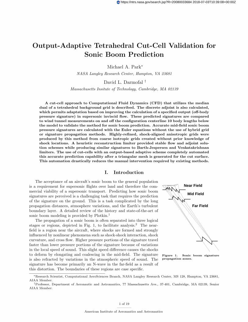
Figure 1. Sonic boom signaturepropagation zones.

The acceptance of an aircraft’s sonic boom to the general populationis a requirement for supersonic flights over land and therefore the com-mercial viability of a supersonic transport. Predicting how sonic boomsignatures are perceived is a challenging task that requires the predictionof the signature on the ground. This is a task complicated by the longpropagation distances, atmosphere variations, and the Earth’s turbulentboundary layer. A detailed review of the history and state-of-the-art ofsonic boom modeling is provided by Plotkin.1

The propagation of a sonic boom is often separated into three logicalstages or regions, depicted in Fig. 1, to facilitate analysis.2 The near-field is a region near the aircraft, where shocks are formed and stronglyinfluenced by nonlinear phenomena such as shock-shock interaction, shockcurvature, and cross flow. Higher pressure portions of the signature travelfaster than lower pressure portions of the signature because of variationsin the local speed of sound. This slight speed difference causes the shocksto deform by elongating and coalescing in the mid-field. The signatureis also refracted by variations in the atmospheric speed of sound. Thesignature has become primarily an N-wave in the far-field as a result ofthis distortion. The boundaries of these regions are case specific.

∗Research Scientist, Computational AeroSciences Branch, NASA Langley Research Center, MS 128, Hampton, VA 23681,AIAA Member.

†Professor, Department of Aeronautic and Astronautics, 77 Massachusetts Ave., 37-401, Cambridge, MA 02139, SeniorAIAA Member.

1 of 19

American Institute of Aeronautics and Astronautics

https://ntrs.nasa.gov/search.jsp?R=20080033684 2018-07-03T10:39:08+00:00Z

Whitham3,4 provides analytic solutions for the signal distortion of slender axisymmetric projectiles.Boom propagation has been implemented in a number of computer programs.5,6 Unfortunately, these boompropagation methods are not directly applicable to complex aircraft geometries. Page and Plotkin7 appliedthe multipoles of George8 to combine CFD near-field calculation with mid- and far-field boom propagation.This CFD matching multipole propagation technique has been revisited by Rallabhandi and Mavris.9

CFD codes have difficulty propagating the relatively weak pressure signatures of a sonic boom to distancesbeyond the near-field region, where these boom propagation methods are valid. This problem is more acutefor unstructured grid methods that are often employed to capture the geometrical complexity of the model,especially if the grids are not aligned with the shocks. To improve alignment, isotropic unstructured grids arestretched to align the tetrahedra with the free stream Mach angle to improve signal propagation for initialgrids.10 This alignment issue has also given rise to hybrid methods11–13 where near-body unstructuredgrid solutions are interpolated to shock-aligned structured grid methods to increase accuracy. The hybridmethods are hindered by the interpolation process, so adaptive grid methods14,15 are employed to improvethe accuracy of unstructured grid methods for long propagation distances. These previous adaptive methodshave used only primal solution information (Mach and density) to drive the adaptive process.

Adaptive grid methods are designed to specify a resolution request that equidistributes and minimizeserror estimates. The improved resolution request is commonly based on local error estimates.16–18 Uniformlyreducing the errors associated with all local-error sources of the flow may not be optimal from an engineeringcontext, where calculating an output functional (i.e., boom signature) may be of greater concern. Analternative method is to estimate the error in the calculation of a specified engineering output functional.19–22

Output error indicators utilize the dual or adjoint solution of an output functional to account for the impactof local error as well as the transport of these local errors throughout the problem domain to improvethe calculation of that output functional. This output-adaptive approach has been applied to sonic boomprediction in 2D with discontinuous Galerkin23,24 and Cartesian methods.22

In this work, anisotropic output-based adaptation to improve an off-body pressure integral is appliedto 3D sonic boom prediction. Anisotropically adapted tetrahedral background grids with cut-cells provideextremely robust adaptation mechanics, enabling the automated application of anisotropic output-basedadaptation to non-trivial 3D sonic boom problems for the first time. This allows for the entire signature tobe calculated or the pressure integral can be restricted to a specific region of interest. The adjoint solutioncan also provide engineering intuition with a rigorous foundation for design sensitivities25 and discretizationerror estimates.21

Cut-cell methods with Cartesian background grids26–29 have been very successful for Euler simulations.The regular structure of the Cartesian background grid permits extremely efficient solution schemes. Carte-sian background grids have the capability to only provide anisotropic resolution in the Cartesian directions.29

Simplex meshes have the ability to stretch the triangular and tetrahedral elements in arbitrary directions.This permits the efficient representation of anisotropic features (i.e., shocks). The cut-cell method is alsoapplicable to simplex meshes.30–32 When the constraint of providing a body-fitted grid is removed, the gridadaptation task becomes much simpler. The complexities of adaptation on curved domain boundaries33 iseliminated and robustness is dramatically increased.

The 3D anisotropic output-adaptive method for sonic boom prediction has previously been applied tobody-fitted grids.34,35 This work addresses two of the weaknesses uncovered in the previous work: adjointiterative convergence for reconstruction limiters and the robustness of body-fitted adaptive mechanics. Thecurrent method is validated by comparison to wind tunnel data for representative configurations.

II. Cut-Cell Determination

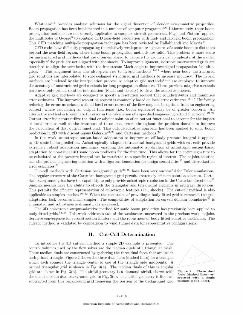
Figure 2. Three dualfaces (dashed lines) as-sociated with a singletriangle (solid lines).

To introduce the 3D cut-cell method a simple 2D example is presented. Thecontrol volumes used by the flow solver are the median duals of a triangular mesh.These median duals are constructed by gathering the three dual faces that are insideeach primal triangle. Figure 2 shows the three dual faces (dashed lines) for a triangle,which each connect the triangle center to one of the triangle side midpoints. Aprimal triangular grid is shown in Fig. 3(a). The median duals of this triangulargrid are shown in Fig. 3(b). The airfoil geometry is a diamond airfoil, shown withthe uncut median dual background grid in Fig. 3(c). The airfoil geometry is Booleansubtracted from this background grid removing the portion of the background grid

2 of 19


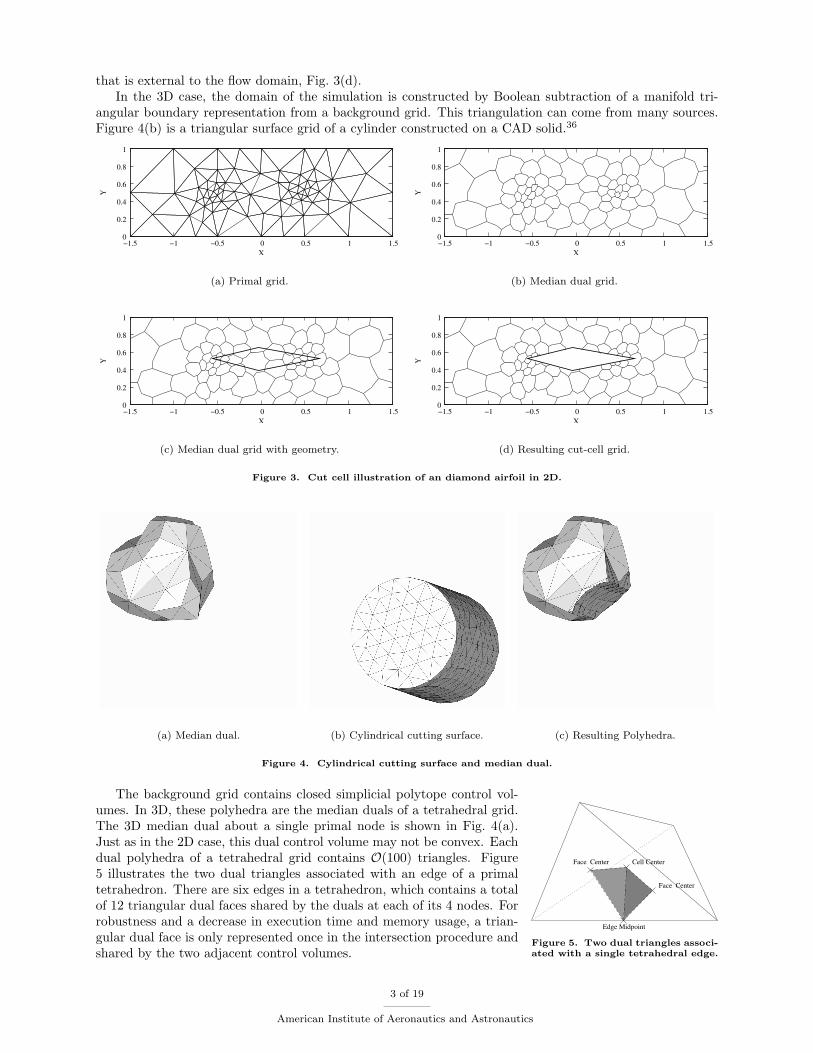
that is external to the flow domain, Fig. 3(d).In the 3D case, the domain of the simulation is constructed by Boolean subtraction of a manifold tri-

angular boundary representation from a background grid. This triangulation can come from many sources.Figure 4(b) is a triangular surface grid of a cylinder constructed on a CAD solid.36

0

0.2

0.4

0.6

0.8

1

−1.5 −1 −0.5 0 0.5 1 1.5

Y

X

(a) Primal grid.

0

0.2

0.4

0.6

0.8

1

−1.5 −1 −0.5 0 0.5 1 1.5

Y

X

(b) Median dual grid.

0

0.2

0.4

0.6

0.8

1

−1.5 −1 −0.5 0 0.5 1 1.5

Y

X

(c) Median dual grid with geometry.

0

0.2

0.4

0.6

0.8

1

−1.5 −1 −0.5 0 0.5 1 1.5Y

X

(d) Resulting cut-cell grid.

Figure 3. Cut cell illustration of an diamond airfoil in 2D.

(a) Median dual. (b) Cylindrical cutting surface. (c) Resulting Polyhedra.

Figure 4. Cylindrical cutting surface and median dual.

Face Center

Face Center Cell Center

Edge Midpoint

Figure 5. Two dual triangles associ-ated with a single tetrahedral edge.

The background grid contains closed simplicial polytope control vol-umes. In 3D, these polyhedra are the median duals of a tetrahedral grid.The 3D median dual about a single primal node is shown in Fig. 4(a).Just as in the 2D case, this dual control volume may not be convex. Eachdual polyhedra of a tetrahedral grid contains O(100) triangles. Figure5 illustrates the two dual triangles associated with an edge of a primaltetrahedron. There are six edges in a tetrahedron, which contains a totalof 12 triangular dual faces shared by the duals at each of its 4 nodes. Forrobustness and a decrease in execution time and memory usage, a trian-gular dual face is only represented once in the intersection procedure andshared by the two adjacent control volumes.

3 of 19


Aftosmis, Berger, and Melton28 demonstrate a method to perform theBoolean subtraction of two manifold triangular polyhedra (surface grid and each of the background gridcontrol volumes) with a series of triangle-triangle intersections. Their methodology was modified to use onlyfloating point arithmetic by Park.37 The result of this subtraction is shown in Fig. 4(c).

III. Flow and Adjoint Solvers

Fully Unstructured Navier-Stokes Three-Dimensional (FUN3D) is a suite of codes for finite-volumeCFD.38 The FUN3D website, http://fun3d.larc.nasa.gov, contains the user manual and an extensive listof references. FUN3D is able to solve incompressible, Euler, and Reynolds-averaged Navier-Stokes (RANS)flow equations, either tightly or loosely coupled to a turbulence model. The Euler equations are used in thisstudy. Domain decomposition is employed to fully exploit the distributed memory of a cluster of computersto increase problem size and reduce the execution time of the simulation process.

The Euler equations are∂Q∂t

+∇ · F = 0, (1)

Q =

ρ

ρu

ρv

ρw

E

, F =

ρu

ρu2 + p

ρuv

ρuw

u(p + E)

i +

ρv

ρvu

ρv2 + p

ρvw

v(p + E)

j +

ρw

ρwu

ρwv

ρw2 + p

w(p + E)

k, (2)

where ρ is density, u, v, and w are velocity, E is total energy per unit volume, and p is pressure. Thesequantities are related by the ideal gas relation,

p = (γ − 1)(

E − ρu2 + v2 + w2

2

), (3)

with the specific heat ratio γ = 1.4 for air.The divergence theorem is applied over a set of control volumes to produce a finite-volume scheme,∫

Vi

(∂Q∂t

+∇ · F)

dV = VidQi

dt+

∫Γi

F · ~n dΓ = 0, (4)

where Γi are the boundaries of the control volumes with volume Vi and ~n is an outward pointing normal.The average of Q in each control volume is Qi. The flux integration is approximated as,∫

Γi

F · ~n dΓ ≈∑f∈Γi

H(qlf , qrf , ~nf )Af = Ri(Q), (5)

where Ri is the discrete residual for control volume i, the summation is over the faces of the control volume.38

The van Leer39 approximate Riemann solver H is utilized to compute the flux from the primitive states,

q =[

ρ u v w p]T

, (6)

at the borders of the neighboring control volumes, qrf and qlf . These face values are reconstructed from cellaverages (the reconstruction method is described below). The discrete equations are established simultane-ously for each control volume,

VdQ

dt+ R(Q) = 0, (7)

which makes the discrete solution vector Q ∈ R5N , discrete residual vector R ∈ R5N , and V = diag(Vi),where N is the number of control volumes. The flux integration scheme (including face state reconstructionfrom cell averages) is detailed in the following sections.

A backward Euler solution update scheme is employed with a variable pseudo-time step.38 An approxi-mate nearest neighbor linearization is utilized to reduce the memory required for the implicit point-iterativemethod. After the flow solution is known, the discrete adjoint equations25,40 are solved to complete thedual problem. The linear adjoint equations are solved with a dual-consistent time-marching method.41,42

The dual-consistent solution method guarantees that the adjoint equations will have the same asymptoticconvergence rate as the flow equations.

4 of 19


III.A. Inviscid Flux Integration

The existing FUN3D body-fitted approach lumps the median dual pieces to a single effective area and normaldirection for each edge they surround.43 After lumping, all of the inviscid terms are calculated with a loopover edges, which is computationally efficient. Conserved states Q, used in the time advancement scheme,are converted to primitive states q for face state reconstruction. The primitive state is extrapolated fromthe nodes to establish the primitive state at these lumped faces qf using the gradients ∇q = [qx, qy, qz], facecenter xf , and node x0,

qf = q0 +∇q (xf − x0), (8)

for the unlimited scheme. The gradient is reconstructed from the cell averaged state q0 with a weighted leastsquares method, see Park37 for details. For the case of supersonic flow, a limiting function is used to reducethe gradient contribution to the reconstruction (see Subsection III.B).

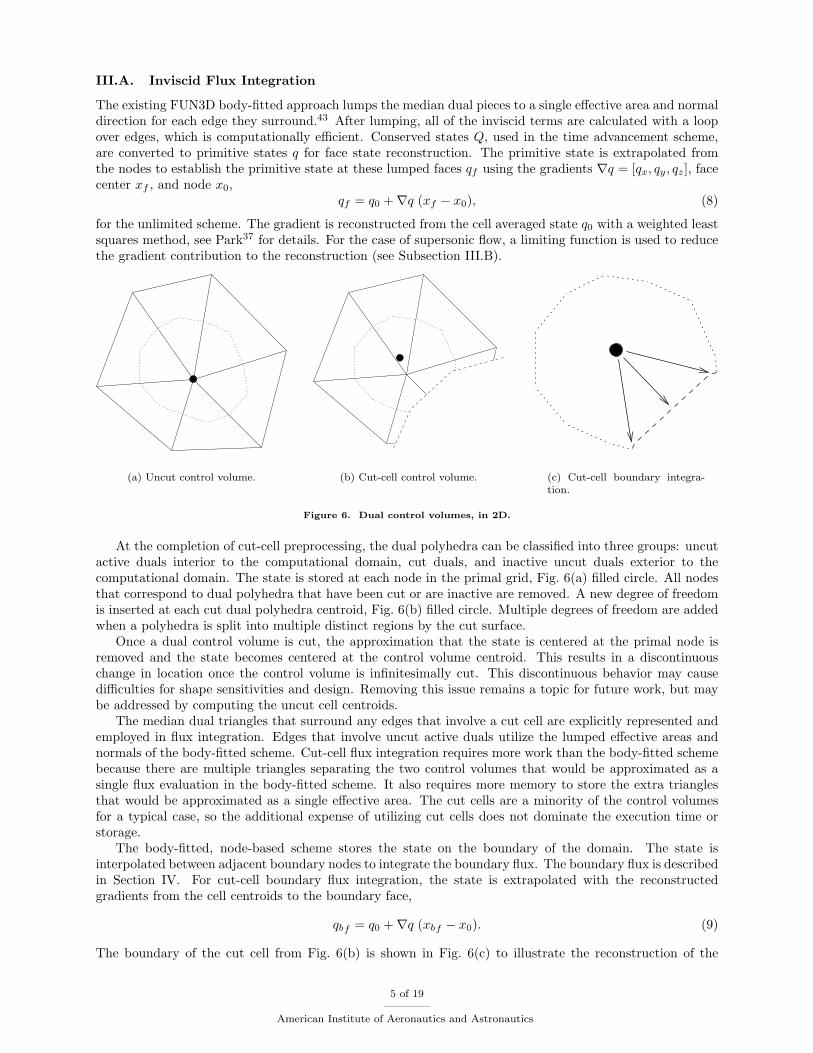
(a) Uncut control volume. (b) Cut-cell control volume. (c) Cut-cell boundary integra-tion.

Figure 6. Dual control volumes, in 2D.

At the completion of cut-cell preprocessing, the dual polyhedra can be classified into three groups: uncutactive duals interior to the computational domain, cut duals, and inactive uncut duals exterior to thecomputational domain. The state is stored at each node in the primal grid, Fig. 6(a) filled circle. All nodesthat correspond to dual polyhedra that have been cut or are inactive are removed. A new degree of freedomis inserted at each cut dual polyhedra centroid, Fig. 6(b) filled circle. Multiple degrees of freedom are addedwhen a polyhedra is split into multiple distinct regions by the cut surface.

Once a dual control volume is cut, the approximation that the state is centered at the primal node isremoved and the state becomes centered at the control volume centroid. This results in a discontinuouschange in location once the control volume is infinitesimally cut. This discontinuous behavior may causedifficulties for shape sensitivities and design. Removing this issue remains a topic for future work, but maybe addressed by computing the uncut cell centroids.

The median dual triangles that surround any edges that involve a cut cell are explicitly represented andemployed in flux integration. Edges that involve uncut active duals utilize the lumped effective areas andnormals of the body-fitted scheme. Cut-cell flux integration requires more work than the body-fitted schemebecause there are multiple triangles separating the two control volumes that would be approximated as asingle flux evaluation in the body-fitted scheme. It also requires more memory to store the extra trianglesthat would be approximated as a single effective area. The cut cells are a minority of the control volumesfor a typical case, so the additional expense of utilizing cut cells does not dominate the execution time orstorage.

The body-fitted, node-based scheme stores the state on the boundary of the domain. The state isinterpolated between adjacent boundary nodes to integrate the boundary flux. The boundary flux is describedin Section IV. For cut-cell boundary flux integration, the state is extrapolated with the reconstructedgradients from the cell centroids to the boundary face,

qbf = q0 +∇q (xbf − x0). (9)

The boundary of the cut cell from Fig. 6(b) is shown in Fig. 6(c) to illustrate the reconstruction of the

5 of 19


boundary state qbf for cut-cell boundary flux integration. The qbf is extrapolated to each cut surface piecefor integration.

III.B. Reconstruction Limiting

Barth and Jespersen43 introduced limits on an unstructured grid reconstruction scheme to maintain mono-tonicity. Face reconstruction using a limiter of this form is

qf = q0 + Φ ∇q (xf − x0), (10)

where the diagonal matrix limiting function Φ is computed in each control volume. The same Φ is employedin all face reconstructions for a given control volume. This type of limiter can compromise the convergence ofthe flow solution and therefore a dual-consistent adjoint solver.44,45 Venkatakrishnan46 studied this limiterin its original form as well as with the limiter function held constant (i.e. frozen) after iterative convergencestalls. He proposed a new limiter to improve convergence, but both the frozen scheme and new limiter canresult in stalled convergence. The Venkatakrishnan limiter is not monotone, it permits under- and over-shoots. Frozen limiters are approximations that impede error estimation, output-based adaptation, adjointiterative convergence, and design sensitivities.22,34,47

In this study, the limiter will be used in the context of an output adaptive scheme that requires theadjoint solution. An exact linearization and steady iterative convergence of the flow and adjoint solversis paramount to the robustness of the adaptive scheme. This iterative convergence is so critical that theaccuracy of the limited scheme will be sacrificed; accuracy will be regained with adaptive grid refinementand alignment. A heuristic edge-based limiter48 is utilized to improve the convergence of the flow solverwhile providing the exact linearization required for adjoint convergence. Concessions are made to improveiterative convergence; it is not total variation diminishing (TVD) or linearity preserving.

The heuristic limiter was developed48 by examining its effect on shock capturing for regular and irregulargrids and empirically adjusting its formulation to increase the width of shocks. It is a scalar limitingfunction φ that considers only the cell-averaged values of pressure and their reconstructed gradients in thecells adjacent to the face being reconstructed. Face reconstruction using a limiter of this form is

qf = q + φ∇q(xf − x0), (11)

where the scalar limiting function φ is computed for each face f . The same φ is used for the left qlf andright qrf face reconstructions.

Face

EdgeFace Center

xδ 1

δx2

p1

p2

Figure 7. Edge and face geometry.

The basic concept employed in this heuristic limiter is to reduce the reconstruction gradient in locationswhere the pressure gradients are large relative to pressure. This clearly could result in limiting in regions forwhich the solution varies linearly (though with large magnitude), however, in combination with adaptationthe proposed limiter has been found robust and accurate. The specific form of the limiter relies on a measureof the change in the pressure, δp. To form δp, the reconstructed gradient of pressure for the control volumeson the right and left of the face (Fig. 7), ∇p1 and ∇p2, are used with the right and left extrapolation vectorsto the face, δx1 and δx2,

δp =

∣∣∣∣∣∣∣∣∣∣∣∣∣∣

δx1x∇p1x

− δx2x∇p2x

δx1y∇p1y

− δx2y∇p2y

δx1z∇p1z

− δx2z∇p2z

∣∣∣∣∣∣∣∣∣∣∣∣∣∣ . (12)

This sensor is active for linear functions and does not specifically penalize extrema. The gradient recon-struction is reduced where the the δp sensor is large with the intention of spreading the detected jump over

6 of 19


a number of control volumes. Adaptation will be employed to narrow the width of the discontinuity. Thetanh function is employed to smooth the combined nondimensional pressure jump ratio,

φheuristic = 1− tanh(

δp

min(p1, p2)

), (13)

and restricts the limiter to the range (0, 1]. A tanh function is employed to provide a smoothly varyingand differentiable function that enables residual convergence that can be impeded by a non-smooth limitingfunction. This limiter is active (to some degree) in all regions with pressure variations, so it will not switchon and off intermittently during iterative convergence. The design accuracy of the limited scheme is thereforebelow second-order. The limiter is more active when the pressure variation is significant as compared to thelocal pressure.

The cut cells require pressure extrapolated to the boundaries to compute boundary fluxes. This recon-struction requires limiting to prevent unrealizable face states and must be smoothly differentiable to facilitateiterative convergence,

δpd =

∣∣∣∣∣∣∣∣∣∣∣∣∣∣

δxx∇px

δxy∇py

δxz∇pz

∣∣∣∣∣∣∣∣∣∣∣∣∣∣ , (14)

φextrapolation = 1− tanh(

δp

p

). (15)

The extrapolation limiter is formulated to mimic the interior face limiter using only the data from the celladjacent to the boundary.

IV. Boundary Conditions

The boundary conditions are imposed weakly through the fluxes. The tangential flow boundary conditionis implemented with zero velocity normal to the boundary, resulting in the flux,

Ftangential =

0

pnx

pny

pnz

0

, (16)

where p is interpolated along or extrapolated to the boundary. The supersonic outflow boundary conditionuses the interior state to form the boundary flux. The supersonic inflow boundary condition uses the freestream state ρ∞, u∞, v∞, w∞, and p∞ to form the boundary flux.

The inviscid flow model breaks down at a sharp corner where separation would occur in a physical flow.In the supersonic flow simulations performed in this work, this problem presents itself at blunt trailingedges. To avoid this problem in these regions, a transpiration boundary condition is specified manually.This boundary condition applies free stream velocity state, u∞, v∞, and w∞ with a density and pressure ofρ = 0.3ρ∞ and p = 0.3p∞. This level of density and pressure is empirically established by examining thesolution of a backward facing step with the tangential boundary condition.

V. Output-Based Adaptation

Venditti21 describes an output-based error estimation and adaptation scheme. To formulate the errorestimate, an embedded grid is required. Constructing the entire embedded grid can be infeasible for large3D grids and has prevented the use of adjoint error estimation techniques for industrial-sized problems evenwith a parallel implementation.34 While the embedded grid can be formed in sections, this increases theerror estimation scheme complexity. Forming a portion or the entire embedded grid is also complicated bythe need to respect curved boundaries and recompute the intersection tests of cut cells. These difficultieshave motivated the desire to employ only the current grid in the error estimation procedure. A procedure

7 of 19


is described that obtains an indicator for output adaptation with the current grid, but does not provide afunctional error correction.

Park37 provides a derivation of the single-grid adaptive indicator by placing it in the context of theembedded grid approach of Venditti. In the interest of brevity, the single-grid error estimation and adaptiveindicator is provided without a derivation,

[Isingle]κ =12

5∑i=1

∣∣∣[Rλ(λ)]i,κ[Q− Q]i,κ∣∣∣ +

∣∣∣[λ− λ]i,κ[R(Q)]i,κ∣∣∣ . (17)

It has the same pieces as the Venditti error indicator, where the five conservation equations are contractedby the summation over i. The vector Isingle ∈ RN has a single value for each grid control volume κ. Theλ and Q higher-order reconstructions and the λ, and Q lower-order reconstructions on the current grid aredescribed in Park.37 The original residual operators are utilized and λ and Q are constructed to make Rλ(λ)and R(Q) reliable adaptive indicators. The λ and Q reconstructions are formed with a fit of quadraticfunctions to cell averaged states and their gradients. The difference between the () and () reconstructions isintended to provide adequate guidance for the relative distribution of error, not a sharp bound on error.

Venditti21 provides a procedure to calculate a new grid spacing request h from the adaptive indicatorIκ and an error tolerance tolΩ. The adjoint adaptation parameter was also incorporated into an anisotropicHessian-based framework. This combined approach sets the anisotropy of mesh elements by using the MachHessian, and it scales the element size so that the tightest spacing is dictated by the adjoint adaptationparameter. The metric-based grid mechanics is described by Park and Darmofal.37,49 It is fully parallelizedand interfaces directly with the error estimation process.

VI. Application to Sonic Boom Prediction

The parallel metric-based adaptation algorithm is applied to sonic boom prediction. More detailedinformation on these cases, including timing information, is available in Park.37 The output for the adaptiveprocedure of the integral of quadratic pressure deviation over a surface s in the domain,

f =1

As

∫∫s

(p− p∞

p∞

)2

ds, (18)

where As is the area of the integration surface. This focuses the adaptation on improving the calculationof pressure near this surface. Previous applications have been performed with the integral of pressuredeviation.34,35 However, the square of this deviation has been shown to produce more accurate signatureswith less control volumes.22 A cylindrical integration surface, aligned to the x-axis, is employed. The extentof the integration surface can be optionally restricted to the interior of a box to focus on a subsection of thecylinder.

The current output-based adaptation approach is validated with wind tunnel measurements. Windtunnel testing of sonic boom configurations is a challenging task. Wind tunnel models are typically smallto obtain pressure signatures a relatively large distance from the model within the finite size of tunnel testsections. Carlson and Morris50 present some of difficulties inherent in wind tunnel testing of these smallmodels including extraneous variations in pressure larger than the signals measured. A test apparatus andprocedure that mitigates the extraneous spatial and temporal distortions is described. Morgenstern51 alsodocuments variations in ambient static pressure wind tunnel measurements that are of the same magnitude

Figure 8. Cone-Cylinder Ge-ometry.

as the desired signature measurement.

VI.A. Cone-Cylinder Configuration

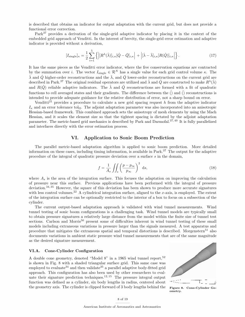
A double cone geometry, denoted “Model 8” in a 1965 wind tunnel report,52

is shown in Fig. 8 with a shaded triangular surface grid. This same case wasemployed to evaluate34 and then validate35 a parallel adaptive body-fitted gridapproach. This configuration has also been used by other researchers to eval-uate their signature prediction techniques.12,15 The pressure integral outputfunction was defined as a cylinder, six body lengths in radius, centered aboutthe geometry axis. The cylinder is clipped forward of 3 body lengths behind the

8 of 19


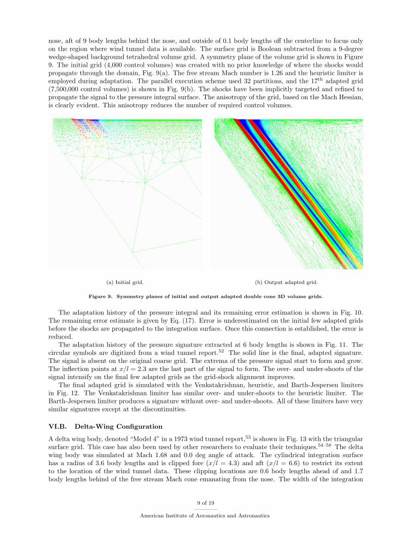
nose, aft of 9 body lengths behind the nose, and outside of 0.1 body lengths off the centerline to focus onlyon the region where wind tunnel data is available. The surface grid is Boolean subtracted from a 9-degreewedge-shaped background tetrahedral volume grid. A symmetry plane of the volume grid is shown in Figure9. The initial grid (4,000 control volumes) was created with no prior knowledge of where the shocks wouldpropagate through the domain, Fig. 9(a). The free stream Mach number is 1.26 and the heuristic limiter isemployed during adaptation. The parallel execution scheme used 32 partitions, and the 17th adapted grid(7,500,000 control volumes) is shown in Fig. 9(b). The shocks have been implicitly targeted and refined topropagate the signal to the pressure integral surface. The anisotropy of the grid, based on the Mach Hessian,is clearly evident. This anisotropy reduces the number of required control volumes.

(a) Initial grid. (b) Output adapted grid.

Figure 9. Symmetry planes of initial and output adapted double cone 3D volume grids.

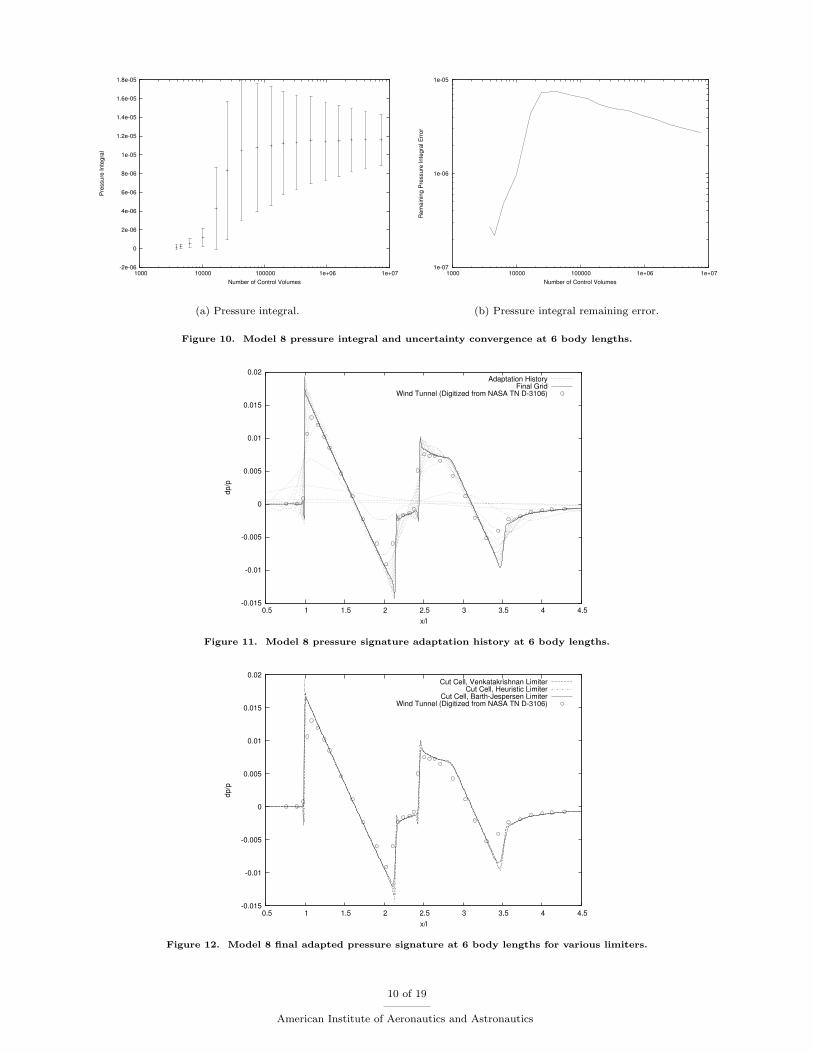
The adaptation history of the pressure integral and its remaining error estimation is shown in Fig. 10.The remaining error estimate is given by Eq. (17). Error is underestimated on the initial few adapted gridsbefore the shocks are propagated to the integration surface. Once this connection is established, the error isreduced.

The adaptation history of the pressure signature extracted at 6 body lengths is shown in Fig. 11. Thecircular symbols are digitized from a wind tunnel report.52 The solid line is the final, adapted signature.The signal is absent on the original coarse grid. The extrema of the pressure signal start to form and grow.The inflection points at x/l = 2.3 are the last part of the signal to form. The over- and under-shoots of thesignal intensify on the final few adapted grids as the grid-shock alignment improves.

The final adapted grid is simulated with the Venkatakrishnan, heuristic, and Barth-Jespersen limitersin Fig. 12. The Venkatakrishnan limiter has similar over- and under-shoots to the heuristic limiter. TheBarth-Jespersen limiter produces a signature without over- and under-shoots. All of these limiters have verysimilar signatures except at the discontinuities.

VI.B. Delta-Wing Configuration

A delta wing body, denoted “Model 4” in a 1973 wind tunnel report,53 is shown in Fig. 13 with the triangularsurface grid. This case has also been used by other researchers to evaluate their techniques.54–58 The deltawing body was simulated at Mach 1.68 and 0.0 deg angle of attack. The cylindrical integration surfacehas a radius of 3.6 body lengths and is clipped fore (x/l = 4.3) and aft (x/l = 6.6) to restrict its extentto the location of the wind tunnel data. These clipping locations are 0.6 body lengths ahead of and 1.7body lengths behind of the free stream Mach cone emanating from the nose. The width of the integration

9 of 19


-2e-06

0

2e-06

4e-06

6e-06

8e-06

1e-05

1.2e-05

1.4e-05

1.6e-05

1.8e-05

1000 10000 100000 1e+06 1e+07

Pres

sure

Inte

gral

Number of Control Volumes

(a) Pressure integral.

1e-07

1e-06

1e-05

1000 10000 100000 1e+06 1e+07

Rem

aini

ng P

ress

ure

Inte

gral

Erro

r


(b) Pressure integral remaining error.

Figure 10. Model 8 pressure integral and uncertainty convergence at 6 body lengths.

-0.015

-0.01

-0.005

0

0.005

0.01

0.015

0.02

0.5 1 1.5 2 2.5 3 3.5 4 4.5

dp/p

x/l

Adaptation HistoryFinal Grid

Wind Tunnel (Digitized from NASA TN D-3106)

Figure 11. Model 8 pressure signature adaptation history at 6 body lengths.

-0.015

-0.01

-0.005

0

0.005

0.01

0.015

0.02

0.5 1 1.5 2 2.5 3 3.5 4 4.5

dp/p

x/l

Cut Cell, Venkatakrishnan LimiterCut Cell, Heuristic Limiter

Cut Cell, Barth-Jespersen LimiterWind Tunnel (Digitized from NASA TN D-3106)

Figure 12. Model 8 final adapted pressure signature at 6 body lengths for various limiters.

10 of 19


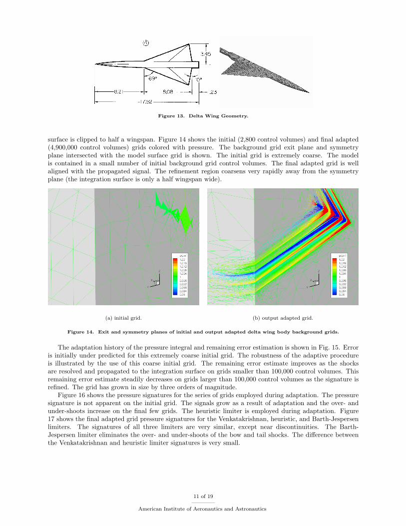
Figure 13. Delta Wing Geometry.

surface is clipped to half a wingspan. Figure 14 shows the initial (2,800 control volumes) and final adapted(4,900,000 control volumes) grids colored with pressure. The background grid exit plane and symmetryplane intersected with the model surface grid is shown. The initial grid is extremely coarse. The modelis contained in a small number of initial background grid control volumes. The final adapted grid is wellaligned with the propagated signal. The refinement region coarsens very rapidly away from the symmetryplane (the integration surface is only a half wingspan wide).

(a) initial grid. (b) output adapted grid.

Figure 14. Exit and symmetry planes of initial and output adapted delta wing body background grids.

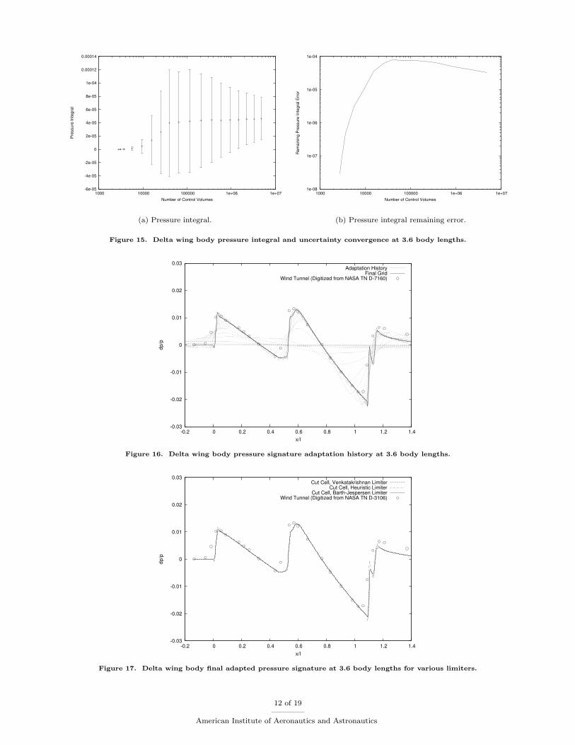
The adaptation history of the pressure integral and remaining error estimation is shown in Fig. 15. Erroris initially under predicted for this extremely coarse initial grid. The robustness of the adaptive procedureis illustrated by the use of this coarse initial grid. The remaining error estimate improves as the shocksare resolved and propagated to the integration surface on grids smaller than 100,000 control volumes. Thisremaining error estimate steadily decreases on grids larger than 100,000 control volumes as the signature isrefined. The grid has grown in size by three orders of magnitude.

Figure 16 shows the pressure signatures for the series of grids employed during adaptation. The pressuresignature is not apparent on the initial grid. The signals grow as a result of adaptation and the over- andunder-shoots increase on the final few grids. The heuristic limiter is employed during adaptation. Figure17 shows the final adapted grid pressure signatures for the Venkatakrishnan, heuristic, and Barth-Jespersenlimiters. The signatures of all three limiters are very similar, except near discontinuities. The Barth-Jespersen limiter eliminates the over- and under-shoots of the bow and tail shocks. The difference betweenthe Venkatakrishnan and heuristic limiter signatures is very small.

11 of 19


-6e-05

-4e-05

-2e-05

0

2e-05

4e-05

6e-05

8e-05

1e-04

0.00012

0.00014

1000 10000 100000 1e+06 1e+07

Pres

sure

Inte

gral



1e-08

1e-07

1e-06

1e-05

1e-04

1000 10000 100000 1e+06 1e+07

Rem

aini

ng P

ress

ure

Inte

gral

Erro

r



Figure 15. Delta wing body pressure integral and uncertainty convergence at 3.6 body lengths.

-0.03

-0.02

-0.01

0

0.01

0.02

0.03

-0.2 0 0.2 0.4 0.6 0.8 1 1.2 1.4

dp/p

x/l

Adaptation HistoryFinal Grid

Wind Tunnel (Digitized from NASA TN D-7160)

Figure 16. Delta wing body pressure signature adaptation history at 3.6 body lengths.

-0.03

-0.02

-0.01

0

0.01

0.02

0.03

-0.2 0 0.2 0.4 0.6 0.8 1 1.2 1.4

dp/p

x/l


Cut Cell, Barth-Jespersen LimiterWind Tunnel (Digitized from NASA TN D-3106)

Figure 17. Delta wing body final adapted pressure signature at 3.6 body lengths for various limiters.

12 of 19


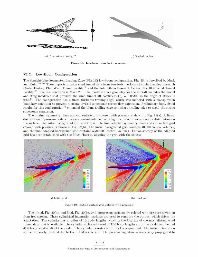
(a) Three-view drawing.59 (b) Shaded Surface.

Figure 18. Low-boom wing body geometry.

VI.C. Low-Boom Configuration

The Straight-Line Segmented Leading Edge (SLSLE) low-boom configuration, Fig. 18, is described by Mackand Kuhn.59,60 These reports provide wind tunnel data from two tests, performed at the Langley ResearchCenter Unitary Plan Wind Tunnel Facility59 and the John Glenn Research Center 10× 10 ft Wind TunnelFacility.60 The test condition is Mach 2.0. The model surface geometry for the aircraft includes the modeland sting incidence that provides the wind tunnel lift coefficient CL = 0.08309 so the angle of attack iszero.11 The configuration has a finite thickness trailing edge, which was modeled with a transpirationboundary condition to prevent a strong inviscid supersonic corner flow expansion. Preliminary body-fittedresults for this configuration34 extended the blunt trailing edge to a sharp trailing edge to avoid the strongsupersonic expansion.

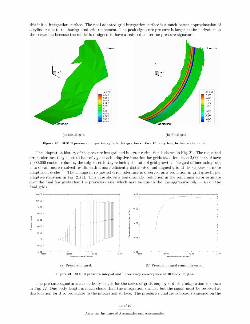
The original symmetry plane and cut surface grid colored with pressure is shown in Fig. 19(a). A lineardistribution of pressure is shown in each control volume, resulting in a discontinuous pressure distribution onthe surface. The initial background grid is isotropic. The final adapted symmetry plane and cut surface gridcolored with pressure is shown in Fig. 19(b). The initial background grid contains 40,000 control volumes,and the final adapted background grid contains 5,700,000 control volumes. The anisotropy of the adaptedgrid has been established with the Mach Hessian, aligning the grid with the shocks.

(a) Initial grid. (b) Final grid.

Figure 19. SLSLE surface grid colored with pressure.

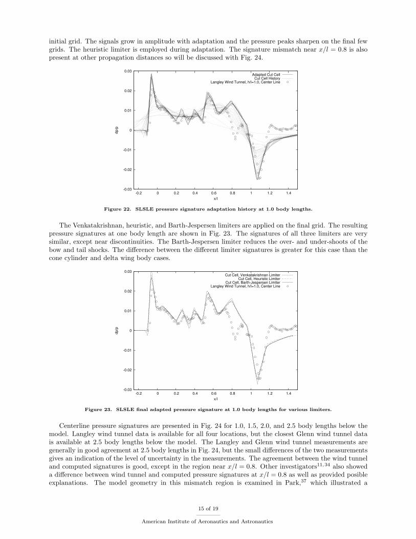
The initial, Fig. 20(a), and final, Fig. 20(b), grid integration surfaces are colored with pressure deviationfrom free stream. These cylindrical integration surfaces are used to compute the output, which drives theadaptation. The cylinder has a radius of 10 body lengths, which is the location of the most distant windtunnel data that is available. The cylinder is clipped ahead of 32.6 body lengths aft of the model and behind41.0 body lengths aft of the model. The cylinder is restricted to its lower quadrant. The initial integrationsurface is poorly resolved due to the initial coarse grid. The pressure signature is not visibly propagated to

13 of 19


this initial integration surface. The final adapted grid integration surface is a much better approximation ofa cylinder due to the background grid refinement. The peak signature pressure is larger at the horizon thanthe centerline because the model is designed to have a reduced centerline pressure signature.

(a) Initial grid. (b) Final grid.

Figure 20. SLSLE pressure on quarter cylinder integration surface 10 body lengths below the model.

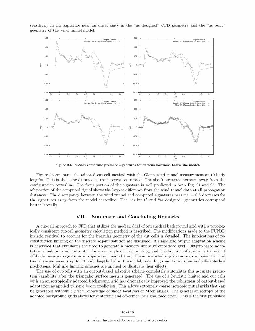
The adaptation history of the pressure integral and its error estimation is shown in Fig. 21. The requestederror tolerance tolΩ is set to half of IΩ at each adaptive iteration for grids sized less than 2,000,000. Above2,000,000 control volumes, the tolΩ is set to IΩ, reducing the rate of grid growth. The goal of increasing tolΩis to obtain more resolved results with a more efficiently distributed and aligned grid at the expense of moreadaptation cycles.31 The change in requested error tolerance is observed as a reduction in grid growth peradaptive iteration in Fig. 21(a). This case shows a less dramatic reduction in the remaining error estimateover the final few grids than the previous cases, which may be due to the less aggressive tolΩ = IΩ on thefinal grids.

-4e-06

-2e-06

0

2e-06

4e-06

6e-06

8e-06

1e-05

1.2e-05

1.4e-05

10000 100000 1e+06 1e+07

Pres

sure

Inte

gral



1e-09

1e-08

1e-07

1e-06

1e-05

10000 100000 1e+06 1e+07

Rem

aini

ng P

ress

ure

Inte

gral

Erro

r



Figure 21. SLSLE pressure integral and uncertainty convergence at 10 body lengths.

The pressure signatures at one body length for the series of grids employed during adaptation is shownin Fig. 22. One body length is much closer than the integration surface, but the signal must be resolved atthis location for it to propagate to the integration surface. The pressure signature is broadly smeared on the

14 of 19


initial grid. The signals grow in amplitude with adaptation and the pressure peaks sharpen on the final fewgrids. The heuristic limiter is employed during adaptation. The signature mismatch near x/l = 0.8 is alsopresent at other propagation distances so will be discussed with Fig. 24.

-0.03

-0.02

-0.01

0

0.01

0.02

0.03

-0.2 0 0.2 0.4 0.6 0.8 1 1.2 1.4

dp/p

x/l

Adapted Cut CellCut Cell History

Langley Wind Tunnel, h/l=1.0, Center Line

Figure 22. SLSLE pressure signature adaptation history at 1.0 body lengths.

The Venkatakrishnan, heuristic, and Barth-Jespersen limiters are applied on the final grid. The resultingpressure signatures at one body length are shown in Fig. 23. The signatures of all three limiters are verysimilar, except near discontinuities. The Barth-Jespersen limiter reduces the over- and under-shoots of thebow and tail shocks. The difference between the different limiter signatures is greater for this case than thecone cylinder and delta wing body cases.

-0.03

-0.02

-0.01

0

0.01

0.02

0.03

-0.2 0 0.2 0.4 0.6 0.8 1 1.2 1.4

dp/p

x/l


Cut Cell, Barth-Jespersen LimiterLangley Wind Tunnel, h/l=1.0, Center Line

Figure 23. SLSLE final adapted pressure signature at 1.0 body lengths for various limiters.

Centerline pressure signatures are presented in Fig. 24 for 1.0, 1.5, 2.0, and 2.5 body lengths below themodel. Langley wind tunnel data is available for all four locations, but the closest Glenn wind tunnel datais available at 2.5 body lengths below the model. The Langley and Glenn wind tunnel measurements aregenerally in good agreement at 2.5 body lengths in Fig. 24, but the small differences of the two measurementsgives an indication of the level of uncertainty in the measurements. The agreement between the wind tunneland computed signatures is good, except in the region near x/l = 0.8. Other investigators11,34 also showeda difference between wind tunnel and computed pressure signatures at x/l = 0.8 as well as provided posibleexplanations. The model geometry in this mismatch region is examined in Park,37 which illustrated a

15 of 19


sensitivity in the signature near an uncertainty in the “as designed” CFD geometry and the “as built”geometry of the wind tunnel model.

-0.03

-0.02

-0.01

0

0.01

0.02

0.03

-0.2 0 0.2 0.4 0.6 0.8 1 1.2 1.4

dp/p

x/l

Adapted Cut CellLangley Wind Tunnel, h/l=1.0, Center Line

-0.03

-0.02

-0.01

0

0.01

0.02

0.03

-0.2 0 0.2 0.4 0.6 0.8 1 1.2 1.4

dp/p

x/l


-0.03

-0.02

-0.01

0

0.01

0.02

0.03

-0.2 0 0.2 0.4 0.6 0.8 1 1.2 1.4

dp/p

x/l


-0.03

-0.02

-0.01

0

0.01

0.02

0.03

-0.2 0 0.2 0.4 0.6 0.8 1 1.2 1.4

dp/p

x/l


Glenn Wind Tunnel, h/l=2.5, Center Line

Figure 24. SLSLE centerline pressure signatures for various locations below the model.

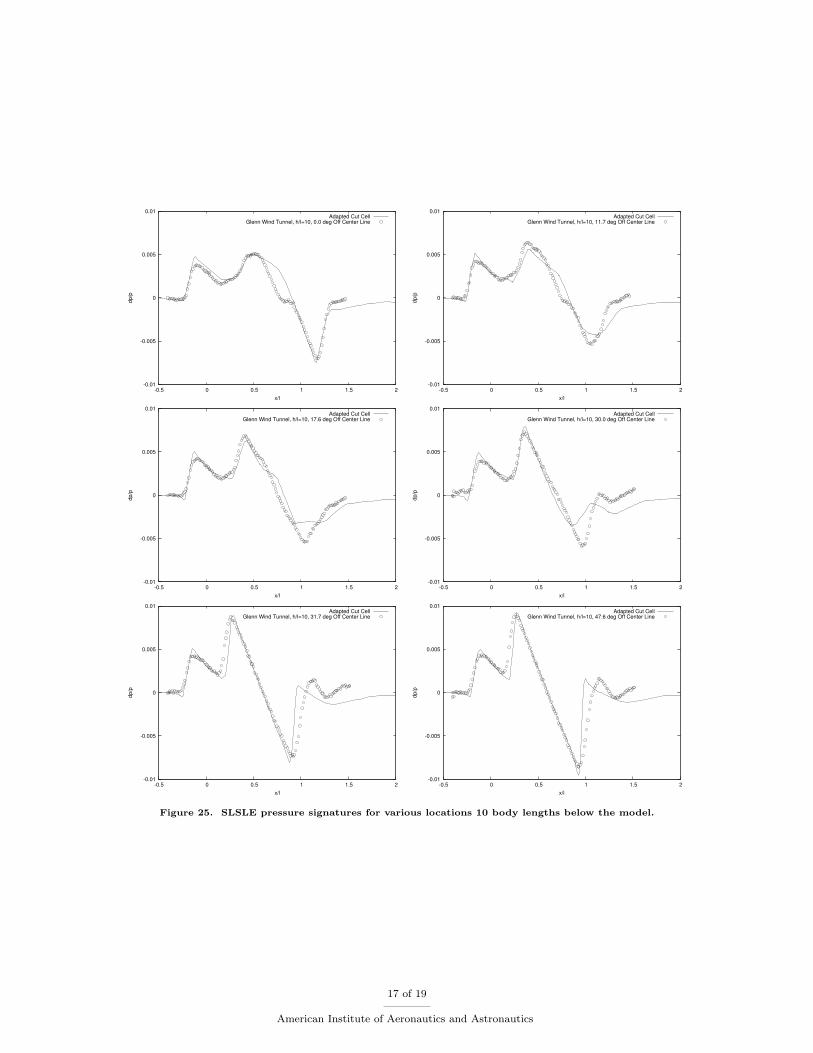
Figure 25 compares the adapted cut-cell method with the Glenn wind tunnel measurement at 10 bodylengths. This is the same distance as the integration surface. The shock strength increases away from theconfiguration centerline. The front portion of the signature is well predicted in both Fig. 24 and 25. Theaft portion of the computed signal shows the largest difference from the wind tunnel data at all propagationdistances. The discrepancy between the wind tunnel and computed signatures near x/l = 0.8 decreases forthe signatures away from the model centerline. The “as built” and “as designed” geometries correspondbetter laterally.

VII. Summary and Concluding Remarks

A cut-cell approach to CFD that utilizes the median dual of tetrahedral background grid with a topolog-ically consistent cut-cell geometry calculation method is described. The modifications made to the FUN3Dinviscid residual to account for the irregular geometry of the cut cells is detailed. The implications of re-construction limiting on the discrete adjoint solution are discussed. A single grid output adaptation schemeis described that eliminates the need to generate a memory intensive embedded grid. Output-based adap-tation simulations are presented for a cone-cylinder, delta wing, and low-boom configurations to predictoff-body pressure signatures in supersonic inviscid flow. These predicted signatures are compared to windtunnel measurements up to 10 body lengths below the model, providing simultaneous on- and off-centerlinepredictions. Multiple limiting schemes are applied to illustrate their effects.

The use of cut-cells with an output-based adaptive scheme completely automates this accurate predic-tion capability after the triangular surface mesh is generated. The use of a heuristic limiter and cut cellswith an anisotropically adapted background grid has dramatically improved the robustness of output-basedadaptation as applied to sonic boom prediction. This allows extremely coarse isotropic initial grids that canbe generated without a priori knowledge of shock locations or Mach angles. The general anisotropy of theadapted background grids allows for centerline and off-centerline signal prediction. This is the first published

16 of 19


-0.01

-0.005

0

0.005

0.01

-0.5 0 0.5 1 1.5 2

dp/p

x/l

Adapted Cut CellGlenn Wind Tunnel, h/l=10, 0.0 deg Off Center Line

-0.01

-0.005

0

0.005

0.01

-0.5 0 0.5 1 1.5 2

dp/p

x/l


-0.01

-0.005

0

0.005

0.01

-0.5 0 0.5 1 1.5 2

dp/p

x/l


-0.01

-0.005

0

0.005

0.01

-0.5 0 0.5 1 1.5 2

dp/p

x/l


-0.01

-0.005

0

0.005

0.01

-0.5 0 0.5 1 1.5 2

dp/p

x/l


-0.01

-0.005

0

0.005

0.01

-0.5 0 0.5 1 1.5 2

dp/p

x/l


Figure 25. SLSLE pressure signatures for various locations 10 body lengths below the model.

17 of 19


CFD prediction of the off-centerline SLSLE signatures at 10 body lengths.

VIII. Acknowledgments

A sincere thank you to Jeffery White for his assistance with shock capturing by providing a limiter thatenables excellent iterative convergence and to Susan Cliff for providing the surface grid of the delta wingconfiguration.

References

1Plotkin, K. J., “State of the art of sonic boom modeling,” The Journal of the Acoustical Society of America, Vol. 111,No. 1, Jan. 2002, pp. 530–536.

2Carlson, H. W., “Experimental and Analytic Research on Sonic Boom Generation at NASA,” Sonic Boom Research,edited by A. R. Seebass, NASA, NASA-SP-147, April 1967, pp. 9–23.

3Whitham, G. B., “The flow pattern of a supersonic projectile,” Communications on Pure and Applied Mathematics,Vol. 5, No. 3, Aug. 1952, pp. 301–348.

4Whitham, G. B., “On the propagation of weak shock waves,” Journal of Fluid Mechanics, Vol. 1, No. 3, Sept. 1956,pp. 290–318.

5Hayes, W. D., Haefeli, R. C., and Kulsrud, H. E., Sonic boom propagation in a stratified atmosphere, with computerprogram, NASA-CR-1299, April 1969.

6Thomas, C. L., Extrapolation of sonic boom pressure signatures by the waveform parameter method , NASA/TN-D 6832,June 1972.

7Page, J. A. and Plotkin, K. J., “An Efficient Method for Incorporating Computational Fluid Dynamics Into Sonic BoomPrediction,” AIAA Paper 91–3275, 1991.

8George, A. R., “Reduction of Sonic Boom by Azimuthal Redistribution of Overpressure,” AIAA Paper 68–159, 1968.9Rallabhandi, S. K. and Mavris, D. N., “A New Approach for Incorporating Computational Fluid Dynamics into Sonic

Boom Prediction,” AIAA Paper 2006–3312, 2006.10Campbell, R., Carter, M., Deere, K., and Waithe, K. A., “Efficient Unstructured Grid Adaptation Methods for Sonic

Boom Prediction,” AIAA Paper 2008–7327, 2008.11Laflin, K. R., Klausmeyer, S. M., and Chaffin, M., “A Hybrid Computational Fluid Dynamics Procedure for Sonic Boom

Prediction,” AIAA Paper 2006–3168, 2006.12Kandil, O. and Ozcer, I. A., “Sonic Boom Computations for Double-Cone Configuration using CFL3D, FUN3D and

Full-Potential Codes,” AIAA Paper 2006–414, 2006.13Waithe, K. A., “Application of USM3D for Sonic Boom Prediction by Utilizing a Hybrid Procedure,” AIAA Paper

2008–129, 2008.14Loseille, A., Dervieux, A., Frey, P., and Alauzet, F., “Achievement of Global Second Order Mesh Convergence for

Discontinuous Flows with Adapted Unstructured Meshes,” AIAA Paper 2007–4186, 2007.15Ozcer, I. A. and Kandil, O., “FUN3D / OptiGRID Coupling for Unstructured Grid Adaptation for Sonic Boom Problems,”

AIAA Paper 2006–61, 2006.16Peraire, J., Peiro, J., and Morgan, K., “Adaptive Remeshing for Three-Dimensional Compressible Flow Computations,”

Journal of Computational Physics, Vol. 103, No. 2, 1992, pp. 269–285.17Baker, T. J., “Mesh Adaptation Strategies for Problems in Fluid Dynamics,” Finite Elements in Analysis and Design,

Vol. 25, No. 3–4, 1997, pp. 243–273.18Aftosmis, M. J. and Berger, M. J., “Multilevel Error Estimation and Adaptive h-Refinement for Cartesian Meshes with

Embedded Boundaries,” AIAA Paper 2002-0863, 2002.19Rannacher, R., “Adaptive Galerkin Finite Element Methods for Partial Differential Equations,” Journal of Computational

and Applied Mathematics, Vol. 128, 2001, pp. 205–233.20Pierce, N. A. and Giles, M. B., “Adjoint Recovery of Superconvergent Functionals from PDE Approximations,” SIAM

Review , Vol. 42, No. 2, 2000, pp. 247–264.21Venditti, D. A., Grid Adaptation for Functional Outputs of Compressible Flow Simulations, Ph.D. thesis, Massachusetts

Institute of Technology, 2002.22Nemec, M., Aftosmis, M. J., and Wintzer, M., “Adjoint-Based Adaptive Mesh Refinement for Complex Geometries,”

AIAA Paper 2008-725, 2008.23Fidkowski, K. J. and Darmofal, D. L., “Output-based adaptive meshing using triangular cut cells,” Technical Report

ACDL TR-06-2, Aerospace Computational Design Laboratory, Department of Aeronautics and Astronautics, MassachusettsInstitute of Technology, 2006.

24Barter, G. E., Shock Capturing with PDE-Based Artificial Viscosity for an Adaptive, Higher-Order DiscontinuousGalerkin Finite Element Method , Ph.D. thesis, Massachusetts Institute of Technology, 2008.

25Nielsen, E. J. and Anderson, W. K., “Recent Improvements in Aerodynamic Design Optimization on UnstructuredMeshes,” AIAA Journal , Vol. 40, No. 6, 2002, pp. 1155–1163, See also AIAA Paper 2001–596.

26Young, D. P., Melvin, R. G., Bieterman, M. B., Johnson, F. T., Samant, S. S., and Bussoletti, J. E., “A locally refinedrectangular grid finite element method: Application to computational fluid dynamics and computational physics,” Journal ofComputational Physics, Vol. 92, No. 1, 1991, pp. 1–66.

18 of 19


27Charlton, E. F. and Powell, K. G., “An octree solution to conservation laws over arbitrary regions (OSCAR),” AIAAPaper 97-198, 1997.

28Aftosmis, M. J., Berger, M. J., and Melton, J. E., “Robust and Effcient Cartesian Mesh Generation for Component-BasedGeometry,” AIAA Journal , Vol. 36, No. 6, 1998, pp. 952–960.

29Domel, N. D. and Karman, Jr., S. L., “Splitflow: Progress in 3D CFD with Cartesian Omni-tree Grids for ComplexGeometries,” AIAA Paper 2000–1006, 2000.

30Lohner, R., Baum, J. D., Mestreau, E., Sharov, D., Charman, C., and Pelessone, D., “Adaptive embedded unstructuredgrid methods,” International Journal for Numerical Methods in Engineering, Vol. 60, 2004, pp. 641–660.

31Fidkowski, K. J. and Darmofal, D. L., “A triangular cut-cell adaptive method for high-order discretizations of thecompressible Navier–Stokes equations,” Journal Computational Physics, Vol. 225, No. 2, Aug. 2007, pp. 1653–1672.

32Fidkowski, K. J., A Simplex Cut-Cell Adaptive Method for High-Order Discretizations of the Compressible Navier-StokesEquations, Ph.D. thesis, Massachusetts Institute of Technology, 2007.

33Li, X., Shephard, M. S., and Beall, M. W., “Accounting for curved domains in mesh adaptation,” International Journalfor Numerical Methods in Engineering, Vol. 58, No. 1, 2000, pp. 247–276.

34Lee-Rausch, E. M., Park, M. A., Jones, W. T., Hammond, D. P., and Nielsen, E. J., “Application of a Parallel Adjoint-Based Error Estimation and Anisotropic Grid Adaptation for Three-Dimensional Aerospace Configurations,” AIAA Paper2005–4842, 2005.

35Jones, W. T., Nielsen, E. J., and Park, M. A., “Validation of 3D Adjoint Based Error Estimation and Mesh Adaptationfor Sonic Boom Prediction,” AIAA Paper 2006–1150, 2006.

36Jones, W. T., “GridEx – An Integrated Grid Generation Package for CFD,” AIAA Paper 2003–4129, 2003.37Park, M. A., Anisotropic Output-Based Adaptation with Tetrahedral Cut Cells for Compressible Flows, Ph.D. thesis,

Massachusetts Institute of Technology, 2008, Expected August 2008.38Anderson, W. K. and Bonhaus, D. L., “An Implicit Upwind Algorithm for Computing Turbulent Flows on Unstructured

Grids,” Computers and Fluids, Vol. 23, No. 1, 1994, pp. 1–22.39van Leer, B., “Flux-Vector Splitting for the Euler Equations,” ICASE Report 82-30, 1982.40Nielsen, E. J., Aerodynamic Design Sensitivities on an Unstructured Mesh Using the Navier-Stokes Equations and a

Discrete Adjoint Formulation, Ph.D. thesis, Virginia Polytechnic Institute and State University, 1998.41Giles, M., Duta, M., Muller, J.-D., and Pierce, N., “Algorithm Developments for Discrete Adjoint Methods,” AIAA

Journal , Vol. 41, No. 2, 2003, pp. 198–205, See also AIAA Paper 2001–2596.42Nielsen, E. J., Lu, J., Park, M. A., and Darmofal, D. L., “An Implicit, Exact Dual Adjoint Solution Method for Turbulent

Flows on Unstructured Grids,” Computers and Fluids, Vol. 33, No. 9, 2004, pp. 1131–1155, See also AIAA Paper 2003–272.43Barth, T. J. and Jespersen, D. C., “The design and application of upwind schemes on unstructured meshes,” AIAA Paper

89–366, 1989.44Elliott, J. K., Aerodynamic optimization based on the Euler and Navier-Stokes equations using unstructured grids, Ph.D.

thesis, Massachusetts Institute of Technology, 1998.45Nielsen, E. J. and Kleb, W. L., “Efficient Construction of Discrete Adjoint Operators on Unstructured Grids Using

Complex Variables,” AIAA Journal , Vol. 44, No. 4, 2006, pp. 827–836, See also AIAA Paper 2005–324.46Venkatakrishnan, V., “Convergence to Steady State Solutions of the Euler Equations on Unstructured Grids with Lim-

iters,” Journal of Computational Physics, Vol. 118, No. 1, 1995, pp. 120–130, See also AIAA Paper 93–880.47Balasubramanian, R. and Newman III, J. C., “Discrete Direct and Discrete Adjoint Sensitivity Analysis for Variable

Mach Flows,” International Journal for Numerical Methods in Engineering, Vol. 66, No. 2, 2006, pp. 297–318.48White, J. A., private communication, 2007.49Park, M. A. and Darmofal, D., “Parallel Anisotropic Tetrahedral Adaptation,” AIAA Paper 2008–917, 2008.50Carlson, H. W. and Morris, O. A., “Wind-Tunnel Sonic-Boom Testing Techniques,” AIAA Journal of Aircraft , Vol. 4,

No. 3, 1967, pp. 245–249.51Morgenstern, J. M., “Wind Tunnel Testing of a Sonic Boom Minimized Tail-Braced Wing Transport Configuration,”

AIAA Paper 2004–4536, 2004.52Carlson, H., Mack, R., and Morris, O., A Wind-Tunnel Investigation of the Effect of Body Shape on Sonic-Boom Pressure

Distributions, NASA/TN-1965-3106, 1965.53Hunton, L. W., Hicks, R. M., and Mendoza, J. P., Some effects of wing planform on sonic boom, NASA/TN-D 7160,

Jan. 1973.54Cheung, S. H., Edwards, T. A., and Lawrence, S. L., “Application of Computational Fluid Dynamics to Sonic Boom

Near- and Mid-Field Prediction,” AIAA Journal of Aircraft , Vol. 29, No. 5, September–October 1992, pp. 920–926.55Djomehri, M. J. and Erickson, L. L., “An Assessment of the Adaptive Unstructured Tetrahedral Grid, Euler Flow Solver

Code FELISA,” TP 3526, NASA Ames Research Center, Dec. 1994.56Cliff, S. E. and Thomas, S. D., “Euler/Experiment Correlations of Sonic Boom Pressure Signatures,” AIAA Journal of

Aircraft , Vol. 30, No. 5, Sep.–Oct. 1993, pp. 669–675, See also AIAA Paper 91–3276.57Madson, M. D., “Sonic Boom Predictions Using a Solution-Adaptive Full-Potential Code,” AIAA Journal of Aircraft ,

Vol. 31, No. 1, Jan.–Feb. 1994, pp. 57–63, See also AIAA Paper 91–3278.58Kandil, O., Ozcer, I., Zheng, X., and Bobbitt, P., “Comparison of Full-Potential Propagation-Code Computations with

the F-5E “Shaped Sonic Boom Experiment” Program,” AIAA Paper 2005–13, 2005.59Mack, R. J. and Kuhn, N., Determination of Extrapolation Distance With Measured Pressure Signatures From Two

Low-Boom Models, NASA/TM-2004-213264, 2004.60Mack, R. J. and Kuhn, N., Determination of Extrapolation Distance With Pressure Signatures Measured at Two to

Twenty Span Lengths From Two Low-Boom Models, NASA/TM-2006-214524, 2006.

19 of 19


output-adaptive tetrahedral cut-cell validation for … tetrahedral cut-cell validation for ... the...

Documents