outline we will look at dijkstra’s shortest path algorithm. the issues in real world...
TRANSCRIPT

OutlineOutline
We will look at Dijkstra’s Shortest Path We will look at Dijkstra’s Shortest Path Algorithm.Algorithm.
The issues in real world way-finding.The issues in real world way-finding. The additional algorithms available in The additional algorithms available in
pgRoutingpgRouting OGC Location Services (OpenLS): Core OGC Location Services (OpenLS): Core
Services Services


V the set of vertices in the graph, xpaths are next steps
F set of vertices whose shortest-path lengths remains to be calculated
V – F (permanent labels) set of vertices whose shortest-path lengths have been calculated
Each iteration moves one vertex from F to (V – F)
Permanent Labels Temporary LabelsPermanent Labels Temporary Labels

Invariant 1 :
PF : (V – F) ≠ b (V – F)
Invariant 2 :
PL :v | v (V – F) L[v] = (p | p a b-v path : cost.p)
v | v F L[v] = (p | p a b-v xpath : cost.p)
Permanent Labels Temporary LabelsPermanent Labels Temporary Labels

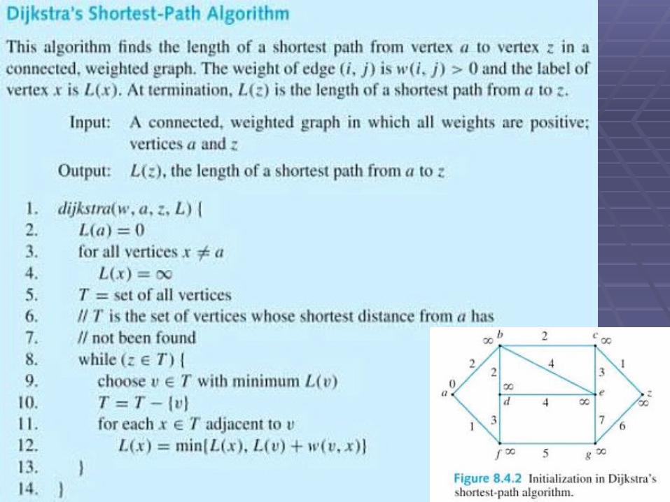
Dijkstra’s Shortest Path AlgorithmDijkstra’s Shortest Path Algorithm
Dijkstra’s algorithm (BFS) for finding the Dijkstra’s algorithm (BFS) for finding the shortest from shortest from aa to to vv, involves assigning , involves assigning labels to vertices. Let labels to vertices. Let L(v)L(v) denote the denote the label of vertex label of vertex vv. At any point, some . At any point, some vertices have vertices have temporary labelstemporary labels and the and the rest have rest have permanent labelspermanent labels, these are , these are shown in red in the following slides. We let shown in red in the following slides. We let TT denote the set of vertices having denote the set of vertices having temporary labels.temporary labels.

Dijkstra’s Shortest Path AlgorithmDijkstra’s Shortest Path Algorithm
For all vertices v do L[v] := For all vertices v do L[v] := od; od;
L(b):= 0; F := 0L(b):= 0; F := 0
do c do c T -> T -> let u be the vertex of F min L.let u be the vertex of F min L. F := F – {u}F := F – {u} for each v adjacent to u for each v adjacent to u do L[v] := L(v) do L[v] := L(v) (L(u) + w(u,v) od (L(u) + w(u,v) od
Where is an infix minimum operator

a z
b c
d e
2
2
2
4
4
1
3
f g
1
3
5
76
Example Graph G(*)

a z
b c
d e
2
2
2
4
4
1
3
f g
1
3
5
76
Initialized Graph G(*)
0

a z
b c
d e
2
2
2
4
4
1
3
f g
1
3
5
76
After First Iteration Graph G(*)
2
1
LabelsL(b) = min{,0+2} L(f) = min{,0+1}
Chose (v= f ) T as minimum L(v)∊
For each x in T adjacent to v: L(x) = min{Lold(x),L(v)+w(v,x)}

LabelsL(b) = min{,0+2} L(f) = min{,0+1} L(d) = min{,0+1+3} L(g) = min{,0+1+5}
a z
b c
d e
2
2
2
4
4
1
3
f g
1
3
5
76
After Second Iteration Graph G(*)
2
6
4
1
Chose (v= b ) T as minimum L(v)∊
For each x in T adjacent to v: L(x) = min{Lold(x),L(v)+w(v,x)}

LabelsL(b) = min{,0+2} L(f) = min{,0+1} L(d) = min{,0+1+3} L(g) = min{,0+1+5}L(c) = min{,0+2+2} L(d) = min{4,0+2+2} --dif. pathL(e) = min{,0+2+4}
a z
b c
d e
2
2
2
4
4
1
3
f g
1
3
5
76
After Third Iteration(*)
42
6
64
1
Chose (v= c ) T as minimum L(v)∊
For each x in T adjacent to v: L(x) = min{Lold(x),L(v)+w(v,x)}

LabelsL(b) = min{,0+2} L(f) = min{,0+1} L(d) = min{,0+1+3} L(g) = min{,0+1+5}L(c) = min{,0+2+2} L(d) = min{4,0+2+2} dif. PathL(e) = min{,0+2+4} L(e) = min{6,0+2+2+3} dif. PathL(z) = min{,0+2+2+1}
a z
b c
d e
2
2
2
4
4
1
3
f g
1
3
5
76
Fourth Iteration(*)
5
42
6
64
1
Chose (v= d ) T as minimum L(v)∊
For each x in T adjacent to v: L(x) = min{Lold(x),L(v)+w(v,x)}

LabelsL(b) = min{,0+2} L(f) = min{,0+1} L(d) = min{,0+1+3} L(g) = min{,0+1+5}L(c) = min{,0+2+2} L(d) = min{4,0+2+2} dif. PathL(e) = min{,0+2+4} L(e) = min{6,0+2+2+3} dif. PathL(z) = min{,0+2+2+1} L(e) = min{6,0+2+2+4} b,f already min
a z
b c
d e
2
2
2
4
4
1
3
f g
1
3
5
76
Fourth Iteration(*)
5
42
6
64
1
Chose (v= z ) T as minimum L(v)∊
For each x in T adjacent to v: L(x) = min{Lold(x),L(v)+w(v,x)}

LabelsL(b) = min{,0+2} L(f) = min{,0+1} L(d) = min{,0+1+3} L(g) = min{,0+1+5}L(c) = min{,0+2+2} L(d) = min{4,0+2+2} dif. PathL(e) = min{,0+2+4} L(e) = min{6,0+2+2+3} dif. PathL(z) = min{,0+2+2+1} L(e) = min{6,0+2+2+4} b,f already min
a z
b c
d e
2
2
2
4
4
1
3
f g
1
3
5
76
Fourth Iteration(*)
5
42
6
64
1
Terminate zT
For each x in T adjacent to v: L(x) = min{Lold(x),L(v)+w(v,x)}

UML For Dijkstra’s Shortest PathUML For Dijkstra’s Shortest Path
See
http://www.comp.dit.ie/pbrowne/Spatial%20Databases%20SDEV4005/DijkstraJava.htm

a z
b c
0
2
2
1
1
2
3
d e
1
Another Graph: Init
Choose v ∊ T with minimum L(v)

a z
b c
0
2
2
1
1
2
3
d e
1
Another Example: 1
LabelsL(b) = min{,0+2} L(d) = min{,0+1}
a.2
a,1
Chose (v= d ) T as minimum L(v)∊

a z
b c
0
2
2
1
1
2
3
d e
1
Another Example: 2
LabelsL(b) = min{,0+2} L(d) = min{,0+1} L(e)=min{,0+1+1} d.2
a,2
a.1
Chose (v= b ) T as minimum L(v)∊
Could have picked e, path to both is 4.

a z
b c
0
2
2
1
1
2
3
d e
1
Another Example: 3
LabelsL(b) = min{,0+2} L(d) = min{,0+1} L(e)=min{,0+1+1} L(c)=min{,0+2+3} L(e)=min{,0+2+1} diff path
d.2
a,2
a.1
b,5
Chose (v= e) T as minimum L(v)∊

a z
b c
0
2
2
1
1
2
3
d e
1
Another Example: 4
d.2
a,2
e,4
a.1
b,5
LabelsL(b) = min{,0+2} L(d) = min{,0+1} L(e)=min{,0+1+1} L(c)=min{,0+2+3} L(e)=min{,0+2+1} diff pathL(z)=min{,0+1+1+2}
Chose (v=z) T as minimum L(v)∊

a z
b c
0
2
2
1
1
2
3
d e
1
Another Example: 4
d.2
a,2
e,4
a.1
b,5
LabelsL(b) = min{,0+2} L(d) = min{,0+1} L(e)=min{,0+1+1} L(c)=min{,0+2+3} L(e)=min{,0+2+1} diff pathL(z)=min{,0+1+1+2}L(c)=min{5,0+1+1+2+2} diff path Terminate zT

128
10
15
n6
14
13
19
19
11n4
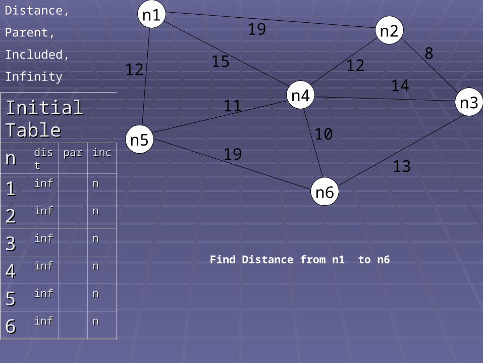
Initial TableInitial Table
nn distdist parpar incinc
11 infinf nn
22 infinf nn
33 infinf nn
44 infinf nn
55 infinf nn
66 infinf nn
Find Distance from n1 to n6
n5
n3
n2n1
12
Distance,
Parent,
Included,
Infinity
128
10
15
n6
14
13
19
19
11n4
Initial TableInitial Table
nn distdist parpar incinc
11 infinf nn
22 infinf nn
33 infinf nn
44 infinf nn
55 infinf nn
66 infinf nn
Find Distance from n1 to n6
n5
n3
n2n1
12
Distance,
Parent,
Included,
Infinity

128
10
15
n6
14
13
19
19
11n4
After iter 1After iter 1
nn distdist parpar incinc
11 00 nonenone yy
22 1919 11 nn
33 infinf nn
44 1515 11 nn
55 1212 11 nn
66 infinf nn
n5
n3
n2n1
12
Distance,
Parent,
Included,
Infinity
Find Distance from n1 to n6

128
10
15
n6
14
13
19
19
11n4
After iter 2After iter 2
nn distdist parpar incinc
11 00 nonenone yy
22 1919 11 nn
33 infinf nn
44 1515 11 nn
55 1212 11 yy
66 3131 55 nn
n5
n3
n2n1
12
Distance,
Parent,
Included,
Infinity
Find Distance from n1 to n6

128
10
15
n6
14
13
19
19
11n4
After iter 3After iter 3
nn distdist parpar incinc
11 00 nonenone yy
22 1919 11 nn
33 2929 44 nn
44 1515 11 yy
55 1212 11 yy
66 2525 44 nn
n5
n3
n2n1
12
New shorter distance
Distance,
Parent,
Included,
Infinity
Find Distance from n1 to n6

128
10
15
n6
14
13
19
19
11n4
After iter 4After iter 4
nn distdist parpar incinc
11 00 nonenone yy
22 1919 11 yy
33 2727 44 nn
44 1515 11 yy
55 1212 11 yy
66 2525 44 nn
n5
n3
n2n1
12
New shorter distance
Distance,
Parent,
Included,
Infinity
Find Distance from n1 to n6

128
10
15
n6
14
13
19
19
11n4
After iter 5After iter 5
nn distdist parpar incinc
11 00 nonenone yy
22 1919 11 yy
33 2727 44 nn
44 1515 11 yy
55 1212 11 yy
66 2525 44 yy
n5
n3
n2n1
12
Distance,
Parent,
Included,
Infinity
Find Distance from n1 to n6

128
10
15
n6
14
13
19
19
11n4
After iter 5After iter 5
nn distdist parpar incinc
11 00 nonenone yy
22 1919 11 yy
33 2727 44 nn
44 1515 11 yy
55 1212 11 yy
66 2525 44 yy
n5
n3
n2n1
12
Distance,
Parent,
Included,
Infinity
Find Distance from n1 to n6
The shortest path from n1 to n4 is 15,
The shortest path from n1 to n6 (via n4) is 15+10=25,

Yet another example Yet another example
Find the shortest path from a to f in the graph G

Yet another example Yet another example
Find the shortest path from a to f in the graph G
Each node is labelled with total
distance and predecessor node

Issues when implementing networks Issues when implementing networks and route finding in GIS(*)and route finding in GIS(*)
Real world networks (e.g. roads) tend to have many Real world networks (e.g. roads) tend to have many
intermediate non-branching vertices (e.g. polylines) intermediate non-branching vertices (e.g. polylines)
which contribute to large adjacency matrices. which contribute to large adjacency matrices.
Networks often multi leveled (e.g walk, bus , train, bus, Networks often multi leveled (e.g walk, bus , train, bus,
ferry, car).ferry, car).
In some cases shortest path problems are subject to In some cases shortest path problems are subject to
additional ‘thematic’ or ‘semantic’ constraints. (e.g. additional ‘thematic’ or ‘semantic’ constraints. (e.g.
road type or quality of transmission line) Constrained road type or quality of transmission line) Constrained
Shortest Path Problem (CSPP).Shortest Path Problem (CSPP).

Issues when implementing networks Issues when implementing networks and route finding in GIS(*)and route finding in GIS(*)
Basic Dijkstra-type algorithms provide Basic Dijkstra-type algorithms provide inconsistent run-times on real-world networks, inconsistent run-times on real-world networks, principally because such networks have very principally because such networks have very limited vertex connectivity (their adjacency limited vertex connectivity (their adjacency matrices are very sparse)matrices are very sparse)11. .
Most network algorithms are 2-D, route on map Most network algorithms are 2-D, route on map maybe be in 3-D, (e.g. cross mountains).maybe be in 3-D, (e.g. cross mountains).

Issues when implementing networks Issues when implementing networks and route finding in GIS(*)and route finding in GIS(*)
The OGC Simple Feature (SFSQL) standard used in The OGC Simple Feature (SFSQL) standard used in PostGIS does not include any network representation, PostGIS does not include any network representation, therefore an additional Network ADT must be provided, therefore an additional Network ADT must be provided, which must integrate with the existing standard. Ideally which must integrate with the existing standard. Ideally we would want to avoid two distinct non-compatible we would want to avoid two distinct non-compatible ADTs. The existing OGC data structures and algorithms ADTs. The existing OGC data structures and algorithms for 2-dimensional objects contain polygons, edges, and for 2-dimensional objects contain polygons, edges, and vertices and must be augmented with connectivity vertices and must be augmented with connectivity information. Also, the OGC SFSQL must integrate with information. Also, the OGC SFSQL must integrate with the 1-D route finding algorithms and network data the 1-D route finding algorithms and network data structures. GML provides network support. structures. GML provides network support.

Issues when Issues when usingusing networks and networks and route finding in GIS(*)route finding in GIS(*)
The user must be able to understand how The user must be able to understand how to use the Network ADT (e.g. pgRouting).to use the Network ADT (e.g. pgRouting).
User must insure that the data in the User must insure that the data in the appropriate format for the network ADT. appropriate format for the network ADT. This may require manual or software This may require manual or software conversion of the data.conversion of the data.

pgRouting: preperationpgRouting: preperation A simple line graph needs to be transformed to include network A simple line graph needs to be transformed to include network
topology, with connective nodes and edges, by issuing this topology, with connective nodes and edges, by issuing this command in the SQL Shell or pgAdmin SQL Query tool:command in the SQL Shell or pgAdmin SQL Query tool:
SELECT assign_vertex_id('edges', 0.001, 'the_geom', 'gid');SELECT assign_vertex_id('edges', 0.001, 'the_geom', 'gid');
assign_vertex_id()assign_vertex_id() is a function included with the pgRouting extension. is a function included with the pgRouting extension. This is explained in the tutorial.This is explained in the tutorial.
In general, we need to update a table by adding a numerical value In general, we need to update a table by adding a numerical value to a column that we previously created when issued the to a column that we previously created when issued the CREATE TABLECREATE TABLE statement.statement.
UPDATE edges SET length = length(the_geom);UPDATE edges SET length = length(the_geom);
This creates a length field to hold the length value of network This creates a length field to hold the length value of network edges. This can be a cost. We would also use the same statement edges. This can be a cost. We would also use the same statement to update a “cost” column.to update a “cost” column.

pgRoutingpgRouting
Now we can use any of the GIS functions Now we can use any of the GIS functions provided by PostGIS and pgRouting.provided by PostGIS and pgRouting.
Dijkstra’s algorithm is a good single-Dijkstra’s algorithm is a good single-source routing algorithm provided by source routing algorithm provided by pgRouting.pgRouting.

Methods for AnalysisMethods for Analysis
To run the query and get an answer in To run the query and get an answer in WKT (Well-Known-Text), you can issue WKT (Well-Known-Text), you can issue this command in pgAdmin’s SQL Query this command in pgAdmin’s SQL Query tool:tool:
SELECT gid, AsText(the_geom) AS the_geomSELECT gid, AsText(the_geom) AS the_geom
FROM dijkstra_sp('edges', 1, 8);FROM dijkstra_sp('edges', 1, 8);
Starting node = 1Starting node = 1
Destination node = 8Destination node = 8
‘‘edges’ = the table containing the network edges’ = the table containing the network

ResultsResults Dijkstra’s results expressed in WKT:Dijkstra’s results expressed in WKT:
The “gid” is synonymous with “FID” in ArcGIS, and “the_geom” in The “gid” is synonymous with “FID” in ArcGIS, and “the_geom” in this case is expressed in WKT. The numbers shown represent this case is expressed in WKT. The numbers shown represent coordinate pairs that make up points along a polyline.coordinate pairs that make up points along a polyline.
WKT is an OGC (Open Geospatial Consortium) standard.WKT is an OGC (Open Geospatial Consortium) standard. In order to view the result in OpenJump we usually include the In order to view the result in OpenJump we usually include the
additional steps of making a result table or using an SQL view. additional steps of making a result table or using an SQL view. Details are in the labs.Details are in the labs.

Dijkstra, A*, Shooting*Dijkstra, A*, Shooting*
Anton Patrushev (Orkney, Inc.)

Dijkstra, A*, Shooting*Dijkstra, A*, Shooting*
Anton Patrushev (Orkney, Inc.)

Dijkstra, A*, Shooting*Dijkstra, A*, Shooting*
Anton Patrushev (Orkney, Inc.)
A heuristic algorithmA heuristic algorithm
A heuristic algorithm is an algorithm that is A heuristic algorithm is an algorithm that is able to produce an acceptable solution to able to produce an acceptable solution to a problem in many practical scenarios, but a problem in many practical scenarios, but for which there is no formal proof of its for which there is no formal proof of its correctness. The algorithm uses a “correctness. The algorithm uses a “rule of rule of thumbthumb” or “” or “educated guesseducated guess” ” to help find a to help find a solution. solution.

A-Star a heuristic algorithmA-Star a heuristic algorithm
A* takes uses the A* takes uses the distance so far plus cost distance so far plus cost heuristicheuristic. .
Two distinctions between Dijkstra and A*.Two distinctions between Dijkstra and A*. A* uses a heuristic e.g. A* uses a heuristic e.g. remaining distanceremaining distance.. A* uses the A* uses the distance already traveleddistance already traveled and not and not
simply the local cost from the previously simply the local cost from the previously expanded node. This in contrast to Dijkstra expanded node. This in contrast to Dijkstra which is a greedy algorithm. Dijkstra can be which is a greedy algorithm. Dijkstra can be used when the estimate to the goal is difficult used when the estimate to the goal is difficult or impossible to calculate.or impossible to calculate.

A-Star a heuristic algorithmA-Star a heuristic algorithm
A* takes the distance already traveled into A* takes the distance already traveled into account and not simply the local cost from account and not simply the local cost from the previously expanded node. For each the previously expanded node. For each node x traversed, it maintains 3 values:node x traversed, it maintains 3 values: g(x)g(x) : the actual shortest distance traveled : the actual shortest distance traveled
from initial node to current node from initial node to current node xx.. h(x)h(x) : the estimated (or "heuristic") distance : the estimated (or "heuristic") distance
from current node to goalfrom current node to goal f(x)f(x) : the sum of : the sum of g(x)g(x) and and h(x).h(x).

A-Star a heuristic algorithmA-Star a heuristic algorithm
The heuristics The heuristics h(x)h(x) must not be an must not be an overestimate of the distance to the goal. overestimate of the distance to the goal. The Euclidean (or straight line) distance is The Euclidean (or straight line) distance is always less than or equal to the road always less than or equal to the road distance.distance.

pgRouting data structurepgRouting data structure
For further details of the data pgRouting structures seehttp://pgrouting.postlbs.org/wiki/WorkshopFOSS4G2007
http://pgrouting.postlbs.org/wiki

A line graph for edge A line graph for edge representationrepresentation

Computational complexityComputational complexity11
Computational complexity theory deals Computational complexity theory deals with the costs of computing a solution with the costs of computing a solution given problem. Costs can be measured in given problem. Costs can be measured in terms of time (e.g. number of iterations), terms of time (e.g. number of iterations), space( e.g. memory required), best, space( e.g. memory required), best, average and worst cases. average and worst cases.
CC can be applied to a wide range of CC can be applied to a wide range of algorithms including shortest path (e.g. algorithms including shortest path (e.g. Dijkstra and A*). Dijkstra and A*).

Complexity ofComplexity of Dijkstra DijkstraMathWorld--A Wolfram Web ResourceMathWorld--A Wolfram Web Resource
The worst-case running time for the Dijkstra The worst-case running time for the Dijkstra algorithm on a graph with algorithm on a graph with nn nodes and nodes and mm edges edges is is O(nO(n22)) because it allows for directed cycles. It because it allows for directed cycles. It even finds the shortest paths from a source even finds the shortest paths from a source node node ss to all other nodes in the graph. This is to all other nodes in the graph. This is basically basically O(nO(n22)) for node selection and for node selection and O(m)O(m) for for distance updates. While distance updates. While O(nO(n22)) is the best is the best possible complexity for dense graphs, the possible complexity for dense graphs, the complexity can be improved significantly for complexity can be improved significantly for sparse graphs. sparse graphs.

Complexity ofComplexity of A* A*WikipediaWikipedia
The The timetime complexity of A* depends on the heuristic. In complexity of A* depends on the heuristic. In the worst case, the number of nodes expanded is the worst case, the number of nodes expanded is exponentialexponential in the length of the solution (the shortest in the length of the solution (the shortest path), but it is path), but it is polynomialpolynomial when the search space is a when the search space is a tree, there is a single goal state, and the heuristic tree, there is a single goal state, and the heuristic function h meets the following condition:function h meets the following condition:
| h(x) − h*(x) | = O(log h*(x)) | h(x) − h*(x) | = O(log h*(x)) where h* is the optimal heuristic, i.e. the exact cost to get where h* is the optimal heuristic, i.e. the exact cost to get
from x to the goal. The error of h should not grow faster from x to the goal. The error of h should not grow faster than the logarithm of the “perfect heuristic” h* that than the logarithm of the “perfect heuristic” h* that returns the true distance from x to the goalreturns the true distance from x to the goal

OpenGIS Location Services (OpenLS): Core Services
Please read:
OpenGIS Location Services (OpenLS): Core Services

OGC OpenLSOGC OpenLS Standards with respect to LBSs have been set up by the
International Standard Organisation (ISO) and by the Open Geospatial Consortium (OGC). The OGS has released the Open Location Services (OpenLS - Open Geospatial Consortium 2005). OpenLS defines core services, their access and abstract data types which form together a framework for a open service platform, the so called GeoMobility server. The server acts as application server and should process and answer core service requests. The role of this server is pictured in the previous slide. It should be noticed that service requests to a GeoMobility server can be send from a mobile user, from Internet users and also from other application servers.

Applications of LBSApplications of LBS Traffic Information: there is a traffic queue, so turn right.Traffic Information: there is a traffic queue, so turn right. Emergency Services: help, I'm having a heart attack!Emergency Services: help, I'm having a heart attack! Roadside Emergency; “help, my car has broken down!Roadside Emergency; “help, my car has broken down! Law Enforcement: what is the speed limit on this roadLaw Enforcement: what is the speed limit on this road Classified Advertising; where are nearby sales featuring antiquesClassified Advertising; where are nearby sales featuring antiques Object visualization: where is the historic parcel boundaryObject visualization: where is the historic parcel boundary Underground Object Visualization: “where is the water main?”Underground Object Visualization: “where is the water main?” Public Safety Vehicle Mgt: who is closest to that emergency?”Public Safety Vehicle Mgt: who is closest to that emergency?” Location-Based Billing; free calls on your phone, in a locationLocation-Based Billing; free calls on your phone, in a location Leisure Information: How do we get to the Club from hereLeisure Information: How do we get to the Club from here Road Service Information: Where is the nearest petrol stationRoad Service Information: Where is the nearest petrol station Directions: I'm lost, where is nearest Metro stationDirections: I'm lost, where is nearest Metro station Vehicle Navigation; how do I get back to the Interstate from here?Vehicle Navigation; how do I get back to the Interstate from here? Vehicle Theft Detection: my car has been stolen, where is itVehicle Theft Detection: my car has been stolen, where is it Child Safety: tell me if my child strays beyond the neighborhood.Child Safety: tell me if my child strays beyond the neighborhood.

Location Based ServicesLocation Based Services
Please read Navigation Systems: A Spatial Database Perspective
http://www-users.cs.umn.edu/~shekhar/research/lbsChapter.pdf

OGS OpenLSOGS OpenLS
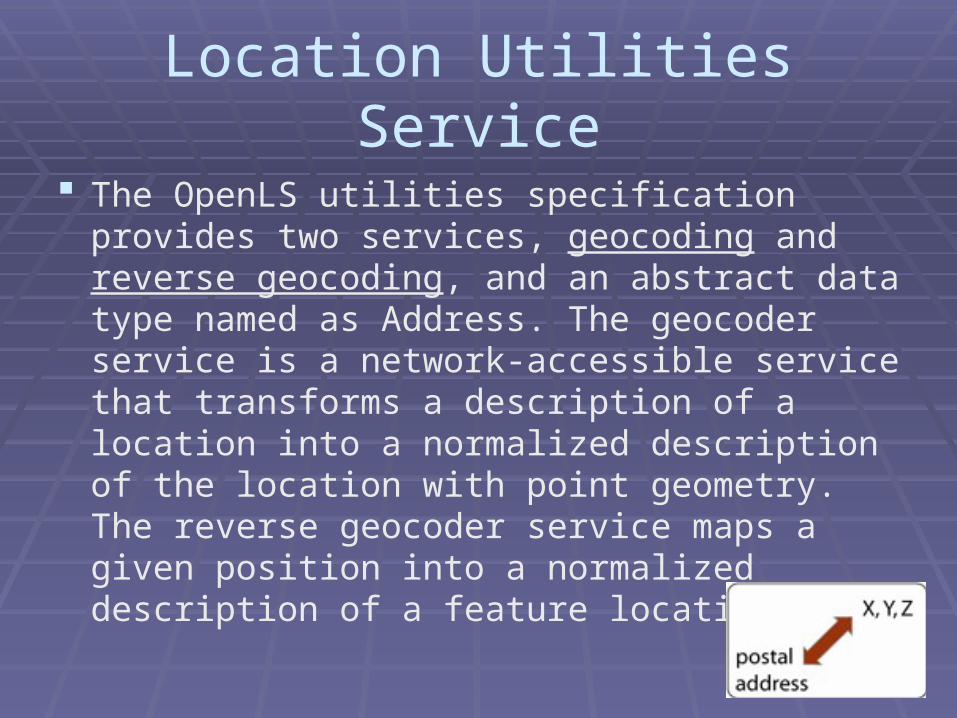
Location Utilities Service
The OpenLS utilities specification provides two services, geocoding and reverse geocoding, and an abstract data type named as Address. The geocoder service is a network-accessible service that transforms a description of a location into a normalized description of the location with point geometry. The reverse geocoder service maps a given position into a normalized description of a feature location.

Directory Service
The directory service provides a search capability for one or more points of interest (e.g., a place, product, or service with a fixed position) or area of interest (e.g., a polygon or a bounding box). The DS is a network-accessible service that provides access to an online directory (a kind of spatial Yellow Pages) to find the location of a specific or nearest place, product or service. An example query is ‘‘Where is the nearest thesis binder to Kevin Street?’’

Presentation Service. This service deals with visualization of the
spatial information as a map, route, and/or textual information (e.g., route description). The Presentation (Map Portrayal) Service portrays a map made up of a base map derived from any geospatial data and a set of Abstract Data Types as overlays.

Gateway Service This service enables obtaining the position of a
mobile terminal from the network. The Gateway Service is a network-accessible service that fetches the position of a known mobile terminal from the network. The gateway is the interface between the GeoMobility Server and the Location Server from the Positioning Service. It is useful to request for the current location with different modes (e.g. multi or single terminal, immediate or periodic position).

Gateway Service Details
GMLC/MPC: this interface is modeled after the Mobile Location Protocol (MLP),
Standard Location Immediate Service.
Gateway Mobile Location Center
Position Determination
Entity

Route Determination Service
This service provides the ability to find a best route between two points that satisfies user constraints. RDS determines travel routes and navigation information according to diverse criteria.

Suggested reading Suggested reading PaperPaper
Navigation Systems: A Spatial Database Perspective by Shashi Navigation Systems: A Spatial Database Perspective by Shashi Shekhar, Ranga Raju Vatsavai, Xiaobin Ma, and Jin Soung Shekhar, Ranga Raju Vatsavai, Xiaobin Ma, and Jin Soung
Yoo.Yoo. http://www-users.cs.umn.edu/~shekhar/research/lbsChapter.pdfhttp://www-users.cs.umn.edu/~shekhar/research/lbsChapter.pdf
BookBook: Location-Based Services: by Schiller & Voisard: Location-Based Services: by Schiller & Voisard WebWeb http://http://www.opengeospatial.org/standards/olswww.opengeospatial.org/standards/ols http://pgrouting.postlbs.org/http://pgrouting.postlbs.org/ http://http://www.openrouteservice.orgwww.openrouteservice.org// http://www.davidgis.fr/documentation/pgrouting-1.02/http://www.davidgis.fr/documentation/pgrouting-1.02/
http://www.utdallas.edu/~ama054000/rt_tutorial.htmlhttp://www.utdallas.edu/~ama054000/rt_tutorial.html http://www.directionsmag.com/article.php?article_id=2876&trv=1http://www.directionsmag.com/article.php?article_id=2876&trv=1 http://www.geographie.uni-bonn.de/karto/http://www.geographie.uni-bonn.de/karto/