outdoor scene segmentation and object classification the appearance based information from the...

Outdoor scene segmentation and object classification

Using cluster based perceptual Organization

Neha Dabhi#1 Prof.HirenMewada

*2

P.G. Student,VTP Electronics & communication Dept.,

Chaotar Instiute of Science & Technology, Changa,Anand, India

[email protected]

Associate Professor,VTP Electronics & communication Dept.,

Chaotar Instiute of Science & Technology, Changa,Anand, India

[email protected]

ABSTRACT:

Humans may be using high-level image understanding and object recognition skills to produce more meaningful

segmentation while most computer applications depend on image segmentation and boundary detection to achieve some

image understanding or object recognition. The high level and low level image segmentation model may generate

multiple segments for the single object within an image. Thus, some special segmentation technique is required which

is capable to group multiple segments and to generate single objects and gives the performance close to human visual

system. Therefore, this paper proposes the perceptual organization model to perform the above task. This paper

addresses the outdoor scene segmentation and object classification using cluster based perceptual organization.

Perceptual organization is the basic capability of the human visual system is to derive relevant grouping and structures

from an image without prior knowledge of its contents . Here, Gestalt laws (Symmetry, alignment and attachment) are

utilized to find the relationship between patches of an object obtained using K-means algorithm. The model mainly

concentrated on the connectedness and cohesive strength based grouping. The cohesive strength represents the non-

accidental structural relationship of the constituent parts of a structured part of an object. The cluster based patches are

classified using boosting technique. Then the perceptual organization based model is applied for further classification.

The experimental result shows that, it works well with the structurally challenging objects, which usually consist of

multiple constituent part and also gives the performance close to human vision.

1.Introduction:

Image segmentation is considered to be one of the fundamental problems for computer vision[Gonzalvez&Woods]. A

primary goal of image segmentation is to partition or division of an image into regions which has coherent properties so

that each region corresponds to an object or area of interest [Shah,2008]. The outdoor scenes can be divided into two

categories, namely, unstructured objects (e.g., skies, roads, trees, grass, etc.) and structured objects (e.g., cars, buildings,

people, etc.). Unstructured objects usually comprise the backgrounds of images. The background objects usually have

nearly homogenous surfaces and are distinct from the structured objects in images. Many recent appearances-based

Neha Dabhi et al , International Journal of Computer Science & Communication Networks,Vol 3(4),240-264

240

ISSN:2249-5789

mailto:[email protected]

mailto:[email protected]

methods have achieved high accuracy in recognizing these background object classes or unstructured objects in the

scene [Shotton,2009], [Winn et al.,2005], [Gould et al.,2008].

There are two challenges for outdoor scene segmentation: 1) Structured objects that are often composed of multiple

parts, with each part having distinct surface characteristics (e.g., colors, textures, etc.). Without certain knowledge about

an object, it is difficult to group these parts together. 2) The Background objects have various shape and size. To

overcome these challenges some object specific model is required. In this, our research objective is to detect object

boundaries in outdoor scene images solely based on some general properties of the real world objects such as

―perceptual organization laws‖.

Fig 1.1: Block diagram of outdoor scene segmentation

The fig 1.1 shows the basic block diagram of outdoor scene segmentation. It consist image textonization module for

recognizing the appearance based information from the scene,Feature selection module for extraction of features for

training the classifier, Boosting for classifying the objects from the scene and finally Perceptual Organization Model for

merging multiple segmentation of the particular object.

2.Related Work:

Perceptual Organization can be defined within the context of Visual Computing as the particular approach in

qualitatively and or quantitatively characterizing some visual aspect of a scene through computational methodologies

inspired by Gestalt psychology. This approach has found special attention in imaging related problems due to its ability

to support humanly meaningful information even in the presence of incomplete and noisy contexts. This special track

aims to offer an opportunity for new ideas and applications developed on perceptual organization to be brought to the

attention of in the wider Computer Science community. It is difficult to perform object detection, recognition, or proper

assessment of object-based properties (e.g., size and shape) without a perceptually coherent grouping of the ―raw‖

regions produced by image segmentation. Automatic segmentation is far from being perfect. First, human segmentation

actually involves performing object recognition first based on recorded models of familiar objects in the mind. Second,

color and lighting variations causes tremendous problems as it create highly variable appearances of objects.for

automatic algorithms[Xuming He&Zemel,2006] but are effectively discounted by humans (again because of the

models); different segmentation algorithms differ in strengths and weaknesses because of their individual design

principlesTherefore, some form of regularization is needed to refine the segmentation [Luo&Guo,2003]. Regularization

may come from spatial color smoothness constraints (e.g., MRF—Markov random field), contour/shape smoothness

constraints (e.g., MDL—minimum description length), or object model constraints. To this end, perceptual grouping is

Input

Image

Image

textonization

Feature

selection

module

Boosting Perceptual

organization

model

Resultant

Segmented

Image


241

ISSN:2249-5789

expected to all in the so-called ―semantic gap‖ and play a significant role in bridging image segmentation and high-level

image understanding. Perceptual region grouping can be categorized as non-purposive and purposive.

The organization of vision is divided into: 1)low level vision :which consist finding edges ,colors and location of object

in space,2)mid level vision: which consist determing object features and segregate object from the background,3)High

level vision : which consist recognition of object,scene and face.Thus there are three cues for perceptual grouping which

are low level ,mid level and high level cues.

Low-Level cue contain brightness, color, texture, depth, motion based grouping.Martin et al proposed one method

which learns and detects natural image boundaries using local brightness, color, and texture cues. The two main results

are:1) that cue combination can be performed adequately with a simple linear model and 2) that a proper, explicit

treatment of texture is required to detect boundaries in natural images. [Martin et al, 2004]. Sharma & Davis presented a

unified method for simultaneously acquiring both the location and the silhouette shape of people in outdoor scenes. The

proposed algorithm integrates top-down and bottom-up processes in a balanced manner, employing both appearance

and motion cues at different perceptual levels. Without requiring manually segmented training data, the algorithm

employs a simple top-down procedure to capture the high-level cue of object familiarity. Motivated by regularities in

the shape and motion characteristics of humans, interactions among low-level contour features are exploited to extract

mid-level perceptual cues such as smooth continuation, common fate, and closure. A Markov random field formulation

is presented that effectively combines the various cues from the top-down and bottom-up processes. The algorithm is

extensively evaluated on static and moving pedestrian datasets for both detection and segmentation.[ Sharma &

Davis ,2007]

Mid-Level cue contain Gestalt law based segmentation.It contains continuity, closure, convexity, symmetry, parallism

etc. Kootstra and D. Kragic developed system for object detection, object segmentation, and segment evaluation of

unknown objects based on Gestalt principles. Firstly, the object-detection method will generate hypotheses (fixation

points) about the location of objects using the principle of symmetry. Next, the segmentation method separates

foreground from background based on a fixation point using the principles of proximity and similarity. The different

fixation points and possibly different settings for the segmentation method result in a number of object-segment

hypotheses. Finally, the segment-evaluation method selects the best segment by determining the goodness of each

segment based on a number of Gestalt principles for figural goodness [Kootstra et al,2010].

High-Level cue contain familiar objects and configurations which is still in process.High level information –derived

attributes,shading,surfaces,occlusion,recognition etc.

Thus,low level cues requires the guidance of high level cues to overcome noice ; while high level cues relies on low

level cues to reduce the computational complexity.Here, in the proposed work color and texture are used to find the

connectness between patches and according the whole object can be merged together.In this for finding the relation


242

ISSN:2249-5789

between the patches the geometric statical knowledge based laws are utilized.Here recognition is also utilized at the

third stage in the boosting of the desired object.So,it utilizes all three cues for better performance.

3.IMAGE SEGMENTATION ALGORITHM:

Start

Receive an image training Set

Conversion of RGB image to CIELab

Color space

Image textonization module

Select Texture Layout features from the

text on images

Learn Gentleboost model based on selected

textured layout Features

Evaluate the

Performance of

classifier for desired

Clustered Object.

Achieved?

Perceptual Organization based

segmentation

Segmented Output

Fig 3.1:Flow Diagram of Proposed Image Segmentation algorithm

Yes No


243

ISSN:2249-5789

Here, we present an image segmentation algorithm based on POM for outdoor scenes.The objective of this research

paper is to explore detecting object boundaries which are based on some general properties of the real-world objects,

such as perceptual organization laws, which is independent of the prior knowledge of the object. The POM

quantitatively incorporates a list of mid level -Gestalt cues. The proposed image segmentation algorithm for an outdoor

scene is as shown in fig 2. Now we will see the flow diagram of whole process in fig 3.1.

3.1 Conversion of the image into CIE lab color space

The first step is convert the training images into the perceptually uniform CIE Lab color space.The CIE Lab is specially

designed to best approximate for uniform color spaces. We utilized CIE color space for three color bands because the

CIE Lab color space is partially invariant to scene lighting modifications—only the L dimension changes in contrast to

the three dimensions of the RGB color space, for instance. The nonlinear relations for L * , a *, and b * are intended to

mimic the nonlinear response of the eye. Furthermore, uniform changes of components in the L * a *b * color space aim

to correspond to uniform changes in perceived color, so the relative perceptual differences between any two colors in L*

a *b * can be approximated by treating each color as a point in a three-dimensional space (with three components: L * ,

a *, b *) and taking the Euclidean distance between them.In this the perceived color difference should correspond to

Euclidean distance in the color space chosen to represent features[Kang et. Al., 2008]. Thus, the CIE lab utilized for the

best approximation of the perceptual visualization.

3.2 Image Textonization

Natural scenes are rich in color and texture and the human visual system exhibit remarkable ability to detect subtle

differences in texture that is generated from an aggregate of fundamental microstructure of an element. The key to this

method is to use textons. The term ―Texton‖ is conceptually proposed by Julesz.[Julesz,1981].It is a very useful concept

in object recognition.It is the compact representations for the range of different appearances of an object. For this we

utilize textons [Leung, 2001] which have been proven effective in categorizing materials [Varma, 2005] as well as a

generic object classes and context. The term textonization first presented by[Malik,2001] for describing human textural

Image Augmentation

Image Convolution

Fig 3.2:Image

textonization Module

Image Clustering

Image Textonization Module


244

ISSN:2249-5789

perception. A texton images generated from an input image is an image of pixels , where each pixel value in the texton

image is a representation of its corresponding pixel value in the input image. Specifically, each pixel value of the input

image is replaced by a representation e.g., cluster identification, corresponding to the pixel value of the input image

after the input image is being processed. For example, an input image is convolved with a filter bank resulting in 17

degree vectors for each pixel of the input images. The image textonization mainly has two modules: Image Convolution

and Image Clustering. And before clustering the augmentation is carried out to improve the accuracy. The whole image

textonization module is as shown in Fig 3.2.

The advantages of textons are:

1. Effective in categorizing materials

2. Find generic object classes.

Image textonization process includes the image convolution module and image clustering module which is discussed as

below:

3.2.1 Image convolution:

Image convolution process includes the convolution of the pre-processed image training set with a filter bank. There are

many types of filter banks like MR8 filter bank ,28D filter Bank, Lung and Malik set etc. [Kang et. Al., 2008]In that

MR8 filter bank is utilized in the monochrome image for texture classification experiments. It cannot be applied to color

images. The 17 D filter bank is designed for color image segmentation .So MR8 filter bank is expanded up to the

infrared band image.The convolution module uses a seventeen dimensional filter bank consisting of Gaussians at scales

1, 2 and 4 . A derivative of Gaussian along x and y axes at scales 2 and 4 and finally Laplacian of Gaussian at scales

1,2,4 and 8.Here the image is first converted from RGB image into the CIE Lab color space. Thus, these Gaussian filters

are computed on all three channels of CIE Lab color space and the rest of the filters are only applied to the luminous

channel.

3.2.2 Image Augmentation

The output resulted from convolution is augmented with CIE lab color space. It slightly increases the efficiency.

3.2.3 Image Clustering:

Before clustering the output of convolution which is 17 Dimensional vectors is augmented with the CIE Lab image,

thus finally the 20 Dimensional vectors are resulted. The resulted vector is then clustered using the k-means clustering

method. In this the number of clusters K must be specified previously. In that from the color image the identification of

number of cluster also can be possible. The k-means clustering is preferred because it a consider pixels with relatively

close intensity values as belonging to one segment even if they are not locationally close and also it is not complex.

3.2.3.1 K-means clustering

K-Means algorithm is an unsupervised clustering algorithm that classifies the input data points into multiple classes

based on their inherent distance from each other. The algorithm assumes that the data features form a vector space and

tries to find natural clustering in them. The points are clustered around centroids kii ...1 which are obtained by

minimizing the objective


245

ISSN:2249-5789

2

1

)( i

k

i sixj

jxV

…(3.1)

where there are k clusters kiSi ,...2,1, and i is the centroid or mean point of all the pointsij sx .

The algorithm takes a two dimensional image as input. Various steps in the algorithm are as follows:

1. Compute the intensity distribution(also called the histogram) of the intensities.

2. Initialize the centroids with k random intensities.

3. Repeat the following steps until the cluster labels of the image does not change

anymore.

4. Cluster the points based on distance of their intensities from the centroid intensities.

2)()( minarg i

ii xc …(3.2)

5. Compute the new centroid i for each of the clusters.

The main advantage of the K-means method is it gives the descritized representation ,such as codebook of features or

texton images and also it can model the whole image or specific region of the image with or without spatial context of

the image. The Fig 3.3 shows the textonization process applied to image in our case it is applied on preprocessed image

and in the preprocessing the image is converted into CIE lab color space.

Fig 3.3 :Textonization Process

3.3 Boosting :

Boosting (also known as arcing — Adaptive Resampling and Combining) is a general method for improving the

performance of any learning algorithm. It is an ensemble method. Certain classification problems where a single

classifier does not perform well as below:

Statistical Reasons

Inadequate availability of data.

Presence of too much data.

Divide and conquer - Data having complex class separations.

Data Fusion.


246

ISSN:2249-5789

Thus, ensembling is used to overcome the above problems and for improvement of the performance. In an ensemble, the

output on any instance is computed by averaging the outputs of several hypotheses, possibly with a different weighting.

Hence, we should choose the individual hypotheses and their weight in such a way as to provide a good fit. This

suggests that instead of constructing the hypotheses independently, we should construct them such that new hypotheses

focus on instances that are problematic for existing hypotheses.

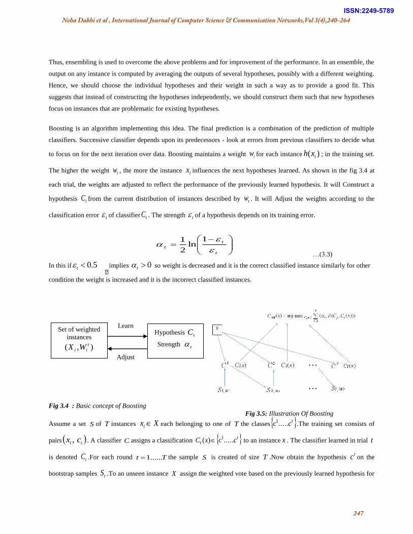
Boosting is an algorithm implementing this idea. The final prediction is a combination of the prediction of multiple

classifiers. Successive classifier depends upon its predecessors - look at errors from previous classifiers to decide what

to focus on for the next iteration over data. Boosting maintains a weight iw for each instance )( ixh ; in the training set.

The higher the weight iw , the more the instance ix influences the next hypotheses learned. As shown in the fig 3.4 at

each trial, the weights are adjusted to reflect the performance of the previously learned hypothesis. It will Construct a

hypothesis tC from the current distribution of instances described by tw . It will Adjust the weights according to the

classification error t of classifier tC . The strength t of a hypothesis depends on its training error.

t

t

t

1ln

2

1

…(3.3)

In this if 5.0t

implies 0t so weight is decreased and it is the correct classified instance similarly for other

condition the weight is increased and it is the incorrect classified instances.

Fig 3.4 : Basic concept of Boosting

Fig 3.5: Illustration Of Boosting

Assume a set S of T instances X xi each belonging to one of T the classes tc......c1.The training set consists of

pairs ii cx , . A classifier C assigns a classification tt cxC ......c)( 1 to an instance x . The classifier learned in trial t

is denoted tC .For each round Tt ......1 the sample S is created of size T .Now obtain the hypothesis tc on the

bootstrap samples tS .To an unseen instance X assign the weighted vote based on the previously learned hypothesis for

Set of weighted

instances

),( t

ii WX

Hypothesis tC

Strength t

Learn

Adjust


247

ISSN:2249-5789

all round T and generated the classifier tC at each round. Now obtain a final hypothesis by aggregating the T

classifiers which are shown in Fig 3.5. Freund & Schapire in 1996 proved that Boosting provides a larger increase in

accuracy than Bagging. Bagging provides a modest improvement more consistent [Freund & Schapire, 1996]. Boosting

is particularly subject to over-fitting when there is significant noise in the training data.

3.4 Perceptual Organization Model:

Let represent a whole image domain that consists of the regions that belong to the backgrounds BR and the regions

that belong to structured objects SR , SB RR . After the object identified by posting, we know ours object that

we want to segment which is called the region SR . Let oP be the initial part of the object which is obtained from the k-

means clustering technique. Let a denote a small patch from the initial partition oP . For )()( So RaPa , a is

one of the constituent parts of an unknown structured object. Based on initial part a ,we want to find the maximum

region aR SR so that the initial part a aR and for any uniform patch i ; where )()( RaiPi o , i should have

some special structural relationships that obey the non-accidents principle with the remaining patches Ra .Here we

have applied Gestalt laws on those and merged based on the cohesive strength and boundary energy function.

3.4.1 Cohessive Strength

It is the ability of the patch to remain connected with the other. It measures how tightly the image patch i is attached to

the other parts of the structured object. The Cohesive Strength is calculated as:

ijijijessCohessiven

For )(ineighborsjai …

(3.4)

Here, a is the initial part and j is the other neighboring patch of the patch i . ij , ij , ij measures the symmetry ,

alignment ,attachment between the two patches. If the initial part a is equal to the image patch i then cohesive strength

is 1.Thus the maximum value of the cohesive strength can be achieved, as it belongs to the structured object.

3.4.1.1 Symmetry

Here, we have measured the symmetry between i and j patches along the vertical direction because the parts which

are approximately symmetric along the vertical axis are very likely belonging to the same object .Symmetry of i and j

along the vertical axis is defined as [Cheng et al., 2012]

ji yyij ,1 … (3.5)

Where is the Kronecker delta Function,

iy , jy are the column coordinates of the centroids of patches i and j.

If iy and jy are very close, this means that the patches are approximately symmetric along the vertical direction.


248

ISSN:2249-5789

3.4.1.2 Alignment

This alignment test encodes the continuity law. The good continuation between components can only be established if

the object parts are strictly aligned along a direction , so the boundary of the merged components will have a good

continuation. The principle of good continuation states that a good segmentation should have smooth boundaries.

Alignment of i and j is defined as

0ij if jijiij

OR

1ij if jijiij

… (3.6)

Where, ij is the common boundary between patches i and j , denotes the empty set.

3.4.1.3 Attachment

If patches i and j are neither symmetric nor aligned then we have to find the attachment. It gives a measure of how

much the image patch i is attached to the other patch j . It is defined as [Cheng et al.,2012]

)()(

))()cos(exp(,

ji

ij

jiLL

L

… (3.7)

It depends on the ratio of the common boundary length between two patches and sum of the boundary length between

two patches. Here, is angle between the line connecting two ends of ij and the horizontal line starting from one end

of ij . )( iL , )( jL is the length of the patch i and j . )( ijL Is the length of the common boundary of the patches

i and j .

When )( iL >> )( jL or )( jL >> )( iL then a larger one belongs to the background object such as wall, road etc.

If the patch i and j have similar sizes and share a long common boundary, this means that and might be adjacent in

the 3-D world. In other words, i is considered to be in close proximity to j . For this case, i and j are considered to be

strongly attached. Here ‗ cos ‘ is used as controlling parameter. Because two patches i and j are tightly attached

along horizontal axis but they may still belong to the neighboring objects. In general, vertically attached parts have

larger attachment strength than those horizontally attached. Thus, it controls the cohesive strength of two attaching

patches according to the attachment orientation.


249

ISSN:2249-5789

(a) (b)

(c) (d)

3.4.2 Energy Boundary Function

The boundary energy function is a good way for measuring how good a region is[Cheng et al.,2012]. Any optimal

segmentation is a merged result of elementary regions. Those elementary regions are equivalent to the UC objects in

perceptual organization. The elementary regions are the fundamental units of the optimal segmentation of the image. In

this the region will be merged based on the Boundary function. That boundary function encodes the local structural

relationship between the neighboring parts of the structured object. That function is designed by using gestalt laws. That

encodes the Symmetry, alignment and attachment into the function and based on the merging will be performed. The

function is defined as [Cheng et al., 2012]

)(),( ai SSabs

eyxf

With ),( yx R … (3.8)

Where, is a weight vector which is empirically set to ]5.3,18[ in our implementation. Vector ],[ iii CBS ,

which is a point in the structural context space encoding the structural information about image patch i , which depends

on the boundary complexity function and the cohesive strength. aS is a reference point in the structure‘s context spaces,

which encodes the structural information of initial part. Since it is the only known information that we have about the

unknown structured object, we use as a reference point. Notice that, at the beginning of the grouping process, region

only contains initial part .In that case 1),(, yxfai , which means that we always set the largest weighted

element to initial part. Then, we try to grow region by including the neighbors of the region based on the cohesive

strength.If the two patches are neighbor and strongly attached with each other then the cohesive strength is higher. iC Is

the cohesive strength which is defined in section 3.3.1.

Then, ),( yxf which is called the boundary function which is designed by four Gestalt laws i.e., Similarity, Symmetry,

Alignment and Attachment are used for designing the boundary energy function, which is defined as:

Fig 3.6 : a) Symmetry relations: the red

dots indicate the centroids of the

components. (b) Alignment relations. (c)

Two components are strongly attached. (d)

Two components are weakly attached.

[Cheng et al.,2012]


250

ISSN:2249-5789

)(

),(

][RL

dxdyyxf

RE R

… (3.9)

Where, )( RL is the boundary length of the region R. ),( yxf Is the weight function in the region R . The criterion of

region goodness depends on how weight function ),( yxf is defined and the boundary length )( RL . Here the

function ),( yxf encodes the local structural relationships between neighboring parts contained in region R. Here the

boundary length )( RL reflects the global property of region R .In this we have find the energy of the reference patch

and the energy of after the union of the two patches if the energy of the union of the two patches is smaller than the

energy of the initial part then only they will be merged.

3.4.2.1 Boundary Complexity

Boundary complexity is a description of curve regularity. In human perceptional systems, two factors have an influence

on the regularity of a curve: the singularities in curve features such as tangent or curvature (angular) discontinuities.

Usually, the singularity of curve features can be described by its frequency and strength (amplitude).The amplitude can

be defined as

||||1 1 dd ppAmplitude … (3.10)

Here, 1dp and dp are the two pixels of a segment of the boundary. The frequency depends on the number of pixels of

the boundary of patch which is denoted as N , n is the number of notches in the patch. A notch means a non-convex

portion of a polygon, which is defined as a vertex with an inner angle larger than 0180 [Brinkhoff et al., 1995]

|

35.0|*21

N

nFrequency

…(3.11)

Then from above two equations finally BC can be implemented as follows:

)(1

FrequencyAmpiludeN

BC

…(3.12)

Thus, here we have implemented the POM based on cohesive strength and boundary energy. The cohesive strength

depends on the symmetry, alignment, continuity and attachment directly .While in the boundary energy, there is one

function which encodes the all above three laws and finds the amplitude and frequency based shape estimation and

accordingly the POM works.

4. EXPERIMENT SETUP AND DISCUSSION OF RESULTS

4.1 Principle of Perceptual Organization Model

The main focus of this dissertation is outdoor scene segmentation which consist the structured and unstructured object

classification. The flow diagram of outdoor scene segmentation and object classification is already discussed in section

3.


251

ISSN:2249-5789

The very first step is to convert the RGB image into CIE lab color space because it is good for perceptually uniform

color space as discussed in section 3.1.The fig 4.1 shows the RGB image into CIE lab color space.

(a) (b)

Fig 4.1: Conversion of the RGB image into CIE lab color space :(a)Original Image (b) CIE Lab image.

Then the image textonization process is carried out. A texton image generated from an input image is an image of pixels

, where each pixel value in the texton image is a representation of its corresponding pixel value in the input image.

Specifically, each pixel value of the input image is replaced by a representation e.g., a cluster identification,

corresponding to the pixel value of the input image after the input image is being processed. For example, an input

image is convolved with a filter bank resulting in 17 degree vector for each pixel of the input images. The image

textonization mainly has two modules: Image Convolution and Image Clustering. And before clustering the

augmentation is carried out to improve the accuracy. The whole image textonization module is as shown in Fig 5.3. The

first step of textonization is an image convolution with the filter bank. Thus, the resulted CIE lab image is then

convolved with various edge based filters as discussed in section 4.2.

Fig 4.2: 17 dimensional filter Bank

The 17 degree vector of the input image is then augmented with the CIE Lab color space for improving the accuracy.

Thus, it results the 20 dimensional vector.


252

ISSN:2249-5789

The next step is k means clustering which is applied on the 20 degree vectors. The algorithm used for clustering is the k-

means clustering, which is discussed in section 4.2.1. One of the main disadvantages to k-means is the fact that you

must specify the number of clusters as an input to the algorithm. As designed, the algorithm is not capable of

determining the appropriate number of clusters and depends upon the user has to identify this in advance. For example,

if you had a group of people that were easily clustered based upon gender, calling the k-means algorithm with 3k

would force the people into three clusters, when 2k would provide a more natural fit. Similarly, if a group of

individuals were easily clustered based upon home state and you called the k-means algorithm with 20k , the results

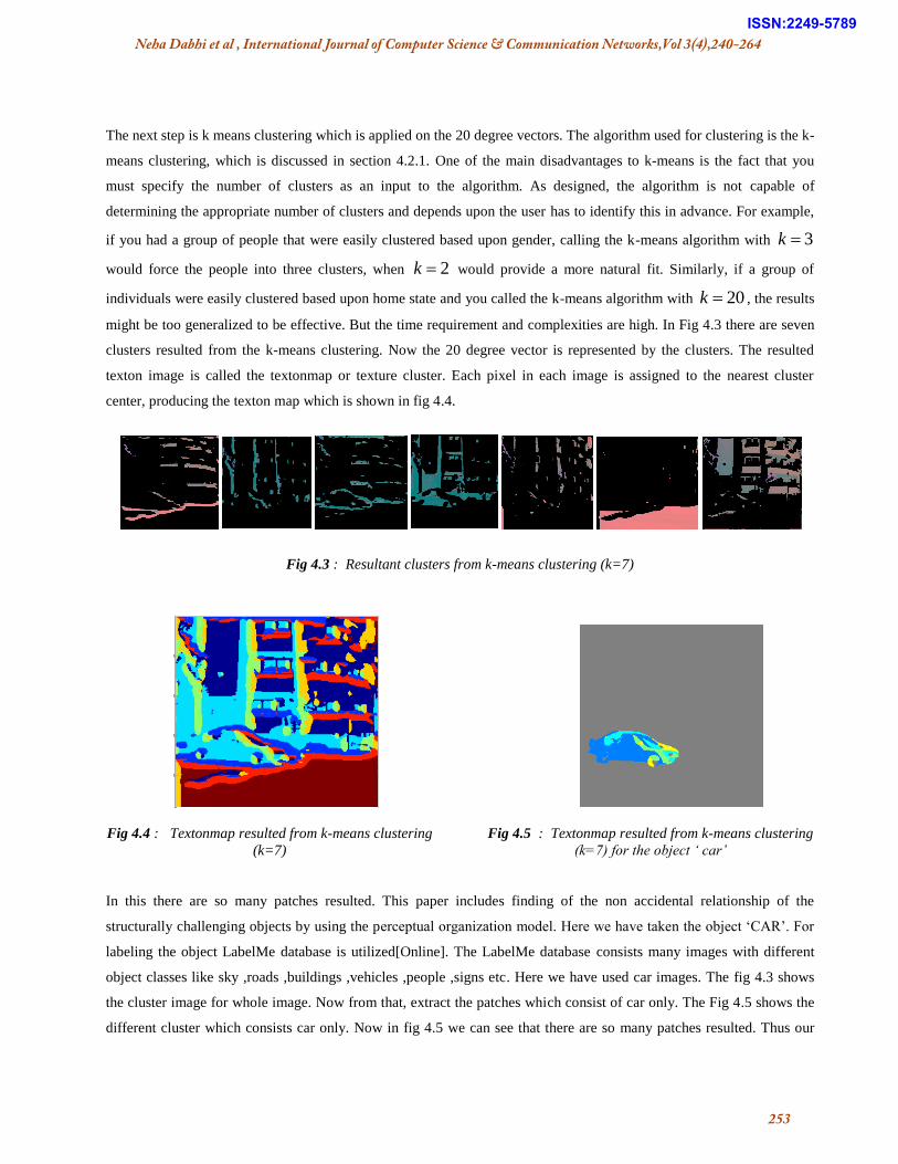
might be too generalized to be effective. But the time requirement and complexities are high. In Fig 4.3 there are seven

clusters resulted from the k-means clustering. Now the 20 degree vector is represented by the clusters. The resulted

texton image is called the textonmap or texture cluster. Each pixel in each image is assigned to the nearest cluster

center, producing the texton map which is shown in fig 4.4.

Fig 4.3 : Resultant clusters from k-means clustering (k=7)

Fig 4.4 : Textonmap resulted from k-means clustering

(k=7)

Fig 4.5 : Textonmap resulted from k-means clustering

(k=7) for the object ‘ car’

In this there are so many patches resulted. This paper includes finding of the non accidental relationship of the

structurally challenging objects by using the perceptual organization model. Here we have taken the object ‗CAR‘. For

labeling the object LabelMe database is utilized[Online]. The LabelMe database consists many images with different

object classes like sky ,roads ,buildings ,vehicles ,people ,signs etc. Here we have used car images. The fig 4.3 shows

the cluster image for whole image. Now from that, extract the patches which consist of car only. The Fig 4.5 shows the

different cluster which consists car only. Now in fig 4.5 we can see that there are so many patches resulted. Thus our

50 100 150 200 250

50

100

150

200


253

ISSN:2249-5789

aim is to merge all those patches and recognize car as one object so we can achieve the performance close to the human

vision, which is the central idea of this dissertation.

In fig 4.6 (a) we can see that the car is segmented into many patches it is low level segmentation but the human can

identify the car as one whole object. Thus, POM works on the principle that it identifies the structural relationship

between the constituent parts of an object and grouped them together.

Fig 4.6 : Principle of POM

The result of textonization process can be visualized in above Fig 4.5. There are so many patches in the background are

there .So here we have subtracted the background and extracted the desired object. Also the Car is not segmented into

one object and it is partitioned into many patches. Therefore, the rest of section describe sthe grouping of this multiple

clusters.

4.2 Boosting based object classification.

In this section we present the experimental results for boosting based object classification algorithm for the outdoor

environment and object classification method on the LabelMe and ICCV database. The images cover various

environments like urban areas, suburban areas, residence areas, roads, airports, etc. and it contains the variety of object

classes like skies, roads, buildings, vehicles, vegetation, people, signs, cars etc… Here generation of the single scale

boosting detector is carried out. In this experimentation the LabelMe toolbox [Online] is utilized.

The very first step is to generate the annotations of the images and create the database of the training images and

annotations .That is done by LabelMe tool provided on the website [Online].

In this we have learned the two objects named as : ‗car+side-part-occuluded‘.There are handpicked set of filters

Laplacian, x derivative and y derivative which extract the features from the images and also the original image. The

masks of the filter are as per discussed in section 5.4. Here,edge based filters are utilized, as edges are good texture

signature. In this the image is retrieved based on the sample image queries. Initially, there are 8 samples of images are

utilized to build the dictionary of patches. There are 20 numbers of patches extracted from every image. The size of the

(a) (b)


254

ISSN:2249-5789

training image is [128 200] .There are 30 background samples are extracted from every image. The size of the test

image is [256 256].Now, there are 50 images are used here for training. Thus ,here total no of filters are 4 (Laplacian, x

derivative and y derivative and original imge) from which the patches are extracted from every example are 20 thus

total 80 patches are extracted from every image,which are shown in below Fig 4.7

Then, we have created the annotations of the images. Here,the annotation which consist the ground truth of the images

created from LabelMe web is taken which are further used.Then the next step is to create the dictionary of features.

From each object class get 10 images, which are normalized in size. Then filter the image with one filter (3 filters –x

derivative, y derivative and laplacian), thus there are 9 outputs resulted. Then fragment sampling location on a regular

grid 3x3.Thus, there are 10x3x9=270 fragments are resulted from each object. Now store indices of images used for

building dictionary.

Fig 4.8 : (a)new annotation of the tightly cropped

centered object

(b)Color segmented mask

Fig 4.7 : Extraction of the patches

The next step is to crop the desired object from the image and create mask of the desired object which will be further

utilized in foreground and background binary identification process. Now, pre-compute the features of all images and

store the feature output on the centre of the target object and on sparse set of location from the background. Here there

is one loop which finds the sample location for negative examples where the template produces the strong false

alarms.Thus in the resultant image the one red square represents the centre of the detected object and 30 green square

represents the background objects. In this binary categorization is used thus the detected object has +1 class and

background objects have -1 class.

50 100 150

-100

-50

0

50

100

150

200

carside

50 100 150

20

40

60

80

100

51015

51015246810

246810510152025

51015202524681012

24681012510152025

510152025510152025

5101520255101520

5101520510152025

5101520252468

2468

510152025

5101520252468

246824681012

2468101251015

51015510152025

51015202551015

5101524681012

24681012246810

246810246810

246810

24681012

2468101251015

5101551015

5101551015

5101551015

5101551015

510152468

24682468

246851015

51015

510152025

51015202551015

51015510152025

51015202524681012

2468101224681012

246810125101520

51015205101520

510152051015

510155101520

5101520

51015

5101551015

5101551015

5101551015

510155101520

51015202468

24685101520

5101520246810

24681051015

51015

24681012

2468101251015

5101524681012

24681012510152025

5101520252468

2468246810

24681051015

5101524681012

24681012246810

246810

246810

246810510152025

51015202524681012

2468101224681012

2468101251015

510152468

24682468

246824681012

2468101224681012

24681012

5101520

51015205101520

51015205101520

510152051015

5101551015

5101551015

510155101520

510152051015

5101551015

51015

51015

5101524681012

246810122468

246851015

51015246810

24681051015

510155101520

510152051015

51015


255

ISSN:2249-5789

(a) (b) (c)

Fig4.9: Binary categorization of the image

Now train the detector by the help of training data and features generated as above and selected 120 weak classifiers. In

the gentleboost classifier D(i) is the weight for each training sample, which determine the probability of being selected

for a training set for an individual component classifier. Initially, we have given uniform weight across the training set.

Now at each round we find a classifier that will minimize the error with respect to distribution. In the next round we will

assign the higher weight to the misclassified data and less weight to the correctly classified data. Thus,the new

distribution is used to train the next classifier and the process is iterated up to 120, because we have selected 120 weak

classifiers.

Fig 4.10 : Output of the detector

Fig 4.11 : Precision Recall Curve

Here ,single scale boosted detector algorithm is utilized ,it runs the strong classifier on an image at a single scale and

outputs the bounding boxes and scores which are used to find the point on the precision recall curve. And then the final

output which contains the classified object is plotted .According to the object classification the true alarm or false alarm

resulted, which shows correct classified object or misclassified object which are shown in Fig 4.10. While the Fig 4.11

shows the precision – recall curve for 120 learners. Here , we can see that there are two cars in that image from them the

one car is correctly classified while the other cannot be classified so the false alarm is there.


256

ISSN:2249-5789

4.3 POM based segmentation

As discussed in section 3.4 the relationship between the constituent parts of an object and then merging is carried out

based on two parameters: Cohesive Strength and energy.

In the algorithm we have selected one reference patch a then checked the neighborhood of all patches with each other

in an image and found the vector v which contains the connected component with the image patch i . Then, the laws

applied on that patch and calculated the cohesive strength is calculated from equation 4.4 and the energy is calculated as

per section 3.4.2. Then we have established the energy criteria and cohesive strength criteria as below based on that the

merging process is carried out.

Condition:

Cohesive Strength Criteria: Cohesive Strength > 0.85

Energy Boundary Criteria: )(())(( aa REvRE

Here, aR is the boundary which contains the reference patch a .If this condition is fulfilled then the region will be

merged and if it is not fulfilled then select next neighbor. Finally store all the data for next round and repeat the process.

Similarly, for cohesive strength if cohesive strength > 0.85 then merge patches otherwise select next patch. Finally store

all the data for next round and repeat the process.

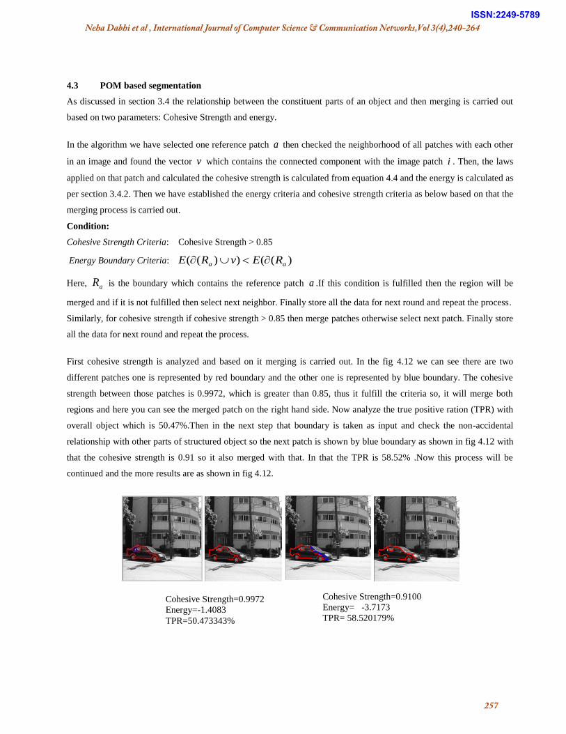
First cohesive strength is analyzed and based on it merging is carried out. In the fig 4.12 we can see there are two

different patches one is represented by red boundary and the other one is represented by blue boundary. The cohesive

strength between those patches is 0.9972, which is greater than 0.85, thus it fulfill the criteria so, it will merge both

regions and here you can see the merged patch on the right hand side. Now analyze the true positive ration (TPR) with

overall object which is 50.47%.Then in the next step that boundary is taken as input and check the non-accidental

relationship with other parts of structured object so the next patch is shown by blue boundary as shown in fig 4.12 with

that the cohesive strength is 0.91 so it also merged with that. In that the TPR is 58.52% .Now this process will be

continued and the more results are as shown in fig 4.12.

Cohesive Strength=0.9972

Energy=-1.4083

TPR=50.473343%


Energy= -3.7173

TPR= 58.520179%


257

ISSN:2249-5789

Fig 4.12: First Round of POM (Merging based on cohesive strength)

Now, the boundary energy based merging of the patch is as follows. Here ,in fig 5.12 beside the patches there is box

which shows the parameter extracted from that patch. For fist one the cohesive strength is 0.9972 but the boundary

energy is -1.4083 which is greater than the energy of the reference patch which is -1.7323 so they will not merge . Now

the next patch is taken, it will find the energy of that patch with its neighboring patch which is shown in Fig 5.13 by

blue boundary which is -3.7173 which is less than the boundary energy of the reference patch, so they both merge. Thus

this process is continued .The results are shown in Fig 5.13.

The fig 4.14 shows the final result of the segmentation after round 1 . We can see that we can achieve the good result in

cohesive strength based merging criteria. In the energy based phenomenon there are so many patches remaining .It is

observed that part is weakly attached so it cannot group together with the whole.

Energy= -3.7173 , TPR = 56.020% Energy= -3.4209 , TPR = 59.267%


Energy= -3.4209

TPR= 60.712506%


Energy= -1.6338

TPR= 64.798206%


Energy= -2.9666

TPR =66.317887%


258

ISSN:2249-5789

Energy= -2.9666 , TPR = 62.381% Energy = -3.0587 , TPR= 63.278%

Fig 4.13: First Round of POM (Merging based on Energy Boundary)

The fig 4.14 shows the final result of the segmentation after round 1 . We can see that we can achieve the good result in

cohesive strength based merging criteria. In the energy based phenomenon there are so many patches remaining .It is

observed that part is weakly attached so it cannot group together with the whole.

Fig 4.14 : Comparison after Round 1 (a) Output of Cohesive strength (b)Output of Boundary Energy

Now, above result is the input of second round.The fig 4.15 shows the other patches merged with the boundary

extracted from the first round .here we can see that the cohesive strength wise they can merge but they do not follow the

energy criteria so they will not merge.

Fig 4.15 : Patch merging in second round


Energy=-0.6890


Energy=- -1.3804


259

ISSN:2249-5789

Fig 4.16 : Intermediate result in second round a) Cohesive strength based

b) Boundary Energy based

The fig 4.16 shows the intermediate results of the ‗car‘ .Now, merge the patches until there is no patch remaining

without merging which is connected with the other based on both parameter cohesive strength and energy .The final

output is shown in Fig 4.17.

Fig 4.17: Final result a) Cohesive Strength based b) Boundary Energy based

(a) (b)

(a) (b)

(a) (b) (Contd..)


260

ISSN:2249-5789

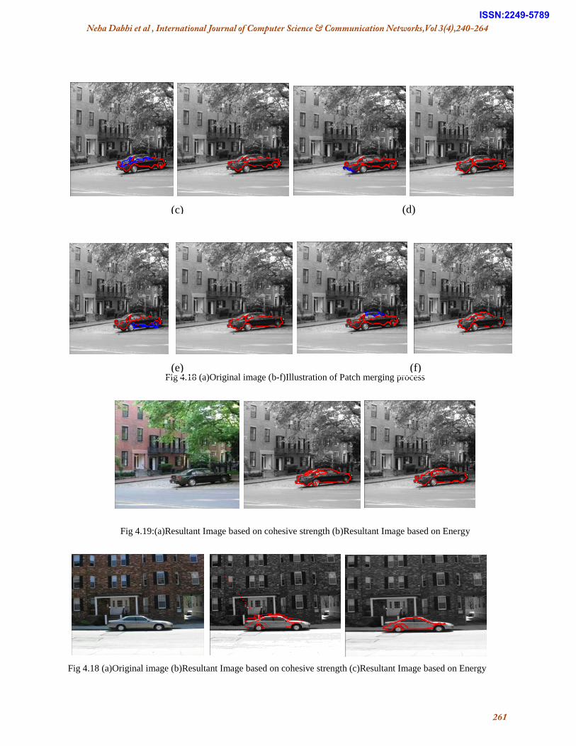
Fig 4.18 (a)Original image (b-f)Illustration of Patch merging process

Fig 4.19:(a)Resultant Image based on cohesive strength (b)Resultant Image based on Energy

Fig 4.18 (a)Original image (b)Resultant Image based on cohesive strength (c)Resultant Image based on Energy

original RGB image

(c) (d)

(e) (f)


261

ISSN:2249-5789

5.4 Evaluation

Now, here the performance analysis is carried out based on TPR. At iteration 1 there are two patches (patch 11 and

patch 4), we have checked here the symmetry, alignment & attachment and calculated the cohesive strength as equation

4.4. Then cohesiveness is higher than 85% with each other so they both merged. Now, we will see the boundary energy,

it is based on shape complexity function which is discussed in section 3.4. Then, the shape complexity is higher so they

will not merged. Now, next time that merged patch is utilized and the next one is patch 5 is taken again same procedure

is carried out. At that stage the cohesive strength is 58.520% . And for energy, initially two patches (patch 11 and patch

5) have taken then calculated the energy as equation 4.9.The shape complexity is lesser in this so, they fulfill the

condition which is discussed in section 5.3 so they both merge at that time the TPR is 56.020% for whole image which

is lesser compared to cohesive strength which is 58.520% which can be analyzed in below table so TPR is less because

here the 4th

patch is not merged. This process will be continued until it finds any structural relationship with the

neighboring patch and they will be merged which is discussed above. Table 5.1 contains the performance analysis and

patch merging process for the input image. In that Outboundary1 is the merged patch in the first round.

Similarly,Outboundary2 is the merged patch in the second round. We can analyzed from Table 5.1 that there were some

patches still there in merging based on cohesive strength but not in boundary energy based merging .So ,finally we got

higher TPR value in case of cohesive-strength compared with boundary energy.

Table 5.1: Performance analysis

POM

Round

Merged patch based

on Cohesive Strength

Cohesive Strength Merged patch

based on Boundary

energy

Boundary Energy

First Round {11,4,5} 58.520% {11,5} 56.020%

{11,4,5,7} 60.712% {11,5,7} 59.267%

{11,4,5,7,8,9} 66.317% {11,5,7,9} 62.381%

{11,4,5,7,8,9,15} 67.090% {11,5,7,9,15} 63.278%

Second

Round

{Outboundary1,12,14} 72.820% {Outboundary1} 63.278%

Third Round {Outboundary2,2,6} 76.332% {Outboundary1} 63.278%


262

ISSN:2249-5789

Conclusion:

This dissertation is motivated by the need of human visual system based segmentation. The block diagram of outdoor

scene segmentation carries image textonization module for recognizing the appearance based information from the

scene,Feature selection module for extraction of features for training the classifier, Boosting for classifying the objects

from the scene and finally Perceptual Organization Model for merging multiple segmentation of the particular

object.The image segmentation algorithm is based on a Perceptual Organization model. The Perceptual Organization

model can ‗perceive‘ the special structural relations among the constituent parts of an unknown object and hence can

group them together without object-specific knowledge. The results of proposed image segmentation based on POM

process can be visualized and analyzed with both cohesive strength and boundary energy parameter. As we can see in

this, the cohesive strength based POM gives good result compared with the boundary energy parameter. Here we have

taken the object ‗CAR‘ which is not merged into one object. But it tries to merge into one but the patches which are not

connected with each other, they cannot merge. So, we can get above result.The experimental result shows that, it works

well with the structurally challenging objects, which usually consist of multiple constituent part and also gives the

performance close to human vision. So, the prediction of human eye fixation can be done.

Future work:

In this paper the merging of patches is based on geometrical laws and the singularity of curve features can be described

by its frequency and strength (amplitude). In this we have computed amplitude of boundary complexity function based

on fixed window length . So, include sliding window with variable window based concept in shape complexity

estimation and then analyze the performance of the model then it can improve the results . This paper concentrated on

merging the patches based on mid level cues which are Gestalt Laws – Symmetry , Alignment , Attachment ,

Continuity.Thus, to improve the performance include more laws and also include some other cues into the model.

References :

Books:

[Gonazalez,Woods]Rafel C. Gonazalez , Richard E.Woods, Digital Image Processing,Pearson Publication.

Web sites:

[Online] Available: http://people.csail.mit.edu/torralba/LabelMeToolbox/

Journal articles

[Shah,2008] S. K. Shah, Performance modeling and algorithm characterization for robust image segmentation, Int. J.

Comput. Vis., vol. 80, no. 1, pp. 92–103, Oct. 2008.

[Winn et al., 2005] J. Winn, A. Criminisi, and T. Minka, Categorization by learned universal visual dictionary, in Proc.

IEEE ICCV, 2005, vol. 2, pp. 1800–1807.

[Gould et al., 2008] S. Gould, J. Rodgers, D. Cohen, G. Elidan, and D. Koller, Multiclass segmentation with relative

location prior,‖ Int. J. Comput. Vis., vol. 80, no. 3, pp. 300–316, Dec. 2008.

[Shotton et al.,2009] J. Shotton, J. Winn, C. Rother, and A. Criminisi, Textonboost for image understanding: Multi-class

object recognition and segmentation by jointly modeling texture, layout, and context, Int. J. Comput. Vis.,vol. 81, no. 1,

pp. 2–23, Jan. 2009.


263

ISSN:2249-5789

http://people.csail.mit.edu/torralba/LabelMeToolbox/

[Luo & Guo ,2003] Jiebo Luo ,Cheng-en Guo ,‖perceptual grouping of segmented regions in color images‖, in the

journal of pattern recognition society published by Elsevier Ltd., Volume 36, Issue 12, December 2003, Pages 2781–

2792

[Martin et al ,2004] D. R. Martin, C. C. Fowlkes, and J. Malik, ―Learning to detect natural image boundaries using local

brightness, color, and texture cues,‖ IEEE Trans. Pattern Anal. Mach. Intell., vol. 26, no. 5, pp. 530–549, May 2004.

[Cheng et al.,2012]C. Cheng, A. Koschan, D. L. Page, and M. A. Abidi, Outdoor scene image segmentation based on

background recognition and perceptual organization, in Proc. IEEE Trans, vol.21, no.3,pp. 1007–1019, March2012.

[Kang et. Al.,2008] Yousun Kang,Kidono,Naito,Nimoniya,‖Multiband Image segmentation and object recognition

using texture filter banks‖ In 19th International Conference on Pattern Recognition (ICPR 2008), December 8-11, 2008,

Tampa, Florida, USA. pages 1-4, IEEE, 2008.

[Julesz,1981]B. Julesz,‖Textons-the elements of texture perception and their interactions‖ ,Nature , vol. 290, no. 5802,

pp. 91-97, 1981

[Xuming He&Zemel,2006]Xuming He, Richard S. Zemel, and Debajyoti Ray. 2006,‖ Learning and incorporating top-

down cues in image segmentation‖. In Proceedings of the 9th European conference on Computer Vision - Volume Part

I (ECCV'06), Aleš Leonardis, Horst Bischof, and Axel Pinz (Eds.), Vol. Part I. Springer-Verlag, Berlin, Heidelberg,

338-351. DOI=10.1007/11744023_27 http://dx.doi.org/10.1007/11744023_27

[Varma,2005] Varma, M., Zisserman, A., A statistical approach to texture classification from single images.

International Journal of Computer Vision: Special Issue on Texture Analysis and Synthesis Volume 62 Issue 1-2, April-

May 2005 ,Pages 61 – 81

[Leung,2001]T.Leung , J. Malik , Representing and recognizing the visual appearance of materials using three-

dimensional textons ,International Journal of Computer Vision (IJCV) , vol. 43, no. 1, pp. 29-44, 2001

Conference :

[Sharma & Davis ,2007] Sharma & Davis ,‖Integrating appearance and motion cues for simultaneous detection and

segmentation of pedistrician‖ ,in IEEE International Conference on Computer Vision,Rio de Janerio, Brazil , October ,

2007

[Kootstra et al,2010]G. Kootstra, N. Bergstrom, and D. Kragic, ―Using symmetry to select fixation points for

segmentation,‖ in Proceedings of the International Conference on Pattern Recognition, 2010.


264

ISSN:2249-5789

outdoor scene segmentation and object classification the appearance based information from the...

Documents