Our Fans In The North: The Demandfor British Rugby League

by

J.C.H. Jones, J.A. Schofield and D.E.A. Giles*

University of Victoria, Victoria, British ColumbiaDepartment Of Economics, PO Box 1700, STN CSC, V8W 2Y2,

Canada

Abstract

This paper reports the results of estimating a single equation model of an attendance function forBritish Rugby League over the seasons 1982/83 to 1990/91. The data are panel data coveringvirtually every team which played in the two division league over the nine year time period. Diagnostic tests indicate that the appropriate model is a semi-log random effects model, where thedependent variable is league attendance weighted by population. The major results are as follows:there are significant positive relationships between league attendance and various measure of teamsuccess (although the direction of causality is moot), team quality (as proxied by the two divisions)and the economic quality of team location (as proxied by the unemployment rate); but there is nodiscernible relationship between league attendance and either success in non-league trophycompetitions or measures of exceptional player quality.

* The authors are Professors of Economics

2

I. Introduction

In the literature on professional team sport a standard empirical exercise has been to

estimate a demand function. Typically, single equation models are estimated using OLS

techniques, where attendance is the endogenous variable and the exogenous variables are some

combination (depending on data availability) of factors common to all demand studies (price,

income, etc.) and specific to team sports (team success, outcome uncertainty). The results are

then used to address a variety of behavioural and policy issues which range from, considering

whether teams maximize profits, through determining the optimum structure of a league, to

assessing the viability of individual teams.1

Unfortunately, and almost inevitably given the emergence of better data sets and the

advances in econometric testing, few of these studies are free from criticisms of one kind or

another and the result is that the whole literature has the feel of a work in progress. For

instance, studies using time series data and OLS procedures tend to gloss over the difficulties

that arise from the potential lack of stationarity in the data and so risk introducing spurious

regression problems into the estimates. This, in turn, means that the empirical results may be

seriously flawed, rendering the behavioral and policy inferences highly suspect.

Consider, for example, the case of British Rugby League. On the one hand, Burkitt

and Cameron (1992) use OLS procedures to estimate an attendance function from time series

data (1966-1990), but fail to test for stationarity. From their results they deduce that team

success is a positive determinant of attendance, and the 1973 restructuring of the league into

two divisions could be considered a modest success in promoting both league and team

viability. On the other hand, Davies, Downward and Jackson (1995), correcting for the lack of

stationarity in their own data and using a VAR model to estimate another attendance function,

3come to opposite conclusions: attendance drives team success; there is no evidence that the

league restructuring scheme was a success; and the best way of ensuring league survival is to,

“develop the grassroots of the game via the amateur network” (p.1007).

Since the econometrics of the study by Davies et al. are more sophisticated than those

employed by Burkitt and Cameron there is a temptation to accept the former results at face

value. Yet, the Davies et al. study raises three areas of concern. First, the data base is quite

limited, comprising a panel of only five teams which have existed continuously in the First

Division from 1964 to 1993. These teams cover a fraction of the thirty plus teams operating in

any one season during this period and, hence, questions arise about the representativeness of

the sample. Second, the model courts serious misspecification confined as it is to, basically,

one endogenous (attendance) and one exogenous (team success) variable. Third, there is a

surprising lack of reported diagnostic testing, given that the criticisms of Burkitt and Cameron

by Davies et al. are principally econometric in nature. It is important, therefore, to address

these three areas of concern before accepting Davies et al.’s conclusions, and by inference

rejecting those of Burkitt and Cameron.

Accordingly, the object of this paper is to reconsider the demand for rugby league by

estimating an attendance function for the seasons 1982/83 to 1990/91 inclusive. Our research

methodology is to estimate a single equation, multi-variable model using panel data covering

virtually every team that played in the first and second division over this time period; and to

subject the model to extensive diagnostic testing. From the analytical point of view the time

period has the advantage of being one of relative structural stability in the league: two divisions

operated throughout and the number of new team entries and exits was at an absolute

minimum. This contrasts with the post-1991 era when the number of divisions jumped from

4two to three then back to two, a Super League was introduced and the season shifted from

Fall and Winter to Summer.

Our major conclusions are as follows. First, the most appropriate model for analyzing

variations in league attendance in this time period is a random effects model in which the

dependent variable is attendance weighted by market population (attendance per capita) rather

than the more conventional attendance (unweighted). Second, of the exogenous variables,

“team success” is an important determinant of attendance; but the success associated with

“trophy” competitions did not translate into increased league attendance. Third, “team quality”

(as proxied by first and second divisions teams) and economic “market quality” (proxied by the

unemployment rate) are also significant determinants of attendance. Finally, all of these

conclusions depend crucially on a series of diagnostic tests on which the final form of the

estimated model is based. Without them, it is fair to say that the statistical results would be

questionable and the associated inferences defective.

The remainder of the paper details the rationale for these conclusions: section II

outlines the model; section III considers the empirical analysis; and section IV offers extended

conclusions.

II. The Model

The regression model underlying our analysis is a variation on a fairly standard

approach to estimating the demand for team sport using annual time series data. Our intention

is to estimate a single equation model using panel data where team attendance is determined by

a series of exogenous variables representing team success and player, team and locational

quality. The most critical factor governing the model’s empirical content is data availability

and the complete model is summarized by equation (1).

5(1) ATT=α 0 +α 1LPS + α 2LPP + α 3PZS + α 4PZP + α 5RZS + α 6RZP +

α 7CCWS + α 8CCWP + α 9CCFS + α 10CCFP + α 11CCSS + α 12YCWS + α 13YCWP + α 14YCFS + α 15YCFP + α 16LCWS + α 17LCWP +α 18LCFS + α 19LCFP + α 20RTWS + α 21RTWP + α 22RTFS + α 23RTFP + α 24RTSS + α 25PWS + α 26PWP + α 27PFS + α 28PFP + α 29PQS + α 30MAN + α 31BEST +α 32DD +α 33POP+ α 34UEM+ α 35RAIN+α 36TEMP+ε .

The dependent variable, ATT, is average league attendance by game (total league

attendance per season divided by the number of home games) by team. The independent

variables can be broadly grouped into measures of: team success, either in the current or

preceding season in either league (α 1 to α 6) or “trophy” (α 7 to α 29) play; superior player

quality (α 30 and α 31); the difference in overall team quality between first and second divisions

(α 32); and the quality of specific team locations (α 33 to α36). The error term is denoted as ε.

More precise definitions of the variables, their construction and the basic data sources appear

in Table 1 and the footnote below.2

On a priori grounds we anticipate the following relationships. The standard

expectation is that ATT will be positively related to team success in league competition in both

current and previous seasons (α 1, α 2 >0). Nevertheless, if the results reported by Davies et

al. (1995) are indicative, causation runs from attendance to success. The argument,

presumably, is that large crowds produce more revenue which can be spent on better players

which, in turn, leads to increased team success.

The coefficients of the promotion zone dummies should be unequivocally positive (α 3,

α 4>0) , because these variables represent successful involvement in a more meaningful

Table 1Variable Definitions

ATT = average attendance per league gameLPS = league performance of same year, percentage of maximum league points the same year.

6LPP = league performance of previous year, percentage of maximum league points the previous yearPZS = promotion zone dummy of 1 (0 otherwise), if the team was in the “promotion zone”

(i.e. top 6 ranked teams prior to 1985; top 4 ranked teams 1986-87; top 5 ranked teams post 1986-87) of the second division in the same year.

PZP = promotion zone dummy of 1 (0 otherwise), if the team was in the “promotion zone” the previous year.RZS = relegation zone dummy of 1 (0 otherwise), if the team was in the “relegation zone” (i.e.

bottom 6 ranked teams except for 1985-86; bottom 5 ranked teams post 1985/86 of the first division in the same year.

RZP = relegation zone dummy of 1 (0 otherwise), if the team was in the relegation zone the previous year.

CCWS = Challenge Cup dummy of 1(0 otherwise) if the team was a winner in the same year.CCWP = Challenge Cup dummy of 1 (0 otherwise) if the team was a winner the previous year.CCFS = Challenge Cup dummy of 1 (0 otherwise) if the team was a finalist the same year.CCFP = Challenge Cup dummy of 1 (0 otherwise) if the team was a finalist the previous year.CCSS = Challenge Cup dummy of 1 (o otherwise) if the team was a semi-finalist the same year.YCWS = Yorks Cup dummy of 1 (0 otherwise) if the team is a winner in the same year.YCWP = Yorks Cup dummy of 1 (0 otherwise) if the team is a winner in the previous year.YCFS = Yorks Cup dummy of 1 (0 otherwise) if the team was a finalist the same year.YCFP = Yorks Cup dummy of 1 (0 otherwise) if the team was a finalist the previous year.LCWS = Lancs Cup dummy of 1 (0 otherwise) if the team is a winner in the same year.LCWP = Lancs Cup dummy of 1 (0 otherwise) if the team is a winner in the previous year.LCFS = Lancs Cup dummy of 1 (0 otherwise) if the team was a finalist the same year.LCFP = Lancs Cup dummy of 1 (0 otherwise) if the team was a finalist the previous year.RTWS = Regal Trophy dummy of 1 (0 otherwise) if the team is a winner in the same year.RTWP = Regal Trophy dummy of 1 (0 otherwise) if the team is a winner in the previous year.RTFS = Regal Trophy dummy of 1 (0 otherwise) if the team was a finalist the same year.RTFP = Regal Trophy dummy of 1 (0 otherwise) if the team was a finalist the previous year.RTSS = Regal Trophy dummy of 1 (0 otherwise) if the team was a semi-finalist the same year.PWS = Premiership dummy of 1 (0 otherwise) if the team was a winner in the same year.PWP = Premiership dummy of 1 (0 otherwise) if the team was a winner in the previous year.PFS = Premiership dummy of 1 (0 otherwise) if the team was a finalist the same year.PFP = Premiership dummy of 1 (0 otherwise) if the team was a finalist the previous year.PQS = Premiership dummy of 1 (o otherwise) if the team was a quarter finalist the same year.MAN = superstar dummy of 1 (0 otherwise) if winner of the Man of Steel award is a member of

the team.BEST = superstar dummy of 1 (0 otherwise) if winner of the Best Division Player (for each

division) is a member of the team.DD = division dummy of 1 (0 otherwise) if the team plays in the first division.POP = population (mean), two year average (000).UEM = unemployment rate.TEMP = average yearly temperature (c), Sept through March.RAIN = average yearly rainfall (mm), Sept through March.“contest within a contest” where the outcome is even more uncertain. By the same token, the

relegation zone dummies should also be positive (α 5, α 6>0) , since this is a contest, replete

with its own attendant uncertainties, to see who stays in the first-division. Of course, the

7reverse could be true: exceptionally poor league performance could be rewarded by reduced

attendance despite the increased uncertainty over the outcome.

As far as the “trophy” competitions are concerned we anticipate that success in these

contests will have a positive impact on league attendance (α7 to α29>0). In effect, success in

cup competition acts as a positive externality for attendance at league games. However,

whether some competitions − the Challenge Cup, Yorkshire Cup, Lancashire Cup, Regal

Trophy, Premiership − are more important than others in this regard, is moot. Likewise, if

there are positive externalities from trophy competitions, are they confined to finalists or are

there positive impacts for semi-finalists or quarter-finalists? These propositions can be tested

by reference to the individual coefficients and also by a series of joint tests for groups of

coefficients.

With regard to player, team and market quality, we expect a positive relationship between

attendance and all measures of quality. As crowds are often drawn to see “superstars”

(presumably the apogee of player quality) irrespective of the performance of the team, we

anticipate that MAN and BEST will be positive (α30 ,α31>0). In addition, as the quality of

team play is likely to be higher in the first division, the divisional dummy variable (DD) should

be positive (α32>0). We also expect the better quality market areas to be positively associated

with attendance. If we proxy “better quality” markets by size (population, POP) and economic

condition (proxied by unemployment, UEM) we expect POP to be positive (α33>0) and UEM

to be negative (α34<0). Lastly, inured as spectators in the north are to bad weather in the Fall

and Winter, we, nevertheless, expect that bad weather, as measured by rain and temperature

(RAIN, TEMP), will negatively (positively) effect attendance (α35<0; α36>0).

8Finally, we should note again that, in common with most statistical work, the content

of the basic estimating equation is determined principally by data availability. In the present

context, some variables which should be included in equation (1) on a priori grounds – ticket

prices, income and competitive entertainments (sporting and otherwise) are the obvious

examples − are omitted because the data are simply unavailable. The data that are available for

variables in equation (1) cover almost every team playing in the first and second divisions over

the period 1982/83 to 1990/91 (for a listing see Appendix Table A1 below). There is a

maximum of 37 and a minimum of 32 teams for any one season, giving a maximum of 309

actual observations in the sample. However, by applying the Ryan-Giles (1998) procedure we

were able to fill in the missing gaps and increase the sample size. Thus, the stationarity and

functional form testing (III (i) and (ii) below), are undertaken with a larger 333 observation

sample using the SHAZAM computer package; but the panel estimations (III (iii), and (iv)

below) are undertaken with a 309 observation sample using the TSP package, because the

panel is “unbalanced,” in the sense that not every time-series observation is available for every

cross-section data point.

Given the content of equation (1) we now turn to the empirical analysis.

III. Empirical Analysis

The empirical analysis of the model in equation (1) proceeds in the following sequential

steps: (i), the data are tested for stationarity; (ii), the specification of equation (1) is tested for

functional form and the most appropriate form is selected; and (iii), the interactive effects of

the panel data are tested via a series of regression models of (ii) representing the between,

fixed, and random effects of the data, and the most appropriate form of the basic model is

9selected; and (iv) in light of the model selected in (iii), the a priori expectations developed in I

are considered.

(i) Non-Stationarity Testing

Table 2 shows the results of the non-stationarity tests for the non-dummy variables in

equation (1) using the panel sample of 333 observations. Given the panel nature of the data,

the usual single-series unit root tests, such as those of Dickey and Fuller (1981), are not

applicable. Various alternative tests have been suggested for this situation (for example,

Table 2Stationarity Results

Variable No Drift/No Trend Drift/No Trend Drift/Trendt-ratio * t-ratio * t-ratio *

Attendance -1.73 -45.13 -43.55

Population -22.93 -34.17 -8.29Unemployment -6.74 2.62 -10.36LeaguePerformance(same year)

-3.62 -18.57 -20.74

LeaguePerformance(previous year)

-2.63 -18.92 -22.71

Temperature -2.01 -50.69 -46.29Rain -1.80 -64.64 -56.27

LAPC 1 0.69 -10.54 -15.55

1. Log of Attendance/Population. See text and Tables 2 and 3 below* The critical value is -1.645 for a at 5% one-tail test.

Karlsson and Löthgren, (1999)), and we have used the testing procedure proposed by Wirjanto

(1996) to investigate the stationarity properties of our data. Wirjanto’s test statistic is

asymptotically standard Normally distributed, and as can be seen in Table 2, the null of a unit-

root is clearly rejected. Thus, the data need not be adjusted for non-stationarity prior to

estimating equation (1).

10

(ii) Functional Form

Table 3 reports some basic diagnostic tests from estimating equation (1) using various

functional forms. These are based on OLS estimation with White’s (1980) heteroskedasticity -

consistent covariance matrix as implemented by the SHAZAM computer package. 3 In

comparing models 1 through 4, model 4 (the semi-log specification) is preferred principally on

the grounds that the associated homoskedasticity tests and Ramsey RESET tests are superior

to those of models 1 through 3. Unfortunately, the homoskedasticity tests for model 4 still

suggest that the null of homoskedasticity should be rejected, thus compromising this

specification for analytical purposes.

In an attempt to rectify this problem we adopted a different definition of the dependent

variable in equation (1): attendance per capita (attendance/population, APC) was substituted

for the more standard attendance (ATT) used in models 1 through 4. In addition, population

(POP) was removed as an exogenous variable. Diagnostic tests from estimating alternative

functional forms of this revised model revealed that the semi-log form (LAPC) was preferred.

The diagnostic tests of this semi-log form are shown as model 5 in Table 3. The

homoskedasticity tests of model 5 confirm, in contrast to model 4, an absence of

heteroskedasticity. Apparently, the non-linear transformation of the dependent variable has

smoothed out the error variance. This result, coupled with superior RESET and normality

tests, makes model 5 preferred to model 4 on statistical grounds. As these models have

different dependent variable variables, their 2R values cannot be compared.

Table 3

Diagnostic Tests Of Alternative Specification Of Attendance Functions With AttendanceAnd Attendance Per Capita (APC) As Dependent Variable

11

ModelDiagnostic

TestsLinear

DependentVariable

ATT

Log-LogDependentVariable

LATT

Lin-LogDependentVariable

ATT

Semi-Log(Log-Lin)DependentVariable

LATT

Semi-LogDependentVariable

LAPC

(1) (2) (3) (4) (5)2R 0.8491 0.8864 0.8402 0.8912 0.3332

Jacque BeraLM NormalityTest

χ 2

97.8408

(2 d.f.)

4.8335

(2 d.f.)

225.3898

(2 d.f.)

4.3280

(2 d.f.)

3.5262

(2 d.f.)

HomoskedasticityTests:

E**2 On Yhat 52.731 (1 d.f.) 15.241 (1 d.f.) 39.033 (1 d.f.) 14.237 (1 d.f.) 0.112(1 d.f.)

E**2 onYhat**2

40.556(1 d..f.)

15.087(1 d.f.)

27.647(1 d.f.)

14.270(1 d.f.)

0.016(1 d.f.)

E**2 onLog(Yhat**2)

32.538(1 d.f.)

15.327(1 d.f.)

24.298(1 d.f.)

14.139(1 d.f.)

0.230(1 d.f.)

E**2 on X (B-P-G) Test

117.484(36 d.f)

35.130(36 d.f)

99.012(36 d.f)

36.804(36 d.f)

43.153(35 d.f)

Log E**2 onX (Harvey)

χ 2

84.849

(36 d.f)

40.401

(36 d.f)

75.982

(36 d.f)

32.638

(36 d.f)

43.904

(35 d.f)

Abs(E) on X

(Glejser) χ 2

161.808(36 d.f)

44.21(36 d.f)

146.306(36 d.f)

43.951(36 d.f)

43.453(35 d.f)

RESET Tests~ Fν ν1 2,

RESET (2)(ν ν1 2, )

131.560(1, 271)

2.452(1, 271)

120.360(1,271)

0.806(1,271)

0.189 (1, 272)

RESET (3)(ν ν1 2, )

69.326 (2, 270)

11.435(2, 270)

69.613 (2, 270)

0.406(2, 270)

0.147(2, 271)

RESET (4)(ν ν1 2, )

46.046(3, 269)

1.624(3, 269)

46.367(3, 269)

0.824(3, 269)

0.296(3, 270)

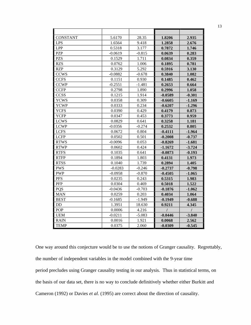
As a further point of comparison, Table 4 shows the complete results of estimating

models 4 and 5. The presence of heteroskedasticity in model 4 obviously renders the levels of

significance of the individual coefficients, highly suspect. While a direct comparison of the

individual coefficients in models 4 and 5 is clearly invidious, it should be noted that there is a

great deal of compatibility between their signs and levels of significance.

12To summarize: in statistical terms, model 5, in which the dependent variable ATT is in

effect weighted by market size (as measured by population), and population is dropped as an

exogenous variable, is the most appropriate form for the study of rugby league attendance in

this time period, and, therefore, serves as the basis for all further estimation in this study.

(iii) Panel Estimates

Taking account of the fact that we have an unbalanced panel of data, Table 5 shows the

results of estimating the fixed, random, and between effects versions of model 5. 4 The

Hausman (1978) test indicates that the random effects model cannot be rejected in favour of

the fixed effects version and so the former becomes the analytical model of choice. A full

range of diagnostic tests, complete with commentary, are shown in Appendix B. Together

they establish that the model is well specified statistically.

(iv) Panel Results

As far as the individual coefficients in Table 5 are concerned the results are mixed. As

anticipated, playing success in the same or previous season (LPS and LPP, respectively) is

positively and significantly related to attendance. However, the issue of the direction of

causality is moot. The fact that LPP is significant and positive suggests some causality from

previous success to attendance. However, the significance of LPS in the same model leaves

open the possibility of bi-directional causality, but does not formally establish its presence.

Table 4

Functional Form: Log ATT (LATT) and Log APC (LAPC)

Model 4 Model 5LATT LAPC

Independent Variables Coefficient t-ratio Coefficient t-ratio

13

CONSTANT 5.6170 28.35 1.8206 2.935LPS 1.6564 9.418 1.2858 2.676LPP 0.5318 3.177 0.7872 1.746PZP -0.0619 -0.815 0.0639 0.283PZS 0.1529 1.711 0.0834 0.359RZS 0.0762 1.006 0.1895 0.781RZP 0.3129 5.292 0.5916 3.130CCWS -0.0882 -0.678 0.3840 1.082CCFS 0.1151 0.930 0.1485 0.462CCWP -0.2551 -1.481 0.2653 0.664CCFP 0.2798 1.890 0.2996 1.058CCSS 0.1215 1.914 -0.0589 -0.301YCWS 0.0358 0.309 -0.6605 -1.169YCWP 0.0333 0.234 -0.6207 -1.296YCFS 0.0390 0.429 0.4179 0.873YCFP 0.0347 0.453 0.3773 0.959LCWS 0.0829 0.641 0.3258 1.181LCWP -0.0356 -0.274 0.2532 0.805LCFS 0.0672 0.804 -0.4111 -1.964LCFP 0.0502 0.501 -0.2008 -0.737RTWS -0.0096 0.053 -0.8269 -1.681RTWP 0.0602 0.424 -1.1672 -3.724RTFS 0.1035 0.641 -0.0873 -0.193RTFP 0.1894 1.803 0.4131 1.973RTSS 0.1040 1.739 0.2894 1.405PWS -0.0283 -0.246 -0.2737 -0.798PWP -0.0958 -0.870 -0.4505 -1.065PFS 0.0235 0.243 0.5315 1.983PFP 0.0304 0.469 0.5018 1.522PQS -0.0436 -0.703 -0.1876 -1.062MAN 0.0259 0.203 0.4034 1.064BEST -0.1685 -1.949 -0.1949 -0.688DD 1.3951 18.630 0.9211 4.345POP 0.0006 4.216 / /UEM -0.0211 -5.083 -0.0446 -3.840RAIN 0.0016 1.921 0.0068 2.562TEMP 0.0375 2.060 -0.0309 -0.545

One way around this conjecture would be to use the notions of Granger causality. Regrettably,

the number of independent variables in the model combined with the 9-year time

period precludes using Granger causality testing in our analysis. Thus in statistical terms, on

the basis of our data set, there is no way to conclude definitively whether either Burkitt and

Cameron (1992) or Davies et al. (1995) are correct about the direction of causality.

14In addition to success in league play, promotion zone competition in the current season

(PZS) has a positive effect on attendance as does relegation zone competition in both

the current (RZS) and, in particular, the previous (RZP) season. These results are as expected.

The results for the “trophy” competitions, however, are somewhat surprising.

Very few of the t-statistics are even greater than 1 and a number of coefficients are

anomalously signed. Joint Wald tests for each competition − Challenge, Yorkshire,

Lancashire, Regal and Premiership − support a conclusion that such competitions are of

relative unimportance for league attendance. All tests (see Table 6) show that the null

hypothesis, that trophy competitions do not have a positive impact on league attendance,

cannot be rejected. Thus, while trophy competitions are undoubtedly revenue producers for

teams there is no evidence that there are any positive external effects on league attendance.

With respect to the quality variables, as hypothesized there is a pronounced difference

between first and second division teams and their impact on attendance (DD). The anticipated

positive individual superstar effects (MAN and BEST) proxying player quality are not

significant and BEST has an incorrect sign. But economic quality as proxied by the

unemployment rate (UEM) is clearly very significant. Finally, good weather (high temperature

and low rainfall) is a positive determinant of attendance. It should be noted, however, that,

although the individual variables (TEMP and RAIN) have the correct signs, they are not

particularly statistically significant.

Table 5

TSP Panel: Dependent Variable Log of Attendance/Population

Plain OLS(Total)

Within Effects(Fixed)

Variance Effects(Random)

Between Effects

Variable Coefficient t-ratio Coefficient t-ratio Coefficient t-ratio Coefficient

t-ratio

15Constant 1.8197 3.0784 1.8675 6.0818LPS 1.2996 2.5525 1.1613 6.6869 1.1735 6.7976 6.1254 0.5489LPP 0.7848 1.6390 0.3323 2.0793 0.3471 2.1779 -6.2546 -0.4738PZS 0.08119 0.3325 0.1359 1.7397 0.1364 1.7505 -1.7599 -0.3232PZP 0.07587 0.3381 -0.0205 -0.2766 -0.0208 -0.2816 0.4926 0.0778RZS 0.1999 0.8034 0.1225 1.5036 0.1240 1.5271 -2.3609 -0.0427RZP 0.5893 3.0525 0.2131 3.2071 0.2270 3.4339 9.9805 0.7379CCWS 0.3933 0.7685 -0.1035 -0.5833 -0.0954 -0.5395 -65.4028 -0.1256CCWP 0.2458 0.4809 0.1069 0.6989 0.1056 0.6918 67.4806 0.1419CCFS 0.1564 0.3419 -0.1604 -1.0001 -0.1556 -0.9711 135.510 0.1576CCFP 0.2916 0.7939 0.1861 1.6130 0.1882 1.6328 -116.073 -0.1745CCSS -0.0549 -0.2073 0.0036 0.0430 0.0037 0.0444 21.4228 0.3864YCWS -0.6486 -1.2997 -0.0125 -0.0813 -0.0231 -0.1502 61.5251 0.1529YCWP -0.7105 -1.4636 -0.0554 -0.3716 -0.0646 -0.4338 0.0000 0.0000YCFS 0.3935 1.0649 0.1255 1.0190 0.1328 1.0816 -6.6447 -0.0517YCFP 0.4962 1.3235 0.1224 0.9565 0.1305 1.0232 -24.7599 -0.1306LCWS 0.3212 0.6215 0.2176 1.3433 0.2158 1.3334 87.8996 0.3275LCWP 0.2049 0.3858 0.0964 0.5792 0.0993 0.5973 -48.4601 -0.2008LCFS -0.4018 -1.0964 -0.0529 -0.4265 -0.0582 -0.4709 -25.9323 -0.8093LCFP -0.1454 -0.3676 -0.0488 -0.3835 -0.0513 -0.4040 0.0000 0.0000RTWS -0.8041 -1.4068 -0.0986 -0.5167 -0.1098 -0.5772 89.5967 0.2309RTWP -1.1622 2.1497 -0.0977 -0.5231 -0.1167 -0.6276 -138.809 -0.2624RTFS -0.0871 -0.1998 0.1289 0.93326 0.1236 0.8948 -42.5735 -0.1973RTFP 0.4168 1.1889 0.1342 1.2164 0.1383 1.2556 34.9250 0.1587RTSS 0.2769 1.0145 0.0139 0.1578 0.0189 0.2158 10.6431 0.3686PWS -0.2873 -0.7247 -0.0153 -0.1239 -0.0207 -0.1675 41.8582 0.6736PWP -0.4101 -0.9265 -0.0347 -0.2395 -0.0441 -0.3048 -53.2620 -0.6669PFS 0.5389 1.7206 0.0226 0.2219 0.0319 0.3139 -14.0662 -0.1335PFP 0.4874 1.5587 0.0741 0.7305 0.0812 0.8016 27.7143 0.2343PQS -0.1927 -1.0177 -0.0582 -0.9539 -0.0590 -0.9689 0.4486 0.0983MAN 0.4018 0.9447 0.0259 0.1907 0.0326 0.2412 27.6553 0.1463BEST -0.2141 -0.7339 -0.1026 -1.0931 -0.1026 -1.0940 -7.6513 -0.3629DD 0.9078 3.9771 1.0393 9.7089 1.0504 10.0534 -5.1068 -0.0965UEM -0.0448 -3.6351 -0.3353 -5.5841 -0.0335 -5.6635 0.1754 0.8625RAIN 0.0068 2.5107 -0.0009 -0.7377 -0.007 -0.5642 0.0241 0.9729TEMP -0.0309 -0.5383 0.0406 1.7432 0.0394 1.7057 -0.3317 -0.4584

R 2 0.3348 0.434 0.389 -0.159

Hausman Test ofFixed effects vs.random effects

χ 2 (35)=35.100

p-value=0.4634

Conclusion:Reject fixedeffects forrandom effects

Table 6Joint Tests For The Significance Of Trophy Competitions

Trophies Test Wald Result χ 2

(df)

5 % CriticalValues

Conclusion

Challenge CCWS=CCWP=CCFS=CCSS=0 1.6633(4)

9.4877 Cannot reject the null

Yorks YCWS=YCWP=YCFS=YCFP=0 3.8467 9.4877 Cannot reject the null

16

(4)Lancs LCWS=LCWP=LCFS=LCFP=0 1.4868

(4)9.4877 Cannot reject the null

Regal RTWP=RTFS=RTFP=RTSS=0 8.8756(5)

11.0705 Cannot reject the null

Premiership PWS=PWP=PFS=PFP=PQS=0 6.0157(5)

11.0705 Cannot reject the null

CCWS=CCWP=CCFS=CCSS=YCWS=YCWP=YCFS=YCFP=LCWS=LCWP=LCFS=LCFP=RTWP=RTFS=RTFP=RTSS=PWS=PWP=PFS=PFP=PQS=0

19.2033(22)

33.9244 Cannot reject the null

(IV) Conclusion

There are three conclusions which emerge from the foregoing analysis. The first is a

fairly obvious technical point but, in light of the methods employed in the literature, bears

emphasizing: in single equation models of the demand for team sports using panel data, an

appropriate choice of estimator and use of diagnostic testing are critical. This applies to

considerations of stationarity, model specification and functional form. Without such testing

the data used in estimating the model and the model itself may be inappropriate and, hence, all

of the inferences are questionable.

Thus, Davies et al.’s criticism of Burkitt and Cameron’s failure to test for stationarity is

well taken, although we would argue that the Davies et al. model is misspecified and needs

more rigorous testing. Similarly, before adopting particular functional forms and model

specifications, an array of appropriate diagnostic tests is required. For example, as Table 3 and

4 indicate, comparing models 4 and 5 on the basis of the size of the R 2 and t-statistics − a

fairly standard practice − would result in selecting a specification (model 4) which fails the

tests for homoskedasticity. In fact, the 2R values should not be compared, and the t-statistics

are distorted by heteroskedasticity. This, in turn, renders its high R 2 suspect.

17Second, any empirical study can be improved by more and better quality data. This

current study could be improved by data on price, income and a longer time series on all

variables. As we have only a nine year panel, we cannot be conclusive about the direction of

causation between team success and attendance, because we cannot incorporate Granger

causality tests. By the same token, we do not have sufficient data on the requisite variables to

treat both attendance and playing success as endogenous variables in a multiple equation

demand system.

Our results as they stand are compatible with those of Burkitt and Cameron: playing

success is a highly significant determinant of attendance; and promotion and relegation zone

dummies are also positively related to attendance. Thus, success determines attendance and, as

the two division set-up also increases attendance – without two divisions there would be no

promotion and relegation zones – this suggests that the post 1973 restructuring of the league is

a success, at least over our time period. However, we cannot reject Davies et al.’s

proposition that attendance determines success because our time series does not go back far

enough; and preferably, promotion and relegation zone variables should really be compared

with a time period in which they did not exist (pre-1973).

Third, while more and better data would be useful, our present study does provide

some strong support for a number of standard hypotheses. Team success in its different guises

− with the exception of the hypothesized positive external effect of trophy competitions − is a

significant determinant of attendance. The quality of team play (first and second divisions) is

also positively related to attendance as is the “economic quality” (proxied by the

unemployment rate) of the market. Player quality, as measured by BEST and MAN, is not

significant. But these may not be particularly good measures with time series data, and

18“superstar” effects may be more apparent with cross section (game by game) data. Finally, bad

weather, as anticipated, has a negative impact on attendance.

Clearly, to resolve all of the issues raised by Burkitt and Cameron on the one hand, and

Davies et al. on the other hand, more and better data are necessary. Until then this study is

also part of a literature in progress.

19Endnotes

We wish to thank Betty J. J. Johnson for exceptional research assistance and Josie

Schofield for assistance with data collection.

Since we began this project a number of colleagues have raised the issue of whether

three Canadian academics should be analyzing British Rugby League. This is an apparent

extrapolation of the view, popular in literary and humanist circles in Canada, that one group

should not write about the behaviour of another group, because they rarely get it right or, even

when they do, “voice” is being (mis) appropriated. As none of us has played British Rugby

League, we are sensitive to the criticisms that we may be unable to get it right or that we have

usurped the prerogatives of some more appropriate research group. Our response is twofold.

First, all co-authors were born in the U.K., played rugby (albeit “union” rather than

“league”) and have watched it extensively over the years. We therefore understand and

empathize with the game. More specifically, one co-author was born outside Leeds,

remembers the legendary Lewis Jones performing feats of magic on the rugby league field, still

follows the results from afar and watches the game whenever in the “North.” Another co-

author was born in Wales, developed an early antipathy to “league” (“Y Cynghrair byth, yr

Undeb am byth”), but remembers Lewis Jones’ magic before he (some would say

‘traitorously’) “went North.” The other co-author was born in Sheffield, and is now a New

Zealander who naturally has an encyclopedic knowledge of all things rugby.

Second, we embrace the “Nicol” proposition. Eric Nicol, winner of a Canadian

Governor General’s literary award, was criticized for writing about professional hockey

because “he never played.” His reply, which we endorse, was that, in the last analysis, “you

don’t need to have a baby in order to be a gynecologist” (The Joy of Hockey, p.160).

201 The sports demand literature has been surveyed in Cairns et al. (1986) and Cairns (1990).

Not all studies estimate OLS single equation models (for examples of multiple equation

demand systems in sport see, Jones and Ferguson (1988), Stewart, Ferguson and Jones (1992)

and Cocco and Jones (1997)), although it is more common than not; and the data used ranges

over single and multi seasons (game by game observations and one observation by team by

season, respectively). More recent examples of demand studies for British sports include:

soccer (Dobson and Goddard (1992), and Baimbridge, Cameron and Dawson (1996)); cricket

(Hynds and Smith (1994)); and rugby league (Burkitt and Cameron (1992), Davies,

Downward and Jackson (1995), and Baimbridge, Cameron and Dawson (1995)). There is no

study of rugby union. This undoubtedly reflects the amateurish (deliberately?) reporting of

attendance and financial data for this heretofore “amateur” game. Presumably this will change

with the professionalization of the game. However, the early evidence from both Welsh and

English clubs and their actual and potential insolvencies suggest that, rather than

professionalize the players, they should professionalize their accountants.

2 The data sources and calculations of the variables are as follows: Population (POP) data:

POP is interpolated between 1981 and 1991 for each year and each area from, OPCS, Census

1981, Key Statistics for Urban Areas, Table 1, HMSO, 1984; and OPCS, Census 1991,

Preliminary Report for England and Wales, Table 4, HMSO, 1991, Municipal Yearbook, Vol.

2, 1991. Unemployment (UEM) data: UEM ratio 1981 * regional male + female regional UEM

rate, where UEM ratio=(male UEM 1981)/(male+female regional UEM 1981). OPCS Census

1981, Key Statistics for Urban Areas, Table 3, HMSO, 1984 (for Male UEM 1981). CSO,

Economic Trends, Annual Supplement 1992, Table 22 (for regional male + female UEM each

year). Weather (TEMP and RAIN) data: Met. Office, Monthly Weather Report, Vols. 99-109,

21No. 9-12, 1982-91, HMSO. All other variables are taken directly or calculated from,

Rothman’s Rugby League Yearbook, various editions

3 The basic model selection has been done on the basis of OLS procedures. However, below

we take proper account of the panel data and perform associated diagnostic tests (see (iii) and

Appendix B).

4 A wide range of model specifications – all sub-sets of model 5 – was explored. There was,

however, little real change from the results reported in Table 5. The results may be obtained

from the authors on request.

22

Appendix Table A1:Clubs, Divisions and Number of Observations

Club First Division Second Division

Barrow 4 5Bradford N 9 0Carlisle 1 8Castleford 9 0Featherstone R 8 1Halifax 6 3Hull 9 0Hull K.R. 8 1Leeds 9 0Leigh 6 3Oldham 7 2St. Helens 9 0Warrington 9 0Widnes 9 0Wigan 9 0Workington T 2 7Batley 0 9Blackpool(Trafford from 1989)

0 7

Bramley 0 9Cardiff 0 3Dewsbury 1 8Doncaster 0 9Fulham 1 8Huddersfield 0 9Hunslet 2 7Huyton (Runcorn1984-85)

0 9

Keighley 0 9Rochdale H 9 0Salford 3 6Swinton 2 7Wakefield T 5 4Whitehaven 1 8York (Ryedale) 1 8Kent Invicta(Southend)

0 2

Mansfield(Nottingham)

0 7

Sheffield E 1 6Chorley 0 3

23

Appendix B: Diagnostic Tests With Panel Data

Diagnostic tests for models estimated with panel data are not highly developed, and

apart from the Hausman test for fixed versus random effects (see Table 5), the TSP and other

packages do not include specification tests. However, by “recovering” the residuals after

suitable panel estimation, a range of standard, asymptotically valid, tests can be constructed

quite simply. To ensure that no autocorrelation was present in the residuals, we first re-

estimated the Random Effects model with an appropriate first-order serial correlation

correction. (See the AR1 command in the TSP Reference Manual, pp.29-34). The results are

shown in Table B1, and the associated residuals were then analyzed for any remaining

autocorrelation, for Normality, and for heteroskedasticity.

Diagnostic tests for autocorrelation and Normality appear in Table B2. They were

constructed by regressing the Random Effects residuals associated with each team against a

constant and then using the DIAGNOS command in the SHAZAM package. Both the

Goodness-of-Fit and Jarque-Bera Normality tests are reported, and there is no evidence of

non-Normality at any reasonable significance level. Lagrange Multiplier tests for serial

independence, against alternatives of simple first-order, simple second-order, and general

second-order autocorrelation are also present. The alternative hypotheses in each case allow

for either autoregressive or moving average processes in the errors for each team. Using these

asymptotically valid tests, there is no reason to reject the null of serially independent errors.

A similar approach was adopted to test for homoskedasticity in the residuals from the

original panel data estimation. In this case, residuals were “recovered” for each time-period

(season), allowing for the “unbalanced” nature of the panel. The results of applying a range of

24Table B1

First Order Serial Correlation (AR1) Estimation For “Variance Effects” ModelVariance Effects (Random)

AR1 Adjustment

Variable Coefficient t-ratio

LPS 0.9777 5.9124LPP 0.2462 1.6520PZS 0.1477 2.0664PZP -0.0161 -0.2302RZS 0.0753 1.0009RZP 0.1818 2.8705CCWS -0.0153 -0.0909CCWP -0.0532 -0.3526CCFS 0.07507 0.5392CCFP 0.1109 1.0100CCSS -0.0069 -0.0959YCWS -0.0349 -0.2463YCWP -0.0268 -0.1914YCFS 0.1148 1.0093YCFP 0.0933 0.7762LCWS .01592 1.0523LCWP 0.0392 0.2481LCFS -0.0186 -0.1606LCFP -0.0218 -0.1845RTWS -0.0216 -0.1268RTWP -0.0039 -0.0224RTFS 0.0981 0.7999RTFP 0.0553 0.5527RTSS -0.0081 -0.1068PWS -0.0123 -0.1099PWP -0.0199 -01494PFS 0.0267 0.2840PFP 0.0659 0.6938PQS -0.0468 -0.8389MAN -0.112 -0.0947BEST -0.0961 -1.2015DD 1.0250 9.2804UEM -0.0334 -5.1937RAIN -0.0001 -0.0347TEMP 0.0484 2.1648

R 2 0.9214

R 2 0.8974

standard such tests appear in Table B3. The headings “W1”, “W2” and “W3” refer to Wald

tests against various forms of “dependent variable heteroskedasticity”. These tests are

25Table B2

Diagnostic Testing (Team-By-Team) For Normality And AutocorrelationClub Goodness of

Fit χ2 3( )J.B.

χ 2 2( )LM Tests

lag 1

χ 2 (1)lag 2

χ 2 (1)Jointlags

χ 2 2( )

Barrow 4.323 0.778 0.498 0.791 0.559Bradford N 1.599 0.358 0.003 0.407 0.070Carlisle 3.075 0.435 0.529 1.267 1.506Castleford 1.599 0.791 0.257 1.181 1.307Featherstone R 1.773 0.600 1.225 1.202 2.681Halifax 1.773 0.836 1.744 0.367 3.158Hull 1.773 0.322 1.683 0.771 3.211Hull K.R. 4.019 0.978 0.939 1.392 1.064Leeds 6.132 2.344 0.693 1.163 1.609Leigh 6.807 1.477 0.153 1.551 1.431Oldham 1.599 0.106 0.523 0.365 0.311St. Helens 7.608 0.119 0.183 0.516 0.296Warrington 1.599 0.687 1.635 0.997 2.434Widnes 0.948 0.282 0.711 0.159 0.483Wigan 3.552 0.200 0.502 0.656 0.666Workington T 1.773 0.413 0.229 0.106 0.038Batley 5.004 0.338 1.364 0.219 1.870Blackpool(Trafford from 1989)

0.544 0.703 0.336 / 0.095

Bramley 6.291 4.034 0.118 0.601 0.395Cardiff 3.359 / / / /Dewsbury 1.773 0.741 0.707 0.688 0.929Doncaster 1.599 1.041 1.908 0.263 3.701Fulham 0.774 0.028 0.103 0.298 0.056Huddersfield 0.773 0.809 0.823 1.354 2.106Hunslet 0.774 0.284 1.818 1.009 2.581Huyton (Runcorn 1984-85)

4.884 0.862 0.443 0.790 0.469

Keighley 4.289 0.267 1.993 1.101 5.122Rochdale H 6.838 1.155 0.571 1.585 1.995Salford 1.773 0.878 0.678 1.289 1.389Swinton 4.829 1.729 1.012 0.014 0.999Wakefield T 0.948 0.574 0.502 2.194 2.456Whitehaven 1.773 0.527 0.291 0.497 0.289York (Ryedale) 3.552 0.150 0.202 1.443 1.858Kent Invicta (Southend) 3.144 / / / /Mansfield (Nottingham) 1.605 0.314 0.517 / 0.161Sheffield E 2.442 0.798 0.169 / 0.027Chorley 2.882 / / / /

26constructed by regressing the squared residuals against the level, square, or logarithm of the

square of the “fitted” values associated with these residuals. The square of the slope coefficient

“t-ratio” is then asymptotically Chi-Square with one degree of freedom. The headings “LM1”,

“LM2” and “LM3” refer to the corresponding Lagrange Multiplier tests, the statistics being

(NxR2), where N is the sample size and R2 is the coefficient of determination from one of the

regressions noted above. These statistics are also asymptotically Chi-Square with one degree

of freedom under the null, but their finite sample properties differ from those of the Wald tests.

With very few exceptions, these tests suggest that heteroskedasticity is not a problem in our

models.

Table B3Homoskedasticity Tests Year-By -Year (Panel)

Season W1 W2 W3 LM1 LM2 LM3 N

82-83 2.193 2.301 1.608 2.179 2.280 1.626 3383-84 5.803 3.463 9.480* 5.222 3.319 7.769* 3484-85 6.047 4.109 5.378 5.435 3.883 4.919 3685-86 0.885 0.531 1.362 0.916 0.555 1.387 3486-87 1.946 0.789 4.713 1.949 0.817 4.364 3487-88 1.183 2.274 0.205 1.214 2.256 0.216 3488-89 0.005 0.489 1.018 0.005 0.512 1.049 3489-90 0.799 0.243 1.913 0.827 0.256 1.915 3590-91 4.731 2.443 8.703* 4.387 2.412 7.305* 35

27References

Baimbridge, M., S. Cameron and P. Dawson (1995), “Satellite Broadcasting And Match Attendance: The Case Of Rugby League”, Applied Economics Letters, 2, 343-346.

Baimbridge, M., S. Cameron and P. Dawson (1996), “Satellite Television And The Demand For Football: A Whole New Ball Game”, Scottish Journal Of Political Economy, 43, 317-333.

Burkitt B., and S. Cameron (1992), “Impact Of League Restructuring On Team Sport Attendances: The Case Of Rugby League”, Applied Economics, 24, 265-271.

Cairns, J.A. (1990) “The Demand For Professional Team Sports”, British Review Of Economic Issues, 12, 1-20.

Cairns, J.A., N. Jennett and P.J. Sloane (1986), “The Economics of Professional Team Sport: A Survey Of Theory and Evidence”, Journal of Economic Studies, 13, 3-80.

Cocco, A. and J.C.H. Jones (1997), “On Going South: The Economics Of Survival And Relocation Of Small Market NHL Franchises In Canada”, Applied Economics, 29, 1537-1552.

Davies, B., R. Downward and I. Jackson (1995), “The Demand For Rugby League: Evidence From Causality Tests”, Applied Economics, 27, 1003-1007.

Dickey, D. and Fuller, W. (1981) “Likelihood Ratio Statistics For Autoregressive Time Series With A Unit Root”. Econometrica, 49, 1057-1072.

Dobson, S.M. and J.A. Goddard (1992), “The Demand For Standing and Seated Viewing Accommodation In The English Football League”, Applied Economics, 24, 1155-1163.

Hausman, J. S. (1978), “Specification Tests In Econometrics”, Econometrica, 46, 1251-71.

Hynds, M. and J. Smith (1994), “The Demand For Test Match Cricket”, Applied Economics Letters”, 1, 103-106.

Jones, J.C.H. and D.G. Ferguson (1988), “Location And Survival In The National Hockey League”, Journal Of Industrial Economics, 36, 443-457.

Karlsson, Sune and Löthgren, Mickael (1999), “On The Power And Interpretation Of Panel Unit Root Tests”, Working Paper Series In Economics and Finance, No. 299, Stockholm School Of Economics.

Nicol, E. and D. More (1978), The Joy Of Hockey, Hurtig, Edmonton.

28Ryan, K.F. and D.E.A. Giles (1998), “Testing For Unit Roots In Economic Time Series

With Missing Observations”, in T. B. Fomby and R.C. Hill (eds.), Advances In Econometrics, Vol. 13, JAI Press, Greenwich, CT, 203-242.

SHAZAM (1993) SHAZAM Econometrics Computer Program, User’s Reference Manual Version 7.0, McGraw-Hill, New York.

Stewart, K.G., D.G. Ferguson and J.C.H. Jones (1992), “On Violence In Professional Team Sport As The Endogenous Result Of Profit Maximization”, Atlantic Economic Journal, 20, 55-64.

Time Series Processor (TSP), Version 4.2 (1993), TSP International, Palo Alto, CA.

Wirjanto, T.S. (1996), “The Limiting Distributions Of Unit-Root Tests For Data With Cross-Sectional And Time-Series Dimensions”, Statistics And Probability Letters, 30, 73-77.

29

May 10, 1999