otn/wdm technology application for implementing xhaul...
TRANSCRIPT
OTN/WDM Technology Application
for Implementing Xhaul Architecture
in C-RAN Environment
Dipartimento di Ingegneria dell’Informazione,
Elettronica e Telecomunicazioni
Dottorato di ricerca in
Ingegneria dell’Informazione e della Comunicazione
XXIX Ciclo
Advisor Candidate
Prof. Vincenzo Eramo Francesco Giacinto Lavacca
October, 2016
Abstract
Very often reading and talking about 5G or the next generation network,
we have an idea as huge as confused.
We could find in many papers in literacy a lots of several issues and sev-
eral facets that describe the new access network generation; from these ones,
for example, we can mention an expected number of connected devices and
forecast traffic that are more than 1000-fold actual values. This increasing
number of wireless devices, the increasing required traffic bandwidth and the
high power consumption lead to a revolution of mobile access networks, that
will be not a simple evolution of traditional ones.
Another point of difference with the actual network will be the presence
of different classes and qualities of service necessary for providing different
service types.
As consequences of the intense research studies done in these years, a large
number of emerging technologies that could achieve the above requirements
are developed. One of these technologies is Cloud Radio Access Network
(C-RAN), that is seen as promising solution in order to deal with the heavy
requirements of bandwidth capacity and energy efficiency, defined for 5G
mobile networks. The introduction of the Common Public Radio Interface
(CPRI) technology allows for a centralization in Base Bandwidth Unit (BBU)
of some access functions, with advantages in terms of power consumption
saving when switching off algorithms are implemented. Unfortunately, the
advantages of the CPRI technology is to be paid with an increase in bandwidth
to be carried between the BBU and the Radio Remote Unit (RRU), in which
only the radio functions are implemented.
However, one of the most import factors, that could sign a great boost in
the new generation network, will be how these technologies could work to-
gether in order to improve the whole network performance and, consequently,
the possibility to have a “network slicing”, in which different service types
could be managed by a carrier client. Thus, it is simple to think that one
i
of the most important key drivers in 5G networks has to be the flexibility in
managing of different radio access technologies.
The OTN/WDM technology application could be important to achieve a
great level of flexibility and to save resources in the 5G access network, where
there will be a dense deployment of network elements like Base Station or
WiFi access points. In this scenario, a trade-off solution between power and
bandwidth consumption may be needed.
In this thesis, it is proposed and evaluated a network solution that consists
in handling and carrying the traffic generated by the RRUs and RBSs (CPRI
and Ethernet flows) with a reconfigurable network based on Optical Transport
Network (OTN) technology.
After proposing some energy and cost-efficient OTN/WDM switch archi-
tectures and resource dimensioning analytical models, it is shown how the
sum of the bandwidth and power consumption may be minimized with the
deployment of a given percentage of RRU out of the total number of radio
elements. It is important to note that the achievement of this results is only
possible if the network has the capacity to efficiently manage a large num-
ber of base stations and, thus, it is able to exploit the gain related to the
statistical multiplexing effects.
ii
Contents
Summary i
List of Figures vi
List of Tables xii
1 Introduction 1
1.1 Motivations and scope of the work . . . . . . . . . . . . . . . . 1
1.2 Research Contributions . . . . . . . . . . . . . . . . . . . . . . 3
1.3 Organization . . . . . . . . . . . . . . . . . . . . . . . . . . . 5
2 Background and Literature Overview 7
2.1 Introduction to Xhaul Environment . . . . . . . . . . . . . . . 7
2.2 Cloud Radio Access Network . . . . . . . . . . . . . . . . . . . 11
2.3 Functional Splitting in Crosshaul Network Architecture . . . . 14
2.4 Evolution of Optical Transport Networks . . . . . . . . . . . . 15
2.5 Optical Node Architecture Options . . . . . . . . . . . . . . . 17
3 OTN/WDM Integrated Switching Architecture 22
3.1 OTN/WDM Integrated Switching Node . . . . . . . . . . . . . 23
3.1.1 Switch Core Architecture . . . . . . . . . . . . . . . . . 25
3.1.2 Switch Core Complexity Evaluation . . . . . . . . . . . 28
3.2 Optimal Switch Resource Assignment and Routing Problem in
OTN/WDM Networks . . . . . . . . . . . . . . . . . . . . . . 29
3.3 Maximizing Shortest Path Traffic (MSPT) Heuristic . . . . . . 35
3.4 Numerical Results for the Proposed Architecture . . . . . . . . 39
3.4.1 Blocking Performance in Static Traffic Scenario . . . . 40
3.4.2 Blocking Performance in Dynamic Traffic Scenario . . . 43
3.5 OTN/WDM Integrated Switch Architecture with a Less Num-
ber of Elements . . . . . . . . . . . . . . . . . . . . . . . . . . 50
iii

CONTENTS
3.6 Switch Resource Assignment and Routing Problem . . . . . . 53
3.7 Minimizing OTN Switch Resource (MOSR) Heuristic . . . . . 59
3.8 Numerical Results for the Less Complex Architecture . . . . . 61
3.9 Further Analysis . . . . . . . . . . . . . . . . . . . . . . . . . 63
3.9.1 Numerical Results . . . . . . . . . . . . . . . . . . . . 65
3.10 CONCLUSIONS . . . . . . . . . . . . . . . . . . . . . . . . . 68
4 Xhaul Architecture in C-RAN Environment 71
4.1 Introduction . . . . . . . . . . . . . . . . . . . . . . . . . . . . 71
4.2 Proposed Xhaul Architecture . . . . . . . . . . . . . . . . . . 73
4.3 Cost Evaluation . . . . . . . . . . . . . . . . . . . . . . . . . . 77
4.4 Analytical Models for Resource Dimensioning in Xhaul Archi-
tecture . . . . . . . . . . . . . . . . . . . . . . . . . . . . . . . 79
4.4.1 Evaluation of the number nckAS,CPRI of CPRI circuits . 80
4.4.2 Evaluation of the number nckAS,GE of GEthernet circuits 81
4.5 Numerical Results . . . . . . . . . . . . . . . . . . . . . . . . . 81
4.5.1 Network Dimensioning in Fronthaul Architecture . . . 84
4.5.2 Bandwidth and Power Consumption Costs in Fronthaul
Architecture . . . . . . . . . . . . . . . . . . . . . . . . 85
4.5.3 Network Dimensioning in Xhaul Architecture . . . . . 87
4.5.4 Optimal Bandwidth/Power Consumption Trade-Off . . 91
4.6 Conclusions . . . . . . . . . . . . . . . . . . . . . . . . . . . . 96
5 Conclusions and Outlooks 103
A Appendices 1
A.1 Proof of the lemma 1 on the SSNB condition of the switch core 1
A.2 Proof of the lemma 2 on the SSNB condition of the space
switching module . . . . . . . . . . . . . . . . . . . . . . . . . 3
A.3 Xhaul Evaluation Analysis . . . . . . . . . . . . . . . . . . . . 6
A.3.1 Evaluation of the probabilities pNkAS
(j) of the random
variable NkAS . . . . . . . . . . . . . . . . . . . . . . . . 6
A.3.2 Evaluation of the probabilities pNkAS,E
(j) of the random
variable NkAS,E . . . . . . . . . . . . . . . . . . . . . . . 7
A.3.3 Network Resource Dimensioning Procedure of the num-
ber of micro RBSs and RRUs used . . . . . . . . . . . 9
A.4 List of Acronyms . . . . . . . . . . . . . . . . . . . . . . . . . 11
iv

CONTENTS
Bibliography 14
v
List of Figures
2.1 Split MAC Physical (a) and Split Physical Processing (b) so-
lutions . . . . . . . . . . . . . . . . . . . . . . . . . . . . . . . 14
2.2 Packet-Optical Node Architectural Options. First Option (a):
Transparent WDM switching layer and separated MPLS, OTN
WDM functionalities. Second Option (b): Transparent WDM
switching layer and integrated MPLS/OTN functionalities.
Third Option (c): Integrated OTN/WDM functionalities re-
alized in digital technology. . . . . . . . . . . . . . . . . . . . 17
3.1 Implementation of an integrated OTN/WDM Switching Node 24
3.2 Switch core architecture equipped with K×K OTN switching
modules and one (NHK+TK)×(NHK+TK) space switching
module . . . . . . . . . . . . . . . . . . . . . . . . . . . . . . . 26
3.3 OTN/WDM integrated switching node with N=2 input/out-
put lines each one supporting W=4 wavelengths. The node
is equipped with H=2 4×4 OTN switching modules per in-
put/output line and one 16×16 space switching module. The
speedup S is equal to 2. . . . . . . . . . . . . . . . . . . . . . 27
3.4 Sets of nodes and links of the node v ∈ V in the graph G∗ =
(V∗, E∗) . . . . . . . . . . . . . . . . . . . . . . . . . . . . . . 31
3.5 Sets of nodes and links of a node v ∈ V in the graph G∗ =
(V∗, E∗) (a); insertion of the interstage links in the graph G∗ =
(V∗, E∗) (b); deletion of links after that the least cost path
crossing the nodes a1,b1,c2,d1 is evaluated by the MSPT heuristic. 35
vi

LIST OF FIGURES
3.6 Comparison between the ILP and MSPT heuristic results. The
rejected fraction of the offered bandwidth traffic demand (P totb,s )
is reported for ILP and MSPT heuristic as a function of the
traffic parameter Ao,sn. The L-ODU fraction u of the offered
bandwidth traffic demand is equal to 0.20, 0.50, 0.80 and 1.
The simple ring network with M=4 nodes and L=8 fibers each
one carryingW=8 wavelengths is considered. The multiplexing
ratio F is equal to 4 and the integrated nodes are equipped with
4× 4 OTN switching modules and they are not provided with
speedup (S=1). . . . . . . . . . . . . . . . . . . . . . . . . . . 41
3.7 Topology of the DENSE metropolitan network with M=13
nodes and L=40 fibers. . . . . . . . . . . . . . . . . . . . . . . 42
3.8 Topology of the VERY LARGE metropolitan network with
M=34 nodes and L=114 fibers. . . . . . . . . . . . . . . . . . 43
3.9 The rejected fraction of the offered bandwidth traffic demand
(P totb,s ) is reported for the MSPT heuristic as a function of the
traffic parameter Ao,sn. The L-ODU fraction u of the offered
bandwidth traffic demand is equal to 0.20 and 0.80. The net-
work parameter values are M=13, L=40, W=48, F=8. The
integrated OTN/WDM nodes are equipped with 12× 12 OTN
switching modules and provided with speedup S varying from
1 to 12. The case S=12 corresponds to the case of SSNB
switching nodes. . . . . . . . . . . . . . . . . . . . . . . . . . . 44
3.10 The rejected fraction of the offered bandwidth traffic demand
(P totb,s ) is reported for the MSPT heuristic as a function of the
traffic parameter Ao,sn. The L-ODU fraction u of the offered
bandwidth traffic demand is equal to 0.50 and 1. The net-
work parameter values are M=13, L=40, W=48, F=8. The
integrated OTN/WDM nodes are equipped with 12× 12 OTN
switching modules and provided with speedup S varying from
1 to 12. The case S=12 corresponds to the case of SSNB
switching nodes. . . . . . . . . . . . . . . . . . . . . . . . . . . 44
vii
LIST OF FIGURES
3.11 The rejected fraction of the offered bandwidth traffic demand
(P totb,s ) is reported for the MSPT heuristic as a function of the
normalized offered bandwidth traffic intensity Ao,sn. The L-
ODU fraction u of the offered bandwidth traffic demand is
equal to 0.20 and 0.80. The network parameter values are
M=34, L=114, W=48, F=8. The integrated OTN/WDM
nodes are equipped with 12× 12 OTN switching modules and
provided with speedup S varying from 1 to 12. The case S=12
corresponds to the case of SSNB switching nodes. . . . . . . . 45
3.12 Bandwidth blocking probability P totb,d as a function of the nor-
malized offered bandwidth traffic intensity Ao,dn. The switch
and network parameters are M=13, L=40, F=8 and K=12.
The L-ODU fraction of the offered bandwidth traffic u is equal
to 0.2 and 0.8. The spatial speedup is varying from 1 to 12. . 47
3.13 DH-ODU connection blocking probability PDHb,d as a function of
the normalized offered bandwidth traffic intensity Ao,dn. The
switch and network parameters are M=13, L=40, F=8 and
K=12. The L-ODU fraction of the offered bandwidth traffic u
is equal to 0,2 and 0,8. The spatial speedup is varying from 1
to 12. . . . . . . . . . . . . . . . . . . . . . . . . . . . . . . . . 47
3.14 L-ODU connection blocking probability PLb,d as a function of
the normalized offered bandwidth traffic intensity Ao,dn. The
switch and network parameters are M=13, L=40, F=8 and
K=12. The L-ODU fraction of the offered bandwidth traffic u
is equal to 0.2 and 0.8. The spatial speedup is varying from 1
to 12. . . . . . . . . . . . . . . . . . . . . . . . . . . . . . . . . 48
3.15 Bandwidth blocking probability P totb,d as a function of the nor-
malized offered bandwidth traffic intensity Ao,dn. The switch
and network parameters are M=13, L=40, F=8 and K=12.
The L-ODU fraction of the offered bandwidth traffic u is equal
to 0.5 and 1, whereas the spatial speedup is varying from 1 to
12. . . . . . . . . . . . . . . . . . . . . . . . . . . . . . . . . . 48
viii
LIST OF FIGURES
3.16 DH-ODU connection blocking probability PDHb,d as a function of
the normalized offered bandwidth traffic intensity Ao,dn. The
switch and network parameters are M=13, L=40, F=8 and
K=12. The L-ODU fraction of the offered bandwidth traffic u
is equal to 0.5, whereas the spatial speedup is varying from 1
to 12. . . . . . . . . . . . . . . . . . . . . . . . . . . . . . . . . 49
3.17 L-ODU connection blocking probability PLb,d as a function of
the normalized offered bandwidth traffic intensity Ao,dn. The
switch and network parameters are M=13, L=40, F=8 and
K=12. The L-ODU fraction of the offered bandwidth traffic u
is equal to 0.5 and 1. The spatial speedup is varying from 1 to
12. . . . . . . . . . . . . . . . . . . . . . . . . . . . . . . . . . 49
3.18 Bandwidth blocking probability P totb,d as a function of the nor-
malized offered bandwidth traffic intensity Ao,dn. The switch
and network parameters are M=34, L=114, F=8 and K=12.
The L-ODU fraction of the offered bandwidth traffic u is equal
to 0.2 and 0.8. The spatial speedup is varying from 1 to 12. . 51
3.19 OTN/WDM Switching Architecture with low complexity
switching fabric and a reduced number of OTN switches. . . . 51
3.20 Integrated OTN/WDM switch with spatial speedup S=2 and
Z = 4 wavelengths without OTN switches. . . . . . . . . . . . 53
3.21 Sets of nodes and links of the node v ∈ V in the graph G∗ =
(V∗, E∗) . . . . . . . . . . . . . . . . . . . . . . . . . . . . . . 55
3.22 The rejected fraction of the offered bandwidth traffic demand
(P totb,s ) is reported for the MOSR heuristic as a function of the L-
ODU fraction u of offered bandwidth traffic demand and when
Ao,sn=0.57. . . . . . . . . . . . . . . . . . . . . . . . . . . . . 62
3.23 OTN/WDM Switching Architecture with low complexity
switching fabric. . . . . . . . . . . . . . . . . . . . . . . . . . . 64
3.24 RING network (a) and DENSE network (b). . . . . . . . . . . 65
3.25 Network blocking probability versus the average bandwidth
percentage of ODU-0 offered in the case of RING network, in
the case of nodes equipped with Non Blocking Switching Fab-
ric (NBSF) and the Blocking Switching Fabric (BSF) of Fig.
3.23 and H varying from 1 to 4. . . . . . . . . . . . . . . . . . 66
ix

LIST OF FIGURES
3.26 Network blocking probability versus the average bandwidth
percentage of ODU-0 offered in the case of DENSE network, in
the case of nodes equipped with Non Blocking Switching Fab-
ric (NBSF) and the Blocking Switching Fabric (BSF) of Fig.
3.23 and H varying from 1 to 4. . . . . . . . . . . . . . . . . . 66
4.1 Xhaul Network Architecture . . . . . . . . . . . . . . . . . . . 73
4.2 Access Switch Architecture . . . . . . . . . . . . . . . . . . . . 75
4.3 HUB Switch Architecture . . . . . . . . . . . . . . . . . . . . 76
4.4 Reference Scenario for the Performance Evaluation . . . . . . 82
4.5 Daily Traffic Profile . . . . . . . . . . . . . . . . . . . . . . . . 83
4.6 Average bandwidth consumption Bavg as a function of the
number T of sub-area handled by any Access Switch. . . . . . 85
4.7 Bandwidth saving percentage as a function of the number T of
sub-area handled by any Access Switch. . . . . . . . . . . . . . 86
4.8 Average power consumption P avg as a function of the number
T of sub-area handled by any Access Switch. The ratio δ of the
radio power consumption PRRU to the total power consumption
PRRU,BBU of an RRU is chosen equal to 0.2, 0.4, 0.6 and 0.8. . 87
4.9 Survivor Function of the random variables NkAS for k equal to
5, 8, 12 and 20 in a 4G traffic scenario. Both analytical and
simulation results are reported. . . . . . . . . . . . . . . . . . 89
4.10 Dimensioning values nckAS,CPRI as a function of the daily inter-
vals in a 4G traffic scenario . . . . . . . . . . . . . . . . . . . 90
4.11 Dimensioning values nckAS,GE as a function of the daily intervals
in a 4G traffic scenario . . . . . . . . . . . . . . . . . . . . . . 91
4.12 Survivor Function of the random variables NkRS for k equal to
5, 8, 12 and 20 in a 5G traffic scenario . . . . . . . . . . . . . 92
4.13 Dimensioning values nckAS,CPRI as a function of the daily inter-
vals in a 5G traffic scenario . . . . . . . . . . . . . . . . . . . 93
4.14 Dimensioning values nckAS,GE as a function of the daily intervals
in a 5G traffic scenario . . . . . . . . . . . . . . . . . . . . . . 94
4.15 Bandwidth, power consumption and total costs as a function
of the ratio γ of the number of RRUs to the total number of
radio stations. The AS handles T=45 sub-areas and the ratio
δ of the radio power consumption PRRU to the total power
consumption PRRU,BBU of an RRU is chosen equal to 0.5. . . . 95
x
LIST OF FIGURES
4.16 Bandwidth cost as a function of the ratio γ of the number of
RRUs to the total number of radio stations. The ratio δ of the
radio power consumption PRRU to the total power consumption
PRRU,BBU of an RRU is chosen equal to 0.5 and the AS handles
a number T of sub-areas varying from 5 to 225. . . . . . . . . 96
4.17 Power consumption cost as a function of the ratio γ of the
number of RRUs to the total number of radio stations. The
ratio δ of the radio power consumption PRRU to the total power
consumption PRRU,BBU of an RRU is chosen equal to 0.5 and
the AS handles a number T of sub-areas varying from 5 to 225. 97
4.18 Total cost as a function of the ratio γ of the number of RRUs
to the total number of radio stations. The ratio δ of the ra-
dio power consumption PRRU to the total power consumption
PRRU,BBU of an RRU is chosen equal to 0.5 and the AS handles
a number T of sub-areas varying from 5 to 225. . . . . . . . . 98
4.19 Total cost as a function of the ratio γ of the number of RRUs to
the total number of radio stations. The AS handles a number
T of sub-areas equal to 45 and the ratio δ of the radio power
consumption PRRU to the total power consumption PRRU,BBU
of an RRU equals 0.20, 0.40, 0.60 and 0.80. . . . . . . . . . . . 99
4.20 Survivor Function of the random variables NkAS for k equal to
12 and 20 in a 5G traffic scenario where the spatial correlation
parameter ρ varies from 0 to 0.6 . . . . . . . . . . . . . . . . . 100
4.21 Total cost as a function of the ratio γ of the number of RRUs
to the total number of radio stations. The AS handles a num-
ber T of sub-areas equal to 45, the ratio δ of the radio power
consumption PRRU to the total power consumption PRRU,BBU
of an RRU equals to 0.50 and the spatial correlation parameter
ρ varies from 0 to 0.5 . . . . . . . . . . . . . . . . . . . . . . . 101
A.1 Realization of the U × U space switching module with Q×Q(U > Q) switching modules. . . . . . . . . . . . . . . . . . . . 4
xi
List of Tables
3.1 Switch Parameters . . . . . . . . . . . . . . . . . . . . . . . . 25
3.2 Evaluation of the complexity indexes nOTN , nSW and nIL as
a function of the spatial speedup S. The switch parameters
are N=4, W=48, F=8. DH-ODU and L-ODU carrying 10
Gbps and 1.25 Gbps flows respectively are considered. The
basic blocks of the integrated OTN/WDM switch are 12 × 12
OTN switching modules at 120 Gbps [1] and 144 × 144 space
switching modules at 1.44 Tbps [2]. . . . . . . . . . . . . . . . 40
3.3 Complexity indexes nOTN ,αOTN ,nCP and αCP as a function
of the L-ODU fraction u of offered bandwidth traffic demand.
The same parameter values of Fig. 3.22 are chosen and the
space switch are realized with 144× 144 crosspoints [2]. . . . . 62
4.1 Network parameters in Xhaul reference architecture . . . . . . 74
4.2 Parameters related to the cost model . . . . . . . . . . . . . . 77
4.3 Dimensioning values nRRU and nRBS of installed RRUs and
micro RBSs per sub area in 4G and 5G traffic scenarios . . . . 88
xii
Chapter 1
Introduction
In the last decades, the vision of a transparent all-optical network is super-
seded by a more versatile and pragmatic idea of an hybrid network solution.
Also 5G access networks follow this trend due to the very large number of key
drivers and requirements that are outlined for the next generation network:
demands for higher mobile networks capacity, for increased data rates and
for larger number of simultaneously connected devices are, in fact, just few
of the requirements posed in the evolution of the radio access network.
The scope of this thesis is to embrace some topics that analyze this evo-
lution trend and contribute to it with the proposal of a radio access archi-
tecture that achieves some goals like energy and bandwidth efficiencies, low
cost systems and high level of flexibility for managing different radio access
technologies in the same network.
1.1 Motivations and scope of the work
The main motivations of this thesis are to analyze the different solutions
come out from the intense research studies in order to deal the very strict
requirements for the 5G access networks and to propose a versatile network
architecture that could achieve simultaneously several ones of them.
To deal the very high capacity and coverage demand, one of the most
commonly solutions could be the strong radio site densification (e.g. through
small, pico, femto cells), that could be also obtained by different deployment
architectures. Unfortunately, although this solutions complies the capacity
and coverage demands, it could be not efficient enough to pursue the other
important requirements about energy consumption and cost of systems.
1

1.1 Motivations and scope of the work
The widespread availability of mobile devices, such as tablets and smart-
phones, and a lots of dedicated applications has led to quickly increase mobile
data traffic in the last few years. Furthermore, based on different studies and
predictions [3], it is possible to conclude that beyond 2020, mobile networks
will be asked to support more than 1,000 times todays traffic volume. De-
mands for higher mobile networks capacity, for increased data rates and for
larger number of simultaneously connected devices are just few of the require-
ments posed in the evolution of radio access networks. Other fundamental
factors are energy consumption and cost of systems, latency, spectrum avail-
ability and spectral efficiency. Naturally, one of the solutions to deal the very
high capacity and coverage demand is the strong radio site densification (e.g.
through small, pico, femto cells), that could be also obtained by different
deployment architectures.
Unfortunately, although the continuous radio site densification allows re-
quirements about high capacity, short latency and reliability to be satisfied,
we could not achieve the needed features about energy consumption, being
this solution not energy and cost efficient: in fact, in traditional mobile net-
works nodes and components are always active to be immediately available
where and when needed, and are not very dependent on traffic load.
As a promising solution to deal these requirements, Cloud Radio Access
Network (C-RAN) or Centralized RAN could be considered for its efficiency
and flexibility [4, 5]. Based on the idea to physically separate the traditional
base station in the two different entities Base Band Unit (BBU) and Remote
Radio Unit (RRU), C-RAN leads to important advantages, as energy saving,
Total Cost of Ownership (TCO) saving, improving security and deployment
of infrastructure ready to support advanced features, like Coordinated Multi-
Point (CoMP), enhanced inter-cell interference coordination (eICIC), carrier
aggregation and more complex and dynamic multiple-input multiple-output
(MIMO) schemes [6, 7].
The network between the BBUs and RRUs is called fronthaul network.
Furthermore, there are three noted standard interfaces to encapsulate radio
samples between RRU and BBU: Common Public Radio Interface (CPRI)[8],
Open Base Station Architecture Initiative (OBSAI)[9] and Open Radio equip-
ment Interface [10]. Both standards introduce an important feature in C-
RAN, the possibility to switch off or switch on the BBU when the traffic
changes during the day [11]. As disadvantages to be paid, the C-RAN solu-
tion needs much bandwidth to carry the CPRI flows that have a bit rate up
2

1.2 Research Contributions
to ten times higher than the total capacity of a traditional base station.
Another important section in 5G networks that has to be improved, espe-
cially in flexibility, is the transport network, which acts as backhaul and/or
fronthaul for the radio traffic. With traffic expectation in the order of mag-
nitude of several Tbps/km2, a radical optimization of the transport network
is unavoidable. It is clear that the network architecture, both access and
transport, and its control need to be rethought.
An emerging network paradigm, labeled as “Xhaul” [12, 13], wraps fron-
thaul and backhaul in a common connectivity segment providing a joint op-
timization opportunity, especially in sharing transport resources for different
purposes and protocols. Xhaul unifies and enhances the traditional backhaul
and fronthaul areas by enabling a flexible deployment and reconfiguration of
network elements and networking functions. It also facilitates the baseband
processing centralization, achieved by pools of digital units. The role of the
Xhaul transport network is to convey Ethernet traffic and CPRI traffic on the
same network infrastructure. A relevant case is the use of a Wavelength Divi-
sion Multiplexing (WDM) optical network to transport Ethernet and CPRI
over optical channels possibly sharing the same channel for heterogeneous
traffic. Transport of future protocols will be similarly possible on Xhaul, for
example in support of alternative splitting strategies in the radio layer.
1.2 Research Contributions
Based on these motivations, this treatise addresses a complete solution
for next generation access network, starting from a deep study of an switch
architecture that integrates with low costs and complexity two switching lev-
els, Optical Transport Network (OTN) and Wavelength Division Multiplexing
(WDM), and arriving to a proposal of network architecture that jointly opti-
mizes the access and the transport segments of a future network.
Founded by the definition of an integrated WDM-OTN switch that allows
for significantly lower complexity and cost at the price of relaxing the non-
blocking ideal performance requirements normally required to such a kind of
switch [14], Chapter 3 treats the investigation of the impact that the switch
blocking has on the network performance in static and dynamic scenario for
different metropolitan networks.
Different architectures are proposed and analyzed by means of the formula-
tions of routing problems in integrated OTN/WDM networks, the definitions
3

1.2 Research Contributions
of efficient heuristics to evaluate the blocking performance in static traffic
scenario. For this studies, the results show how no blocking degradation oc-
curs in case of different metropolitan networks. In particular it is shown that
the degradation of 2-3 orders of magnitude in blocking probability occurring
under dynamic traffic scenario can be mitigated with the introduction of a
spatial speedup of value 1.5.
Furthermore, with the definition of a low complexity and integrated
switching architecture for metropolitan networks, it is possible to obtain a
reduction in OTN switches as small as 50%, that could be reached when the
traffic needing sub-wavelengths switching is less than 40%.
In the Chapter , a network solution in which the radio component is com-
posed by RRU and traditional Radio Base Station (RBS) has been analyzed.
The conducted study shows that the solution in which only RRUs are used
are not cost effectiveness because the low power consumption achieved with
the switching off of the centralized components does not compensate the high
bandwidth consumption. Conversely the use of only RBSs would lead to
bandwidth efficient solutions but very poor in terms of power consumption.
The main contributions of the analysis [15] could be summarized in the
following way:
i) the definition of analytical models, validated by simulation, for the re-
source dimensioning of the Xhaul network;
ii) the evaluation of power/bandwidth trade-off solutions based on the op-
timal determination of the percentage of RRUs to be used in order to
minimize the sum of the bandwidth and power costs.
The first objective is to determine the total cost of radio access network,
deployed over a Xhaul transport solution, by considering the cost of band-
width and power consumption. Costs are evaluated for a dense urban scenario
starting from a statistical modelling of radio traffic over time and space.
The development of analytical models quantifies the advantages and allows
finding a trade-off between the employment of RRUs and RBSs at sub areas
level, so as to minimize the total cost depending on both the bandwidth
and consumption consumption. It leads to determine the right percentage of
RRUs to be used as a function of the traffic and network parameters. The
most appropriate mix could depend on several factors and, for instance, it
could be driven by radio coordination and coverage needs, but this thesis deals
with only the required bandwidth to carry and the energy consumed. In this
4
1.3 Organization
case, the radio network is assumed to be arranged as a set of RRUs and RBS,
serving sub-areas, and transmitting CPRI and Ethernet flows respectively
across the re-configurable Xhaul transport segment towards the core. The
most appropriate mix depends on several factors and, for instance, it could
be driven by radio coordination and coverage needs. In order to save energy,
the centralized component of the CPRI technology is activated/deactivated
to follow the traffic demand.
Several traffic models characterizing the statistical of the peak traffic val-
ues [3] are introduced. According to these traffic models, a dimensioning
procedure is illustrated allowing significantly lower number of CPRI circuits
as well as the number of BBUs needed, with respect to the case in which that
number is statically fixed to the number of installed RRUs. This study aims
at quantifying the potential advantages in terms of bandwidth and energy
saving obtainable via:
i) an activation/deactivation policy of BBUs associated to the sub-areas;
ii) a full sharing of transport capacity in the Xhaul network.
1.3 Organization
The rest of the thesis is organized as follows. In Chapter 2, there is a
literature review with a detailed context exploration for all the areas covered
in this treatise. In Section 2.1 there is an introduction to the Xhaul envi-
ronment; in particular, the main facets of the next generation network are
reported. In Section 2.2, the Cloud - Radio Access Networks (C-RAN) are
described reporting the benefits and the drawbacks. Section 2.3 deals with
the possible splitting solutions for the C-RAN architecture, starting from the
classical definition in BBU and RRU to the traditional base station. In Sec-
tion 2.4, it is reported the evolution of the optical transport network. Section
2.5 treats the multiple implementation of an optical-node, in particular the
benefits of the OTN/WDM switching are explained.
Chapter 3 deals with the definition of OTN/WDM integrated switching
architectures. In particular, the OTN/WDM switch node architecture is de-
scribed in Section 3.1 and the complexity evaluation is reported in Section
3.1.2. In Section 3.2, the optimal problem of the Switch Resource Assignment
and Routing (SRAR) in OTN/WDM networks is stated. The ILP problem
is NP-complete, thus an heuristic, named Maximizing Shortest Path Traffic
5
1.3 Organization
(MSPT), is defined in Section 3.3. Then the numerical results of the analysis
are report in Section 3.4. Section 3.5 treats the definition of a new OT-
N/WDM switching node architecture with a reduced number of elements.
The formulation of an ILP problem and the description of an heuristic are
reported in Section 3.6 and Section 3.7 respectively. Then the most important
results of the performance analysis of the proposed architecture in metropoli-
tan networks are reported in Section 3.8.
Hence Chapter 3 deals with all the theoretic models and theoretic analysis
created to verify the benefits of an OTN/WDM integrated node architecture
that is flexible and efficient. While keeping those in mind, a solution for a
reconfigurable Xhaul network is proposed and investigated in Chap. 4. In
Section 4.2, the reference scenario is explained. Then the cost evaluation
model and the analytical models for resource dimensioning are reported in
Section 4.3 and 4.4 respectively. The main results for 4G and forecast 5G
network areas are illustrated in Section 4.5 in both Xhaul and fronthaul sce-
narios. In Section 4.5.4, the optimal bandwidth/power consumption trade-off
analysis is reported.
Finally conclusions and future research items are illustrated in Chapter 5.
6
Chapter 2
Background and Literature
Overview
The chapter reports a complete introduction to the OTN/WDM switching
and to the Xhaul reference scenario.
2.1 Introduction to Xhaul Environment
The widespread availability of mobile devices, such as tablets and smart-
phones, and a lots of dedicated applications has led to quickly increase mobile
data traffic in the last few years. Furthermore, based on different studies and
predictions [3], it is possible to conclude that beyond 2020, mobile networks
will be asked to support more than 1,000 times todays traffic volume. De-
mands for higher mobile networks capacity, for increased data rates and for
larger number of simultaneously connected devices are just few of the require-
ments posed in the evolution of radio access networks. Other fundamental
factors are energy consumption and cost of systems, latency, spectrum avail-
ability and spectral efficiency. Naturally, one of the solutions to deal the very
high capacity and coverage demand is the strong radio site densification (e.g.
through small, pico, femto cells), that could be also obtained by different
deployment architectures.
Many documents in literature propose, as solution for a Fixed and Mobile
Convergence (FMC), the Next Generation Passive Optical Network (NG-
PON2), that is technology compliant with the cost figures and operational
needs for running optical access networks. Usually NGPON2 could be di-
vided in structural convergence (regarding the infrastructure) and functional
7
2.1 Introduction to Xhaul Environment
convergence (regarding the necessary functionalities required in fixed and mo-
bile networks). In particular, in [12, 16] authors address five use cases that
have structural convergence as a driver and suggest NGPON2 as evolution
network to support and trigger this kind of convergence, in which the access
network infrastructure is used for all kind of services, extending the access
reach towards the aggregation network.
Unfortunately, the previous solutions could be not efficient enough to pur-
sue the discussed requirements about energy consumption and cost of systems.
In fact, although the continuous radio site densification allows requirements
about high capacity, short latency and reliability to be satisfied, we could not
achieve the needed features about energy consumption, considering that in
mobile networks nodes and components are today always active to be imme-
diately available where and when needed. Hence in traditional base stations,
the energy consumption is not very dependent on traffic load. As said above,
for deployment of 5G networks, there are stronger and more clearly defined
requirements on high energy performance than before. Operators explicitly
mention a reduction of total network energy consumption by 50% despite the
expected 1,000-fold traffic increase. These results can be achieved only by
temporary deactivating network resources, like small cells, when the traffic
demand is reduced.
As a promising solution to deal these requirements, Cloud Radio Access
Network (C-RAN) or Centralized RAN could be considered for its efficiency
and flexibility [4, 5]. Based on the idea to physically separate the traditional
base station in the two different entities Base Band Unit (BBU) and Remote
Radio Unit (RRU), C-RAN leads to important advantages, as energy saving,
Total Cost of Ownership (TCO) saving, improving security and deployment
of infrastructure ready to support advanced features, like Coordinated Multi-
Point (CoMP), enhanced inter-cell interference coordination (eICIC), carrier
aggregation and more complex and dynamic multiple-input multiple-output
(MIMO) schemes [6, 7, 17]. There are several architectures to implement the
C-RAN and they differ regarding some aspects like the cooperation between
RRUs and BBUs or the implementation of the BBU functionalities [18]. In
particular there are three groups of classification:
• BBU hotel : many BBUs are collocated in the same place, but remain
physically separate and each of them is individually connected to a
dedicate RRU;
8
2.1 Introduction to Xhaul Environment
• BBU pool : it is a cluster of collocated and cooperating BBUs that serves
a cluster of RRUs;
• BBU cloud : the processing functions of a BBU pool are implemented
on servers that can be flexibly configured and located in different place.
In the proposed analysis and in the proposed architecture, the concept of
a flexible cluster of BBUs is considered in order to achieve a very high level
of efficiency in energy consumption and management.
The network between the BBUs and RRUs is called fronthaul network.
There are two noted standard interfaces to encapsulating radio samples be-
tween RRU and BBU: Common Public Radio Interface (CPRI) and Open
Base Station Architecture Initiative (OBSAI). Both standards introduce an
important feature in C-RAN, the possibility to switch off or switch on the
BBU when the traffic changes during the day [11].
The C-RAN solution needs much bandwidth to carry the CPRI flows that
have a bit rate up to ten times higher than the total capacity of a traditional
base station. For multi-sector and multi-antenna configurations, the total bit
rate for the CPRI fronthaul links could be evaluated as follow [18]:
BCPRI = S · A · fs · bs · 2 · (16/15) · LC (2.1)
wherein, S and A are the number of sectors and antennas per sectors re-
spectively; fs is the sample rate (equal to 30.72 MS/s per 20 MHz radio
bandwidth) and bs is the number of bits per sample (we have 15 for LTE and
8 for UMTS). The remaining factors in the expression take into account the
separate processiong of In-phase and Quadrature (I/Q) sample (factor 2), the
additional overhead information (factor 16/15), and the rate increase caused
by line coding (LC = 10/8 or 66/64, dipending on the CPRI net bit rate
option). For instance, for a tower with 20 MHz LTE bandwidth, 1 sector and
MIMO 2x2, we have a CPRI flow of about 2.5 Gbps. [19]
To reduce the amount of data transmitted through the fronthaul network
it was proposed that the functional splitting point between a BBU and an
RRU be changed [4, 20, 21]. Splitting between the MAC and Physical lay-
ers in Long Term Evolution (LTE) has been proposed that can achieve the
most significant bandwidth reduction. In particular a split whiting the phys-
ical layer is compatible with both good wireless performance and significant
bandwidth reduction near the MAC and physical splitting solution.
9
2.1 Introduction to Xhaul Environment
Another important facet in 5G networks that has to be improved, not only
in the capacity but also in flexibility, is the transport network, which acts as
backhaul and/or fronthaul for the radio traffic. With traffic expectation in
the order of magnitude of several Tbps/km2, a radical optimization of the
transport network is unavoidable. As reported in [7], there some key drivers
that force the RAN transport network to widely reinvent itself:
• the need for immense amounts of bandwidth in the RAN (expected data
transmission for tower more than 10 Gbps);
• energy efficiency;
• the requirement for extremely low latency to provide for a better user
experience;
• the addition of different classes of service for different service types;
• centralization of control to accommodate more complex network plan-
ning and optimization;
• a push toward virtualization and standardization to simplify network
hardware.
It is clear that the network architecture, both access and transport, and
its control need to be rethought. And it is well-known that the only use of
a fronthaul solution does not address all requirements listed above. Based
on this assumption, it is proposed an emerging network paradigm, labeled
as “Xhaul” [13], that wraps fronthaul and backhaul in a common connectiv-
ity segment providing a joint optimization opportunity, especially in sharing
transport resources for different purposes and protocols. Xhaul unifies and
enhances the traditional backhaul and fronthaul areas by enabling a flexible
deployment and reconfiguration of network elements and networking func-
tions. It also facilitates the baseband processing centralization, achieved by
pools of digital units. The role of the Xhaul transport network is to con-
vey Ethernet traffic and CPRI traffic on the same network infrastructure. A
relevant case is the use of a Wavelength Division Multiplexing (WDM) opti-
cal network to transport Ethernet and CPRI over optical channels possibly
sharing the same channel for heterogeneous traffic. Transport of future proto-
cols will be similarly possible on Xhaul, for example in support of alternative
splitting strategies in the radio layer.
10

2.2 Cloud Radio Access Network
2.2 Cloud Radio Access Network
Traditional C-RANs are organized as a three element network, that con-
tains BBU pool, RRUs network and the transport network (commonly defined
as fronthaul network). As mandatory requirements, the most important as-
pects are good jitter, short latency, high bandwidth and good error ratio
performance.
There are many papers in literature that debate various solutions for the
implementation of the fronthaul network, especially to overcome the disad-
vantages of the simple deployment of dedicated fiber for every fronthaul link,
being this one not efficient in terms of fiber utilization and fiber costs.
In [22], authors propose a single fiber Coarse Wavelength Division Multi-
plexing (CWDM) solution, that is a low cost option that allows multiplexing
CPRI links over one fiber. Small Form factor Pluggable (SFP) let fronthaul
network be implemented in a single fiber with up to 4.9 Gbps capacity includ-
ing an innovative monitoring scheme. Also in [23], a Dense Wavelength Divi-
sion Multiplexing SubCarriers Modulation-Passive Optical Network (SCM-
PON) solution has been proposed, where 60 subcarriers, each carrying a
20 MHz-LTE signal with 64 Quadrature Amplitude Modulation (QAM), are
transmitted on a single wavelength. It is important to note that the use of
WDM techniques for the multiplexing of the multiple fronthaul connections
fixes the fiber efficiency requirements and adds the capacity to add-drop fron-
thaul links in a flexible way, which is particularly important in dense urban
areas where fronthaul is likely to be used and where cells are for instance at
the tops of buildings. Moreover these solutions overcome the limitations of
the passive WDM option that do not provide management capabilities, such
as fault isolation ones.
In [24], authors consider, as transport technologies, Radio-over-Fiber
(RoF) that is an analog transmission, instead of the digital transmission
subsystems as CPRI and OBSAI. Each fiber has 4 cores and each Multi-
ple Input Multiple Output (MIMO) signals is transmitted by radio-over-fiber
technology in a given core. Considering the carrier aggregation, each fiber
could support up to 12 MIMO signals. Also in [25] - [26], authors consider
RoF as technology for the last miles to implement an optical backhaul for
5G wireless broadband connections; several architectures for RoF systems
are available, but their employment is related to the number of users (RRUs)
and the number of optical resources (optical transceivers). Wireless fronthaul
11
2.2 Cloud Radio Access Network
cannot provide the same performance as optical fiber, in terms of latency and
throughput. In [27], authors consider to employ the same technology in trans-
port network, furthermore they treat the benefits on reconfigurable fronthaul
networks and the need of a reconfigurable electrical switch very close to the
BBU pool.
In [28], authors consider a Mobile Fronthaul RoF (MFH RoF) transceivers
with the capability to transport Digital RoF (D-RoF). As transport system
architecture, they consider Next Generation Passive Optical Network (NG-
PON2) based on SCM. In order to increase the number of transported D-RoF
channels, they suggest the use of WDM in conjunction of SCM technique: the
increasing factor of supported RRUs is equal to the number of sub-carriers
per optical wavelength.
In [29], authors propose a solution for next generation cost-effective mo-
bile fronthaul network based on Intermediate Frequency over Fiber (IFoF)
technique. In IFoF systems, multiple radio signals can be allocated onto the
same number of IFs within a particular bandwidth: compared to D-RoF, it is
not necessary to utilize relatively larger bandwidth. The maximum number of
IFs per wavelength has been evaluated as 12, that correspond to 10.32 Gbps
digital rate based on CPRI interface.
Recently, the Radio-over-Ethernet project (IEEE 1914.3) [30] has been
proposed to elaborate a standard for mapping and encapsulating the I/Q
samples into standard Ethernet frames, allowing for reusing low cost Ethernet
equipment for transmission and in the long run for also applying Ethernet
based networking [31]. For this case the latency-related requirements have to
be kept in mind, being the traditional Ethernet not complaint with the very
strict time constraints introduced by 5G scenarios [32, 33]. The Ethernet
standard has to be enhanced to support time sensitive applications in order
to support the demanding latency and the synchronization requirements of a
fronthaul network [18].
All discussed solutions about deploying technologies in fronthaul networks
have some critical points: first of all the static approach for connecting the
RRUs with the BBU pool with dedicated links and the very high bandwidth
required by CPRI signals; in fact, the CPRI flows require a transport band-
width that is more that 15 times higher [11] than the capacity offered to the
users. Efficient solutions have to be identified to carry the CPRI flows in both
link and network levels. For instance, related to the first one, it is simple to
think about the increase of the fronthaul capacity, by means of single fiber
12
2.2 Cloud Radio Access Network
bidirection, wavelength-division multiplexing, and etc [34]. Another way is to
reduce the required data rate on the fronthaul, by means of baseband signal
compression [35], RRU-BBU functionality splitting [36], radio resource allo-
cation [37], dynamic Rate configuration [38] and etc. On the network level,
packet switching can provide hierarchical and flexible fronthaul networking
[39, 40]
In [41], authors focus on the key transport challenges with respect to future
5G mobile networks in five future scenarios, such as very high data rate or very
dense crowds of users. They consider a 5G transport network divided in two
different segments, small cell transport and metro/aggregation. For the latter
one, authors advise as promising solution the DWDM-centric network, that
offer high capacity and lower energy consumption than their packet-centric
counterparts. For the first one, a dedicated network segment, they treat many
options that differs in performance, costs (in terms of CapEx and OpEx) and
deployment maturity. In that analysis, fiber-based solutions are seen as a
good and long term candidate for 5G small cells transport networks. In [42],
authors analyses a number of architectural options for optical 5G transport
networks, with the objective of understanding which alternatives are the most
promising in terms of total power consumption and equipment costs. But in
this analysis, the several cost models do not consider the effects of the required
bandwidth into different scenarios. In [43], authors show the benefits in terms
of statistical multiplexing gain for efficient two-segment fronthaul deployment.
Finally, treating about 5G networks, virtualization aspects need to be
mentioned. For instance, Network Function Virtualization (NFV) or Soft-
ware Defined Network (SDN) are two technologies that enable the definition
of logically isolated networks over physical networks, sharing the physical re-
sources in a flexible and dynamic way. In this scenarion, a good example
might be RAN-as-a-Service (RANaaS [44]) paradigm that introduces a great
level of flexibility about the radio access functionalities, but do not overcome
the big issue of a very high capacity infrastructure. Indeed every network
entities has to support the full-centralization as the typical C-RAN.
13
2.3 Functional Splitting in Crosshaul Network Architecture
2.3 Functional Splitting in Crosshaul Net-
work Architecture
In C-RAN environment, the In-phase and Quadrature (IQ) samples of the
baseband signals are transmitted in the fronthaul network across a common
public radio interface (CPRI) [11, 6]. The amount of IQ sampled data be-
comes at least ten times than that of the RF signal maximum bandwidth and
it must be transmitted via an optical link [6, 11]. For this reason new solu-
tions have been proposed in literature in order to save the used bandwidth
and at the same time by maintaining the advantages of power consumption
saving and interference management of the centralized solution. [45, 46]
The most interesting solutions have been proposed for the Long Term Evo-
lution (LTE) network case and their basic idea is to reduce the used bandwidth
by making the optical transmission rate proportional to the wireless link data
rate [47]. The reduction can be obtained with a different functional split with
respect to the traditional solution. The functional split options, which can
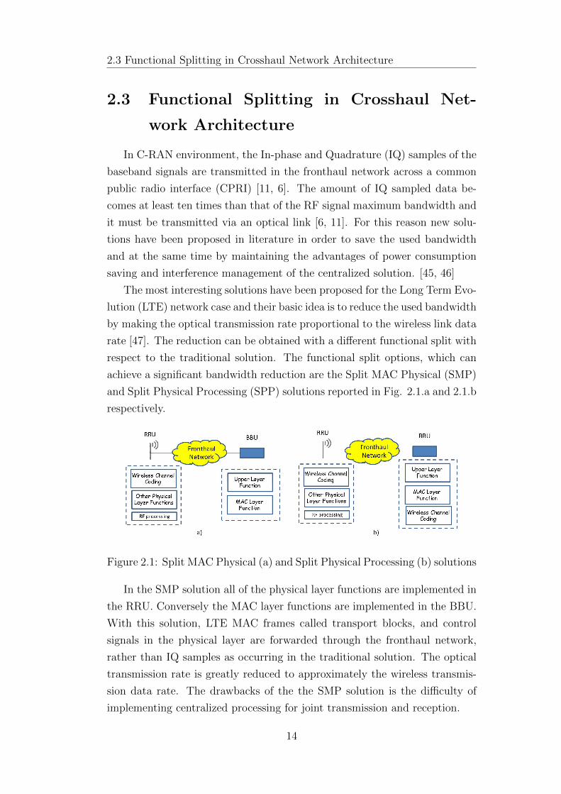
achieve a significant bandwidth reduction are the Split MAC Physical (SMP)
and Split Physical Processing (SPP) solutions reported in Fig. 2.1.a and 2.1.b
respectively.
Figure 2.1: Split MAC Physical (a) and Split Physical Processing (b) solutions
In the SMP solution all of the physical layer functions are implemented in
the RRU. Conversely the MAC layer functions are implemented in the BBU.
With this solution, LTE MAC frames called transport blocks, and control
signals in the physical layer are forwarded through the fronthaul network,
rather than IQ samples as occurring in the traditional solution. The optical
transmission rate is greatly reduced to approximately the wireless transmis-
sion data rate. The drawbacks of the the SMP solution is the difficulty of
implementing centralized processing for joint transmission and reception.
14

2.4 Evolution of Optical Transport Networks
In the SPP solution, the wireless channel coding is migrated towards the
BBU while the others physical layer functions as modulation and Multiple
Input Multiple Output (MIMO) are implemented in the RRU. This solution
allows the inter-cell interference management and the required optical link
capacity can be reduced to nearly that of the SMP solution and it depends
on the wireless transmission coding rate.
2.4 Evolution of Optical Transport Networks
Transport networks are migrating towards a simplified architecture basi-
cally composed of three layers [48, 49, 50]:
i) the Multi-protocol Label Switching (MPLS) layer, which is the
connection-oriented packet technology able to harmonize IP with circuit-
based worlds;
ii) the Optical Transport Network (OTN) layer [51, 52, 53], needed to handle
simultaneously packet and circuit-based services, with the right granular-
ity, while providing a level of performance monitoring, network surveil-
lance and fault recovery operations similar to the one provided by the
Synchronous Digital Hierarchy (SDH) network;
iii) the Wavelength Division Multiplexing (WDM) layer allowing routing of
individual wavelengths carrying high capacity channels benefiting from
the huge transmission bandwidth of the optical fiber.
This simplified transport network layering came out to simultaneously
fulfill key requirements such as to migrate the network towards the all-IP
paradigm and to reduce complexity and costs associated to traditional trans-
port technology based on circuit-switching (SDH/SONET). As a result, all the
transport functions that were assigned to SDH/SONET are now distributed
across different layers, partly in the optical (OTN and WDM) and partly in
the packet (MPLS).
The introduction of OTN switching [54]-[55] was a topic largely debated,
and many operators came to the conclusion that its use is needed to aggregate,
with an efficient bandwidth utilization, packet service data flows (from router
client interfaces) at lower rate into WDM data flows at higher rates in order
to lower the cost per transported bit [56, 57, 58]. Possible applications of the
OTN switching is in metropolitan area networks to aggregate both fixed and
15
2.4 Evolution of Optical Transport Networks
mobile traffic in a ring or mesh network topology. In fact in such networks
an higher level of functionalities are required but keeping at the same time
the cost acceptably low. In such applications the advantages offered to the
operators by the proposed node are the possibility to bring up services dy-
namically, the support of enhanced network applications such as protection
and restoration [59] and the provision of an extra level of flexibility by the
OTN subwavelength multiplexing and switching. Another case where OTN
switch can be important is in those applications where tough requirements
on latency are given.
Regarding a generic node of the transport network, it will contain multiple
switching layers, according to the level of switching and granularity needed in
that specific node. The most generic case is represented by a node logically
composed of three stacked switches, handling data flows at different levels of
traffic aggregation, namely MPLS (LSP: label switching paths tunnels), OTN
(ODU: optical channel data unit tunnels), and WDM (wavelength channels).
The ODU channels, defined by the G.709 standard [60, 61, 62] carry traf-
fic at medium-high sub-wavelength granularity, are cross-connected by the
OTN switch, while wavelength channels, carrying higher order data flows,
are optical switched typically by a ROADM (reconfigurable optical add-drop
multiplexer) [63, 64, 65, 66]. The finest granularity is so handled by the MPLS
switch.
There could be different levels of integration of the different layers, at
either data plane, or control plane, or even management plane; but in any
the real benefit of packet-optical integration is to offload the job of packet
switch/routers (e.g. MPLS), by routing bypass traffic in each node down to
the optical layer (either OTN or WDM) so as to save a significant number of
switch/routers ports leading to relevant reduction of power consumption and
costs [67, 68, 69].
A new concept of switch architecture referred to as Integrated OTN/WDM
switch [56, 57] assumes an OTN switch having integrated WDM interfaces in
the same system chassis as the switching functionality. This results in the
convergence of the WDM and OTN transmission functionality into a single
system, and has the benefit of eliminating any need for short-reach intercon-
nections between separate WDM and OTN systems, while also reducing the
rack space and power consumption.
More recently, the development and widespread deployment of multichan-
nel Photonic Integrated Circuit (PIC) technology [70]-[71], that enables the
16
2.5 Optical Node Architecture Options
integration of all the optical functions required for WDM transmission into a
single device, has helped to address these OTN/WDM integration.
2.5 Optical Node Architecture Options
Several packet-optical node architectures have been developed and put on
the field, and many other have been proposed in literature [72, 73]. They
differs each other from different points of view: number of switching layers,
switching architectures at the different layers, and related technologies, degree
of integration etc. Without loosing generality, they can be basically classified
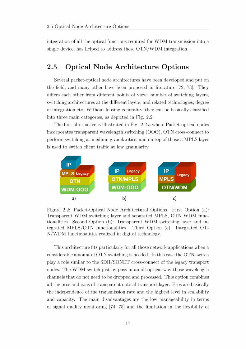
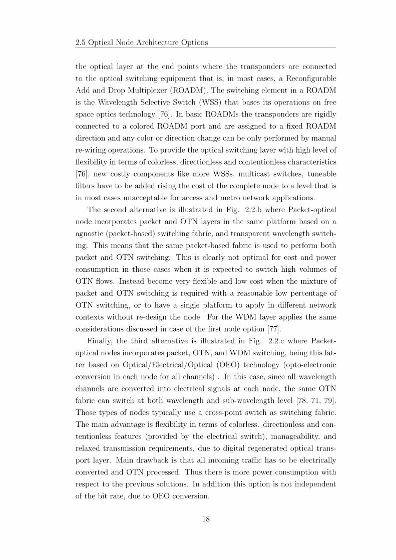
into three main categories, as depicted in Fig. 2.2.
The first alternative is illustrated in Fig. 2.2.a where Packet-optical nodes
incorporates transparent wavelength switching (OOO), OTN cross-connect to
perform switching at medium granularities, and on top of those a MPLS layer
is used to switch client traffic at low granularity.
WDM-OOO
OTN/MPLS
IP Legacy
OTN/WDM
MPLS
IPLegacy
WDM-OOO
OTN
MPLS Legacy
a)
b)
c)
IP
WDM-OOO
OTN/MPLS
IP Legacy
OTN/WDM
MPLS
IPLegacy
WDM-OOO
OTN
MPLS LegacyMPLS Legacy
a)
b)
c)
IP
WDM-OOO
OTN/MPLS
IP Legacy
OTN/WDM
MPLS
IPLegacy
WDM-OOO
OTN
MPLS Legacy
a)
b)
c)
IP
WDM-OOO
OTN/MPLS
IP Legacy
OTN/WDM
MPLS
IPLegacy
WDM-OOO
OTN
MPLS LegacyMPLS Legacy
a)
b)
c)
IP
WDM-OOO
OTN/MPLS
IP Legacy
OTN/WDM
MPLS
IPLegacy
WDM-OOO
OTN
MPLS Legacy
a)
b)
c)
IP
WDM-OOO
OTN/MPLS
IP Legacy
OTN/WDM
MPLS
IPLegacy
WDM-OOO
OTN
MPLS LegacyMPLS Legacy
a)
b)
c)
IP
a) b) c)
Figure 2.2: Packet-Optical Node Architectural Options. First Option (a):Transparent WDM switching layer and separated MPLS, OTN WDM func-tionalities. Second Option (b): Transparent WDM switching layer and in-tegrated MPLS/OTN functionalities. Third Option (c): Integrated OT-N/WDM functionalities realized in digital technology.
This architecture fits particularly for all those network applications when a
considerable amount of OTN switching is needed. In this case the OTN switch
play a role similar to the SDH/SONET cross-connect of the legacy transport
nodes. The WDM switch just by-pass in an all-optical way those wavelength
channels that do not need to be dropped and processed. This option combines
all the pros and cons of transparent optical transport layer. Pros are basically
the independence of the transmission rate and the highest level in scalability
and capacity. The main disadvantages are the low manageability in terms
of signal quality monitoring [74, 75] and the limitation in the flexibility of
17
2.5 Optical Node Architecture Options
the optical layer at the end points where the transponders are connected
to the optical switching equipment that is, in most cases, a Reconfigurable
Add and Drop Multiplexer (ROADM). The switching element in a ROADM
is the Wavelength Selective Switch (WSS) that bases its operations on free
space optics technology [76]. In basic ROADMs the transponders are rigidly
connected to a colored ROADM port and are assigned to a fixed ROADM
direction and any color or direction change can be only performed by manual
re-wiring operations. To provide the optical switching layer with high level of
flexibility in terms of colorless, directionless and contentionless characteristics
[76], new costly components like more WSSs, multicast switches, tuneable
filters have to be added rising the cost of the complete node to a level that is
in most cases unacceptable for access and metro network applications.
The second alternative is illustrated in Fig. 2.2.b where Packet-optical
node incorporates packet and OTN layers in the same platform based on a
agnostic (packet-based) switching fabric, and transparent wavelength switch-
ing. This means that the same packet-based fabric is used to perform both
packet and OTN switching. This is clearly not optimal for cost and power
consumption in those cases when it is expected to switch high volumes of
OTN flows. Instead become very flexible and low cost when the mixture of
packet and OTN switching is required with a reasonable low percentage of
OTN switching, or to have a single platform to apply in different network
contexts without re-design the node. For the WDM layer applies the same
considerations discussed in case of the first node option [77].
Finally, the third alternative is illustrated in Fig. 2.2.c where Packet-
optical nodes incorporates packet, OTN, and WDM switching, being this lat-
ter based on Optical/Electrical/Optical (OEO) technology (opto-electronic
conversion in each node for all channels) . In this case, since all wavelength
channels are converted into electrical signals at each node, the same OTN
fabric can switch at both wavelength and sub-wavelength level [78, 71, 79].
Those types of nodes typically use a cross-point switch as switching fabric.
The main advantage is flexibility in terms of colorless. directionless and con-
tentionless features (provided by the electrical switch), manageability, and
relaxed transmission requirements, due to digital regenerated optical trans-
port layer. Main drawback is that all incoming traffic has to be electrically
converted and OTN processed. Thus there is more power consumption with
respect to the previous solutions. In addition this option is not independent
of the bit rate, due to OEO conversion.
18

2.5 Optical Node Architecture Options
The first two categories are based on traditional transparent optical trans-
port, whose switches make use of all-optical costly devices such as wavelength
selective switches (WSS). Wavelength Selective Switches have reached the de-
velopment maturity and a cost reduction has become difficult due to the many
internal free-space optics parts to be aligned with high precision during the
assembly, and due to the hermetic and thermally compensated package re-
quired. In those cases the optical layer is essentially an analogue layer that
suffers from transmission impairments accumulation along the transmission
span. In addition they do not allow any real integration at HW level being
completely different technologies.
Differently, the third category is based on digital optical transport ap-
proach, which basically means to reconvert optical signal at each node and
to switch them in the electrical domain as any other digital electrical layer
with the consequence that a new opportunity come out: the possibility to
further integrate the WDM and the OTN switching layers, since they share
transceivers and cross-point switches, in order to further lower cost and energy
consumption.
The solutions proposed in [70] are based on strictly non-blocking high-
capacity OTN switches able to switch ODU sub-flows from low order (e.g.
ODU0) to high order (ODU3 ODU4). In those cases the OTN switches (or
cross-connect) are fully accessible, in the sense that each sub-flow, coming
from any input port can be routed to any output port at any ODU level.
This means that the architecture of the OTN switches are quite complex,
includes big switch fabrics, and thus are quite costly and energy consuming.
To reduce the switching fabric complexity, it is proposed the structure of
a scalable core switch [14, 80] composed of low capacity OTN switches and
one high capacity space switching fabric. It has shown [14] how the switching
architecture can be implemented by means of low cost market devices, in par-
ticular 12×12 OTN switches of 120Gbps capacity [1] and 144×144 crosspoints
of 1.44Tbps capacity [2].
A simplified integrated OTN/WDM switching architecture equipped with
reduced number of OTN switches has been also proposed in [81] where it has
shown how the introduction of OTN switches assignment policies can lead
to a remarkable reduction in number of OTN switches used. The analytical
evaluation of the blocking probability of the proposed integrated OTN/WDM
switches [14] shows how the blocking can be much high in some traffic scenario.
Its impact on the network blocking probability has been only marginally in-
19
2.5 Optical Node Architecture Options
vestigated [82] in the case of very simple routing strategies.
To reduce the blocking, in [83] it is proposed a more general integrated OT-
N/WDM switching architecture that can be provided with a spatial speedup
able to improve the blocking performance. Obviously the introduction of this
speedup increases the switch complexity and, in this case, the objective be-
comes to find the right trade-off between blocking degradation and complexity
increase. The impact of the switch blocking on the network performance in
static and dynamic traffic scenario has been investigated. Furthermore, it is
formulated the switch resource assignment and routing problem as an Integer
Linear Problem (ILP) and, to evaluate the blocking performance for large
networks and in static traffic scenario, an efficient heuristic has been intro-
duced. Finally the network blocking probability has been be evaluated by
simulation in dynamic traffic scenario.
20

Chapter 3
OTN/WDM Integrated
Switching Architecture
The introduction of Optical Transport Network (OTN) switching tech-
nology in metropolitan networks enables an efficient wavelength bandwidth
utilization and reduces the number of wavelengths, leading to reduced net-
work costs. It has been shown [83] that the use of integrated OTN/WDM
switch architecture is cost effective because it reduces the number of short-
reach client interfaces and the rack space compared to an architecture that
uses a reconfigurable optical adddrop multiplexer and a separate standalone
OTN switch or one that uses back-to-back muxponder connections to per-
form manual grooming. As seen in the Chapter 2, an integrated WDM-OTN
switch that allows for significantly lower complexity and cost at the price of
relaxing the non-blocking ideal performance requirements normally required
to such a kind of switch has been proposed [14].
This chapter treats the investigation of the impact that the switch blocking
has on the network performance in static and dynamic scenario for different
metropolitan networks. The routing problem in the integrated OTN/WDM
network as an Integer Linear Problem has been formulated in Section 3.2
and an efficient heuristic to evaluate the blocking performance in static traf-
fic scenario has been developed in Section 3.3. The Section 3.4 shows how
no blocking degradation occurs in a case study of different metropolitan net-
works. In particular it shows that the degradation of 2-3 orders of magnitude
in blocking probability occurring under dynamic traffic scenario can be miti-
gated with the introduction of a spatial speedup of value 1.5.
Furthermore a low complexity and integrated OTN/WDM switching ar-
22
3.1 OTN/WDM Integrated Switching Node
chitecture for metropolitan networks has been proposed in Section 3.5. This
switch is scalable and composed by small capacity OTN switches and one
space switch. The architecture reduces the number of OTN switches with
respect to other solutions proposed in literature with the consequence of op-
timizing the used OTN switching resources and the complexity of the space
switch. To study the impact on the blocking performance of the reduced
number of OTN switches, an Integer Linear Problem that models the rout-
ing and switch resource assignment problem in a network equipped with the
proposed switches has been introduced in Section 3.6. Being the problem
NP-hard, an heuristic is defined to evaluate the network request blocking in
static traffic scenario in Section 3.8. The obtained results show how a reduc-
tion in OTN switches as small as 50% can be reached when the percentage of
traffic needing sub-wavelength switching is 40%.
Next Section 3.1 reports the proposed integrated OTN/WDM switching
architecture and carries out a complexity analysis of the switching fabric as a
function of the spatial speedup. Finally conclusions and future research items
are illustrated in Section 3.10.
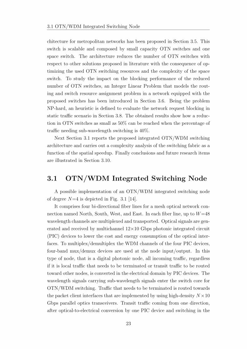
3.1 OTN/WDM Integrated Switching Node
A possible implementation of an OTN/WDM integrated switching node
of degree N=4 is depicted in Fig. 3.1 [14].
It comprises four bi-directional fiber lines for a mesh optical network con-
nection named North, South, West, and East. In each fiber line, up to W=48
wavelength channels are multiplexed and transported. Optical signals are gen-
erated and received by multichannel 12×10 Gbps photonic integrated circuit
(PIC) devices to lower the cost and energy consumption of the optical inter-
faces. To multiplex/demultiplex the WDM channels of the four PIC devices,
four-band mux/demux devices are used at the node input/output. In this
type of node, that is a digital photonic node, all incoming traffic, regardless
if it is local traffic that needs to be terminated or transit traffic to be routed
toward other nodes, is converted in the electrical domain by PIC devices. The
wavelength signals carrying sub-wavelength signals enter the switch core for
OTN/WDM switching. Traffic that needs to be terminated is routed towards
the packet client interfaces that are implemented by using high-density N×10
Gbps parallel optics transceivers. Transit traffic coming from one direction,
after optical-to-electrical conversion by one PIC device and switching in the
23
3.1 OTN/WDM Integrated Switching Node
W
N
S
ESWITCH CORE
Fiber Line
12x10G WDM PICNx10G parallel Optics Transceiver
Up to 48wavelengths
Band Mux/Demux
Figure 3.1: Implementation of an integrated OTN/WDM Switching Node
switch core, is routed toward another PIC connected to another direction for
electrical-to-optical conversion and transmission through the network.
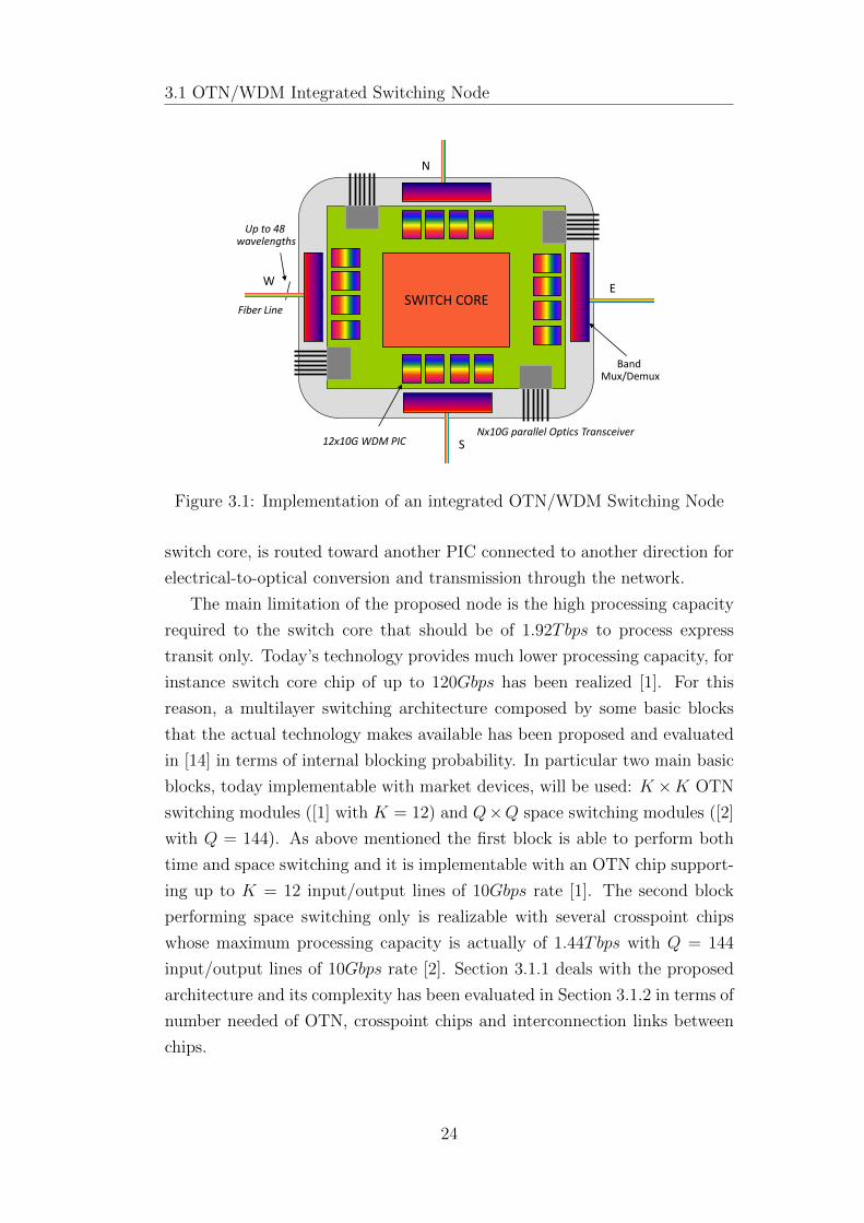
The main limitation of the proposed node is the high processing capacity
required to the switch core that should be of 1.92Tbps to process express
transit only. Today’s technology provides much lower processing capacity, for
instance switch core chip of up to 120Gbps has been realized [1]. For this
reason, a multilayer switching architecture composed by some basic blocks
that the actual technology makes available has been proposed and evaluated
in [14] in terms of internal blocking probability. In particular two main basic
blocks, today implementable with market devices, will be used: K ×K OTN
switching modules ([1] with K = 12) and Q×Q space switching modules ([2]
with Q = 144). As above mentioned the first block is able to perform both
time and space switching and it is implementable with an OTN chip support-
ing up to K = 12 input/output lines of 10Gbps rate [1]. The second block
performing space switching only is realizable with several crosspoint chips
whose maximum processing capacity is actually of 1.44Tbps with Q = 144
input/output lines of 10Gbps rate [2]. Section 3.1.1 deals with the proposed
architecture and its complexity has been evaluated in Section 3.1.2 in terms of
number needed of OTN, crosspoint chips and interconnection links between
chips.
24

3.1 OTN/WDM Integrated Switching Node
Parameter Description
N node degree
W number of wavelengths
fH H-ODU bit-rate
fL L-ODU bit-rate
F multiplexing ratio of fH to fL
CW wavelength capacity
K OTN switch size
H number of OTN switches per input/output line
T number of OTN switches in each ADD/DROPsection
CIL interstage link capacity
S spatial speedup
Q size of the basic switching module
Table 3.1: Switch Parameters
3.1.1 Switch Core Architecture
This section deals with the proposed switch core for hierarchical two-level
OTN transport architecture and able to switch two types of Optical Data
Units (ODU) referred to as higher order ODU (H-ODU) and lower order
ODU (L-ODU) respectively.
Next some switch parameters whose meaning is reported in Table 3.1 are
introduced.
The bit-rate of the H-ODU and L-ODU are denoted with fH and fL
respectively. furthermore the multiplexing ratio F of the H-ODU bit-rate to
the L-ODU bit-rate has been introduced. Here an important assumption is
that any input/output wavelength is characterized by a capacity CW equal
to fH and is hence able to carry either one H-ODU or up to F L-ODUs.
The switch can handle two typed of H-ODU. If an H-ODU needs only space
switching, it is referred to as “Direct” H-ODU (DH-ODU). Conversely if it
carries L-ODUs needing time switching it is referred to as “Switched” H-ODU
(SH-ODU).
The proposed switch core architecture, described in Fig. 3.2 [83], is com-
posed by three stages: K ×K OTN switching modules are placed in the first
25
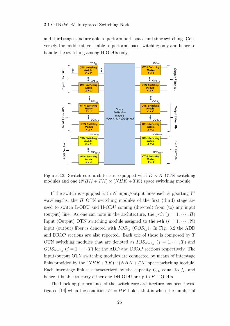
3.1 OTN/WDM Integrated Switching Node
and third stages and are able to perform both space and time switching. Con-
versely the middle stage is able to perform space switching only and hence to
handle the switching among H-ODUs only.
OTN SwitchingModuleK x K
IOS1,1
OTN SwitchingModuleK x K
IOS1,H
OTN SwitchingModuleK x K
IOSN,1
OTN SwitchingModuleK x K
IOSN,H
OTN SwitchingModuleK x K
OOS1,1
OTN SwitchingModuleK x K
OOS1,H
OTN SwitchingModuleK x K
OOSN,1
OTN SwitchingModuleK x K
OOSN,H
OTN SwitchingModuleK x K
IOSN+1,1
OTN SwitchingModuleK x K
IOSN+1,T
OTN SwitchingModuleK x K
OOSN+1,1
OTN SwitchingModuleK x K
OOSN+1,T
SpaceSwitching
Module(NHK+TK) x (NHK+TK)
Inpu
t F
iber
#1
Inpu
t F
iber
#N
AD
DS
ecti
on
Output F
iber
#1
Output F
iber
#N
DR
OP
Section
Figure 3.2: Switch core architecture equipped with K × K OTN switchingmodules and one (NHK + TK)× (NHK + TK) space switching module
If the switch is equipped with N input/output lines each supporting W
wavelengths, the H OTN switching modules of the first (third) stage are
used to switch L-ODU and H-ODU coming (directed) from (to) any input
(output) line. As one can note in the architecture, the j-th (j = 1, · · · , H)
Input (Output) OTN switching module assigned to the i-th (i = 1, · · · , N)
input (output) fiber is denoted with IOSi,j (OOSi,j). In Fig. 3.2 the ADD
and DROP sections are also reported. Each one of those is composed by T
OTN switching modules that are denoted as IOSN+1,j (j = 1, · · · , T ) and
OOSN+1,j (j = 1, · · · , T ) for the ADD and DROP sections respectively. The
input/output OTN switching modules are connected by means of interstage
links provided by the (NHK+TK)×(NHK+TK) space switching module.
Each interstage link is characterized by the capacity CIL equal to fH and
hence it is able to carry either one DH-ODU or up to F L-ODUs.
The blocking performance of the switch core architecture has been inves-
tigated [14] when the condition W = HK holds, that is when the number of
26
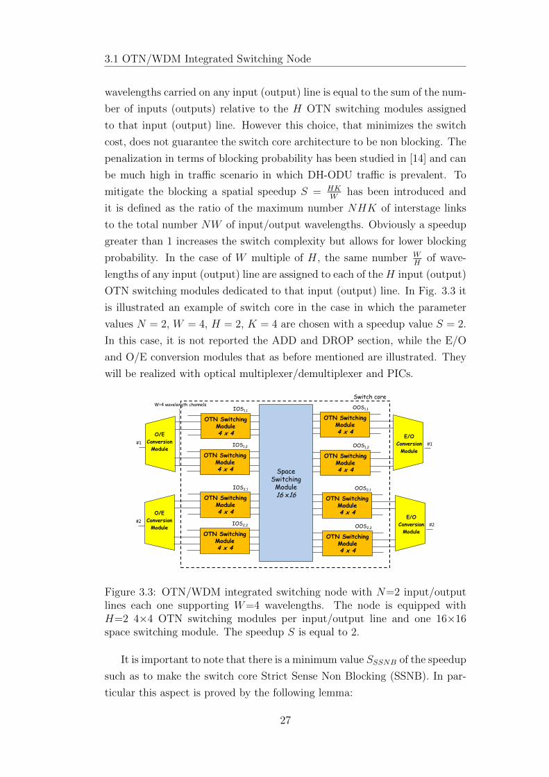
3.1 OTN/WDM Integrated Switching Node
wavelengths carried on any input (output) line is equal to the sum of the num-
ber of inputs (outputs) relative to the H OTN switching modules assigned
to that input (output) line. However this choice, that minimizes the switch
cost, does not guarantee the switch core architecture to be non blocking. The
penalization in terms of blocking probability has been studied in [14] and can
be much high in traffic scenario in which DH-ODU traffic is prevalent. To
mitigate the blocking a spatial speedup S = HKW
has been introduced and
it is defined as the ratio of the maximum number NHK of interstage links
to the total number NW of input/output wavelengths. Obviously a speedup
greater than 1 increases the switch complexity but allows for lower blocking
probability. In the case of W multiple of H, the same number WH
of wave-
lengths of any input (output) line are assigned to each of the H input (output)
OTN switching modules dedicated to that input (output) line. In Fig. 3.3 it
is illustrated an example of switch core in the case in which the parameter
values N = 2, W = 4, H = 2, K = 4 are chosen with a speedup value S = 2.
In this case, it is not reported the ADD and DROP section, while the E/O
and O/E conversion modules that as before mentioned are illustrated. They
will be realized with optical multiplexer/demultiplexer and PICs.
#1
O/E
Conversion
Module
W=4 wavelength channels
#1
E/O
Conversion
Module
OTN SwitchingModule4 x 4
IOS1,1
OTN SwitchingModule4 x 4
IOS1,2
#2
O/E
Conversion
Module
OTN SwitchingModule4 x 4
IOS2,1
OTN SwitchingModule4 x 4
IOS2,2
OTN SwitchingModule4 x 4
OOS1,1
OTN SwitchingModule4 x 4
OOS1,2
#2
E/O
Conversion
Module
OTN SwitchingModule4 x 4
OOS2,1
OTN SwitchingModule4 x 4
OOS2,2
SpaceSwitching
Module16 x16
Switch core
Figure 3.3: OTN/WDM integrated switching node with N=2 input/outputlines each one supporting W=4 wavelengths. The node is equipped withH=2 4×4 OTN switching modules per input/output line and one 16×16space switching module. The speedup S is equal to 2.
It is important to note that there is a minimum value SSSNB of the speedup
such as to make the switch core Strict Sense Non Blocking (SSNB). In par-
ticular this aspect is proved by the following lemma:
27

3.1 OTN/WDM Integrated Switching Node
Lemma 1. Under the constraint of W multiple of H, the proposed switch
core architecture is SSNB if the speedup S is greater than or equal to
SSSNB = d KbKFce
.
The proof of the lemma 1 is reported in Appendix A.1.
3.1.2 Switch Core Complexity Evaluation
The increase in speedup S can lead to better blocking performance and
even to a SSNB switch configuration when S is greater than or equal to
SSSNB. However the consequence is the complexity increase of the switch core
that we characterize with three indexes. The first complexity index nOTN is
characterized by the total number of K × K OTN switching modules used.
Because the space switching module is too big to be implemented with a single
chip, the second complexity index nSW is characterized by the total number of
Q×Q space switching modules needed to realize the space switching module
of the proposed switch core, being Q depending on the availability of market
devices. Finally the third complexity index nIL characterizes the number of
interconnection links between the switching modules.
Next it is reported the evaluation of the indexes nOTN , nSW and nIL as a
function of the speedup S when the ADD and DROP sections are neglected.
nOTN is simply given by 2HN and expressing H as a function of the speedup
S:
nOTN = 2SW
KN (3.1)
The parameter nSW is evaluated in the case in which the space switching
module has a three stages SSNB Clos network structure and characterizes the
least number of Q×Q switching modules needed to realize the space switch.
As preliminary result of the evaluation of nSW , the following lemma can be
enunciated:
Lemma 2. A U×U switching module with a three stages SSNB Clos network
structure can be realized with the least number NQ×Q of Q × Q (U > Q)
switching modules given by:
28
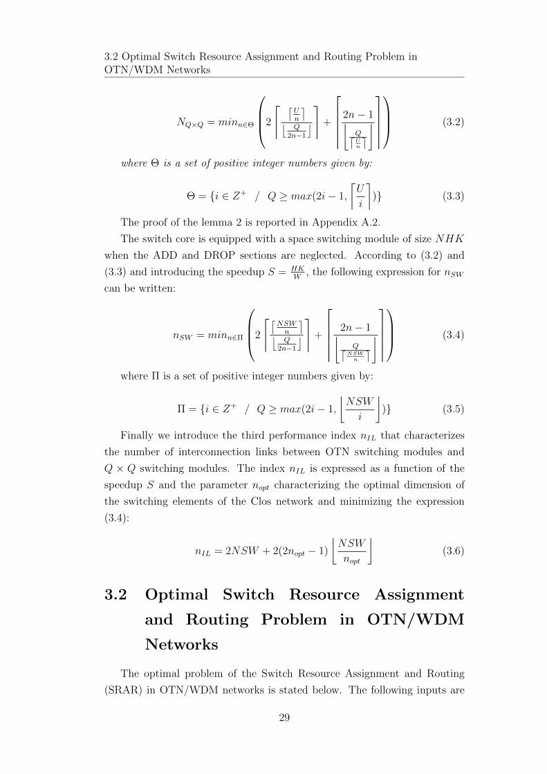
3.2 Optimal Switch Resource Assignment and Routing Problem inOTN/WDM Networks
NQ×Q = minn∈Θ
2
⌈ ⌈Un
⌉⌊Q
2n−1
⌋⌉+
2n− 1⌊
Q
dUn e
⌋ (3.2)
where Θ is a set of positive integer numbers given by:
Θ = i ∈ Z+ / Q ≥ max(2i− 1,
⌈U
i
⌉) (3.3)
The proof of the lemma 2 is reported in Appendix A.2.
The switch core is equipped with a space switching module of size NHK
when the ADD and DROP sections are neglected. According to (3.2) and
(3.3) and introducing the speedup S = HKW
, the following expression for nSW
can be written:
nSW = minn∈Π
2
⌈⌈NSWn
⌉⌊Q
2n−1
⌋ ⌉+
2n− 1⌊
Q
dNSWn e
⌋ (3.4)
where Π is a set of positive integer numbers given by:
Π = i ∈ Z+ / Q ≥ max(2i− 1,
⌊NSW
i
⌋) (3.5)
Finally we introduce the third performance index nIL that characterizes
the number of interconnection links between OTN switching modules and
Q × Q switching modules. The index nIL is expressed as a function of the
speedup S and the parameter nopt characterizing the optimal dimension of
the switching elements of the Clos network and minimizing the expression
(3.4):
nIL = 2NSW + 2(2nopt − 1)
⌊NSW
nopt
⌋(3.6)
3.2 Optimal Switch Resource Assignment
and Routing Problem in OTN/WDM
Networks
The optimal problem of the Switch Resource Assignment and Routing
(SRAR) in OTN/WDM networks is stated below. The following inputs are
29

3.2 Optimal Switch Resource Assignment and Routing Problem inOTN/WDM Networks
considered:
• G = (V , E): graph representing a physical topology where V is the
set of nodes and E is the set of links; the nodes correspond to the
OTN/WDM integrated switching nodes and the links correspond to
the fibers between switching nodes; the degree of the node v ∈ V is
assumed to be dv that is the corresponding switching node has dv express
input/output fibers; the network is composed by NV switching nodes,
each one equipped with K × K OTN switches and provided with a
speedup S.
• T : number of ADD/DROP OTN switches for each switching node;
• W : number of wavelength channels carried by each fiber where each
channel has the capacity of carrying either one H-ODU or up to F
L-ODUs;
• T DH = [tDHsd ], T L = [tLsd]: NV × NV traffic matrices for the DH-ODUs
and L-ODUs traffic offered between the network nodes respectively. In
particular tDHsd and tLsd denote the number of DH-ODUs and L-ODUs
offered between the nodes s ∈ V and d ∈ V ;
The goals are to determine:
• which interstage links are set up between the OTN switching modules
in the nodes v ∈ V ;
• where the accepted H-ODUs and L-ODUs traffic is routed in the OT-
N/WDM network.
The objective is to maximize the throughput given by total accepted band-
width traffic demand normalized to the bandwidth fL requested by one L-
ODU. In particular notice that the acceptance of one DH-ODU request and
one L-ODU request leads to a contribution of F and 1 respectively in the
normalized total accepted bandwidth traffic demand.
Next the optimization problem is described.
1) Notations and parameters
To give formally the ILP formulation, the unconnected graph G∗ =
(V∗, E∗) where V∗ and E∗ are the set of nodes and the links respectively
30
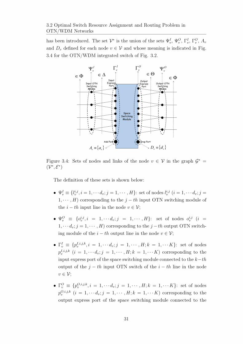
3.2 Optimal Switch Resource Assignment and Routing Problem inOTN/WDM Networks
has been introduced. The set V∗ is the union of the sets ΨIv, ΨO
v , ΓIv, ΓOv , Av
and Dv defined for each node v ∈ V and whose meaning is indicated in Fig.
3.4 for the OTN/WDM integrated switch of Fig. 3.2.
SpaceSwitching
Module
Input OTNSwitching
Module
Input Express
Port
Output Express
Port
Output OTNSwitching
Module
Add Port Drop Port
I
vΓ O
vΓI
vΨ O
vΨ
vvaA ≡
vvdD ≡
Θ∈∆∈Φ∈ Φ∈
Figure 3.4: Sets of nodes and links of the node v ∈ V in the graph G∗ =(V∗, E∗)
The definition of these sets is shown below:
• ΨIv ≡ li,jv , i = 1, · · · dv; j = 1, · · · , H: set of nodes li,jv (i = 1, · · · dv; j =
1, · · · , H) corresponding to the j − th input OTN switching module of
the i− th input line in the node v ∈ V ;
• ΨOv ≡ oi,jv , i = 1, · · · dv; j = 1, · · · , H: set of nodes oi,jv (i =
1, · · · dv; j = 1, · · · , H) corresponding to the j− th output OTN switch-
ing module of the i− th output line in the node v ∈ V ;
• ΓIv ≡ pI,i,j,kv , i = 1, · · · dv; j = 1, · · · , H; k = 1, · · ·K: set of nodes
pI,i,j,kv (i = 1, · · · dv; j = 1, · · · , H; k = 1, · · ·K) corresponding to the
input express port of the space switching module connected to the k−thoutput of the j − th input OTN switch of the i − th line in the node
v ∈ V ;
• ΓOv ≡ pO,i,j,kv , i = 1, · · · dv; j = 1, · · · , H; k = 1, · · ·K: set of nodes
pO,i,j,kv (i = 1, · · · dv; j = 1, · · · , H; k = 1, · · ·K) corresponding to the
output express port of the space switching module connected to the
31
3.2 Optimal Switch Resource Assignment and Routing Problem inOTN/WDM Networks
k − th input of the j − th output OTN switch of the i− th line in the
node v ∈ V ;
• Av ≡ av: set composed by the only node av that jointly represents
the ADD OTN switches and the ADD ports of the space switch of the
node v ∈ V ;
• Dv ≡ dv: set composed by the only node dv that jointly represents
the DROP OTN switches and the DROP ports of the space switch of
the node v ∈ V ;
The set E∗ is composed by the following three sets of links:
• Φ: set of links (oiv ,jv , liu,ju ) ((v, u) ∈ E ; j = 1, · · ·H) where the nodes
v and u are adjacent in G and the corresponding switching nodes are
interconnected with a fiber by the iv − th output line of the node v to
the iu − th input line of the node u;
• ∆: set of links (li,jv , pI,i,j,kv ) (v ∈ V ; i = 1, · · · dv; j = 1, · · · , H; k =
1, · · ·K) connecting nodes corresponding to input OTN switches and
input express ports;
• Θ: set of links (pO,i,j,kv , oi,jv ) (v ∈ V ; i = 1, · · · dv; j = 1, · · · , H; k =
1, · · ·K) connecting nodes corresponding to output express ports and
output OTN switches.
Furthermore for each node w ∈ V∗ the sets Ω(−)w and Ω
(+)w of the predeces-
sor and successor nodes respectively have been introduced. Thus it is possible
to write:
Ω(−)w = t ∈ V∗ / (w, t) ∈ E∗
Ω(+)w = t ∈ V∗ / (t, w) ∈ E∗
2) Optimization variables
• Sy,ts,d ∈ 0, 1 (s, d ∈ V ; y ∈ DH,L; t ∈ 1..tysd): the variable assumes
the value 1 if the t − th y-ODU offered between the nodes s and d is
successfully carried; otherwise it assumes the value 0;
32
3.2 Optimal Switch Resource Assignment and Routing Problem inOTN/WDM Networks
• λw,u,y,ts,d ∈ 0, 1 (s, d ∈ V ; (w, u) ∈ E∗; y ∈ DH,L, t ∈ 1..tysd): the
variable assumes the value 1 if the t − th y-ODU offered between the
nodes s and d is carried on the link (w, u); otherwise it assumes the
value 0;
• xvw,u ∈ 0, 1 (v ∈ V ;w ∈ ΓIv ∪ Av;u ∈ ΓOv ∪Dv): the variable assumes
the value 1 if the ports of the space switch corresponding to the nodes
w and u are interconnected by an interstage link.
3) Objective function
The objective is to maximize the throughput given by total accepted band-
width traffic demand normalized to the bandwidth fL requested by one L-
ODU:
Maximize :∑s,d∈V
tLs,d∑t=1
SL,ts,d + F∑s,d∈V
tDHs,d∑t=1
SDH,ts,d (3.7)
4) Constraints
Constraints are introduced to ensure that from an input and output ex-
press port of any space switch is activated only an interstage link. Conversely
up to a maximum of KT interstage links can be activated from/to the AD-
D/DROP sections. These constraints can be expressed as follows:
∑u∈ΓO
v ∪Dv
xvw,u ≤ 1 v ∈ V w ∈ ΓIv (3.8)
∑w∈ΓI
v∪Av
xvw,u ≤ 1 v ∈ V u ∈ ΓOv (3.9)
∑u∈ΓO
v ∪Dv
xvw,u ≤ KT v ∈ V w = av (3.10)
∑w∈ΓI
v∪Av
xvw,u ≤ KT v ∈ V u = dv (3.11)
For the t-th y-ODU (y ∈ DH,L; t ∈ [1..tysv]) offered between the nodes
s, v ∈ V , flow conservation constraints in every node w ∈ V∗ are introduced.
The constraints may not be respected only in the ADD and DROP nodes as
and dv where the total flow is equal to 1 and -1 respectively if the y-ODU is
successfully carried; otherwise is equal to 0. We can write:
33

3.2 Optimal Switch Resource Assignment and Routing Problem inOTN/WDM Networks
∑u∈Ω
(−)w
λu,w,y,ts,v −∑
u∈Ω(+)w
λw,u,y,ts,v =
−Sy,ts,v if w = as
Sy,ts,v if w = dv
0 otherwise
(3.12)
Further constraints are considered in order to guarantee that the traffic
routed on any link (w, u) ∈ E∗ in smaller than or equal to the link transport
capacity normalized to the bandwidth fL of one L-ODU. This capacity equals
F for the links (w, u) ∈ ∆ ∪ Θ that interconnect nodes corresponding to
input/output OTN switches and output/input express ports. In the case of
links (w, u) ∈ Φ interconnecting nodes corresponding to output OTN switch
and input OTN switch, the capacity equals the sum of the capacities provided
by the wavelength channels interconnecting them, that is KFS
. Finally another
constraint that limits to F the normalized capacity of any activated interstage
link has been added. In particular, it can be simply written as follow:
∑s,d∈V
tLs,d∑t=1
λw,u.L,ts,d + F∑s,d∈V
tDHs,d∑t=1
λw,u,DH,ts,d ≤ CL (3.13)
where CL is given by:
CL =
F if (w, u) ∈ ∆ ∪Θ
KFS
if (w, u) ∈ Φ
Fxvw,u if v ∈ V ;w ∈ ΓIv;u ∈ ΓOv ∪Dv
Fxvw,u if v ∈ V ;w ∈ ΓIv ∪ Av;u ∈ ΓOv
(3.14)
This section is concluded with a computational complexity analysis. If
we assume that only DH-ODUs are offered to the network and strict sense
non blocking switching nodes are used, the studied SRAR problem becomes
the Routing and Wavelength Assignment (RWA) optimization problem with
wavelength conversion. Because it is well known the RWA problem is NP-
complete [84], we can conclude that the SRAR problem is NP-complete too.
As the number of variables and equations increases exponentially with the
size of network, the speedup of the switch and the number of wavelengths on
each fiber, the ILP formulation will allow us to provide results only in the
case of small networks. In the next section an heuristic is introduced in order
to evaluate the performance of the proposed switch node architecture in large
34

3.3 Maximizing Shortest Path Traffic (MSPT) Heuristic
networks.
3.3 Maximizing Shortest Path Traffic
(MSPT) Heuristic
The Maximizing Shortest Path Traffic (MSPT) heuristic attempts in the
initial phase (Phase-1) to route the traffic on the shortest paths of the network
by carrying on each of them either one DH-ODU or F L-ODUs. If there is not
enough resources to carry all of the traffic on the shortest paths, the MSPT
heuristic will try to carry in the successive phase (Phase-2) the remaining
traffic on alternative paths. The main steps of the heuristic are illustrated in
Algorithm 1.
In the initialization phase the graph Gaux = (Vaux, Eaux) is built up (line 2)
where Vaux = V∗ and Eaux is obtained from E∗ with the addition of all of the
possible interstage links that connect input express and add ports to output
express and drop ports in any switching node. For instance the interstage
links added to the switching node with the representation in Fig. 3.5.a is
illustrated in Fig. 3.5.b.
SpaceSwitchingModule
a1
a2
b1
b2
b3
b4
b5
c1
c2
c3
c4
c5
d1
d2
SpaceSwitchingModule
a1
a2
b1
b2
b3
b4
b5
c1
c2
c3
c4
c5
d1
d2
SpaceSwitchingModule
a1
a2
b1
b2
b3
b4
b5
c1
c2
c3
c4
c5
d1
d2
a) b)
c)
Figure 3.5: Sets of nodes and links of a node v ∈ V in the graph G∗ = (V∗, E∗)(a); insertion of the interstage links in the graph G∗ = (V∗, E∗) (b); deletion oflinks after that the least cost path crossing the nodes a1,b1,c2,d1 is evaluatedby the MSPT heuristic.
35

3.3 Maximizing Shortest Path Traffic (MSPT) Heuristic
Algorithm 1 Maximizing Shortest Path Traffic (MSPT) Heuris-tic1: /*Initialization*/2: build up the auxiliary graph Gaux = (Vaux, Eaux)3: for s, u ∈ V do4: tDH,rsu = tDHsu ,tL,rsu = tLsu, ttot,rsu = tDH,rsu + FtL,rsu5: end for6: /*Phase-1. Routing of the DH-ODUs and the L-ODUs on the short-
est paths of Gaux*/7: label the links of Eaux with weight 18: evaluate in the graph Gaux the lengths csu (s, u ∈ V) between the nodes
as, du ∈ Vaux9: insert into the list L in decreasing order the values ttot,rsu (s, u ∈ V) greater
than or equal to F10: while L 6= do11: extract the first value ttot,rwz in the list L12: evaluate the least cost path Pw,z in Gaux and its length c(Pw,z)13: if (Pw,z exists) & &(c(Pw,z) = cwz) then14: remove the links of Gaux on the path Pw,z that become fully occupied15: remove the not admissible interstages links from Gaux16: /*Update the traffic demands to be routed*/17: ttot,rwz =ttot,rwz -F18: if ttot,rwz ≥ F then19: insert the value ttot,rwz into the list L20: end if21: if one DH-ODU is routed then22: tDH,rwz =tDH,rwz -123: else24: tL,rwz =tL,rwz − F25: end if26: end if27: end while28: /*Phase-2. Routing of the DH-ODUs and the L-ODUs on the alter-
native paths of Gaux*/29: for y ∈ DH,L do30: insert into the list Ly in decreasing order the values ty,rsu (s, u ∈ V) greater
than or equal to 131: label the links in Gaux with weights equal to the available link capacity in
terms of y-ODU the link can accept and deleting the links with no capacity32: while Ly 6= do33: extract the first value ty,rwz in the list Ly34: evaluate the least cost path Pw,z in Gaux35: if Pw,z exists then36: update in Gaux the weight of the links of Pw,z37: remove the full links of Gaux38: remove the not admissible interstages links from Gaux39: /*Update the traffic demands to be routed*/40: ty,rwz=ty,rwz -141: if ty,rwz ≥ 0 then42: insert the value ty,rwz into the list Ly43: end if44: end if45: end while46: end for
36
3.3 Maximizing Shortest Path Traffic (MSPT) Heuristic
In the initialization phase the variables tDH,rsu ,tL,rsu and ttot,rsu (s, u ∈ V) are
also initialized (line 4). They store during the execution of the MSPT heuristic
the number of DH-ODUs, L-ODUs and the normalized total bandwidth traffic
demand to be still routed respectively. At the beginning of the Phase-1 the
links in Eaux are labeled with weight 1 (line 7) and the length of the shortest
path csu(s, u ∈ V) between the nodes as, du ∈ Vaux are evaluated (line 8).
The evaluation of csu is important because during the execution of the MSPT
heuristic some links could be removed by Gaux and the knowledge of csu allow
us to understand if a least cost path evaluated when some links are removed
is or not a shortest path in the initial auxiliary graph Gaux. The normalized
total bandwidth traffic demands ttot,rsu (s, u ∈ V) are stored in the list Laccording to a decreasing order (line 9). At each iteration of the Phase-1,
the MSPT heuristic tries to route either one DH-ODU or F L-ODUs, on the
shortest path between the nodes w, z ∈ V in which the higher normalized
total bandwidth traffic demand ttot,rwz (line 11) is remaining to be routed. In
particular the least cost path Pw,z between the nodes aw, dz ∈ V∗ is evaluated
(line 12) and if both it exists and its length c(Pw,z) equals cwz (line 13) the
traffic routing is successfully and the graph Gaux with the variables tDH,rwz ,tL,rwz
and ttot,rwz (w, z ∈ V) are updated (lines 14-24). The updating of the graph
Gauxconsists in deleting the links belonging to the shortest path Pw,z (line 14)
and becoming fully occupied. Besides the interstage links belonging to Pw,z,other interstage links have to be deleted (line 15) from Gaux. They are referred
to as not admissible interstage links and their deletion is needed to respect
the constraints expressed by the Eqs (3.8)-(3.11). These constraints establish
that when an interstage link is setup between an input and an output space
switch port of any switching node, no other interstage links (not admissible
interstage links) can be set up from these input and output ports. For instance
if the shortest path crossing the nodes a1, b1, c2, d1 in Fig. 3.5.b is evaluated,
the application of the MSPT heuristic leads to the deletion of the links (a1, b1),
(b1, c2), (c2, d1). Furthermore the use of the interstage link (b1, c2) prevents
from setting up other interstage links that have to be deleted, that is the
links (b1, c1), (b1, c3), (b1, c4), (b1, c5), (b2, c2), (b3, c2), (b4, c2), (b5, c2). The
representation of the switch core when the links are deleted is shown in Fig.
3.5.c. Any traffic demand ttot,rwz is not more inserted in the list L when either
a shortest path Pw,z is not available or when its value is smaller than F . The
condition of list L empty (line 10) guarantees the end of the Phase-1.
At the beginning of the Phase-2, the traffic demands tDH,rsu , tL,rsu (s, u ∈ V)
37

3.3 Maximizing Shortest Path Traffic (MSPT) Heuristic
of DH-ODUs and L-ODUs not routed in the Phase-1 are stored in the lists
LDH and LL in decreasing order (line 30) respectively. When the type y
(y ∈ DH,L) of traffic (DH-ODU and L-ODU) is handled, each link of the
graph Gaux is labeled with a weight denoting the available link capacity (line
31) given by the number of y-ODUs the link can accept. The links with
capacity equal to zero are deleted. The MSPT heuristic tries to route the
higher traffic demand ty,rwz (line 33) on the least cost path Pw,z (line 34) of
the graph Gaux. If this operation is successfully (line 35), the graph and the
variables are updated (line 36-40). The traffic demand ty,rwz is again inserted
in the list Ly only if it is greater than 0 (line 41-43). The Phase-2 ends when
both the lists Ly (y ∈ DH,L) are empty (line 32).
This section is concluded with a computational time complexity evaluation
of the MSPT heuristic. Before giving an expression of the complexity, the
following observations could be done:
i) the heavier operation of MSPT is the evaluation of least cost paths;
ii) in the worst case MSPT evaluates a number of least cost paths as many
times as the total sum Dtot =∑
s,v∈V (tDH,rsv + tL,rsv ) of the traffic demand;
iii) if a least cost path is evaluated in the graph Gaux = (Vaux, Eaux) by using
the Dijstra algorithm with binary heap implementation, its computa-
tional complexity is equal to O(LauxlogNaux) where Naux and Laux are
the number of nodes and links of Gaux;
iv) it is easy to prove that in the worst case occurring in the initial phase
the graph Gaux is composed by Naux = 4LESWK+1K
+ 2NV nodes and
Laux = 2LESW2K+1K
+ 2NV(dmaxSW )2 links, NV , LE being the number
of nodes and links of the network graph G = (V , E) and dmax being the
maximum node degree.
According to these remarks we can conclude that the computational time
complexity of the MSPT heuristic is
O(DtotSW (LE +NVd2maxSW )log(SWLE +NV))
.
38

3.4 Numerical Results for the Proposed Architecture
3.4 Numerical Results for the Proposed Ar-
chitecture
In the first part, this section deals with a complexity analysis of the inte-
grated OTN/WDM switching node versus the spatial speedup S. Then the
impact that the parameter S has on the network blocking performance in
static and dynamic traffic scenario will be evaluated.
In Table 3.2 some results on the hardware complexity as a function of the
speedup S of the proposed integrated OTN/WDM switch are reported. As
reference scenario, we can consider the case in which the DH-ODU and the L-
ODU carry fH=10 Gbs and fL = 1.25 Gbs flows corresponding to ODU-2 and
ODU-0 respectively of the OTN multiplexing hierarchical respectively [54].
This choice leads to a value of F equal to 8. In this evaluation, an integrated
OTN/WDM switch with N=4 Input/Output lines each one carrying W=48
wavelengths is considered. Obviously this analysis can be carried out for other
scenarios and can be easily extended to the case in which a number of OTN
hierarchical levels greater than two is considered. An important assumption
is about the availability of the following market devices needed to realize the
proposed switch core:
i) OTN switching modules of size K=12 [1] with OTN processing and
switching total capacity of 120 Gbps;
ii) space switching modules of size Q=144 with switching total capacity of
1.44 Tbps [2].
As said above, in Table 3.2 there are reported the values of the complexity
parameters nOTN , nSW and nIL introduced in Section 3.1.2 and denoting the
number of 12×12 OTN switches used, the number 144×144 space switching
modules and the number of interconnection links respectively. From the Table
3.2, where the values of nOTN , nSW and nIL are reported versus the speedup
S, we can observe how the realization of an SSNB (S=SSSNB=12 according to
lemma 1) switch needs the use of many components that makes it unfeasible.
In particular it would be needed nOTN=384 12×12 OTN switches, nSW=99
144×144 space switching modules and nIL=13568 interconnection links. The
complexity may be dramatically dropped if the speedup S is lowered from
S=12 (SSNB case) to S=1.5. That would lead to the use of nOTN=48 12 ×12 OTN switches, nSW=9 144 × 144 space switching modules and nIL=976
39

3.4 Numerical Results for the Proposed Architecture
S nOTN nSW nIL
1 32 7 9601.5 48 9 14402 64 15 20483 96 23 31684 128 31 43526 192 47 6624
12 (SSNB) 384 99 13568
Table 3.2: Evaluation of the complexity indexes nOTN , nSW and nIL as afunction of the spatial speedup S. The switch parameters are N=4, W=48,F=8. DH-ODU and L-ODU carrying 10 Gbps and 1.25 Gbps flows respec-tively are considered. The basic blocks of the integrated OTN/WDM switchare 12 × 12 OTN switching modules at 120 Gbps [1] and 144 × 144 spaceswitching modules at 1.44 Tbps [2].
interconnection links with a reduction of 87.5%, 90.9% and 92.9% for each
type of network element respectively. Obviously it is important to study
the impact that the reduction in speedup S has on the network blocking
performance. For this reason the blocking performance results in static and
dynamic traffic scenarios will be shown in Section 3.4.1 and 3.4.2 respectively.
3.4.1 Blocking Performance in Static Traffic Scenario
In this section, the blocking performance is evaluated when the following
static traffic model is used to generate the traffic matrices T DH = [tDHsd ] and
T L = [tLsd] that report the number of DH-ODUs and L-ODUs offered between
each couple of nodes s, v ∈ V .
The traffic model is characterized by the following two parameters:
• Ao,sn: the total offered bandwidth traffic demand normalized to the
total network capacity; we have
Ao,sn =A0,s
Ctot
where Ao,s is the total offered bandwidth traffic demand and Ctot is
the total network capacity; because each wavelength is provided with a
capacity equal to fH we have Ctot=WLfH , L and W being the number
of network fibers and the number of wavelengths carried in any fiber
respectively;
40
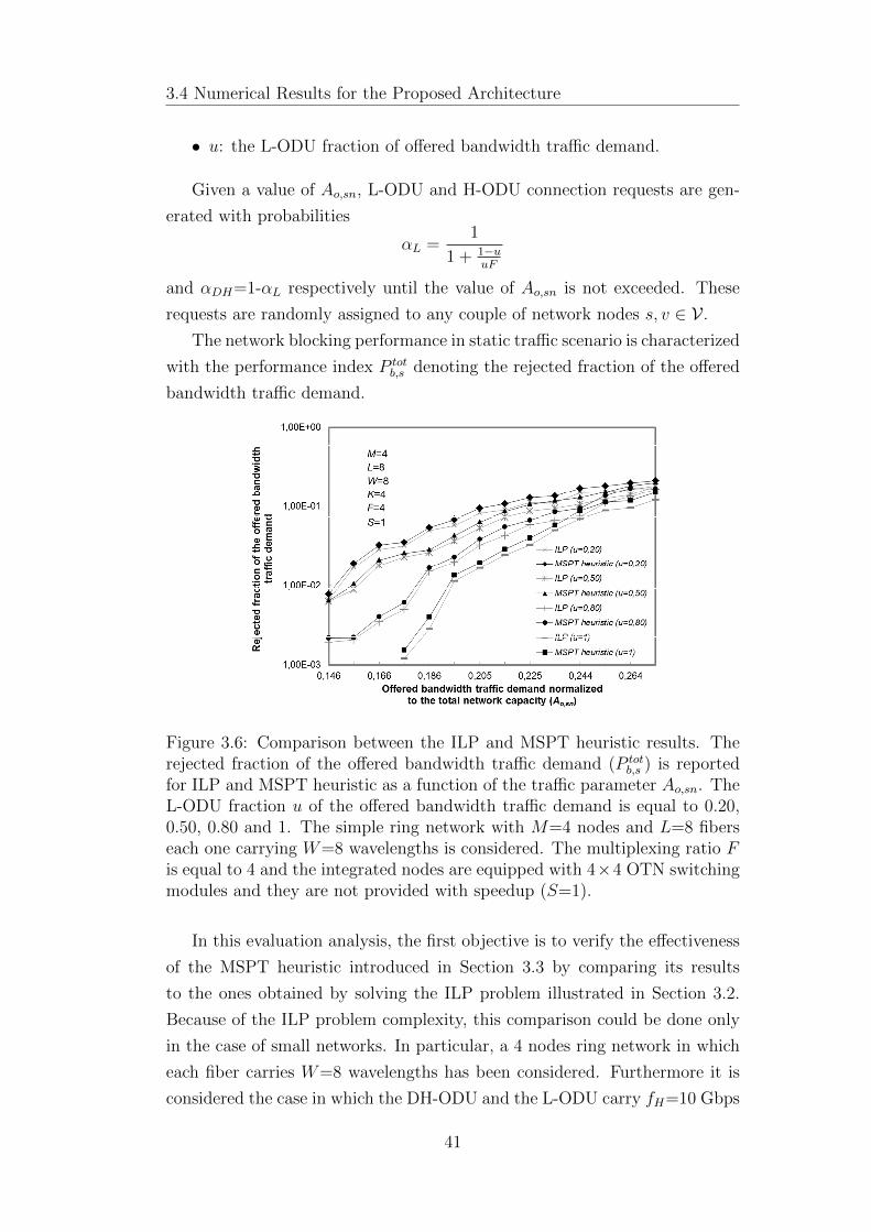
3.4 Numerical Results for the Proposed Architecture
• u: the L-ODU fraction of offered bandwidth traffic demand.
Given a value of Ao,sn, L-ODU and H-ODU connection requests are gen-
erated with probabilities
αL =1
1 + 1−uuF
and αDH=1-αL respectively until the value of Ao,sn is not exceeded. These
requests are randomly assigned to any couple of network nodes s, v ∈ V .
The network blocking performance in static traffic scenario is characterized
with the performance index P totb,s denoting the rejected fraction of the offered
bandwidth traffic demand.
Figure 3.6: Comparison between the ILP and MSPT heuristic results. Therejected fraction of the offered bandwidth traffic demand (P tot
b,s ) is reportedfor ILP and MSPT heuristic as a function of the traffic parameter Ao,sn. TheL-ODU fraction u of the offered bandwidth traffic demand is equal to 0.20,0.50, 0.80 and 1. The simple ring network with M=4 nodes and L=8 fiberseach one carrying W=8 wavelengths is considered. The multiplexing ratio Fis equal to 4 and the integrated nodes are equipped with 4×4 OTN switchingmodules and they are not provided with speedup (S=1).
In this evaluation analysis, the first objective is to verify the effectiveness
of the MSPT heuristic introduced in Section 3.3 by comparing its results
to the ones obtained by solving the ILP problem illustrated in Section 3.2.
Because of the ILP problem complexity, this comparison could be done only
in the case of small networks. In particular, a 4 nodes ring network in which
each fiber carries W=8 wavelengths has been considered. Furthermore it is
considered the case in which the DH-ODU and the L-ODU carry fH=10 Gbps
41
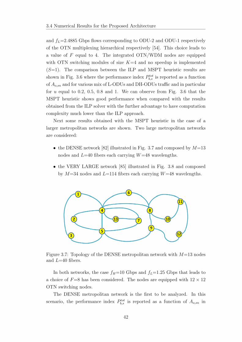
3.4 Numerical Results for the Proposed Architecture
and fL=2.4885 Gbps flows corresponding to ODU-2 and ODU-1 respectively
of the OTN multiplexing hierarchical respectively [54]. This choice leads to
a value of F equal to 4. The integrated OTN/WDM nodes are equipped
with OTN switching modules of size K=4 and no speedup is implemented
(S=1). The comparison between the ILP and MSPT heuristic results are
shown in Fig. 3.6 where the performance index P totb,s is reported as a function
of Ao,sn and for various mix of L-ODUs and DH-ODUs traffic and in particular
for u equal to 0.2, 0.5, 0.8 and 1. We can observe from Fig. 3.6 that the
MSPT heuristic shows good performance when compared with the results
obtained from the ILP solver with the further advantage to have computation
complexity much lower than the ILP approach.
Next some results obtained with the MSPT heuristic in the case of a
larger metropolitan networks are shown. Two large metropolitan networks
are considered:
• the DENSE network [82] illustrated in Fig. 3.7 and composed by M=13
nodes and L=40 fibers each carrying W=48 wavelengths.
• the VERY LARGE network [85] illustrated in Fig. 3.8 and composed
by M=34 nodes and L=114 fibers each carrying W=48 wavelengths.
Figure 3.7: Topology of the DENSE metropolitan network with M=13 nodesand L=40 fibers.
In both networks, the case fH=10 Gbps and fL=1.25 Gbps that leads to
a choice of F=8 has been considered. The nodes are equipped with 12 × 12
OTN switching nodes.
The DENSE metropolitan network is the first to be analyzed. In this
scenario, the performance index P totb,s is reported as a function of Ao,sn in
42

3.4 Numerical Results for the Proposed Architecture
Figure 3.8: Topology of the VERY LARGE metropolitan network with M=34nodes and L=114 fibers.
Figs 3.9-3.10 for speedup values S equal to 1, 1.5, 2, and 12 where S=12
corresponds to the SSNB switching node case. The traffic mix characterized
by u equal to 0.2 and 0.8 is considered in Fig. 3.9 while the results for u equal
to 0.5 and 1 are shown in Fig. 3.10. We can observe from Figs 3.9-3.10 that
even in the case in which the speedup is not implemented (S=1) performance
degradation does not occur and the same performance obtained with SSNB
(S=12) nodes are reached.
Considering the scenario with the metropolitan networks in Fig. 3.8, the
rejected fraction of the offered bandwidth traffic demand is reported in Fig.
3.11. In the VERY LARGE network, we can observe that when the speedup
is not implemented (S=1), performance degradation of more than one or-
der of magnitude occurs with respect to an SSNB switch. The performance
degradation may be mitigated by introducing a spatial speedup value S=1.5.
3.4.2 Blocking Performance in Dynamic Traffic Sce-
nario
The performance of the DENSE network of Fig. 3.7 with W=48 wave-
lengths carried on each fiber is investigated when the network is equipped
with the integrated OTN/WDM switching nodes and in the case of dynamic
traffic scenario. The first assumption is that the connection requests for
carrying L-ODU and DH-ODU are presented with exponentially distributed
inter-arrival times. The connection duration is also exponentially distributed
and we assume that L-ODU and DH-ODU carry flows at fL=1.25 Gbps and
43

3.4 Numerical Results for the Proposed Architecture
Figure 3.9: The rejected fraction of the offered bandwidth traffic demand(P tot
b,s ) is reported for the MSPT heuristic as a function of the traffic parameterAo,sn. The L-ODU fraction u of the offered bandwidth traffic demand is equalto 0.20 and 0.80. The network parameter values are M=13, L=40, W=48,F=8. The integrated OTN/WDM nodes are equipped with 12 × 12 OTNswitching modules and provided with speedup S varying from 1 to 12. Thecase S=12 corresponds to the case of SSNB switching nodes.
Figure 3.10: The rejected fraction of the offered bandwidth traffic demand(P tot
b,s ) is reported for the MSPT heuristic as a function of the traffic parameterAo,sn. The L-ODU fraction u of the offered bandwidth traffic demand is equalto 0.50 and 1. The network parameter values are M=13, L=40, W=48, F=8.The integrated OTN/WDM nodes are equipped with 12× 12 OTN switchingmodules and provided with speedup S varying from 1 to 12. The case S=12corresponds to the case of SSNB switching nodes.
44

3.4 Numerical Results for the Proposed Architecture
Figure 3.11: The rejected fraction of the offered bandwidth traffic demand(P tot
b,s ) is reported for the MSPT heuristic as a function of the normalizedoffered bandwidth traffic intensity Ao,sn. The L-ODU fraction u of the offeredbandwidth traffic demand is equal to 0.20 and 0.80. The network parametervalues are M=34, L=114, W=48, F=8. The integrated OTN/WDM nodesare equipped with 12×12 OTN switching modules and provided with speedupS varying from 1 to 12. The case S=12 corresponds to the case of SSNBswitching nodes.
fH=10 Gbps respectively that leads to a multiplexing ratio F=8.
Furthermore it is assumed uniformly distributed traffic between the net-
work nodes and denote with λL and λDH the connection request inter-arrival
rates of L-ODU and DH-ODU respectively. The same connection rate µ=1 is
assumed for L-ODU and and DH-ODU.
The offered traffic is characterized with the parameter
Ao,dn = N(N − 1)FλDH + λLWLF
that indicates the offered bandwidth traffic intensity normalized to the
total network capacity. In the dynamic traffic scenario, the expression could
be written for the L-ODU fraction of the offered bandwidth traffic as follow:
u =λL
λL + FλDH
The adopted routing policy is based on the use of two auxiliary graphs
GDHaux and GLaux for routing of L-ODU and DH-ODU respectively. The graphs
are constructed as described in Section 3.3 and are updated all of times in
which a connection carrying L-ODU or DH-ODU is set up or torn down.
45
3.4 Numerical Results for the Proposed Architecture
At any instant the graph GDHaux (GLaux) contains all of the links in which the
allocation of one DH-ODU (L-ODU) is permitted. Each link is labeled with a
weight denoting the number of DH-ODUs (L-ODUs) that the link can accept.
When a DH-ODU (L-ODU) connection request arrives, the least cost path
is evaluated in GDHaux (GLaux) and if it exists then the weights of the graphs
are updated and the links not able to accept at least one DH-ODU (L-ODU)
are deleted from the graph GDHaux (GLaux). As described in Section 3.3, the not
admissible interstage links are also removed. When a connection is torn down,
the graphs weights are updated and the links becoming newly available are
inserted as well as the admissible interstage links.
In the analysis reported in this section, three performance indexes charac-
terizing the network blocking under dynamic traffic scenario are introduced.
The first index is the rejected bandwidth ratio P totb,d defined as the bandwidth
blocking probability and characterizing the rejected fraction of the offered
bandwidth traffic. The second (third) index is the L-ODU (DH-ODU) con-
nection blocking probability PLb,d (PDH
b,d ) defined as the ratio of the number
of rejected L-ODU (DH-ODU) connection requests to the number of offered
L-ODU (DH-ODDU) connection requests. The indexes P totb,d , PL
b,d and PDHb,d
are evaluated as a function of Ao,dn for speedup values S equal to 1, 1.5, 2,
12 where the case S = SSSNB = 12 corresponds to the use of a Strict Sense
Non Blocking (SSNB) switch according to the Lemma-1 of Section 3.1.2.
The curves of P totb,d , PDH
b,d and PLb,d evaluated with the analysis of the DENSE
network are reported in Figs 3.12-3.14 for u=0.2 and u=0.8. Conversely the
ones for u=0.5 and u=1 for the same network are illustrated in Figs 3.15-
3.17. We can observe from Figs 3.12 and 3.15 a degradation of the band-
width blocking probability P totb,d when no speedup is implemented (S=1). For
instance when Ao,dn=0.091 and u=0.5, the bandwidth blocking probability
P totb,d equals 1.44 · 10−6 and 1.80 · 10−4 for the SSNB (S=12) and S=1 cases
with a worsening of two orders of magnitude. We can notice from Fig. 3.13
that the internal blocking of the switch and the lack of speedup lead espe-
cially a degradation in terms of the DH-ODU connection blocking probability.
In this case PDHb,d reaches values of 1.50 · 10−6 and 3.59 · 10−4 in the SSNB
and S=1 cases respectively and for Ao,dn=0.091 and u=0.5. Notice that the
higher reject rate of the DH-ODU connection requests leads to the possibil-
ity of accepting more L-ODU connection requests. That justifies why PLb,d is
lower in the case S=1 as shown in Figs 3.14 and 3.17.
Finally we can notice how a spatial speedup S equal to 1.5 leads to a lack
46
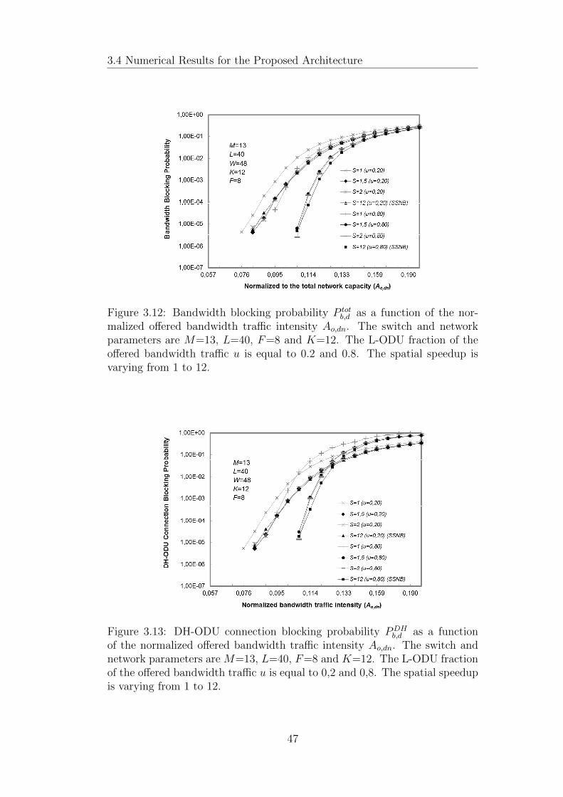
3.4 Numerical Results for the Proposed Architecture
Figure 3.12: Bandwidth blocking probability P totb,d as a function of the nor-
malized offered bandwidth traffic intensity Ao,dn. The switch and networkparameters are M=13, L=40, F=8 and K=12. The L-ODU fraction of theoffered bandwidth traffic u is equal to 0.2 and 0.8. The spatial speedup isvarying from 1 to 12.
Figure 3.13: DH-ODU connection blocking probability PDHb,d as a function
of the normalized offered bandwidth traffic intensity Ao,dn. The switch andnetwork parameters are M=13, L=40, F=8 and K=12. The L-ODU fractionof the offered bandwidth traffic u is equal to 0,2 and 0,8. The spatial speedupis varying from 1 to 12.
47

3.4 Numerical Results for the Proposed Architecture
Figure 3.14: L-ODU connection blocking probability PLb,d as a function of the
normalized offered bandwidth traffic intensity Ao,dn. The switch and networkparameters are M=13, L=40, F=8 and K=12. The L-ODU fraction of theoffered bandwidth traffic u is equal to 0.2 and 0.8. The spatial speedup isvarying from 1 to 12.
Figure 3.15: Bandwidth blocking probability P totb,d as a function of the nor-
malized offered bandwidth traffic intensity Ao,dn. The switch and networkparameters are M=13, L=40, F=8 and K=12. The L-ODU fraction of theoffered bandwidth traffic u is equal to 0.5 and 1, whereas the spatial speedupis varying from 1 to 12.
48

3.4 Numerical Results for the Proposed Architecture
Figure 3.16: DH-ODU connection blocking probability PDHb,d as a function
of the normalized offered bandwidth traffic intensity Ao,dn. The switch andnetwork parameters are M=13, L=40, F=8 and K=12. The L-ODU fractionof the offered bandwidth traffic u is equal to 0.5, whereas the spatial speedupis varying from 1 to 12.
Figure 3.17: L-ODU connection blocking probability PLb,d as a function of the
normalized offered bandwidth traffic intensity Ao,dn. The switch and networkparameters are M=13, L=40, F=8 and K=12. The L-ODU fraction of theoffered bandwidth traffic u is equal to 0.5 and 1. The spatial speedup isvarying from 1 to 12.
49
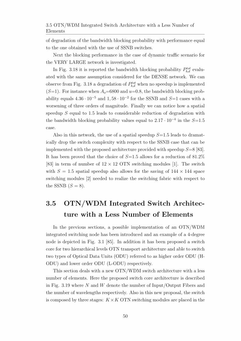
3.5 OTN/WDM Integrated Switch Architecture with a Less Number ofElements
of degradation of the bandwidth blocking probability with performance equal
to the one obtained with the use of SSNB switches.
Next the blocking performance in the case of dynamic traffic scenario for
the VERY LARGE network is investigated.
In Fig. 3.18 it is reported the bandwidth blocking probability P totb,d evalu-
ated with the same assumption considered for the DENSE network. We can
observe from Fig. 3.18 a degradation of P totb,d when no speedup is implemented
(S=1). For instance when Ao=6800 and u=0.8, the bandwidth blocking prob-
ability equals 4.36 · 10−5 and 1, 58 · 10−2 for the SSNB and S=1 cases with a
worsening of three orders of magnitude. Finally we can notice how a spatial
speedup S equal to 1.5 leads to considerable reduction of degradation with
the bandwidth blocking probability values equal to 2.17 · 10−4 in the S=1.5
case.
Also in this network, the use of a spatial speedup S=1.5 leads to dramat-
ically drop the switch complexity with respect to the SSNB case that can be
implemented with the proposed architecture provided with speedup S=8 [83].
It has been proved that the choice of S=1.5 allows for a reduction of 81.2%
[83] in term of number of 12 × 12 OTN switching modules [1]. The switch
with S = 1.5 spatial speedup also allows for the saving of 144 × 144 space
switching modules [2] needed to realize the switching fabric with respect to
the SSNB (S = 8).
3.5 OTN/WDM Integrated Switch Architec-
ture with a Less Number of Elements
In the previous sections, a possible implementation of an OTN/WDM
integrated switching node has been introduced and an example of a 4-degree
node is depicted in Fig. 3.1 [85]. In addition it has been proposed a switch
core for two hierarchical levels OTN transport architecture and able to switch
two types of Optical Data Units (ODU) referred to as higher order ODU (H-
ODU) and lower order ODU (L-ODU) respectively.
This section deals with a new OTN/WDM switch architecture with a less
number of elements. Here the proposed switch core architecture is described
in Fig. 3.19 where N and W denote the number of Input/Output Fibers and
the number of wavelengths respectively. Also in this new proposal, the switch
is composed by three stages: K×K OTN switching modules are placed in the
50
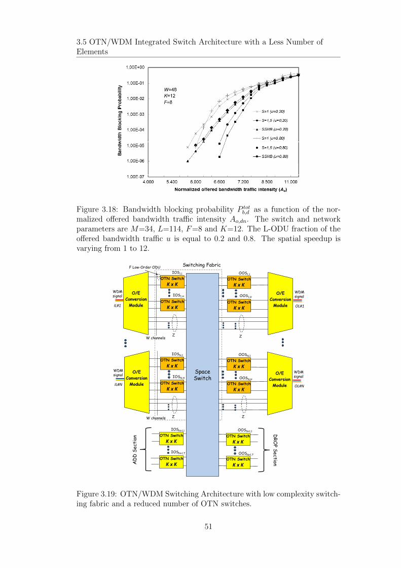
3.5 OTN/WDM Integrated Switch Architecture with a Less Number ofElements
Figure 3.18: Bandwidth blocking probability P totb,d as a function of the nor-
malized offered bandwidth traffic intensity Ao,dn. The switch and networkparameters are M=34, L=114, F=8 and K=12. The L-ODU fraction of theoffered bandwidth traffic u is equal to 0.2 and 0.8. The spatial speedup isvarying from 1 to 12.
IOS1,1
W channels
OTN Switch
K x K
OTN Switch
K x K
IOS1,H
IL#1
WDMsignal
Z
IOSN,1
W channels
OTN Switch
K x K
OTN Switch
K x K
IOSN,H
OL#N
WDMsignal
Z
Switching FabricF Low-Order ODU
OOS1,1
OTN Switch
K x K
OTN Switch
K x K
OOS1,H
Z
OOSN,1
OTN Switch
K x K
OTN Switch
K x K
Z
OOSN,H
IOSN+1,1
OTN Switch
K x K
OTN Switch
K x K
IOSN+1,T
OOSN+1,1
OTN Switch
K x K
OTN Switch
K x K
OOSN+1,T
SpaceSwitch
AD
DS
ect
ion
DR
OP
Section
O/E
Conversion
Module
IL#N
WDMsignal
O/E
Conversion
Module
O/E
Conversion
Module
OL#1
WDMsignal
O/E
Conversion
Module
Figure 3.19: OTN/WDM Switching Architecture with low complexity switch-ing fabric and a reduced number of OTN switches.
51

3.5 OTN/WDM Integrated Switch Architecture with a Less Number ofElements
first and third stages and are able to perform both space and time switching.
Conversely the middle stage is able to perform space switching only and hence
to handle the switching among H-ODUs only.
In each of the N input/output lines, a number H of OTN switches are
used while there are Z out of W wavelengths carried in each input/output line
for which OTN switching is not allowed. We assume that the OTN switching
modules of the first (third) stage are used to switch L-ODU and H-ODU
coming (directed) from (to) any input (output) line.
In Fig. 3.19 it is also reported the ADD and DROP sections each one
composed by T OTN switching modules. The input/output OTN switching
modules are connected by means of interstage links provided by the (NHK+
NZ + TK)× (NHK +NZ + TK) space switching module.
The blocking performance of the switch core architecture has been inves-
tigated [81] when the condition W−ZH
= K holds that is the used number of
inputs (outputs) of each input (output) OTN switch is equal to its size K.
However this choice, that minimizes the switch cost, does not guarantee the
switch core architecture to be non blocking. The penalization in terms of
blocking probability has been studied in [81] and can be much high in some
traffic scenario. To mitigate the blocking, it has been introduced a spatial
speedup
S =K
W−ZH
that is defined as the ratio of the OTN switch size to the used number of
inputs (outputs) of each input (output) OTN switch.
Obviously a speedup S greater than 1 increases the switch complexity but
allows for lower blocking probability. In the case of W −Z multiple of H, we
adopt the strategy of assigning the same number W−ZH
of wavelengths of any
input (output) line to each of the H input (output) OTN switching modules
dedicated to that input (output) line.
In Fig. 3.20 an example of proposed switching architecture is illustrated
in the case in which the parameter values N = 2, W = 6, H = 1, K = 4 are
chosen with a speedup value S = 2.
In this case, it has neglected to report the ADD and DROP sections while
we have illustrated the E/O and O/E conversion modules that as before
mentioned will be realized with optical multiplexer/demultiplexer and PICs.
52
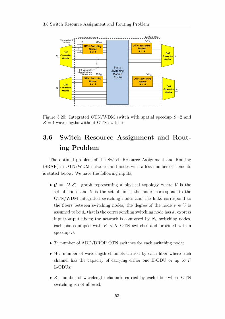
3.6 Switch Resource Assignment and Routing Problem
#1
O/E
Conversion
Module
W=6 wavelengthchannels
#1
E/O
Conversion
Module
OTN SwitchingModule4 x 4
IOS1,1
#2
O/E
Conversion
Module
OTN SwitchingModule4 x 4
IOS2,1
OTN SwitchingModule4 x 4
OOS1,1
#2
E/O
Conversion
Module
OTN SwitchingModule4 x 4
OOS2,1
SpaceSwitching
Module16 x16
Switch core
Z=6 wavelengthchannels without
OTN switches
(W-Z)/H=2 used inputs
Figure 3.20: Integrated OTN/WDM switch with spatial speedup S=2 andZ = 4 wavelengths without OTN switches.
3.6 Switch Resource Assignment and Rout-
ing Problem
The optimal problem of the Switch Resource Assignment and Routing
(SRAR) in OTN/WDM networks and nodes with a less number of elements
is stated below. We have the following inputs:
• G = (V , E): graph representing a physical topology where V is the
set of nodes and E is the set of links; the nodes correspond to the
OTN/WDM integrated switching nodes and the links correspond to
the fibers between switching nodes; the degree of the node v ∈ V is
assumed to be dv that is the corresponding switching node has dv express
input/output fibers; the network is composed by NV switching nodes,
each one equipped with K × K OTN switches and provided with a
speedup S.
• T : number of ADD/DROP OTN switches for each switching node;
• W : number of wavelength channels carried by each fiber where each
channel has the capacity of carrying either one H-ODU or up to F
L-ODUs;
• Z: number of wavelength channels carried by each fiber where OTN
switching is not allowed;
53

3.6 Switch Resource Assignment and Routing Problem
• T DH = [tDHsd ], T L = [tLsd]: NV × NV traffic matrices for the DH-ODUs
and L-ODUs traffic offered between the network nodes respectively. In
particular tDHsd and tLsd denote the number of DH-ODUs and L-ODUs
offered between the nodes s ∈ V and d ∈ V ;
Also in this problem like the one reported in Section 3.2, the goal is to
determine:
• where the accepted H-ODUs and L-ODUs traffic is routed in the OT-
N/WDM network;
• which interstage links are set up between the input and output ports of
the space switches of the nodes v ∈ V .
The objective is to maximize the throughput given by total accepted band-
width traffic demand normalized to the bandwidth fL requested by one L-
ODU. In particular notice that the acceptance of one DH-ODU request and
one L-ODU request leads to a contribution of F and 1 respectively in the
normalized total accepted bandwidth traffic demand.
1) Notation and parameters
To give formally the ILP formulation, the unconnected graph G∗ =
(V∗, E∗) is introduced where V∗ and E∗ are the set of nodes and the links re-
spectively. The set V∗ is the union of the sets ΨIv, ΨO
v , ΓI,OTNv , ΓI,Fv , ΓO,OTNv ,
ΓO,Fv , Av and Dv defined for each node v ∈ V and whose meaning is indicated
in Fig. 3.21 for the OTN/WDM integrated switch of Fig. 3.20.
In the following, the definition of these sets is provided:
• ΨIv ≡ li,jv , i = 1, · · · dv; j = 1, · · · , H: set of nodes li,jv (i = 1, · · · dv; j =
1, · · · , H) corresponding to the j − th input OTN switching module of
the i− th input line in the node v ∈ V ;
• ΨOv ≡ oi,jv , i = 1, · · · dv; j = 1, · · · , H: set of nodes oi,jv (i =
1, · · · dv; j = 1, · · · , H) corresponding to the j− th output OTN switch-
ing module of the i− th output line in the node v ∈ V ;
• ΓI,OTNv ≡ pI,OTN,i,j,kv , i = 1, · · · dv; j = 1, · · · , H; k = 1, · · ·K: set of
nodes pI,OTN,i,j,kv (i = 1, · · · dv; j = 1, · · · , H; k = 1, · · ·K) correspond-
ing to the input express port of the space switching module connected
to the k − th output of the j − th input OTN switch of the i− th line
in the node v ∈ V ;
54

3.6 Switch Resource Assignment and Routing Problem
SpaceSwitching
Module
Input OTNSwitching
Module
Input Express
Port Output Express
Port
Output OTNSwitching
Module
Add Port Drop Port
OTNI
v
,Γ OTNO
v
,ΓI
vΨ O
vΨ
vvaA ≡
vvdD ≡
Θ∈∆∈Φ∈ Φ∈
ξ∈
ξ∈
FI
v
,Γ FO
v
,Γ
Figure 3.21: Sets of nodes and links of the node v ∈ V in the graph G∗ =(V∗, E∗)
• ΓI,Fv ≡ pI,F,i,jv , i = 1, · · · dv; j = 1, · · · , Z: set of nodes pI,F,i,jv (i =
1, · · · dv; j = 1, · · · , Z) corresponding to the input express port of the
space switching module connected to the j−th wavelengths of the i−thinput line in the node v ∈ V in which OTN switch are absent;
• ΓO,OTNv ≡ pO,OTN,i,j,kv , i = 1, · · · dv; j = 1, · · · , H; k = 1, · · ·K: set of
nodes pO,OTN,i,j,kv (i = 1, · · · dv; j = 1, · · · , H; k = 1, · · ·K) correspond-
ing to the output express port of the space switching module connected
to the k − th input of the j − th output OTN switch of the i− th line
in the node v ∈ V ;
• ΓO,Fv ≡ pO,F,i,jv , i = 1, · · · dv; j = 1, · · · , Z: set of nodes pO,F,i,jv (i =
1, · · · dv; j = 1, · · · , H) corresponding to the output express port of the
space switching module connected to the j−th wavelengths of the i−thoutput line in the node v ∈ V in which OTN switches are absent;
• Av ≡ av: set composed by the only node av that jointly represents
the ADD OTN switches and the ADD ports of the space switch of the
node v ∈ V ;
• Dv ≡ dv: set composed by the only node dv that jointly represents
the DROP OTN switches and the DROP ports of the space switch of
the node v ∈ V ;
The set E∗ is composed by the following four sets of links:
55

3.6 Switch Resource Assignment and Routing Problem
• Φ: set of links (oiv ,jv , liu,ju ) ((v, u) ∈ E ; j = 1, · · ·H) where the nodes
v and u are adjacent in G and the corresponding switching nodes are
interconnected with a fiber by the iv − th output line of the node v to
the iu − th input line of the node u;
• ξ: set of links (pO,F,iv ,jv , pI,F,iu,ju ) ((v, u) ∈ E ; j = 1, · · ·Z) where the
nodes v and u are adjacent in G and the corresponding switching nodes
are interconnected with a fiber by the iv − th output line of the node v
to the iu − th input line of the node u;
• ∆: set of links (li,jv , pI,i,j,kv ) (v ∈ V ; i = 1, · · · dv; j = 1, · · · , H; k =
1, · · ·K) connecting nodes corresponding to input OTN switches and
input express ports;
• Θ: set of links (pO,i,j,kv , oi,jv ) (v ∈ V ; i = 1, · · · dv; j = 1, · · · , H; k =
1, · · ·K) connecting nodes corresponding to output express ports and
output OTN switches.
For each node w ∈ V∗ the sets Ω(−)w and Ω
(+)w of the predecessor and
successor nodes respectively have been introduced. thus we can write:
Ω(−)w = t ∈ V∗ / (t, w) ∈ E∗
Ω(+)w = t ∈ V∗ / (w, t) ∈ E∗
2) Optimization Variables
Next the variables of the optimization problem are reported:
• Sy,ts,d ∈ 0, 1 (s, d ∈ V ; y ∈ DH,L; t ∈ 1..tysd): the variable assumes
the value 1 if the t − th y-ODU offered between the nodes s and d is
successfully carried; otherwise it assumes the value 0;
• λw,u,y,ts,d ∈ 0, 1 (s, d ∈ V ; (w, u) ∈ E∗; y ∈ DH,L, t ∈ 1..tysd): the
variable assumes the value 1 if the t − th y-ODU offered between the
nodes s and d is carried on the link (w, u); otherwise it assumes the
value 0;
• xvw,u ∈ 0, 1 (v ∈ V ;w ∈ ΓI,OTNv ∪ ΓI,Fv ∪ Av;u ∈ ΓO,OTNv ∪ ΓO,Fv ∪Dv): the variable assumes the value 1 if the ports of the space switch
56
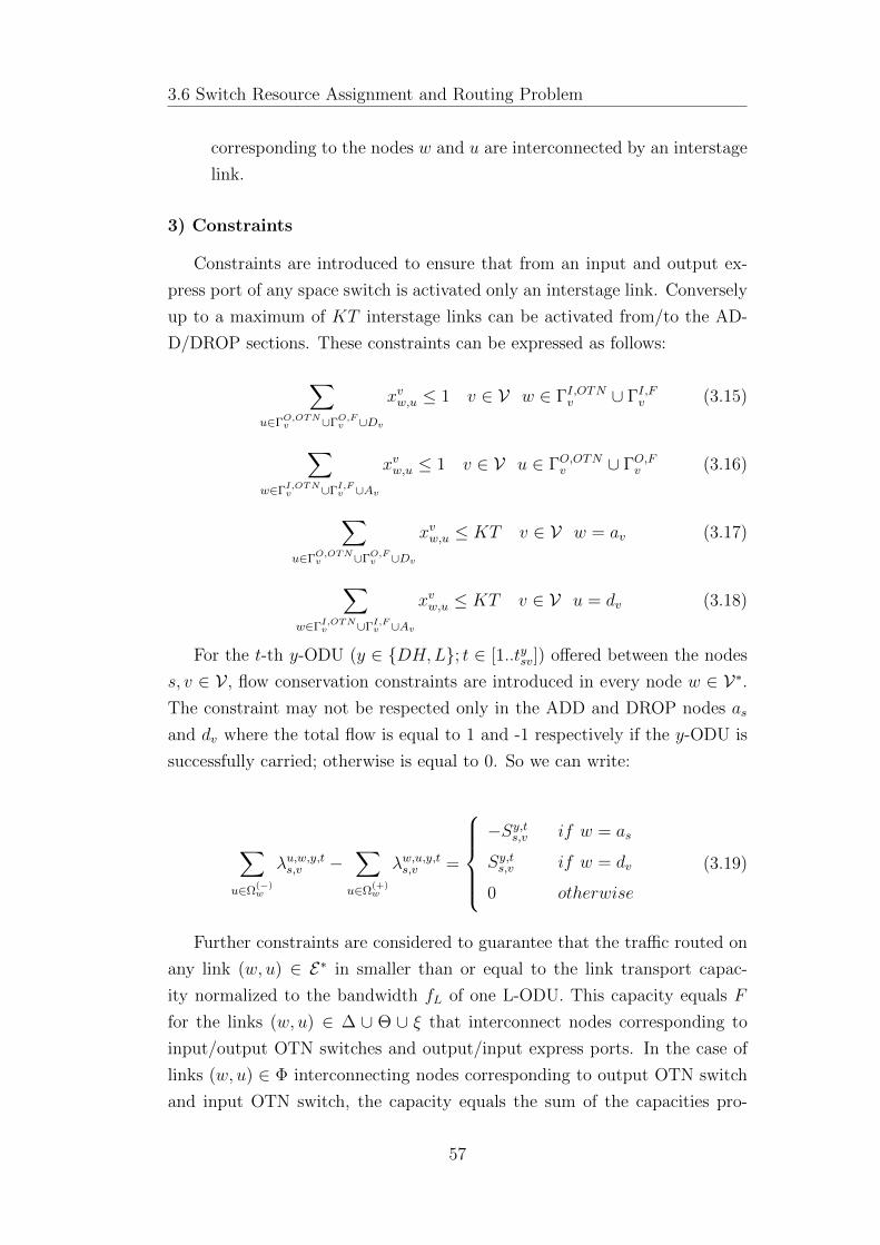
3.6 Switch Resource Assignment and Routing Problem
corresponding to the nodes w and u are interconnected by an interstage
link.
3) Constraints
Constraints are introduced to ensure that from an input and output ex-
press port of any space switch is activated only an interstage link. Conversely
up to a maximum of KT interstage links can be activated from/to the AD-
D/DROP sections. These constraints can be expressed as follows:
∑u∈ΓO,OTN
v ∪ΓO,Fv ∪Dv
xvw,u ≤ 1 v ∈ V w ∈ ΓI,OTNv ∪ ΓI,Fv (3.15)
∑w∈ΓI,OTN
v ∪ΓI,Fv ∪Av
xvw,u ≤ 1 v ∈ V u ∈ ΓO,OTNv ∪ ΓO,Fv (3.16)
∑u∈ΓO,OTN
v ∪ΓO,Fv ∪Dv
xvw,u ≤ KT v ∈ V w = av (3.17)
∑w∈ΓI,OTN
v ∪ΓI,Fv ∪Av
xvw,u ≤ KT v ∈ V u = dv (3.18)
For the t-th y-ODU (y ∈ DH,L; t ∈ [1..tysv]) offered between the nodes
s, v ∈ V , flow conservation constraints are introduced in every node w ∈ V∗.The constraint may not be respected only in the ADD and DROP nodes as
and dv where the total flow is equal to 1 and -1 respectively if the y-ODU is
successfully carried; otherwise is equal to 0. So we can write:
∑u∈Ω
(−)w
λu,w,y,ts,v −∑
u∈Ω(+)w
λw,u,y,ts,v =
−Sy,ts,v if w = as
Sy,ts,v if w = dv
0 otherwise
(3.19)
Further constraints are considered to guarantee that the traffic routed on
any link (w, u) ∈ E∗ in smaller than or equal to the link transport capac-
ity normalized to the bandwidth fL of one L-ODU. This capacity equals F
for the links (w, u) ∈ ∆ ∪ Θ ∪ ξ that interconnect nodes corresponding to
input/output OTN switches and output/input express ports. In the case of
links (w, u) ∈ Φ interconnecting nodes corresponding to output OTN switch
and input OTN switch, the capacity equals the sum of the capacities pro-
57
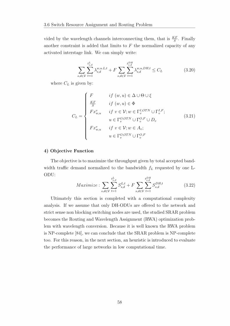
3.6 Switch Resource Assignment and Routing Problem
vided by the wavelength channels interconnecting them, that is KFS
. Finally
another constraint is added that limits to F the normalized capacity of any
activated interstage link. We can simply write:
∑s,d∈V
tLs,d∑t=1
λw,u.L,ts,d + F∑s,d∈V
tDHs,d∑t=1
λw,u,DH,ts,d ≤ CL (3.20)
where CL is given by:
CL =
F if (w, u) ∈ ∆ ∪Θ ∪ ξKFS
if (w, u) ∈ Φ
Fxvw,u if v ∈ V ;w ∈ ΓI,OTNv ∪ ΓI,Fv ;
u ∈ ΓO,OTNv ∪ ΓO,Fv ∪Dv
Fxvw,u if v ∈ V ;w ∈ Av;
u ∈ ΓO,OTNv ∪ ΓO,Fv
(3.21)
4) Objective Function
The objective is to maximize the throughput given by total accepted band-
width traffic demand normalized to the bandwidth fL requested by one L-
ODU:
Maximize :∑s,d∈V
tLs,d∑t=1
SL,ts,d + F∑s,d∈V
tDHs,d∑t=1
SDH,ts,d (3.22)
Ultimately this section is completed with a computational complexity
analysis. If we assume that only DH-ODUs are offered to the network and
strict sense non blocking switching nodes are used, the studied SRAR problem
becomes the Routing and Wavelength Assignment (RWA) optimization prob-
lem with wavelength conversion. Because it is well known the RWA problem
is NP-complete [84], we can conclude that the SRAR problem is NP-complete
too. For this reason, in the next section, an heuristic is introduced to evaluate
the performance of large networks in low computational time.
58
3.7 Minimizing OTN Switch Resource (MOSR) Heuristic
3.7 Minimizing OTN Switch Resource
(MOSR) Heuristic
In the case of integrated OTN/WDM switching architectures equipped
with the minimum number of OTN switches, it is very important to exploit
wavelengths that are not supported by OTN switches, assigning to each of
these either one DH-ODU or F L-ODUs. In the following in order to refer to
these ones, the most generic term “H-ODU” is used.
The Minimizing OTN Switch Resource (MOSR) heuristic, shown in Algo-
rithm 2, attempts in the first phase to route the traffic on the shortest paths
of the network by carrying on each of them one H-ODU. Moreover among
the available shortest paths, the one with minimum number of OTN switches
used is selected.
If there is not enough resources to carry all of the traffic on the shortest
paths, the MOSR heuristic will try to carry in Phase-2 the remaining traffic
on alternative paths.
Before the Phase-1, there is an initialization phase, not shown in Algo-
rithm 2, in which the auxiliary graph Gaux = (Vaux, Eaux) is built up, where
Vaux = V∗ and Eaux is obtained from E∗ with the addition of all of the possible
interstage links that connect input express and add ports to output express
and drop ports in any switching node.
The normalized total bandwidth traffic demands ttotsu=FtDHsu +tLsu (s, u ∈ V)
are stored in the list L1 according to a decreasing order (line 2). At each
iteration of the Phase-1, the MOSR heuristic tries to route either one DH-
ODU or F L-ODUs, on the shortest path between the nodes s∗, u∗ ∈ V in
which the higher normalized total bandwidth traffic demand ttots∗u∗ (line 4) is
remaining to be routed. The shortest path with minimum number of OTN
switches used is selected.
Any traffic demand ttots∗u∗ is not more inserted in the list L1 when either
a shortest path is not available or when its value is smaller than F . The
condition of list L1 empty (line 3) guarantees the end of the Phase-1. At the
beginning of the Phase-2, the traffic demands of DH-ODUs and L-ODUs not
routed in the first phase are stored in the lists LDH and LL in decreasing
order (line 12) respectively.
The MOSR heuristic tries to route the higher traffic demand on the path
with minimum number of links (line 15). The alternative path with minimum
59
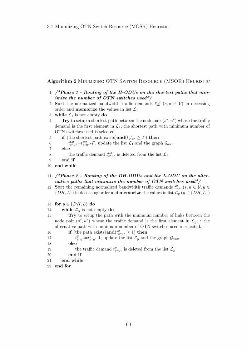
3.7 Minimizing OTN Switch Resource (MOSR) Heuristic
Algorithm 2 Minimizing OTN Switch Resource (MSOR) Heuristic
1: /*Phase 1 - Routing of the H-ODUs on the shortest paths that min-imize the number of OTN switches used*/
2: Sort the normalized bandwidth traffic demands ttotsu (s, u ∈ V) in deceasingorder and memorize the values in list L1
3: while L1 is not empty do4: Try to setup a shortest path between the node pair (s∗, u∗) whose the traffic
demand is the first element in L1; the shortest path with minimum number ofOTN switches used is selected.
5: if (the shortest path exists)and(ttots∗u∗ ≥ F ) then6: ttots∗u∗=ttots∗u∗-F , update the list L1 and the graph Gaux7: else8: the traffic demand ttots∗u∗ is deleted from the list L1
9: end if10: end while
11: /*Phase 2 - Routing of the DH-ODUs and the L-ODU on the alter-native paths that minimize the number of OTN switches used*/
12: Sort the remaining normalized bandwidth traffic demands tys,u (s, u ∈ V, y ∈DH,L) in deceasing order and memorize the values in list Ly (y ∈ DH,L)
13: for y ∈ DH,L do14: while Ly is not empty do15: Try to setup the path with the minimum number of links between the
node pair (s∗, u∗) whose the traffic demand is the first element in Ly; ; thealternative path with minimum number of OTN switches used is selected.
16: if (the path exists)and(tys∗u∗ ≥ 1) then17: tys∗u∗=tys∗u∗-1, update the list Ly and the graph Gaux18: else19: the traffic demand tys∗u∗ is deleted from the list Ly20: end if21: end while22: end for
60
3.8 Numerical Results for the Less Complex Architecture
number of OTN switches used is selected. If this operation is successfully, the
graph and the variables are updated (line 17). The Phase-2 ends when both
the lists Ly (y ∈ DH,L) are empty (line 14).
3.8 Numerical Results for the Less Complex
Architecture
Next this section deals with some results obtained with the MOSR heuris-
tic in the case of a larger metropolitan network illustrated in Fig. 3.8, that
is composed by M=34 nodes and L=114 fibers each carrying W=48 wave-
lengths.
The case fH=10 Gbs and fL=1.25 Gbs is considered, leading to a choice
of F=8. The nodes are equipped with 12× 12 OTN switching nodes.
The blocking performance has been evaluated when the following static
traffic model is used to generate the traffic matrices T DH = [tDHsd ] and T L =
[tLsd] that report the number of DH-ODUs and L-ODUs offered between each
couple of nodes s, v ∈ V .
The traffic model is characterized by the two parameters:
• Ao,sn that is defined as the total offered bandwidth traffic demand nor-
malized to the total network capacity; we have
Ao,sn =A0,s
Ctot
where Ao,s is the total offered bandwidth traffic demand and Ctot is
the total network capacity; because each wavelength is provided with a
capacity equal to fH we have Ctot=WLfH .
• u defined as the L-ODU fraction of offered bandwidth traffic demand.
Given a value of Ao,sn, L-ODU and H-ODU connection requests are gen-
erated with probabilities
uL =1
1 + 1−uuF
and uDH=1-αL respectively until the value of Ao,sn is not exceeded. These
requests are randomly assigned to any couple of network nodes s, v ∈ V .
The network blocking performance in static traffic scenario are character-
ized with the performance index P totb,s denoting the rejected fraction of the
offered bandwidth traffic demand.
61

3.8 Numerical Results for the Less Complex Architecture
Fig. 3.22 plots the performance index P totb,s as a function of u when
Ao,sn=0.57 and the network is equipped with integrated OTN/WDM opti-
cal switches provided with a spatial speedup S=1.5. The number H of OTN
switches per Input/Output Fiber (IF/OF) is varied from 1 to 6, where H=6
corresponds to the case in which all of wavelengths are equipped with OTN
switches.
Figure 3.22: The rejected fraction of the offered bandwidth traffic demand(P tot
b,s ) is reported for the MOSR heuristic as a function of the L-ODU fractionu of offered bandwidth traffic demand and when Ao,sn=0.57.
u nOTN αOTN nCP αCP
0.1 228 83.3% 250 18.83%0.2 456 66.7% 250 18.83%0.3 456 66.7% 250 18.83%0.4 684 50% 264 14.29%0.5 912 33.3% 264 14.29%0.6 1140 16.7% 306 0.64%
Table 3.3: Complexity indexes nOTN ,αOTN ,nCP and αCP as a function of theL-ODU fraction u of offered bandwidth traffic demand. The same parametervalues of Fig. 3.22 are chosen and the space switch are realized with 144×144crosspoints [2].
We can see from Fig. 3.22 that, increasing the value of u, the blocking
probability P totb,s decreases due to the reduced granularity of the offered traffic
bandwidth. For instance in the case H=6, we obtain values of P totb,s equal to
3.41 · 10−4 and 1.29 · 10−5 when the L-ODU fraction u of offered bandwidth
62

3.9 Further Analysis
traffic demand equal to 0.5 and 0.9 respectively. Furthermore, increasing the
value of u, we need to have an higher number of H and a greater space switch
complexity as a consequence in order to guarantees the same performance of
the case in which all of the wavelengths are provided with all of the OTN
switches (H=6). For instance we need H=2 and H=3 OTN switches per
IF/OF for u=0.3 and u=0.4 respectively in order to guarantee the minimum
blocking probability of the case H=6.
To characterize the complexity reduction that the proposed architecture
allows us to obtain with respect to the classical architecture using all of the
OTN switches when the same bandwidth blocking probability P totb,s is guar-
anteed, in Table 3.3 for u varying from 0.1 to 0.6 the following indexes are
reported:
• nOTN , total number of OTN switches used;
• αOTN , the percentage saving of OTN switches with respect to the case
in which all of the OTN switches ate used (H=6);
• nCP , total number of 144 × 144 crosspoints [2] needed to realize all of
the space switches;
• αCP , percentage saving of 144× 144 crosspoints [2] with respect to the
case H=6.
As a matter of example, in the case in which the L-ODU fraction u of
offered bandwidth traffic demand is equal to 0.4, only half (H=3) of OTN
switches per IF/OF can be used and saving of 50% and 14.29% of OTN
switches and 144× 144 crosspoints respectively are possible.
3.9 Further Analysis
In the previous sections, three-stages architecture for the OTN/WDM
integrated switch are proposed and evaluated. In Fig. 3.23 [14, 81], in order
to further reduce switch cost and power consumption, a new architecture with
only two stages is proposed and the performance of the blocking switching
fabric are investigated.
As said above, the architecture reported in Fig. 3.23, where N and W
denote the number of Input/Output Lines (IL/OL) and the number of wave-
lengths supported per each IL/OL respectively, is composed by two stages.
63
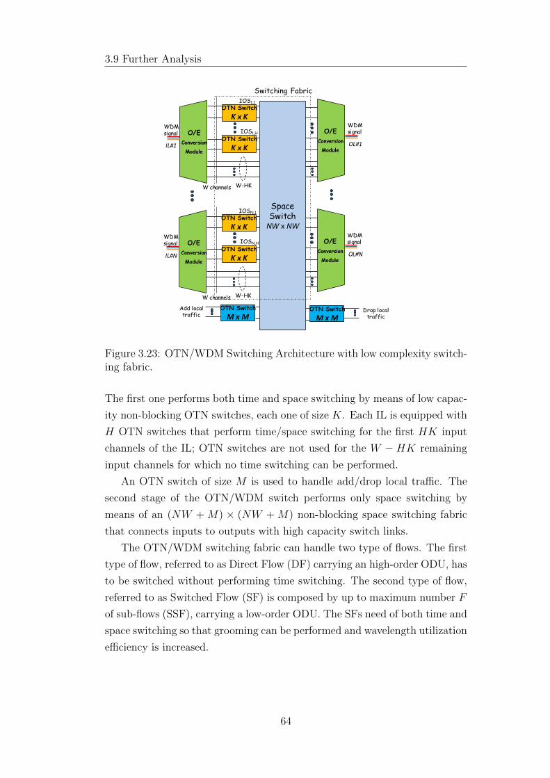
3.9 Further Analysis
Drop local traffic
OTN Switch
M x M OTN Switch
M x M Add local traffic
Space Switch
NW x NW
IOS1,1
W channels
OTN Switch
K x K
OTN Switch
K x K
IOS1,H
IL#1
WDM signal
OL#1
WDM signal
W-HK
IOSN,1
W channels
OTN Switch
K x K
OTN Switch
K x K
IOSN,H
IL#N
O/E
Conversion
Module
WDM signal
OL#N
WDM signal
W-HK
O/E
Conversion
Module
O/E
Conversion
Module
O/E
Conversion
Module
Switching Fabric
Figure 3.23: OTN/WDM Switching Architecture with low complexity switch-ing fabric.
The first one performs both time and space switching by means of low capac-
ity non-blocking OTN switches, each one of size K. Each IL is equipped with
H OTN switches that perform time/space switching for the first HK input
channels of the IL; OTN switches are not used for the W − HK remaining
input channels for which no time switching can be performed.
An OTN switch of size M is used to handle add/drop local traffic. The
second stage of the OTN/WDM switch performs only space switching by
means of an (NW + M) × (NW + M) non-blocking space switching fabric
that connects inputs to outputs with high capacity switch links.
The OTN/WDM switching fabric can handle two type of flows. The first
type of flow, referred to as Direct Flow (DF) carrying an high-order ODU, has
to be switched without performing time switching. The second type of flow,
referred to as Switched Flow (SF) is composed by up to maximum number F
of sub-flows (SSF), carrying a low-order ODU. The SFs need of both time and
space switching so that grooming can be performed and wavelength utilization
efficiency is increased.
64

3.9 Further Analysis
3.9.1 Numerical Results
The blocking performance of the 12-nodes RING and 13-nodes DENSE
metropolitan networks, illustrated in Figs 3.24.a and 3.24.b respectively and
assuming each wavelength channel carries ODU-2 at 10 Gbps, have been
evaluated by simulation.
(a) (b)
Figure 3.24: RING network (a) and DENSE network (b).
In these analysis, the networks are equipped with the integrated OT-
N/WDM switching nodes proposed in Section 3.9. To evaluate the perfor-
mance degradation that the blocking switching fabric of the proposed solution
introduces, the results are compared to the ones obtained when non blocking
switching fabric are taken into account. Two typologies of flows are offered
to the network nodes: flows carrying ODU-2 (10 Gbps) and subflows carrying
ODU-0 (1.25 Gbps).
According to the OTN standard, up to F=8 ODU-0 can be carried on an
ODU-2. In this case, the traffic is assumed to be uniformly distributed among
all node pairs; both the request inter-arrival time and the connection duration
are exponentially distributed. Let α the average bandwidth percentage of
ODU-0 offered. The average offered bandwidth traffic intensity normalized
to the network capacity is given by
A0 =Λ
FWL
∑sd
hsd
, where L is the number of bidirectional fiber links, W is the number of
wavelength channels, Λ is the offered bandwidth traffic between two any nodes
and hsd is the hop count of the shortest path between the nodes s,d.
In this analysis, the important assumption is that the routing of any con-
nection carrying ODU-0 (ODU-2) between the nodes s and d is performed
according to the following steps:
65

3.9 Further Analysis
Figure 3.25: Network blocking probability versus the average bandwidthpercentage of ODU-0 offered in the case of RING network, in the case ofnodes equipped with Non Blocking Switching Fabric (NBSF) and the Block-ing Switching Fabric (BSF) of Fig. 3.23 and H varying from 1 to 4.
Figure 3.26: Network blocking probability versus the average bandwidth per-centage of ODU-0 offered in the case of DENSE network, in the case ofnodes equipped with Non Blocking Switching Fabric (NBSF) and the Block-ing Switching Fabric (BSF) of Fig. 3.23 and H varying from 1 to 4.
66
3.9 Further Analysis
i) the shortest path between the nodes s and d is chosen;
ii) an auxiliary graph is built having nodes representing OTN switches
and fictitious nodes representing the wavelength bundle in which OTN
switches are absent;
iii) two any graph nodes are connected if free resources (high capacity switch
link and wavelengths) are available to carry ODU-0 (ODU-2) between the
OTN switches/wavelength bundles representing the nodes;
iv) weights are assigned to the graph edge so that the routing of ODU-2 is
performed by using preferably wavelengths in which OTN switches are
absent and the routing of ODU-0 is performed by using preferably high
capacity switch links and wavelengths already carrying other ODU-0’s;
v) a new shortest path is evaluated in the auxiliary graph between the nodes
representing the add and drop OTN switches of the nodes s and d re-
spectively; if any shortest path exists, the connection is routed choosing
at random free resources (wavelength and ODU container) through the
OTN switches and the wavelength bundles corresponding to the nodes
of the evaluated path, otherwise the connection request is rejected.
Figs 3.25 and 3.26 plot the network blocking probability as a function of α
in the case of the RING and DENSE metropolitan networks having a number
L of unidirectional fiber links equal to 24 and 40 respectively. Each link
carries W=48 wavelengths and A0 is equal to 0.60 and 0.25 for the RING and
DENSE networks. In these figure, the blocking probability in the case of an
integrated OTN/WDM optical switch with Blocking Switching Fabric (BSF)
characterized by the use of available market OTN switches of size K=12 are
reported. The number H of OTN switches is varied from 1 to 4 where H=4
corresponds to the case in which all of the wavelengths are equipped with
OTN switches. It is also plotted the blocking probability obtained in the case
in which Non Blocking Switching Fabrics (NBSF) are used. From Figs 3.25
and 3.26 we can observe that in the case H=4 the degradation in blocking
probability due to the use of blocking switching fabrics is higher in the case of
DENSE networks. This is due to its higher average network degree that leads
to a lower average available number of high capacity switch links ongoing an
OTN switch per Output Line [14] and consequently a higher blocking. We
can notice from figs 3.25 and 3.26 that a correct dimensioning procedure can
67
3.10 CONCLUSIONS
lead to a reduction of OTN switches. As a matter of example we can use in
the case of DENSE network only half (H=2) of the OTN switches per node
when the average bandwidth percentage α of ODU-0 offered is smaller than
or equal to 50%.
3.10 CONCLUSIONS
In Section 3.1. an integrated OTN/WDM switching architecture provided
with spatial speedup has been studied and its complexity has been evaluated
in terms of number of OTN switches and space switching modules used. The
ILP formulation of the Switch Resource Assignment and Routing Problem al-
lowed us to verify the effectiveness of an heuristic, referred to as Maximizing
Shortest Path Traffic that it is used to evaluate the network blocking perfor-
mance of large networks in static traffic scenario when ODU-2 and ODU-0
traffic is considered. The obtained results have shown that in these traffic
conditions the use of spatial speedup is not needed because the basic switch
without speedup allows for the same network blocking performance obtained
with Strict Sense Non Blocking switches.
A simulation analysis has been carried out to evaluate the blocking prob-
ability of different metropolitan networks in dynamic traffic condition. In
this case a remarkable performance degradation can occur. For example, in
a network with 13 nodes and 40 fibers, equipped with W=48 wavelengths,
and the normalized offered bandwidth traffic intensity is 0.091 the network
blocking probability is equal to 1.80 · 10−4 and 1.44 · 10−6 in the case of basic
and NBSS switches respectively. The results reported in Section 3.4 show that
this performance degradation due to the switch internal blocking however can
be overcome with the use of spatial speedup equal to 1.5 that consequently
increases the hardware complexity of the proposed switch, but allowing for
a high complexity reduction with respect to the case of Strict Sense Non
Blocking switch.
Furthermore, Section 3.5 deals with an integrated OTN/WDM switching
architecture with a reduced number of OTN switches. Then an heuristic, re-
ferred to as Minimizing OTN Switch Resource (MOSR), has been introduced
to evaluate the network blocking performance in static traffic scenario. The
results obtained in a 34-nodes metropolitan network show that when the L-
ODU fraction of offered traffic bandwidth demand is equal to 0.4, it is possible
to save the 50% and 15% of OTN switches and 144 × 144 crosspoints with
68

3.10 CONCLUSIONS
respect to the case in which all of the OTN switches are used.
69

Chapter 4
Xhaul Architecture in C-RAN
Environment
4.1 Introduction
Cloud Radio Access Network (C-RAN) or Centralized RAN could be con-
sidered one of the most promising solutions for its efficiency and flexibility
[4, 5]. Based on the idea to physically separate the traditional base sta-
tion in the two different entities Base Band Unit (BBU) and Remote Radio
Unit (RRU), C-RAN leads to important advantages, as energy saving, To-
tal Cost of Ownership (TCO) saving, improving security and deployment of
infrastructure ready to support advanced features, like Coordinated Multi-
Point (CoMP), enhanced inter-cell interference coordination (eICIC), carrier
aggregation and more complex and dynamic multiple-input multiple-output
(MIMO) schemes [6, 7].
The access network is represented by the “fronthaul” that connects the
BBUs with the RRUs. The most used standard to encapsulate radio samples
is the Common Public Radio Interface (CPRI), that needs much bandwidth
to carry the CPRI flows that have a bit rate up to ten times higher than
the total capacity of a traditional base station. It is clear that the network
architecture, both access and transport, and its control need to be rethought.
An emerging network paradigm, labeled as “Xhaul” [13], wraps fronthaul
and backhaul in a common connectivity segment providing a joint optimiza-
tion opportunity, especially in sharing transport resources for different pur-
poses and protocols. Xhaul unifies and enhances the traditional backhaul
and fronthaul areas by enabling a flexible deployment and reconfiguration of
71
4.1 Introduction
network elements and networking functions. The role of the Xhaul transport
network is to convey Ethernet traffic and CPRI traffic on the same network
infrastructure.
In this chapter, a network solution in which the radio component is com-
posed by RRU and traditional Radio Base Station (RBS) has been analyzed.
The conducted study shows that the solution in which only RRUs are used
are not cost effectiveness because the low power consumption achieved with
the switching off of the centralized components does not compensate the high
bandwidth consumption. Conversely the use of only RBSs would lead to
bandwidth efficient solutions but very poor in terms of power consumption.
In the next sections, the main contributions of the analysis [15] are ex-
plained and, in particular, they could be summarized in the following way:
i) the definition of analytical models, validated by simulation, for the re-
source dimensioning of the Xhaul network;
ii) the evaluation of power/bandwidth trade-off solutions based on the op-
timal determination of the percentage of RRUs to be used in order to
minimize the sum of the bandwidth and power costs.
Furthermore, several traffic models characterizing the statistical of the
peak traffic values [3] are introduced. According to these traffic models, a
dimensioning procedure is illustrated allowing significantly lower number of
CPRI circuits as well as the number of BBUs needed, with respect to the case
in which that number is statically fixed to the number of installed RRUs. This
study aims at quantifying the potential advantages in terms of bandwidth and
energy saving obtainable via:
i) an activation/deactivation policy of BBUs associated to the sub-areas;
ii) a full sharing of transport capacity in the Xhaul network.
The reference scenario considered in the reported analysis is reported in
Section 4.2.
In the rest of chapter, two different solutions are considered and analyzed.
The first reported solution is based on the use of a reconfigurable fronthaul
network (only CPRI solution) that owing to statistical multiplexing advan-
tages allows for bandwidth savings in order to balance the advantages in power
saving and the remarkable bandwidth consumption. The proposed solution
has been investigated with the introduction of an analytical model allowing
72

4.2 Proposed Xhaul Architecture
for the dimensioning of the needed CPRI flows and consequently the evalu-
ation of the bandwidth and power consumptions. Then the main results for
forecast 5G network areas are illustrated in Section 4.5.2.
To the other hand, a solution for a reconfigurable Xhaul network is also
proposed and investigated. The cost evaluation model is reported in Section
4.3 and the dimensioning analytical models are reported in Section 4.4. In
particular, the description of the traffic modeling, the network dimensioning
procedure and the resource modeling are reported in Sections 4.4.1 and 4.4.2
for the CPRI and GEth flows respectively. The main results for 4G and
forecast 5G network areas are illustrated in Section 4.5.
Finally conclusions and future research items are illustrated in Section 4.6.
4.2 Proposed Xhaul Architecture
Figure 4.1: Xhaul Network Architecture
This section deals with the Xhaul architecture [15] reported in Fig. 4.1.
As said in the introduction, the Xhaul architecture unifies the traditional
backhaul and fronthaul areas by enabling a flexible deployment and recon-
73

4.2 Proposed Xhaul Architecture
Parameter Description
BCPRI bandwidth required by one CPRI flow
KBBU maximum number of BBU instances supported inany BBU server
CRRU capacity of an RRU
CRBS capacity of a micro RBS
nRRU number of RRUs installed in a sub-area
nRBS number of micro RBSs installed in a sub-area
T number of sub-areas handled by an AS
nASRRU =TnRRU
number of RRUs installed in the region handled bythe AS
nASRBS =TnRBS
number of micro RBSs installed in the regionhandled by the AS
Table 4.1: Network parameters in Xhaul reference architecture
figuration of networks elements and networking functions, providing a joint
optimization opportunity, especially between transport resources and energy
consumption. It handles a reference area divided in macro areas, each one
covered by macro base station (macro BS). Each macro area is divided into
sub-areas, each one covered by a certain number of RRUs and traditional
micro base stations (micro RBSs). A reference area is handled by a Central
Office (CO) that contains a certain number of BBU servers managed by a
Control and Management (“C&M”) module. The “C&M” has the role of ac-
tivating/deactivating/migrating BBU instances in the BBU servers with each
BBU instance related to an active RRU, and moreover of implementing algo-
rithms for the consolidation of BBU instances that lead to save energy. In the
CO, Ethernet switch is also located to handle the Ethernet traffic generated
by the micro RBSs.
Central office and radio stations (RRU and micro RBS) are connected to
the BBUs by a reconfigurable transport network though some Access Switch
(AS) and one HUB switch a shown in Fig. 4.1. Thus the Xhaul network has
two levels:
• the first one, defined as “access network”, connects the several RRUs
and micro RBSs with the closest element of aggregation, referred to as
Access Switch (AS);
74

4.2 Proposed Xhaul Architecture
Figure 4.2: Access Switch Architecture
• the second one, defined as “reconfigurable network”, connects the Access
Nodes with the HUB switch placed in the Central Office.
The network reconfiguration allows for a bandwidth saving and this may
occur on a hourly basis according to the traffic variations. The reconfigu-
ration capability of ASs and the HUB switch provides a flexible allocation
of the bandwidth and server resources to the RRUs and micro RBSs. Effi-
cient implementations of reconfigurable networks consider solutions that com-
bines DWDM and OTN, whose benefits are largely studied in several works
[54, 56, 57, 58, 59, 71, 86, 87, 79], enabling hybrid transport of CPRI and
Ethernet flows.
Example of AS and HUB switch architectures are reported in Figs 4.2
and 4.3 respectively. The AS is composed by a Reconfigurable Optical Add
Drop Multiplexer (ROADM), an agnostic cross connect switch, the CPRI
and Ethernet Switches. In particular the agnostic cross connect is inserted
for scalability reasons and only allows for the spatial switching of CPRI and
Ethernet aggregated flows. The flows generated by the RRU (micro RBS) are
handled by the CPRI (Ethernet) switch, and forwarded towards the CO by
appropriately configuring the agnostic cross connect switch and the ROADM.
The HUB switch, as described in Fig. 4.3, is composed by an agnostic cross
connect switch and by CPRI and Ethernet switches. Each input/output
WDM interface of the agnostic cross connect switch is connected to a ROADM
ring. The CPRI switch is connected to the BBU server pools.
An integrated OTN/WDM architecture could be used to implement the
agnostic cross connect switches presented in the previous solutions, in order
to manage the different kind of traffic in a large flexible way, guaranteeing
the same performances as ROADM. [14, 80, 81, 82, 85, 83, 88].
75
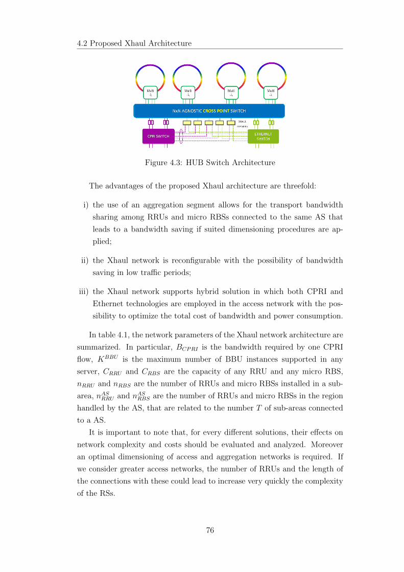
4.2 Proposed Xhaul Architecture
Figure 4.3: HUB Switch Architecture
The advantages of the proposed Xhaul architecture are threefold:
i) the use of an aggregation segment allows for the transport bandwidth
sharing among RRUs and micro RBSs connected to the same AS that
leads to a bandwidth saving if suited dimensioning procedures are ap-
plied;
ii) the Xhaul network is reconfigurable with the possibility of bandwidth
saving in low traffic periods;
iii) the Xhaul network supports hybrid solution in which both CPRI and
Ethernet technologies are employed in the access network with the pos-
sibility to optimize the total cost of bandwidth and power consumption.
In table 4.1, the network parameters of the Xhaul network architecture are
summarized. In particular, BCPRI is the bandwidth required by one CPRI
flow, KBBU is the maximum number of BBU instances supported in any
server, CRRU and CRBS are the capacity of any RRU and any micro RBS,
nRRU and nRBS are the number of RRUs and micro RBSs installed in a sub-
area, nASRRU and nASRBS are the number of RRUs and micro RBSs in the region
handled by the AS, that are related to the number T of sub-areas connected
to a AS.
It is important to note that, for every different solutions, their effects on
network complexity and costs should be evaluated and analyzed. Moreover
an optimal dimensioning of access and aggregation networks is required. If
we consider greater access networks, the number of RRUs and the length of
the connections with these could lead to increase very quickly the complexity
of the RSs.
76
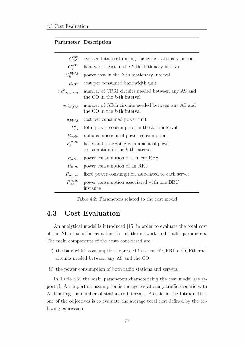
4.3 Cost Evaluation
Parameter Description
Cavgtot average total cost during the cycle-stationary period
CBWk bandwidth cost in the k-th stationary interval
CPWRk power cost in the k-th stationary interval
µBW cost per consumed bandwidth unit
nckAS,CPRI number of CPRI circuits needed between any AS andthe CO in the k-th interval
nckAS,GE number of GEth circuits needed between any AS andthe CO in the k-th interval
µPWR cost per consumed power unit
P ktot total power consumption in the k-th interval
Pradio radio component of power consumption
PBBUk baseband processing component of power
consumption in the k-th interval
PRBS power consumption of a micro RBS
PRRU power consumption of an RRU
Pserver fixed power consumption associated to each server
PBBUins power consumption associated with one BBU
instance
Table 4.2: Parameters related to the cost model
4.3 Cost Evaluation
An analytical model is introduced [15] in order to evaluate the total cost
of the Xhaul solution as a function of the network and traffic parameters.
The main components of the costs considered are:
i) the bandwidth consumption expressed in terms of CPRI and GEthernet
circuits needed between any AS and the CO;
ii) the power consumption of both radio stations and servers.
In Table 4.2, the main parameters characterizing the cost model are re-
ported. An important assumption is the cycle-stationary traffic scenario with
N denoting the number of stationary intervals. As said in the Introduction,
one of the objectives is to evaluate the average total cost defined by the fol-
lowing expression:
77
4.3 Cost Evaluation
Cavgtot =
1
TN
N−1∑k=0
(CBWk + CPWR
k ) (4.1)
where CBWk and CPWR
k denote the bandwidth and power consumption cost
in the k − th (k = 0, · · · , N − 1) stationary interval. As you can notice from
(4.1), the cost contribution due to MBS is not taken into account. This is
due to the fact that this contribution has no significance impact on the cost
optimization procedure that is carried out later.
For the contribution CBWk we can simply write:
CBWk = µBW (nckAS,GE + nckAS,CPRI ·BCPRI) (4.2)
wherein µBW is the cost per consumed bandwidth unit, nckAS,GE and
nckAS,CPRI are the number of GEth flows (that hold 1 Gbps traffic) and CPRI
flows between any AS and the CO needed in the k-th interval respectively,
BCPRI is the bandwidth required (in Gbps) by one CPRI flow.
The second contribution CPWRk can be simply expressed as follows:
CPWRk = µPWRP
totk (4.3)
wherein µPWR is the cost per consumed power unit and P totk is the total
power consumption in the k-th stationary interval.
The total power consumption is evaluated considering the sum of several
contributions, related to the radio and baseband processing components Pradio
and PBBUk respectively. We can write:
P totk = Pradio + PBBU
k (4.4)
For the radio component Pradio, the power consumption is assumed to be
independent of the handled traffic according to the today’s technology. Let
us denote with PRBS and PRRU the power consumption of micro RBS and
RRUs respectively. Thus we can simply write:
Pradio = PRBS · nASRBS + PRRU · nASRRU (4.5)
wherein nASRBS and nASRRU are the parameters introduced in Section 4.2 and
denoting the number of micro RBSs and RRUs handled by any AS respec-
tively.
78
4.4 Analytical Models for Resource Dimensioning in Xhaul Architecture
The second contribution PBBUk can be defined as the sum of a fixed contri-
bution for the server rack (power supply, conditioned air, etc.) and a variable
contribution related to the BBU instance processing. The fixed contribution
is related to both the used number of servers and the fixed power consumption
associated to each server (Pserver), whereas the variable one is related to the
number of BBU instances (equal to the number of needed CPRI flows) and
the power consumption associated with one BBU instance (PBBUins ). In this
analysis, the variable component of the power consumption is assumed to be
a linear function of the processing capacity. Hence, the power consumption
PBBUk related to the baseband processing can be expressed as follows:
PBBUk = Pserver ·
⌈nckAS,CPRIKBBU
⌉+ PBBU
ins · nckAS,CPRI (4.6)
wherein KBBU is the maximum number of BBU instances supported in
any server.
Finally by inserting (4.5) and (4.6) in (4.4), (4.4) in (4.3), (4.2) and (4.3)
in (4.1) we can achieve the average total cost Cavgtot .
You can notice how the knowledge of nckAS,GE and nckAS,CPRI is needed
for the evaluation of Cavgtot . These parameters characterize the number of
GEthernet and CPRI circuits needed between any AS and the CO and are
determined according to a dimensioning procedure illustrated in the next
Section 4.4.
4.4 Analytical Models for Resource Dimen-
sioning in Xhaul Architecture
This section introduces the resource dimensioning models for the case in
which the operation mode of the Xhaul architecture is the following:
• the installed micro RBSs are always turned on and provide a basic
capacity for the coverage of the sub-area;
• the installed RRUs are always turned on and provides additional capac-
ity needed in the intervals in which the traffic increases; the RRUs are
only used when the basic capacity provides by the micro RBSs is not
sufficient to support the user traffic; for this reason BBU instances are
only instanced for the corresponding RRUs used; a server consolidation
79
4.4 Analytical Models for Resource Dimensioning in Xhaul Architecture
algorithm is applied in order to minimize, in each stationary interval,
the number of switched on servers.
The introduced analytical models allow us to evaluate the number nckAS,GEand nckAS,CPRI of GEthernet and CPRI circuits respectively needed between
any AS and the CO. The number nckAS,GE and nckAS,CPRI are important to
make the network planning of the access network in each hour interval that
gives informations for dimensioning the transport network. The evaluation of
the number of needed circuits is based on the following traffic assumptions:
• the traffic is cycle-stationary with N stationary periods; for instance N
equals 24 when the classical daily traffic variation has to be reproduced;
• the user peak traffic generated in the sub-areas, expressed in Gbps, are
independent and identically distributed (i.i.d.) variables; therefore the
user peak traffic generated in any sub-area in the k-th stationary interval
is characterized by a variable Ak that according to [89] we assume log-
normal distributed of parameters (µk, σk);
Next the number nckAS,GE and nckAS,CPRI of GEthernet and CPRI circuits
are evaluated in Subsections 4.4.1 and 4.4.2 respectively.
4.4.1 Evaluation of the number nckAS,CPRI of CPRI cir-
cuits
The decrease in offered traffic and the application of the switching off
technique of BBU instances leads to the need of carrying a number of CPRI
flows lower the number of installed RRUs.
To evaluate the values nckAS,CPRI (k = 0, 1, ..., N − 1), we could start by
the knowledge of the statistical on the number NkAS (k = 0, 1, ..., N − 1),
denoting the sum of used RRUs in the region handled by the AS in the k-
th interval. In Appendix A.3.1, it is shown how it is possible to evaluate
the probabilities pNkAS
(j) (j = 0, 1, ..., T · nRRU) of the random variable NkAS.
Hence the dimensioning of the number nckAS,CPRI of CPRI circuits between
the AS and and CO in the k-th interval is performed by guaranteeing high
the probability of the event that a number of used RRUs is lower than or
equal to nckAS,CPRI . In other words, nckAS,CPRI has been chosen as the α-th
percentile of NkAS (k = 0, 1, ..., N − 1) that is the smallest value for which the
following expression holds:
80

4.5 Numerical Results
Pr(NkAS ≤ nckAS,CPRI) ≥ 0.01 · α (k = 0, 1, ..., N − 1) (4.7)
We can equivalently write (4.7) in terms of survivor function of NkAS as
follows:
Pr(NkAS > nckAS,CPRI) < 1− 0.01 · α (k = 0, 1, ..., N − 1) (4.8)
4.4.2 Evaluation of the number nckAS,GE of GEthernet
circuits
In Appendix A.3.2, it is shown how it is possible to evaluate the statistical
of the number NkAS,E (k = 0, 1, ..., N − 1) of GEthernet flows to be carried
between the AS and and CO. In particular we are able to evaluate the prob-
abilities of NkAS,E denoted as pNk
AS,E(j) (j = 0, 1, · · · , dT · nRBS · CRBSe). As
in the case of dimensioning of CPRI circuits, nckAS,GE has been chosen as the
α-th of NkAS,E (k = 0, 1, ..., N − 1) that is the smallest value for which the
following expression holds:
Pr(NkAS,E > nckAS,GE) < 1− 0.01 · α (k = 0, 1, ...N − 1) (4.9)
4.5 Numerical Results
The objective of this study is not only to evaluate the advantages in terms
of CPRI flow bandwidth consumption saving that a reconfigurable optical
network allows us to achieve when strategies for the BBU instance switching
off are applied, but also to evaluate a trade-off between employment of RRUs
and micro RBSs with regard to the energy and bandwidth consumption.
As depicted in Fig. 4.4, the reference scenario is an area of 1 km2 handled
by a central office that contains a certain number of BBU servers. We assume
that the area is divided into squared sub-areas, where in each of them there is
a building surrounded by streets and squares. Each sub-area is covered with a
given number of RRUs and micro RBSs, that generate CPRI and GEthernet
flows respectively.
This scenario assumption is suited to model a broadband access in dense
urban areas [3]. In fact, the proposed study considers a dense outdoor area
(streets, square) and an indoor ultra-high broadband access area, related to a
81
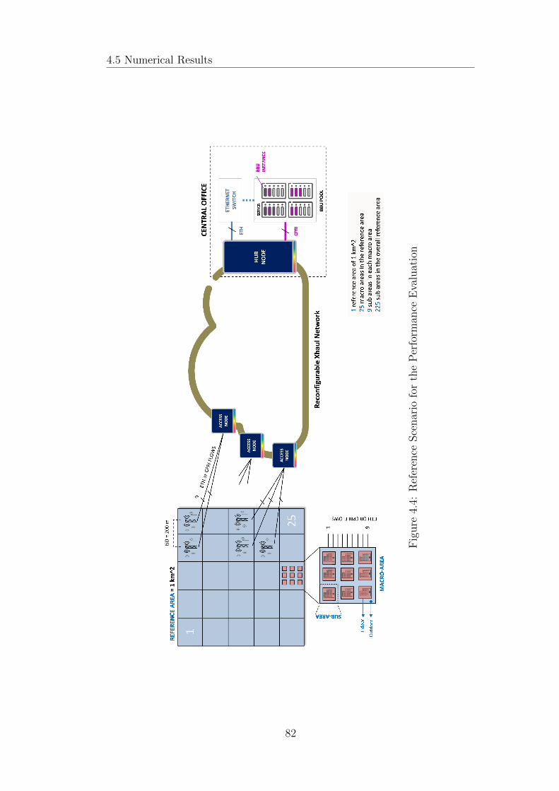
4.5 Numerical Results
Fig
ure
4.4:
Ref
eren
ceSce
nar
iofo
rth
eP
erfo
rman
ceE
valu
atio
n
82
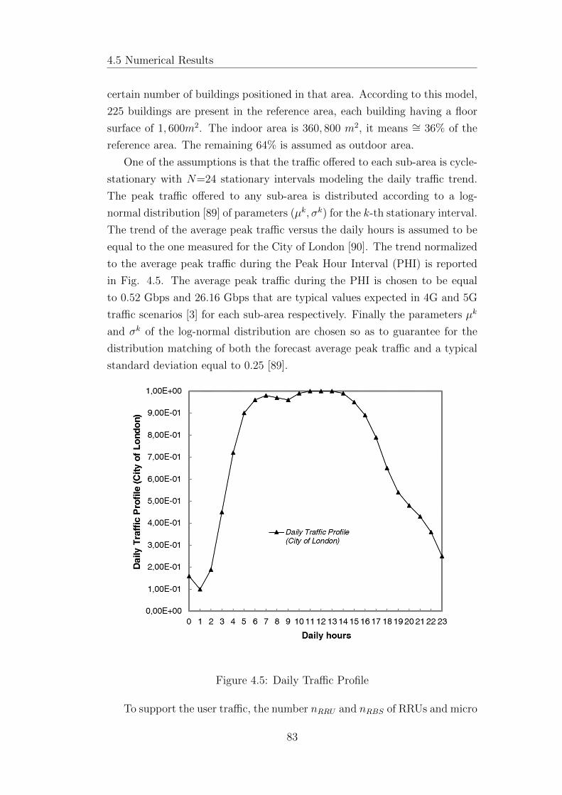
4.5 Numerical Results
certain number of buildings positioned in that area. According to this model,
225 buildings are present in the reference area, each building having a floor
surface of 1, 600m2. The indoor area is 360, 800 m2, it means ∼= 36% of the
reference area. The remaining 64% is assumed as outdoor area.
One of the assumptions is that the traffic offered to each sub-area is cycle-
stationary with N=24 stationary intervals modeling the daily traffic trend.
The peak traffic offered to any sub-area is distributed according to a log-
normal distribution [89] of parameters (µk, σk) for the k-th stationary interval.
The trend of the average peak traffic versus the daily hours is assumed to be
equal to the one measured for the City of London [90]. The trend normalized
to the average peak traffic during the Peak Hour Interval (PHI) is reported
in Fig. 4.5. The average peak traffic during the PHI is chosen to be equal
to 0.52 Gbps and 26.16 Gbps that are typical values expected in 4G and 5G
traffic scenarios [3] for each sub-area respectively. Finally the parameters µk
and σk of the log-normal distribution are chosen so as to guarantee for the
distribution matching of both the forecast average peak traffic and a typical
standard deviation equal to 0.25 [89].
Figure 4.5: Daily Traffic Profile
To support the user traffic, the number nRRU and nRBS of RRUs and micro
83

4.5 Numerical Results
RBSs installed in each sub-area are dimensioned according to the procedure
illustrated in Appendix A.3.3. It is denoted with γ the ratio of the number
nRRU of RRUs to the total number nRRU + nRBS of radio stations, that is:
γ =nRRU
nRBS + nRRU(4.10)
Next Sections 4.5.1 and 4.5.2 deal with the network resource dimension-
ing and bandwidth/power costs in the case of the reconfigurable fronthaul
architecture in 5G scenario, in which only CPRI flows are carried. For the
Xhaul architecture, some network resource dimensioning results are in Sec-
tion 4.5.3 while bandwidth/power trade-off solutions will be investigated in
Section 4.5.4.
4.5.1 Network Dimensioning in Fronthaul Architecture
In a fronthaul architecture, a traditional C-RAN solution is implemented,
thus only RRUs are installed in the sub-areas. In this case, we can consider
the same analytical models presented in the previous sections and a value of
γ equal to 0.
For a 5G scenario, it is assumed that an LTE bandwidth equal to 20
MHz and MIMO 8x8 are assigned to each station. RRUs are characterized
by a capacity of CRRU=600 Mbps. Each RRU generates one CPRI flow
@10Gbps [11]. If the dimensioning of RRUs is performed so as to guarantee
the α=99.99th percentile of the user peak traffic offered to the sub-area, we
achieve the values nRRU = 107.
If RRU switching off strategies were not applied, it would be needed to
guarantee a number of CPRI circuits equal to the number nCPRIAS of hardware
elements generating CPRI traffic and tied to the AS. The values of nCPRIAS
is equal to nASRRU that is given by T times the value of nRRU . In this case
we achieve a value of 3375 for nCPRIAS . Conversely a remarkable reduction in
CPRI circuits is possible to achieve if switching off algorithms are adopted.
In Appendix-A.3.1 the survivor function of the variable NkAS has been eval-
uated for each stationary interval and by applying the procedure mentioned in
Section 4.3, the number of CPRI circuits to be supported between the Access
Switch and the CO. It has verified that the application of the dimensioning
procedure allows for a remarkable saving with respect to the case in which
the dimensioning is performed on the number RRUs installed. For instance
the percentage advantage in terms of CPRI circuits in the Peak Hour Interval
84
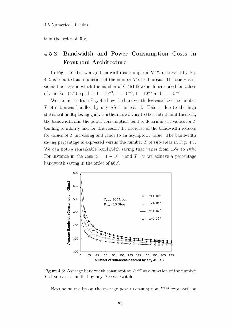
4.5 Numerical Results
is in the order of 30%.
4.5.2 Bandwidth and Power Consumption Costs in
Fronthaul Architecture
In Fig. 4.6 the average bandwidth consumption Bavg, expressed by Eq.
4.2, is reported as a function of the number T of sub-areas. The study con-
siders the cases in which the number of CPRI flows is dimensioned for values
of α in Eq. (4.7) equal to 1− 10−3, 1− 10−5, 1− 10−7 and 1− 10−9.
We can notice from Fig. 4.6 how the bandwidth decrease how the number
T of sub-areas handled by any AS is increased. This is due to the high
statistical multiplexing gain. Furthermore owing to the central limit theorem,
the bandwidth and the power consumption tend to deterministic values for T
tending to infinity and for this reason the decrease of the bandwidth reduces
for values of T increasing and tends to an asymptotic value. The bandwidth
saving percentage is expressed versus the number T of sub-areas in Fig. 4.7.
We can notice remarkable bandwidth saving that varies from 45% to 70%.
For instance in the case α = 1 − 10−5 and T=75 we achieve a percentage
bandwidth saving in the order of 66%.
300
350
400
450
500
550
600
5 25 45 65 85 105 125 145 165 185 205 225
Ave
rag
e B
an
dw
idth
Co
ns
um
pti
on
(G
bp
s)
Number of sub-areas handled by any AS (T )
CRRU=600 Mbps
BCPRI=10 Gbps
=1-10-3
=1-10-5
=1-10-7
=1-10-9
Figure 4.6: Average bandwidth consumption Bavg as a function of the numberT of sub-area handled by any Access Switch.
Next some results on the average power consumption P avg expressed by
85

4.5 Numerical Results
40
45
50
55
60
65
70
5 25 45 65 85 105 125 145 165 185 205 225
Ba
nd
wid
th S
avin
g P
erc
en
tag
e (
%)
Number of sub-areas handled by any AS (T )
=1-10-3
=1-10-5
=1-10-7
=1-10-9
CRRU=600 Mbps
BCPRI=10 Gbps
Figure 4.7: Bandwidth saving percentage as a function of the number T ofsub-area handled by any Access Switch.
Eq. (4.3) are reported. The results are evaluated by considering the model
reported in Section 4.3 and a total power consumption PRRU,BBU of a CPRI
network element equal to the constant value 300 Watt. PRRU,BBU is expressed
by:
PRRU,BBU = PRRU + Pserver/KBBU + PBBUins (4.11)
The value of KBBU is chosen equal to 4 while the constant server power
Pserver is fixed equal to 30% of the maximum server power. Furthermore
it is denoted with δ the ratio of the radio power consumption PRRU to the
total power consumption PRRU,BBU . It is important to note that the RRU
is always on, thus only the baseband processing component gives a variable
contribution to the total power consumption.
The average power consumption P avg, expressed by Eq. (4.3) is reported
in Fig. 4.8 as a function of the number T of sub-area and varying the ratio
δ of constant radio power consumption from 0.2 to 0.8. Even in this case we
can notice how the statistical multiplexing effect, due to processing resource
sharing of the BBU instances, leads to a decrease in power consumption for
T increasing. Furthermore we notice how the power consumption is as much
higher as the value of the radio power consumption PRRU . As a matter of
example, for T=45 we achieve values of P avg equal to 154W and 279W for
86

4.5 Numerical Results
δ = 0.2 and δ = 0.8 respectively. The reason of this effect is due to lower
advantage in statistical multiplexing due to the increase in power consumption
of the radio resources that are not shared.
Figure 4.8: Average power consumption P avg as a function of the number Tof sub-area handled by any Access Switch. The ratio δ of the radio powerconsumption PRRU to the total power consumption PRRU,BBU of an RRU ischosen equal to 0.2, 0.4, 0.6 and 0.8.
4.5.3 Network Dimensioning in Xhaul Architecture
Next some dimensioning results for the Xhaul architecture are reported
in the case of a AS handling the traffic of T=45 sub-areas. Both 4G and 5G
traffic scenario will be considered in order to show the very high differences
between these two scenarios and the goodness of our approach in both of
them.
In the 4G scenario case, the considered assumption is that an LTE band-
width equal to 20 MHz and MIMO 2x2 are assigned to each station. RRUs
are characterized by a capacity of CRRU=150 Mbps. Each RRU generates one
CPRI flow @2.5Gbps [11]. Micro RBSs are also employed with capacity of
CRBS = 150 Mbps. The ratio γ of the number of RRUs to the total number
of radio stations is chosen equal to 0.7. If the dimensioning of RRUs and
micro RBSs is performed so as to guarantee the α=99.99th percentile of the
87
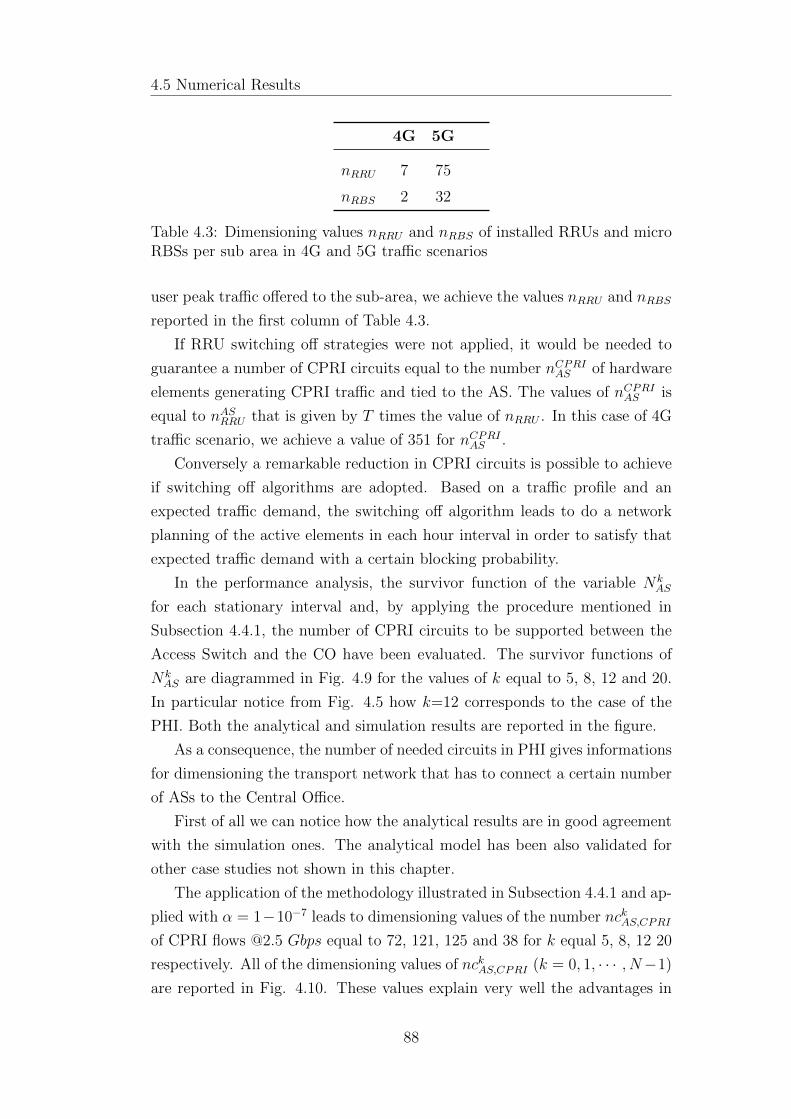
4.5 Numerical Results
4G 5G
nRRU 7 75
nRBS 2 32
Table 4.3: Dimensioning values nRRU and nRBS of installed RRUs and microRBSs per sub area in 4G and 5G traffic scenarios
user peak traffic offered to the sub-area, we achieve the values nRRU and nRBS
reported in the first column of Table 4.3.
If RRU switching off strategies were not applied, it would be needed to
guarantee a number of CPRI circuits equal to the number nCPRIAS of hardware
elements generating CPRI traffic and tied to the AS. The values of nCPRIAS is
equal to nASRRU that is given by T times the value of nRRU . In this case of 4G
traffic scenario, we achieve a value of 351 for nCPRIAS .
Conversely a remarkable reduction in CPRI circuits is possible to achieve
if switching off algorithms are adopted. Based on a traffic profile and an
expected traffic demand, the switching off algorithm leads to do a network
planning of the active elements in each hour interval in order to satisfy that
expected traffic demand with a certain blocking probability.
In the performance analysis, the survivor function of the variable NkAS
for each stationary interval and, by applying the procedure mentioned in
Subsection 4.4.1, the number of CPRI circuits to be supported between the
Access Switch and the CO have been evaluated. The survivor functions of
NkAS are diagrammed in Fig. 4.9 for the values of k equal to 5, 8, 12 and 20.
In particular notice from Fig. 4.5 how k=12 corresponds to the case of the
PHI. Both the analytical and simulation results are reported in the figure.
As a consequence, the number of needed circuits in PHI gives informations
for dimensioning the transport network that has to connect a certain number
of ASs to the Central Office.
First of all we can notice how the analytical results are in good agreement
with the simulation ones. The analytical model has been also validated for
other case studies not shown in this chapter.
The application of the methodology illustrated in Subsection 4.4.1 and ap-
plied with α = 1−10−7 leads to dimensioning values of the number nckAS,CPRIof CPRI flows @2.5 Gbps equal to 72, 121, 125 and 38 for k equal 5, 8, 12 20
respectively. All of the dimensioning values of nckAS,CPRI (k = 0, 1, · · · , N−1)
are reported in Fig. 4.10. These values explain very well the advantages in
88
4.5 Numerical Results
the application of a switching off technique with respect to the case in which
the dimensioning is performed on the number RRUs installed. For instance
when k=12, that is in the PHI, the percentage advantage in terms of CPRI
circuits is in the order of 64%.
Furthermore, in the Fig 4.10, it is reported the validation of the analytic
results obtained through a simulation campaign.
Figure 4.9: Survivor Function of the random variables NkAS for k equal to 5,
8, 12 and 20 in a 4G traffic scenario. Both analytical and simulation resultsare reported.
The results for the dimensioning of the number nckAS,GE of GEthernet
circuits are also reported in Fig 4.11. In this figure, it is shown the num-
ber of GEthernet circuits needed between the AS and the CO in each daily
time interval. We can see a remarkable reduction in number of GEthernet
circuits in the daily intervals when the traffic is very low. For instance in
the time interval k = 2 only 3 GEthernet circuits are needed instead of 14 if
the dimensioning were dimensioned according to the capacity of micro RBSs
installed.
Next some results for a 5G traffic scenario are presented. In this case the
traffic density is much higher. To handle this remarkable traffic amount, the
89
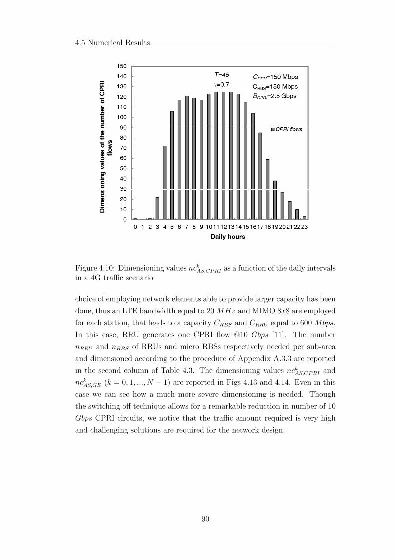
4.5 Numerical Results
Figure 4.10: Dimensioning values nckAS,CPRI as a function of the daily intervalsin a 4G traffic scenario
choice of employing network elements able to provide larger capacity has been
done, thus an LTE bandwidth equal to 20 MHz and MIMO 8x8 are employed
for each station, that leads to a capacity CRBS and CRRU equal to 600 Mbps.
In this case, RRU generates one CPRI flow @10 Gbps [11]. The number
nRRU and nRBS of RRUs and micro RBSs respectively needed per sub-area
and dimensioned according to the procedure of Appendix A.3.3 are reported
in the second column of Table 4.3. The dimensioning values nckAS,CPRI and
nckAS,GE (k = 0, 1, ..., N − 1) are reported in Figs 4.13 and 4.14. Even in this
case we can see how a much more severe dimensioning is needed. Though
the switching off technique allows for a remarkable reduction in number of 10
Gbps CPRI circuits, we notice that the traffic amount required is very high
and challenging solutions are required for the network design.
90

4.5 Numerical Results
Figure 4.11: Dimensioning values nckAS,GE as a function of the daily intervalsin a 4G traffic scenario
4.5.4 Optimal Bandwidth/Power Consumption Trade-
Off
Next some results evaluated by the model reported in Section 4.3 are re-
ported. In the Xhaul solution analysis as in the case of the fronthaul solution,
the RBS power consumption PRBS is considered equal to 300 Watt ([91, 92])
and the same value for the total power consumption PRRU,BBU of a CPRI
network element is assumed. In the same way, PRRU,BBU is expressed by:
PRRU,BBU = PRRU + Pserver/KBBU + PBBUins
The value of KBBU is chosen equal to 4 while the constant server power
Pserver is fixed equal to 30% of the maximum server power. Furthermore, also
in this case, it is denoted with δ the ratio of the radio power consumption
PRRU to the total power consumption P totRRU,BBU . It is important to note that
the RRU is always on, thus only the baseband processing component gives
a variable contribution to the total power consumption. Here the objective
is to evaluate the optimum value of γ allowing for a right trade-off between
91

4.5 Numerical Results
Figure 4.12: Survivor Function of the random variables NkRS for k equal to 5,
8, 12 and 20 in a 5G traffic scenario
bandwidth and power consumption. Obviously the study depends on the
values of the parameters µBW and µPWR introduced in Section 4.3 and char-
acterizing the costs per bandwidth unit (1 Gbps) and per power unit (1 W)
respectively. In particular we have noticed that when µBW=1, the region in
which the trade-off exists is when µPWR ranges from 0.001 to 0.86. In fact
when µPWR is smaller (larger) than 0.001 (0.86), the bandwidth cost (power
cost) is dominant and we have the trivial solution γ=0 (γ=1), in which only
micro RBSs (RRUs) are used.
In Fig. 4.15 the bandwidth and power consumption costs are reported and
evaluated given by the two contributions of the second hand of expression (4.2)
for µBW=1, µPWR=0.01, δ=0.5 and when T=45 sub-areas are handled by an
AS. In Fig. 4.15 it is also presented the total cost expressed by (4.2). As it
is possible to note, the power consumption decreases when the γ ratio of the
number nRRU of RRUs to the total number of radio stations increases. In fact
when this increase occurs a larger number of RRUs is used in place of RBSs
and it is possible to save the energy consumption related to the deactivation of
BBU instances that are not used when the traffic is low. At the same time we
notice that the increase of γ leads to bandwidth cost increases very quickly due
to the high bandwidth required by the CPRI flows. As reported in Fig. 4.15,
92
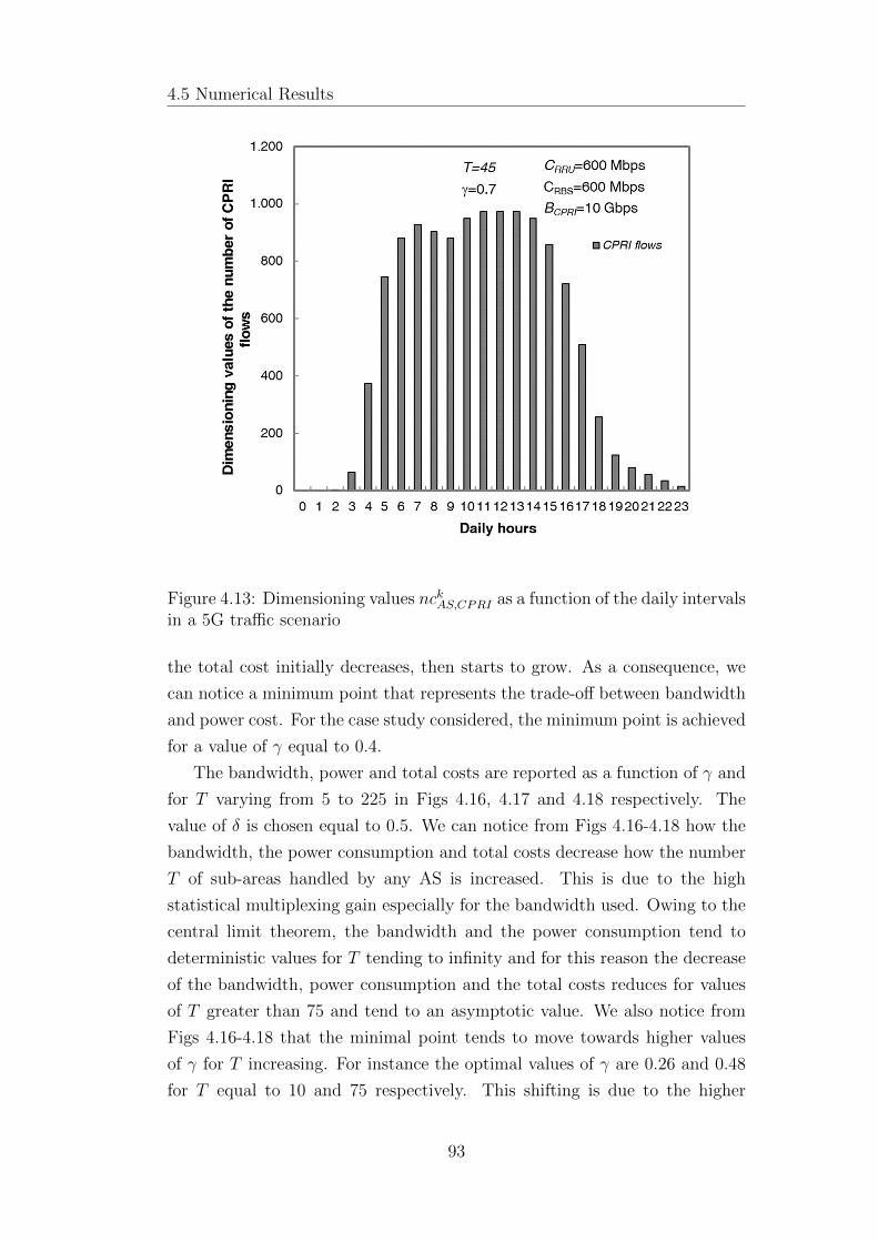
4.5 Numerical Results
Figure 4.13: Dimensioning values nckAS,CPRI as a function of the daily intervalsin a 5G traffic scenario
the total cost initially decreases, then starts to grow. As a consequence, we
can notice a minimum point that represents the trade-off between bandwidth
and power cost. For the case study considered, the minimum point is achieved
for a value of γ equal to 0.4.
The bandwidth, power and total costs are reported as a function of γ and
for T varying from 5 to 225 in Figs 4.16, 4.17 and 4.18 respectively. The
value of δ is chosen equal to 0.5. We can notice from Figs 4.16-4.18 how the
bandwidth, the power consumption and total costs decrease how the number
T of sub-areas handled by any AS is increased. This is due to the high
statistical multiplexing gain especially for the bandwidth used. Owing to the
central limit theorem, the bandwidth and the power consumption tend to
deterministic values for T tending to infinity and for this reason the decrease
of the bandwidth, power consumption and the total costs reduces for values
of T greater than 75 and tend to an asymptotic value. We also notice from
Figs 4.16-4.18 that the minimal point tends to move towards higher values
of γ for T increasing. For instance the optimal values of γ are 0.26 and 0.48
for T equal to 10 and 75 respectively. This shifting is due to the higher
93

4.5 Numerical Results
Figure 4.14: Dimensioning values nckAS,GE as a function of the daily intervalsin a 5G traffic scenario
decrease in bandwidth with respect to power consumption when the number
T of sub-areas handled by an AS is increased.
As further contribution to the investigation done in this work, in Fig. 4.19
the total cost is reported as a function of γ when T=45 and for values of δ
equal to 0.20, 0.40, 0.60 and 0.80. We can notice from Fig. 4.19 how the
minimal points moves towards lower values of γ for δ increasing. As a matter
of example, the minimum values of γ equal 0.55 and 0.42 for T equal to 0.20
and 0.80 respectively. The reason is due to higher radio power consumption
PRRU of an RRU that makes less power efficient the use of RRUs.
Finally, the conducted analysis considers the impact on the cost of a spa-
tial correlation of the traffic distribution. In particular, the case in which the
spatial correlation coefficient has a negative exponential trend [93] as a func-
tion of the distance between sub-areas has been studied. Next it is denoted
with ρ the correlation coefficient of the traffic of two adjacent sub-areas. Fig.
4.20 shows the survivor function of the number of needed CPRI flows when
an AS handles T=45 sub-areas and for values of ρ varying from 0 to 0.6. The
5G traffic scenario is considered and the values of k equal to 12 and 20 are
94
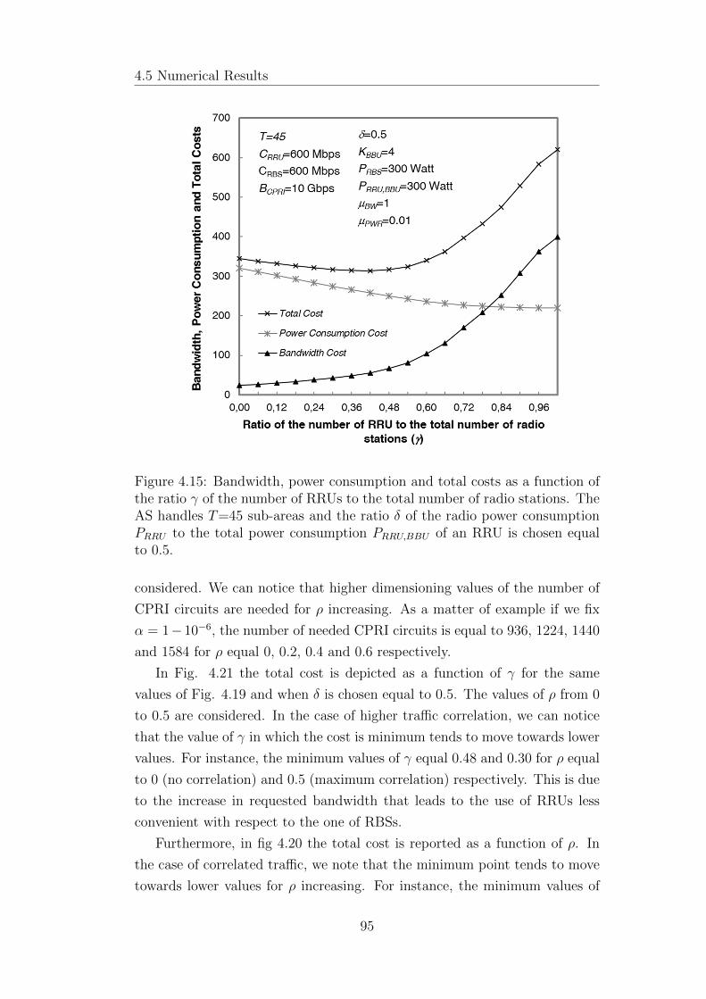
4.5 Numerical Results
Figure 4.15: Bandwidth, power consumption and total costs as a function ofthe ratio γ of the number of RRUs to the total number of radio stations. TheAS handles T=45 sub-areas and the ratio δ of the radio power consumptionPRRU to the total power consumption PRRU,BBU of an RRU is chosen equalto 0.5.
considered. We can notice that higher dimensioning values of the number of
CPRI circuits are needed for ρ increasing. As a matter of example if we fix
α = 1−10−6, the number of needed CPRI circuits is equal to 936, 1224, 1440
and 1584 for ρ equal 0, 0.2, 0.4 and 0.6 respectively.
In Fig. 4.21 the total cost is depicted as a function of γ for the same
values of Fig. 4.19 and when δ is chosen equal to 0.5. The values of ρ from 0
to 0.5 are considered. In the case of higher traffic correlation, we can notice
that the value of γ in which the cost is minimum tends to move towards lower
values. For instance, the minimum values of γ equal 0.48 and 0.30 for ρ equal
to 0 (no correlation) and 0.5 (maximum correlation) respectively. This is due
to the increase in requested bandwidth that leads to the use of RRUs less
convenient with respect to the one of RBSs.
Furthermore, in fig 4.20 the total cost is reported as a function of ρ. In
the case of correlated traffic, we note that the minimum point tends to move
towards lower values for ρ increasing. For instance, the minimum values of
95

4.6 Conclusions
Figure 4.16: Bandwidth cost as a function of the ratio γ of the number ofRRUs to the total number of radio stations. The ratio δ of the radio powerconsumption PRRU to the total power consumption PRRU,BBU of an RRU ischosen equal to 0.5 and the AS handles a number T of sub-areas varying from5 to 225.
γ equal 0.48 and 0.30 for ρ equal to 0 (no correlation) and 0.5 (maximum
correlation) respectively. This is due to the assumptions that the RBSs are
always active and give a basic capacity thus, if their number is higher, the
access network capacity could be enough to menage more traffic in case of
correlated event.
4.6 Conclusions
In this chapter, a dimensioning procedure has been proposed to evaluate
the number of CPRI and GEthernet circuits that a network has to guarantee
between an Access Switch and the CO. The AS handles the traffic generated
by a set of sub-areas. The user traffic is managed by both micro RBSs and
RRUs that generate GEthernet and CPRI flows respectively. The dimension-
ing procedure allows for a saving of needed CPRI circuits with respect to the
case in which the number of CPRI circuits is statically fixed to the number
96
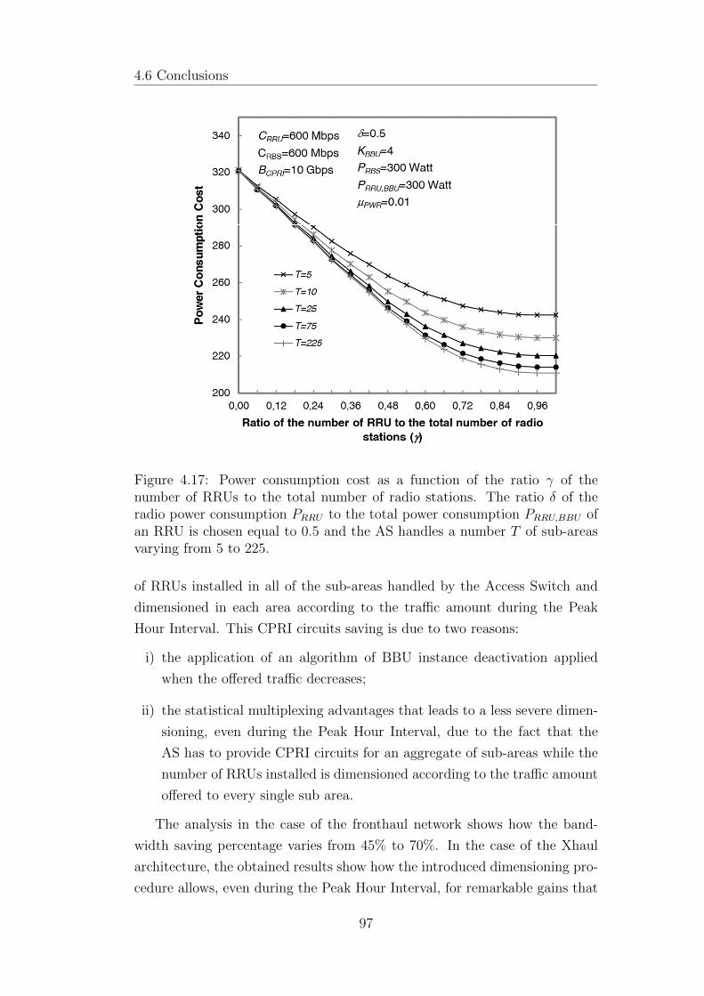
4.6 Conclusions
Figure 4.17: Power consumption cost as a function of the ratio γ of thenumber of RRUs to the total number of radio stations. The ratio δ of theradio power consumption PRRU to the total power consumption PRRU,BBU ofan RRU is chosen equal to 0.5 and the AS handles a number T of sub-areasvarying from 5 to 225.
of RRUs installed in all of the sub-areas handled by the Access Switch and
dimensioned in each area according to the traffic amount during the Peak
Hour Interval. This CPRI circuits saving is due to two reasons:
i) the application of an algorithm of BBU instance deactivation applied
when the offered traffic decreases;
ii) the statistical multiplexing advantages that leads to a less severe dimen-
sioning, even during the Peak Hour Interval, due to the fact that the
AS has to provide CPRI circuits for an aggregate of sub-areas while the
number of RRUs installed is dimensioned according to the traffic amount
offered to every single sub area.
The analysis in the case of the fronthaul network shows how the band-
width saving percentage varies from 45% to 70%. In the case of the Xhaul
architecture, the obtained results show how the introduced dimensioning pro-
cedure allows, even during the Peak Hour Interval, for remarkable gains that
97
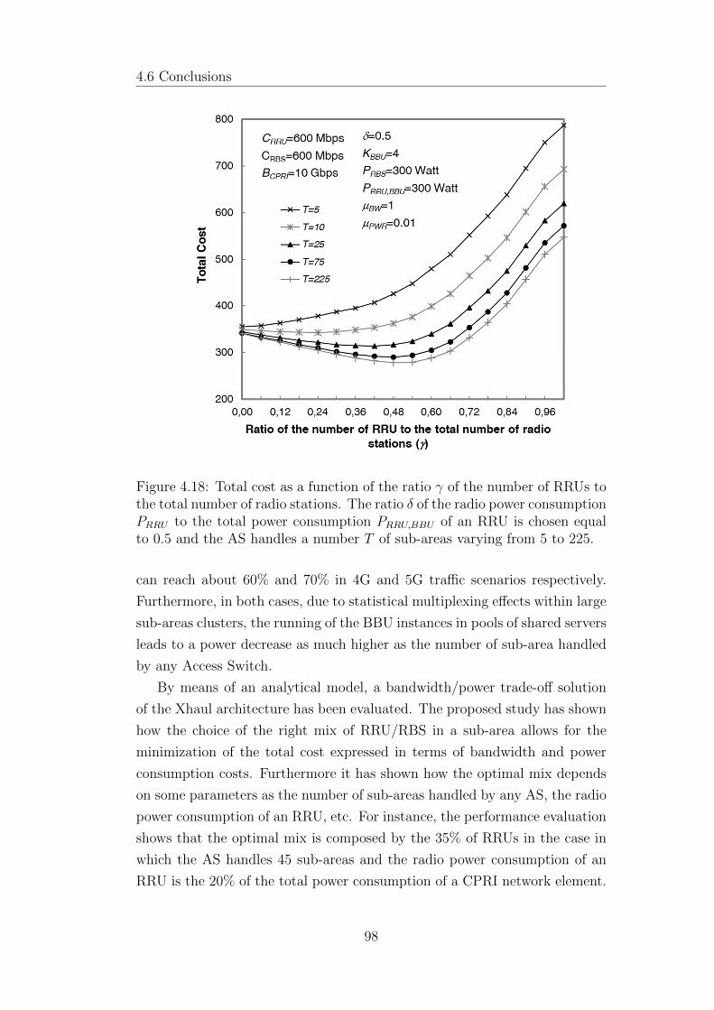
4.6 Conclusions
Figure 4.18: Total cost as a function of the ratio γ of the number of RRUs tothe total number of radio stations. The ratio δ of the radio power consumptionPRRU to the total power consumption PRRU,BBU of an RRU is chosen equalto 0.5 and the AS handles a number T of sub-areas varying from 5 to 225.
can reach about 60% and 70% in 4G and 5G traffic scenarios respectively.
Furthermore, in both cases, due to statistical multiplexing effects within large
sub-areas clusters, the running of the BBU instances in pools of shared servers
leads to a power decrease as much higher as the number of sub-area handled
by any Access Switch.
By means of an analytical model, a bandwidth/power trade-off solution
of the Xhaul architecture has been evaluated. The proposed study has shown
how the choice of the right mix of RRU/RBS in a sub-area allows for the
minimization of the total cost expressed in terms of bandwidth and power
consumption costs. Furthermore it has shown how the optimal mix depends
on some parameters as the number of sub-areas handled by any AS, the radio
power consumption of an RRU, etc. For instance, the performance evaluation
shows that the optimal mix is composed by the 35% of RRUs in the case in
which the AS handles 45 sub-areas and the radio power consumption of an
RRU is the 20% of the total power consumption of a CPRI network element.
98
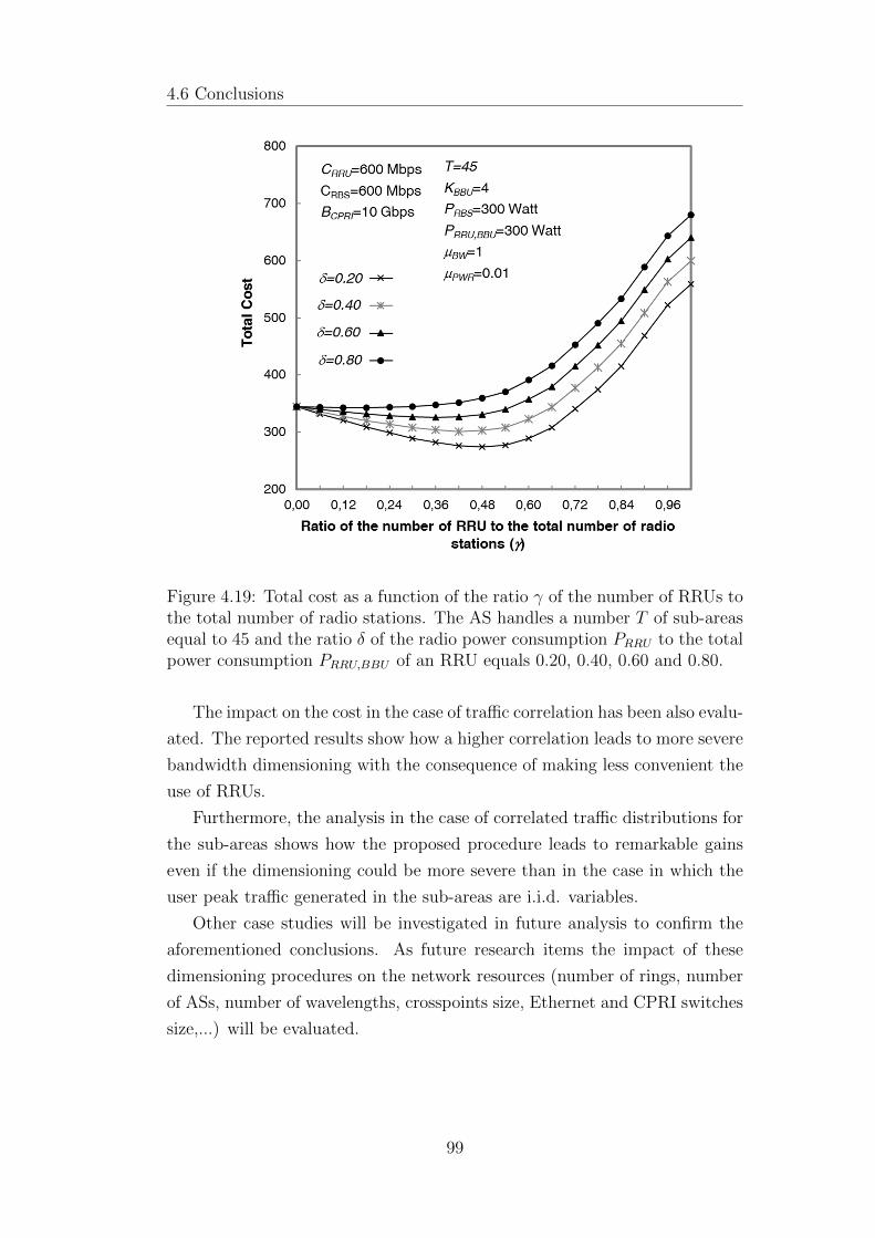
4.6 Conclusions
Figure 4.19: Total cost as a function of the ratio γ of the number of RRUs tothe total number of radio stations. The AS handles a number T of sub-areasequal to 45 and the ratio δ of the radio power consumption PRRU to the totalpower consumption PRRU,BBU of an RRU equals 0.20, 0.40, 0.60 and 0.80.
The impact on the cost in the case of traffic correlation has been also evalu-
ated. The reported results show how a higher correlation leads to more severe
bandwidth dimensioning with the consequence of making less convenient the
use of RRUs.
Furthermore, the analysis in the case of correlated traffic distributions for
the sub-areas shows how the proposed procedure leads to remarkable gains
even if the dimensioning could be more severe than in the case in which the
user peak traffic generated in the sub-areas are i.i.d. variables.
Other case studies will be investigated in future analysis to confirm the
aforementioned conclusions. As future research items the impact of these
dimensioning procedures on the network resources (number of rings, number
of ASs, number of wavelengths, crosspoints size, Ethernet and CPRI switches
size,...) will be evaluated.
99

4.6 Conclusions
Figure 4.20: Survivor Function of the random variables NkAS for k equal to
12 and 20 in a 5G traffic scenario where the spatial correlation parameter ρvaries from 0 to 0.6
100

4.6 Conclusions
Figure 4.21: Total cost as a function of the ratio γ of the number of RRUsto the total number of radio stations. The AS handles a number T of sub-areas equal to 45, the ratio δ of the radio power consumption PRRU to thetotal power consumption PRRU,BBU of an RRU equals to 0.50 and the spatialcorrelation parameter ρ varies from 0 to 0.5
101

Chapter 5
Conclusions and Outlooks
In this thesis, the trend evolution and the road toward the 5G networks
have been explored. It has been analyzed the transition from the vision of
a transparent all-optical network to a more versatile and pragmatic idea of
network that can handle efficiently different radio access technologies, whose
the next generation network will be the best expression.
Some of the key drivers of this evolution are the increase of the mobile
networks capacity, the data rates and the number of devices simultaneously
connected, and the requirements for extremely low latency to provide for a
better user experience, energy efficiency, or the centralization of control in
order to accommodate more complex network planning and optimization and
to simplify the hardware enabling the virtualization of the network functions.
In adding to these ones, we could consider the capacity of the future network
to reconfigure itself in order to achieve some of the goals listed above. It
is clear to understand that the network needs to be as flexible as possible to
manage in the same architecture the several types of radio access technologies.
Flexibility is, in facts, one of the key points of this research. The joint
use of OTN/WDM switching is one of the available solutions to manage the
very heterogeneous technologies of the next generation access network. The
advantages introduced by the OTN/WDM integrated switching are related to
the finer granularity of this technology compared to the all-optical switches.
This benefits could be exploit to obtain high level of efficiency and, of course,
flexibility.
For these reasons, a low complex integrated OTN/WDM switch node has
been studied and evaluated. In this analysis, some architectures are consid-
ered and the savings in terms of number of components has been evaluated
through the formulations of routing and assignment problems and the in-
103

troduction of heuristics for simulations. Network blocking performance have
been evaluated for different metropolitan networks and in static and dynamic
scenarios. It has also been estimated the right spatial speedup that the archi-
tecture needs in order to compensate the performance degradation due the
switch internal blocking and save components, thus allowing for hardware
complexity reduction, with respect to the case of Strict Sense Non Blocking
switch.
The second part of the thesis deals with the investigation of a network
architecture, called “Xhaul”, that unifies fronthaul and backhaul networks in
a common connectivity segment. A dimensioning procedure has been pro-
posed to evaluate the number of CPRI (fronthaul) and GEthernet (backhaul)
circuits that a network has to guarantee between an Access Switch and the
Central Office. In particular, this procedure allows for a saving of needed
CPRI circuits with respect to the case in which the number of CPRI circuits
is statically fixed. The achievement of this bandwidth efficiency is due to
two important reasons: the application of BBU instance deactivation policies
when the offered traffic decreases, and the statistical multiplexing advantages
that leads to a less severe dimensioning, even during the Peak Hour Interval.
The analysis shows how the introduced procedure allows for remarkable gains
that can reach about 60% and 70% in 4G and 5G traffic scenarios respectively.
By means of an analytical model, a bandwidth/power trade-off solution
of the Xhaul architecture has been evaluated. The proposed study has shown
how the choice of the right mix of RRU/RBS in a sub-area allows for the
minimization of the total cost expressed in terms of bandwidth and power
consumption costs. Furthermore it has shown how the optimal mix depends
on some parameters as the number of sub-areas handled by any AS, the radio
power consumption of an RRU, etc. For instance, the performance evaluation
shows that the optimal mix is composed by the 35% of RRUs in the case in
which the AS handles 45 sub-areas and the radio power consumption of an
RRU is the 20% of the total power consumption of a CPRI network element.
The impact on the cost in the case of traffic correlation has been also evalu-
ated. The reported results show how a higher correlation leads to more severe
bandwidth dimensioning with the consequence of making less convenient the
use of RRUs.
Furthermore, the analysis in the case of correlated traffic distributions for
the sub-areas shows how the proposed procedure leads to remarkable gains,
even if the dimensioning could be more severe than in the case in which the
104

user peak traffic generated in the sub-areas are i.i.d. variables.
Other case studies will be investigated in future analysis to confirm the
aforementioned conclusions. As future research items, it will be evaluated the
impact of these dimensioning procedures on the network resources (number
of rings, number of ASs, number of wavelengths, crosspoints size, Ethernet
and CPRI switches size,etc.).
105

Appendix A
Appendices
A.1 Proof of the lemma 1 on the SSNB con-
dition of the switch core
Lemma 1: Under the constraint of W multiple of H, the proposed switch
core architecture is SSNB if the speedup S is greater than or equal to
SSSNB = d KbKFce
Proof. The assumption is that at a given instant the worst traffic conditions
according to which:
i) only SH-ODU traffic is offered to the switch;
ii) the maximum number NWF − 1 of L-ODUs is already handled by the
switch and hence there is one only input wavelength and one only output
wavelength that can carry one L-ODU.
These wavelengths are referred to as λfi and λfo respectively. We have to
determine the minimum value SSSNB of the spatial speedup so that there are
sufficient switch resources to carry the L-ODU from λfi to λfo .
Let us suppose that λfi to λfo are an input and an output of the OTN
switches denoted as IOSx,y and OSSz,t respectively. The minimum value
SSSNB is obtained when the following two conditions occur:
1. the NWF −1 L-ODUs already handled by the switch, engage the max-
imum number NIOSx,y
OM and NOOSz,t
IM of outputs and inputs of IOSx,y and
OOSz,t respectively;
1

A.1 Proof of the lemma 1 on the SSNB condition of the switch core
2. one input and one output of IOSx,y and OOSz,t respectively are still
available.
The OTN switching modules IOSx,y and OOSz,t handle WH
input and
output wavelengths channels respectively and WHF − 1 L-ODUs. In the worst
case these L-ODUs are carried on different interstage links and hence need
the engagement of NIOSx,y
OM =NOOSz,t
IM =WHF − 1 outputs and inputs of IOSx,y
(OOSz,t) respectively.
The evaluation of NIOSx,y
OM and NOOSz,t
IM and the conditions 1) and 2) lead
to the condition K=WHF and that is to the following condition for SSSNB:
SSSNB =
⌈K⌊KF
⌋⌉ (A.1)
2

A.2 Proof of the lemma 2 on the SSNB condition of the space switchingmodule
A.2 Proof of the lemma 2 on the SSNB con-
dition of the space switching module
Lemma 2: A U × U switching module with a three stages NBSS Clos
network structure can be realized with the least number NQ×Q of Q × Q
(U > Q) switching modules given by:
NQ×Q = minn∈Θ
2
⌈ ⌈Un
⌉⌊Q
2n−1
⌋⌉+
2n− 1⌊
Q
dUn e
⌋ (A.2)
where Θ is a set of positive integer numbers given by:
Θ = i ∈ Z+ / Q ≥ max(2i− 1,
⌈U
i
⌉) (A.3)
Proof. To prove expression (A.2), in Fig. A.1 it is reported a three stages
SSNB Clos network with dUne n× (2n− 1) switching elements in the first and
third stage and (2n− 1) dUne × dU
ne switching elements in the second stage.
While the parameter U is given, we can optimize the choice of the pa-
rameter n. The Clos network is realized with the available Q × Q switching
modules by aggregating switching elements of the Clos network as indicated
in Fig. A.1. Thus the number NQ×Q(n) of Q × Q switching modules for a
given n could be expressed as:
NQ×Q(n) = N1stQ×Q(n) +N2nd
Q×Q(n) +N3rdQ×Q(n) (A.4)
where N1stQ×Q(n), N2nd
Q×Q(n) and N3rdQ×Q(n) are the number of Q×Q switching
modules needed for the first, second and third stage of the Clos Network for a
given n. N1stQ×Q(n) and N3rd
Q×Q(n) can be expressed according to the following
remarks:
i) each Q×Q switching module can implement up to d Q2n−1e n× (2n− 1)
switching elements of the first and third stage;
ii) these stages contain each one a number dUne of switching elements.
Hence we can write:
N1stQ×Q(n) = N3rd
Q×Q(n) =
⌈ ⌈Un
⌉⌊Q
2n−1
⌋⌉ (A.5)
3
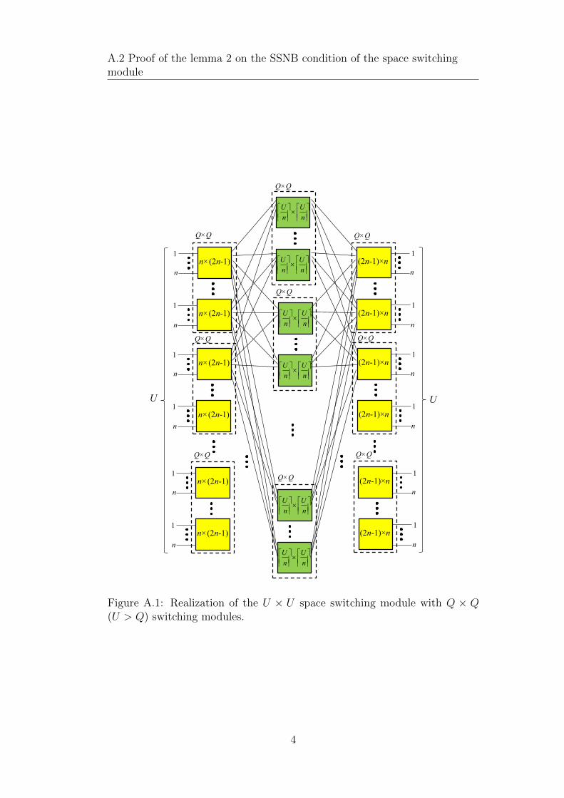
A.2 Proof of the lemma 2 on the SSNB condition of the space switchingmodule
1
n
n×(2n-1)
1n×(2n-1)
n
Q×Q
1
n
n×(2n-1)
1n×(2n-1)
n
1
n
n×(2n-1)
1n×(2n-1)
n
1
n
(2n-1)×n
1(2n-1)×n
n
1
n
(2n-1)×n
1(2n-1)×n
n
1
n
(2n-1)×n
1(2n-1)×n
n
×
n
U
n
U
×
n
U
n
U
×
n
U
n
U
×
n
U
n
U
×
n
U
n
U
×
n
U
n
U
Q×Q
Q×Q
Q×Q
Q×Q
Q×Q
Q×Q
Q×Q
Q×Q
U U
Figure A.1: Realization of the U × U space switching module with Q × Q(U > Q) switching modules.
4

A.2 Proof of the lemma 2 on the SSNB condition of the space switchingmodule
To guarantee that the introduction of the Q×Q switching modules does
not introduce any blocking, we have to impose that the Q × Q switching
module allow for the aggregation of at least one n×(2n−1) switching element.
That leads to the following condition:
Q ≥ 2n− 1 (A.6)
By analogy to expressions (A.5) and (A.6), we can write for the second
stage:
N2ndQ×Q(n) =
2n− 1⌊
Q
dUn e
⌋ (A.7)
Q ≥⌈U
n
⌉(A.8)
Finally by inserting (A.5) and (A.7) in (A.4) and minimizing with respect
to the parameter n we obtain (A.2). By taking into account (A.6) and (A.8),
it follows that the optimization of n has to be searched in the set given by
(A.3).
5
A.3 Xhaul Evaluation Analysis
A.3 Xhaul Evaluation Analysis
A.3.1 Evaluation of the probabilities pNkAS
(j) of the ran-
dom variable NkAS
If as reference we consider an Access Switch that handles the traffic of T
sub-areas, and we denote with Nkt the number of CPRI circuits needed for the
sub-area SAt (t = 1, ..., T ), the following expression for NkAS can be written:
NkAS =
T∑t=1
Nkt (k = 0, 1, ...N − 1) (A.9)
The lack of traffic correlation assumed, leads to i.i.d random variables
Nkt (t = 1, ..., T ). Then we can write the following expression (A.10) for the
probabilities Nkt :
pNkAS
(j) = ⊗TpNkSA
(j) j = 1, ..., TnRRU k = 0, 1, ...N − 1 (A.10)
wherein pNkSA
(h) denotes the probabilities of Nkt and the symbol ⊗T de-
notes the convolution operator applied T times.
For the evaluation of the probability pNkSA
(h) (h = 0, 1, ..., nRRU), that is
the probability that h RRUs are used in the target sub-area, we remember
our assumption of minimizing the number of CPRI circuits that leads to
employing as much as possible the capacity of micro RBSs and only when
this capacity is occupied, RRU capacity is used.
Next we consider three cases:
i) h = 0;
ii) 1 ≤ h ≤ nRRU − 1;
iii) h = nRRU .
In the case h = 0, we can observe that NkSA is equal to 0 up to when the
traffic Ak offered to the sub-area is smaller than or equal to nRBS CRBS that
is the total sum of the capacities of the nRBS micro RBSs assigned to the
target sub-area.
In the case 1 ≤ h ≤ nRRU − 1, we can observe that NkSA is equal to h
when the traffic Ak offered to the sub area is in the interval [nRBSCRBS +
(h− 1)CRRU , nRBS CRBS + h CRRU ].
6
A.3 Xhaul Evaluation Analysis
In the case h = nRRU , we can observe that NkSA is equal to nRRU when
the offered traffic is higher than or equal to nRBSCRBS + nRRUCRRU .
According to the observations above, the expression A.11 could be ob-
tained for the probabilities pNkSA
(h) (h = 0, 1, ..., nRRU). Finally by in-
serting (A.11) in (A.10), we can evaluate the probabilities pNkAS
(j) (j =
0, 1, ..., TnRRU) of the random variable NkAS.
A.3.2 Evaluation of the probabilities pNkAS,E
(j) of the
random variable NkAS,E
If as reference we consider an Access Switch that handles the traffic of T
sub-areas, NkAS,E denotes the number of GEthernet flows that depends on the
traffic generated by the micro RBSs located in the sub-areas. To evaluate the
probabilities pNkAS,E
(j) we need to knowledge the total traffic amount (Gbps)
AkAS,E expressed in Gbps and emitted by the micro RBSs handled by the
AS. If we denote with AkSAtthe traffic amount generated by the micro RBSs
located in the sub area SAt (t = 1, ..., T ), the following expression holds:
AkAS,E =T∑t=1
AkSAt(k = 0, 1, ..., N − 1) (A.13)
It is assumed that the random variables AkSAt(t = 1, ..., T ) independent
and identically distributed (i.i.d.) with log-normal distributions of parameters
(µk, σk). In this case it has been proved that the probability density pAkAS,E
(x)
of AkAS,E can be approximated as log-normal probability density of parameters
(µkAS, σkAS) given by the following expressions [94]:
σkAS =
√loge(
1
T(e(σk)2 − 1) + 1) (A.14)
µkAS = loge(Teµk) + 0.5((σk)2 − (σkAS)2) (A.15)
At this point we can evaluate the probabilities pNkAS,E
(j) (j =
1, ..., dTnRBSCRBSe) from the probability densities pAkAS,E
(x) of the random
variable AkAS,E. We can follow the same approach applied in Appendix-A.3.1
and obtain the expression (A.12).
7
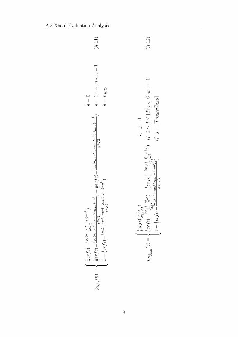
A.3 Xhaul Evaluation Analysis
p Nk SA
(h)
=
1 2erfc(−
loge(n
RBSC
RBS
)−µk
σk√
2)
h=
0
1 2erfc(−
loge(n
RBSC
RBS
+hC
RRU
)−µk
σk√
2)−
1 2erfc(−
loge(n
RBSC
RBS
+(h−
1)C
RRU
)−µk
σk√
2)
h=
1,···,nRRU−
1
1−
1 2erfc(−
loge(n
RBSC
RBS
+nRRUC
RRU
)−µk
σk√
2)
h=nRRU
(A.1
1)
p Nk AS,E
(j)
=
1 2erfc(
µk AS
σk AS
√2)
ifj
=1
1 2erfc(−
logej−µk AS
σk AS
√2
)−
1 2erfc(−
loge(j−
1)−µk AS
σk AS
√2
)if
2≤j≤dTnRBSCRBSe−
1
1−
1 2erfc(−
loge(dTnRBSC
RBSe−
1)−µk AS
σk AS
√2
)if
j=dTnRBSCRBSe
(A.1
2)
8
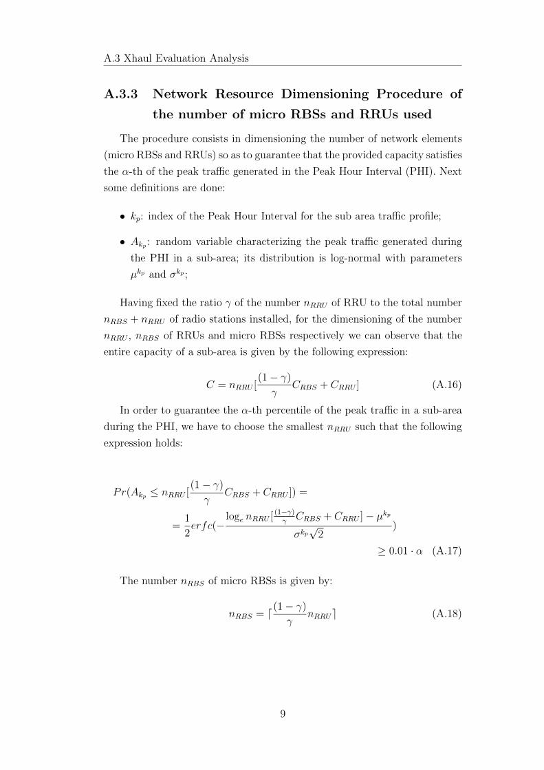
A.3 Xhaul Evaluation Analysis
A.3.3 Network Resource Dimensioning Procedure of
the number of micro RBSs and RRUs used
The procedure consists in dimensioning the number of network elements
(micro RBSs and RRUs) so as to guarantee that the provided capacity satisfies
the α-th of the peak traffic generated in the Peak Hour Interval (PHI). Next
some definitions are done:
• kp: index of the Peak Hour Interval for the sub area traffic profile;
• Akp : random variable characterizing the peak traffic generated during
the PHI in a sub-area; its distribution is log-normal with parameters
µkp and σkp ;
Having fixed the ratio γ of the number nRRU of RRU to the total number
nRBS + nRRU of radio stations installed, for the dimensioning of the number
nRRU , nRBS of RRUs and micro RBSs respectively we can observe that the
entire capacity of a sub-area is given by the following expression:
C = nRRU [(1− γ)
γCRBS + CRRU ] (A.16)
In order to guarantee the α-th percentile of the peak traffic in a sub-area
during the PHI, we have to choose the smallest nRRU such that the following
expression holds:
Pr(Akp ≤ nRRU [(1− γ)
γCRBS + CRRU ]) =
=1
2erfc(−
loge nRRU [ (1−γ)γCRBS + CRRU ]− µkp
σkp√
2)
≥ 0.01 · α (A.17)
The number nRBS of micro RBSs is given by:
nRBS = d(1− γ)
γnRRUe (A.18)
9


A.4 List of Acronyms
A.4 List of Acronyms
AS Access Switch
BBU BaseBand Unit
C&M Control and Management
CO Central Office
CoMP Coordinated MultiPoint
CPRI Common Public Radio Interface
C-RAN Cloud Radio Access Network
CWDM Coarse Wavelength Division Multiplexing
DWDM Dense Wavelength Division Multiplexing
FMC Fixed and Mobile Convergence
GEth Gigabit Ethernet
IQ In-phase Quadrature
LTE Long Term Evolution
MAC Media Access Control
MBS Macro Base Station
MIMO Multiple Input Multiple Output
NFV Network Function Virtualization
NGPON2 Next Generation Passive Optical Network
OBSAI Open Base Station Architecture Initiative
ODU Optical Data Unit
OEO Optical/Electrical/Optical
OTN Optical Transport Network
PIC Photonic Integrated Circuit
PON Passive Optical Network
QAM Quadrature Amplitude Modulation
RANaaS RAN-as-a-Service
RBS Radio Base Station
ROADM Reconfigurable Optical Add Drop Multiplexer
RoF Radio-over-Fiber
RRH Remote Radio Head
RRU Remote Radio Unit
SCM SubCarrier Modulation
SDN Software Defined Network
SFP Small Form factor Pluggable
SMP Split MAC Physical
11

A.4 List of Acronyms
SPP Split Physical Processing
SSNB Strict Sense Non Blocking
TCO Total Cost of Ownership
WDM Wavelength Division Multiplexing
12

Bibliography
[1] PM5440 DIGI 120G PMC-Sierra Product. [Online]. Avail-able: http://pmcs.com/products/optical networking/otn/multi-serviceotn processors/pm5440/
[2] VSC3144 Vitesse Product. [Online]. Available: https://www.vitesse.com/products/product/VSC3144
[3] NGMN, “5g white paper,” white paper. [Online]. Available: https://www.ngmn.org/
[4] C. M. R. Institute, “C-ran the road towards green ran white paper,”white paper. [Online]. Available: http://labs.chinamobile.com/
[5] A. Checko, H. Christiansen, Y. Yan, L. Scolari, G. Kardaras, M. Berger,and L. Dittmann, “Cloud ran for mobile networks a technologyoverview,” IEEE Communications Surveys & Tutorials, no. 17, pp. 405– 426, 2015.
[6] ADVA, “Fronthaul networks - a key enabler for lte-advanced,” whitepaper.
[7] Infinera, “The evolution of mobile fronthaul to support ran architecturemigration to 5g,” white paper.
[8] Common Public Radio Interface (CPRI) Specification V6.1, 2014.[Online]. Available: http://www.cpri.info/spec.html
[9] Open Base Station Architecture Initiative (OBSAI), 2013. [Online].Available: http://www.obsai.co/specifications.html
[10] Open Radio equipment Interface (ORI), 2014. [Online]. Available:http://www.etsi.org/technologies-clusters/technologies/ori
[11] JDSU, “Cloud-ran deployment with cpri fronthaul technology,” whitepaper.
[12] D. Breuer, E. Weis, S. Krau, J. Belschner, and F. Geilhardt, “Assess-ment of future backhaul and fronthaul networks for hetnet architectures,”in International Conference on Transparent Optical Networks, Budapest(Hungary), July 2015.
14
BIBLIOGRAPHY
[13] A. De La Oliva, X. Costa Prez, A. Azcorra, A. Di Gigli, F. Cavaliere,D. Tiegelbekkers, J. Lessmann, T. Haustein, A. Mourad, and P. Iovanna,“Xhaul toward an integrated fronthaul/backhaul architecture in 5g net-works,” IEEE Wireless Communication, no. 22, pp. 32–40, October 2015.
[14] V. Eramo, M. Listanti, R. Sabella, and F. Testa, “Definition and per-formance evaluation of a low-cost/high-capacity scalable integrated ot-n/wdm switch,” IEEE Journal of Optical Communications and Network-ing, no. 4, pp. 1033–1045, April 2012.
[15] V. Eramo, M. Listanti, F. Lavacca, P. Iovanna, G. Bottari, andF. Ponzini, “Trade-off between power and bandwidth consumption ina reconfigurable xhaul network architecture,” IEEE Access, accepted topublication.
[16] S. Gosselin, A. Pizzinat, X. Grall, D. Breuer, E. Bogenfeld, J. T. Gijn,A. Hamidian, and N. Fonseca, “Fixed and mobile convergence: Whichrole for optical networks?” in Optical Fiber Communications Conference,March 2015.
[17] H. Al-Ahmed, C. Cicconetti, A. De La Oliva, V. Mancuso,M. Reddy Sama, and S. Seite, P. Shanmugalingam, “An sdn-based net-work architecture for extremely dense wireless networks,” in IEEE SDNfor Future Networks and Services (SDN4FNS), Trento, Italy, 2013, pp.105–108.
[18] T. Pfeiffer, “Next generation mobile fronthaul and midhaul architec-tures,” IEEE Journal of Optical Communication and Networking, no. 7,2015.
[19] H. Son and S. Shin, Fronthaul size: Calculation of maximumdistance between RRH and BBU, April 2014. [Online]. Available:http://www.cpri.info/spec.html
[20] U. Dotsch, M. Doll, H. Mayer, F. Schaich, J. Segel, and P. Seh, “Quan-titative analysis of split base station processing and determination ofadvantageous architectures for lte,” IEEE Communications Surveys &Tutorials, no. 18, pp. 105–128, March 2013.
[21] A. Maeder, M. Lalam, A. De Domenico, E. Pateromichelakis,D. Wubben, J. Bartelt, R. Fritzsche, and P. Rost, “Towards a flexi-ble functional split for cloud-ran networks,” in European Conference onNetworks and Communications, September 2014.
[22] T. Diallo, B. Le Guyader, A. Pizzinat, S. Gosselin, P. Chanclou,F. Saliou, and A. Abdelfattath, “A complete fronthaul cwdm single fibersolution including improved monitoring scheme,” in European Confer-ence on Networks and Communications (EuCNC), 2015.
15
BIBLIOGRAPHY
[23] M. Zhu, X. Liu, N. Chand, F. Effemberg, and G. Chang, “High-capacitymobile fronthaul supporting lte-advanced carrier aggregation and 8x8mimo,” in Optical Fiber Conference (OFC), San Diego (California),March 2015.
[24] M. Morant, A. Macho, and R. Llorente, “Optical fronthaul of lte-advanced mimo by spatial multiplexing in multicore fiber,” in OpticalFiber Conference (OFC), San Diego (California), March 2015.
[25] B. Lannoo, A. Dixit, D. Colle, J. Bauwelinck, B. Dhoedt, B. Jooris, I. Mo-erman, M. Pickavet, H. Rogier, P. Simoens, G. Torfs, D. Vande Ginste,and P. Demeester, “Radio-over-fibre for ultra-small 5g cells,” in Inter-national Conference on Transparent Optical Networks, Budapest (Hun-gary), July 2015.
[26] G. Britton, B. Kubert, and J. Chapin, “Rf over ethernet for wirelessinfrastructure,” in Software Defined Rdio Technical Conference, 2005.
[27] C. Liu, K. Sundaresan, M. Jiang, S. Rangarajan, and G.-K. Chang, “Thecase for re-configurable backhaul in cloud-ran based small cell networks,”in IEEE INFOCOM, March 2013.
[28] P. Monteiro, D. Viana, J. da Silva, D. Riscado, M. Drummond,A. Oliveira, N. Silva, and P. Jesus, “Mobile fronthaul rof transceiversfor c-ran applications,” in International Conference on Transparent Op-tical Networks, Budapest (Hungary), July 2015.
[29] S. Hyun Cho, H. Chung, C. Han, S. Lee, and J. Lee, “Experimentaldemostrations of next generation cost-effective mobile fronthaul with ifoftechnique,” in Optical Fiber Conference (OFC), San Diego (California),March 2015.
[30] Radio-over-Ethernet Project (IEEE 1914.3). [Online]. Available: https://standards.ieee.org/develop/project/1914.3.html
[31] T. Pfeiffer, “Next generation mobile fronthaul architectures,” in OpticalFiber Conference (OFC), San Diego (California), March 2015.
[32] D. Chitimalla, K. Kondepu, L. Valcarenghi, and B. Mukherjee, “Networkfunction virtualization: Challenges and directions for reliability assur-ance,” in Advanced Networks and Telecommuncations Systems (ANTS),2015 IEEE International Conference on, Dec. 2015.
[33] P. Assimakopoulos, M. K. Al-Hares, and N. J. Gomes, “Switched ether-net fronthaul architecture for cloud-radio access networks,” IEEE/OSAJournal of Optical Communications and Networking, vol. 8, pp. B135–B146, December 2016.
16

BIBLIOGRAPHY
[34] I. Chih-Lin, J. Huang, R. Duan, C. Cui, J. Jiang, and L. Li, “Recentprogress on c-ran centralization and cloudification,” IEEE Access, vol. 2,pp. 1030–1039, 2014.
[35] J. Lorca and L. Cucala, “Lossless compression technique for the fronthaulof lte/lte-advanced cloud-ran architectures,” in 2013 IEEE 14th Inter-national Symposium on ”A World of Wireless, Mobile and MultimediaNetworks” (WoWMoM), June 2013.
[36] U. Dotsch, M. Doll, H.-P. Mayer, F. Schaich, J. Segel, and P. Sehier,“Quantitative analysis of the split base station processing and determina-tion of advantageous architectures for lte,” Bell Labs Technical Journal,vol. 18, pp. 105–128, 2013.
[37] M. Peng, C. Wang, V. Lau, and H. Poor, “Fronthaul-constrained cloudradio access networks: insights and challenges,” IEEE Wireless Commu-nication, vol. 22, no. 2, pp. 152–160, 2015.
[38] L. Valcarenchi, K. Kondepu, and P. Castoldi, “Analytical and experi-mental evaluation of cpri over ethernet dynamic rate reconfiguration,”in INFOCOM 2016, 25th IEEE International Conference on ComputerCommunications Proceedings, Kuala Lumpur (Malaysia), May 2016.
[39] J. Liu, S. Xu, S. Zhou, and Z. Niu, “Redesigning fronthaul for next-generation networks: beyond baseband samples and point-to-pointlinks,” IEEE Wireless Communication, vol. 22, no. 5, pp. 90–97, 2015.
[40] C.-Y. Chang, R. Schiavi, N. Nikaein, T. Spyropoulos, and C. Bonnet,“Impact of packetization and functional split on c-ran fronthaul per-formance,” in INFOCOM 2016, 25th IEEE International Conference onComputer Communications Proceedings, Kuala Lumpur (Malaysia), May2016.
[41] M. Fiorani, P. Monti, B. Skubic, J. Martensson, L. Valcarenghi, P. Cas-toldi, and L. Wosinska, “Challenges for 5g transport networks,” in In-ternational Conference on Advanced Networks and TelecommuncationsSystems (IEEE ANTS), 2014.
[42] M. Raza, M. Fiorani, B. Skubic, J. Martensson, L. Wosinska, andP. Monti, “Power and cost modeling for 5g transport networks,” in Inter-national Conference on Transparent Optical Networks, Budapest (Hun-gary), July 2015.
[43] L. Wang and S. Zhou, “On the fronthaul statistical multiplexing gain,”IEEE Communication Letters, pp. 1–1, January 2017.
[44] D. Sabella, P. Rost, Y. Sheng, E. Pateromichelakis, U. Salim, P. Guitton-Ouhamou, M. Di Girolamo, and G. Giuliani, “Ran as a service: Chal-lenges of designing a flexible ran architecture in a cloud-based heteroge-
17
BIBLIOGRAPHY
neous mobile network,” in Future Network & Mobile Summit (FutureNet-workSummit) 2013, July 2013.
[45] S. Nishihara, S. Kuwano, K. Miyamoto, J. Terada, and A. Otaka, “Studyon protocol and required bandwiidth for 5g mobile fronthaul in c-ranarchitecture with mac-phy split,” in The 22nd Asia-Pacific Conferenceon Communication (APCC2016), August 2016.
[46] K. Miyamoto, S. Kuwano, T. Shimizu, J. Terada, and A. Otaka, “Perfor-mance evaluation of ethernet- based mobile fronthaul and wireless compin split-phy processing,” IEEE/OSA Journal of Optical Communicationsand Networking, vol. 9, pp. A46 – A54, Jan. 2017.
[47] K. Miyamoto, S. Kuwano, J. Terada, and A. Otaka, “Split-phy processingarchitecture to realize base station coordination and transmission band-width reduction in mobile fronthaul,” in Optical Fiber CommunicationsConference, March 2015.
[48] I. Katib and D. Medhi, “A study on layer correlation effects througha multilayer network optimization problem,” in The 23rd InternationalTeletraffic Congress (ITC), San Francisco (California), September 2011.
[49] I. Katib and D. Medhi, “Optimizing node capacity in multilayer net-works,” IEEE Communications Letters, vol. 15, pp. 581–583, May 2011.
[50] I. Katib and D. Medhi, “A network protection design model and a studyof three-layer networks with ip/mpls, otn and dwdm,” in 8th Interna-tional Workshop on the Design of Reliable Communication Networks(DRCN), Kracow (Poland), October 2011.
[51] J. Santos, J. Pedro, P. Monteiro, and J. Pires, “Optimization frameworkfor supporting 40 gb/s and 100 gb/s services over heterogeneous opticaltransport networks,” Journal of Networks, vol. 7, pp. 783–790, May 2012.
[52] J. Santos, J. Pedro, P. Monteiro, and J. Pires, in IEEE InternationalConference on Communications (ICC, Kyoto (Japan).
[53] J. Santos, J. Pedro, P. Monteiro, and J. Pires, “Simplified frameworkfor optimal support of 40 gb/s and 100 gb/s services over otn exploit-ing grooming and vcat,” in Conference on Optical Fiber Communicationand the National Fiber Optic Engineers Conference (OFC/NFOEC), SanDiego (California), March 2010.
[54] ITU-T, Interfaces for the Optical Transport Network (OTN), 2009, rec-ommendation G.709/Y.1331.
[55] P. Mahajan, “The economics of using ip over otn in core networks,,” inWorld Telecommunications Congress (WTC), Berlin (Germany), June2014.
18
BIBLIOGRAPHY
[56] A. Deore, O. Turkcu, S. Ahuja, S. J. Hand, and S. Melle, “Total costof ownership of wdm and switching architectures for next-generation100gb/s networks,” IEEE Communication Magazine, no. 50, pp. pp. 179–187, November 2012.
[57] S. Melle, A. Deore, O. Turkcu, S. Ahuja, and S. Hand, “Titolo sconosci-uto,” in Comparing optical and OTN switching architectures in next-gen100Gb/s networks,, Anaheim (California), March 2013.
[58] W. Bo, Q. Shaofeng, F. Zhiyong, C. Shiyi, Z. Han, X. Junling, D. Chiwu,G. Liu, D. Ning, and X. QianJin, “Green and agile petabit optical sub-wavelength switching prototype for the future otn multi-chassis switchcluster,,” in Optical Fiber Communications Conference, Anaheim (Cali-fornia), March 2013.
[59] T. Hashiguchi, Y. Takita, K. Tajima, and T. Naito, “Designs of otn-levelshared mesh restoration in wdm networks,,” in Design of Reliable Com-munication Networks Conference, Budapest (Hungary), March 2013.
[60] I.-T. R. G.709, “Interfaces for the optical transport network (otn),” Tech.Rep., 2003.
[61] I.-T. R. G.798, “Characteristics of optical network hierarchy equipmentfunctional blocks,” Tech. Rep., 2004.
[62] I.-T. R. G.872, “Architecture of optical transport networks,” Tech. Rep.,2001.
[63] R. Jensen, “Optical switch architectures for emerging colorless/direc-tionless/contentionless roadm networks,” in Conference on Optical FiberCommunication and the National Fiber Optic Engineers Conference(OFC/NFOEC), Los Angeles (California), March 2011.
[64] S. Tibuleac and M. Filer, “Trends in next-generation roadm networks,”in 37th European Conference and Exhibition on Optical Communication(ECOC), Geneva (Italy), September 2011.
[65] J. Strand, “Integrated route selection, transponder placement, wave-length assignment, and restoration in an advanced roadm architecture,”IEEE Journal Optical Communications and Networking, vol. 4, pp. 282–288, March 2012.
[66] S. Woodward, M. Feuer, I. Kim, X. Palacharla, P.and Wang, andD. Bihon, “Service velocity: Rapid provisioning strategies in opticalroadm networks,” IEEE Journal Optical Communications and Network-ing, vol. 4, pp. 92–98, February 2012.
19

BIBLIOGRAPHY
[67] M. Feng, K. Hinton, R. Ayre, and R. Tucker, “Reducing ngn en-ergy consumption with ip/sdh/wdm,” in 1-st International Confer-ence on Energy-Efficient Computing and Networking (e-Energy), Athens(Greece), October 2011.
[68] J. Baliva, K. Hinton, R. Ayre, W. Sorin, and R. Tucker, “Energy con-sumption in optical ip networks,” IEEE Journal Lightwave of Technology,vol. 27, pp. 2391–2401, July 2009.
[69] G. Shen and R. Tucker, “Energy minimized design for ip over wdm opti-cal networks,” IEEE Journal Optical Communications and Networking,vol. 1, pp. 176–186, June 2009.
[70] F. Kish, “Current status of large-scale inp photonic integrated circuits,,”IEEE Journal of Selected Topics in Quantum Electronics, no. 17, pp.1470–1489, March/April 2011.
[71] S. Melle, “Building agile optical networks,,” in Optical Fiber Communi-cations Conference, San Diego (California), March 2008.
[72] P. Iovanna, R. Sabella, F. Testa, A. Testa, P.and Germoni, andM. Casanova, “Digital vs. all-optical networking in packet-optical in-tegrated transport: a lifecycle cost-benefit analysis,” in 37th EuropeanConference and Exhibition on Optical Communication (ECOC), Geneva(Italy), September 2011.
[73] P. Iovanna, F. Testa, R. Sabella, A. Bianchi, M. Puleri, M. Casanova,and A. Germoni, “Packet-optical integration nodes for next generationtransport networks,” IEEE Journal Optical Communications and Net-working, vol. 4, pp. 821 – 835, 10 2012.
[74] G. Eilenberger, “Integrated electrical/optical switching for future energyefficient packet networks,” in Conference on Optical Fiber Communica-tion and the National Fiber Optic Engineers Conference (OFC/NFOEC),Los Angeles (California), March 2011.
[75] G. Zhang and S. Xiong, Q.and Shen, “Novel multi-granularity opticalswitching node with wavelength management pool resources,” in 4-thAsia- Pacific Photonics Conference (APMP 2009), Bejing (China), April2009.
[76] S. Gringeri, B. Basch, V. Shukla, R. Egorov, and T. Xia, “Flexible ar-chitectures for optical transport nodes and networks,” IEEE Communi-cation Magazine, vol. 48, pp. 40–50, July 2010.
[77] P. Belotti, K. Kompella, L. Ceuppens, and L. Noronha, “Transport net-works at a crossroads, the roles of mpls and otn in packet transportnetworks,” in Conference on Optical Fiber Communication and the Na-tional Fiber Optic Engineers Conference (OFC/NFOEC), Los Angeles(USA), March 2011.
20
BIBLIOGRAPHY
[78] S. Melle and V. Vusirikala, “Network planning and architecture anal-ysis of wavelength blocking in optical and digital roadm networks,” inConference on Optical Fiber Communication and the National Fiber Op-tic Engineers Conference (OFC/NFOEC), Anaheim (California), March2007.
[79] S. Melle and V. Vusirikala, “Analysis of wavelength blocking in largemetro core network using optical and digital roadm transport system,,”in 33rd European Conference and Exhibition on Optical Communication,Berlin (Germany), September 2007.
[80] V. Eramo, M. Listanti, R. Sabella, and F. Testa, “Study of otn switchingresource assignment policies in integrated otn/wdm nodes,” in Interna-tional Conference on Transparent Optical Networks, Cartagena (Spain),July 2013.
[81] V. Eramo, M. Listanti, R. Sabella, and F. Testa, “Integrated ot-n/wdm switching architecture equipped with the minimum number ofotn switches,” IEEE Journal of Optical Communications and Network-ing, no. 6, pp. 138–151, February 2014.
[82] V. Eramo, M. Listanti, F. Lavacca, R. Sabella, and F. Testa, “Block-ing performance of metropolitan optical networks equipped with lowcomplexity integrated otn/wdmswitches,” in International Conferenceon Transparent Optical Networks, Graz (Austria), July 2014.
[83] V. Eramo, M. Listanti, F. Lavacca, R. Sabella, and F. Testa, “Perfor-mance evaluation of integrated otn/wdm metropolitan networks in staticand dynamic traffic scenario,” IEEE Journal of Optical Communicationsand Networking, no. 7, pp. 761–775, July 2015.
[84] K. Zhu and B. Mukherjee, “Traffic grooming in an optical wdm meshnetwork,,” IEEE Journal on Selected Areas in Communications, no. 20,pp. 122–133, January 2002.
[85] V. Eramo, M. Listanti, F. Lavacca, R. Sabella, and F. Testa, “Blockingperformance of cost efficient integrated otn/wdm metropolitan networksin static traffic scenario,” in 2015 International Conference on OpticalNetwork Design and Modeling (ONDM), Pisa (Italy), May 2015.
[86] S. Melle and V. Vusirikala, “Network planning and architecture analysisof wavelength blocking in optical and digital roadm networks,,” in OpticalFiber Communications Conference, Anhamein (California), March 2007.
[87] Y. Takita, T. Hashiguchi, K. Tajima, and T. Naito, “Investigation of traf-fic grooming characteristics for otn/wdm networks,” in The 18th Opto-Electronics and Communications Conference, Kyoto (Japan), July 2013.
21
BIBLIOGRAPHY
[88] V. Eramo, M. Listanti, F. Lavacca, R. Sabella, and F. Testa, “Perfor-mance improvement evaluation of otn/wdm metropolitan nodes providedwith spatial speed-up,” in International Conference on Transparent Op-tical Networks, Budapest (Hungary), July 2015.
[89] D. Lee and S. Zhou, “Spatial modeling of the traffic density in cellularnetworks,” IEEE Wireless Communication, no. 21, pp. 80–88, 2014.
[90] ManyCities. [Online]. Available: http://www.manycities.org/
[91] M. Imran and et al., “Energy efficiency analysis of the reference systems,areas of improvements and target breakdown,” in EU Project EARTHDeliverable D2.3, Jan 2012.
[92] M. Fiorani, S. Tombaz, F. Farias, L. Wosinska, and P. Monti, “Jointdesign of radio and transporrt for green residential access networks,”IEEE Journal on Selected Area in Communications, April 2016.
[93] X. e. Chen, “Analyzing and modeling spatio-temporal dependence ofcellular traffic at city scale,” in IEEE International Conference on Com-munications 2015, London (England), June 2015.
[94] B. Cobb and R. Salmeron, “Approximating the distribution of a sum oflog-normal random variables,” in Sixth European Workshop on Proba-bilistic Graphical Models, Granada (Spain), 2012.
22