other topologies - computational intelligence, learning

Other Topologies

The back-propagation procedure is notlimited to feed-forward cascades.

It can be applied to networks of modulewith any topology, as long as theconnection graph is acyclic.

If the graph is acyclic (no loops) then, wecan easily find a suitable order in which tocall the fprop method of each module.

The bprop methods are called in thereverse order.

if the graph has cycles (loops) we have aso-calledrecurrent network. This will bestudied in a subsequent lecture.

Y. LeCun: Machine Learning and Pattern Recognition – p. 5/30

More Modules

A rich repertoire of learning machines can be constructed with just a few module typesin addition to the linear, sigmoid, and euclidean modules wehave already seen.We will review a few important modules:

The branch/plus module

The switch module

The Softmax module

The logsum module


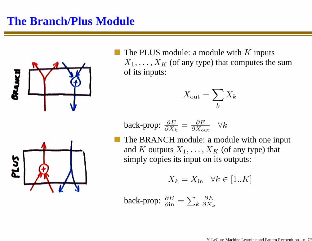
The Branch/Plus Module

The PLUS module: a module withK inputsX1, . . . , XK (of any type) that computes the sumof its inputs:

Xout =∑

k

Xk

back-prop: ∂E∂Xk

= ∂E∂Xout

∀k

The BRANCH module: a module with one inputandK outputsX1, . . . , XK (of any type) thatsimply copies its input on its outputs:

Xk = Xin ∀k ∈ [1..K]

back-prop:∂E∂in =

∑k

∂E∂Xk


The Switch Module

A module withK inputsX1, . . . , XK (ofany type) and one additionaldiscrete-valued inputY .

The value of the discrete input determineswhich of theN inputs is copied to theoutput.

Xout =∑

k

δ(Y − k)Xk

∂E

∂Xk

= δ(Y − k)∂E

∂Xout

the gradient with respect to the output iscopied to the gradient with respect to theswitched-in input. The gradients of all otherinputs are zero.


The Logsum Module

fprop:

Xout = −1

βlog

∑

k

exp(−βXk)

bprop:∂E

∂Xk

=∂E

∂Xout

exp(−βXk)∑j exp(−βXj)

or∂E

∂Xk

=∂E

∂XoutPk

with

Pk =exp(−βXk)∑j exp(−βXj)


Log-Likelihood Loss function and Logsum Modules

MAP/MLE LossLll(W, Y i, Xi) = E(W, Y i, Xi) + 1β

log∑

k exp(−βE(W, k, Xi))

A classifier trained with theLog-Likelihood loss can betransformed into an equivalentmachine trained with the energyloss.

The transformed machine containsmultiple “replicas” of the classifier,one replica for the desired output,andK replicas for each possiblevalue ofY .


Softmax Module

A single vector as input, and a “normalized” vector as output:

(Xout)i =exp(−βxi)∑k exp(−βxk)

Exercise: find the bprop∂(Xout)i

∂xj

=???


Radial Basis Function Network (RBF Net)

Linearly combined Gaussianbumps.

F (X, W, U) =∑i ui exp(−ki(X −Wi)

2)

The centers of the bumps can beinitialized with the K-meansalgorithm (see below), andsubsequently adjusted with gradientdescent.

This is a good architecture for re-gression and function approxima-tion.


MAP/MLE Loss and Cross-Entropy

classification (y is scalar and discrete). Let’s denoteE(y, X, W ) = Ey(X, W )

MAP/MLE Loss Function:

L(W ) =1

P

P∑

i=1

[Eyi(Xi, W ) +1

βlog

∑

k

exp(−βEk(Xi, W ))]

This loss can be written as

L(W ) =1

P

P∑

i=1

−1

βlog

exp(−βEyi(Xi, W ))∑k exp(−βEk(Xi, W ))


Cross-Entropy and KL-Divergence

let’s denoteP (j|Xi, W ) =exp(−βEj(X

i,W ))P

kexp(−βEk(Xi,W )) , then

L(W ) =1

P

P∑

i=1

1

βlog

1

P (yi|Xi, W )

L(W ) =1

P

P∑

i=1

1

β

∑

k

Dk(yi) logDk(yi)

P (k|Xi, W )

with Dk(yi) = 1 iff k = yi, and0 otherwise.

example1:D = (0, 0, 1, 0) andP (.|Xi, W ) = (0.1, 0.1, 0.7, 0.1). with β = 1,Li(W ) = log(1/0.7) = 0.3567

example2:D = (0, 0, 1, 0) andP (.|Xi, W ) = (0, 0, 1, 0). with β = 1,Li(W ) = log(1/1) = 0


Cross-Entropy and KL-Divergence

L(W ) =1

P

P∑

i=1

1

β

∑

k

Dk(yi) logDk(yi)

P (k|Xi, W )

L(W ) is proportional to thecross-entropy between the conditional distributionof y given by the machineP (k|Xi, W ) and thedesired distribution over classesfor samplei, Dk(yi) (equal to 1 for the desired class, and 0 for the otherclasses).

The cross-entropy also calledKullback-Leibler divergence between twodistributionsQ(k) andP (k) is defined as:

∑

k

Q(k) logQ(k)

P (k)

It measures a sort of dissimilarity between two distributions.

the KL-divergence is not a distance, because it is not symmetric, and it does notsatisfy the triangular inequality.


Multiclass Classification and KL-Divergence

Assume that our discriminant moduleF (X, W )produces a vector of energies, with one energyEk(X, W ) for each class.

A switch module selects the smallestEk to performthe classification.

As shown above, the MAP/MLE loss below be seenas a KL-divergence between the desired distributionfor y, and the distribution produced by the machine.

L(W ) =1

P

P∑

i=1

[Eyi(Xi, W )+1

βlog

∑

k

exp(−βEk(Xi, W ))]


Multiclass Classification and Softmax

The previous machine: discriminant function with oneoutput per class + switch, with MAP/MLE loss

It is equivalent to the following machine: discriminantfunction with one output per class + softmax + switch+ log loss

L(W ) =1

P

P∑

i=1

1

β− log P (yi|X, W )

with P (j|Xi, W ) =exp(−βEj(X

i,W ))P

kexp(−βEk(Xi,W )) (softmax of

the−Ej ’s).

Machines can be transformed into various equivalentforms to factorize the computation in advantageousways.


Multiclass Classification with a Junk Category

Sometimes, one of the categories is “none of the above”, how can we handlethat?

We add an extra energy wireE0 for the “junk” category which does not dependon the input.E0 can be a hand-chosen constant or can be equal to a trainableparameter (let’s call itw0).

everything else is the same.


NN-RBF Hybrids

sigmoid units are generally moreappropriate for low-level featureextraction.

Euclidean/RBF units are generally moreappropriate for final classifications,particularly if there are many classes.

Hybrid architecture for multiclass classifi-cation: sigmoids below, RBFs on top + soft-max + log loss.


Parameter-Space Transforms

Reparameterizing the function by transforming the space

E(Y, X, W )→ E(Y, X, G(U))

gradient descent inU space:

U ← U − η ∂G∂U

′ ∂E(Y,X,W )∂W

′

equivalent to the following algorithm inW

space:W ←W − η ∂G∂U

∂G∂U

′ ∂E(Y,X,W )∂W

′

dimensions:[Nw ×Nu][Nu ×Nw][Nw]


Parameter-Space Transforms: Weight Sharing

A single parameter is replicated multipletimes in a machine

E(Y, X, w1, . . . , wi, . . . , wj , . . .)→

E(Y, X, w1, . . . , uk, . . . , uk, . . .)

gradient:∂E()∂uk

= ∂E()∂wi

+ ∂E()∂wj

wi and wj are tied, or equivalently,uk isshared between two locations.


Parameter Sharing between Replicas

We have seen this before: a parameter controlsseveral replicas of a machine.

E(Y1, Y2, X, W ) = E1(Y1, X, W )+E1(Y2, X, W )

gradient:∂E(Y1,Y2,X,W )

∂W= ∂E1(Y1,X,W )

∂W+ ∂E1(Y2,X,W )

∂W

W is shared between two (or more) instances ofthe machine: just sum up the gradient contribu-tions from each instance.


Path Summation (Path Integral)

One variable influences the output through several others

E(Y, X, W ) =E(Y, F1(X, W ), F2(X, W ), F3(X, W ), V )

gradient:∂E(Y,X,W )∂X

=∑

i∂Ei(Y,Si,V )

∂Si

∂Fi(X,W )∂X

gradient:∂E(Y,X,W )∂W

=∑

i∂Ei(Y,Si,V )

∂Si

∂Fi(X,W )∂W

there is no need to implement these rules ex-plicitely. They come out naturally of the object-oriented implementation.


Mixtures of Experts

Sometimes, the function to be learned is consistent in restricted domains of the inputspace, but globally inconsistent.Example: piecewise linearly separable function.

Solution: a machine composed of several“experts” that are specialized on subdomains ofthe input space.

The output is a weighted combination of theoutputs of each expert. The weights are producedby a “gater” network that identifies whichsubdomain the input vector is in.

F (X, W ) =∑

k ukF k(X, W k) with

uk = exp(−βGk(X,W 0))P

kexp(−βGk(X,W 0))

the expert weightsuk are obtained by softmax-ingthe outputs of the gater.

example: the two experts are linear regressors, thegater is a logistic regressor.


Sequence Processing: Time-Delayed Inputs

The input is a sequence of vectorsXt.

simple idea: the machine takes a timewindow as input

R = F (Xt, Xt−1, Xt−2, W )

Examples of use:predict the next sample in a timeseries (e.g. stock market, waterconsumption)predict the next character or word in atextclassify an intron/exon transition in aDNA sequence


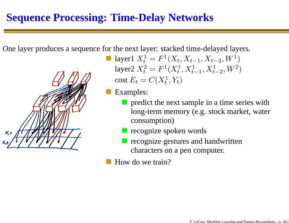
Sequence Processing: Time-Delay Networks

One layer produces a sequence for the next layer: stacked time-delayed layers.layer1X1

t = F 1(Xt, Xt−1, Xt−2, W1)

layer2X2t = F 1(X1

t , X1t−1, X

1t−2, W

2)

costEt = C(X1t , Yt)

Examples:predict the next sample in a time series withlong-term memory (e.g. stock market, waterconsumption)recognize spoken wordsrecognize gestures and handwrittencharacters on a pen computer.

How do we train?


Training a TDNN

Idea: isolate the minimal network that influences the energyat one particular time stept.

in our example, this is influenced by 5 timesteps on the input.

train this network in isolation, taking those5 time steps as the input.

Surprise: we have three identical replicasof the first layer units that share the sameweights.

We know how to deal with that.

do the regular backprop, and add up thecontributions to the gradient from the 3replicas


Convolutional Module

If the first layer is a set of linear units with sigmoids, we canview it as performing asort ofmultiple discrete convolutions of the input sequence.

1D convolution operation:

S1t =

∑Tj=1 W 1

j

′

Xt−j .

wjk j ∈ [1, T ] is aconvolution kernel

sigmoidX1t = tanh(S1

t )

derivative: ∂E∂w1

jk

=∑3

t=1∂E∂S1

t

Xt−j


Simple Recurrent Machines

The output of a machine is fed back to some of its inputsZ. Zt+1 = F (Xt, Zt, W ),wheret is a time index. The inputX is not just a vector but a sequence of vectorsXt.

This machine is adynamical system withan internal stateZt.

Hidden Markov Models are a special caseof recurrent machines whereF is linear.


Unfolded Recurrent Nets and Backprop through time

To train a recurrent net: “unfold” it in timeand turn it into a feed-forward net with asmany layers as there are time steps in theinput sequence.

An unfolded recurrent net is a very “deep”machine where all the layers are identicaland share the same weights.

∂E∂W

=∑

t∂E∂Zt

∂F (Xt,Zt,W )∂W

This method is calledback-propagationthrough time.

examples of use: process control (steel mill,chemical plant, pollution control....), robotcontrol, dynamical system modelling...


other topologies - computational intelligence, learning

Documents