Other-regarding Preferences, In-group Bias and Political

Participation: an Experiment

ABSTRACT

This paper presents an experimental study on the relationship between other-regarding

preferences, in-group bias and political participation. We conjecture that subjects who are more

other-regarding and exhibit higher in-group bias are more likely to bear the costs of participating

in group action. Using a participation game, we implement laboratory elections in which two

groups compete for victory. We induce different levels of in-group bias across subjects in order

to implement treatments in which the competing groups are either highly biased towards the

own group vis-à-vis the other one or are characterized by low levels of such in-group bias. Our

results show that, at the aggregate level, participation is higher in environments where in-group

bias is more pronounced. Furthermore, the least other-regarding subjects participate much less

often that others, while the more other-regarding sustain high participation levels. These

findings suggest that interpersonal preferences and intergroup bonds can explain the higher

participation of close-knit (political) groups observed in the field.

KEYWORDS: In-group bias, Other-regarding preferences, Political participation, Participation

Game, Experiment.

1

1. Introduction In many modern societies, conflicts of interest center around groups (e.g., workers versus

capital owners or Democrats versus Republicans). Such group conflicts can be solved through

democratic politics. A group’s success in the political arena depends on many factors, however.

One important element is the extent to which its members participate in its political endeavors.

Often, the group with the highest level of participation is most likely to be politically successful,

and therefore has a high probability of success in conflicts with other groups.

The importance of groups in the political arena has been widely recognized. In his appraisal

of the rational choice literature on election participation, Feddersen (2004) argues that "while a

canonical model does not yet exist, the literature appears to be converging toward a ‘group-

based’ model of turnout, in which group members participate in elections either because they

are directly coordinated and rewarded by leaders as in ‘mobilization’ models or because they

believe themselves to be ethically obliged to act in a manner that is consistent with the group's

interest as in ‘ethical agent’ models." It is to this literature on the role of groups in politics that

our paper aims to contribute.

In particular, this paper studies political participation in the context of groups competing

for benefits. We address the question of how this participation is affected by the interaction

between, on the one hand, a sense of in-group bias that members may have and, on the other

hand, the extent to which members have preferences that take into account the well-being of

others. A higher sense of in-group bias typically results in favoritism towards its members and a

discrimination of the out-group’s members.

Individuals facing the decision of whether to participate in group action typically experience

a social dilemma towards their group, i.e., a situation in which the members of the in-group

would be better off if all participated, but where individual incentives make non-participation

more attractive (Dawes, 1980). The social dilemma situations we are interested in involve a

conflict with other groups. A prime example is an election where two factions of an electorate

compete for victory: the group with higher participation wins the election and reaps the

benefits. In this environment, free-riding is often an equilibrium strategy if individuals are

perfectly rational and have self-interested preferences (Palfrey and Rosenthal 1983). However,

relaxing either of these postulates can account for participation, as in the group-based turnout

models of Morton (1991), Schram and van Winden (1991) and Shachar and Nalebuff (1999).

Investigating the relationship between participation and in-group bias is important because

the outcome of group conflicts can have severe consequences for the members of the groups

concerned, irrespective of an individual member's decision to participate in it. If certain

individuals or groups participate more than others, this might bias policy in a direction that is

not representative of the majority's preferences. If, for example, some groups manage to create

a stronger feeling of in-group favoritism than others, this could put them in an advantageous

position that is unrelated to the conflict at hand. Either of these effects could harm the efficient

use of an economy's resources because they yield an allocation that is biased towards the

preferences of the political participators (see Lijphart 1997 for a similar argument with respect

to election turnout).

We conjecture that the individual participation decision in group effort takes into account

the ties that bind the group together. Moreover, an individual may more generally take the

2

consequences for others into account when deciding on her actions. In other words, an

individual may have other-regarding preferences. Other-regarding preferences, as we use the

term, are those that include motives related to the well-being of others, as opposed to selfish

or self-regarding preferences (Sen 1977). However, other-regarding preferences might

discriminate between in-group and out-group members, and how much an individual cares for

each is likely to influence the sacrifices she is willing to make. Our paper addresses this

conjecture by studying the effect of other-regarding preferences and in-group bias on

participation in group action.

An important goal of our experimental design is therefore to create environments with

distinct levels of in-group bias in order to study its influence on individual and aggregate

participation. In addition, we want to know whether participation depends on other-regarding

motivations, both in general and in interaction with in-group bias. For this purpose, the design

includes a measurement of such motivations, using a so-called value orientation test. Finally, we

measure political participation by studying individual choices in a participation game (Palfrey

and Rosenthal 1983): two groups of equal size compete for benefits and the winning group is

the one with highest participation. Hence, our experiment induces distinct levels of in-group

bias, measures other-regarding preferences and allows us to link (combinations of) these

variables to political participation.

In order to derive hypotheses on individual and aggregate behavior, we combine insights

from a theoretical analysis of the participation game with the available empirical evidence. First,

we hypothesize that other-regarding subjects will participate more often than those who are

selfish. Second, we expect environments with a high bias towards the in-group to foster fiercer

competition, and therefore generate higher aggregate participation. Third, we hypothesize that

subjects who exhibit larger bias towards their group will participate more often.

Our results may be summarized as follows. First, they provide support for the hypothesis

that individual participation is higher for other-regarding subjects. In particular, we observe that

the most uncooperative subjects stand out from the rest by abstaining much more often. The

estimated model predicts a 50 percentage point-difference in participation between the most

selfish and the most other-regarding subjects. Second, we were successful in inducing distinct

levels of in-group bias across treatments. This allows us to conclude that aggregate participation

is higher in environments where in-group bias is high, albeit modestly. Third, individuals who

have a higher degree of in-group bias in the first place participate more often. Our experimental

inducement of further in-group bias crowds out this relationship, however.

To the best of our knowledge, our laboratory study is the first to measure other-regarding

preferences and induce different levels of in-group bias in the context of a political participation

game.1 Our results are an indication that both other-regarding preferences and in-group bias

matter. Though groups may not be able to affect their members’ preferences, the latter result

does suggest that groups that manage to increase their members’ bias towards the group will

fare relatively well in conflicts with other groups.

The organization of this paper is as follows. The next section discusses the literature that

relates political participation to other-regarding preferences and in-group bias. Section 3

presents the conceptual analysis of the participation game and our hypotheses. Section 4

1 Rabbie and Wilkins (1971), Bornstein et al. (2002), and Reichmann and Weimann (2008) investigate group competition in environments where group identity may play a role, but do not explicitly study the effects of this in-group bias. They also do not compare environments that vary in the extent to which in-group bias has been induced.

3

describes the experimental design. In section 5, we present and analyze our data. A final section

concludes.

2. Related Literature Both other-regarding preferences and group identity have been the subject of recent

attention within the rational choice approach to political participation. This approach has

traditionally struggled with the so-called ‘paradox of participation’: the fact that the high rates

of participation observed empirically (e.g., in large-scale elections) are at odds with the

theoretical observation that participation is seemingly irrational. For a survey of the literature

in economics, political science and related disciplines, see, e.g., Aldrich (1997), Blais (2000),

Dhillon and Peralta (2000), or Feddersen (2004).

Notwithstanding, many works in this research paradigm have by now uncovered various

factors that help explain why rational individuals may participate in group action (see Palfrey

2009 for an overview). In particular, the addition of other-regarding preferences to the calculus

of participation has led to models that escape the prediction of low participation. For individuals

with such preferences, participation becomes instrumentally rational if the benefits derived

from one's group winning (which now include the benefits to co-members) are not overcome

by the low probability of being pivotal. Models in this vein have been proposed by Jankowski

(2002), Edlin et al. (2007), Feddersen et al. (2009), and Evren (2012). There is both field (Knack

1992, Jankowski 2007) and experimental (Fowler 2006, Fowler and Kam 2007, Dawes et al. 2011)

evidence supporting a positive relationship between social preferences and participation.

Our results add to this stream of literature by relating a direct measure of an individual's

level of other-regarding preferences to the frequency of participation in intergroup competition.

Moreover, we contribute with novel evidence on the interaction between an individual's other-

regarding concerns and the extent to which she is biased towards her own group relative to the

other group. To some extent, this analysis supplements the work conducted by Fowler (2006),

who uses a combination of field and experimental data to show that social identity (proxied by

party identification) amplifies the positive impact of altruistic motivations on political

participation. Though the first to combine other-regarding preferences and group identity,

Fowler’s methodology has some shortcomings related to the lack of control in the field.2 Our

laboratory control allows us to measure other-regarding preferences and induce in-group bias

in ways that rule out priming and response bias effects that are likely to occur in a situation

where measurements are based on politically framed survey questions.

The empirical literature on the socio-economic determinants of participation (e.g., the

seminal work by Verba and Nie 1972) has established a number of important relationships, such

as a positive correlation between income and participation. However, some puzzles remain. For

example, the positive correlation between income, education, and participation is much weaker

for African-American voters, who participate beyond what their socioeconomic status would

predict. Leighley and Vedlitz (1999) provide a number of candidate explanations for this

2 Fowler uses survey questions regarding election participation, party identification, and political knowledge. Subsequently, subjects play a dictator game, either against someone with the same political preference, a different political preference or an unknown preference. These dictator choices are poorly incentivized, however. The observed distribution of giving is at odds with recent meta-studies (Engel 2011), but in line with non-incentivized studies. His results show that more altruistic individuals do not participate more unless they are strong party identifiers.

4

phenomenon: psychological resources (e.g., political interest and participation efficacy beliefs),

social connectedness, and group identity. All of these explanations have a theoretical basis but

it is difficult to identify in the field which mechanisms are at work. For example, it is hard to

disentangle the effect of group identity from the impact of social connectedness on

participation. Do the members of a group voluntarily participate because of their strong sense

of group identity, or because their environment encourages participation?

This example shows how difficult it is to isolate the effects of group membership on the

participation decision. Furthermore, social context, social networks, and participation behavior

are endogenously determined, making it difficult to elicit the direction of causality. In contrast,

an easy and clean test of the in-group bias effect can be obtained in the controlled laboratory

environment. By comparing the behavior of groups that differ only with respect to their bias

toward the in-group, we can isolate the effect of in-group bias on participation.

The so-called group identity paradigm studies the influence of ‘group-belonging'

sentiments on how individuals make decisions in instances of intergroup behavior (Tajfel 1982,

Hogg and Abrams 1988, Ellemers 2012). The body of knowledge on group identity that has

developed over the past few decades is quite extensive and has produced a number of robust

findings (see Brewer 2007, Eckel and Grossman 2005). Experimental studies have shown that

group identity and its salience impacts strategic behavior (Charness et al. 2007) and that

individuals tend to be more altruistic towards in-group members (Chen and Li 2009), for

example.

As many other papers in this literature (e.g., Eckel and Grossman, Chen and Li 2009), we

induce different levels of in-group bias by resorting to procedures that combine minimal group

assignment with further manipulations (e.g., communication or team-building tasks). These

manipulations aim at generating a strong group identification process through an increase in the

salience of the in-group and the out-group. From this increased identification with the in-group

we expect to observe high levels of in-group bias, which ultimately is the variable we measure

and control in this study. As mentioned, we conjecture that stronger in-group bias will be

associated with more frequent participation in group action. Using observational data, Simon et

al. (1998) and Stürmer and Simon (2004), among others, have indeed shown that the willingness

to participate in group action is significantly related to collective identification processes.

3. Conceptual Framework and Hypotheses We study participation behavior using the game proposed by Palfrey and Rosenthal (1983).

This section provides an outline of this framework and the main results that follow from our

implementation (Appendix A presents a more formal analysis).

Two groups of equal size compete for victory, which depends on participation. Each player

decides simultaneously and privately whether or not to participate at a cost (c). The group where

more players participate wins. Players on the winning side obtain a monetary payoff (BW) that is

higher than the one accruing to players on the losing side (BL). In case of a tie, the winner is

decided by a fair coin toss. The structure and payoffs of the game are common knowledge.

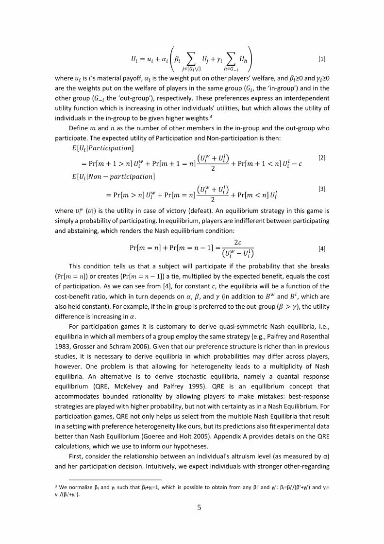
We assume that players have a utility function that allows for other-regarding (or

‘altruistic’, a term we use interchangeably) and group-discriminating components:

5

𝑈𝑖 = 𝑢𝑖 + 𝛼𝑖 (𝛽𝑖 ∑ 𝑈𝑗 +

𝑗∊𝐺𝑖\𝑖

𝛾𝑖 ∑ 𝑈ℎ

ℎ∊𝐺−𝑖

) [1]

where 𝑢𝑖 is 𝑖’s material payoff, 𝛼𝑖 is the weight put on other players’ welfare, and 𝛽𝑖≥0 and 𝛾𝑖≥0

are the weights put on the welfare of players in the same group (𝐺𝑖, the ‘in-group’) and in the

other group (𝐺−𝑖 the ‘out-group’), respectively. These preferences express an interdependent

utility function which is increasing in other individuals' utilities, but which allows the utility of

individuals in the in-group to be given higher weights.3

Define 𝑚 and 𝑛 as the number of other members in the in-group and the out-group who

participate. The expected utility of Participation and Non-participation is then:

𝐸[𝑈𝑖|𝑃𝑎𝑟𝑡𝑖𝑐𝑖𝑝𝑎𝑡𝑖𝑜𝑛]

= Pr[𝑚 + 1 > 𝑛]𝑈𝑖𝑤 + Pr[𝑚 + 1 = 𝑛]

(𝑈𝑖𝑤 + 𝑈𝑖

𝑙)

2+ Pr[𝑚 + 1 < 𝑛]𝑈𝑖

𝑙 − 𝑐

[2]

𝐸[𝑈𝑖|𝑁𝑜𝑛 − 𝑝𝑎𝑟𝑡𝑖𝑐𝑖𝑝𝑎𝑡𝑖𝑜𝑛]

= Pr[𝑚 > 𝑛]𝑈𝑖𝑤 + Pr[𝑚 = 𝑛]

(𝑈𝑖𝑤 + 𝑈𝑖

𝑙)

2+ Pr[𝑚 < 𝑛]𝑈𝑖

𝑙 [3]

where 𝑈𝑖𝑤 (𝑈𝑖

𝑙) is the utility in case of victory (defeat). An equilibrium strategy in this game is

simply a probability of participating. In equilibrium, players are indifferent between participating

and abstaining, which renders the Nash equilibrium condition:

Pr[𝑚 = 𝑛] + Pr[𝑚 = 𝑛 − 1] =

2𝑐

(𝑈𝑖𝑤 − 𝑈𝑖

𝑙) [4]

This condition tells us that a subject will participate if the probability that she breaks

(Pr[𝑚 = 𝑛]) or creates (Pr[𝑚 = 𝑛 − 1]) a tie, multiplied by the expected benefit, equals the cost

of participation. As we can see from [4], for constant c, the equilibria will be a function of the

cost-benefit ratio, which in turn depends on 𝛼, 𝛽, and 𝛾 (in addition to 𝐵𝑤 and 𝐵𝑙, which are

also held constant). For example, if the in-group is preferred to the out-group (𝛽 > 𝛾), the utility

difference is increasing in 𝛼.

For participation games it is customary to derive quasi-symmetric Nash equilibria, i.e.,

equilibria in which all members of a group employ the same strategy (e.g., Palfrey and Rosenthal

1983, Grosser and Schram 2006). Given that our preference structure is richer than in previous

studies, it is necessary to derive equilibria in which probabilities may differ across players,

however. One problem is that allowing for heterogeneity leads to a multiplicity of Nash

equilibria. An alternative is to derive stochastic equilibria, namely a quantal response

equilibrium (QRE, McKelvey and Palfrey 1995). QRE is an equilibrium concept that

accommodates bounded rationality by allowing players to make mistakes: best-response

strategies are played with higher probability, but not with certainty as in a Nash Equilibrium. For

participation games, QRE not only helps us select from the multiple Nash Equilibria that result

in a setting with preference heterogeneity like ours, but its predictions also fit experimental data

better than Nash Equilibrium (Goeree and Holt 2005). Appendix A provides details on the QRE

calculations, which we use to inform our hypotheses.

First, consider the relationship between an individual's altruism level (as measured by α)

and her participation decision. Intuitively, we expect individuals with stronger other-regarding

3 We normalize βi and γi such that βi+γi=1, which is possible to obtain from any βi′ and γi′: βi=βi'/(β'+γi') and γi= γi'/(βi'+γi').

6

preferences to be more willing to sacrifice themselves for their group, provided they prefer the

in-group to the out-group (a weak assumption). This is another way of saying that there is more

at stake for an individual who values the welfare of others in her group, and therefore stronger

other-regarding preferences will lead to more frequent participation. The theoretical analysis of

the game indeed provides evidence that the (quantal response) equilibrium level of participation

is increasing in other-regarding concerns (α) in a broad parameter range, including parameters

that are compatible with, and estimated from, our data (cf. Appendix A). The existing empirical

evidence provides further support for the conjecture that other-regarding concerns foster

individual participation. Relating self-stated motivations to participation game behavior, Schram

and Sonnemans (1996b) found that subjects with individualistic goals were less likely to

participate, whereas subjects with cooperative goals were more likely to participate.4 Hence,

our equilibrium analysis and previous evidence both point to a positive effect of altruism on

participation (i.e., altruism is in-group targeting). This yields our first hypothesis:

Hypothesis 1: Individual participation is increasing in the level of other-regarding concerns,

i.e., more altruistic subjects participate at higher rates.

Next, we consider the effects of in-group bias on participation. We are mainly concerned

whether participation is higher when in-group bias is more pronounced. The QRE that we obtain

show that aggregate participation is increasing in in-group bias levels. This is supported by the

empirical regularities mentioned in the previous section, in particular the fact that in-group

favoritism leads to more competitive behavior. We therefore expect higher aggregate

participation when in-group bias is induced. In line with this conjecture, Schram and Sonnemans

(1996b) study the effect of group identity on participation behavior by implementing different

matching protocols in a participation game.5 They elicit group identity using the minimal group

paradigm and find that the effect of group identity is significant, though not pronounced.

Moreover, various studies using the participation game framework (Bornstein et al. 1989,

Bornstein 1992, Schram and Sonnemans 1996a,b, Goren and Bornstein 2000) explore

experimentally the role of communication within the in-group. Several papers show that the

exchange of non-binding promises (cheap talk) between group members reinforces the sense of

group identity (e.g., Chen and Li, 2009). In participation game experiments, such communication

significantly increases participation levels.6 This allows us to formulate our second hypothesis:

Hypothesis 2a: Higher in-group bias leads to higher levels of aggregate participation.

4 In fact, this is precisely what experimental subjects will tell you. The post-experiment questionnaire asked subjects what they thought moved a participant who participated often. More than 70% responded that this was either cooperation towards the in-group or cooperation towards both groups. Moreover, a participant who participated rarely was attributed a selfish motivation by 77.5% of the subjects. For details, see Table C 1 in the Appendix. 5 Schram and Sonnemans (1996b) implement three treatment conditions which were conceived to yield increasing levels of group identity: i) group composition varied from period to period, and both subject identity and choices were anonymous; ii) group composition remained constant, and both identity and choices were anonymous; iii) group composition remained constant, identity was revealed, but choices remained anonymous. Participation in ii) was higher than in i), but also higher than in iii). 6 Goren and Bornstein (2000) show that without communication players associate high participation levels to cooperation towards the in-group and do not associate low levels of participation to inter-group cooperation.

7

We further consider situations where individuals within groups are heterogeneous in terms

of their in-group bias, which allows us to address how it operates at the individual level. Do

subjects with a higher level of in-group bias participate more often than subjects with lower

levels of in-group bias? The theoretical results show that subjects with a higher in-group bias

will tend to participate with a higher probability in a relevant parameter range. Intuitively, the

reason may be that individuals who identify more with their group are more willing to incur

sacrifices for it, and therefore participate at higher rates. Our third hypothesis follows:

Hypothesis 2b: Subjects with a higher sense of in-group bias participate at higher rates.

4. Experimental Design Our experiment is composed of three main parts, each to be explained in detail below.7 In

the first part, we measure the subjects' other-regarding preferences. In the second part, we vary

the group formation procedure in order to obtain environments where in-group bias is either

high or low. Allocation decisions and survey questions are used to measure the degree of in-

group bias. In the third part, subjects interact in the participation game (Palfrey and Rosenthal

1983) explained in the previous section. See Figure 1 for a diagram showing the sequence of

these parts throughout an experimental session.

Figure 1 - Sequence in the Experiment.

Notes. Solid lines indicate the sequence in the High and Low treatments, while

dashed lines indicate the sequence in the Control treatment. BFI: Big Five

Inventory.

The sessions were run at the CREED laboratory of the University of Amsterdam (UvA).

Participants were recruited from the CREED laboratory subject pool using the laboratory’s online

registration system. The subject pool consists of approximately 2000 students, mainly UvA

undergraduates from various disciplines. A total of 160 subjects (44% of which were female)

participated in 8 sessions (with 20 subjects each), which took place in June and October 2011.

On average, participants earned 28.5 Euros, which included a 7 Euro show-up fee. The

experiment was programmed and conducted in z-Tree (Fischbacher 2007). Payoffs in the

experiment were expressed in tokens, exchanged to Euros at a rate of 0.005 Euros per token.

For the first and third parts (ring test and participation game), we administered practice

questions before each part to check subject understanding. The typical experimental session

lasted around two hours. All procedures within a session were known to participants.

7 See Appendix E for a transcript of the instructions.

8

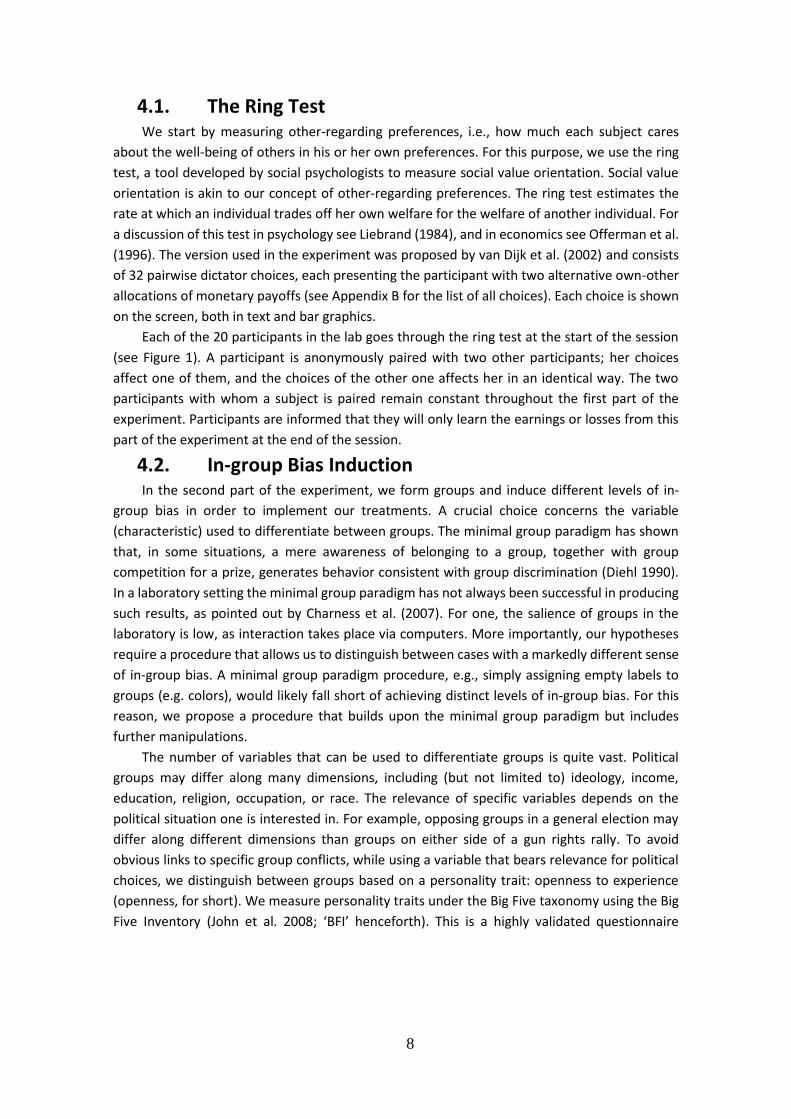
4.1. The Ring Test We start by measuring other-regarding preferences, i.e., how much each subject cares

about the well-being of others in his or her own preferences. For this purpose, we use the ring

test, a tool developed by social psychologists to measure social value orientation. Social value

orientation is akin to our concept of other-regarding preferences. The ring test estimates the

rate at which an individual trades off her own welfare for the welfare of another individual. For

a discussion of this test in psychology see Liebrand (1984), and in economics see Offerman et al.

(1996). The version used in the experiment was proposed by van Dijk et al. (2002) and consists

of 32 pairwise dictator choices, each presenting the participant with two alternative own-other

allocations of monetary payoffs (see Appendix B for the list of all choices). Each choice is shown

on the screen, both in text and bar graphics.

Each of the 20 participants in the lab goes through the ring test at the start of the session

(see Figure 1). A participant is anonymously paired with two other participants; her choices

affect one of them, and the choices of the other one affects her in an identical way. The two

participants with whom a subject is paired remain constant throughout the first part of the

experiment. Participants are informed that they will only learn the earnings or losses from this

part of the experiment at the end of the session.

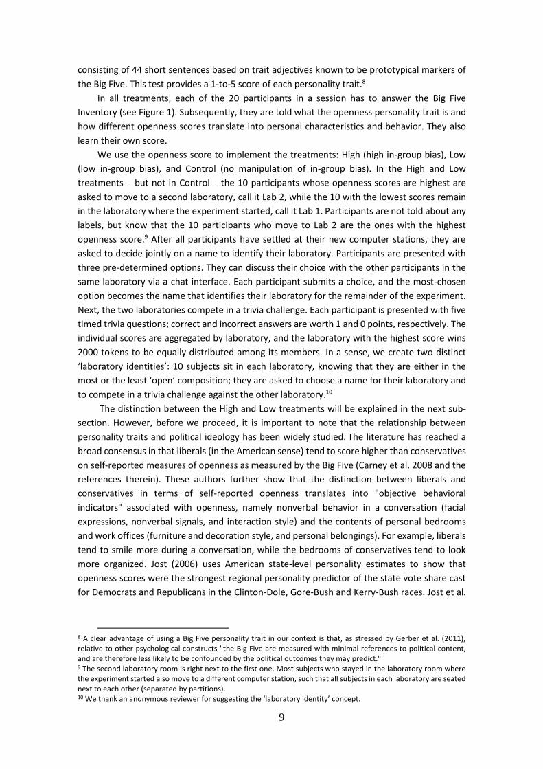
4.2. In-group Bias Induction In the second part of the experiment, we form groups and induce different levels of in-

group bias in order to implement our treatments. A crucial choice concerns the variable

(characteristic) used to differentiate between groups. The minimal group paradigm has shown

that, in some situations, a mere awareness of belonging to a group, together with group

competition for a prize, generates behavior consistent with group discrimination (Diehl 1990).

In a laboratory setting the minimal group paradigm has not always been successful in producing

such results, as pointed out by Charness et al. (2007). For one, the salience of groups in the

laboratory is low, as interaction takes place via computers. More importantly, our hypotheses

require a procedure that allows us to distinguish between cases with a markedly different sense

of in-group bias. A minimal group paradigm procedure, e.g., simply assigning empty labels to

groups (e.g. colors), would likely fall short of achieving distinct levels of in-group bias. For this

reason, we propose a procedure that builds upon the minimal group paradigm but includes

further manipulations.

The number of variables that can be used to differentiate groups is quite vast. Political

groups may differ along many dimensions, including (but not limited to) ideology, income,

education, religion, occupation, or race. The relevance of specific variables depends on the

political situation one is interested in. For example, opposing groups in a general election may

differ along different dimensions than groups on either side of a gun rights rally. To avoid

obvious links to specific group conflicts, while using a variable that bears relevance for political

choices, we distinguish between groups based on a personality trait: openness to experience

(openness, for short). We measure personality traits under the Big Five taxonomy using the Big

Five Inventory (John et al. 2008; ‘BFI’ henceforth). This is a highly validated questionnaire

9

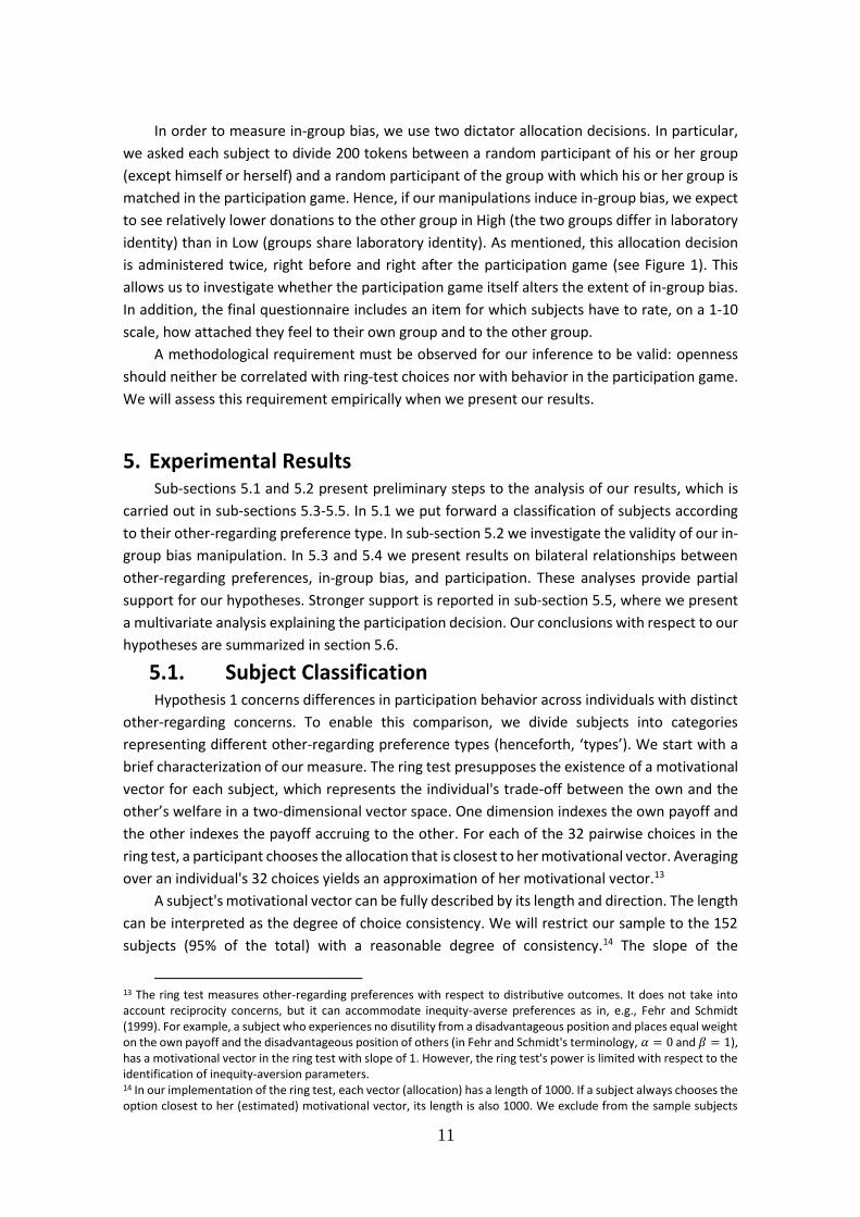
consisting of 44 short sentences based on trait adjectives known to be prototypical markers of

the Big Five. This test provides a 1-to-5 score of each personality trait.8

In all treatments, each of the 20 participants in a session has to answer the Big Five

Inventory (see Figure 1). Subsequently, they are told what the openness personality trait is and

how different openness scores translate into personal characteristics and behavior. They also

learn their own score.

We use the openness score to implement the treatments: High (high in-group bias), Low

(low in-group bias), and Control (no manipulation of in-group bias). In the High and Low

treatments – but not in Control – the 10 participants whose openness scores are highest are

asked to move to a second laboratory, call it Lab 2, while the 10 with the lowest scores remain

in the laboratory where the experiment started, call it Lab 1. Participants are not told about any

labels, but know that the 10 participants who move to Lab 2 are the ones with the highest

openness score.9 After all participants have settled at their new computer stations, they are

asked to decide jointly on a name to identify their laboratory. Participants are presented with

three pre-determined options. They can discuss their choice with the other participants in the

same laboratory via a chat interface. Each participant submits a choice, and the most-chosen

option becomes the name that identifies their laboratory for the remainder of the experiment.

Next, the two laboratories compete in a trivia challenge. Each participant is presented with five

timed trivia questions; correct and incorrect answers are worth 1 and 0 points, respectively. The

individual scores are aggregated by laboratory, and the laboratory with the highest score wins

2000 tokens to be equally distributed among its members. In a sense, we create two distinct

‘laboratory identities’: 10 subjects sit in each laboratory, knowing that they are either in the

most or the least ‘open’ composition; they are asked to choose a name for their laboratory and

to compete in a trivia challenge against the other laboratory.10

The distinction between the High and Low treatments will be explained in the next sub-

section. However, before we proceed, it is important to note that the relationship between

personality traits and political ideology has been widely studied. The literature has reached a

broad consensus in that liberals (in the American sense) tend to score higher than conservatives

on self-reported measures of openness as measured by the Big Five (Carney et al. 2008 and the

references therein). These authors further show that the distinction between liberals and

conservatives in terms of self-reported openness translates into "objective behavioral

indicators" associated with openness, namely nonverbal behavior in a conversation (facial

expressions, nonverbal signals, and interaction style) and the contents of personal bedrooms

and work offices (furniture and decoration style, and personal belongings). For example, liberals

tend to smile more during a conversation, while the bedrooms of conservatives tend to look

more organized. Jost (2006) uses American state-level personality estimates to show that

openness scores were the strongest regional personality predictor of the state vote share cast

for Democrats and Republicans in the Clinton-Dole, Gore-Bush and Kerry-Bush races. Jost et al.

8 A clear advantage of using a Big Five personality trait in our context is that, as stressed by Gerber et al. (2011), relative to other psychological constructs "the Big Five are measured with minimal references to political content, and are therefore less likely to be confounded by the political outcomes they may predict." 9 The second laboratory room is right next to the first one. Most subjects who stayed in the laboratory room where the experiment started also move to a different computer station, such that all subjects in each laboratory are seated next to each other (separated by partitions). 10 We thank an anonymous reviewer for suggesting the ‘laboratory identity’ concept.

10

(2003) show that the relationship between openness and ideology extends to non-American

samples.

In sum, openness is one of the best proxies for ideological dispositions and has been shown

to matter for political choices, like party choice. However, openness does not affect participation

decisions.11 Groups with contrasting openness levels are thus composed of individuals who

would make different political choices, and therefore draw a parallel to what would distinguish

groups in many political conflicts. The obvious advantage of using a personality trait instead of

self-reported ideology is to avoid confounds implied by the meaning of ideology at a certain

point in time or within a particular party system.

4.3. Participation Game and Treatment Implementation For the participation game, subjects are allocated to groups of five participants, with two

groups constituting an ‘electorate’ of ten participants. The parameter values used throughout

the second part of the experiment are BW=120, BL=30, and c=30. Groups remain constant and

play the game for 40 rounds. At the end of each round, participants are informed of how many

others participated in each group, their own token earnings in that round, and their cumulative

token earnings in that part of the experiment.

The High and Low treatments differ with respect to the groups that interact in the

participation game (see Figure 2). Regardless of treatment, all members of the in-group belong

to the same laboratory. The difference lies in which laboratory the out-group is drawn from. In

the High treatment, the in-group and the out-group are drawn from different laboratories, i.e.,

they have different laboratory identities. In the Low treatment, both the in-group and the out-

group belong to the same laboratory, i.e., they share the same laboratory identity.

The Control treatment differs from High and Low in that the in-group bias induction does

not take place. Subjects in Control answer the BFI, receive feedback on their openness score,

and are then immediately matched into participation game groups. All 20 subjects remain in the

laboratory where the experiment started. Hence, subjects in the Control treatment do not know

that they are allocated to groups based on their openness score.12

Figure 2– Experimental treatments.

Notes: Arrows indicate competition in the Participation Game. ‘Ranking’ refers to

the openness score ranking. Group 1 is composed of subjects with rankings 1 to 5,

Group 2 with rankings 6 to 10, and so on.

11 Some studies have investigated the relationship between openness and political participation. There is no evidence of a robust causal relationship between openness and participation (Mondak et al.,2010). Similarly, Gerber et al. (2011) find no relationship between openness and recorded voter turnout. 12 The underlying group formation protocol in Control mimics High in terms of openness scores. That is, Group 1(2) competes with Group 3(4). Note that each group has the same openness score composition across treatments. Our empirical results show that openness does not influence participation (see sub-section 5.2), and therefore the matching protocol adopted in the Control sessions should not influence participation behavior.

11

In order to measure in-group bias, we use two dictator allocation decisions. In particular,

we asked each subject to divide 200 tokens between a random participant of his or her group

(except himself or herself) and a random participant of the group with which his or her group is

matched in the participation game. Hence, if our manipulations induce in-group bias, we expect

to see relatively lower donations to the other group in High (the two groups differ in laboratory

identity) than in Low (groups share laboratory identity). As mentioned, this allocation decision

is administered twice, right before and right after the participation game (see Figure 1). This

allows us to investigate whether the participation game itself alters the extent of in-group bias.

In addition, the final questionnaire includes an item for which subjects have to rate, on a 1-10

scale, how attached they feel to their own group and to the other group.

A methodological requirement must be observed for our inference to be valid: openness

should neither be correlated with ring-test choices nor with behavior in the participation game.

We will assess this requirement empirically when we present our results.

5. Experimental Results Sub-sections 5.1 and 5.2 present preliminary steps to the analysis of our results, which is

carried out in sub-sections 5.3-5.5. In 5.1 we put forward a classification of subjects according

to their other-regarding preference type. In sub-section 5.2 we investigate the validity of our in-

group bias manipulation. In 5.3 and 5.4 we present results on bilateral relationships between

other-regarding preferences, in-group bias, and participation. These analyses provide partial

support for our hypotheses. Stronger support is reported in sub-section 5.5, where we present

a multivariate analysis explaining the participation decision. Our conclusions with respect to our

hypotheses are summarized in section 5.6.

5.1. Subject Classification Hypothesis 1 concerns differences in participation behavior across individuals with distinct

other-regarding concerns. To enable this comparison, we divide subjects into categories

representing different other-regarding preference types (henceforth, ‘types’). We start with a

brief characterization of our measure. The ring test presupposes the existence of a motivational

vector for each subject, which represents the individual's trade-off between the own and the

other’s welfare in a two-dimensional vector space. One dimension indexes the own payoff and

the other indexes the payoff accruing to the other. For each of the 32 pairwise choices in the

ring test, a participant chooses the allocation that is closest to her motivational vector. Averaging

over an individual's 32 choices yields an approximation of her motivational vector.13

A subject's motivational vector can be fully described by its length and direction. The length

can be interpreted as the degree of choice consistency. We will restrict our sample to the 152

subjects (95% of the total) with a reasonable degree of consistency.14 The slope of the

13 The ring test measures other-regarding preferences with respect to distributive outcomes. It does not take into account reciprocity concerns, but it can accommodate inequity-averse preferences as in, e.g., Fehr and Schmidt (1999). For example, a subject who experiences no disutility from a disadvantageous position and places equal weight on the own payoff and the disadvantageous position of others (in Fehr and Schmidt's terminology, 𝛼 = 0 and 𝛽 = 1), has a motivational vector in the ring test with slope of 1. However, the ring test's power is limited with respect to the identification of inequity-aversion parameters. 14 In our implementation of the ring test, each vector (allocation) has a length of 1000. If a subject always chooses the option closest to her (estimated) motivational vector, its length is also 1000. We exclude from the sample subjects

12

motivational vector – which can also be expressed as the angle formed by the vector and the

horizontal axis – describes the trade-off between the own and the other’s welfare. For example,

one can think of an individual whose vector has an angle of 26.6° – corresponding to a slope of

0.5 – as someone willing to give away 50 Euro cents to another individual for each Euro she

keeps for herself. The slope of the vector provides a measure of α in Equation [1]: the marginal

rate of substitution of i’s utility of money for j’s utility. The average angle of the motivational

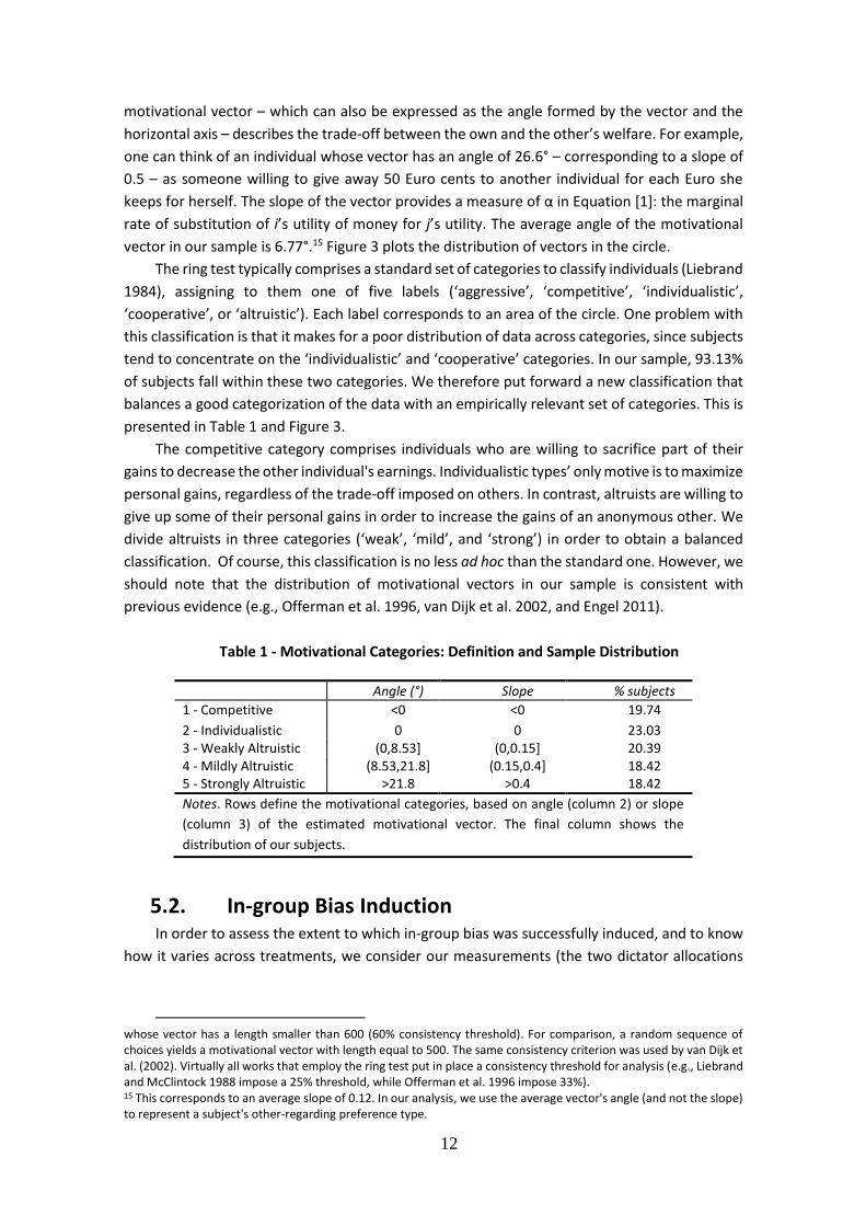
vector in our sample is 6.77°.15 Figure 3 plots the distribution of vectors in the circle.

The ring test typically comprises a standard set of categories to classify individuals (Liebrand

1984), assigning to them one of five labels (‘aggressive’, ‘competitive’, ‘individualistic’,

‘cooperative’, or ‘altruistic’). Each label corresponds to an area of the circle. One problem with

this classification is that it makes for a poor distribution of data across categories, since subjects

tend to concentrate on the ‘individualistic’ and ‘cooperative’ categories. In our sample, 93.13%

of subjects fall within these two categories. We therefore put forward a new classification that

balances a good categorization of the data with an empirically relevant set of categories. This is

presented in Table 1 and Figure 3.

The competitive category comprises individuals who are willing to sacrifice part of their

gains to decrease the other individual's earnings. Individualistic types’ only motive is to maximize

personal gains, regardless of the trade-off imposed on others. In contrast, altruists are willing to

give up some of their personal gains in order to increase the gains of an anonymous other. We

divide altruists in three categories (‘weak’, ‘mild’, and ‘strong’) in order to obtain a balanced

classification. Of course, this classification is no less ad hoc than the standard one. However, we

should note that the distribution of motivational vectors in our sample is consistent with

previous evidence (e.g., Offerman et al. 1996, van Dijk et al. 2002, and Engel 2011).

Table 1 - Motivational Categories: Definition and Sample Distribution

Angle (°) Slope % subjects

1 - Competitive <0 <0 19.74

2 - Individualistic 0 0 23.03 3 - Weakly Altruistic (0,8.53] (0,0.15] 20.39 4 - Mildly Altruistic (8.53,21.8] (0.15,0.4] 18.42 5 - Strongly Altruistic >21.8 >0.4 18.42

Notes. Rows define the motivational categories, based on angle (column 2) or slope

(column 3) of the estimated motivational vector. The final column shows the

distribution of our subjects.

5.2. In-group Bias Induction In order to assess the extent to which in-group bias was successfully induced, and to know

how it varies across treatments, we consider our measurements (the two dictator allocations

whose vector has a length smaller than 600 (60% consistency threshold). For comparison, a random sequence of choices yields a motivational vector with length equal to 500. The same consistency criterion was used by van Dijk et al. (2002). Virtually all works that employ the ring test put in place a consistency threshold for analysis (e.g., Liebrand and McClintock 1988 impose a 25% threshold, while Offerman et al. 1996 impose 33%). 15 This corresponds to an average slope of 0.12. In our analysis, we use the average vector's angle (and not the slope) to represent a subject's other-regarding preference type.

13

and the self-reported attachment to in-group and out-group in the questionnaire). Figure 4

presents results from both measures.

The percentage allocated to the in-group member achieves its highest value in High. Using

each subject’s average of the two allocation decisions as the unit of observation, we obtain

significant differences between High and the other two treatments (two-sided Mann-Whitney

test p=0.01 and p=0.03 for comparisons with Low and Control, respectively; ‘MW’ henceforth).16

High is also different from Low and Control treatments, both before (MW p=0.06 and p=0.08)

and after (MW p=0.10 and p=0.03) the participation game with marginal significance. Allocation

decisions in the Low treatment are not statistically different from those of Control (MW, p>0.75

for separate and average comparisons).

In the High treatment, a subject allocates approximately 80% of the total amount to the

member of his or her own group before the participation game; in the Low and the Control

treatments this figure is lower (approximately 72%). These numbers are in line with those

typically found in the literature (e.g., Chen and Li 2009 find values in the 65-75% range).

Allocations before and after the participation game are not statistically different, neither overall

nor for any specific treatment (MW, all p>0.59). Finally note that the results for the Low and

Control treatments provide some support for the minimal group paradigm (Tajfel 1982); subjects

give more to the in-group member than to someone from the out-group, even when no in-group

bias is induced.

Figure 3 – Distribution of subjects over motivational categories

Notes. SA/MA/WA/C stand for the categories Strong Altruist/Mild Altruist/Weak Altruist/Competitor. The Individualist category coincides with the horizontal axis.

16 Using a one-tailed t-test, a 5% significance level, and assuming: i) an expected difference of 20 percentage points

(i.e., 0.20) between High and Low, ii) a difference of 0.1 between both High and Control and Control and Low, iii) a

standard deviation of 0.2 in all treatments, the ex ante power of the statistical test is 99.9% for the High-Low

comparison, and 78.9% for the other two comparisons.

Other’s Payoff

Own Payoff

14

The results of the allocation decisions are corroborated by the second indicator of in-group

bias. In the questionnaire, subjects were asked to report their attachment to the in-group and

the out-group on a 1-to-10 scale. 17 Computing the difference between these two values yields

a measure of in-group bias on a -10-to-10 scale (see Figure 4). Average in-group bias is 3.9 in

High, 2.2 in Low, and 2.9 in Control. The difference between High and Low is statistically

significant (MW, p=0.01), while those between High and Control, and Low and Control, are not

(MW, p=0.37 and p=0.27, respectively).18

The purpose of our procedure was to create distinct levels of in-group bias between the

High and the Low treatments. In particular, we conjectured that subjects in High would show

higher levels of in-group favoritism, as the out-group has a different ‘laboratory identity’. In

contrast, the out-group in Low shares the same ‘laboratory identity’. The results presented in

Figure 4 and the corresponding statistical tests show that our procedure was successful, albeit

that the differences are relatively small. This analysis is disaggregated for the different other-

regarding preference types in Appendix D.19

As mentioned when we discussed the experimental design, for our inference to be valid

openness should neither be correlated with ring-test outcomes nor with choices in the

participation game. We find statistical evidence in favor of both requisites. Namely, only

Agreeableness seems to be significantly correlated with participation behavior, and no

personality trait seems to be significantly correlated with other-regarding preferences as

measured by the ring test.20

17 The questions are reproduced in Appendix E. 18 Using the same procedure as before to calculate power, and assuming: i) an expected difference of 2 points

between High and Low, ii) a difference of 1 point between both High and Control and Control and Low, iii) a standard

deviation of 2.5 in all treatments, the ex ante power of the statistical test is 99.7% for the High-Low comparison, and

62.4% for the other two comparisons. 19 With respect to other-regarding preferences and in-group bias, two questions can naturally be raised: what types are most likely to show a high degree of in-group favoritism, and what types are more likely to be influenced in their in-group bias by interaction in the participation game? In sum, Appendix D yields two main findings on the interaction between other-regarding preferences and in-group bias. First, on aggregate, in-group bias does not differ systematically across types. Second, except for Competitors, in-group bias is not affected by the interaction with others in the participation game. 20 See Table C 2 in the Appendix. The lack of a relationship between openness and other-regarding preferences in our data should not come as a surprise. Most of the literature finds no relationship between openness and other-regarding preferences, even though a relationship is often found for other personality traits (e.g., Ben-Ner et al. 2004, 2008, Bekkers 2006, Swope et al. 2008).

15

Figure 4 - In-group Bias Induction Across Treatments.

Notes. Bars show the fraction of the endowment allocated to the member of the in-group

(left axis). Dark gray (light gray) gives the measurement before (after) the participation

game. The difference in reported attachment to the own and other groups is given by the

connected dots (right axis). The dashed lines represent 95% confidence intervals.

5.3. Other-regarding Preferences and Participation

Behavior We now turn to our main research question, which is how participation is affected by other-

regarding preferences and in-group bias. We start by relating motivational vectors to choices in

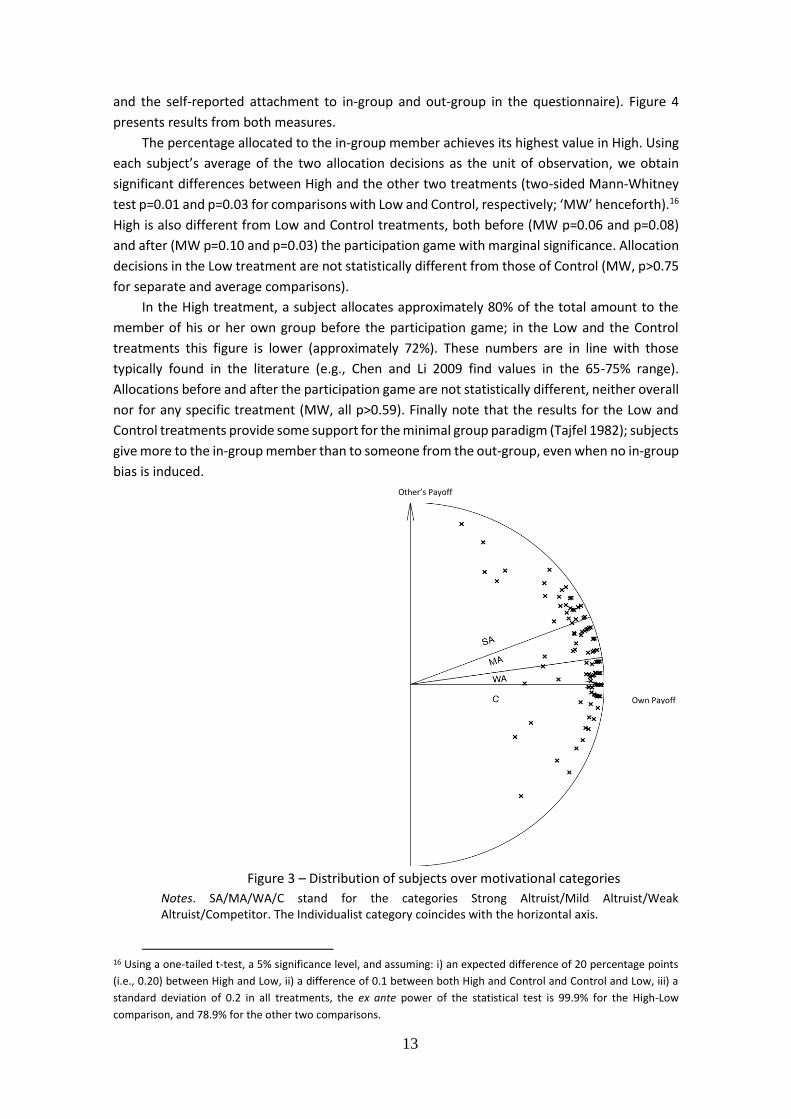
the participation game. Figure 5 presents average participation rates for each type throughout

the participation game. We observe that competitive individuals clearly participate less often

than any other type. The difference between the individual average participation of competitors

and any other category is statistically significant (MW p<0.01 for all comparisons).21 There are

no other statistical differences once we exclude competitors.

Consistent with previous evidence, there is a tendency for participation levels to decrease

as the game unfolds (e.g., Schram and Sonnemans 1996a). Regressing each type’s average

participation on a linear trend yields a negative and significant relationship for all types except

strong altruists, who exhibit a positive, albeit non-significant, increase in participation over time

(see Table C 4 in Appendix C). We conclude that strong altruists are the only type whose

cooperative behavior towards the in-group does not decrease over time.

21 Our non-parametric tests of type behavior use individual average participation over the 40 periods as the unit of observation. Non-parametric tests of aggregate behavior use the average participation of a pair of competing groups (an electorate) as the unit of observation. Using the same procedure as before for power calculations, and assuming: i) a 10% difference between average individual participation across types, ii) a 15% standard deviation within each type, and iii) an equal distribution of the sample over the 5 categories, i.e., 32 subjects of each type, results in an ex ante power of 84.61%.

16

Figure 5 - Evolution of Participation and Motivational Categories.

Notes. Average participation rates of participants of a given motivational category.

In order to see in more detail how participation depends on other-regarding preferences,

Figure 6 shows a scatter plot of individual participation rates for each type, as well as a fitted

least squares trend. We observe that the relationship between the individual participation rate

(i.e., the fraction of the 40 periods that a subject chose to participate) and other-regarding

concerns (measured by the angle of the motivational vector) is positive for most categories (by

definition, there is no such relationship for the Individualistic category). A regression of

individual average participation on the degree of other-regarding preferences produces a

positive coefficient for each category, even though statistical significance is only achieved when

considering the full sample and (marginally so) for the group of strong altruists (see Table 2). As

conjectured, individual average participation is increasing in a subject's other-regarding

preferences.

All in all, our analysis shows that there is a positive relationship between other-regarding

preferences and participation behavior. The effect is statistically strong at the aggregate level

and appears to be present for each of the categories we distinguished. A pronounced difference

is observed for the category of competitors, who significantly abstain more than other types.

This evidence lends support to Hypothesis 1.

17

Table 2 - Participation and Other-Regarding Preferences

All Categories Competitor Weak A. Mild A. Strong A.

Motivational Vector (°) 0.024*** 0.012 0.176 0.002 0.038*

(2.92) (0.60) (1.40) (0.03) (1.70)

Constant 1.645*** 1.114*** 1.386* 2.028* 0.175

(8.97) (3.02) (1.83) (1.65) (0.21)

Notes: Panel regression (logit with random effects at the individual level); N=152. Dependent variable:

average individual participation in the 40 periods of the participation game. A trend and a squared trend

terms are included as controls, but not reported. Absolute z-scores in parentheses. *** (**, *) indicates

significance at the 1% (5%, 10%) level.

Figure 6 - Individual Participation Rates and Other-Regarding Preferences. Notes. The plotted line is a linear least squares trend fitted to the entire sample.

5.4. In-group bias and Participation Behavior Our second and third hypotheses concern the relationship between in-group bias and

participation behavior. As formulated in Hypothesis 2a, we expect electorates where in-group

bias is stronger to exhibit higher levels of aggregate participation. At the individual level, Hypo-

thesis 2b predicts that subjects with higher in-group bias participate more often.

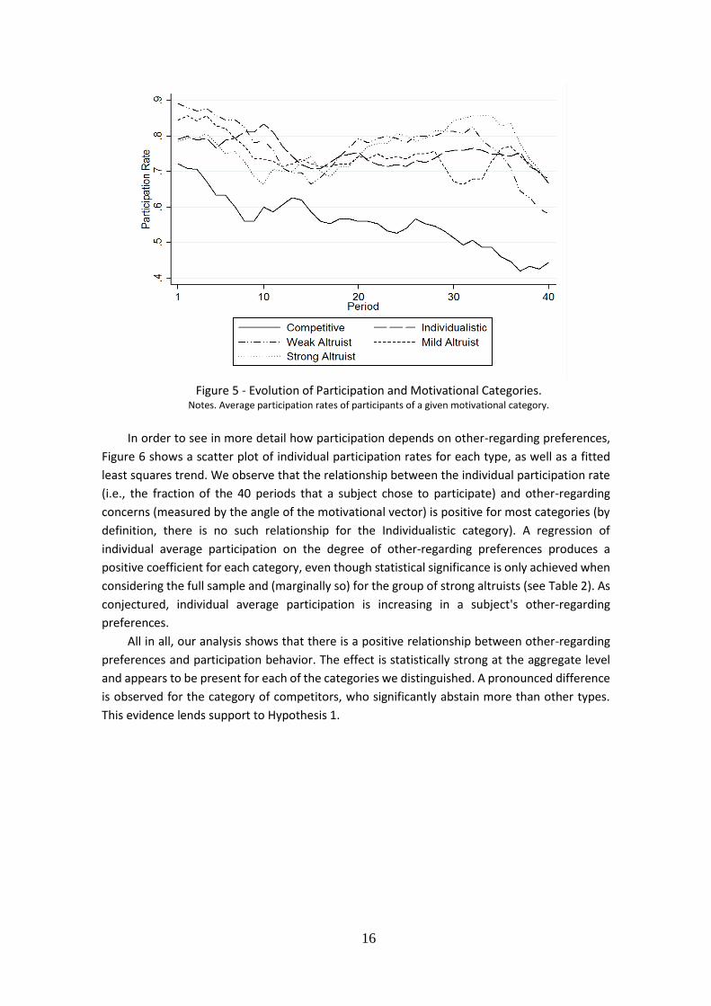
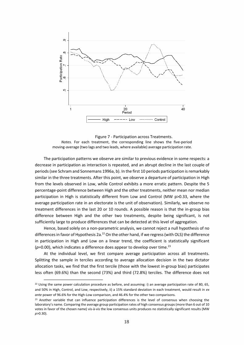
Figure 7 shows aggregate participation levels for each of the three treatments across the

40 periods of the participation game. Aggregate participation rates are highest in the treatment

High (74.3%), followed by Low (69.3%) and Control (69.2%). Participation variance is lowest in

High, followed by Low and Control (standard deviations equal to 4.3%, 7.1% and 10.9%,

respectively).

18

Figure 7 - Participation across Treatments. Notes. For each treatment, the corresponding line shows the five-period

moving-average (two lags and two leads, where available) average participation rate.

The participation patterns we observe are similar to previous evidence in some respects: a

decrease in participation as interaction is repeated, and an abrupt decline in the last couple of

periods (see Schram and Sonnemans 1996a, b). In the first 10 periods participation is remarkably

similar in the three treatments. After this point, we observe a departure of participation in High

from the levels observed in Low, while Control exhibits a more erratic pattern. Despite the 5

percentage-point difference between High and the other treatments, neither mean nor median

participation in High is statistically different from Low and Control (MW p>0.33, where the

average participation rate in an electorate is the unit of observation). Similarly, we observe no

treatment differences in the last 20 or 10 rounds. A possible reason is that the in-group bias

difference between High and the other two treatments, despite being significant, is not

sufficiently large to produce differences that can be detected at this level of aggregation.

Hence, based solely on a non-parametric analysis, we cannot reject a null hypothesis of no

differences in favor of Hypothesis 2a.22 On the other hand, if we regress (with OLS) the difference

in participation in High and Low on a linear trend, the coefficient is statistically significant

(p=0.00), which indicates a difference does appear to develop over time.23

At the individual level, we first compare average participation across all treatments.

Splitting the sample in terciles according to average allocation decision in the two dictator

allocation tasks, we find that the first tercile (those with the lowest in-group bias) participates

less often (69.6%) than the second (73%) and third (72.8%) terciles. The difference does not

22 Using the same power calculation procedure as before, and assuming: i) an average participation rate of 80, 65,

and 50% in High, Control, and Low, respectively, ii) a 15% standard deviation in each treatment, would result in ex

ante power of 96.6% for the High-Low comparison, and 46.4% for the other two comparisons. 23 Another variable that can influence participation differences is the level of consensus when choosing the laboratory’s name. Comparing the average group participation rates of high consensus groups (more than 6 out of 10 votes in favor of the chosen name) vis-à-vis the low consensus units produces no statistically significant results (MW p>0.30).

19

reach statistical significance when we use individual average participation as the unit of

observation, however (MW p>0.21). At this level of aggregation, we find no support for

Hypothesis 2b. Below, we will see that more support for the alternative Hypothesis 2b is

obtained when employing a multivariate analysis framework.

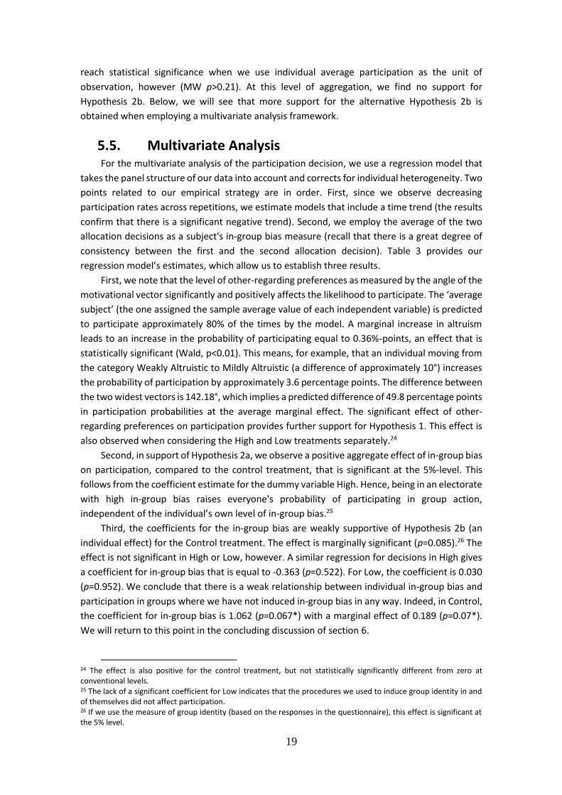
5.5. Multivariate Analysis For the multivariate analysis of the participation decision, we use a regression model that

takes the panel structure of our data into account and corrects for individual heterogeneity. Two

points related to our empirical strategy are in order. First, since we observe decreasing

participation rates across repetitions, we estimate models that include a time trend (the results

confirm that there is a significant negative trend). Second, we employ the average of the two

allocation decisions as a subject's in-group bias measure (recall that there is a great degree of

consistency between the first and the second allocation decision). Table 3 provides our

regression model’s estimates, which allow us to establish three results.

First, we note that the level of other-regarding preferences as measured by the angle of the

motivational vector significantly and positively affects the likelihood to participate. The ‘average

subject’ (the one assigned the sample average value of each independent variable) is predicted

to participate approximately 80% of the times by the model. A marginal increase in altruism

leads to an increase in the probability of participating equal to 0.36%-points, an effect that is

statistically significant (Wald, p<0.01). This means, for example, that an individual moving from

the category Weakly Altruistic to Mildly Altruistic (a difference of approximately 10°) increases

the probability of participation by approximately 3.6 percentage points. The difference between

the two widest vectors is 142.18°, which implies a predicted difference of 49.8 percentage points

in participation probabilities at the average marginal effect. The significant effect of other-

regarding preferences on participation provides further support for Hypothesis 1. This effect is

also observed when considering the High and Low treatments separately.24

Second, in support of Hypothesis 2a, we observe a positive aggregate effect of in-group bias

on participation, compared to the control treatment, that is significant at the 5%-level. This

follows from the coefficient estimate for the dummy variable High. Hence, being in an electorate

with high in-group bias raises everyone's probability of participating in group action,

independent of the individual’s own level of in-group bias.25

Third, the coefficients for the in-group bias are weakly supportive of Hypothesis 2b (an

individual effect) for the Control treatment. The effect is marginally significant (p=0.085).26 The

effect is not significant in High or Low, however. A similar regression for decisions in High gives

a coefficient for in-group bias that is equal to -0.363 (p=0.522). For Low, the coefficient is 0.030

(p=0.952). We conclude that there is a weak relationship between individual in-group bias and

participation in groups where we have not induced in-group bias in any way. Indeed, in Control,

the coefficient for in-group bias is 1.062 (p=0.067*) with a marginal effect of 0.189 (p=0.07*).

We will return to this point in the concluding discussion of section 6.

24 The effect is also positive for the control treatment, but not statistically significantly different from zero at conventional levels. 25 The lack of a significant coefficient for Low indicates that the procedures we used to induce group identity in and of themselves did not affect participation. 26 If we use the measure of group identity (based on the responses in the questionnaire), this effect is significant at the 5% level.

20

Table 3 – Panel Regression Model

Coefficient Marginal effect

Motivational Vector Angle

0.022*** 0.004***

(2.74) (2.69)

In-group bias 0.980* 0.158*

(1.72) (1.71)

High 1.096** 0.162**

(2.07) (2.23)

Low 0.397 0.062

(0.89) (0.92)

Trend -0.032*** -0.005***

(2.66) (2.61)

In-group bias*High -1.336* -0.215*

(1.72) (1.72)

In-group bias*Low -0.961 -0.155

(1.31) (1.31)

Constant 1.083*** ---

(2.99) ---

Notes Cells present the panel logit estimation (with random effects at the individual level) coefficients (column 2) and marginal effects (column 3); N=152. Dependent variable: individual participation in each of the 40 periods. High and Low are dummy variables representing these treatments. In-group bias is measured as the average of the two dictator allocation decisions, re-scaled to the interval [-1,1]. Absolute z-scores in parentheses. * (**, ***) indicates significance at the 10% (5%, 1%) level. Marginal effects are computed for the mean sample values of our variables.

5.6. Conclusions with respect to our Hypotheses To sum up, we find robust evidence in favor of a positive relationship between individual

participation and other-regarding preferences (Hypothesis 1). The data depicted in Figure 6 and

the regression analysis of Table 2, together with the significant coefficient obtained in the panel

models, provide ample evidence in this respect. Regarding the conjecture that participation

should be higher in the High treatment (Hypothesis 2a), we find confirming evidence when we

use the panel regression framework, in spite of the inconclusive evidence reported in section

5.4. We also show that, whenever in-group bias is not manipulated (the Control treatment),

there is tentative evidence that subjects who show a higher degree of in-group bias tend to

participate more (Hypothesis 2b).

6. Conclusion This paper is an attempt to contribute evidence from a controlled environment to the

stream of literature that tries to evaluate political participation in light of other-regarding

concerns and group-directed duties. In particular, we have used an experimental framework to

address the influence of other-regarding motivations and in-group bias on political participation

21

decisions. Our work follows in the footsteps of the emerging rational choice literature that puts

forward a ‘group-based model of turnout’, as put forward by Feddersen (2004).

The empirical literature in political science and psychology has shown that group identity

sentiments that result in in-group bias help explain patterns of individual political participation

among several groups in society (e.g., Leighley and Vedlitz 1999 and Stokes 2003). However,

establishing a causal link in the field poses considerable challenges, mostly because of the co-

evolution of group identity, social connectedness, and group mobilization processes.

In this paper we report evidence from an environment where in-group bias is varied in a

controlled fashion and in which we can observe the behavior of groups that subsequently

compete for benefits. Victory depends on the sum of the individual efforts by the individuals in

a group. Despite the extensive literature that analyzes the relationship between in-group bias

and individual and group behavior in the laboratory, we believe to be the first, together with

Cason et al. (2016), to do so in the context of inter-group competition.

Our main conclusions are that individual participation is increasing in other-regarding

concerns and in-group bias, as conjectured. We also found support for an impact of in-group

bias on aggregate participation levels (but only in a multivariate analysis that corrects for the

influence of confounding factors). This latter result implies that the higher participation levels

observed in field studies for environments where group identity is high (e.g., contexts with

pronounced ethnic divisions and high political participation) might be due to this heightened

sense of group identity. Whether group mobilization adds something to this effect is a question

for further research.

Finally, there is a modest correlation between individual-level sense of in-group bias and

participation in our Control treatment, i.e., when we did not induce any in-group bias. In this

case, people with a large bias towards the in-group tend to participate more in political action.

When we induce a high sense of in-group bias at the electorate level, individual differences still

exist, but no longer matter for the participation decision. Similarly, when our procedures induce

bias towards both the in-group and the out-group, differences still exist (at a lower level), but

do not matter for participation. In other words, individual differences within a group matter only

when people experience moderate differences between the groups.

These results can be interpreted in light of Fowler (2006), who has shown that other-

regarding subjects only participate more often in politics if they are strong party identifiers. We

have shown that a positive relationship between other-regarding preferences and participation

exists even if we control for in-group bias. In the world outside the laboratory, it seems natural

that more generous party identifiers participate more, as they believe that their supported party

will improve the well-being of their fellow citizens. We show that, more generally, individuals

with pro-social motives are more likely to bear the costs of participation for the group’s benefit.

Our results suggest that, in principle, all individuals with other-regarding concerns should be

willing to participate, provided there exist platforms that advance their group’s interests.

All in all, we conclude that other-regarding individuals participate more. Moreover, a

common sense of identification with the group yields higher aggregate levels of political

participation. As described above, the effect of in-group bias is more complex at the individual

level and depends on experienced differences between groups. Each of these results may serve

as input in a canonical model as envisaged by Feddersen (2004).

22

References Aldrich, J. A. (1997). “When is it rational to vote?”, in (D. Mueller, ed.), Perspectives on

Public Choice, a Handbook, Cambridge: Cambridge University Press, 379-390.

Bekkers, R. (2006). “Traditional and health-related philanthropy: The role of resources and

personality.” Social Psychology Quarterly, 69(4), 349-366.

Ben-Ner, A., Kong, F. & Putterman, L. (2004). “Share and share alike? Gender-pairing,

personality, and cognitive ability as determinants of giving.” Journal of Economic Psychology,

25(5), 581-589.

Ben-Ner, A., Kramer, A. & Levy, O. (2008). “Economic and hypothetical dictator game

experiments: Incentive effects at the individual level.” The Journal of Socio-Economics, 37(5),

1775-1784.

Blais, A. (2000). To vote or not to vote?: The merits and limits of rational choice theory.

University of Pittsburgh Press.

Bornstein, G. (1992). “The Free-Rider Problem in Intergroup Conflicts Over Step-Level and

Continuous Public Goods.” Journal of Personality and Social Psychology 62 (April), 597-606.

Bornstein, G., Rapoport, A., Kerpel, L. & Katz, T. (1989). “Within- and Between-Group

Communication in Intergroup Competition for Public Goods.” Journal of Experimental Social

Psychology 25, 422-436.

Bornstein, G., Gneezy, U. & Nagel, R. (2002). “The effect of intergroup competition on

group coordination: An experimental study.” Games and Economic Behavior, 41(1), 1-25.

Brewer, M. (2007). “The Social Psychology on Intergroup Relations: Social Categorization,

Ingroup Bias, and Outgroup Prejudice.” in Social Psychology: Handbook of Basic Principles,

Kruglanski, A., and E. Higgins (eds.), The Guilford Press, New York.

Cason, T. N., Laub, S. H. P. & Muic, V. L. (2016). “Prior Interaction, Identity, and

Cooperation in the Inter-Group Prisoner’s Dilemma.”, Working Paper.

Carney, D. R., Jost, J. T., Gosling, S. D. & Potter, J. (2008). “The secret lives of liberals and

conservatives: Personality profiles, interaction styles, and the things they leave behind.” Political

Psychology, 29(6), 807-840.

Charness, G., Rigotti, L. & Rustichini, A. (2007). “Individual Behavior and Group

Membership.” American Economic Review, 97(4), 1340-1352.

Chen, Y. & Li, S. (2009). “Group Identity and Social Preferences.” American Economic

Review, 99(1), 431-457.

Dawes, C., Loewen, P. & Fowler, J. (2011). “Social Preferences and Political Participation.”

The Journal of Politics 73(3), 845-856.

Dhillon, A. & Peralta, S. (2002). “Economic theories of voter turnout”. The Economic

Journal, 112(480), 332-352.

Diehl, M. (1990). “The minimal group paradigm: Theoretical explanations and empirical

findings.” European Review of Social Psychology 1(1), 263-292.

Eckel, C. & Grossman, P. (2005). “Managing diversity by creating team identity.” Journal of

Economic Behavior & Organization 58, 371-392.

Edlin, A., Gelman, A. & Kaplan, N. (2007). “Voting as a Rational Choice: Why and How

People Vote to Improve the Well-Being of Others.” Rationality and Society 19(3), 293-314.

Ellemers, N. (2012). “The group self.” Science, 336(6083), 848-852.

Engel, C. (2011). “Dictator games: A meta study.” Experimental Economics, 14(4), 583-610.

23

Evren, Ö. (2012). “Altruism and voting: A large-turnout result that does not rely on civic

duty or cooperative behavior.” Journal of Economic Theory 147, 6, 2124-2157.

Feddersen, T. (2004). “Rational Choice Theory and the Paradox of Not Voting.” The Journal

of Economic Perspectives 18(1), 99-112.

Feddersen, T., Gailmard, S. & Sandroni, A. (2009). “Moral bias in large elections: Theory

and experimental evidence.” American Political Science Review 103, 175-192.

Fehr, E., & Schmidt, K. M. (1999). “A theory of fairness, competition, and cooperation.”

The Quarterly Journal of Economics 114(3), 817-868.

Fischbacher, U. (2007) “z-Tree: Zurich toolbox for ready-made economic experiments.”

Experimental Economics 10(2), 171-178.

Fowler, J. (2006). “Altruism and Turnout.” The Journal of Politics 68(3), 674-83.

Fowler, J. & Kam, C. (2007). “Beyond the Self: Social Identity, Altruism, and Political

Participation.” The Journal of Politics 69(3), 813-827.

Gerber, A. S., Huber, G. A., Doherty, D., Dowling, C. M., Raso, C. & Ha, S. E. (2011).

“Personality traits and participation in political processes.” Journal of Politics, 73(3), 692-706.

Goeree, J. K. & Holt, C. A. (2005). An explanation of anomalous behavior in models of

political participation. American Political Science Review 99(2), 201-213.

Goren, H. & Bornstein, G. (2000). “The Effects of Intragroup Communication on Intergroup

Cooperation in the Repeated Intergroup Prisoner's Dilemma (IPD) Game.” Journal of Conflict

Resolution 44(5), 700-719.

Grosser, J. & Schram, A. (2006). “Neighborhood information exchange and voter

participation: an experimental study.” American Political Science Review, 100(2), 235-248.

Hogg, A. & Abrams, D. (1998). Social Identifications: A Social Psychology of Intergroup

Relations and Group Processes, Routledge, London.

Jankowski, R. (2002). “Buying a Lottery Ticket to Help the Poor: Altruism, Civic Duty, and

Self-interest in the Decision to Vote.” Rationality and Society 14, 55-77.

Jankowski, R. (2007). “Altruism and the Decision to Vote: Explaining and Testing High Voter

Turnout.” Rationality and Society 19, 5-34.

John, O., Naumann, L. & Soto, C. (2008). “Paradigm Shift to the Integrative Big-Five Trait

Taxonomy: History, Measurement, and Conceptual Issues.” In O. P. John, R. W. Robins & L. A.

Pervin (Eds.), Handbook of personality: Theory and research, 114-158. New York, NY: Guilford

Press.

Jost, J. T., Glaser, J., Kruglanski, A. W. & Sulloway, F. J. (2003). “Political conservatism as

motivated social cognition.” Psychological bulletin, 129(3), 339.

Jost, J. T. (2006). “The end of the end of ideology.” American Psychologist, 61(7), 651.

Knack, S. (1992). “Social Altruism and Voter Turnout: Evidence from the 1991 NES Pilot

Study.” 1991 NES Pilot Study Reports.

Leighley, J. & Vedlitz, A. (1999). “Race, Ethnicity, and Political Participation: Competing

Models and Contrasting Explanations.” The Journal of Politics 61(4), 1092-1114.

Liebrand, W. (1984). “The effect of social motives, communication and group size on

behavior in an n-person multi stage mixed motive game.” European Journal of Social Psychology

14, 239-264.

Liebrand, W. B. & McClintock, C. G. (1988). The ring measure of social values: A

computerized procedure for assessing individual differences in information processing and

social value orientation. European Journal of Personality, 2(3), 217-230.

24

Lijphart, A. (1997). “Unequal Participation: Democracy’s Unresolved Dilemma.” American

Political Science Review 91 (March), 1-14.

McKelvey, R. D. & Palfrey, T. R. (1995): “Quantal response equilibria for normal form

games.” Games and economic behavior 10(1), 6-38.

Mondak, J. J., Hibbing, M. V., Canache, D., Seligson, M. A. & Anderson, M. R. (2010).

“Personality and civic engagement: An integrative framework for the study of trait effects on

political behavior.” American Political Science Review 104(1), 85-110.

Morton, R. B. (1991). “Groups in rational turnout models.” American Journal of Political

Science, 35(3), 758-776.

Mutz, D. (2002). “The Consequences of Cross-Cutting Networks for Political Participation.”

American Journal of Political Science 46 (October), 838--55.

Offerman, T., Sonnemans, J. & Schram, A. (1996). “Value orientations, expectations and

voluntary contributions in public goods.” Economic Journal 106, 817--845.

Palfrey, T. R. (2009). “Laboratory Experiments in Political Economy.” Annual Review of Political Science 12, 379-388.

Palfrey, T. R. & Rosenthal, H. (1983). “A Strategic Calculus of Voting.” Public Choice 41(1),

7-53.

Rabbie, J. M. & Wilkens, G. (1971). “Intergroup competition and its effect on intragroup

and intergroup relations.” European Journal of Social Psychology, 1(2), 215-234.

Riechmann, T. & Weimann, J. (2008). “Competition as a coordination device: Experimental

evidence from a minimum effort coordination game.” European Journal of Political Economy,

24(2), 437-454.

Schram, A. & Sonnemans, J. (1996a). “Voter Turnout and the Role of Groups: Participation Game Experiments.” International Journal of Game Theory 25, 385-406.

Schram, A. & Sonnemans, J. (1996b). “Why People Vote: Experimental Evidence.” Journal of Economic Psychology 17 (4), 417-442.

Schram, A. & van Winden, F. (1991). “Why People Vote. Free Riding and the Production

and Consumption of Social Pressure.” Journal of Economic Psychology 12(4), 575-620.

Sen, A. K. (1977). “Rationality and morality: A reply.” Erkenntnis, 11(1), 225-232.

Shachar, R. & Nalebuff, B. (1999). “Follow the leader: Theory and evidence on political

participation.” American Economic Review, 89(3), 525-547.

Simon, B., Loewy, M., Stürmer, S., Weber, U., Freytag, P., Habig, C., Kampmeier, C. &

Spahlinger, P. (1998). “Collective identification and social movement participation.” Journal of

personality and social psychology, 74(3), 646-658.

Stokes, A. K. (2003). “Latino group consciousness and political participation.” American

Politics Research, 31(4), 361-378.

Stürmer, S. & Simon, B. (2004). “Collective action: Towards a dual-pathway model.”

European Review of Social Psychology, 15(1), 59-99.

Swope, K. J., Cadigan, J., Schmitt, P. M. & Shupp, R. (2008). “Personality preferences in

laboratory economics experiments.” The Journal of Socio-Economics, 37(3), 998-1009.

Tajfel, H. (1982). “Social Psychology of Intergroup Relations.” Annual Review of Psychology

33, 1-39.

van Dijk, F., Sonnemans, J. & van Winden, F. (2002). “Social Ties in a Public Good

Experiment.” Journal of Public Economics 85 (2), 275-299.

Verba, S. & Nie, N. (1972). Participation in America: Political Democracy and Social Equality.

New York: Harper and Row.

25

Appendix

A. Equilibria of the Participation Game In this Appendix, we formally derive the equilibria of the participation game, which allows

us to obtain comparative static results on the hypotheses we want to test.27 Define the set of

players as 𝐼 = [1, . . . , 𝑀,𝑀 + 1, . . . , 𝑀 + 𝑁], where 𝑀 and 𝑁 are the number of players in groups

1 and 2, respectively. We denote the in-group and the out-group of player 𝑖 by 𝐺𝑖 and 𝐺−𝑖,

respectively. We consider the case where 𝑀 = 𝑁 and both are odd. The action space of a player

has two elements: participation and non-participation. A (mixed) strategy is simply a probability

of participation, which is denoted by 𝑝.

We posit individual preferences that accommodate general altruism towards others, as well

as discrimination between in-group and out-group members:

𝑈𝑖 = 𝑈𝑖(𝑢𝑖(𝑥𝑖); 𝑈𝑗 , 𝑗 ∊ 𝐺𝑖\𝑖; 𝑈ℎ , ℎ ∊ 𝐺−𝑖; 𝛼𝑖, 𝛽𝑖, 𝛾𝑖) [1A]

In Equation [1A], 𝑈𝑖 denotes i’s utility, 𝑥𝑖 gives her monetary earnings, and 𝑢𝑖(𝑥𝑖) describes

her utility of wealth. 𝛼𝑖 is a parameter describing the weight 𝑖 attributes to the others’ utility,

relative to her own, 𝛽𝑖 is the weight she attributes to the utility of other members in her own

group, and 𝛾𝑖 is the weight she attributes to the utility of members in the other group.

To derive comparative statics for the participation game, we make the following three

assumptions:

1. If members of the own group receive higher utility from an outcome than members

of the other group do, then more in-group bias leads to higher utility:

𝑈𝑗,𝑗∊𝐺𝑖\𝑖 > 𝑈ℎ,ℎ∊𝐺−𝑖 ⇒𝜕𝑈𝑖

𝜕𝛽𝑖> 0 [2A]

2. If members of the own group receive lower utility from an outcome than members

of the other group, then more in-group bias leads to lower utility:

𝑈𝑗,𝑗∊𝐺𝑖\𝑖 < 𝑈ℎ,ℎ∊𝐺−𝑖 ⇒𝜕𝑈𝑖

𝜕𝛽𝑖< 0 [3A]

3. The utility derived from winning the participation game (and, as a consequence, 𝑗 ∊

𝐺𝑖\𝑖 also winning and ℎ ∊ 𝐺−𝑖 losing the participation game) is larger than the utility

derived from losing the participation game (and, as a consequence, 𝑗 ∊ 𝐺𝑖\𝑖 also losing

and ℎ ∊ 𝐺−𝑖 winning the participation game):

𝑈𝑤 ≡ 𝑈𝑖(𝑥𝑖 = 𝐵𝑤 , 𝑥𝑗,𝑗∊𝐺𝑖\𝑖 = 𝐵𝑤 , 𝑥ℎ,ℎ∊𝐺−𝑖 = 𝐵𝑙)

> 𝑈𝑙 ≡ 𝑈𝑖(𝑥𝑖 = 𝐵𝑙 , 𝑥𝑗,𝑗∊𝐺𝑖\𝑖 = 𝐵𝑙 , 𝑥ℎ,ℎ∊𝐺−𝑖 = 𝐵𝑤) [4A]

27 We derive stage-game equilibria for the game our subjects play for forty rounds in fixed electorates. Due to a

multiplicity of equilibria in the one-shot game (recall that we follow the literature in considering only quasi-symmetric

equilibria) there is a plethora of equilibria in the repeated game. A repetition of the stage-game equilibrium that we

derive is one of these. Note that we only use the theory as a benchmark with which we can derive comparative statics.

26

where 𝑈𝑖𝑤 (𝑈𝑖

𝑙) is the utility in case of victory (defeat). Note that [4A] implies an intuitive

restriction on the parameters 𝛼𝑖 and 𝛽𝑖, i.e., they are such that any individual prefers the own

team winning the participation game to the other team winning.

Equations [2A]-[4A] yield:

𝜕𝑈𝑤

𝜕𝛽> 0,

𝜕𝑈𝑙

𝜕𝛽< 0 ⇒

𝜕(𝑈𝑤 − 𝑈𝑙)

𝜕𝛽> 0 [5A]

In words, [5A] states that an increase in an individual’s in-group bias will lead to a higher

marginal benefit of her group winning the participation game.

Next, we need to determine how this increased marginal benefit affects the choice to

participate. Ceteris paribus, this will yield a higher participation probability, simply because the

benefits increase while the costs remain unchanged. This is not necessarily true in an equilibrium

analysis, however, because other voters may respond to variations in an individual’s incentives.

We therefore proceed with equilibrium analysis. We assume complete information throughout:

in addition to the rules of the game, monetary payoffs and group size, we assume that players

know the utility functions of all other players. This simplification does not hinder the derivation

of broad comparative statics and keeps the analysis tractable. The alternative would be to adopt

incomplete information (i.e., players do not know the other players’ preference parameters),

which would require further ad hoc assumptions on beliefs.

We use a utility function of the type defined in [1A]. These individual preferences

accommodate general altruism towards others, as well as discrimination between in-group and

out-group members (see section 2 of the main text for an explanation of the notation):

𝑈𝑖 = 𝑢𝑖 + 𝛼𝑖 (𝛽𝑖 ∑ 𝑈𝑗 +

𝑗∊𝐺𝑖\𝑖

𝛾𝑖 ∑ 𝑈ℎ

ℎ∊𝐺−𝑖

) [6A]

The utility payoff depends on whether a player’s group wins or loses the game: define 𝛤 =

𝑤, 𝑙 as these two events. Given our preference structure, the payoffs of the game are

interdependent across players. Assuming that 𝑖 is in the winning group, [6A] can be rewritten by

substituting 𝑢𝑖 for 𝐵𝑤 and plugging in 𝐵𝑤 and 𝐵𝑙 in the utilities of the other players. The utility

if 𝑖 loses, 𝑈𝑖𝑙, can be obtained in a similar fashion. For given preferences and for each case

(winning or losing), this yields a system of 𝑀 + 𝑁 equations (the individual utilities) in 𝑀 + 𝑁

variables (the utility payoffs):

[𝐼 − Ω]𝑢(𝛤) = 𝑏(𝛤)

⇒ 𝑢(𝛤) = [𝐼 − Ω]−1𝑏(𝛤) [7A]

where 𝐼((𝑀+𝑁)×(𝑀+𝑁)) is the identity matrix,

Ω((𝑀+𝑁)×(𝑀+𝑁)) =

[

0 𝛼1𝛽1 … 𝛼1𝛽1 𝛼1𝛾1 … 𝛼1𝛾1

𝛼2𝛽2 ⋱ 𝛼2𝛾2

⋮ ⋮𝛼𝑀𝛽𝑀 𝛼𝑀𝛾𝑀

𝛼𝑀+1𝛾𝑀+1 𝛼𝑀+1𝛽𝑀+1

⋮ ⋱ ⋮𝛼𝑀+𝑁𝛾𝑀+𝑁 … 𝛼𝑀+𝑁𝛾𝑀+𝑁 𝛼𝑀+𝑁𝛽𝑀+𝑁 … 0 ]

,

𝑢(𝑤) = (𝑈1𝑤 , … , 𝑈𝑀

𝑤, 𝑈𝑁𝑙 , … , 𝑈𝑀+𝑁

𝑙 )′, and 𝑏(𝑤) = (𝐵𝑤 , … , 𝐵𝑤 , 𝐵𝑙 , … , 𝐵𝑙)′ (with the case of

𝛤 = 𝑙 defined accordingly). The solution to [7A] allows us to calculate the utility of a winning

and losing player for any combination of 𝐵𝑤 , 𝐵𝑙 , 𝑐, and other-regarding and in-group bias

parameters (Ω).

27

Following Palfrey and Rosenthal (1983), it can be shown that for the case with equal group

sizes there exists a unique Nash equilibrium in pure strategies with full participation (for 𝑐 <

(𝑈𝑤 − 𝑈𝑙)/2). In addition, a plethora of mixed-strategy Nash equilibria exist. To refine this set,

and for reasons discussed in section 3 of the main text, the analysis of participation games has

often resorted to the quantal response equilibrium concept (QRE; McKelvey and Palfrey 1995).

Adding a stochastic component to decision rules [2] and [3] in the main text, (𝜇𝜀𝑖, 𝑖 =

𝑃,𝑁𝑃, respectively) implies that a player prefers participation to non-participation if:

[Pr[𝑚 = 𝑛] + Pr[𝑚 = 𝑛 − 1]](𝑈𝑖

𝑤 − 𝑈𝑖𝑙)

2− 𝑐 > 𝜇(𝜀𝑃 − 𝜀𝑁𝑃) [8A]

where 𝜇 is a parameter that governs the extent of bounded rationality (noise) in players’

decisions, and the 𝜀𝑖 represent i.i.d. realizations of a random variable. Following much of the

literature, we assume that the difference of the errors in [8A] follows a logistic distribution. This

implies the following equilibrium condition for each player (see Goeree and Holt 2005 for

details):

𝑝𝑖 =1

1 + 𝑒𝑥𝑝

[ 𝑐 − [(Pr[𝑚 = 𝑛] + Pr[𝑚 = 𝑛 − 1])

(𝑈𝑖𝑤 − 𝑈𝑖

𝑙)2 ]

𝜇

]

, 𝑖 = 1,… ,10

[9A]

The 𝜇 parameter is typically estimated from experimental data. Goeree and Holt (2005)

show that a value of 𝜇=0.8 accommodates the data of Schram and Sonnemans (1996a), in which

participation fluctuates in the 30-50% range. Since we observe higher participation levels, our

data would possibly imply a slightly higher value of 𝜇. For our purposes the precise value of this

parameter is not particularly relevant as only point predictions, and not comparative statics, will

depend on it. For this reason, we use 𝜇=0.8, for the numerical QRE results that follow.

In-group Bias and Aggregate Participation To start, we consider totally quasi-symmetric equilibria (Palfrey and Rosental 1983) where

all voters in group 1 vote with the same probability pG1 and all voters in group 2 vote with the

same probability pG2. For participation games where both groups have an equal size the

probability terms are then defined as (for a player in group 1):

Pr[𝑚 = 𝑛] = ∑ (𝑀 − 1

𝑘)

𝑀−1

𝑘=0

(𝑁𝑘) (𝑝𝐺1)

𝑘(1 − 𝑝𝐺1)𝑀−1−𝑘(𝑝𝐺2)

𝑘(1 − 𝑝𝐺2)𝑁−𝑘 [10A]

Pr[𝑚 = 𝑛 − 1] = ∑ (𝑀 − 1

𝑘)

𝑀−1

𝑘=0

(𝑁

𝑘 + 1) (𝑝𝐺1)

𝑘(1 − 𝑝𝐺1)𝑀−1−𝑘(𝑝𝐺2)

𝑘+1(1

− 𝑝𝐺2)𝑁−𝑘−1

[11A]

The assumption that in equilibrium every player in the same group participates with the

same probability can be intuitively justified by the assumption that players are homogenous in

their other-regarding preferences. For our analysis, we further assume here that players in both

groups have the same parameters (and therefore, pG1 = pG2 = p), which means that we will

investigate how equilibria change when we vary the in-group bias parameters for all players.

Our strategy is to numerically determine the equilibrium p for distinct parameters and to derive

comparative static predictions from comparing these equilibria.

28

We first determine the effect of in-group bias for this homogenous case. With respect to

the preferences put forward in [6A] (with αi = α, βi = βi, γi = γ, i) we implement five

parameterizations that use 𝛼 = 0.12 (the average slope of the motivational vector in our data)

but have different in-group bias ratios β/γ = 0, 1/3, 1, 3,∞. For each parameter

configuration, we solve [7A] and substitute the result and the above probabilities in [9A] and

solve for p. This yields the QRE 𝑝 = 0.26, 0.28, 0.32, 0.48, 0.58, respectively These are also

the predicted levels of aggregate participation. We conclude that for the homogenous case, and

the moderate level of altruistic concerns found in our data (𝛼 = 0.12), equilibrium (aggregate)

participation is increasing in in-group bias.

The same is true for the parameters obtained via a standard maximum likelihood procedure

performed on our experimental data from the participation game. The likelihood function is the

product of the likelihood contributions of each single individual decision in the participation

game. Holding the QRE error parameter constant at 0.8, we computed the (log-)likelihood for

several combinations of parameter values. We implemented a combination of values of α

between 0.1 and 2, in steps of 0.1 (20 values), and of values of β/γ between 2/3 and 8/3, in

steps of 0.1(20 values). We imposed the restriction that 𝛽𝑖+𝛾𝑖=1, as mentioned above. Using a

grid search, we conclude that the (log-)likelihood is maximized for α=0.5 and β/γ=2.067 (Log-

likelihood=-3618.56). Note that the magnitude of 𝛼 depends on the normalization chosen for

𝛽𝑖+𝛾𝑖.

Altruism, In-group Bias, and Individual Participation Next, we drop the assumed homogeneity and allow for different mixed strategies for each

player. This enables an investigation of the comparative statics at the individual level. The

probability terms become, for each player 𝑖:

Pr[𝑚 = 𝑛] = ∑∏𝑝ℎ

𝐴𝑗𝑘

ℎ≠𝑖

126

𝑗=1

(1 − 𝑝ℎ)(1−𝐴𝑗𝑘), 𝑘 = ℎ, 𝑖𝑓 ℎ < 𝑖ℎ − 1, 𝑒𝑙𝑠𝑒

[12A]

Pr[𝑚 = 𝑛 − 1] = ∑∏𝑝ℎ

𝐵𝑗𝑘(1 − 𝑝ℎ)(1−𝐵𝑗𝑘)

ℎ≠𝑖

126

𝑗=1

, 𝑘 = ℎ, 𝑖𝑓 ℎ < 𝑖ℎ − 1, 𝑒𝑙𝑠𝑒

[13A]

where the 𝐴𝑗𝑘 correspond to the elements of a matrix, 𝐴(126×10), whose rows contain

combinations of binary elements corresponding to cases where m=n (a total of 126 cases). For

example, for player 𝑖=1:

𝐴(126×10) = [−1 1 1 1 1 1 1 1 1 0−1 1 1 1 1 1 1 1 0 1

𝑒𝑡𝑐.] [14A]

We use –1 for the (unused) element of player 𝑖. As an example, consider the first row. This

indicates the case where all of player 𝑖(=1)’s co-members vote, and four of the other group’s

members do so, which yields a 4-4 tie that makes her pivotal. There are five such configurations

that yield a 4-4 tie (any of the five members of the other group can abstain). For the case of a 3-

3 tie, there are 20 configurations (five for each of the four possible abstainers in the own group).

In aggregate, this yields 126 situations where player 𝑖 faces a tie. The matrix B is defined in an

analogous way for the cases where she is pivotal because she can turn a loss into a tie, i.e., 𝑚 =

𝑛 − 1.

For diverse parameter sets, we again solve [7A] and substitute the results with the probabilities

of being pivotal in [8A]. This allows us to numerically compute the vector of QRE probabilities,

29

𝑝𝑖. We do so for parameter configurations in which we induce heterogeneity either in αi

(individual other-regarding concerns) or in βi/γi (individual in-group bias). Table A 1 and Table

A 2 present parameterizations for these two cases, respectively.

We induce other-regarding heterogeneity by allowing each player in a group to have a different

αi, while keeping groups symmetric for parsimony reasons. One player, call her player 1, has a

baseline value of α1 = α∗, which increases with an increment of 0.1 for the subsequent players,

such that player 4 has α4 = α∗ + 0.3, for example. We compute equilibria for seven different

values of α*, which were chosen such that values within two standard deviations of the average

α in our data are covered. For each of these baseline values of α∗, we compute equilibrium

probabilities for seven values of in-group bias, which is kept constant in both groups (β/γ ). We

therefore have forty-two parameter configurations. For each configuration, the individual

participation probabilities always have a monotonic relationship with respect to the parameter’s

increment.

The results are presented in Table A 1. For each parameterization, we report whether this

relationship is negative (‘-’), positive (‘+’), or constant (‘=’). We observe that the individual

probability of participation is generally increasing in other-regarding concerns for in-group bias

levels of 4/3 and above. If the in-group bias is smaller than 1 (i.e., i prefers the other group),

more altruistic people will participate less. For the average level of other-regarding concerns in

our data (α=0.12), individual participation is increasing in other-regarding concerns for all values

of in-group favoritism. This relationship is reversed when a high level of other-regarding

concerns is combined with very high values of in-group favoritism, though one may doubt the

empirical relevance of this combination as it is not observed in our data. In general, the results

presented in Table A 1 provide support to Hypothesis 1: individual participation is increasing in

other-regarding for parameter values that are empirically relevant.

Table A 1 - Other-regarding concerns and individual participation

𝛼∗ 𝛽/𝛾 0 2/3 4/3 2 8/3 ∞

-0.75 + - + + + +

-0.5 + - + + + +

-0.25 - - + + + +

0 - - + + + +

0.25 - - + + + -

0.5 - - + + - -

0.75 - - + + - -

Notes. The parameter α takes a baseline value for each parameterization, α*, which is incremented in

steps of 0.1 for the players in each group in order to generate heterogeneity. The relationship between

individual participation probabilities and α can be negative (‘-’) or positive (‘+’).

30

Table A 2 employs the same procedure to induce heterogeneity in the individual in-group

bias parameters, i.e., each player in one of the symmetric groups has a different β𝑖/γ𝑖. One

player, call it player 1, has a baseline value of β1/γ1=β*/γ*. The β (𝛾) increases (decreases) with

an increment of 0.1 for the subsequent players, such that player 4 has

β4/γ4=(β*+0.3)/(γ*−0.3). We compute equilibria for six different values of β*/γ*, the ones

presented in Table A 1 except 0 (such that in-group bias does not take negative values). The

presented results show that individual participation is increasing in individual in-group bias for

low values of other-regarding concerns. For values of α above 0.5 (which seem empirically

irrelevant), an in-group bias above 8/3 (i.e., β>0.72) leads to a negative relationship. The in-

group bias measurement that we implemented in the experiment does not allow for a precise

correspondence between the subjects’ choices and the parameters of our model. However, we

find it plausible that someone allocating ¾ of the endowment to the in-group member cares

three times more about the in-group, and therefore has an in-group bias ratio of β/γ=3.

Subjects allocated an average of 148.6 out of 200 tokens to the in-group member (pooling all

treatments and both decisions), which leads us to believe that such a ratio is plausible. Assuming

an other-regarding parameter equal to the data average, our results support Hypothesis 2.b in

the sense that individual participation is increasing in in-group bias in a parameter range that is

compatible with the observed data.

Table A 2 In-group bias and individual participation.

𝛽∗/𝛾∗ 2/3 4/3 2 8/3 ∞

-0.75 - - - - -

-0.5 - - - - -

-0.25 - - - - -

0 = = = = =

0.25 + + + + +

0.5 + + + - -

0.75 + - - - -

Notes. The parameters β/γ takes a baseline value for each parameterization, β*/γ*, which

is incremented for subsequent players in each group in order to generate heterogeneity.

The relationship between individual participation probabilities and β/γ can be negative (‘-

’), positive (‘+’) or constant (‘=’).

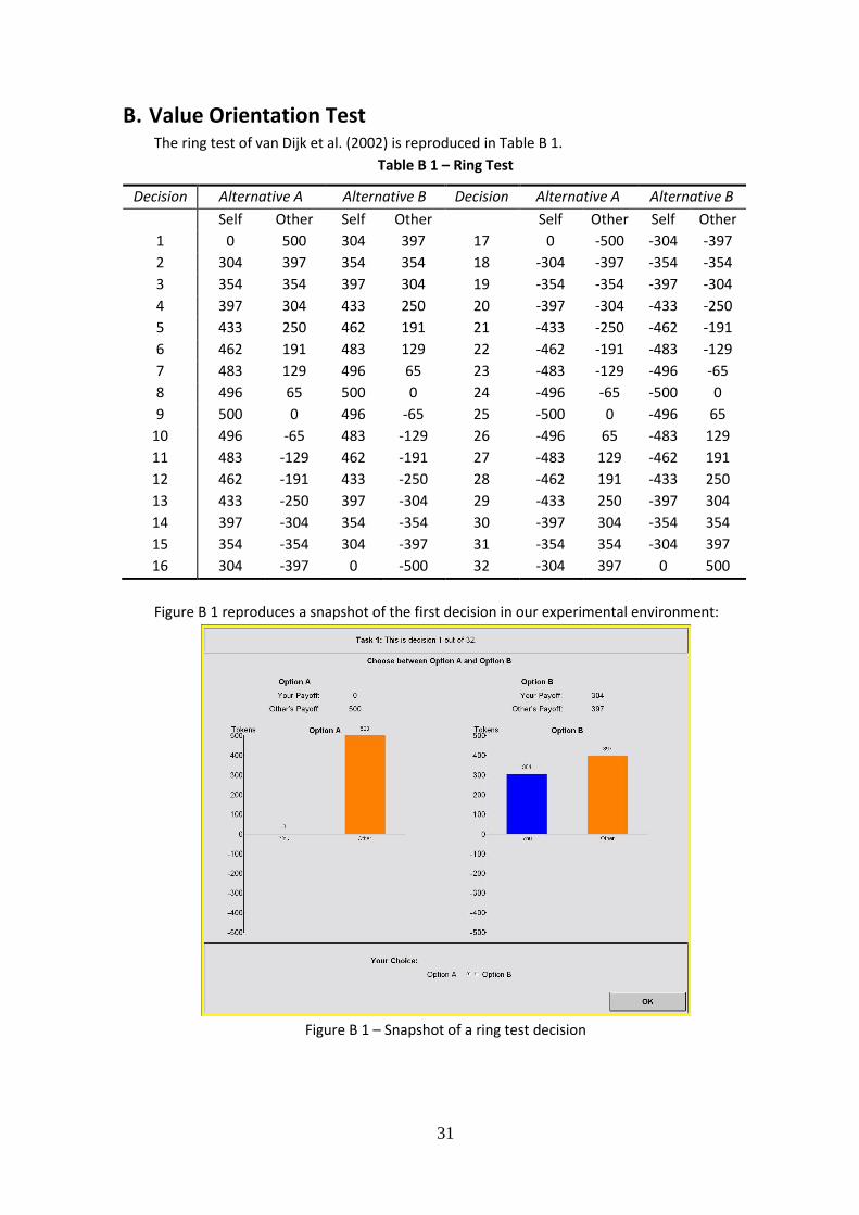
31

B. Value Orientation Test The ring test of van Dijk et al. (2002) is reproduced in Table B 1.

Table B 1 – Ring Test

Decision Alternative A Alternative B Decision Alternative A Alternative B Self Other Self Other

Self Other Self Other

1 0 500 304 397 17 0 -500 -304 -397

2 304 397 354 354 18 -304 -397 -354 -354

3 354 354 397 304 19 -354 -354 -397 -304

4 397 304 433 250 20 -397 -304 -433 -250

5 433 250 462 191 21 -433 -250 -462 -191

6 462 191 483 129 22 -462 -191 -483 -129

7 483 129 496 65 23 -483 -129 -496 -65

8 496 65 500 0 24 -496 -65 -500 0

9 500 0 496 -65 25 -500 0 -496 65

10 496 -65 483 -129 26 -496 65 -483 129

11 483 -129 462 -191 27 -483 129 -462 191

12 462 -191 433 -250 28 -462 191 -433 250

13 433 -250 397 -304 29 -433 250 -397 304

14 397 -304 354 -354 30 -397 304 -354 354

15 354 -354 304 -397 31 -354 354 -304 397

16 304 -397 0 -500 32 -304 397 0 500

Figure B 1 reproduces a snapshot of the first decision in our experimental environment:

Figure B 1 – Snapshot of a ring test decision

32

C. Auxiliary Tables

Table C 1 presents the input of subjects on the motivations of different strategies in the

participation game. This information was collected in the post-experiment questionnaire. Note

that the available options correspond to motivations that have a rough correspondence to our

preference specification: (α=0), competitive (α<0), in-group co-operator (α>0, β>γ), overall co-

operator (α>0, β=γ).

Table C 1 - Reported motivations in the questionnaire

Main goal of a participant who… …participated most

of the times.

…did not participate

most of the times.

Make as much money as possible for himself

or herself. 27.50% 77.50%

Increase the difference between his or her

earnings and the earnings of other

participants.

1.88% 20.00%

Help his or her group make as much money as

possible. 63.75% 1.25%

Help both his or her group and the other

group make as much money as possible. 6.88% 1.25%

Table C 2 presents OLS regression results on the relationship between personality traits and

participation behavior, and between personality traits and other-regarding preferences.

Table C 2 - Participation, personal traits, and value orientation

Average Participation Altruism (motivational

vector’s angle)

Agreeableness -.0608* 0.080

(-1.71) (0.03)

Conscientiousness .007 2.167

(0.24) (0.93)

Extraversion .029 -2.539

(0.93) (-1.09)

Openness -.056 0.449

(-1.64) (0.19)

Neuroticism .007 -2.321

(0.22) (-0.90)

Altruism (motivational vector’s

angle)

.003**

(3.02)

Constant .975** 16.196

(4.38) (0.98)

R2 0.11 0.02

OLS regression. N=152. t-statistics in parentheses. * (**) indicates significance at the 10% (1%)

level.

33

Table C 3 (left-hand side panel) shows average scores on the in-group bias measures separately

for individuals with high and low in-group bias. The right-hand side panel presents the same

results for individuals whose group won the quiz between laboratories and those who lost the

quiz.

Table C 3 - In-group bias, openness, and uiz utcome.

In-group bias Low Openness High Openness Lost Quiz Won Quiz

Average of 1st and 2nd

allocation

101.2

(94.5)

95.5

(92.5)

110.2

(96.1)

95.4

(90.9)

1st allocation (before PG) 92.7

(99.5)

109.2

(95.4)

112.4

(99.6)

97.4

(96.8)

2nd allocation (after PG) 109.7

(117.2)

81.8

(131.4)

108.0

(127.7)

93.4

(119.3)

Stated 3.6

(3.3)

2.5

(3.8)

3.1

(3.5)

3.2

(2.9)

N 76 76 57 55

Each cell presents the mean and standard deviation (in parentheses). Low (High) openness: bottom- (top-

) 10 openness. Note that Control subjects are not included in the right-hand side panel, as this treatment

does not include the quiz tournament. Using Mann-Whitney tests, we find no statistically significant

differences (at the 5% level) across openness.

Table C 4 presents OLS regression results on the relationship between average individual

participation and a linear trend, for each motivational category. Table C 4 – Regression of Average Participation on a Linear Trend

Competitors Individualists Weak Altruists Mild Altruists Strong Altruists

Constant 0.682** 0.794** 0.845** 0.804** 0.734**

(34.42) (40.12) (30.58) (37.05) (23.83)

Linear Trend -0.601** -0.210* -0.373** -0.296** 0.150

(-7.21) (-2.49) (-3.21) (-3.21) (1.15)

R2 0.58 0.14 0.21 0.21 0.03

OLS regression, N=152. t-statistics in parentheses. * (**) indicates significance at the 10% (1%) level.

Linear trend coefficients multiplied by 102.

34

Table C 5 presents model specifications that supplement the results presented in Table 3.

Table C 5 – Robustness checks

1 2 3

Motivational Vector 0.022*** 0.006 0.038***

(2.74) (0.62) (3.12)

In-group bias 0.980* 0.984* 1.008* (1.72) (1.71) (1.78) High 1.096** 1.097** 1.137** (2.07) (2.07) (2.16) Low 0.397 0.399 0.424 (0.89) (0.89) (0.96) Trend -0.032*** -0.038*** -0.039*** (2.66) (3.13) (3.22) Trend2 0.000 0.000 0.000 (1.19) (1.21) (1.28) In-group bias*High -1.336* -1.339* -1.401* (1.72) (1.72) (1.82) In-group bias*Low -0.961 -0.966 -1.037 (1.31) (1.31) (1.42) Strong Altruist -1.599*** (3.00) Strong Altruist * Trend 0.035*** (4.62) Motivational Vector * Trend 0.001*** (4.46) Constant 1.083*** 1.204*** 1.253*** (2.99) (3.30) (3.46)

Notes: N=152. Cells present the logit estimation (with random effects at the individual level); N=152. High and Low are dummy treatment variables. In-group bias is measured as the average of the two dictator allocation decisions, re-scaled to the interval [-1,1]. Strong Altruist is a type dummy. Absolute z-scores in parentheses. * (**, ***) indicates significance at the 10% (5%, 1%) level.

D. Other-regarding Preferences and In-group bias In this Appendix, we examine the relationship between altruism and in-group bias. In other

words, we are interested in whether distinct motivational types respond differently to in-group

bias manipulations. For this purpose, Figure D 1 shows the average percentages of the

endowment allocated to the in-group member – both before and after the participation game –

per motivational category and treatment.

Consider first the average in-group bias across treatments. Individualists are the category

showing the highest in-group bias, with an average allocation of 79,1% of the endowments to

the in-group. The group showing the lowest in-group bias are Competitors, for whom the

average allocation to the in-group member is 67.4%. Despite the apparent diversity in allocation

behavior, the only significant difference across categories when using the average of the two

decisions is between Competitors and Individualists (MW, p=0.05). A Pearson's chi-square test

corroborates this point: there is no significant systematic difference over categories for the

average of the two decisions, neither across all treatments, nor for any particular treatment (all

p>0.35). In the allocation decision before the participation game, the bias is stronger for

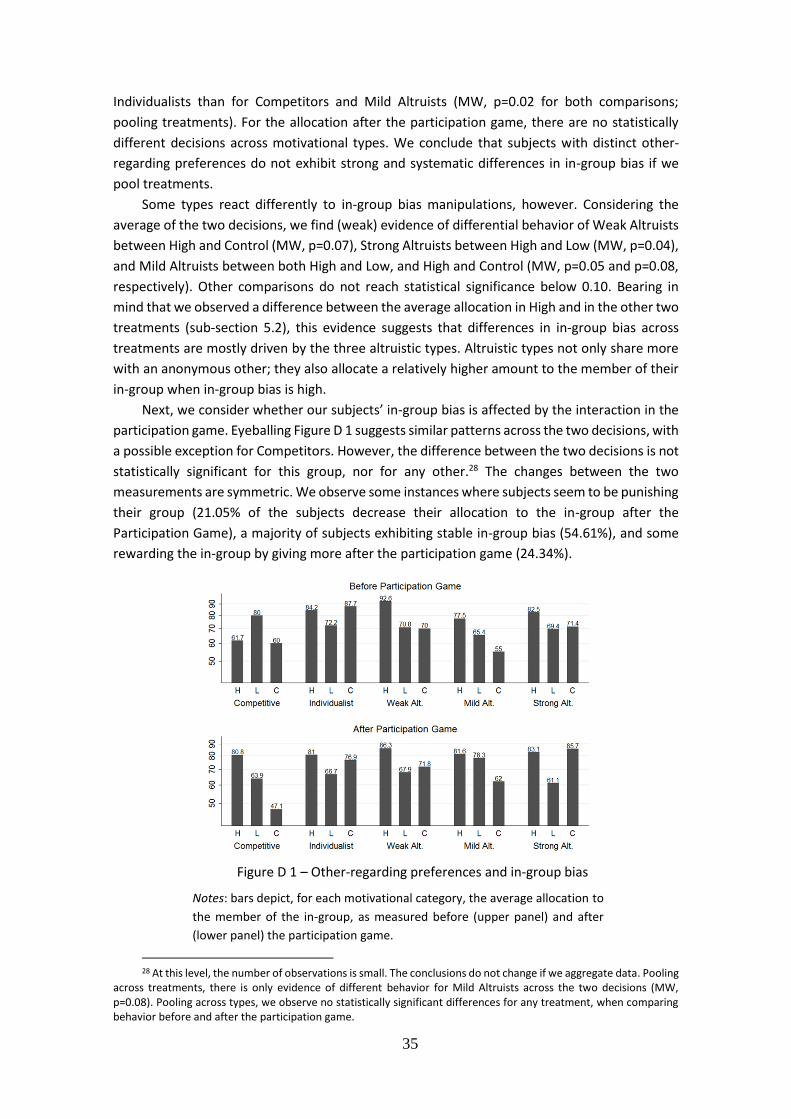
35

Individualists than for Competitors and Mild Altruists (MW, p=0.02 for both comparisons;

pooling treatments). For the allocation after the participation game, there are no statistically

different decisions across motivational types. We conclude that subjects with distinct other-

regarding preferences do not exhibit strong and systematic differences in in-group bias if we

pool treatments.

Some types react differently to in-group bias manipulations, however. Considering the

average of the two decisions, we find (weak) evidence of differential behavior of Weak Altruists

between High and Control (MW, p=0.07), Strong Altruists between High and Low (MW, p=0.04),

and Mild Altruists between both High and Low, and High and Control (MW, p=0.05 and p=0.08,

respectively). Other comparisons do not reach statistical significance below 0.10. Bearing in

mind that we observed a difference between the average allocation in High and in the other two

treatments (sub-section 5.2), this evidence suggests that differences in in-group bias across

treatments are mostly driven by the three altruistic types. Altruistic types not only share more

with an anonymous other; they also allocate a relatively higher amount to the member of their

in-group when in-group bias is high.

Next, we consider whether our subjects’ in-group bias is affected by the interaction in the

participation game. Eyeballing Figure D 1 suggests similar patterns across the two decisions, with

a possible exception for Competitors. However, the difference between the two decisions is not

statistically significant for this group, nor for any other.28 The changes between the two

measurements are symmetric. We observe some instances where subjects seem to be punishing

their group (21.05% of the subjects decrease their allocation to the in-group after the

Participation Game), a majority of subjects exhibiting stable in-group bias (54.61%), and some

rewarding the in-group by giving more after the participation game (24.34%).

28 At this level, the number of observations is small. The conclusions do not change if we aggregate data. Pooling

across treatments, there is only evidence of different behavior for Mild Altruists across the two decisions (MW, p=0.08). Pooling across types, we observe no statistically significant differences for any treatment, when comparing behavior before and after the participation game.

Figure D 1 – Other-regarding preferences and in-group bias

Notes: bars depict, for each motivational category, the average allocation to

the member of the in-group, as measured before (upper panel) and after

(lower panel) the participation game.

36

E. Experimental Instructions In this Appendix, we reproduce the experiment’s instructions. Italicized text corresponds

to text that was part of High and Low, but not Control. Text within square brackets was not part

of the instructions, but is included to clarify the experimental protocol. Trivia questions and

other non-reproduced details are available upon request. We also provide the post-experiment

questionnaire.

Welcome to this experiment in decision-making. Depending on your decisions and the decisions of

other subjects you may earn money. You will be paid privately at the end of the session. This is an

anonymous experiment: your identity will not be revealed to other participants. The choices you make in

early parts of the experiment may be used in later parts. Since this experiment involves gains and losses,

it is possible (though very unlikely) that you make a negative amount in the experiment. In that case, your

earnings will be deducted from the show-up fee. It is not possible that your losses exceed the show-up

fee. This experiment is composed of three main tasks: Task 1, Task 2, and Task 3. You will receive

instructions for a new task after the previous one has been completed. Note that a new task will only

begin when every participant has finished the previous one.

Ring Test: In Task 1 you will be asked to make 32 decisions with monetary consequences. In each of

the 32 situations you will have to choose between two options: Option A and Option B. For each option,

two numbers will be displayed. The first is the number of tokens that you yourself will receive (positive

amounts) or pay (negative amounts). The second is the number of tokens that the "Other" will receive or

pay as a consequence of your decision. The "Other" is an anonymous person in this room, with whom you

are randomly matched for the entire duration of Task 1. You will also be randomly matched with a second,

different anonymous participant whose choices will affect you in the same way that your choices affect

the "Other". Note: this means that the person who receives or loses money due to your decisions is a

different person than the one whose decisions make you earn or lose money.

Your total payoff is the result of both your decisions and the decisions made by the participant whose

choices affect you. No participant will know with whom he or she has been paired. Participants will only

be informed about the total amount they earned or lost at the end of the experiment.

BFI: In Task 2 you will be asked to rate a number of characteristics that may or may not apply to you.

There are 44 statements in total, distributed over 4 screens. Please pick a number from 1 to 5 next to each

statement to indicate the extent to which you agree or disagree with that statement. Most people take

no more than 10 minutes to complete this task.

The Openness Score: The statements you rated in Task 2 constitute a self-report inventory of

personality traits (characteristics). We employed one of the most used and reliable personality trait tests.

One of the traits that was measured is 'Openness', whose score can range from 1 to 5.

What is Openness?: Openness is a personality trait that involves active imagination, aesthetic

sensitivity, attentiveness to inner feelings, preference for variety, and intellectual curiosity. It captures

receptivity to novel experiences and ideas. It is not the cultural habits and knowledge acquired through

education or breeding, nor is it related to intelligence or any other cognitive ability.

People whose Openness Score lies more to the left-hand side of the scale:

- tend to be more conventional and traditional in their opinions and behavior.

- prefer familiar routines to new experiences.

- generally focus on a narrower range of interests.

- are practical and down-to-earth.

- are able to more easily separate ideas from feelings.

People whose Openness Score lies more to the right-hand side of the scale

- are curious, open to unknown things and variety.

- are frequently described as imaginative, artistic, unconventional and tolerant.

37

- are more willing to accept the validity of astrology and esoteric phenomena.

- have more easily access to thoughts and feelings simultaneously, thus experiencing things more

intensely.

We have constructed a ranking of the Openness Scores of the twenty participants of this experiment.

This ranking ranges from 1 to 20, with 1 being the participant with the Openness Score more to the right,

and 20 the participant with the Openness Score more to the left.

We would like to ask the ten participants with rankings 1 to 10 to move to another lab. Please wait

for the organizers' instructions to do so. The other ten participants can remain seated. Given your ranking,

we would kindly ask you to prepare to move to the other lab/remain seated.

[Subjects are asked to stand up and move to new computer stations]

For the next 3 minutes, we would like the participants in each lab to pick a name to identify their lab.

We provide you with three pre-defined possibilities. You can discuss this with the other participants in the

same lab as you by using the chat box below.

Each participant submits his preferred choice, and the most picked choice will be the name that will

identify your lab for the remainder of the experiment.

Trivia Challenge: The participants in [name of the participant’s lab] and [name of the other lab] will

now compete in a trivia challenge. Each participant will be asked five trivia questions. You have 30 seconds

to answer each question. You cannot answer after time is up. Each correct answer corresponds to one

point, an incorrect answer corresponds to zero points. In the end, the points of all participants in [name of

the participant’s lab] will be summed, and compared to the total number of points achieved by the

participants in [name of the other lab]. The lab with more points gets a total reward of 2000 tokens (10

Euros), to be equally distributed among all participants of the winning lab, i.e. each participant gets 200

tokens (1 Euro). In case the two labs achieve the same number of points, the winner is decided randomly

(with equal probability).

First Allocation Decision: We would like to ask you to divide 200 tokens (1 Euro) between a random

participant who is part of your group (excluding yourself) and a random participant who is part of the

other group. Recall that your group is composed of you and 4 other participants from [name of the

participant’s lab]. The other group is composed of 5 participants from [name of the other/the participant’s

lab in High/Low, respectively].

These amounts will be paid at the end of the experiment. We will randomly select both a member

of your group and a member of the other group who will receive your chosen allocation. You will be

affected by the choices of two other random participants in the same way.

Participation Game: In Task 3 you will be asked to make decisions in 40 rounds, with one decision

per round. You will be part of a group of 5 participants: you and 4 others. The participants that are part

of your group are all drawn from [name of the participant’s lab]. Group composition will remain constant

for the whole of Task 3. Your group will interact with another group of 5 participants, all of them drawn

from [name of the other/the participant’s lab in High/Low, respectively].

In every round, each member of a group will have to decide on whether to buy a "disc" or not. A

"disc" costs 30 tokens. Members of the group with more "discs" receive a higher reward: 120 tokens.

Members of the group with fewer "discs" receive a lower reward: 30 tokens.

If the number of discs in the two groups is the same, the group who gets the higher reward in that

round is picked with equal probability. In other words, in case of a tie each group has a 50% chance of

getting the high reward. Note that if one of the groups gets the high reward the other necessarily gets the

low reward.

As an example, assume that 3 people in your group buy discs, but only 2 people in the other group

buy discs. In this situation, your group gets the high reward in this round. A member of your group who

bought a disc gets a payoff of 90 tokens in this round. A member of your group who did not buy a disc

gets a payoff of 120 tokens in this round. A member of the other group who bought a disc gets a payoff

of 0 tokens in this round. A member of the other group who did not buy a disc gets a payoff of 30 tokens

in this round.

38

Second Allocation Decision: [identical to the First Allocation Decision.]

Post-experiment Questionnaire

1. Can you please briefly describe what you did in the disc-buying part of the experiment and why

you did it.

2. How attached did you feel towards your group on a scale from 1 (not at all) to 10 (very much)?

3. How attached did you feel towards the other group on a scale from 1 (not at all) to 10 (very

much)?

4. In your opinion, the main goal of a participant who bought many discs was to:

Make as much money as possible for himself or herself.

Increase the difference between his or her earnings and the earnings of other

participants.

Help his or her group make as much money as possible.

Help both his or her group and the other group make as much money as possible.

5. In your opinion, the main goal of a participant who bought few discs was to:

Make as much money as possible for himself or herself.

Increase the difference between his or her earnings and the earnings of other

participants.

Help his or her group make as much money as possible.

Help both his or her group and the other group make as much money as possible.