other common univariate distributions - stony brookzhu/ams570/lecture6_570.pdf · 2018-02-13 ·...
TRANSCRIPT
1
Other Common Univariate Distributions
Dear students, besides the Normal, Bernoulli and Binomial
distributions, the following distributions are also very
important in our studies.
1. Discrete Distributions
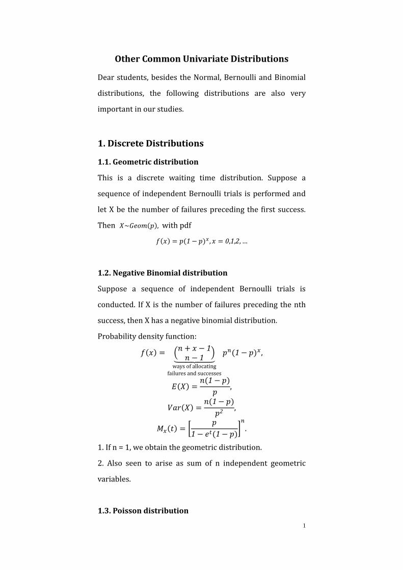
1.1. Geometric distribution
This is a discrete waiting time distribution. Suppose a
sequence of independent Bernoulli trials is performed and
let X be the number of failures preceding the first success.
Then 𝑋~𝐺𝑒𝑜𝑚(𝑝), with pdf
𝑓(𝑥) = 𝑝(1− 𝑝)𝑥 , 𝑥 = 0,1,2, …
1.2. Negative Binomial distribution
Suppose a sequence of independent Bernoulli trials is
conducted. If X is the number of failures preceding the nth
success, then X has a negative binomial distribution.
Probability density function:
𝑓(𝑥) = (𝑛 + 𝑥 − 1𝑛 − 1
)⏟
ways of allocatingfailures and successes
𝑝𝑛(1− 𝑝)𝑥,
𝐸(𝑋) =𝑛(1− 𝑝)
𝑝,
𝑉𝑎𝑟(𝑋) =𝑛(1− 𝑝)
𝑝2,
𝑀𝑥(𝑡) = [𝑝
1− 𝑒𝑡(1− 𝑝)]𝑛
.
1. If n = 1, we obtain the geometric distribution.
2. Also seen to arise as sum of n independent geometric
variables.
1.3. Poisson distribution

2
Parameter: rate 𝜆 > 0
MGF: 𝑀𝑥(𝑡) = 𝑒𝜆(𝑒𝑡−1)
Probability density function:
𝑓(𝑥) =𝑒−𝜆𝜆𝑥
𝑥!, 𝑥 = 0,1,2, …
1. The Poisson distribution arises as the distribution for the
number of “point events” observed from a Poisson process.
Examples:
Figure 1: Poisson Example
2. The Poisson distribution also arises as the limiting form
of the binomial distribution:
𝑛 → ∞, 𝑛𝑝 → 𝜆
𝑝 → 0
The derivation of the Poisson distribution (via the binomial)
is underpinned by a Poisson process i.e., a point process on
[0,∞); see Figure 1.
AXIOMS for a Poisson process of rate λ > 0 are (That is, a
counting process is a Poisson process if it satisfies the
following rules):
(A) The number of occurrences in disjoint intervals are
independent.
(B) Probability of exactly 1 occurrence in any sub-interval
[𝑡, 𝑡 + h) is 𝜆h+ 𝑜(h) (h → 0) (approx prob. is equal to
length of interval (h) times 𝜆).
(C) Probability of more than one occurrence in [𝑡, 𝑡 + h) is
𝑜(h) (h → 0) (i.e. prob is small, negligible).
Note: 𝑜(h) , pronounced (small order h) is standard

3
notation for any function 𝑟(ℎ) with the property:
𝑙𝑖𝑚ℎ→0
𝑟(ℎ)
ℎ= 0
1.4. Hypergeometric distribution
Consider an urn containing M black and N white balls.
Suppose n balls are sampled randomly without replacement
and let X be the number of black balls chosen. Then X has a
hypergeometric distribution.
Parameters: 𝑀,𝑁 > 0, 0 < 𝑛 ≤ 𝑀 + 𝑁
Possible values: 𝑚𝑎𝑥 (0, 𝑛 − 𝑁) ≤ 𝑥 ≤ 𝑚𝑖𝑛 (𝑛,𝑀)
Prob. density function:
𝑓(𝑥) =(𝑀𝑥) (
𝑁𝑛 − 𝑥
)
(𝑀 + 𝑁𝑛
),
𝐸(𝑋) = 𝑛𝑀
𝑀 +𝑁, 𝑉𝑎𝑟(𝑋) =
𝑀 + 𝑁 − 𝑛
𝑀 + 𝑁 − 1
𝑛𝑀𝑁
(𝑀 + 𝑁)2.
The mgf exists, but there is no useful expression available.
1. The hypergeometric PDF is simply
# samples with x black balls
# possible samples
=(𝑀𝑥) (
𝑁𝑛 − 𝑥
)
(𝑀 + 𝑁𝑛
),
2. To see how the limits arise, observe we must have x ≤ n
(i.e., no more than sample size of black balls in the sample.)
Also, x ≤ M, i.e., x ≤ min (𝑛,𝑀).
Similarly, we must have x ≥ 0 (i.e., cannot have < 0 black
balls in sample), and
𝑛 − 𝑥 ≤ 𝑁 (i.e., cannot have more white balls than
number in urn).
i.e. 𝑥 ≥ 𝑛 − 𝑁
4
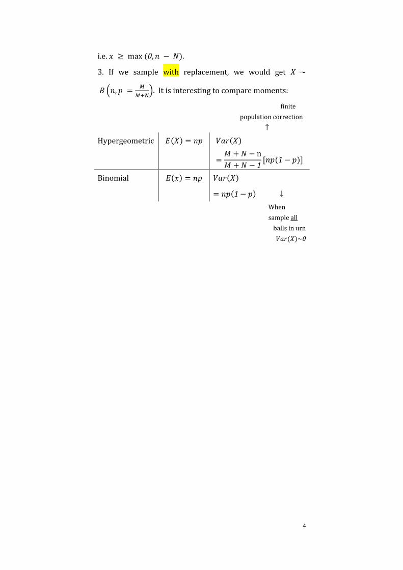
i.e. 𝑥 ≥ max (0, 𝑛 − 𝑁).
3. If we sample with replacement, we would get 𝑋 ∼
𝐵 (𝑛, 𝑝 =𝑀
𝑀+𝑁). It is interesting to compare moments:
finite
population correction
↑
Hypergeometric 𝐸(𝑋) = 𝑛𝑝 𝑉𝑎𝑟(𝑋)
=𝑀 + 𝑁 − n
𝑀 +𝑁 − 1[𝑛𝑝(1− 𝑝)]
Binomial 𝐸(𝑥) = 𝑛𝑝 𝑉𝑎𝑟(𝑋)
= 𝑛𝑝(1− 𝑝) ↓
When
sample all
balls in urn
𝑉𝑎𝑟(𝑋)~0

5
2. Continuous Distributions
2.1 Uniform Distribution
For 𝑋~ (𝑎, ), its pdf and cdf are:
𝑓(𝑥) = {
− 𝑎, 𝑎 < 𝑥 <
0, otherwise,
(𝑥) = ∫ 𝑓(𝑥) 𝑥 = ∫1
− 𝑎 𝑥 =
𝑥 − 𝑎
− 𝑎
𝑥
𝑥
−∞
,
or 𝑎 < 𝑥 <
The more complete form of the cdf is:
(𝑥) = {
0 𝑥 ≤ 𝑎𝑥 − 𝑎
− 𝑎 𝑎 < 𝑥 <
1 ≤ 𝑥
Its mgf is:
𝑀 (𝑡) =𝑒𝑡 − 𝑒𝑡
𝑡( − 𝑎)
A special case is the 𝑋~ (0,1) distribution:
𝑓(𝑥) = {1 0 < 𝑥 < 10 otherwise,
(𝑥) = 𝑥 for 0 < 𝑥 < 1
𝐸(𝑋) =1
2, 𝑉𝑎𝑟(𝑋) =
1
12, 𝑀(𝑡) =
𝑒𝑡 − 1
𝑡.
2.2 Exponential Distribution
PDF: 𝑓(𝑥) = 𝜆𝑒−𝜆𝑥, 𝑥 ≥ 0
CDF: (𝑥) = 1 − 𝑒−𝜆𝑥,
MGF:
𝑀 (𝑡) =𝜆
𝜆 − 𝑡, 𝜆 > 0, 𝑥 ≥ 0.
This is the distribution for the waiting time until the first
occurrence in a Poisson
process with rate parameter 𝜆 > 0.
1. If 𝑋~𝐸𝑥𝑝(𝜆) then,

6
𝑃(𝑋 ≥ 𝑡 + 𝑥|𝑋 ≥ 𝑡) = 𝑃(𝑋 ≥ 𝑥)
(memoryless property)
2. It can be obtained as limiting form of geometric
distribution.
3. One can also easily derive that the geometric distribution
also has the memoryless property.
2.3 Gamma distribution
~ ( , )X gamma
11if ( ) , 0
( )
x
f x x e x
Or, some books use 1
Then: 1( ) , 0( )
rr xf x x e x
r
If r is a non-negative integer, then ( ) ( 1)!r r
1
01 ( )
( )
rr xf x dx x e dx
r
1
0( ) r r xr x e dx
( ) 1
r r
X
t tM t
( )
r
XM tt
2
( )
( )
rE X
rVar X

7
Special case : when 21, ~
2 2k
kr X
Special case : when 1 ~ exp( )r X
Review ~ exp( )X
p.d.f. ( ) , 0xf x e x
m.g.f. ( )XM tt
e.g. Let . . .
~ exp( ) , 1, ,i i d
iX i n . What is the distribution of
1
n
i
i
X
?
Solution
1
( ) ( )ii
n
XXi
M t M t
n
t
~ ( , )iX gamma r n
e.g. Let 2~ kW . What is the mgf of W ?
Solution
21
2( )1
2
k
WM t
t
21( )
1 2
k
WM tt
e.g. Let 1
2
1 ~ kW , 2
2
2 ~ kW , and 1 2 and W W are independent.
What is the distribution of 1 2W W ?
Solution

8
1 2 1 2( ) ( ) ( )W W W WM t M t M t
1 2
2 21 1
1 2 1 2
k k
t t
1 2
21
1 2
k k
t
1 2
2
1 2 ~ k kW W
*** In general, for 𝑋 ∼ 𝑔amma(α, λ), α > 0.
(Note, sometimes we use r instead of α as shown above.)
1. α is the shape parameter,
𝜆 is the scale parameter
Note: if 𝑌 ∼ 𝑔amma (𝛼, 1) and 𝑋 =𝑌
𝜆, then 𝑋 ∼
𝑔amma(α, λ), That is, λ is scale parameter.
Figure 2: Gamma Distribution
2. Gamma (𝑘
2,1
2) distribution is also called χ𝑘
2 (chi-square
with 𝑘 df) distribution, if 𝑘 is a positive integer;
3. The 𝑔amma (𝐾, 𝜆) random variable can also be
interpreted as the waiting time until the 𝐾𝑡ℎ occurrences
(events) in a Poisson process.
2.4 Beta density function
Suppose Y1 ∼ Gamma (𝛼, 𝜆) , 𝑌2 ∼ Gamma (β, λ)
independently, then,
X =𝑌1
𝑌1 + 𝑌2~𝐵(𝛼, 𝛽), 0 ≤ 𝑥 ≤ 1.
Remark: we have derived this in Lecture 5 – transformation.

9
I have copied it here again, as a review.
e.g. Suppose that 𝑌1~ gamma(α, 1), 𝑌2~ gamma(β, 1),
and that 𝑌1 and 𝑌2 are independent. Define the
transformation
1 = 𝑔1(𝑌1, 𝑌2) = 𝑌1 + 𝑌2
2 = 𝑔2(𝑌1, 𝑌2) =𝑌1
𝑌1 + 𝑌2.
Find each of the following distributions: (a) 𝑓𝑈1,𝑈2(𝑢1, 𝑢2), the joint distribution of 1and 2,
(b) 𝑓𝑈1(𝑢1), the marginal distribution of 1, and
(c) 𝒇𝑼𝟐(𝒖𝟐), the marginal distribution of 𝑼𝟐.
Solutions. (a) Since 𝑌1 and 𝑌2 are independent, the joint
distribution of 𝑌1 and 𝑌2 is 𝑓𝑌1,𝑌2(𝑦1, 𝑦2) = 𝑓𝑌1(𝑦1)𝑓𝑌2(𝑦2)
=
Γ(𝛼)𝑦1𝛼−1𝑒−𝑦1
×
Γ(𝛽)𝑦2𝛽−1𝑒−𝑦2
=
Γ(𝛼)Γ(𝛽)𝑦1𝛼−1𝑦2
𝛽−1𝑒−(𝑦1+𝑦2),
for 𝑦1 > 0, 𝑦2 > 0, and 0, otherwise. Here, 𝑅𝑌1,𝑌2 =
{(𝑦1, 𝑦2): 𝑦1 > 0, 𝑦2 > 0}. By inspection, we see that
𝑢1 = 𝑦1 + 𝑦2 > 0, and 𝑢2 =𝑦1
𝑦1+ 𝑦2 must fall between 0 and
1.
Thus, the domain of 𝑼 = ( 1, 2) is given by 𝑅𝑈1,𝑈2 = {(𝑢1, 𝑢2): 𝑢1 > 0, 0 < 𝑢2 < }.
The next step is to derive the inverse transformation. It
follows that
𝑢1 = 𝑦1 + 𝑦2
𝑢2 =𝑦1
𝑦1 + 𝑦2
⇒𝑦1 = 𝑔1
−1(𝑢1, 𝑢2) = 𝑢1𝑢2𝑦2 = 𝑔2
−1(𝑢1, 𝑢2) = 𝑢1 − 𝑢1𝑢2
The Jacobian is given by
𝐽 = det ||
𝜕𝑔1−1(𝑢1, 𝑢2)
𝜕𝑢1
𝜕𝑔1−1(𝑢1, 𝑢2)
𝜕𝑢2𝜕𝑔2
−1(𝑢1, 𝑢2)
𝜕𝑢1
𝜕𝑔2−1(𝑢1, 𝑢2)
𝜕𝑢2
|| = det |
𝑢2 𝑢1 − 𝑢2 −𝑢1
|
= −𝑢1𝑢2 − 𝑢1( − 𝑢2) = −𝑢1.
We now write the joint distribution for 𝑼 = ( 1, 2). For
𝑢1 > 0 and 0 < 𝑢2 < , we have that 𝑓𝑈1,𝑈2(𝑢1, 𝑢2)
= 𝑓𝑌1,𝑌2[𝑔1−1(𝑢1, 𝑢2), 𝑔2
−1(𝑢1, 𝑢2)]|𝐽|

10
=
Γ(𝛼)Γ(𝛽)(𝑢1𝑢2)
𝛼−1(𝑢1 − 𝑢1𝑢2)𝛽−1𝑒−[(𝑢1𝑢2)+(𝑢1−𝑢1𝑢2)]
× | − 𝑢1|
Note: We see that 1and 2 are independent since the domain 𝑅𝑈1,𝑈2 = {(𝑢1, 𝑢2): 𝑢1 > 0, 0 < 𝑢2 < } does not
constrain 𝑢1 by 𝑢2 or vice versa and since the nonzero
part of 𝑓𝑈1,𝑈2(𝑢1, 𝑢2) can be factored into the two expressions
ℎ1(𝑢1) and ℎ2(𝑢2), where
ℎ1(𝑢1) = 𝑢1𝛼+𝛽−1𝑒−𝑢1
and
ℎ2(𝑢2) =𝑢2𝛼−1( − 𝑢2)
𝛽−1
Γ(𝛼)Γ(𝛽).
(b) To obtain the marginal distribution of 1, we integrate the joint pdf𝑓𝑈1,𝑈2(𝑢1, 𝑢2)
over 𝑢2. That is, for 𝑢1 > 0,
𝑓𝑈1(𝑢1) = ∫ 𝑓𝑈1,𝑈2(𝑢1, 𝑢2)1
𝑢2=0
𝑢2
= ∫𝑢2𝛼−1( − 𝑢2)
𝛽−1
Γ(𝛼)Γ(𝛽)𝑢1𝛼+𝛽−1𝑒−𝑢1
1
𝑢2=0
𝑢2
=
Γ(𝛼)Γ(𝛽)𝑢1𝛼+𝛽−1𝑒−𝑢1∫ 𝑢2
𝛼−1( 1
𝑢2=0
− 𝑢2)𝛽−1 𝑢2
(𝑢2𝛼−1(1−𝑢2)
𝛽−1 is beta(𝛼,𝛽) kernel)⇔
Γ(𝛼)Γ(𝛽)𝑢1𝛼+𝛽−1𝑒−𝑢1
×Γ(𝛼)Γ(𝛽)
Γ(𝛼 + 𝛽)
=
Γ(𝛼 + 𝛽)𝑢1𝛼+𝛽−1𝑒−𝑢1
Summarizing,
𝑓𝑈1(𝑢1) = {
Γ(𝛼 + 𝛽)𝑢1𝛼+𝛽−1𝑒−𝑢1 , 𝑢1 > 0
0, otherwise.
We recognize this as a gamma( 𝛼 + 𝛽, 1) pdf; thus,
marginally, 1 ~gamma(𝛼 + 𝛽, 1).
(c) To obtain the marginal distribution of 2, we integrate the joint pdf 𝑓𝑈1,𝑈2(𝑢1, 𝑢2) over 𝑢2. That is, for 0 < 𝑢2 < ,
𝑓𝑈2(𝑢2) = ∫ 𝑓𝑈1,𝑈2(𝑢1, 𝑢2)∞
𝑢1=0
𝑢1

11
= ∫𝑢2𝛼−1( − 𝑢2)
𝛽−1
Γ(𝛼)Γ(𝛽)𝑢1𝛼+𝛽−1𝑒−𝑢1
∞
𝑢1=0
𝑢1
=𝑢2𝛼−1( − 𝑢2)
𝛽−1
Γ(𝛼)Γ(𝛽)∫ 𝑢1
𝛼+𝛽−1𝑒−𝑢1∞
𝑢1=0
𝑢1
=Γ(𝛼 + 𝛽)
Γ(𝛼)Γ(𝛽)𝑢2𝛼−1( − 𝑢2)
𝛽−1.
Summarizing,
𝑓𝑈2(𝑢2) = {
Γ(𝛼 + 𝛽)
Γ(𝛼)Γ(𝛽)𝑢2𝛼−1( − 𝑢2)
𝛽−1, 0 < 𝑢2 <
0, otherwise.
Thus, marginally, U2 ~ beta(𝜶,𝜷). □
Figure. Selected Beta pdf ’s
(https://en.wikipedia.org/wiki/Beta_distribution).
2.5 Standard Cauchy distribution
Possible values: 𝑥 ∈ 𝑅

12
PDF: 𝑓(𝑥) =1
𝜋(
1
1+𝑥2) ; (location parameter 𝜃 = 0)
CDF: (𝑥) =1
2+
1
𝜋arctan𝑥
𝐸(𝑋), 𝑉𝑎𝑟(𝑋),𝑀 (𝑡) do not exist.
The Cauchy is a bell-shaped distribution symmetric about
zero for which no moments are defined.
If 𝑍1 ∼ 𝑁(0, 1) and 𝑍2 ∼ 𝑁(0, 1) independently, then
𝑋 =𝑍1
𝑍2~Cauthy distribution. Please also see the lecture
notes on transformation for proof (Lecture 5).
HW4: 3.2, 3.5, 3.7, 3.9, 3.12, 3.18, 3.23

13
HW3 Q.1. Suppose that 𝒀𝟏 and 𝒀𝟐 are random variables
with joint pdf
𝒇𝒀𝟏,𝒀𝟐(𝒚𝟏, 𝒚𝟐) = {𝟖𝒚𝟏𝒚𝟐, 𝟎 < 𝒚𝟏 < 𝒚𝟐 < 𝟏𝟎, 𝐨𝐭𝐡𝐞𝐫𝐰𝐢𝐬𝐞.
Find the pdf of 𝑼𝟏 = 𝒀𝟏/𝒀𝟐.
It is given that the joint pdf of 𝑋 and 𝑌is 𝑓𝑌1,𝑌2(𝑦1, 𝑦2) =
8𝑦1𝑦2, 0 < 𝑦1 < 𝑦2 < .
Now we need to introduce a second random variable 2 which
is a function of 𝑋 and 𝑌. We wish to do so in a way that the
resulting bivariate transformation is one-to-one and our task of
finding the pdf of 1 is as easy as possible. Our choice of
2 is of course, not unique. Let us define 2 = 𝑌2. Then the
transformation is:
𝑌1 = 1 ∗ 2
𝑌2 = 2
From this, we find the Jacobian:
J = |𝑢2 𝑢10
| = 𝑢2
To determine 𝑡ℎ𝑒 𝑛𝑒𝑤 𝑗𝑜𝑖𝑛𝑡 𝑜𝑚𝑎𝑖𝑛 ℬ, of 1and 2, we note
that
0 < 𝑦1 < 𝑦2 < ⇒ 0 < 𝑢1 ∗ 𝑢2 < 𝑢2 < , equivalently,
𝑢1 > 0
𝑢1 <
𝑢2 > 0
𝑢2 <
So ℬ is as indicated in the diagram below.
𝑓𝑈1,𝑈2(𝑢1, 𝑢2) = 8 ∗ (𝑢1 ∗ 𝑢2) ∗ 𝑢2 ∗ 𝑢2 = 8𝑢1𝑢23,
Thus, the marginal pdf of 1 is obtained by integrating
𝑓𝑈1,𝑈2(𝑢1, 𝑢2) with respect to𝑢2, yielding
𝑓𝑈1(𝑢1) = ∫ 8𝑢1𝑢231
0 𝑢2 = 2 ∗ 𝑢1, 0 < 𝑢1 < .