OTC 16845

Centrifuge Model Tests on Anchor Piles for Tension Leg Platforms E. H. Doyle, Consultant; E.T.R. Dean, Soil Models Limited; J. S. Sharma, University of Saskatchewan; M. D. Bolton, University of Cambridge; A. J. Valsangkar, University of New Brunswick, J. S. Newlin, Shell International E&P Company

Copyright 2004, Offshore Technology Conference This paper was prepared for presentation at the Offshore Technology Conference held in Houston, Texas, U.S.A., 3–6 May 2004. This paper was selected for presentation by an OTC Program Committee following review of information contained in an abstract submitted by the author(s). Contents of the paper, as presented, have not been reviewed by the Offshore Technology Conference and are subject to correction by the author(s). The material, as presented, does not necessarily reflect any position of the Offshore Technology Conference or officers. Electronic reproduction, distribution, or storage of any part of this paper for commercial purposes without the written consent of the Offshore Technology Conference is prohibited. Permission to reproduce in print is restricted to an abstract of not more than 300 words; illustrations may not be copied. The abstract must contain conspicuous acknowledgment of where and by whom the paper was presented.

Abstract

Four centrifuge model tests were conducted to study the lateral response of large-diameter piles in clay subject to large lateral displacements. The objectives were to quantify the cyclic response for lateral loading of two closely-spaced piles loaded in line, and to establish the nature and the extent of any gap that may form between the piles and the soil as a result of static or cyclic loading. This paper describes the tests and the results, and shows how the results were used as part of the foundation design considerations for the URSA tension-leg platform..

Introduction One method to connect the tendons of Tension Leg Platforms (TLPs) to the foundation piles is to drive the piles with the tendon bottom receptacle attached to the piles. This method was first used on the Mars TLP (Garside et al., 1997). Because it is a free-head pile, this direct-connect method may result in lateral deflections that exceed the criteria on which RP2A (1993, 2000) is based (see Matlock, 1970). The lateral deflections for the lateral tests in soft clay at Sabine, for example, did not exceed about 20% of the pile diameter. In addition, the Mars design was conservatively designed by assuming that large lateral displacements would create a “gap” between the pile and surface soils. The gap was calculated as 4C/γ, where C was the soil strength and γ was the buoyant soil density. In order to study the potential for gap formation and to better understand the group behavior of piles under large lateral displacements, a centrifuge test program was undertaken at Cambridge University.

. References, tables and figures at end of paper

The URSA TLP in Mississippi Canyon Block 809 (Digre et al, 1999; Gatlin, 1999) and the properties from one of the geotechnical investigation sites conducted as part of the design process served as the prototype for the centrifuge tests. The centrifuge tests simulated the lateral response of a 100-inch diameter pile embedded to 200 ft in a soil that modeled the geotechnical strength properties from one of the Ursa site investigations. For the group piles, a spacing-to-diameter ratio (i.e., s/d ratio) of 3.08 was used. Beam-column analyses on the prototype pile using the Matlock criteria and expected maximum design loads were used to develop the model pile sizes and test parameters. The final prototype pile design used at Ursa, while close to the pile and soil studied in the centrifuge test program, did not exactly match the pile and soil used in the test program. The results of the test program, however, were assumed to be close enough to be applicable to typical Gulf of Mexico TLP direct-connect pile designs such as the Ursa TLP.

This paper reports selected results from four centrifuge model tests. The tests provide data of pile-head load-displacements, bending moments, inferred shear loads and inferred lateral pressures (p), and displacements (y) under monotonic and cyclic loading conditions. This paper compares results with API RP2A (1993, 2000) design criteria for lateral loading. The paper also includes design recommendations for laterally loaded piles with large displacement.

Centrifuge Experimental Setup Centrifuge modelling techniques are widely used for offshore and other civil engineering applications to provide information for design (Schofield, 1980; Craig, 1983; Craig et al, 1984, 1988; Springman, 1993; Taylor, 1994; Murff, 1996; Clukey and Phillips, 2002). These techniques are fundamentally better than “single gravity” tests because stress levels in a centrifuge model can be arranged to be the same as in the corresponding “prototype” or full-size foundation. This is particularly important for model testing of soil, whose behavior depends strongly on stress.

Figures 1 and 2 show the modeling arrangement used for the four tests. A clay sample was contained within a 850mm diameter cylindrical tub. The clay was consolidated in three layers, A, B, and C. Prior to each centrifuge test, each of one

2 OTC 16845

or two model piles was installed by augering a hole, then pushing the pile into the hole. Samples of the clay extracted from the hole were taken for moisture content determination. A beam and top plate system was assembled, including an electric motor arranged to apply lateral displacements to a carriage, which carried a loading block attached by links to the tops of the piles. Additional instrumentation (not shown) was connected including displacement transducers, a vane testing rig to measure soil strengths during the test, a CCTV system, and other devices.

Figure 3 shows the lateral loading arrangement in detail. Horizontal loads were applied to each pile at the level of the “load line”. In the two-pile tests, the piles were connected by pile-to-pile links as shown. The pile on the right was connected to the loading block. The links were instrumented with strain gauges calibrated to measure force. Two linear variable differential transformers (LVDTs) were used to measure lateral displacements and rotations. They were rigidly connected to the top beam of the plate system. Their spindles were held against an LVDT bearing plate that extended upwards from the cap of the pile on the right.

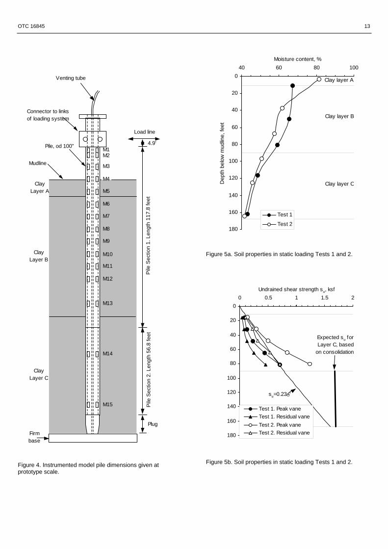
Figure 4 shows a typical pile with dimensions scaled to full-size or “prototype scale”. The pile was constructed from duraluminium in two sections of different internal diameters. The bottom of the pile was closed with a metal plug. The top included arrangements for connection to the loading system. A venting tube was provided down the centerline to assist with installation into the clay. A total of 15 strain-gauge systems M1−M15 were installed on the internal surfaces of each pile. Each gauge measured strain and was calibrated to measure bending moments in the pile.

Table 1 summarizes the four tests. All tests were at 100g centrifuge gravities. Test 1 was a static lateral loading test on a single pile, taken to failure. Test 2 was primarily a static loading test on two piles loaded in line, in the manner shown in Figure 1. The piles were spaced at 3.08 diameters from centerline to centerline. Some cyclic loading was done after the static test, but results are not reported here. Test 3 involved cyclic lateral loading of a single pile. Test 4 involved cyclic lateral loading of a two-pile group loaded in line. The piles were again at a spacing/diameter ratio of 3.08.

Table 2 lists the pile properties scaled to full-size or “prototype” scale. Macroscopic dimensions scale by the ratio N of centrifuge gravity to earth’s gravity, with N=100 for the present tests. All the piles tested were 1 inch od (outer diameter) at model scale, corresponding 100 inches od at prototype scale. Flexural rigidity EI scales with the fourth power of N, so prototype flexural rigidity was obtained by multiplying the value for the model pile by 1004. Because the pile was made of duraluminium while a typical TLP pile will be of steel, there is not a direct scaling of wall thickness. Instead, equivalent wall thicknesses are given in the table, such that a steel pipe of od 100” and equivalent wall thickness

will have a flexural rigidity 1004 times the flexural rigidity of the model pile.

Bending moments scale with the cube of N. The values of prototype bending moments at first yield have been obtained by computing the values for the model duraluminium pile whose stress at the elastic limit was taken as 34 ksi, and by then multiplying the results by 1003. The values of ultimate bending moments at prototype scale have been computed by multiplying the values for the model, based on an ultimate stress of 62 ksi for the duraluminium, and multiplying by 1003.

Table 3 lists properties of the speswhite kaolin clay used in the tests. The material was selected as being reasonably similar to “typical” Gulf of Mexico clays, and has been used on previous model tests, see for example Hamilton et al (1991), Murff and Hamilton (1993), Hamilton and Murff (1995), and others. For the present tests, mixing kaolin powder with de-ionized water under partial vacuum initially formed the clay. This produced a slurry at a moisture content of about twice the liquid limit. This was then poured and consolidated in the 850mm diameter steel tub at 1g in three layers, see Figure 1. Layer, C was consolidated to a uniform vertical effective stress of 7.3 ksf. To do this, the tub containing slurry was mounted into a “consolidometer” in which a piston applied a uniform total stress to the soil surface, with top and bottom drainage. The piston was removed. Slurry for layer B was poured onto the top of layer C. The layers were consolidated together by a downwards-hydraulic gradient method. In the present case the objective was to create a layer with a shear strength varying linearly with depth. Just before the first centrifuge test, layer A was poured as a slurry onto the top of layer B.

At the start of each centrifuge test, the 850mm diameter model container was loaded onto the centrifuge. The centrifuge gravity level was increased in stages to 100g, and the clay was allowed to re-consolidate at 100g for approximately 24 hours. Times for consolidation scale with N2, so the prototype consolidation period was around 1002 days, or approximately 27 years. Excess pore pressures were monitored using pore pressure transducers that had been installed in the clay during specimen preparation. In spite of the long consolidation time, full dissipation of excess pore pressures was not achieved, and in the first test the clay was under-consolidated − see below. After the consolidation period in each test, in-flight vane tests were carried out to measure the actual clay strengths achieved. Locations of the vane test sites are marked as V1, V2, V3 and V4 in Figure 2. At model scale, the vane was 0.55” high and 0.71” diameter. It was rotated at about 1° per second. The corresponding prototype values are 4.6 feet diameter, 5.9 feet high, and about 1° every 3 hours. After the vane tests had been carried out, the load test for the pile or pile group began.

At the end of each pile load test, the centrifuge was stopped and the steel tub was unloaded from the machine. The

OTC 16845 3

pile or piles for the test were carefully pulled out of the clay, and dummy piles were inserted in their place. The clay was then covered with cling film to prevent fluid entry, and the tub was stored until the next test. During the time between the end of one test and the beginning of the next, some swelling took place in the clay. The first action at the start of the next test was always to re-consolidate the clay to reverse this swelling. As a result of this, the clay increased in strength over the course of the centrifuge tests. Consequently, in comparing the results of different tests, it was necessary to take account of the different strengths as measured by the in-flight vane.

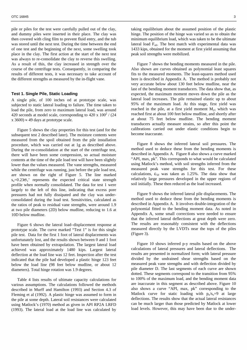
Test 1. Single Pile, Static Loading A single pile, of 100 inches od at prototype scale, was subjected to static lateral loading to failure. The time taken to load the pile, from zero to maximum lateral load, was around 420 seconds at model scale, corresponding to 420 x 1002 / (24 x 3600) ≈ 49 days at prototype scale.

Figure 5 shows the clay properties for this test (and for the subsequent test 2 described later). The moisture contents were measured from the spoil obtained from the pile installation procedure, which was carried out at 1g as described above. During the re-consolidation at the start of the centrifuge test, there will have been some compression, so actual moisture contents at the time of the pile load test will have been slightly lower than the values measured. The vane strengths, measured while the centrifuge was running, just before the pile load test, are shown on the right of Figure 5. The line marked su=0.23σv’ represents the expected critical state strength profile when normally consolidated. The data for test 1 were largely to the left of this line, indicating that excess pore pressures had not fully dissipated and the clay was under-consolidated during the load test. Sensitivities, calculated as the ratios of peak to residual vane strengths, were around 1.9 at two pile diameters (2D) below mudline, reducing to 1.6 at 10D below mudline.

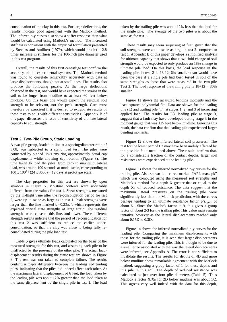
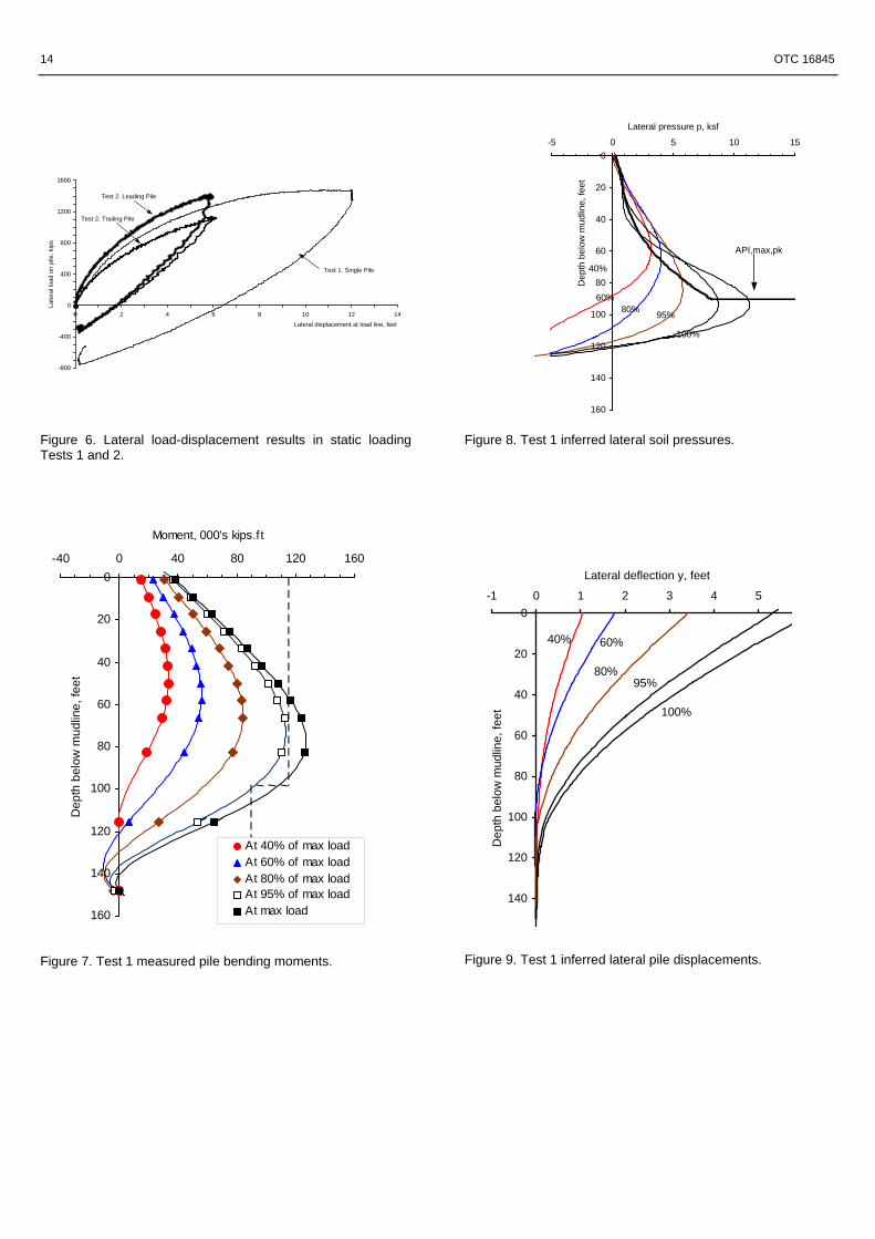
Figure 6 shows the lateral load−displacement response at prototype scale. The curve marked “Test 1” is for this single pile test. Data for the first 1 foot of lateral displacements was unfortunately lost, and the results shown between 0 and 1 foot have been obtained by extrapolation. The largest lateral load achieved was approximately 1480 kips. Largest lateral deflection at the load line was 12 feet. Inspection after the test indicated that the pile had developed a plastic hinge 123 feet below the load line (98 feet below mudline, or about 12 diameters). Total hinge rotation was 1.9 degrees.

Table 4 lists results of ultimate capacity calculations for various assumptions. The calculations followed the methods described in Murff and Hamilton (1993) and Section 4.3 of Fleming et al (1992). A plastic hinge was assumed to form in the pile at some depth. Lateral soil resistances were calculated using Matlock’s (1970) method as given in API RP2A LRFD (1993). The lateral load at the load line was calculated by

taking equilibrium about the assumed position of the plastic hinge. The position of the hinge was varied so as to obtain the minimum equilibrium load, which was taken to be the ultimate lateral load Fult. The best match with experimental data was 1433 kips, obtained for the moment at first yield assuming that peak soil strengths were mobilized.

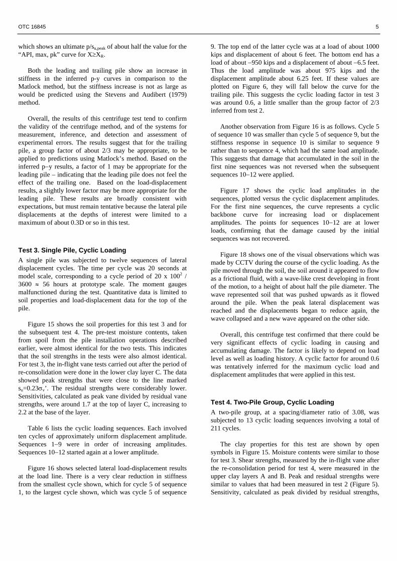
Figure 7 shows the bending moments measured in the pile. Also shown are curves obtained as polynomial least squares fits to the measured moments. The least-squares method used here is described in Appendix A. The method is probably not very accurate below about 130 feet below mudline, near the last of the bending moment transducers. The data show that, as expected, the maximum moment moves down the pile as the lateral load increases. The pile remained elastic up to about 95% of the maximum load. At this stage, first yield was reached in the pile, at a first yield moment My1 which was reached first at about 100 feet below mudline, and shortly after at about 75 feet below mudline. The bending moment transducers actually measure strains, so after this point the calibrations carried out under elastic conditions begin to become inaccurate.

Figure 8 shows the inferred lateral soil pressures. The method used to deduce these from the bending moments is described in Appendix A. Figure 8 also shows a curve marked “API, max, pk”. This corresponds to what would be calculated using Matlock’s method, with soil strengths inferred from the measured peak vane strengths for this test. For these calculations, ε50 was taken as 1.25%. The data show that relatively large pressures developed in the upper regions of soil initially. These then reduced as the load increased.

Figure 9 shows the inferred lateral pile displacements. The method used to deduce these from the bending moments is described in Appendix A. It involves double-integration of the polynomial fitted to the bending moment data. As noted in Appendix A, some small corrections were needed to ensure that the inferred lateral deflections at great depth were zero. The results are reasonably consistent with the deflections measured directly by the LVDTs near the tops of the piles (Figure 3).

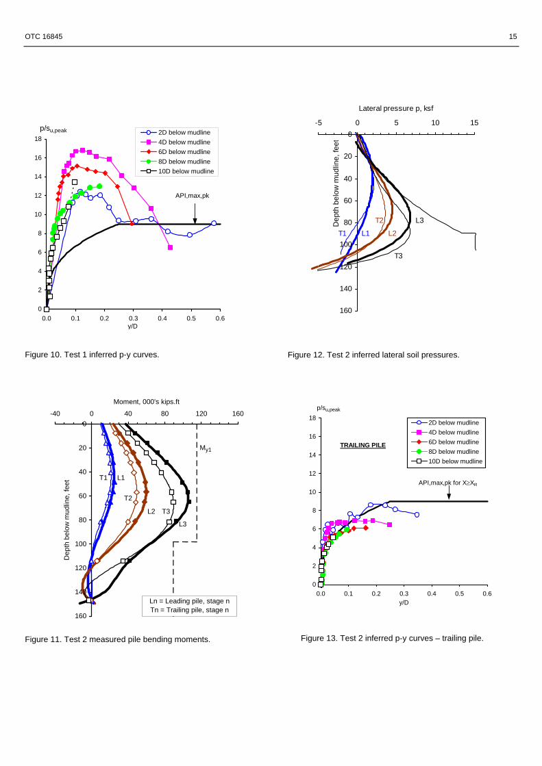
Figure 10 shows inferred p-y results based on the above calculations of lateral pressures and lateral deflections. The results are presented in normalized form; with lateral pressure divided by the undrained shear strengths based on the measured peak vane strengths and with deflection divided by pile diameter D. The last segments of each curve are shown dotted. These segments correspond to the transition from 95% to 100% of the maximum load, and the bending moment data are inaccurate in this segment as described above. Figure 10 also shows a curve “API, max, pk” corresponding to the Matlock curve for static loading with pu/su=9 at large deflections. The results show that the actual lateral resistances can be much larger than those predicted by Matlock at lower load levels. However, this may have been due to the under-

4 OTC 16845

consolidation of the clay in this test. For large deflections, the results indicate good agreement with the Matlock method. The inferred p-y curves also show a stiffer response then what would be calculated using Matlock’s method. The increased stiffness is consistent with the empirical formulation presented by Stevens and Audibert (1979), which would predict a 2.8 times increase in stiffness for the 100-inch pile diameter used in this test program.

Overall, the results of this first centrifuge test confirm the accuracy of the experimental systems. The Matlock method was found to correlate remarkably accurately with data at large displacements, though not at small ones. The results also produce the following puzzle. At the large deflections observed in the test, one would have expected the strains in the soil to be huge, from mudline to at least 60 feet below mudline. On this basis one would expect the residual soil strength to be relevant, not the peak strength. Care must therefore be exercised if it is desired to extrapolate results of these tests to soils with different sensitivities. Appendix B of this paper discusses the issue of sensitivity of ultimate lateral capacity to soil strength.

Test 2. Two-Pile Group, Static Loading A two-pile group, loaded in line at a spacing/diameter ratio of 3.08, was subjected to a static load test. The piles were connected by pinned links ensuring approximately equal cap displacements while allowing cap rotation (Figure 3). The time taken to load the piles, from zero to maximum lateral load, was around 100 seconds at model scale, corresponding to 100 x 1002 / (24 x 3600) ≈ 12 days at prototype scale.

The clay properties for this test are shown by open symbols in Figure 5. Moisture contents were noticeably different from the values for test 1. Shear strengths, measured by the in-flight vane after the re-consolidation period for test 2, were up to twice as large as in test 1. Peak strengths were larger than the line marked su=0.23σv’, which represents the expected critical state strengths at large strain. The residual strengths were close to this line, and lower. These different strength results indicate that the period of re-consolidation for this test 2 was sufficient to reduce the earlier under-consolidation, so that the clay was close to being fully re-consolidated during the pile load test.

Table 5 gives ultimate loads calculated on the basis of the measured strengths for this test, and assuming each pile to be unaffected by the presence of the other pile. The actual load-displacement results during the static test are shown in Figure 6. The test was not taken to complete failure. The results confirm a major difference between the leading and trailing piles, indicating that the piles did indeed affect each other. At the maximum lateral displacement of 6 feet, the load taken by the leading pile was about 12% greater than the load taken at the same displacement by the single pile in test 1. The load

taken by the trailing pile was about 12% less that the load for the single pile. The average of the two piles was about the same as for test 1.

These results may seem surprising at first, given that the soil strengths were about twice as large in test 2 compared to test 1. Appendix B of this paper develops a simplified analysis for ultimate capacity that shows that a two-fold change of soil strength would be expected to only produce an 18% change in ultimate pile load. On this basis, the load response in the leading pile in test 2 is 18-12=6% smaller than would have been the case if a single pile had been tested in soil of the same strengths as those that were measured in the two-pile Test 2. The load response of the trailing pile is 18+12 = 30% smaller.

Figure 11 shows the measured bending moments and the least-squares polynomial fits. Data are shown for the leading pile (L) and trailing pile (T), at stages 1, 2, and 3 of increasing applied load. The results for L3, leading pile at stage 3, suggest that a fault may have developed during stage 3 in the moment gauge that was 115 feet below mudline. Ignoring this result, the data confirm that the leading pile experienced larger bending moments.

Figure 12 shows the inferred lateral soil pressures. The rest for the lower part of L3 may have been unduly affected by the possible fault mentioned above. The results confirm that, for a considerable fraction of the contact depths, larger soil resistances were experienced at the leading pile.

Figure 13 shows the inferred normalized p-y curves for the trailing pile. Also shown is a curve marked “API, max, pk” which was computed using the measured soil strengths and Matlock’s method for a depth X greater that or equal to the depth XR of reduced resistance. The data suggest that the maximum lateral pressures on the trailing pile were significantly less than the Matlock prediction, with the curves perhaps tending to an ultimate resistance factor p/su,peak of about 6. Since the Matlock factor is 9, this gives a group factor of about 2/3 for the trailing pile. This value must remain tentative however as the lateral displacements reached only about 0.15D to 0.3D.

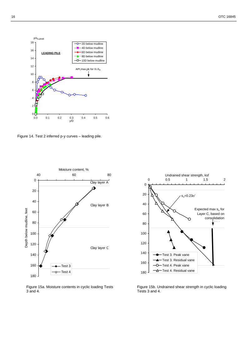
Figure 14 shows the inferred normalized p-y curves for the leading pile. Comparing the maximum displacements with those for the trailing pile, it is seen that larger displacements were inferred for the leading pile. This is thought to be due to a small error associated with the way the lateral displacements were inferred, see Appendix A. The error is not sufficient to invalidate the results. The results for depths of 4D and more below mudline show remarkable agreement with the Matlock method, suggesting a group factor of 1 for these depths and this pile in this soil. The depth of reduced resistance was calculated as just over four pile diameters (Table 5). Thus Matlock’s factor X/XR for 2D below mudline was about 1/2. This agrees very well indeed with the data for this depth,

OTC 16845 5

which shows an ultimate p/su,peak of about half the value for the “API, max, pk” curve for X≥XR.

Both the leading and trailing pile show an increase in stiffness in the inferred p-y curves in comparison to the Matlock method, but the stiffness increase is not as large as would be predicted using the Stevens and Audibert (1979) method.

Overall, the results of this centrifuge test tend to confirm the validity of the centrifuge method, and of the systems for measurement, inference, and detection and assessment of experimental errors. The results suggest that for the trailing pile, a group factor of about 2/3 may be appropriate, to be applied to predictions using Matlock’s method. Based on the inferred p−y results, a factor of 1 may be appropriate for the leading pile – indicating that the leading pile does not feel the effect of the trailing one. Based on the load-displacement results, a slightly lower factor may be more appropriate for the leading pile. These results are broadly consistent with expectations, but must remain tentative because the lateral pile displacements at the depths of interest were limited to a maximum of about 0.3D or so in this test.

Test 3. Single Pile, Cyclic Loading A single pile was subjected to twelve sequences of lateral displacement cycles. The time per cycle was 20 seconds at model scale, corresponding to a cycle period of 20 x 1002 / 3600 ≈ 56 hours at prototype scale. The moment gauges malfunctioned during the test. Quantitative data is limited to soil properties and load-displacement data for the top of the pile.

Figure 15 shows the soil properties for this test 3 and for the subsequent test 4. The pre-test moisture contents, taken from spoil from the pile installation operations described earlier, were almost identical for the two tests. This indicates that the soil strengths in the tests were also almost identical. For test 3, the in-flight vane tests carried out after the period of re-consolidation were done in the lower clay layer C. The data showed peak strengths that were close to the line marked su=0.23σv’. The residual strengths were considerably lower. Sensitivities, calculated as peak vane divided by residual vane strengths, were around 1.7 at the top of layer C, increasing to 2.2 at the base of the layer.

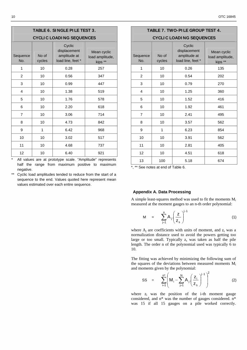
Table 6 lists the cyclic loading sequences. Each involved ten cycles of approximately uniform displacement amplitude. Sequences 1−9 were in order of increasing amplitudes. Sequences 10−12 started again at a lower amplitude.

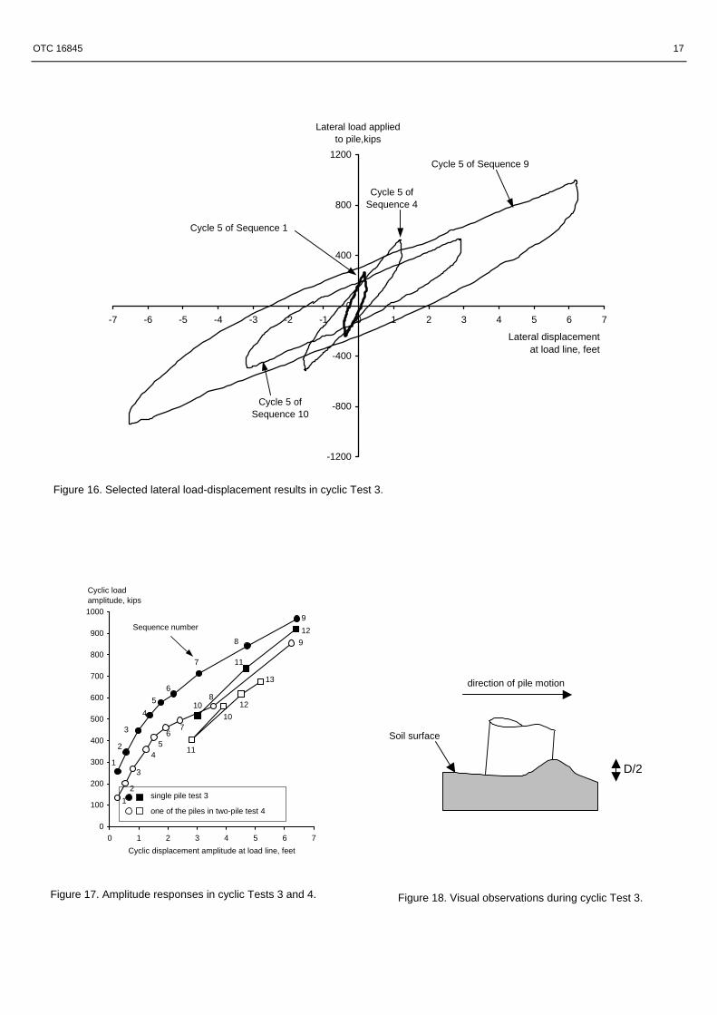
Figure 16 shows selected lateral load-displacement results at the load line. There is a very clear reduction in stiffness from the smallest cycle shown, which for cycle 5 of sequence 1, to the largest cycle shown, which was cycle 5 of sequence

9. The top end of the latter cycle was at a load of about 1000 kips and displacement of about 6 feet. The bottom end has a load of about −950 kips and a displacement of about −6.5 feet. Thus the load amplitude was about 975 kips and the displacement amplitude about 6.25 feet. If these values are plotted on Figure 6, they will fall below the curve for the trailing pile. This suggests the cyclic loading factor in test 3 was around 0.6, a little smaller than the group factor of 2/3 inferred from test 2.

Another observation from Figure 16 is as follows. Cycle 5 of sequence 10 was smaller than cycle 5 of sequence 9, but the stiffness response in sequence 10 is similar to sequence 9 rather than to sequence 4, which had the same load amplitude. This suggests that damage that accumulated in the soil in the first nine sequences was not reversed when the subsequent sequences 10−12 were applied.

Figure 17 shows the cyclic load amplitudes in the sequences, plotted versus the cyclic displacement amplitudes. For the first nine sequences, the curve represents a cyclic backbone curve for increasing load or displacement amplitudes. The points for sequences 10−12 are at lower loads, confirming that the damage caused by the initial sequences was not recovered.

Figure 18 shows one of the visual observations which was made by CCTV during the course of the cyclic loading. As the pile moved through the soil, the soil around it appeared to flow as a frictional fluid, with a wave-like crest developing in front of the motion, to a height of about half the pile diameter. The wave represented soil that was pushed upwards as it flowed around the pile. When the peak lateral displacement was reached and the displacements began to reduce again, the wave collapsed and a new wave appeared on the other side.

Overall, this centrifuge test confirmed that there could be very significant effects of cyclic loading in causing and accumulating damage. The factor is likely to depend on load level as well as loading history. A cyclic factor for around 0.6 was tentatively inferred for the maximum cyclic load and displacement amplitudes that were applied in this test.

Test 4. Two-Pile Group, Cyclic Loading A two-pile group, at a spacing/diameter ratio of 3.08, was subjected to 13 cyclic loading sequences involving a total of 211 cycles.

The clay properties for this test are shown by open symbols in Figure 15. Moisture contents were similar to those for test 3. Shear strengths, measured by the in-flight vane after the re-consolidation period for test 4, were measured in the upper clay layers A and B. Peak and residual strengths were similar to values that had been measured in test 2 (Figure 5). Sensitivity, calculated as peak divided by residual strengths,

6 OTC 16845

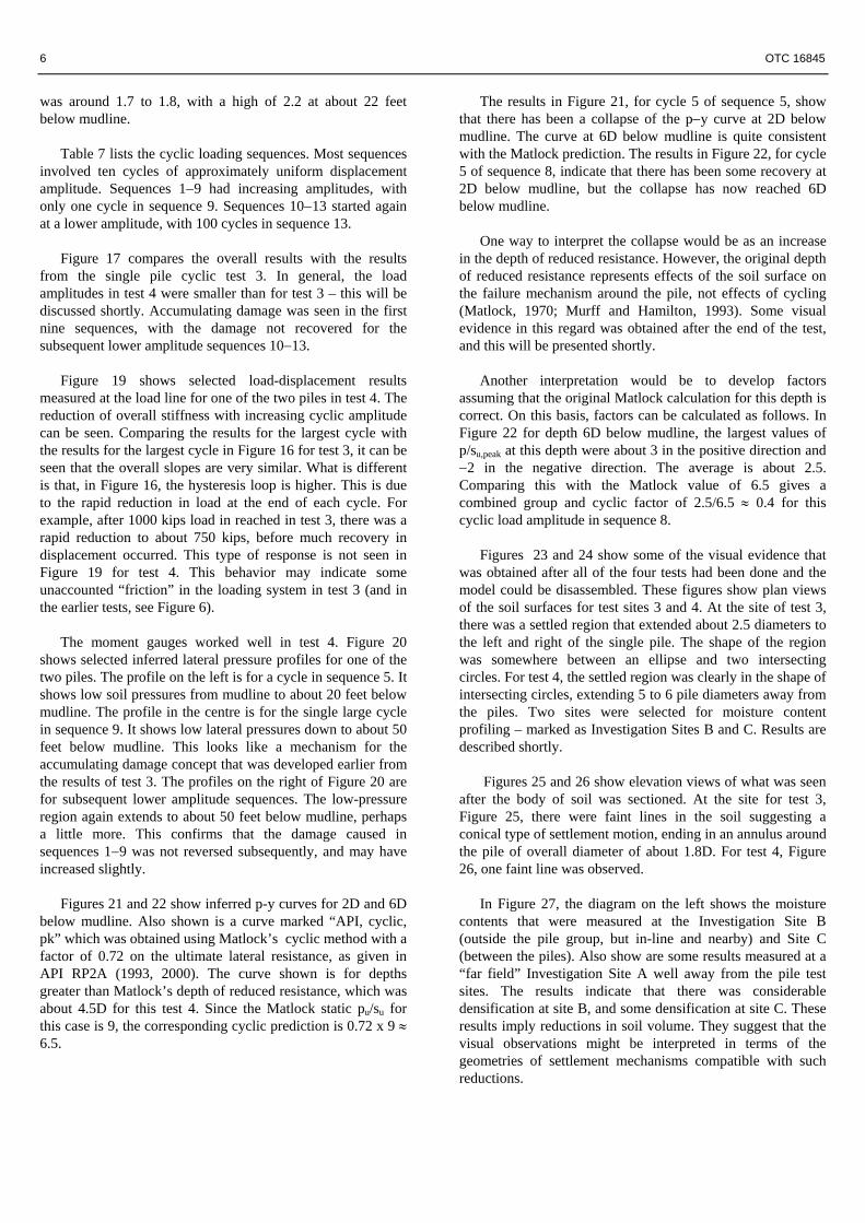
was around 1.7 to 1.8, with a high of 2.2 at about 22 feet below mudline.

Table 7 lists the cyclic loading sequences. Most sequences involved ten cycles of approximately uniform displacement amplitude. Sequences 1−9 had increasing amplitudes, with only one cycle in sequence 9. Sequences 10−13 started again at a lower amplitude, with 100 cycles in sequence 13.

Figure 17 compares the overall results with the results from the single pile cyclic test 3. In general, the load amplitudes in test 4 were smaller than for test 3 – this will be discussed shortly. Accumulating damage was seen in the first nine sequences, with the damage not recovered for the subsequent lower amplitude sequences 10−13.

Figure 19 shows selected load-displacement results measured at the load line for one of the two piles in test 4. The reduction of overall stiffness with increasing cyclic amplitude can be seen. Comparing the results for the largest cycle with the results for the largest cycle in Figure 16 for test 3, it can be seen that the overall slopes are very similar. What is different is that, in Figure 16, the hysteresis loop is higher. This is due to the rapid reduction in load at the end of each cycle. For example, after 1000 kips load in reached in test 3, there was a rapid reduction to about 750 kips, before much recovery in displacement occurred. This type of response is not seen in Figure 19 for test 4. This behavior may indicate some unaccounted “friction” in the loading system in test 3 (and in the earlier tests, see Figure 6).

The moment gauges worked well in test 4. Figure 20 shows selected inferred lateral pressure profiles for one of the two piles. The profile on the left is for a cycle in sequence 5. It shows low soil pressures from mudline to about 20 feet below mudline. The profile in the centre is for the single large cycle in sequence 9. It shows low lateral pressures down to about 50 feet below mudline. This looks like a mechanism for the accumulating damage concept that was developed earlier from the results of test 3. The profiles on the right of Figure 20 are for subsequent lower amplitude sequences. The low-pressure region again extends to about 50 feet below mudline, perhaps a little more. This confirms that the damage caused in sequences 1−9 was not reversed subsequently, and may have increased slightly.

Figures 21 and 22 show inferred p-y curves for 2D and 6D below mudline. Also shown is a curve marked “API, cyclic, pk” which was obtained using Matlock’s cyclic method with a factor of 0.72 on the ultimate lateral resistance, as given in API RP2A (1993, 2000). The curve shown is for depths greater than Matlock’s depth of reduced resistance, which was about 4.5D for this test 4. Since the Matlock static pu/su for this case is 9, the corresponding cyclic prediction is 0.72 x 9 ≈ 6.5.

The results in Figure 21, for cycle 5 of sequence 5, show that there has been a collapse of the p−y curve at 2D below mudline. The curve at 6D below mudline is quite consistent with the Matlock prediction. The results in Figure 22, for cycle 5 of sequence 8, indicate that there has been some recovery at 2D below mudline, but the collapse has now reached 6D below mudline.

One way to interpret the collapse would be as an increase in the depth of reduced resistance. However, the original depth of reduced resistance represents effects of the soil surface on the failure mechanism around the pile, not effects of cycling (Matlock, 1970; Murff and Hamilton, 1993). Some visual evidence in this regard was obtained after the end of the test, and this will be presented shortly.

Another interpretation would be to develop factors assuming that the original Matlock calculation for this depth is correct. On this basis, factors can be calculated as follows. In Figure 22 for depth 6D below mudline, the largest values of p/su,peak at this depth were about 3 in the positive direction and −2 in the negative direction. The average is about 2.5. Comparing this with the Matlock value of 6.5 gives a combined group and cyclic factor of 2.5/6.5 ≈ 0.4 for this cyclic load amplitude in sequence 8.

Figures 23 and 24 show some of the visual evidence that was obtained after all of the four tests had been done and the model could be disassembled. These figures show plan views of the soil surfaces for test sites 3 and 4. At the site of test 3, there was a settled region that extended about 2.5 diameters to the left and right of the single pile. The shape of the region was somewhere between an ellipse and two intersecting circles. For test 4, the settled region was clearly in the shape of intersecting circles, extending 5 to 6 pile diameters away from the piles. Two sites were selected for moisture content profiling – marked as Investigation Sites B and C. Results are described shortly.

Figures 25 and 26 show elevation views of what was seen after the body of soil was sectioned. At the site for test 3, Figure 25, there were faint lines in the soil suggesting a conical type of settlement motion, ending in an annulus around the pile of overall diameter of about 1.8D. For test 4, Figure 26, one faint line was observed.

In Figure 27, the diagram on the left shows the moisture contents that were measured at the Investigation Site B (outside the pile group, but in-line and nearby) and Site C (between the piles). Also show are some results measured at a “far field” Investigation Site A well away from the pile test sites. The results indicate that there was considerable densification at site B, and some densification at site C. These results imply reductions in soil volume. They suggest that the visual observations might be interpreted in terms of the geometries of settlement mechanisms compatible with such reductions.

OTC 16845 7

The diagram on the right of Figure 27 shows remolded shear strengths calculated from the moisture contents. The calculations assumed that remolded shear strength is 1.7 kPa at the liquid limit and 170 kPa at the plastic limit, varying exponentially for moisture contents between the limits (e.g., Wroth and Houslby, 1985; Powrie, 1997). Results were found to be sensitive to the value used for the plastic limit (Table 3). The relative values for one investigation site compared to another are probably fairly accurate. The results confirm that the largest increase in remolded strength occurred outside the pile group but near it. If the increased strengths occurred as a result of cyclic straining, then the results imply that there were less cyclic strains in the region between the piles. This observation sheds light on the nature of the likely strain field around and between the two piles.

Overall, the results of centrifuges tests 3 and 4 were consistent with each other and confirm that a mechanism of soil damage occurs during cyclic lateral loading. The damage increases with increasing cyclic amplitude, and is not reversed in subsequent lower amplitude cycles. The accumulation of damage may be important when considering platform lifetime, because it suggests that foundation response will change incrementally each time a storm or other loading event exceeds the severity of previous events.

Conclusions Results from the four centrifuge model tests provided useful and timely information for the foundation design of the URSA TLP.

The results of the tests confirmed the remarkable validity of Matlock’s method when applied to a single pile or to the leading pile of a two-pile group under static loading. For cyclic loading, a phenomenon of accumulating damage was identified, which is likely to be of interest in platform lifetime assessment. The test results confirmed significant group and cyclic loading effects for a two-pile group loaded in line at a centerline-to-centerline spacing/diameter ratio of 3.08. The following preliminary factors were obtained.

• For static loading, based on single pile test 1 and two-pile test 2, ratios were calculated of the ultimate lateral soil pressure on a pile in a two-pile group divided by the ultimate pressure on a single pile at the same displacement. The results were about 1 for the leading pile, indicating little effect of interaction, and 2/3 for the trailing pile. These factors would apply to Matlock’s static case.

• For cyclic loading of a single pile, based on tests 1 and 3, ratios were calculated for pressures during cyclic loading divided by corresponding pressures during static loading. The results depend on cyclic load amplitude. For one of the amplitudes investigated, a ratio of about 0.6 was inferred. This factor would apply to Matlock’s static case. It would

be equivalent to a factor of 0.6/0.72 ≈ 0.8 applied to his cyclic factor of 0.72.

• Based on all four tests, a combined group and cyclic factor of 0.4 was inferred for one of the cyclic load amplitudes. This is lower than the product of the group and cyclic factors combined (i.e., 2/3 x 0.8). Again this would apply in combination with Matlock’s cyclic case, giving an overall factor of 0.4 x 0.72 ≈ 0.29.

Design Implications Based on these very limited number of tests, several design implications could be inferred for laterally loaded piles with large deflections at an s/d of 3.08. They are:

1. The results of the tests confirmed the remarkable validity of Matlock’s method when applied to a single pile or to the leading pile of a two-pile group under static loading. Thus, large lateral displacements during static loading do not reduce Matlock’s ultimate lateral resistance factor.

2. For the static single pile test, stiffness increases due to large diameter affects were consistent with Stevens and Audibert (1979).

3. The group behavior in static loading shows that the leading pile is not affected by the trailing pile. While not discussed in this paper, the observed group behavior is consistent with several analytical methods. For example, the average of the sum of the lead pile group factor (i.e., one) and the trailing pile (i.e., 2/3) equals 0.84. This is consistent with several analytical methods to predict group behavior.

4. For single pile cyclic behavior, large lateral displacements reduce Matlock’s 0.72 factor by about 20% or to a factor of 0.60.

5. The soil surrounding the pile is remolded during cyclic loading.

6. A gap does not form between the pile and soil under cyclic loading conditions.

7. The lateral resistance factor during group cyclic loading is 0.29. Matlock has previously suggested that cyclic loading with large displacements will reduce the p-y curves. He suggested that the p-y curve not exceed 1/(soil sensitivity). For an approximate sensitivity of two for the Kaolin clay used in this study, the factor should have therefore been 0.5. The test result shows a factor considerably lower than that suggested by Matlock. Certainly, this result warrants further study.

8 OTC 16845

As a caveat to this design implication discussion, it must be remembered that these results are from a very limited number of tests and while well executed at a facility with considerable experience with centrifuge testing, more tests are warranted to better understand the lateral behavior of piles with large displacements.

Acknowledgement The Authors thank the operator of the Ursa field, Shell Exploration and Production Company, and its partners, BP, ExxonMobil and ConocoPhillips for permission to publish the data. We also thank the staff of Cambridge University’s Schofield Center for their efforts, which made these tests possible.

References

1. Airey, D.W. (1984), “Clays in simple shear apparatus”, Ph.D thesis, Cambridge University

2. Al-Tabbaa, A. (1984), “Anisotropy of clay”, M.Phil thesis, Cambridge University

3. Al-Tabbaa, A. (1987), “Permeability and stress-strain response of speswhite kaolin”, Ph.D thesis, Cambridge University

4. API (1993), “Recommended Practice for Planning, Designing and Constructing Fixed Offshore Platforms − Load and Resistance Factor Design”, RP2A-LRFD, American Petroleum Institute

5. API (2000), “Recommended Practice for Planning, Designing and Constructing Fixed Offshore Platforms − Working Stress Design”, RP2A-WSD, American Petroleum Institute

6. Clegg, D. (1981), “Model piles in stiff clay”, Ph.D thesis, Cambridge University.

7. Clukey, E.C., and Phillips, R. (2002), “Centrifuge Model Tests to Verify Suction Caisson Capacities for Taut and Semi-Taut Legged Mooring Systems), Proc Deep Offshore Technology Conf, New Orleans, paper available on http://dot2002.events.pennet.com/proceedings.htm

8. Craig, W.H. (1983), “Simulation of foundations for offshore structures using centrifuge modeling”, Developments in Soil Mechanics and Foundation Engineering – I, Model Studies, eds.P.K.Banerjee and R.Butterfield, Applied Science Publishers, Chapter 1, 1–27.

9. Craig, W.H., (ed) (1984), Application of Centrifuge Modeling Techniques to Geotechnical Design, Balkema

10. Craig, W.H., James, R.G., and Schofield, A.N., (eds) (1988), Centrifuges in Soil Mechanics, Balkema

11. Digre, K.A., Kipp, R.M., Hunt, R.J., Hanna, S.Y., Chan, J.H., Rosen, V., and van der Voort, C. (1999), “URSA TLP, tendon, foundation design, fabrication, transportation, and TLP Installation”, Paper OTC 10756, Offshore Technology Conf, Vol.2, Houston, May.

12. Elmes, D. (1986). “Creep and viscosity in two kaolin clays”, Ph.D thesis, Cambridge University

13. Fleming, W.G.K., Weltman, A.J., Randolph, M.F., and Elson,

W.K. (1992), Piling Engineering, 2nd edition, Blackie Academic & Professional

14. Garside, R., Bowen, K. G., Stevens, J. W., Doyle, E. H., Henry, D. M., and Romijn, E. (1997), “Mars TLP - integration and installation”, 29th Annual Offshore Technology Conference, OTC 8373, Houston, May.

15. Gatlin, M.E. (1999), “Operations role in the design and commissioning of the URSA TLP”, Paper OTC 10759, Offshore Technology Conf, Vol.2

16. Hamilton, J.M., Phillips, R., Dunnavant, T.W., and Murff, J.D. (1991), “Centrifuge study of laterally loaded piles in soft clay), Proc Int Conf Centrifuge 1991, ISSMFE

17. Hamilton, J.M., and Murff, J.D. (1995), “Ultimate lateral capacity of piles in clay”, Offshore Technology Conference, Paper OTC 7667, Vol.1, 241–255.

18. Matlock, H. (1970), “Correlations for design of laterally loaded piles in soft clay”, Paper OTC 1024, Offshore Technology Conf, 1, 577−594

19. Murff, J.D. (1996), “The geotechnical centrifuge in offshore engineering”, OTC 8265, Offshore Technology Conference, Vol.1, 675–689

20. Murff, J.D., and Hamilton, J.M. (1993), “P-ultimate for undrained analysis of laterally loaded piles”, ASCE Journal of Geotechnical Engineering, 119(1), 91−107

21. Powrie, W. (1997), Soil mechanics: concepts and applications. E & F N Spon, London

22. Schofield, A.N. (1980), “Cambridge geotechnical centrifuge operations”, Geotechnique, 30(3), 227–268

23. Springman, S.M. (1993), “Centrifuge modeling in clay marine applications”, Keynote Address, 4th Canadian Marine Geotechnical Conference, St.Johns, Newfoundland

24. Stevens, J. B. and Audibert, J. M. E. (1979), “Re-examination of p-y curve formulation”, Paper OTC 3402, Offshore Technology Conf, Vol.2, Houston, May.

25. Taylor, R.N., (ed) (1994), Geotechnical Centrifuge Technology, Blackie Academic & Scientific

26. Wroth, C.P., and Houlsby, G.T. (1985), “Soil mechanics − property characterization and analysis procedures”, Proc 11th ICSMFE, San Francisco, 1, 1−53

OTC 16845 9

TABLE 1. TEST CHARACTERISTICS Test 1 Test 2 Test 3 Test 4

Type Single pile Two-pile group* Single pile Two-pile

group*

Loading Static Static and cyclic Cyclic Cyclic

No of cyclic load sequences

− 2 12 13

Total number of cycles − 17 120 211

Observations Pile taken to failure

Some clay settlement

Extensive settlement

Extensive settlement

Height of load line above clay surface **

24′ 7′′ 26′ 3′′ 27′ 3′′ 27′ 3′′

Thickness of clay layer A ** 11′ 2′′ 10′ 10′′ 10′ 10′′ 10′ 10′′

Thickness of clay layer B ** 79′ 1′′ 78′ 5′′ 77′ 9′′ 77′ 9′′

Thickness of clay layer C ** 77′ 9′′ 77′ 1′′ 76′ 9′′ 76′ 9′′

* Prototype pile spacing (CL to CL) = 25′ 8′′ in tests 2 and 4, giving a spacing/diameter diameter ratio of 3.08.

** Dimensions at prototype scale.

TABLE 2. PROTOTYPE PILE CHARACTERISTICS Section Pile cap Upper Lower Plug

Length, feet 4’ 11’’ 117’ 9” 56’ 9” 13’ 2”

Outer diameter − 100” 100” 100/94”

EI, x 108 inch2.kips >300 210 163 >300

Equiv.wall thickness * − 1.95” 1.5” −

Moment at first yield, 000’s kips.ft **

− 115 89 −

Ultimate moment,000’s kips.ft **

− 291 223 −

* Equivalent wall thickness calculated on the basis of matching the prototype EI to a steel pile od of 100 inches.

** Moments at first yield and ultimate moments scaled from model values by multiplying by 1003.

TABLE 3. PROPERTIES OF SPESWHITE KAOLIN CLAY USED IN THE TESTS

Property Value(s) Data sources

Specific gravity Gs

2.61 − 2.64 Clegg (1981), Al-Tabbaa (1984, 1987), Elmes (1986)

Liquid limit 69 Airey (1984)

Plastic limit 38 Airey (1984)

su, normally consolidated 0.23 σ’v Clegg (1981)

TABLE 4. TEST 1. CALCULATED LATERAL CAPACITIES

Using peak soil strengths

Using residual soil strengths

Depth XR of reduced resistance

12 feet 6 feet

Lateral capacity, assuming limited by pile moment at first yield

1433 kips, first yield moment reached 79′

below mudline

1270 kips, first yield moment reached 90′

below mudline

Lateral capacity, assuming limited by ultimate pile moment

2470 kips, plastic hinge in pile 108′

below mudline

2190 kips, plastic hinge in pile 113′

below mudline

TABLE 5. TEST 2. CALCULATED LATERAL CAPACITIES

Using peak soil strengths

Using residual soil strengths

Depth XR of reduced resistance

36 feet 13 feet

Lateral capacity, assuming limited by pile moment at first yield

1620 kips, first yield moment reached 65′

below mudline

1540 kips, first yield moment reached 72′

below mudline

Lateral capacity, assuming limited by ultimate pile moment

2780 kips, plastic hinge in pile 85′ below mudline

2560 kips, plastic hinge in pile 95′ below mudline

10 OTC 16845

TABLE 6. SINGLE PILE TEST 3.

CYCLIC LOADING SEQUENCES

Sequence No.

No of cycles

Cyclic displacement amplitude at

load line, feet *

Mean cyclic load amplitude,

kips **

1 10 0.28 257

2 10 0.56 347

3 10 0.99 447

4 10 1.38 519

5 10 1.76 578

6 10 2.20 618

7 10 3.06 714

8 10 4.73 842

9 1 6.42 968

10 10 3.02 517

11 10 4.68 737

12 10 6.40 921

* All values are at prototype scale. “Amplitude” represents half the range from maximum positive to maximum negative.

** Cyclic load amplitudes tended to reduce from the start of a sequence to the end. Values quoted here represent mean values estimated over each entire sequence.

TABLE 7. TWO-PILE GROUP TEST 4.

CYCLIC LOADING SEQUENCES

Sequence No.

No of cycles

Cyclic displacement amplitude at

load line, feet *

Mean cyclic load amplitude,

kips **

1 10 0.26 135

2 10 0.54 202

3 10 0.79 270

4 10 1.25 360

5 10 1.52 416

6 10 1.92 461

7 10 2.41 495

8 10 3.57 562

9 1 6.23 854

10 10 3.91 562

11 10 2.81 405

12 10 4.51 618

13 100 5.18 674

*, ** See notes at end of Table 6.

Appendix A. Data Processing

A simple least-squares method was used to fit the moments Mi measured at the moment gauges to an n-th order polynomial:

M =

1jn

1j sj z

zA−

=∑ ⎟⎟

⎠

⎞⎜⎜⎝

⎛. (1)

where Aj are coefficients with units of moment, and zs was a normalization distance used to avoid the powers getting too large or too small. Typically zs was taken as half the pile length. The order n of the polynomial used was typically 6 to 10. The fitting was achieved by minimizing the following sum of the squares of the deviations between measured moments Mi and moments given by the polynomial:

SS = ∑ ∑=

−

=⎟⎟

⎠

⎞

⎜⎜

⎝

⎛⎟⎟⎠

⎞⎜⎜⎝

⎛−

*

.n

1i

21jN

1j s

iji z

zAM (2)

where zi was the position of the i-th moment gauge considered, and n* was the number of gauges considered. n* was 15 if all 15 gauges on a pile worked correctly.

OTC 16845 11

Differentiating SS with respect Ak and setting the result to zero gives:

∑=

n

1jjkj AB . = (3) ∑

=

n

1jiki MC .

with: Bkj = ∑=

−+−

⎟⎟⎠

⎞⎜⎜⎝

⎛* )()(n

1i

1j1k

s

i

zz

(4)

Cki =

)1k(

s

i

zz

−

⎟⎟⎠

⎞⎜⎜⎝

⎛ (5)

In the present tests, horizontal loads were applied at the pile tops, and the moments were zero at the load line. If z is taken as zero at this line, for the purposes of this calculation, then M=0 here implies A1=0. Applying the above equation 3 for k=2 to n then gives a further n-1 equations which allow the coefficients A2 to AN to be calculated for any given set of measured moments Mi. Figure 28 illustrates the equilibrium of a pile element between depths z and z+dz. In the present tests, the axial loads P were negligible. Taking moments about the centre of the element, and then using the above polynomial, gives:

Q = dzdM

=

2jn

1j sj

s zz1jA

z1

−

=∑ ⎟⎟

⎠

⎞⎜⎜⎝

⎛− )..( (6)

where Q is the shear force in the pile. Considering horizontal equilibrium, and again using the polynomial, gives:

p.D = dzdQ

− =

3jn

1j sj2

s zz2j1jA

z1

−

=∑ ⎟⎟

⎠

⎞⎜⎜⎝

⎛−−

− ).).(.( (7)

from which the net lateral soil pressure p is obtained. Provided the pile remains elastic and the axial loads P are negligible, the lateral deflections y obey:

EI. 2

2

dzyd

= M (8)

where EI is the pile flexural rigidity at coordinate z. Consider a pile section that starts at coordinate zo. Substituting for the moments M and integrating once gives:

dzdy

= odz

dy⎟⎠⎞

⎜⎝⎛

+ EIzs ∑

= ⎥⎥⎦

⎤

⎢⎢⎣

⎡⎟⎟⎠

⎞⎜⎜⎝

⎛−⎟⎟

⎠

⎞⎜⎜⎝

⎛n

1j

j

s

oj

s

j

zz

zz

jA

. (9)

where (dy/dz)o represents the deflected pile slope at the start of the section. Integrating again gives:

y = yo + (z−zo).odz

dy⎟⎠⎞

⎜⎝⎛

+ EIz2

s ∑=

n

1jj

j Rj

A. (10)

Rj =

j

s

o

s

o1j

s

1j

s zz

.z

zz

zz

zz

1j1

⎟⎟⎠

⎞⎜⎜⎝

⎛⎟⎟⎠

⎞⎜⎜⎝

⎛ −−

⎥⎥⎦

⎤

⎢⎢⎣

⎡⎟⎟⎠

⎞⎜⎜⎝

⎛−⎟⎟

⎠

⎞⎜⎜⎝

⎛+

++

(11)

where yo is the deflection at the start of the section. For the present calculations, two methods were explored for finding (dy/dz)o and yo: (1) Starting from the measured slopes and deflections at the

top of the pile, use the equations for each section to compute the values for the top of the next section, or

(2) Starting from the bottom of the pile, and assuming dy/dz and y should be zero there, work upwards back-calculating the (dy./dz)o and zo values at the start of each section such that they give the inferred values of (dy/dz) and z at the base of the section.

It was found that the first method gave slopes dy/dz at the base of the pile that were small but non-zero. This was likely due to small inaccuracies in the measurement of the rotation of the top of the pile. Consequently, the second method was used for calculating dy/dz. Once the slopes (dy/dz)o were so obtained, the deflections calculated using the first method gave close to zero deflection at the base of the pile. Final estimates of deflections were then obtained using the second method. Appendix B. Simplified Ultimate Lateral Capacity Calculation

Calculations indicated that lateral pile capacity was rather insensitive to soil strengths for the present tests. One way to explore this is as follows. Figure 29 shows a pile loaded laterally by a force F acting at a height H above the mudline. Suppose the undrained soil strength at depth z below mudline is kz, and that the ultimate lateral soil resistance of pu=n.kz is mobilized. If the zone of reduced resistance is ignored then n is 9 for static loading, or 9 x 0.72 for cyclic loading, based on API (1993, 2000). Suppose the pile is sufficiently long that failure occurs by the formation of a plastic hinge at some depth zhinge below mudline. Let the hinge moment be Mp. Taking moments about the hinge gives:

F.(H+zhinge) = Mp + 6

1n.k .D (12) 3

hingez

A minimum force F=Fult is obtained by differentiating and setting the result to zero. This gives:

4p

D.k.n

M = ⎟⎟

⎠

⎞⎜⎜⎝

⎛+⎟⎟

⎠

⎞⎜⎜⎝

⎛

3D/z

2D/H.

Dz hinge

2hinge

(13)

The quantity on the left represents the pile strength Mp divided by a quantity depending on the soil strength. Denoting this quantity by ψ, and putting the result into equation 12 gives:

12 OTC 16845

p

ult

MD.F

= )D/z()D/H(

)6/(11

hinge+ψ+

(14)

For the particular case of loading at the mudline, H=0, and the equation reduces to:

Fult = 3

2p nkD.M3 .

21

(15)

Hence in this case the ultimate load depends only on the 1/3 power of the soil strength. For the present pile, we might take Mp as the first yield moment of 115000 kips-ft (Table 2). The rate of increase of soil strength with depth can be estimated from Figures 5 or 15. A representative value could be around k=1/100 ksf/foot. For static loading, n=9. The prototype pile diameter D was 100”. The above equations then give: • For the full soil strength of k=1/100 ksf/foot and taking

H/D=3, gives ψ=265, zhinge/D=8, and Fult.D/Mp = 0.091 • For half this strength, i.e. k=1/200 ksf/foot, and again with

H/D=3, gives ψ=530, zhinge/D=10.4, and Fult.D/Mp=0.075 Thus a reduction of shear strength by a factor of 2 would only reduce the ultimate capacity by (0.091−0.075)/0.091 = 18% in this simplified case. This confirms that, for the present tests, the ultimate lateral pile capacities were rather insensitive to soil strengths. Figure 1. General arrangement of tests – elevation

F

CLAY

Fd

Pile Test 1

Pile Test 2Pile Test 3

Pile Test 4

850mm diameter tubCLAY

igure 2. Plan view of pile and vane test sites.

igure 3. Pile lateral loading arrangement and lateral isplacement transducers.

OTC 16845 13

Figure 4. Instrumented model pile dimensions given at prototype scale.

Figure 5a. Soil properties in static loading Tests 1 and 2.

0

20

40

60

80

100

120

140

160

180

40 60 80 100Moisture content, %

Dep

th b

elow

mud

line,

feet

Test 1

Test 2

Clay layer A

Clay layer B

Clay layer C

M1

M9

M10

M12

M8

M2

M3

M11

M4

M5

M6

M7

M14

M15

M13

Venting tube

Connector to links of loading system

Load line

Clay Layer C

Clay Layer B

Clay Layer A

Mudline

4.9'P

ile S

ectio

n 1.

Len

gth

117.

8 fe

etP

ile S

ectio

n 2.

Len

gth

56.8

feet

Plug

Firm base

Pile, od 100"

Figure 5b. Soil properties in static loading Tests 1 and 2.

0

20

40

60

80

100

120

140

160

180

0 0.5 1 1.5Undrained shear strength su, ksf

2

Test 1. Peak vaneTest 1. Residual vaneTest 2. Peak vaneTest 2. Residual vane

su=0.23σ'

Expected su for Layer C, based

on consolidation

14 OTC 16845

-800

-400

0

400

800

1200

1600

0 2 4 6 8 10 12Lateral displacement at load line, feet

Late

ral l

oad

on p

ile, k

ips

Test 2. Leading Pile

Test 2. Trailing Pile

Test 1. Single Pile

14

Figure 6. Lateral load-displacement results in static loading Tests 1 and 2. Figure 7. Test 1 measured pile bending moments.

Fig

0

20

40

60

80

100

120

140

160

-40 0 40 80 120 160

Moment, 000's kips.ft

Dep

th b

elow

mud

line,

feet

At 40% of max loadAt 60% of max loadAt 80% of max loadAt 95% of max loadAt max load

Fig

ure 8. Test 1 inferred lateral soil pressures.

0

20

40

60

80

100

120

140

160

-5 0 5 10 15

Lateral pressure p, ksf

Dep

th b

elow

mud

line,

feet

60%

40%

80% 95%

100%

API,max,pk

0

20

40

60

80

100

120

140

-1 0 1 2 3 4 5

Lateral deflection y, feet

Dep

th b

elow

mud

line,

feet

40%

95%

60%

80%

100%

ure 9. Test 1 inferred lateral pile displacements.

OTC 16845 15

Figure 10. Test 1 inferred p-y curves. Figure 11. Test 2 measured pile bending moments.

0

20

40

60

80

100

120

140

160

-5 0 5 10 15

Lateral pressure p, ksf

Dep

th b

elow

mud

line,

feet

T1

0

2

4

6

8

10

12

14

16

18

0.0 0.1 0.2 0.3 0.4 0.5 0.6y/D

p/su,peak 2D below mudline4D below mudline6D below mudline8D below mudline10D below mudline

API,max,pk

T2

L2

T3

L1

L3

Figure 12. Test 2 inferred lateral soil pressures.

0

20

40

60

80

100

120

140

160

-40 0 40 80 120 160

Moment, 000's kips.ft

Dep

th b

elow

mud

line,

feet

Ln = Leading pile, stage nTn = Trailing pile, stage n

T1

T2

T3

L1

L2

L3

My1

0

2

4

6

8

10

12

14

16

18

0.0 0.1 0.2 0.3 0.4 0.5 0.6y/D

p/su,peak

2D below mudline4D below mudline6D below mudline8D below mudline10D below mudline

API,max,pk for X≥XR

TRAILING PILE

Figure 13. Test 2 inferred p-y curves – trailing pile.

16 OTC 16845

Figure 14. Test 2 inferred p-y curves – leading pile.

0

2

4

6

8

10

12

14

16

18

0.0 0.1 0.2 0.3 0.4 0.5 0.6y/D

p/su,peak

2D below mudline4D below mudline6D below mudline8D below mudline10D below mudline

API,max,pk for X≥XR

LEADING PILE

Figure 15a. Moisture contents in cyclic loading Tests 3 and 4.

0

20

40

60

80

100

120

140

160

180

40 60 80Moisture content, %

Dep

th b

elow

mud

line,

feet

Test 3

Test 4

Clay layer A

Clay layer B

Clay layer C

0

20

40

60

80

100

120

140

160

180

0 0.5 1 1.5Undrained shear strength, ksf

2

Test 3. Peak vaneTest 3. Residual vaneTest 4. Peak vaneTest 4. Residual vane

su=0.23σ'

Expected max su for Layer C, based on

consolidation hi t

Figure 15b. Undrained shear strength in cyclic loading Tests 3 and 4.

OTC 16845 17

Figure 17. Amplitude responses in cyclic Tests 3 and 4.

-1200

-800

-400

0

400

800

1200

-7 -6 -5 -4 -3 -2 -1 0 1 2 3 4 5 6 7

Lateral displacement at load line, feet

Cycle 5 of Sequence 9

Cycle 5 of Sequence 4

Cycle 5 of Sequence 10

Cycle 5 of Sequence 1

Lateral load applied to pile,kips

Figure 16. Selected lateral load-displacement results in cyclic Test 3.

0

100

200

300

400

500

600

700

800

900

1000

0 1 2 3 4 5 6 7Cyclic displacement amplitude at load line, feet

1

6

3

2

45

7

8

9

10

11

12Sequence number

1

6

4

3

2

5

7

8

9

10

11

12

13

Cyclic load amplitude, kips

one of the piles in two-pile test 4

single pile test 3

direction of pile motion

D/2

Soil surface

Figure 18. Visual observations during cyclic Test 3.

18 OTC 16845

Fi

Fi

-1200

-800

-400

0

400

800

1200

-7 -6 -5 -4 -3 -2 -1 0 1 2 3 4 5 6

Displacement at load line, fe

Sequence 9

Sequence 5

Lateral load applied to pile, kips

gure 19. Selected lateral load-displacement results in cyclic loading Test 4.

0

20

40

60

80

100

120

140

160

-12 -6 0 6 12

Lateral pressure at max pile load, ksf

Depth below mudline, feet

0

20

40

60

80

100

120

140

160

-12 -6 0 6 12

Lateral pressure at max pile load, ksf

0

20

40

60

80

100

120

140

160

-12 -6 0 6 12

Lateral pressure at max pile load, ksf

10

13

Depth below mudline, feetDepth below mudline, feet

gure 20. Selected lateral pressure profiles from cyclic loading Test 4.

OTC 16845 19

Figure 21. Inferred p-y curves Test 4, Cycle 5 of Sequence 5. Figure 22. Inferred p-y curves Test 4, Cycle 5 of Sequence 8.

-9

-6

-3

0

3

6

9

-0.15 -0.10 -0.05 0.00 0.05 0.10 0.15Y/D

2D below mudline

6D below mudlineAPI,cyclic,pk

p/su,peak

-

Fc

-9

-6

-3

0

3

6

9

-0.3 -0.2 -0.1 0.0 0.1 0.2 0.3Y/D

2D below mudline

6D below mudline API,cyclic,pk

p/su,peak Ff

~ 2.5 D ~ 2.5 D

Pile hole, diameter D

approximate edge of settled area

Directions of pile displacements during test

igure 23. Plan view of settled area around single pile for yclic Test 3.

Pile hole, diameter D

Pile hole, diameter D

~ 6 D ~ 5 D

approximate edge of settled area

Investigation site B

Investigation site C

Directions of pile displacements during test

igure 24. Plan view of settled area around two-pile group or cyclic Test 4.

20 OTC 16845

Figure 25. Elevation view of soil after sectioning single pile cyclic Test 3. Figure 27a. Moisture Contents near the two-pile group after cyclic Test 4.

~ 1.8D ~ 1.8D

~D/2

~3D

~ 1.8D

D

soil surface

faint linefaint line

~

~4D

~1.3D

~D/3

faint line

soil surface

Figure 26. Elevation view of soil after sectioning two-pile group cyclic Test 4.

0

20

40

60

80

100

120

140

160

180

20 40 60 80 100Moisture content, %

Dep

th b

elow

mud

line,

feet

Investigation Site AInvestigation Site BInvestigation Site C

0

20

40

60

80

100

120

140

160

180

0.0 1.0 2.0 3.0

Inferred remoulded shear strength, ksf

Dep

th b

elow

mud

line,

feet

Investigation Site A

Investigation Site B

Investigation Site C

Figure 27b. Rmoulded shear strengths near the two-pile group after cyclic Test 4.

OTC 16845 21

Figure 28. Forces on a pile segment.

dz

y

z

P

P+dP

p.D.dz

Q

Q+dQ

M

M+dM

segment of pile of

diameter D

H

zhinge

F

Mp

Lateral soil resistance = pu.D per unit length,

with pu = n.su and su=kz.

Hinge

Figure 29. Simplified calculation for ultimate lateral capacity of a long pile in normally consolidated soil.