osi ofs2000 cheat sheet for pml - pmlprocess.com … · ofs2000 cheat sheet for training course...
TRANSCRIPT
1
OFS2000 Cheat Sheet for Training Course
(Revision 3) By Paul Lawrence, PML Process Technology
Necessary Handouts include: Manual, RATA pages, Service Menu, and DSP settings page.
Models available: 2000, 2000F, 2000P, 2000W, 2000V Commissioning Concerns: •Optical Path Obstruction: Cables in Receiver box, Duct Braces / Baffles, Reflections/shinning surfaces, ambient light •Vibration: Scintillation frequency is 30Hz to 1000Hz, vibration outside this is o.k. •Electrical Concerns: Needs good ground, Run signal cable separate from power lines and transformers •Correction factor for angled ports is 1.41 for 45 degrees. (1 over the Cos of theta). •Keep heads cool (well below 140 degrees F) •Heater sometimes needed for cold air applications, use air heater upstream. •Weep hole in spool piece, needed in high moisture applications. Plug up or use, as needed. Start-up: Orient detector board with flow, Check that purge nozzles are oriented 90 degrees to flow to be measured, Set up purge (passive or active), Check diagnostic LEDS’s (9), Use bright flashlight and look in the pipe stubs, check that windows are clean and heater tabs hot. •Aim LED Adjust brightness to maximum using coarse and fine pots first, Adjust aim just by looking at red reflection, Can do fine adjust with remote DVM using C1 (A) and C2 (B) signals, try and get A & B voltages within 30% of each other. •Make sure doors are shut •Replace bolts as necessary Faults and Problems: •Log A & B voltages monthly (along with correlation number), to establish rate of decrease. Clean window display comes on when signal is < 0.5 for 5 minutes or more. •Fault relay changes state on: A&B signals out of range (light), Fails calibration, Power off, fails self test. (Note: Fault Relay is energized to open when no fault exists – opposite of what most people want – they can change this on order. Usually closed when no fault is the failsafe condition). •4-20 drives to 0ma on a fault (or 4ma as determined by set-up) •Calibration relay changes state when in calibration •Red LED on I/O board indicates open 4-20mA •Log correlation number, A&B and Velocity monthly to check trends in response. Calibration: •It has an external trigger or can be timed internally, 24 hour internal timing is typical and a manual calibration starts the cycle., External calibration is the RATA, can adjust readings with a correction factor and this can be linear or non-linear (six point). Steps for a RATA: (1) Do visual inspection and check that temp and pressure values are not way off between plant and RATA team. (2) Do two reference method runs at each load , if
Pg 1

2
they are within 5% of each other then o.k.. (3) Calculate the curve fit from these pre-RATA numbers and put it in the OFS (4) Proceed with the RATA. (Remember, if fuel source changes, velocity will be different to maintain the same load). Special Trouble shooting: •Can record RS232 data, (some companies use a PLC to convert RS232 to Modbus). Can record raw analog signals of A & B using stereo VCR audio channels. (Use CHA & CHB and shield as Pwr Rtn, Use Line-in input jacks on VCR – must record in stereo). Hands ON: •Play with: Normal Menu, Secret service Menu, Aiming LED, RS232 recording and curve fitting using laptop, LED change, DVM of A & B intensity, VCR recording, receiver board replacement, LED’s in heads and controller. Theory: •Theory of operation and DSP chip changing. •Lift off correlation is 30 at higher flow values. (It is higher at lower flow values). •Bi-directional capability only with chip 51”G”, 51 “F” is uni-directional. Bi-directional information is only on the RS232 output. •LED is gated and an AC signal. Detectors use synchronous detection method. • Why readings may not be exact and factors involved: -Velocity profile may not be uniform -Velocity profile may shift (in extreme cases, low flow in large stacks can ‘snake’) -OFS doesn’t have exactly the same sensitivity at all points along the pathlength. -OFS is not equally sensitive to gases of low temperature compared to gases of higher temperature. (low temperature gases have weak scintillation signal – if there is an influx of cold air into hotter air and not enough time for it to mix and homogenize, the OFS will preferentially “see” the hot). -Direction of flow can cause error and lower correlation (can get cross flow component). -Correction factor / linearization / curve fit. -Sample & Hold (S&H) Algorithm: There is a s& h and it is used to protect against a transitory loss of correlation. This is especially seen when the instrument is starting up and shutting down. The correlation parameter is such a fundamentally important one for operation of the meter that it has to be very carefully watched by the meter. The s & h is triggered when the rate of change of the correlation is very high. If the correlation is lost the instrument goes through a set of routines to find it again. The s&h is triggered during this process until the correlation is found. Sometimes it finds it faster than at other times. The duration of the s&h is dependant on the TC and lasts longer at high TC values.
Pg 2
General Guide to Initial OFS 2000 Flow Sensor Setup
Optical Scientific, Inc 2 Metropolitan Court Suite 6 Gaithersburg, MD 20878 Tel: 301 963 3630 Fax: 301 948 4674 www.opticalscientific.com
1
The Optical Scientific OFS (Optical Flow Sensor) 2000. Is the most reliable and accurate instrument available on the market for measuring air flow through a smoke stack, air duct, exhaust port, wind tunnel, or similar application. However. for it to perform with top efficiency, proper alignment of the Transmitter and Receiver is critical. This guide will show how to install your unit for maximum efficiency. This procedure and/or portions thereof are not dependent on operational status of the site. Some sections are of course easier if performed when operations are off-line, but customer processes need not be interrupted. Since OFS is designed with several options, and applications can vary due to the requirements, installation details illustrated may not match your particular setup. The procedures shown are common to all.
Note: this guide is a supplement to the OFS 2000 User's Guide shipped with your unit. If you have questions not covered here - refer to the User's Guide.
If you still have a question, call OSI Tech Support 301 963 3630 xt 216.
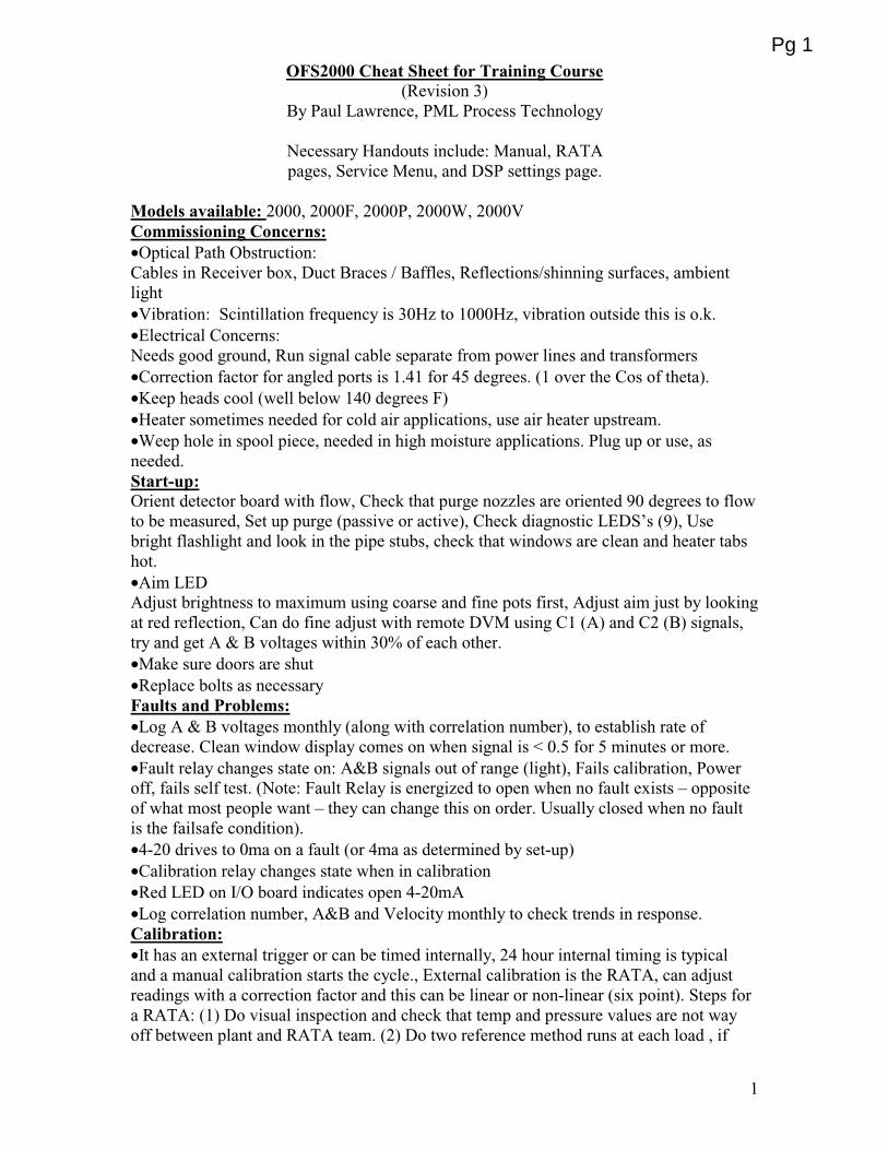
Flange Installation If your installation has flanges already installed, you may skip this section. The OFS Transmitter and Receiver are designed to mount to standard 4" pipe flanges mounted in the sides of the smokestack, duct, or plenum to be monitored. Placement and proper alignment of these pipe flanges is very important. If flanges are to be installed, they should be placed diametrically opposite one another, on the same horizontal plane. The center line of each pipe should be aligned as closely on the same axis as possible. When the flanges have been installed, you can proceed to install the OFS Sensor heads. [Refer to Installation Considerations in the OFS 2000 User's Guide p. 9]
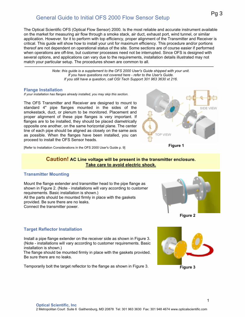
Caution! AC Line voltage will be present in the transmitter enclosure. Take care to avoid electric shock.
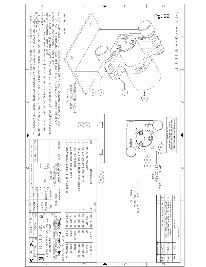
Transmitter Mounting Mount the flange extender and transmitter head to the pipe flange as shown in Figure 2. (Note - installations will vary according to customer requirements. Basic installation is shown.) All the parts should be mounted firmly in place with the gaskets provided. Be sure there are no leaks. Connect the transmitter power.
Figure 2
Target Reflector Installation Install a pipe flange extender on the receiver side as shown in Figure 3. (Note - installations will vary according to customer requirements. Basic installation is shown.) The flange should be mounted firmly in place with the gaskets provided. Be sure there are no leaks. Temporarily bolt the target reflector to the flange as shown in Figure 3.
Figure 3
Figure 1
Pg 3

General Guide to Initial OFS 2000 Flow Sensor Setup
Optical Scientific, Inc 2 Metropolitan Court Suite 6 Gaithersburg, MD 20878 Tel: 301 963 3630 Fax: 301 948 4674 www.opticalscientific.com
2
Figure 4
Figure 5
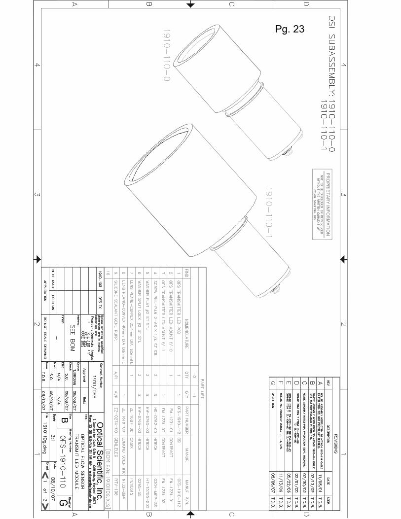
Transmitter Setup Turn the Transmitter power ON. Open the transmitter rear door. See that the power and signal LEDs are lit. Set the power output rotary switch to "1" (maximum output). Look through the transmitter window to the receiver aperture on the other side. You should see a bright reflection from the target reflector. Although care is taken in the initial installation of the mounting flanges, the beam may not be properly centered. Note: You will have to peer through the transmitter window to determine where the light beam is striking on the receiver side. Daylight or ambient light may make this difficult to see. You can use a dark cloth or jacket to block this light from entering your vision much like the old fashioned photographers. Patience in this part of the procedure will be well rewarded. Turn the transmitter module adjustment screws as directed in the User's Guide until the beam reflection is centered. The upper knob adjusts the transmitter module up and down, the lower knob adjusts the beam side-to-side. Adjust the transmitter module until the beam is centered on the receiver opening as shown. Remove the OFS Target Reflector and install the OFS Receiver in it's place. Again, use the gaskets supplied and be sure that the unit is mounted securely so that there are no air leaks. Receiver Setup Connect the receiver to the control unit and start the system. Watch the control panel display. Let the system run through it's start-up sequence and give it a few minutes to settle down. Note: data will not be judged as valid until the unit is properly aligned. Open the receiver unit and check the power and signal LEDs to make sure you have power and the unit is receiving a signal. See that the arrow on the back of the receiver PCB is pointing in the direction of flow. See Figure 6
Final Alignment Observe the A and B voltage readings on the control panel display. Adjust the transmitter module adjustment screws until the maximum A & B voltage values are displayed. A & B voltage range is from 1V to 9V. If voltage is near top of the scale (approaching saturation) adjust the transmitter power switch SW1 to bring the reading down into mid-range (1 = max power 4 = min. power.) See Figures 7 and 8. During operation it is normal for A & B voltage to fluctuate. Also, the voltages need not match exactly. The signal strength is influenced slightly by movement of air between the transmit and receive heads. Allow the unit to stabilize after each adjustment and repeat if necessary. Once the voltages have found their upper and lower limits, the alignment is considered to be compete.
Figure 7
Figure 8
light beam
Figure 6
Pg 4
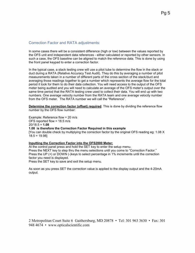
Correction Factor and RATA adjustments: In some cases there will be a consistent difference (high or low) between the values reported by the OFS unit and independent data references - either calculated or reported by other sensors. In such a case, the OFS baseline can be aligned to match the reference data. This is done by using the front panel keypad to enter a correction factor. In the typical case, a stack testing crew will use a pitot tube to determine the flow in the stack or duct during a RATA (Relative Accuracy Test Audit). They do this by averaging a number of pitot measurements taken in a number of different parts of the cross section of the stack/duct and averaging those readings together to get a number which represents the average flow for the total period it took for them to do their data collection. You will need access to the output of the OFS meter being audited and you will need to calculate an average of the OFS meter’s output over the same time period that the RATA testing crew used to collect their data. You will end up with two numbers. One average velocity number from the RATA team and one average velocity number from the OFS meter. The RATA number we will call the “Reference”. Determine the correction factor (offset) required. This is done by dividing the reference flow number by the OFS flow number: Example: Reference flow = 20 m/s OFS reported flow = 18.5 m/s 20/18.5 = 1.08 1.08 is therefore the Correction Factor Required in this example [You can double check by multiplying the correction factor by the original OFS reading eg: 1.08 X 18.5 = 19.98] Inputting the Correction Factor into the OFS2000 Meter: At the control panel press and hold the SET key to enter the setup menu. Press the NEXT key to step thru the menu selections until you come to “Correction Factor.” Press the UP (+) or DOWN (-)keys to select percentage in 1% increments until the correction factor you need is displayed. Press the SET key to save and exit the setup menu. As soon as you press SET the correction value is applied to the display output and the 4-20mA output. 2 Metropolitan Court Suite 6 Gaithersburg, MD 20878 • Tel: 301 963 3630 • Fax: 301 948 4674 • www.opticalscientific.com
Pg 5

3
MultiPoint Offset Procedure To perform multipoint offset to adjust the OFS measurement to the reference, one has to use computer to input the data to OFS. The front panel on OFS can only show inputted multipoint offset data but can’t perform any change. This is to protect the data from being altered arbitrarily by unauthorized personnel. Connect the OFS to a PC with the RS-232 connection procedure in next section. On PC, launch OSI’s program “QwikCollect”. Any other communication program should do, but here we only show the procedure using QwikCollect. On the main menu, click on File then on Terminal. Click OK on terminal prompt to get into Terminal Mode. Once in Terminal mode, the screen will be divided in two. The upper window contains a header Send and the lower window contains a header Receive. Go to top menu CommPort and click on comm1 or comm2 and set the Baud rate the same as OFS (OFS default is set at 9600 Baud rate). Click anywhere in the top window so the top window is active, Type “X” (upper case) in the top window. The bottom window shows the message “Enter the number of data point 0 to 6. Enter 0 to disable the curve fitting function. Press <esc> will abort the number entry mode.” Enter the number of data points for offsetting (e.g., 3 for low, mid, and high loads offsetting), then press <ret> key. Note: If you want to reset the offsetting values such as erase the previous multipoint offsetting data, type 0 and <ret>. The bottom screen shows “sending data to DSP” then shows a sequence like “D, 0, 1, 2, 10, --, 60, F, 100, G, 500, X, 0, 0”. If you see the last two comma divided items are 0, then the multipoint offset is reset. On the bottom window, the program will ask for unit of measure. Enter a number between 0 and 4 for the unit of measure and press <ret> key. The bottom window will ask for the input OFS speed #1, type in the OFS speed #1 in the top window. The bottom window will follow by asking input Reference speed #1. Please note the DSP can accept input of 1 to 4 digits, or 1 to 2 digits plus decimal point plus one digit after decimal point. For example, if you enter 15.42, the DSP will give you error message unless you type in 15.4. Continues inputting OFS #2 followed by Reference #2 until all the data pairs are entered. It should be noted the data pairs #1, #2, ... have to be entered in sequence from low value to high value. Upon pressing send after the last data point, OFS will show “Sending Data to DSP”. Wait for a few seconds, the program will show confirmation message in the form of “D, 0, 1, 2, 10, --, 60, F, 100, G, 500, X, 3, 0, 0005, 0006, 0010,, 0009, 0015, 0016”. In this example, the last eight comma divided items shows there are 3 pairs entry with unit of measure m/s (represented by 0). The first pair shows OFS speed entered is 5 m/s, and the reference speed entered is 6 m/s (low load). The second pair shows the OFS speed entered is 10 m/s and the reference speed entered is 9 m/s (mid load). The third pair shows the OFS speed entered is 15 m/s and the reference speed entered is 16 m/s (high load). To verify the data entered that are actually saved in the DSP, follow “Show Curve Fitting Values” procedure below. For details, refer to section “Set-up using OFS Keypad & Display” in the user’s manual. Show Curve Fitting Value Press �
Press � key to show current OFS and Ref values up to 6 points. Press NEXT to advance to the next display.
Curve Fitting Units
Default is Meter per Second. Press � or � keys to select a new unit of measure. Press NEXT to advance to the next display.
Curve Fitting Values OFS1=xx.x Ref1=yy.y
The final curve fitting values are displayed line by line. Press NEXT to show the next pair values until all points are displayed.
NOTE: Allcommandsare typedasCAPITALS
NOTE:Enter datainascendingorder
Erasing anold curve-fit
Pg 6

4
RS-232 Connections The OFS Interface Board has an RS-232 socket J2, a female DB25 connector, which is configured as a DCE device and has the following pin designation
Pin 2: RX Pin 3: TX Pins 1 and 7: Return
For a typical Personal Computer, the serial port is through a DB-25 male connector that is treated as a DTE device with the following pin designation
Pin 2: TX Pin 3: RX Pin 7: Return
A DB-25 male (OFS side) to DB-25 female (PC side) cable should provide adequate communication link because it has pin-to-pin straight connection. For a typical Laptop computer, the serial port is through a DB-9 male connector that has following configuration
Pin 2: RX Pin 3: TX Pin 5: Return
A DB-25 male (OFS side) to DB-9 female (PC side) cable should provide adequate communication link because it has a crossover between Pins 2 and 3, and pin 5 of DB-9 is connected to pin 7 of DB-25. In summary, to connect your PC to OFS via RS-232 ports, you need a DB-25 male (OFS side) to DB-25 female (PC side) cable or a DB-25 male (OFS side) to DB-9 female (PC side) cable. No null modem is needed. RATA Practice The following practices help the installation engineer get familiar with the procedure to do curve fitting during the RATA test. The engineer needs to figure out the reference speed first, and then key in the OFS speed and reference speed for multipoint offsetting. In addition to this note, he/she needs a laptop PC, an RS-232 cable, a calculator and OFS user manual. Practice 1 Ref standard Vol Flow ÷ OFS standard Vol Flow ×××× OFS Speed = Ref Speed Low 65,010 scfm 62,925 scfm 15.0 fps _______fps Med 92,035 scfm 89,022 scfm 21.5 fps _______fps High 122,245 scfm 135,325 scfm 28.3 fps _______fps Note: scfm – standard cubic feet per minute fps – feet per second Practice 2 Ref standard Vol Flow ÷ OFS standard Vol Flow ×××× OFS Speed = Ref Speed Low 23.56 Kscfm 25.22 Kscfm 36.2 fps _______fps Med 30.25 Kscfm 33.31 Kscfm 45.3 fps _______fps High 35.20 Kscfm 40.05 Kscfm 55.2 fps _______fps Note: Kscfm – thousand standard cubic feet per minute
Pg 7
Pg 8

Pg 9

Pg 10

Pg 11
NOTE: Pressing NEXT-DOWNhere allows you to adjust the 4and 20 by 0.15mA increments.
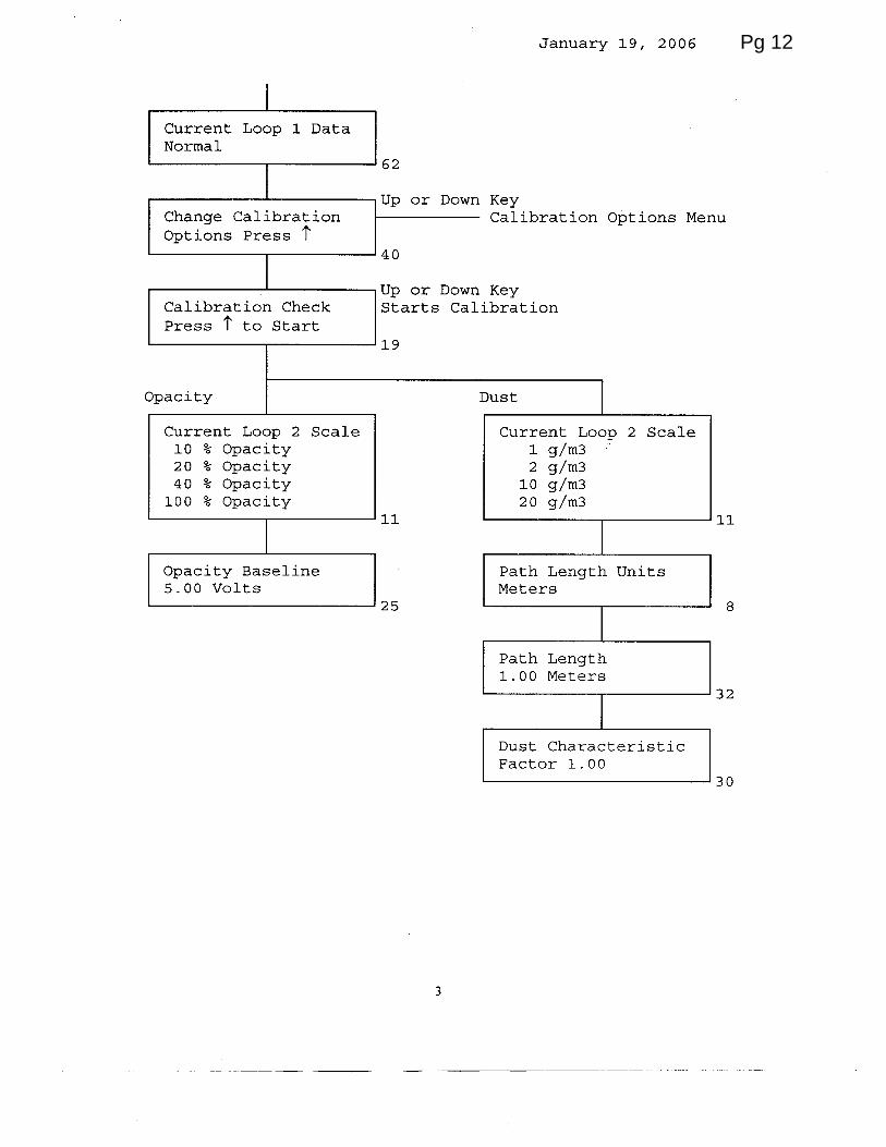
Pg 12
Pg 13

Pg 14
Pg 15

Pg 16

Pg 17
Pg 18

�����
�������������� ���������
������������������������������������������� ������������ ������!��"���������#$�����������������������%������%�&��'����� ��(��������#$�����)�%�����������������*����������%�������%��)���+,����-����������������*����������%�������%��)��!�+,����.��������#$�����)�%�����������������*����������%�������%���)��������������/!��������������*����������������00�� ������� ����������������������1���������������2�'3��������#$������*����������%�������%���)�������������(/-���������������*����������������00��������������� ����������������������14���������������*����������%����2�2���������������������

������

������
������
������

������

��������������� �������������������� ������� ���
����������� �������������� ��������� ���� �������
����� ��� ������� ��� ���� ���������� ��� ���� ��� ����
�������������������������
���� ������ ���� � � !�"� #$� �%��������� ������� �
������ ����������� &��� ���� ����� ����'��� � �������
����������� ���� ����������� ����'�� ��� ����������
���������������������
���� �������� �� ���� ����(���� ��� ���������
���������� ������ ���� �������� ��� ���� ���� ��
����'���)���������������������������������'��������
*+�)� ,���� ������ ��������� � -�� � ���� ����� ��� ����
������� ��� ����� �����./(01����� ���������� ����� ��� ����
���������
)��� ���� ��� �� ���������� ���������� ��������� ���,�
���������� ������� ��� �� �� ���� ������ ����'�� ��
������ �)��� ��������� ��� ��������� ���� ���� ���� ����
)���� ���(��������� � ������� ������ ������
������������������������������,��������
���� ���� �� ������ ���� �������� ��� �������������� ���� ��������
����� ��� ����� ������ � ����������� ������������ ������������
���� ����� ������ ��� � �������� ����� �� ��� ����� �� �������
��� ������ ���������� ������������������ ����� �������� ��� ��������
�������� � ��� ������������������������������������ ���������
������ ������� ���� �� � �� !��� !������ ������� ������� ���� ���
����� ���� ������� ���� ����� ��� �� �������� ������� ���
����� �������������������������� ����� ���� ������������ ��
������� ��� ������ ��� ��� ��� ���� "�#� !� � ��������� ���� ���
�������������������������
���� ������� ������������ ������$��� ����� ���� ��� ���� ��� ���
���!������� ������ ��� �%���� ����� ��� � ��� �������� ������� ��������
���������������������� ���� ������&���������������������������
#��� '������� �������������(�� ����������������� ������� ��� ����
����������� �����������)���")��#������������������������� �������
���� ������ *�+,� � � ��� ������� ������� � ���� ���- ����������� ���
��������� ������ ������� ������� ������ ���� ��� ����� �������� ���
��� ��������� ����� .����������� �������� ��� !�� ����� ��������
�� �������� ����� /)0 �� ��� ����������� ��� ��� ��� ����� �%������ �����
���������'�%���������������������!�����(�
������

������ �������� ��� ����������� ������������ ����
���� ���� �������� ������� ���� ������ ������� � ��� ��� ���
�������� ���� ���� ������ ��� ��� ����� �������� ���� �������
��� �� ���� ����� ���� ������� ����� ����� �� �� �� ��������������
������������ ���� ���� ������� �� ���� ��������� � ���� ���
���� � �� � !� "������ #$� ��������� ������� �����������
������������ � ���� ������� ����������� �����% �� ������ ��
��������� &����� ������ ��������� '&� (� ����������� ��
)���)� �������� ��� ��������������� � �* ������ � ��� �� �
����� �� ���� ������� ��� ������� ������ ��� ������ �����
��������� ��� ������������ ��������� � ���� ��� ����� �� ���
���� ���� *���� ������� *���� ��+���,������ � ���� ���� ��
� ���� ��������������������������
-� �������������.�������&����/������������������
���������.�������0������������ ��1����������� ����
������#2#3�43#��+�"!$��������
����� ���������������*�����������������#2#3�5#6����
������7���8�����*����������������'��9�433(��
"-�##:2�33��*��������"������'��"(����
������������#�����'5���% ���(
"-�36$2�33�;�����&�������"������';&"(����
���������<�#33��������4�������'5���% ���(�
#2#3�=3$�;������&>2����������� ����������*���
������

������������ ��
������������� ����� ����������������������������
������������ ����� ���!���"#�����������
$���������#������ %!&��� �!���#����&��&'()�*�������"+ �� �,����������
������#����������,�� %!&��� �!���#����&��&'-)�*�������"+ �� �,����������
.����������* ' )�������
������������ ��/���������"����������#��
$������0���#����� -�������1����������#������,��&��&���2������������
������3��� ��������� 0�����������*&���*,������"���*�������"�����"���
���������������������
���4!���!����������� ���� ��"�������&&������*�����*��� ��������
���������������!��������!3������ 5��**��������������
����������������� 6��7()������
$�#�������������!3������ &8��/�0�&8�� 8�9�!�& ��)����������
����� ������ �� �������
.�� ������ :��&��*�/;���,���#�����.:�"(������,������������
������3�����+!8<�� �8�*������2������ 7272 ���� ��" ��#��&&5:�$8+�� ���������
0�����6��=���4����>���������������5:�$8?����������������
(2 ;2-���� ��" ��#���*������������&��& -2 /2 ���� ��" (�#���*��������!*�����*��������
��� ��� ������ �� ������
6���@���*�����&-�-������@!����!��8&-��$�������������������������1$���+�����*�����������*��*����������#���������������
��+��*���������3��� 6��,����� ��&-8�>$0"(�!/�3A" ->$�*����B��������������
��+��*��0�����6�� 6��,����� ��&-8�>$0"(�!/�3A"8�>$�*����B��������������
0�#��#�+���0�����6��B�����,�3��� (*���������1����*����������� ������" ������"--$?C�
������������� ��� ������ ������ ���� ������
�������������������������� !�"�������#��$���%���&''��(�)�
*����+� ,-.+,+.+����/�+� ,-!&,!.'!�
��#����0�����1���� ��� ������ 1 �
����0������2���� ��� ������ 1 ��
������������������&� �?�� ��������������*������������� �������������������
��������� �����������������������������������������������������������������
������������ ����������������� ����������������� ��� ����� ������� ��������
��� ���*������������������������������������������� ��������� ������������
��������� ��*��������������������������������*����������������*����'��������
����� ���� �*������ ��������(� �������� ������� ���� �������� ���� ��� ���� ���
'����� ����9��������������������������*�� ���(�� ������������� ����������������
� �� ������ ����� *�� ���� ������� ����� ���� �������� ���� ���� ����� �������� ���
���������������� .�� ;.��&!����������������������������������������������������
����� ���� ���� ?� ��� �� $�53��!� � ������ ������ ����� �������� ��� ���� *�� ���� ���
���������������������������������������������������������������*�����������
������������ �����
������� ����������������������������
�����

Pg.28
301-963-3630 phone 301-948-4674 fax 2 Metropolitan Ct., Suite 6, Gaithersburg, MD 20878-4008 USA www.opticalscientific.com
OFS Technology Overview
1) Optical Scintillation (Light Fluctuation)
2) Temporal cross-correlation (i.e. Time of Flight)
Scintillation the refraction or diffraction of light through air pockets with different temperatures & densities (i.e. atmospheric turbulence). Optical scintillation induces light fluctuations. This phenomenon is a measurable atmospheric condition. The method employed to measure scintillation has been in use for over 30 years in atmospheric remote sensing. Examples of scintillation the light shim-mering off a blacktop road on a hot day or the twinkling of a star at night.
Temporal Cross-Correlation
Temporal Cross Correlation A Statistical Method to Measure Time of Flight: OFS measures the movement of scintillation Detector A senses the scintillation pattern first and then detector B senses the same pattern as it moves through the beam and past both detectors. OFS measures the time at which this pattern is detected at each point and knows the distance between the two detectors. Using advanced digital signal processing and temporal cross-correlation, OFS can calculate the velocity of the flow: Velocity = distance / time
The left-hand picture shows how light behaves without atmospheric turbulence (as in the vacuum of space). The right-hand picture demonstrates the diffusion of light (a.k.a. optical scintillation) caused by atmospheric turbulence, which exists in the air everywhere.
Detectors
OFS technology is independent of the media temperature, pressure, humidity & opacity!
Light without Atmospheric Turbulence
Light with Atmospheric Turbulence
Receiver Transmitter
LED
FLOW
Same scintillation pattern first detected by A, then
FLOW
Same scintillation pattern first detected by A then B
���������������������������� ������ �� �� ����� ��������������������������� ������� ��!���"������� ����#�$� �%%%����&���&�������&�&'
����� ����� ������������� ��� ��������
���� ��� ������������ �����������
����� ����� �������������� ����� ������
����� ���� ������������ �����������
����� ����� �������������� �������� ���
������ ��� �� ����� ������ �����������
������ ����� ����������� ������������
����� ���� ������ ����� ��� ��������
����� ��� � ������� ������ �� ��������
������ ������ �������������� �����������
������ ������ ������������ �������� ���
������������� �� ���������������������� �� ��
������������� �� ���������������� � � ��������� ���� �� �������� ��!�����"#��!�$��
%�&�������� � � ��������� ���� � ������������������� � ���������� ����������
��
���
���
���
���
���
�� ��� ��� ��� ��� ������� �� ��������
������������ �������
����������
�����
������