oscilloscope applications guidebook - pedro … · alternate trigger — a dual-trace ... when the...

Third Edition © 2001 B+K Precision Corp.

Oscilloscopes are often described as the most versatile piece of test equipment that a Technician or Engineer can use. The instrument provides an actual graph of voltage versus time on the screen. This type of graph is one of themost versatile "tools" for testing, analyzing, and troubleshooting electrical and electronic equipment because itallows you to actually measure instantaneous voltage levels and time periods of electrical signals. Additionally,oscilloscopes allow observation of amplitude changes (glitches), waveform distortion, and phase changes.Transducers can also be used adapt the oscilloscope to measure such things as mechanical stress, heat, gaspressure, fluid pressure, light, weight, or just about anything else that a transducer can convert to an electrical signal.Although applications for oscilloscopes are virtually unlimited, here are just a few of the more common uses:

• FIELD ENGINEERING.• RESEARCH AND DEVELOPMENT.• SECONDARY AND POST SECONDARY EDUCATIONAL INSTITUTIONS.• ELECTRONIC AND ELECTRICAL EQUIPMENT REPAIRS SHOPS.• CONSUMER PRODUCTS REPAIR SHOPS.• GOVERNMENT REPAIR FACILITIES.

In order to use an oscilloscope to its best advantage, the Technician and Engineer should have a basic under-standing of how an oscilloscope works as well as a good understanding of the oscilloscope’s controls, features,and operating modes. This guidebook is useful to those with little knowledge of oscilloscopes as well as the expe-rienced technician or engineer who wishes to refresh their memory or explore new uses for oscilloscopes.

1031 Segovia Circle, Placentia, CA 92870-7137

OSCILLOSCOPEAPPLICATIONS

GUIDEBOOK

TABLE OF CONTENTSOSCILLOSCOPE GUIDE

All rights reserved. No part of this guidebook shall be reproduced, stored in a retrieval system, or transmitted by any means, electronic, mechanical,photocopying, recording, or otherwise, without permission from B+K PRECISION. While extensive precautions have been taken in the preparation of thisguidebook to assure accuracy, B+K PRECISION assumes no responsibility for errors or omissions. Neither is any liability assumed for damages resulting from the use of the information contained herein.

COMMON OSCILLOSCOPE TERMS . . . . . . . . . . . . . . . . . . . . . . . . . . . . . . . . . . . . . . . . . . . . . . . . . . . . . . . . . .1

OSCILLOSCOPE SAFETY . . . . . . . . . . . . . . . . . . . . . . . . . . . . . . . . . . . . . . . . . . . . . . . . . . . . . . . . . . . . . . . . . . .3

CONTROLS AND INDICATORS . . . . . . . . . . . . . . . . . . . . . . . . . . . . . . . . . . . . . . . . . . . . . . . . . . . . . . . . . . . . . .4

Basic Analog Oscilloscopes . . . . . . . . . . . . . . . . . . . . . . . . . . . . . . . . . . . . . . . . . . . . . . . . . . . . . . . . . . . . . .4

Advanced Analog Oscilloscopes . . . . . . . . . . . . . . . . . . . . . . . . . . . . . . . . . . . . . . . . . . . . . . . . . . . . . . . . . .6

Digital Storage Oscilloscopes (DSO) . . . . . . . . . . . . . . . . . . . . . . . . . . . . . . . . . . . . . . . . . . . . . . . . . . . . . . .7

OPERATING AN OSCILLOSCOPE . . . . . . . . . . . . . . . . . . . . . . . . . . . . . . . . . . . . . . . . . . . . . . . . . . . . . . . . . . . .8

Basic Analog Oscilloscopes . . . . . . . . . . . . . . . . . . . . . . . . . . . . . . . . . . . . . . . . . . . . . . . . . . . . . . . . . . . . . .8

Advanced Analog Oscilloscopes . . . . . . . . . . . . . . . . . . . . . . . . . . . . . . . . . . . . . . . . . . . . . . . . . . . . . . . . .12

Digital Storage Oscilloscopes (DSO) . . . . . . . . . . . . . . . . . . . . . . . . . . . . . . . . . . . . . . . . . . . . . . . . . . . . . .14

HOW OSCILLOSCOPE WORK . . . . . . . . . . . . . . . . . . . . . . . . . . . . . . . . . . . . . . . . . . . . . . . . . . . . . . . . . . . . . .17

Basic Analog Oscilloscopes . . . . . . . . . . . . . . . . . . . . . . . . . . . . . . . . . . . . . . . . . . . . . . . . . . . . . . . . . . . . .17

Advanced Analog Oscilloscopes . . . . . . . . . . . . . . . . . . . . . . . . . . . . . . . . . . . . . . . . . . . . . . . . . . . . . . . . .20

Digital Storage Oscilloscopes (DSO) . . . . . . . . . . . . . . . . . . . . . . . . . . . . . . . . . . . . . . . . . . . . . . . . . . . . . .22

OSCILLOSCOPE PROBES . . . . . . . . . . . . . . . . . . . . . . . . . . . . . . . . . . . . . . . . . . . . . . . . . . . . . . . . . . . . . . . . . .24

APPLICATIONS . . . . . . . . . . . . . . . . . . . . . . . . . . . . . . . . . . . . . . . . . . . . . . . . . . . . . . . . . . . . . . . . . . . . . . . . . . .25

Basic Oscilloscope Applications . . . . . . . . . . . . . . . . . . . . . . . . . . . . . . . . . . . . . . . . . . . . . . . . . . . . . . . . .25

Delayed Sweep Applications . . . . . . . . . . . . . . . . . . . . . . . . . . . . . . . . . . . . . . . . . . . . . . . . . . . . . . . . . . . .37

DSO Applications . . . . . . . . . . . . . . . . . . . . . . . . . . . . . . . . . . . . . . . . . . . . . . . . . . . . . . . . . . . . . . . . . . . .39

The NTSC Color Video Signal . . . . . . . . . . . . . . . . . . . . . . . . . . . . . . . . . . . . . . . . . . . . . . . . . . . . . . . . . .40

Page

OSCILLOSCOPE GUIDE

1

ACCELERATING VOLTAGE — The inter-nal voltage that accelerates the electron beamand causes trace illumination on the oscillo-scope display. A higher voltage causes abrighter trace. Oscilloscopes with higher band-width need a higher accelerating voltage tomake the trace visible when viewing high fre-quency signals. Usually measured in kilovolts(kV).

ALIASING — A phenomenon which occurs inreal-time sampling on a DSO when the samplingrate is too low for reliable sampling. Aliasingproduces a display which looks valid but is infact totally erroneous in terms of time measure-ment.

ALTERNATE SWEEP — A method of gen-erating dual trace display at higher sweepspeeds. In this method, one entire trace isdrawn, then the other, in an alternating fashion.See "Chop".

ALTERNATE TRIGGER — A dual-tracetriggering scheme in which the channel 1 signaltriggers the channel 1 trace, and the channel 2signal triggers the channel 2 trace in an alter-nate pattern. Thus, each signal becomes its owntrigger source, and a synchronized display canbe obtained even if the two signals have no timerelationship.

ATTENUATION — A decrease in signalamplitude. Usually measured in decibels (dB).

BANDWIDTH — The frequency range ofsignals that can be observed on the oscillo-scope with minimum degradation. Typically,bandwidth is specified in megahertz (MHz) andis the maximum frequency at which signals arewithin 3 dB in amplitude. A 20 MHz oscilloscopehas a bandwidth of dc to 20 MHz. This meansthat a 20 MHz oscilloscope can be used tomeasure amplitude of a 20 MHz signal and willprovide a measurement with a maximum of 3dB (decibels) of attenuation compared to a ref-erence frequency of 1 kHz. Since oscilloscopesare usually conservatively rated, less then 3 dBof attenuation will typically be experienced at themaximum rated bandwidth.

BLANKING — Turning off the CRT electronbeam. An oscilloscope CRT is "unblanked" dur-ing the trace and "blanked" during the re-traceand while waiting for a trigger.

CHANNEL — The complete input circuitry,including the vertical attenuator, vertical amplifi-er. and input coupling network, for a single sig-nal. Typically, modern oscilloscopes have two ormore channels and therefore have two or morevertical attenuators, vertical amplifiers, and inputcoupling networks.

CHOP SWEEP — A method of generatingdual-trace display at lower sweep speeds. Inthis method, the electron beam jumps from onetrace to the other, drawing a small bit of each,as it makes its way across the screen.

COMPONENT TEST — A feature on someadvanced analog oscilloscopes which allowstesting of components in-circuit or out-of-circuit.When the component test mode is selected,normal sweep is disabled and the oscilloscopedisplays a pattern representing the dynamicimpedance of the component when a 60 Hz sinewave is applied.

CROSSTALK — Sometimes referred to aschannel isolation or channel separation. Theundesired effect that a signal present on onechannel has on another channel. Less crosstalkmeans that the channels are better isolated fromone another. Usually expressed in dB.

CRT — Abbreviation for Cathode Ray Tube.The cathode ray tube is similar to a televisionpicture tube and acts as the oscilloscope display.

DECIBEL (dB) — A unit of measurementusually used to show a ratio of input signalpower or voltage to output signal power or volt-age. Decibels are calculated by taking the log ofthe output power divided by the input power andmultiplying that by 10. This can be expressed bythe equation dB = 10 log (Output Power / InputPower).

DELAYED TIME BASE — A delayed timebase oscilloscope allows a single signal to heviewed at two different time bases with the sec-ond time base expanding a portion of the wave-form and starting at some point after the maintime base begins. This type of display is moreuseful than merely magnifying the displaybecause it allows simultaneous viewing of themain sweep signal and the expanded signal,and allows any desired degree of magnification.

DIGITAL STORAGE OSCILLOSCOPE— An oscilloscope that uses computer technolo-gy to digitize and store waveforms. This type ofspecialized scope is very useful for capturingand viewing extremely slow events, one-timeevents, and pre-trigger events. It can also pro-vide disk storage and hard copy of a waveformthrough a computer/plotter interface.

DIGITIZE — To convert an analog quantity todigital. A DSO digitizes an analog voltageapplied to its input and converts it to a series ofdigital numbers which are stored in memory.

DSO — Abbreviation for "Digital StorageOscilloscope".

DUAL TRACE — An oscilloscope having twotraces to display channel 1 and channel 2 signals simultaneously.

EQUIVALENT TIME SAMPLING —Method of sampling used on a DSO, whereinsampling is synchronized with the trigger signal,usually one sample per cycle of the input.Samples are taken at slightly increasing inter-vals after each trigger, so that one completecycle is stored after many cycles of the input.Equivalent time sampling allows a waveform tobe digitized using a much lower sampling rate,but the waveform must he repetitive. See "RealTime Sampling".

FALLTIME — The time required for a signalto fall from 90% to 10% of its maximum ampli-tude. Faster fall times cause steeper trailingedges of pulses, usually a desirable trait. Therise time specification for an oscilloscope canalso be used as the fall time specification. See"Rise Time" for further explanation.

GRATICULE — The graph, usually etchedon the inside of the CRT, that allows time andvoltage measurements to be taken.

INTENSITY MODULATION — See "Z-Axis".

LINEARITY — A perfectly linear sweepwould be produced by a perfectly linear sweepramp. This means that any variance in thesweep ramp would cause the time representedby one horizontal division on the display (e.g.the leftmost division) to be unequal to the time

COMMON OSCILLOSCOPE TERMS

OSCILLOSCOPE GUIDE

2

represented by another horizontal division onthe display (e.g. the rightmost division).

PHOSPHOR — A coating on the inside ofthe CRT that emits visible light when struck withan electron beam. Oscilloscope CRTs usuallyuse a P31-type phosphor, which is a short-per-sistence type; that is, the emitted light quenchessoon after the electron beam ceases or moves.

POST-TRIGGER DATA — Data whichoccurred after the event that caused a DSO totrigger.

PRE-TRIGGER DATA — Data whichoccurred before the event that caused a DSO totrigger. Modern DSOs allow the user to viewsuch data.

REAL TIME SAMPLING — Method ofsampling used on a DSO, wherein the samplesare taken at regular intervals that are deter-mined by the sweep time setting. The samplingprocess proceeds independently of the input.The sampling rate must be at least twice the fre-quency of the input for meaningful waveformacquisition to occur. See "Equivalent TimeSampling".

RISE TIME — The time required for a signalto rise from 10% to 90% of its maximum ampli-tude. Faster rise times cause steeper leadingedges of pulses, usually a desirable trait. Therise time specification for an oscilloscope refersto the minimum time that it takes the CRT beamto rise from the 10% mark on the CRT graticuleto the 90% mark on the graticule. Oscilloscoperise time specifications are directly related tobandwidth.

SAMPLING — The process of digitizing on aDSO. Every time the scope "samples" an inputwaveform, it memorizes the voltage value at thatinstant and converts it to a binary number whichcan be stored in memory.

SAMPLING RATE — The rate at whichsampling occurs in a DSO, usually expressed insamples per second. DSOs are typically ratedby their maximum sampling rate, usuallyexpressed in megasamples per second.

SWEEP — The motion of the CRT electronbeam from left to right that causes the trace toappear. A sweep time of 0.1mS/div means that

the beam moves across one division of the CRTin 0.1mS. Faster sweep speeds are required toview higher frequency signals. If the frequencyof the input signal remains constant and thesweep speed is increased, the number of cycles(or portion of the waveform) that are displayedon the CRT will decrease (effectively magnifyingthe display).

SWEEP MAGNIFIER — Sometimesreferred to as sweep expander. This featureallows a portion of a displayed waveform to bemagnified (typically x10) without shortening thesweep time setting. This is an advantage oversimply increasing the sweep speed becausedoing so can result in the desired portion of thewaveform disappearing off the screen.Additionally, this feature increases the maximumsweep speed by the magnification factor (i.e. ifthe fastest sweep time/div setting of an oscillo-scope is 0.5 mS/div and x10 magnification isselected, the sweep speed is increased to 0.05mS/div).

TIME BASE — The calibrated sweep genera-tor circuit within the oscilloscope which allowsmeasurement of signal time period and frequen-cy. The time base is calibrated in time/div. Inother words, if the time base is 10 mS/div, itwould take 100 mS for the electron beam tosweep across all 10 of the CRT’s horizontal divi-sions.

TRIGGER — In an analog oscilloscope, theevent or signal that causes the CRT beam tobegin its sweep across the display. In a DSO,the event around which the storage process isreferenced. Some DSOs place the trigger in thecenter of the storage memory, so that there areequal amounts of pre- and post-trigger datastored. In both analog and digital scopes, greatversatility is provided in setting the triggersource, level, and slope.

TV SYNC — see "Video Sync".

VERTICAL MAGNIFICATION — A fea-ture on many oscilloscopes in which the verticalinput signal is amplified, or magnified. The typi-cal magnification factor is 5 times. This increas-es sensitivity and makes the oscilloscope moreuseful for measuring very low level signals.

VERTICAL SENSITIVITY — The signallevel required to cause a single division of verti-cal deflection. For example, for a vertical attenu-ator setting of 5 mV/div, a 5 mV peak signal willproduce a single division of vertical deflection.

VERTICAL ATTENUATOR — The preci-sion input circuit that controls the level of theinput signal so that the signal provides anamount of vertical deflection that can be easilymeasured on the CRT screen. Usually this cir-cuit consists of calibrated steps in a 1-2-5sequence (10 mV/div, 20 mV/div, 50 mV/div,etc.), which allow the oscilloscope to display sig-nals with levels from many volts to only a fewmillivolts.

VIDEO SYNC — Sometimes referred to asTV sync. This feature allows vertical (TV V) orhorizontal (TV H) video sync pulses to beselected for triggering. Vertical sync pulses areselected to view vertical fields or frames ofvideo and horizontal sync pulses are selectedfor viewing horizontal lines of video.

X-AXIS — The horizontal axis, when oscillo-scope is not in sweep mode.

X-Y DISPLAY — Mode of operation whichdisplays a graph of two voltages. The Y axis isthe vertical axis and the X-axis is the horizontalaxis.

Y-AXIS — The vertical axis.

Y-AXIS OUTPUT — A sample of the verti-cal axis signal which is available at a rear paneloutput jack.

Z-AXIS — Also referred to as intensity modu-lation. This feature allows an external signal tocontrol the intensity of the CRT beam.

OSCILLOSCOPE SAFETY — The ac anddc resistance that a signal "sees" at the oscillo-scope input. Typically, input impedance isexpressed in terms of dc resistance (measuredin megohms) and capacitance (measured inpicofarads).

Common Oscilloscope Terms

OSCILLOSCOPE GUIDE

3

Review and follow the guidelines on this page touse your oscilloscope safely and responsibly.

Preventing Electric Shock

1. Using an oscilloscope may often involve working inside equipment that contains highvoltage. Under such conditions, you should observe the following:

a. Don’t expose high voltage needlessly.

b. Be familiar with the location of the high voltage points, and remember that high voltage may appear at an unexpected point in effective equipment.

c. Use an insulated floor material orinsulated work surface.

d. Keep one hand in your pocket when using a scope probe.

e. Remember that ac power may be present in the equipment even when it is turned off.

f. Use an isolation transformer whenever the equipment’s power plug is two-prong only.

g. Have someone nearby, preferably with CPR training.

2. Don’t operate the oscilloscope with the cover removed.

3. Keep the scope grounded with the 3-wire power plug. Don’t attempt to defeat the third prong or "float" the scope.

Preventing Damage to theOscilloscope

1. Don’t leave the oscilloscope set at high brightness for long intervals. A bright spot or line left in one position can permanently burn the screen.

2. Keep the ventilation holes clear.

3. Don’t apply excessive voltage to the scope’s input jacks. Voltage limits are clearly stated in your operating manual and usually on the scope itself.

4. Connect the ground clip of a scope probe only to earth ground or isolated common in the equipment under test.

5. Keep the scope away from:

a. Direct sunlight.

b. High temperature/humidity.

c. Mechanical vibration.

d. Electrical noise and strong magnetic fields.

Oscilloscope Safety

OSCILLOSCOPE GUIDE

4

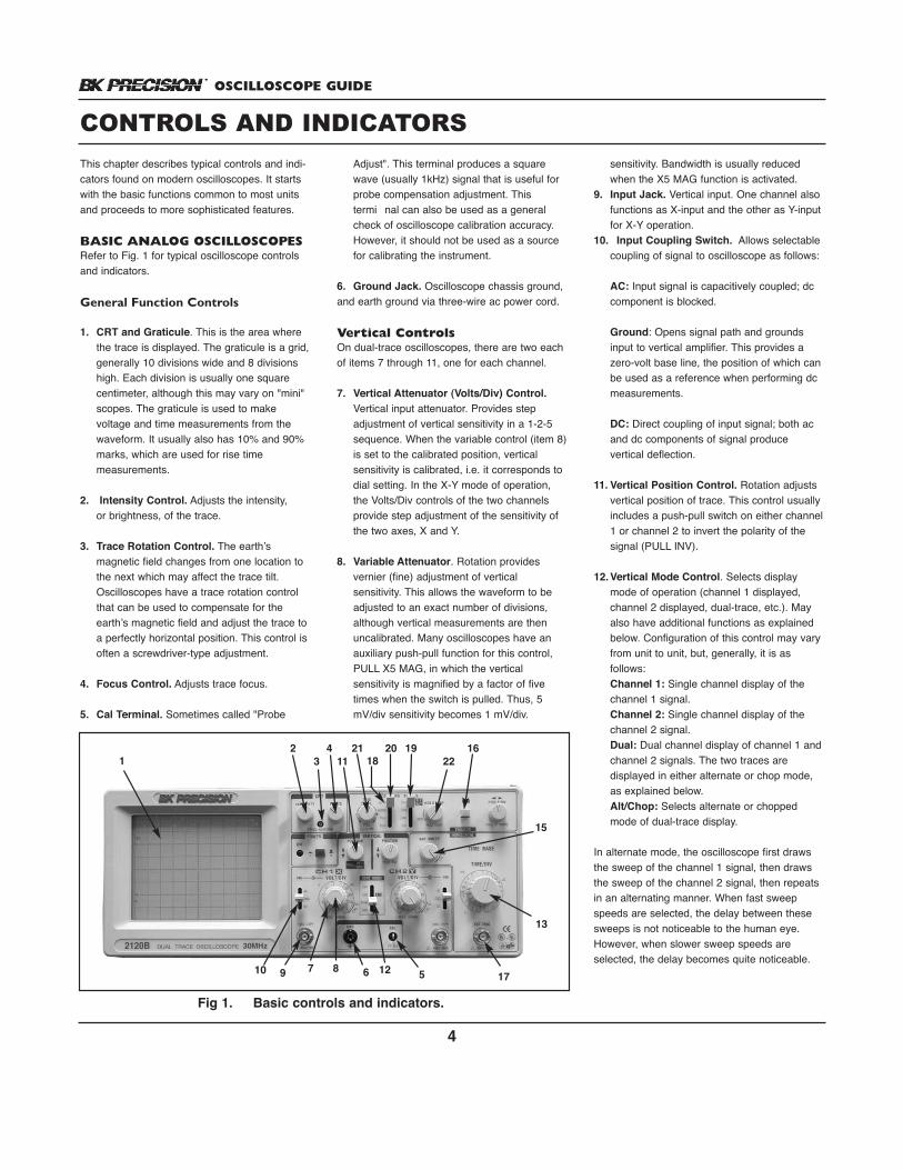
This chapter describes typical controls and indi-cators found on modern oscilloscopes. It startswith the basic functions common to most unitsand proceeds to more sophisticated features.

BASIC ANALOG OSCILLOSCOPESRefer to Fig. 1 for typical oscilloscope controlsand indicators.

General Function Controls

1. CRT and Graticule. This is the area where the trace is displayed. The graticule is a grid,generally 10 divisions wide and 8 divisions high. Each division is usually one square centimeter, although this may vary on "mini" scopes. The graticule is used to make voltage and time measurements from the waveform. It usually also has 10% and 90% marks, which are used for rise time measurements.

2. Intensity Control. Adjusts the intensity, or brightness, of the trace.

3. Trace Rotation Control. The earth’s magnetic field changes from one location to the next which may affect the trace tilt. Oscilloscopes have a trace rotation control that can be used to compensate for the earth’s magnetic field and adjust the trace to a perfectly horizontal position. This control isoften a screwdriver-type adjustment.

4. Focus Control. Adjusts trace focus.

5. Cal Terminal. Sometimes called "Probe

Adjust". This terminal produces a square wave (usually 1kHz) signal that is useful for probe compensation adjustment. This termi nal can also be used as a general check of oscilloscope calibration accuracy. However, it should not be used as a source for calibrating the instrument.

6. Ground Jack. Oscilloscope chassis ground, and earth ground via three-wire ac power cord.

Vertical ControlsOn dual-trace oscilloscopes, there are two eachof items 7 through 11, one for each channel.

7. Vertical Attenuator (Volts/Div) Control.Vertical input attenuator. Provides step adjustment of vertical sensitivity in a 1-2-5 sequence. When the variable control (item 8)is set to the calibrated position, vertical sensitivity is calibrated, i.e. it corresponds to dial setting. In the X-Y mode of operation, the Volts/Div controls of the two channels provide step adjustment of the sensitivity of the two axes, X and Y.

8. Variable Attenuator. Rotation provides vernier (fine) adjustment of vertical sensitivity. This allows the waveform to be adjusted to an exact number of divisions, although vertical measurements are then uncalibrated. Many oscilloscopes have an auxiliary push-pull function for this control, PULL X5 MAG, in which the vertical sensitivity is magnified by a factor of five times when the switch is pulled. Thus, 5 mV/div sensitivity becomes 1 mV/div.

sensitivity. Bandwidth is usually reduced when the X5 MAG function is activated.

9. Input Jack. Vertical input. One channel also functions as X-input and the other as Y-inputfor X-Y operation.

10. Input Coupling Switch. Allows selectable coupling of signal to oscilloscope as follows:

AC: Input signal is capacitively coupled; dc component is blocked.

Ground: Opens signal path and grounds input to vertical amplifier. This provides a zero-volt base line, the position of which canbe used as a reference when performing dc measurements.

DC: Direct coupling of input signal; both ac and dc components of signal produce vertical deflection.

11. Vertical Position Control. Rotation adjusts vertical position of trace. This control usually includes a push-pull switch on either channel1 or channel 2 to invert the polarity of the signal (PULL INV).

12. Vertical Mode Control. Selects display mode of operation (channel 1 displayed, channel 2 displayed, dual-trace, etc.). May also have additional functions as explained below. Configuration of this control may vary from unit to unit, but, generally, it is as follows:Channel 1: Single channel display of the channel 1 signal.Channel 2: Single channel display of the channel 2 signal.Dual: Dual channel display of channel 1 andchannel 2 signals. The two traces are displayed in either alternate or chop mode, as explained below.Alt/Chop: Selects alternate or chopped mode of dual-trace display.

In alternate mode, the oscilloscope first drawsthe sweep of the channel 1 signal, then drawsthe sweep of the channel 2 signal, then repeatsin an alternating manner. When fast sweepspeeds are selected, the delay between thesesweeps is not noticeable to the human eye.However, when slower sweep speeds areselected, the delay becomes quite noticeable.

CONTROLS AND INDICATORS

Fig 1. Basic controls and indicators.

12

34

11 1821 20 19

12

2216

15

13

10 9 7 8 6 5 17

OSCILLOSCOPE GUIDE

5

In chop mode, the oscilloscope draws a smallpart of the channel 1 signal, then a small part ofthe channel 2 signal, and so on, continuallyswitching back and forth until both sweeps arecompleted. The switching rate is very fast, andthis "chopping" is not noticeable to the humaneye when slow sweep speeds are selected.

Note:Some oscilloscopes automatically select chop oralternate display based on the setting of thetime base control, enabling chopped display atslower sweep speeds and alternating display atfaster speeds.

Add: The channel 1 and channel 2 signals are algebraically combined, and the result is displayed on the CRT as a single trace. Thiscombined signal then represents channel 1 plus channel 2. If one channel is inverted, say channel 2, the result is the algebraic difference, channel 1 minus channel 2.

Horizontal Controls — SweepGroup

13. Time Base (Time/Div) Control. Provides step selection of sweep rate for the time base. As with the vertical attenuator, steps are arranged in a 1-2-5 sequence. When the variable time base control (item 14) is set to the calibrated position, sweep rate is calibrated, i.e. it corresponds to dial setting.

14. Variable Time Base Control. Rotation of this control provides vernier (fine) adjustment of the sweep rate. This allows the waveform to be adjusted to an exact number of divisions, although horizontal meas urements are then uncalibrated.

15. Horizontal Position / X10 MagnificationControl.

Horizontal Position: Rotation controls horizontal position of trace.

X10 Magnification: Selects ten times sweep magnification, i.e. if time base is set to 0.1 mS/div, selecting X10 magnification increases this setting to 10nS/div. This is useful for closer inspection of a specific partof the waveform.

16. X-Y Switch. Selects X-Y operating mode.

In X-Y operation, the CRT display becomes an electronic graph of two instantaneous voltages. One input channel is displayed on the X-axis, and the other on the Y-axis.

Horizontal Controls — Triggering Group

17. External Trigger Input Jack. This input allows an external signal to be applied as the trigger source.

18. Automatic-Normal Trigger Control:Selects automatic triggering mode, wherein the scope generates a sweep (free runs) in the absence of an adequate trigger signal. Itautomatically reverts to triggered sweep operation when an adequate trigger signal is present. Auto triggering differs from normal triggered operation in that in normal operation, the sweep does not trigger when a trigger signal is not present. Auto-triggering is handy when first setting up the unit to observe a waveform.

19. Trigger Source Switch. Selects the source of the sweep trigger. Some common trigger sources are:

Channel 1: The channel 1 input signal becomesthe sweep trigger, regardless of the vertical mode control setting.

Channel 2: The channel 2 input signal becomesthe sweep trigger, regardless of the vertical mode control setting.

Alternate: The trigger source alternates between the two traces in dual-trace operation.

External: The signal connected to the external trigger input jack becomes the trigger signal.

20. Trigger Coupling Switch. Selects the method by which the trigger signal is coupled to the triggering circuits. Several common trigger coupling modes are:

AC: Trigger signal is capacitively coupled; dc component is blocked.

DC: Trigger signal is direct-coupled. Used for low-frequency (below 20Hz) triggering or to stabilize triggering on a signal with ac and

dc components. Not available on all scopes.

TV-H (HF): Used for triggering from video horizontal sync pulses. Also sometimes serves as low frequency reject coupling.

TV-V (LF): Used for triggering from video vertical sync pulses. Also sometimes servesas high frequency reject coupling.

LINE: Signal derived from input line voltage (50/60 Hz) becomes trigger.

21. Trigger Level / Slope Switch.Trigger Level Control: Determines the point on

the waveform where the sweep is triggered.Rotation in the (–) direction selects more negative point of triggering, and rotation in the (+) direction selects more positive. Note that rotation too far in either direction may inhibit triggering completely.

Trigger Slope Switch: Selects positive-going slope or negative-going slope as the triggering point on the trigger waveform. In many scopes this control is implemented asa push-pull action on the Triggering Level control. Rear Panel Controls (not shown)Fuse Holder/Line Voltage Selector. Containsfuse and selects line voltage. Sometimes a separate control is used to select line voltage, or, in the case of a switching type power supply, no selection is necessary.


OSCILLOSCOPE GUIDE

6

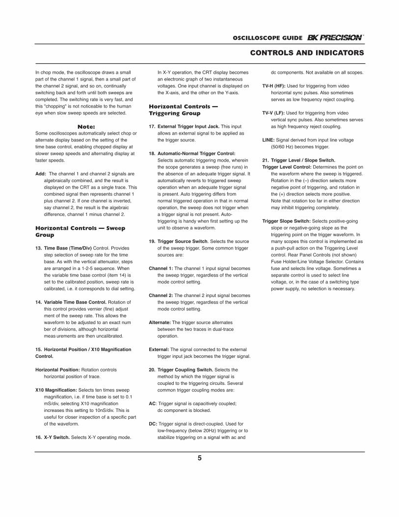
Refer to Fig. 2. Higher-end analog oscilloscopesoffer a host of features more advanced thanthose found on basic units. The most prominentadvanced features are increased bandwidth,delayed sweep, and component test. Othersinclude variable holdoff, Z-axis (intensity) modu-lation, bandwidth limiter, and scale illumination.

22. Holdoff Control. Adjusts holdoff time, whichis a period after each sweep is completed during which the next sweep is inhibited. Useful for stabilizing complex waveforms that have several possible triggering points.

23. Sweep Mode Switch. Enables the various modes of delayed sweep operation.

Main: Only the main sweep is displayed; the delayed sweep is blanked.

Delay: Only the delayed sweep is displayed.

MIX: The main and delayed sweep share a single trace; the main sweep occupies the left portion of the display, while the delayed sweep occupies the right portion of the display. The "Delay Time" control determines the starting point of the delayed sweep, that is, the percentage of the displaythat is main sweep and the percentage of the display that is delayed sweep. The mainsweep is often brighter than the delayed sweep due to the faster moving beam of thedelayed sweep. Delayed sweep cannot be slower than the main sweep.

X-Y: Most delayed-sweep oscilloscopes locate the X-Y switch in this grouping of controls.This switch enables X-Y operating mode as previously mentioned under item 16.

24. Main Time Base (Time/Div) Control.Same as item 13. Provides step selection of sweep rate for the main time base.

25. Delayed Time Base (Time/Div) Control.Provides step selection of sweep rate for the delayed sweep. For meaningful resultswith delayed sweep, this control should beset to a faster sweep speed than the mainsweep time.

26. Delayed Position Control. Adjusts the starting point of the delayed sweep with respect to the start of the main sweep. Sometimes implemented as a rotational control, sometimes as a press-and-hold electronic switch.

27. Scale Illumination Control. On oscilloscopes that have a lighted graticule,this control is provided to control the brightness of that illumination.( Not shown)

28. Beam Finder Switch. This function, foundon some units, compresses the vertical and horizontal size of the trace and brings it toward the center of the CRT. This is useful when setting up the oscilloscope and the trace can’t be located because theamplitude of the signal pushes the trace off the CRT (or the position controls have been incorrectly adjusted).

29. Component Test Jacks. Usually two banana jacks; provide input for componenttest function that produces a component "signature" on the CRT by applying an ac signal across a device. Rather than the usual oscilloscope display of voltage versus time, the display shows a graph of voltage versus current. The signatures thus produced are characteristic of the device being tested — resistor, capacitor, etc., and can be used to detect defective components.

30. Component Test Switch. Turns component test mode on or off.

Additional Controls (not shown in the figure):

Bandwidth Limiter. Reduces the bandwidth of some high-frequency models. Helps to eliminate radio-frequencynoise when making low-frequency measurements.

Y-Axis Output Jack (on rear panel).Output terminal where a sample of the channel 2 (may be channel 1 on some oscilloscopes) is available. Amplitude of this signal is usually 50 mV/div of vertical deflection on the CRT, when terminated into 50 ohms. Useful for triggering frequency counters from a low level signal.

Z-Axis Input Jack (on rear panel).Sometimes called "External Blanking Input". Input jack for intensity modulation of the CRT electron beam.


ADVANCED ANALOG OSCILLOSCOPES

Fig 2. Controls on an advanced analog oscilloscope.

22 23

2830 29

26

26

24

OSCILLOSCOPE GUIDE

7

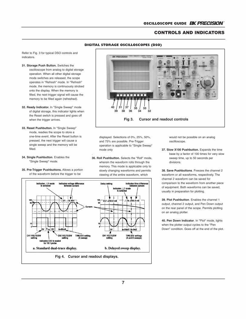
displayed. Selections of 0%, 25%, 50%, and 75% are possible. Pre-Trigger operation is applicable to "Single Sweep" mode only

.36. Roll Pushbutton. Selects the "Roll" mode,

wherein the waveform rolls through the memory. This mode is applicable only to slowly changing waveforms and permits viewing of the entire waveform, which

Refer to Fig. 3 for typical DSO controls and indicators.

31. Storage Push Button. Switches the oscilloscope from analog to digital storage operation. When all other digital storage mode switches are released, the scope operates in "Refresh" mode. In "Refresh" mode, the memory is continuously strobedonto the display. When the memory is filled, the next trigger signal will cause the memory to be filled again (refreshed).

32. Ready Indicator. In "Single Sweep" mode of digital storage, this indicator lights whenthe Reset switch is pressed and goes off when the trigger arrives.

33. Reset Pushbutton. In "Single Sweep" mode, readies the scope to store a one-time event. After the Reset button is pressed, the next trigger will cause a single sweep and the memory will be filled.

34. Single Pushbutton. Enables the "Single Sweep" mode.

35. Pre-Trigger Pushbuttons. Allows a portion of the waveform before the trigger to be

would not be possible on an analog oscilloscope.

37. Slow X100 Pushbutton. Expands the time base by a factor of 100 times for very slowsweep time, up to 50 seconds per divisions.

38. Save Pushbuttons. Freezes the channel 2waveform or all waveforms, respectively. Thechannel 2 waveform can be saved for comparison to the waveform from another pieceof equipment. Both waveforms can be saved, usually in preparation for plotting.

39. Plot Pushbutton. Enables the channel 1output, channel 2 output, and Pen Down outputon the rear panel of the scope. Permits plottingon an analog plotter.

40. Pen Down Indicator. In "Plot" mode, lightswhen the plotter output cycles to the "PenDown" condition. Goes off at the end of the plot.


DIGITAL STORAGE OSCILLOSCOPES (DSO)

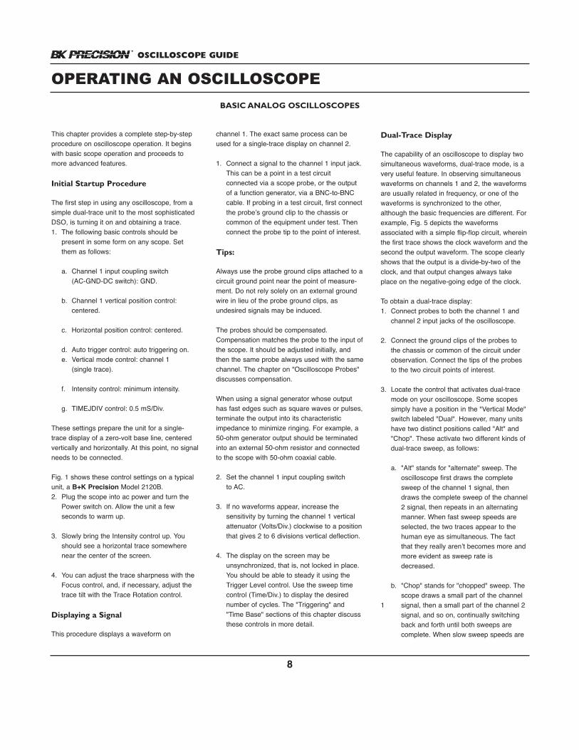
Fig 4. Cursor and readout displays.

Fig 3. Cursor and readout controls

40 31 37 35 3339 38 36 34 32

OSCILLOSCOPE GUIDE

8

This chapter provides a complete step-by-stepprocedure on oscilloscope operation. It beginswith basic scope operation and proceeds tomore advanced features.

Initial Startup Procedure

The first step in using any oscilloscope, from asimple dual-trace unit to the most sophisticatedDSO, is turning it on and obtaining a trace.1. The following basic controls should be

present in some form on any scope. Set them as follows:

a. Channel 1 input coupling switch (AC-GND-DC switch): GND.

b. Channel 1 vertical position control: centered.

c. Horizontal position control: centered.

d. Auto trigger control: auto triggering on.e. Vertical mode control: channel 1

(single trace).

f. Intensity control: minimum intensity.

g. TIMEJDIV control: 0.5 mS/Div.

These settings prepare the unit for a single-trace display of a zero-volt base line, centeredvertically and horizontally. At this point, no signalneeds to be connected.

Fig. 1 shows these control settings on a typicalunit, a B+K Precision Model 2120B.2. Plug the scope into ac power and turn the

Power switch on. Allow the unit a few seconds to warm up.

3. Slowly bring the Intensity control up. You should see a horizontal trace somewhere near the center of the screen.

4. You can adjust the trace sharpness with the Focus control, and, if necessary, adjust the trace tilt with the Trace Rotation control.

Displaying a Signal

This procedure displays a waveform on

channel 1. The exact same process can beused for a single-trace display on channel 2.

1. Connect a signal to the channel 1 input jack. This can be a point in a test circuit connected via a scope probe, or the output of a function generator, via a BNC-to-BNC cable. If probing in a test circuit, first connectthe probe’s ground clip to the chassis or common of the equipment under test. Then connect the probe tip to the point of interest.

Tips:

Always use the probe ground clips attached to acircuit ground point near the point of measure-ment. Do not rely solely on an external groundwire in lieu of the probe ground clips, as undesired signals may be induced.

The probes should be compensated.Compensation matches the probe to the input ofthe scope. It should be adjusted initially, andthen the same probe always used with the samechannel. The chapter on "Oscilloscope Probes"discusses compensation.

When using a signal generator whose outputhas fast edges such as square waves or pulses,terminate the output into its characteristicimpedance to minimize ringing. For example, a50-ohm generator output should be terminatedinto an external 50-ohm resistor and connectedto the scope with 50-ohm coaxial cable.

2. Set the channel 1 input coupling switch to AC.

3. If no waveforms appear, increase the sensitivity by turning the channel 1 vertical attenuator (Volts/Div.) clockwise to a positionthat gives 2 to 6 divisions vertical deflection.

4. The display on the screen may be unsynchronized, that is, not locked in place. You should be able to steady it using the Trigger Level control. Use the sweep time control (Time/Div.) to display the desired number of cycles. The "Triggering" and "Time Base" sections of this chapter discuss these controls in more detail.

Dual-Trace Display

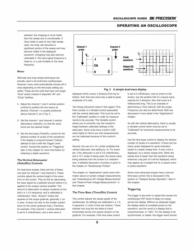
The capability of an oscilloscope to display twosimultaneous waveforms, dual-trace mode, is avery useful feature. In observing simultaneouswaveforms on channels 1 and 2, the waveformsare usually related in frequency, or one of thewaveforms is synchronized to the other,although the basic frequencies are different. Forexample, Fig. 5 depicts the waveforms associated with a simple flip-flop circuit, whereinthe first trace shows the clock waveform and thesecond the output waveform. The scope clearlyshows that the output is a divide-by-two of theclock, and that output changes always takeplace on the negative-going edge of the clock.

To obtain a dual-trace display:1. Connect probes to both the channel 1 and

channel 2 input jacks of the oscilloscope.

2. Connect the ground clips of the probes to the chassis or common of the circuit under observation. Connect the tips of the probes to the two circuit points of interest.

3. Locate the control that activates dual-trace mode on your oscilloscope. Some scopes simply have a position in the "Vertical Mode" switch labeled "Dual". However, many units have two distinct positions called "Alt" and "Chop". These activate two different kinds of dual-trace sweep, as follows:

a. "Alt" stands for "alternate" sweep. The oscilloscope first draws the complete sweep of the channel 1 signal, then draws the complete sweep of the channel2 signal, then repeats in an alternating manner. When fast sweep speeds are selected, the two traces appear to the human eye as simultaneous. The fact that they really aren’t becomes more and more evident as sweep rate is decreased.

b. "Chop" stands for "chopped" sweep. The scope draws a small part of the channel

1 signal, then a small part of the channel 2 signal, and so on, continually switching back and forth until both sweeps are complete. When slow sweep speeds are

OPERATING AN OSCILLOSCOPEBASIC ANALOG OSCILLOSCOPES

OSCILLOSCOPE GUIDE

9

selected, the chopping is much faster than the sweep and is unnoticeable. If chop mode is used at very high sweep rates, the chop rate becomes a significant portion of the sweep and may become visible in the displayed waveform. Chopping may also become noticeable if the input signal frequency isclose to, or a sub-multiple of, the chop frequency.

Note:

Alternate and chop sweep techniques are actually used in all multi-trace oscilloscopes.However, many units automatically choose alt orchop depending on the time base setting youselect. These are the units that have one single"Dual" switch instead of separate "Alt" and"Chop" facilities.

4. Adjust the channel 1 and 2 vertical position controls to position the two traces as desired. Channel 1 is usually positioned above channel 2, as in Fig. 5.

5. Set the channel 1 and channel 2 vertical attenuators (Volts/Div.) so that the waveforms are the desired height.

6. Set the time base (Time/Div.) control for the desired number of cycles of the waveforms. If the display is unsynchronized ("rolling"), attempt to lock it with the Trigger Level control. Consult the section on "Triggering" later in this chapter for more information on obtaining a stable waveform.

The Vertical Attenuator (Volts/Div) Controls

On dual-trace scopes, there are two of these,one each for channel 1 and channel 2. Thesecontrols adjust the vertical height of the wave-form on the screen. They do this by attenuatingthe input signal by a selected amount before it isapplied to the scopes vertical amplifier. Theamount of attenuation is always rendered on thedial in a 1-2-5 sequence, and is calibrated involts/division. Here, "division" means thesquares on the scope graticule, generally 1 cmin area. (It does not refer to the smaller subdivi-sions on the center graticule lines.) Therefore,for example, if the channel 1 vertical attenuatoris set to 2 volts/division, and a sine wave is

displayed which covers 4 divisions from top tobottom, then that sine wave has a peak-to-peakamplitude of 8 volts.

Two things should be noted in this regard. First,there usually is a Variable control associatedwith the vertical attenuator. This must be set tothe "Calibrated" position in order for measure-ments to be accurate. The Variable controlallows you to smoothly vary the waveformheight between calibrated settings of the attenuator. Some units have a built-in LEDwhich lights to inform you that measurementsare not calibrated because of this control’s setting.

Second, the use of a 10:1 probe multiplies thevertical attenuator dial setting by 10. For exam-ple, if the attenuator is set to 0.2 volts/division,and a 10:1 probe is being used, the actual valuebeing obtained from the screen is 2 volts/divi-sion. A detailed discussion of probes is given inthe chapter on "Oscilloscope Probes".

The chapter on "Applications" gives more infor-mation about on-screen voltage measurements;see "Instantaneous DC Voltage Measurements"and "Peak-to-Peak Voltage Measurements", inthat chapter.

The Time Base (Time/Div) Control

This control adjusts the sweep speed of theoscilloscope. Its settings are calibrated in a 1-2-5 sequence, in units of time per division. Theseindicate how long the dot takes to travel horizontally across one square division on thegraticule. For example, if the time base control

is set to 2 mS/division, and an event on thescreen, say the positive half of a square wave,extends for 3 divisions, then that event is 6 milliseconds long. This is an example of determining a "time interval" with the scope.Frequency can also be determined. Both arediscussed in more detail in the "Applications"chapter.

As with the vertical attenuators, there is usuallya Variable control which must be set to"Calibrated" for horizontal measurements to beaccurate.

Use the time base control to display the desirednumber of cycles of a waveform. If there are toomany cycles displayed for good resolution,switch to a faster sweep time. If only a line isdisplayed, try a slower sweep time. When thesweep time is faster than the waveform beingobserved, only part of it will be displayed, whichmay appear as a straight line for a square waveor pulse waveform.

Some more advanced scopes have a secondtime base control; this is discussed in the section on "Delayed Sweep Operation", later inthis chapter.

Triggering

The trigger is the event or signal that causes theoscilloscope CRT beam to begin its sweepacross the display. Without an adequate trigger,the display starts at unrelated points on thewaveform, and the result is a display that isunsynchronized, or "rolls". For the display to besynchronized, or stable, the trigger event should

OPERATING AN OSCILLOSCOPE

Fig. 5 A simple dual-trace display

OSCILLOSCOPE GUIDE

10

be related in some way to the displayed waveform. Many times it is the waveform itself.Modern oscilloscopes provide versatility inselection of trigger signal, method of couplingthe trigger signal into the scope, and positioningof the actual trigger point on the trigger signalwaveform.

Normal vs. Auto Triggering

Virtually all oscilloscopes provide these two triggering modes; each works as follows:

Normal: The sweep remains at rest until the trigger occurs. That trigger causes one sweep to be generated, after which the sweep again remains at rest until the next trigger. If an adequate trigger signal is not present, no trace is displayed.

Auto: The sweep generator continually generates a sweep even if no trigger signal is present. However, it automatically reverts to triggered sweep operation in the presence ofa suitable trigger signal.

Auto triggering is handy when first setting up thescope to observe a waveform; it provides asweep for waveform observation until other controls can be properly set. (Once the controlsare set, the scope is often switched to normaltriggering mode because that mode is generallymore sensitive.) Auto triggering must be usedfor dc measurements and signals of such lowmagnitude that they will not trigger the sweep.

Typically, in the normal triggering mode, signalsthat produce even 1/2 division of vertical deflection are adequate to produce a display.

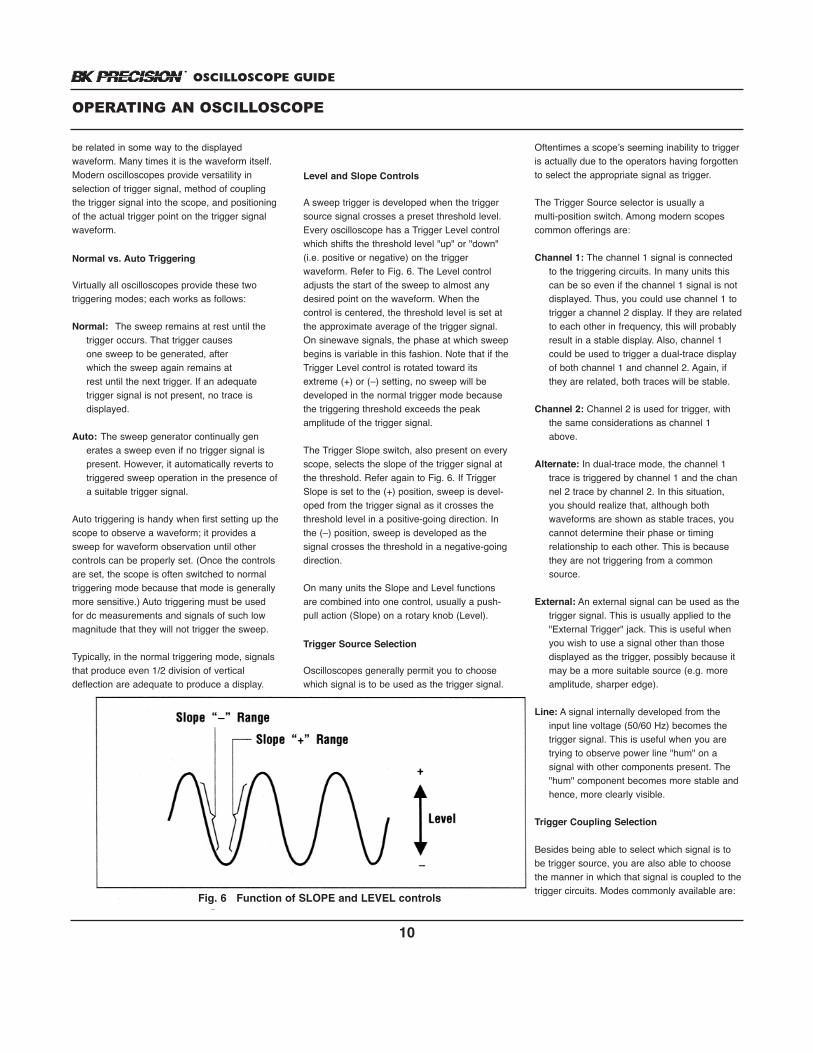
Level and Slope Controls

A sweep trigger is developed when the triggersource signal crosses a preset threshold level.Every oscilloscope has a Trigger Level controlwhich shifts the threshold level "up" or "down"(i.e. positive or negative) on the trigger waveform. Refer to Fig. 6. The Level controladjusts the start of the sweep to almost anydesired point on the waveform. When the control is centered, the threshold level is set atthe approximate average of the trigger signal.On sinewave signals, the phase at which sweepbegins is variable in this fashion. Note that if theTrigger Level control is rotated toward itsextreme (+) or (–) setting, no sweep will bedeveloped in the normal trigger mode becausethe triggering threshold exceeds the peak amplitude of the trigger signal.

The Trigger Slope switch, also present on everyscope, selects the slope of the trigger signal atthe threshold. Refer again to Fig. 6. If TriggerSlope is set to the (+) position, sweep is devel-oped from the trigger signal as it crosses thethreshold level in a positive-going direction. Inthe (–) position, sweep is developed as the signal crosses the threshold in a negative-goingdirection.

On many units the Slope and Level functionsare combined into one control, usually a push-pull action (Slope) on a rotary knob (Level).

Trigger Source Selection

Oscilloscopes generally permit you to choosewhich signal is to be used as the trigger signal.

Oftentimes a scope’s seeming inability to triggeris actually due to the operators having forgottento select the appropriate signal as trigger.

The Trigger Source selector is usually a multi-position switch. Among modern scopescommon offerings are:

Channel 1: The channel 1 signal is connected to the triggering circuits. In many units this can be so even if the channel 1 signal is not displayed. Thus, you could use channel 1 to trigger a channel 2 display. If they are relatedto each other in frequency, this will probably result in a stable display. Also, channel 1 could be used to trigger a dual-trace display of both channel 1 and channel 2. Again, if they are related, both traces will be stable.

Channel 2: Channel 2 is used for trigger, with the same considerations as channel 1 above.

Alternate: In dual-trace mode, the channel 1 trace is triggered by channel 1 and the channel 2 trace by channel 2. In this situation, you should realize that, although both waveforms are shown as stable traces, you cannot determine their phase or timing relationship to each other. This is because they are not triggering from a common source.

External: An external signal can be used as thetrigger signal. This is usually applied to the "External Trigger" jack. This is useful when you wish to use a signal other than those displayed as the trigger, possibly because it may be a more suitable source (e.g. more amplitude, sharper edge).

Line: A signal internally developed from the input line voltage (50/60 Hz) becomes the trigger signal. This is useful when you are trying to observe power line "hum" on a signal with other components present. The "hum" component becomes more stable and hence, more clearly visible.

Trigger Coupling Selection

Besides being able to select which signal is tobe trigger source, you are also able to choosethe manner in which that signal is coupled to thetrigger circuits. Modes commonly available are:


Fig. 6 Function of SLOPE and LEVEL controls

OSCILLOSCOPE GUIDE

11

AC: This is used for viewing most types of waveforms. The trigger signal is capacitively coupled (dc component blocked) and may beused for all signals from below 30 Hz (depending on the unit) to the top frequency of the particular scope.

DC: Couples both the ac and dc component of the trigger signal. This is useful for viewing signals with frequency lower than the cutoff of the "AC" position above, or when you need to include the dc component for proper stabilization of the signal.

TV-H: Used for viewing horizontal sync pulses incomposite video waveforms. A high-pass filter is employed, which couples through only higher-frequency components such as horizontal sync pulses. This position can alsobe used as a general high-pass (low-frequency reject) position, and as such is sometimes labeled "HF".

TV-V: Used for viewing vertical sync pulses in composite video waveforms. A low-pass filteris employed, which couples through only lower-frequency components such as verticalsync pulses. This position can also be used as a general low-pass (high-frequency reject)position, and as such is sometimes labeled "LF".

Video: On some scopes, this general setting is provided instead of the two previous ones. Coupling is automatically switched between horizontal or vertical sync pulses depending on the setting of the main time base.

Vertical and Horizontal Magnifiers

Most scopes permit magnification of the on-screen waveform in both the vertical and horizontal direction.

Vertical magnifiers are usually implemented as apush-pull action on the Variable control for eachvertical attenuator. Generally a factor of X5, thismagnification can also be thought of as extending the sensitivity of the unit by one ortwo ranges. For example, if a scope has a minimum vertical attenuator setting of 5 mV/division, the X5 multiplier can provide twoextra ranges: 2 mV/division (on the regular 10mV/division setting) and 1 mV/division (on the

regular 5 mV/division setting).

With this increase in ranges, however, come twoperformance degradations. First, the bandwidthof the scope is reduced when the magnifier isactive. The reduction may he drastic; a 60 MHzunit may be limited to 10 MHz in this mode. (Fora discussion of the bandwidth concept, see the"Bandwidth" section of this chapter. ) Secondly,using the magnifier on the most sensitive settings results in increased noise on the waveform. The trace appears thicker and out-of-focus.

Horizontal magnification is usually achievedthrough a push-pull action on either the VariableTime Base control or the Horizontal Positioncontrol. Magnification factor is usually X 10. Thisfeature is helpful in viewing a portion of a waveform that might disappear off the right ofthe screen if the Time Base setting is increased.Even though the waveform is magnified, rotatingthe Horizontal Position control can still enableyou to observe every portion of it.

The Add and Invert Functions

A very common feature on modern oscilloscopes is the Add mode, which permitsthe channel 1 and channel 2 signals to be algebraically combined and displayed as onetrace. This feature is particularly useful whenused in conjunction with the "Invert" function.Invert takes one of the input channels andreverses its polarity on the display. For example,the highs of a sine wave are shown as lows,and vice versa. Any dc offset is also inverted(i.e. a positive dc offset becomes a negativeone), assuming that the scope is set for dc coupling.

In effect, when an uninverted channel is addedto an inverted one, the result is the algebraic difference. This is handy for differential measurements (when you wish to observe a signal not referenced to ground) and eliminationof undesired signal components. Both uses arediscussed in the "Applications" chapter of thismanual.

The Add function is usually implemented on thesame control that selects single-trace or dual-trace mode, i.e. the Vertical Mode control.The Invert function may be implemented onchannel 1 or channel 2, depending on the

particular scope, and may be a Vertical Modecontrol, a secondary function of the Variableattenuator, or a separate switch.

X-Y Operation

X-Y operation permits the oscilloscope to perform many measurements not possible withconventional sweep operation. The CRT displaybecomes an electronic graph of two instanta-neous voltages. One voltage deflects the beamvertically (Y), and the other deflects it horizontal-ly (X). The sweep aspects of the scope are disabled. Thus, with no signals connected, thedisplay is merely a dot.

The signals being applied may be two voltages,such as stereoscope display of stereo signaloutputs. However, the X-Y mode can be used tograph almost any dynamic characteristic if atransducer is used to change the characteristic(frequency, temperature, velocity, etc.) into avoltage. One common application is frequencyresponse measurements, where the Y axis corresponds to signal amplitude and the X axisto frequency.

The controls used to implement X-Y mode varyamong different scopes. However, the generalprocedure for using it is as follows:

1. Locate the switch that enables X-Y mode. This may be a separate switch, or the last position of the Time Base selector. On scopes with delayed sweep capability, it is usually one of the Sweep Mode selections. Turn on the X-Y mode. Make sure the trace intensity is not set too high; a bright stationary dot in one spot on the screen can be damaging if left there for a long time.

2. The channel 1 and channel 2 inputs now become X and Y inputs, though not necessarily in that order. Apply the desired signals to these channels.

3. The vertical attenuators now become the X and Y attenuators, i.e. one controls the height of the waveform, and the other its width. The Variable attenuator controls function similarly.

4. Positioning of the X-Y waveform is as follows:


OSCILLOSCOPE GUIDE

12

a. Generally, the Vertical Position control of whichever channel is the Y-axis becomes

the vertical positioning control for X-Ydisplays.

b. Horizontal positioning is accomplished by either the vertical control for the other channel, or the Horizontal Position controlfor the scope.

The "Applications" chapter discusses two common uses of X-Y mode, phase measurements and frequency response measurements.

Bandwidth

Bandwidth, or frequency response, is one of themost important characteristics of an oscillo-scope. It is often the determining factor in pre-ferring one unit over another.

By convention, bandwidth, which is measured inMHz, is the frequency at which signal amplitude"rolls off" by 3 dB from its value at 1 kHz. Forexample, assume that a 1 kHz signal producesa waveform six divisions high on a givenVolts/Div setting. If that signal is increased infrequency (but input amplitude is kept constant),the frequency at which the display is reduced to4.24 divisions (–3 dB, or 70.7%) is the bandwidth of the scope.

Bandwidth is important because it dictates thehighest frequency at which accurate measurements can be made with a given oscilloscope. As might be expected, the scopebuyer pays more for higher bandwidth. The

range of applications and measurements goesup as the bandwidth does, and the availability ofadvanced features also increases. Basic oscilloscopes such as those discussed so farare generally 20 MHz or 30 MHz units. Higherbandwidths include 40 MHz, 60 MHz, 100 MHz,and beyond. The features discussed in the nextsection usually imply a minimum bandwidth of40 MHz.

Using an Oscilloscope with 1 millivoltSensitivity

Many oscilloscopes have a X5 MAG (5 timesmagnification of the vertical input signal) feature.With X5 magnification, the 10 mV/div attenuatorsetting becomes 2 mV/div sensitivity, and the 5mV/div attenuator setting becomes 1 mV/divsensitivity. At these high sensitivity settings, special care must be taken for reliable low levelmeasurements. Keep the following points inmind when measuring very low level signals.

• Placement of the ground clip may become critical if the signal ground circuitry carries appreciable current. Voltage differences of several millivolts are common from one side of a chassis to another. Attach the ground clip to a ground point nearest the point of signal measurement (the probe tip). This usually gives the smallest error. You may need to move the ground clip as you move the probe to other points of measurement.

• It may be difficult to eliminate the pickup of stray 60 Hz signals, especially in high impedance circuits. Be sure to use shielded

test cables. If necessary, shield the area around the probe tip.Wideband measurements become more difficult at 1 mV/div and 2 mV/div because of the inherentthermal noise of electronic components. The trace may appear "fuzzy" or wide and out of focus.

• Noise that appears as peaks or spikes may be caused by electromagnetic pickup of external interference, such as automotive ignition, computer clock pulses, etc. Such noise may also cause erratic triggering. If possible, shield the unit under test from external interference.

• Radio interference may be picked up in strong RF signal areas, such as a nearby AM broadcast station, CB radios, or other transmitting devices. Unshielded probes and test cables can act as antennas to magnify this type of interference.

• Use the lowest sensitivity possible for the measurement. Do not use 1 mV/div sensitivity if the measurement can be made at 5 mV/div sensitivity. Perhaps the probe can be switched to X1 instead of using X5 MAG, however, be aware that the probe’s bandwidth is sharply reduced at X1 and its input impedance is much lower.

• Thermal drift may be apparent at high sensitivity if the test connections are across a semi-conductor junction or two dissimilar metals. The trace may drift as the junction temperature changes.



This section discusses advanced features generally found on higher-bandwidth oscilloscopes, such as delayed sweep, variableholdoff, etc. However, B+K Precision offers adeluxe 30 MHz oscilloscope with many of theadvanced features described here, includingdelayed sweep, component test, Y-axis output,and Z-axis input. This scope is Model 2125A.

Delayed Sweep

The delayed sweep feature permits the operatorto magnify a portion of the trace for closerexamination. While this can be done by usingthe horizontal magnifier as mentioned

previously, delayed sweep provides higherorders of magnification, many more degrees ofmagnification, and the means to observe boththe magnified and original waveforms simultaneously.

The feature is called "delayed sweep" becausethe magnification is achieved by delaying thebeginning of the trace for a period determinedby the operator. After this delay, the sweep thenruns at a speed which the operator sets via asecond Time Base control, separate from themain Time Base. By adjusting both the delaytime and the sweep speed, the operator variesthe position and the width of the magnified

portion.

The delayed sweep (often referred to as the Bsweep) begins immediately after the delay period selected by the operator is over.Adjustment range of the delay time is "continuous".

Note:

To obtain meaningful results with delayedsweep, the delayed sweep must be set to afaster sweep speed than the main sweep. Thismakes sense, since we are magnifying a portionof the original waveform.

OSCILLOSCOPE GUIDE

13

or in-circuit on a non-powered chassis. The displayed pattern (signature) is a dynamic plotof the impedance of the component with a sinewave signal applied. This test technique is veryeffective at locating defective components. Thepreferred method of testing is to use patternsfrom a known-good chassis for reference.Shorted, open, and leaky components producepatterns very dissimilar from reference patterns.Good components produce patterns identical orvery similar to the reference patterns. Fig. 9shows some typical patterns using componenttest.

Other Advanced Features

Y-Axis OutputThis feature allows a sample of the vertical signal (usually channel 2, but may be channel 1on some oscilloscopes) to be used externally.The output signal is buffered from a low impedance source, usually 50 ohms. The amplitude of the Y-axis output is usually 50 millivolts per division of the vertical deflectionseen on the screen of the CRT when terminatedinto 50 ohms. When unterminated (or terminated into a high impedance), the output is 100 mV/div. The Y-axis output allowsthe oscilloscope to be used as a wideband preamplifier. One typical application is to amplifya low level signal adequately to drive a frequency counter. A 10 mV peak-to-peak signal(about 3.6 mV rms) is not adequate to drivemost frequency counters, however, it is enoughto give two vertical divisions amplitude on an

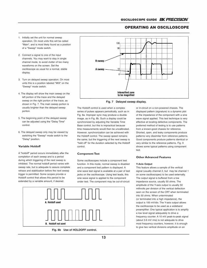
The Holdoff control is used when a complexseries of pulses appears periodically, such as inFig. 8a. Improper sync may produce a doubleimage, as in Fig. 8b. Such a display could besynchronized by adjusting the Variable TimeBase control, but this is impractical becausetime measurements would then be uncalibrated.However, synchronization can be achieved withthe Holdoff control. The sweep speed remainsthe same, but the triggering of the next sweep is"held off" for the duration selected by the Holdoffcontrol.

Component Test

Some oscilloscopes include a component testfunction. In this mode, normal sweep is disabledand a component test pattern is displayed. Asine wave test signal is available at a pair of testjacks on the oscilloscope. Using test leads, thissine wave signal is applied to the componentunder test. The component may be out-of-circuit

1. Initially set the unit for normal sweep operation. On most units this will be called "Main", and is most likely found as a positionof a "Sweep" mode switch.

2. Connect a signal to one of the input channels. You may want to stay in single channel mode, to avoid clutter of too many waveforms on the screen. Set the oscilloscope as usual for a normal, stable display.

3. Turn on delayed sweep operation. On most units this is a position labeled "MIX" on the "Sweep" mode switch.

4. The display will show the main sweep on the left portion of the trace and the delayed sweep on the right portion of the trace, as shown in Fig. 7. The main sweep portion is usually brighter than the delayed sweep portion.

5. The beginning point of the delayed sweep can be adjusted using the "Delay Time" control.

6. The delayed sweep only may be viewed by switching the "Sweep" mode switch to the "Delay" position.

Variable Holdoff

A "holdoff" period occurs immediately after thecompletion of each sweep and is a period during which triggering of the next sweep isinhibited. The normal holdoff period varies withsweep rate, but is adequate to assure completeretrace and stabilization before the next sweeptrigger is permitted. Some scopes provide aHoldoff control that allows this period to beextended by a variable amount, if desired.


Fig. 7 Delayed sweep display.

Fig. 8b Use of HOLDOFF control.

OSCILLOSCOPE GUIDE

14

oscilloscope set at 5 mV/div sensitivity. With twodivisions deflection on the CRT, the output ofthe Y-axis output (terminated into 1 megohminput impedance of most counters) is 200 millivolts peak-to-peak or 71 millivolts rms. Thisis plenty to drive the frequency counter solidly.

Z-Axis InputThis feature is sometimes called intensity modulation. When a signal is applied to therear-panel Z-Axis input jack, the electron beam(which produces the scope display) varies inintensity according to the amplitude of that input.Thus, the display can be intensity modulated ina manner similar to a video or television display.Usually, the front panel Intensity control can beadjusted so that TTL levels at the Z-Axis jackturn the beam on and off completely. The polarity of the modulation depends on the particular model of scope. Some displays growbrighter with a more positive voltage; othersrequire a more negative voltage for a brighterdisplay.

Beam FinderThis convenience feature helps you to find atrace that may be off the area of the screen.Beam Finder compresses the trace and "pulls" itinto the CRT area, so that you may know inwhich direction the trace is off screen, Don’tkeep this momentary function on for too long,however; it also puts the trace at full intensity tohelp you locate it..

Bandwidth LimiterOn higher-frequency scopes, this switch allowsthe bandwidth to be scaled down. For example,a 100 MHz unit might offer a limiter that reducesit to 20 MHz. This feature is useful for filteringout higher-frequency noise, such as radio frequency interference, when using the scopefor lower-frequency measurements.

Scale IlluminationThis is a control, placed near the scope display,which causes the graticule to be illuminated forvisibility in dark environments. This is usuallydone with small light bulbs placed around theperimeter of the display. The control varies theintensity of the illumination. The graticule iscomposed of a reflective substance that evensout the illumination over the total area of thegrid

Description

The digital storage oscilloscope, or DSO, is arecent major development in the oscilloscopefield. Instead of merely displaying a waveformon the CRT as it occurs, as does a standardanalog oscilloscope, the DSO digitizes theincoming signal, stores it in memory, then continuously displays the contents of the memory on the screen. This enables the operator to capture and view one-time events,including activity immediately before the eventitself (pre-trigger capture). DSOs are also excellent for displaying slow events that are difficult or impossible to view on standard analog oscilloscopes. DSOs can also storerepetitive waveforms in memory, as well as one-time or slow waveforms, and transfer them to aplotter for future reference.

Although DSOs vary widely in features andoperation, most DSOs include the basic featuresdescribed in the following discussion, which isbased on B+K Precision Model 2522B. TheModel 2522B is a "hybrid" unit that can operatein conventional analog mode or in digital storagemode. The hybrid approach is often an advantage over full digital models in simplifyingsetup. The hybrid models can be adjusted in thefamiliar analog mode, then switched to digitalstorage operation for the actual waveform capture.

Digitizing One-time Events

One of the most powerful features of a digitalstorage oscilloscope is its ability to capture one-time events. To do this, single-sweep operationis employed, using the Single and Reset (orArm) button. When the Reset button is pressed,it readies the digital storage circuit to receive atrigger signal—presumably the event to be captured or some other time-related occurrence.When the event arrives, it is stored in memoryand displayed.

Capture of one-time events is an ideal use for ahybrid DSO. The triggering adjustments can bemade in analog mode, and then the actual cap-ture done in digital. The procedure is as follows:

1. Set the scope to analog mode. Set the Trigger Level control for normal (not auto) triggering, and adjust the level so that the unit

triggers on the event to be captured. This usually involves making the event occur a few times with the scope in analog mode. Using normal triggering is important because even though the event may be too brief to readily observe in analog mode, it will cause one sweep to cross the screen in normal triggering mode. This is helpful in getting the Trigger Level set correctly.

2. Press the Storage switch to enter the storagemode.

3. Press the Single button, then the Reset (or Arm) button. The Ready indicator (or Armed indicator) lights while waiting for the trigger signal and goes off when the trigger ofthe one-time event occurs.

4. The one-time event that has been captured inmemory is displayed continuously until Reset is pressed again to capture another one-time event or until the mode is changed.

Pre-trigger and Post-trigger View

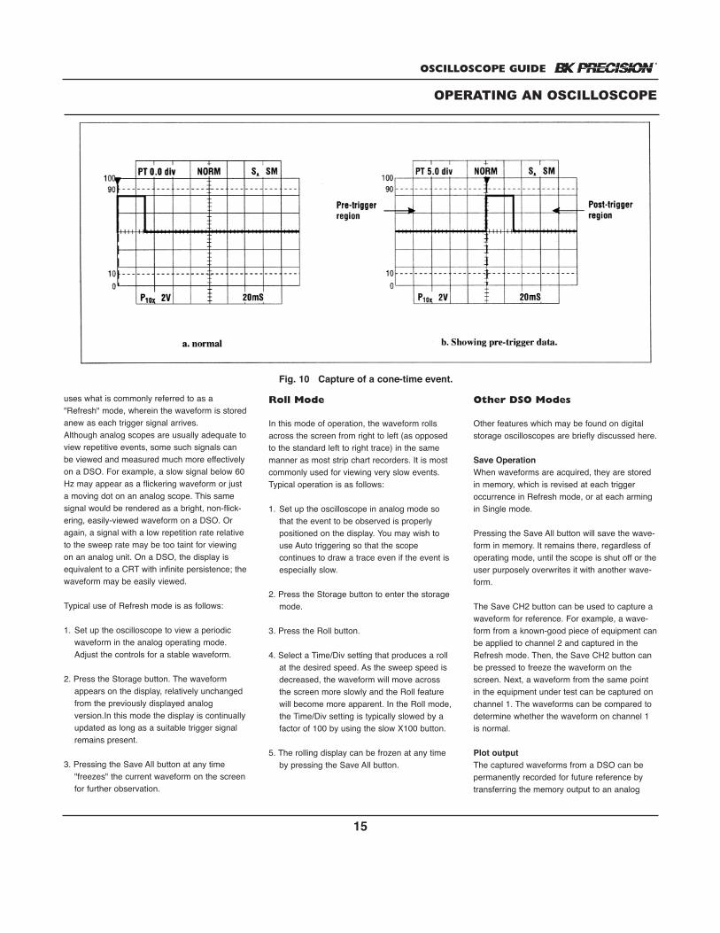
One of the big advantages of a DSO is its abilityto view occurrences before the trigger, or pre-trigger view, as well as occurrences after thetrigger, or post-trigger view. For example, notonly can a voltage spike be observed, but perhaps the activity that caused it. In a conventional analog oscilloscope, the sweepbegins at the trigger. Thus, only post-triggerevents can be viewed. In DSOs, waveformrecording does not begin with the occurrence ofa trigger, it is continuous. Rather, the triggerdetermines where the waveform recordingstops. The operator can set the trigger to occurat the beginning of the memory (0% pre-trigger),at the middle of the memory (50% pre-trigger),or at other points in the memory (25% and 75%pre-trigger with Model 2522B). Fig. 10a shows awaveform with 0% pre-trigger, and Fig. 10bshows the same waveform with 50% pre-trigger.Note that in Fig. 10b, observance of the timeperiod immediately before the trigger is possible.

Digitizing Repetitive Events

Though the capture of one-time events is probably the most powerful aspect of a DSO,many units can also digitize conventional repetitive waveforms, such as those observedon a standard analog scope. To do this, a DSO



OSCILLOSCOPE GUIDE

15

uses what is commonly referred to as a"Refresh" mode, wherein the waveform is storedanew as each trigger signal arrives.Although analog scopes are usually adequate toview repetitive events, some such signals canbe viewed and measured much more effectivelyon a DSO. For example, a slow signal below 60Hz may appear as a flickering waveform or justa moving dot on an analog scope. This samesignal would be rendered as a bright, non-flick-ering, easily-viewed waveform on a DSO. Oragain, a signal with a low repetition rate relativeto the sweep rate may be too taint for viewingon an analog unit. On a DSO, the display isequivalent to a CRT with infinite persistence; thewaveform may be easily viewed.

Typical use of Refresh mode is as follows:

1. Set up the oscilloscope to view a periodic waveform in the analog operating mode. Adjust the controls for a stable waveform.

2. Press the Storage button. The waveform appears on the display, relatively unchanged from the previously displayed analog version.In this mode the display is continuallyupdated as long as a suitable trigger signal remains present.

3. Pressing the Save All button at any time "freezes" the current waveform on the screenfor further observation.

Roll Mode

In this mode of operation, the waveform rollsacross the screen from right to left (as opposedto the standard left to right trace) in the samemanner as most strip chart recorders. It is mostcommonly used for viewing very slow events.Typical operation is as follows:

1. Set up the oscilloscope in analog mode so that the event to be observed is properly positioned on the display. You may wish to use Auto triggering so that the scope continues to draw a trace even if the event is especially slow.

2. Press the Storage button to enter the storage mode.

3. Press the Roll button.

4. Select a Time/Div setting that produces a roll at the desired speed. As the sweep speed is decreased, the waveform will move across the screen more slowly and the Roll feature will become more apparent. In the Roll mode,the Time/Div setting is typically slowed by a factor of 100 by using the slow X100 button.

5. The rolling display can be frozen at any time by pressing the Save All button.

Other DSO Modes

Other features which may be found on digitalstorage oscilloscopes are briefly discussed here.

Save OperationWhen waveforms are acquired, they are storedin memory, which is revised at each triggeroccurrence in Refresh mode, or at each armingin Single mode.

Pressing the Save All button will save the wave-form in memory. It remains there, regardless ofoperating mode, until the scope is shut off or theuser purposely overwrites it with another wave-form.

The Save CH2 button can be used to capture awaveform for reference. For example, a wave-form from a known-good piece of equipment canbe applied to channel 2 and captured in theRefresh mode. Then, the Save CH2 button canbe pressed to freeze the waveform on thescreen. Next, a waveform from the same pointin the equipment under test can be captured onchannel 1. The waveforms can be compared todetermine whether the waveform on channel 1is normal.

Plot outputThe captured waveforms from a DSO can bepermanently recorded for future reference bytransferring the memory output to an analog


Fig. 10 Capture of a cone-time event.

OSCILLOSCOPE GUIDE

16

plotter. First, the waveforms are frozen by pressing the Save All button. Then, an analogplotter can be connected to the channel 1 output, channel 2 output, and Pen Down outputjacks on the rear panel of the DSO. When interconnected, plotting can begin by pressingthe Plot button. The plot cycle is one screenfulon (pen down) and the next screenful off (pen up). The Pen Down indicator lights for theentire pen-down period of the plot cycle.

Unique Characteristics of DSOs

Digital storage oscilloscopes use a digital sampling technique to convert analog signals toa series of digital words that can be stored inmemory. Digital sampling has disadvantages aswell as advantages, and it is important to beaware of these unique characteristics of DSOs.Real Time Sampling and Aliasing

The DSO uses a technique called Real TimeSampling at sweep speeds slower than about20 ms/div. Real Time Sampling simply meansthat samples of the input signal are taken atequal spaces (e.g., every 0.25 mS when the 50mS/div range is selected). With Real TimeSampling, a phenomenon called "aliasing" canoccur when the input signal is not sampled oftenenough. This causes the digitized signal to

appear to be of a lower frequency than that ofthe input signal. Unless you have an idea whatthe input signal is supposed to look like, you willusually be unaware that aliasing is occurring.

To see an example of aliasing, connect a 10kHz signal to a DSO, set the Time/Div setting to50 mS/div, and put the scope in Refresh mode.You should see about five divisions displayed.Now change the Time/Div setting to 20 mS/div,and slightly alter the frequency of the input signal. If you do this carefully, you should beable to obtain a display that shows just a fewcycles at this low sweep speed. If you calculatethe frequency now, it appears to be somethinglike 50 Hz or below, which is obviously incorrect.

This occurs because the DSO is taking samplestoo slowly to accurately render the waveform onthe CRT, possibly one sample per cycle of theinput signal. If the input frequency is set justright, the samples come at a slightly differentpoint on each cycle, resulting in a waveform thatappears to be valid but in fact is not.

Aliasing can occur whenever at least two samples per cycle are not taken (whenever theTime/Div setting is much too slow for the inputsignal). Whenever the frequency of the inputsignal is unknown, always begin with the fastest

sweep speed, or view the waveform in analogmode first.Viewing of one-time events poses no problemwith aliasing because aliasing can occur onlywith repetitive waveforms.

Equivalent Time SamplingOn sweep speeds of 10 mS/div or greater, manyDSOs use a sampling method known asEquivalent Time Sampling. This method permitsviewing of repetitive waveforms of frequencieshigher than the scope’s sampling rate. WhenEquivalent Time Sampling is active, one sampleis taken during each cycle. Of course, if that onesample is taken right at the trigger point on eachcycle, a flat trace would be produced. Therefore,it is necessary to take each sample further (intime) from the trigger point than the last sample.This incremental delay is determined by thesweep Time/Div setting. To construct a completewaveform on the screen, the scope must sam-ple as many cycles of the input signal as thereare bytes in its memory.

Only repetitive waveforms should be observedin this mode. Irregularities that are present onan otherwise repetitive waveform are not likelyto show up; with only one sample per cycle,glitches and other irregularities will most likelybe skipped over.


OSCILLOSCOPE GUIDE

17

BASIC ANALOG OSCILLOSCOPES

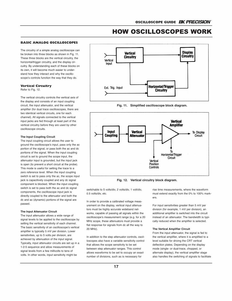
The circuitry of a simple analog oscilloscope canbe broken into three blocks as shown in Fig. 11.These three blocks are the vertical circuitry, thehorizontal/trigger circuitry, and the display cir-cuitry. By understanding each of these blocks onits own, it will become much easier to under-stand how they interact and why the oscillo-scope’s controls function the way that they do.

Vertical CircuitryRefer to Fig. 12.

The vertical circuitry controls the vertical axis ofthe display and consists of an input coupling circuit, the input attenuator, and the verticalamplifier (for dual trace oscilloscopes, there aretwo identical vertical circuits, one for each channel). All signals connected to the verticalinput jacks are fed through at least part of thevertical circuitry before they are used by otheroscilloscope circuits.

The Input Coupling CircuitThe input coupling circuit allows the user toground the oscilloscope’s input, pass only the acportion of the signal, or pass both the ac and dcportions of the signal. When the input couplingcircuit is set to ground the scope input, theattenuator input is grounded, but the input jackis open (to prevent a short circuit at the probe).This mode is useful for setting the trace to azero reference level. When the input couplingswitch is set to pass only the ac, the scope inputjack is capacitively coupled and any dc signalcomponent is blocked. When the input couplingswitch is set to pass both the ac and dc signalcomponents, the oscilloscope input jack isdirectly coupled to the attenuator and both thedc and ac (dynamic) portions of the signal arepassed.

The Input Attenuator CircuitThe input attenuator allows a wide range of signal levels to be applied to the oscilloscope bysetting the vertical sensitivity of each channel.The basic sensitivity of an oscilloscope’s verticalamplifier is typically 5 mV per division. Lowersensitivities, up to 5 volts per division, areachieved by attenuation of the input signal.Typically, input attenuator circuits are set up in a1-2-5 sequence and allow measurements of signal levels from a few millivolts to tens ofvolts. In other words, input sensitivity might be

switchable to 5 volts/div, 2 volts/div, 1 volt/div,0.5 volts/div, etc.

In order to provide a calibrated voltage meas-urement on the display, vertical input attenua-tors must be highly accurate wideband net-works, capable of passing all signals within theoscilloscope’s measurement range (e.g. for a 20MHz scope, these attenuators must provide aflat response for signals from dc all the way to20 MHz).

In addition to the step attenuator controls, oscil-loscopes also have a variable sensitivity controlthat allows the scope sensitivity to be setbetween step attenuator ranges. This controlallows waveforms to be set to occupy an exactnumber of divisions, such as is necessary for

rise time measurements, where the waveformmust extend exactly from the 0% to 100% mark-ers.

For input sensitivities greater than 5 mV perdivision (for example, 1 mV per division), anadditional amplifier is switched into the circuitinstead of an attenuator. The bandwidth is typi-cally reduced when the amplifier is selected.

The Vertical Amplifier CircuitFrom the input attenuator, the signal is fed tothe vertical amplifier, where it is amplified to alevel suitable for driving the CRT vertical deflection plates. Depending on the displaymode (single- or dual-trace, chopped, or alternate display), the vertical amplifier stagealso handles the switching of signals to facilitate

HOW OSCILLOSCOPES WORK

Fig. 11. Simplified oscilloscope block diagram.

Fig. 12. Vertical circuitry block diagram.

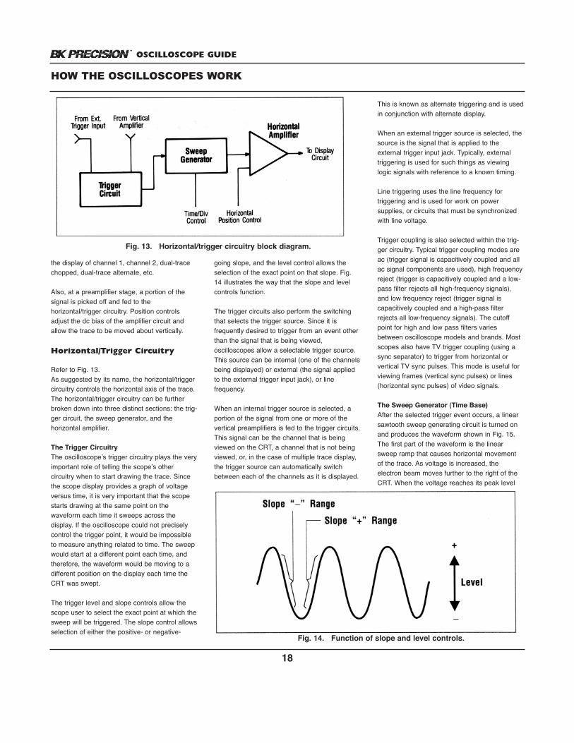
OSCILLOSCOPE GUIDE

18

the display of channel 1, channel 2, dual-tracechopped, dual-trace alternate, etc.

Also, at a preamplifier stage, a portion of thesignal is picked off and fed to the horizontal/trigger circuitry. Position controlsadjust the dc bias of the amplifier circuit andallow the trace to be moved about vertically.

Horizontal/Trigger Circuitry

Refer to Fig. 13.As suggested by its name, the horizontal/triggercircuitry controls the horizontal axis of the trace.The horizontal/trigger circuitry can be furtherbroken down into three distinct sections: the trig-ger circuit, the sweep generator, and the horizontal amplifier.

The Trigger CircuitryThe oscilloscope’s trigger circuitry plays the veryimportant role of telling the scope’s other circuitry when to start drawing the trace. Sincethe scope display provides a graph of voltageversus time, it is very important that the scopestarts drawing at the same point on the waveform each time it sweeps across the display. If the oscilloscope could not preciselycontrol the trigger point, it would be impossibleto measure anything related to time. The sweepwould start at a different point each time, andtherefore, the waveform would be moving to adifferent position on the display each time theCRT was swept.

The trigger level and slope controls allow thescope user to select the exact point at which thesweep will be triggered. The slope control allowsselection of either the positive- or negative-

going slope, and the level control allows theselection of the exact point on that slope. Fig.14 illustrates the way that the slope and levelcontrols function.

The trigger circuits also perform the switchingthat selects the trigger source. Since it is frequently desired to trigger from an event otherthan the signal that is being viewed, oscilloscopes allow a selectable trigger source.This source can be internal (one of the channelsbeing displayed) or external (the signal appliedto the external trigger input jack), or line frequency.

When an internal trigger source is selected, aportion of the signal from one or more of thevertical preamplifiers is fed to the trigger circuits.This signal can be the channel that is beingviewed on the CRT, a channel that is not beingviewed, or, in the case of multiple trace display,the trigger source can automatically switchbetween each of the channels as it is displayed.

This is known as alternate triggering and is usedin conjunction with alternate display.

When an external trigger source is selected, thesource is the signal that is applied to the external trigger input jack. Typically, externaltriggering is used for such things as viewinglogic signals with reference to a known timing.

Line triggering uses the line frequency for triggering and is used for work on power supplies, or circuits that must be synchronizedwith line voltage.

Trigger coupling is also selected within the trig-ger circuitry. Typical trigger coupling modes areac (trigger signal is capacitively coupled and allac signal components are used), high frequencyreject (trigger is capacitively coupled and a low-pass filter rejects all high-frequency signals),and low frequency reject (trigger signal is capacitively coupled and a high-pass filterrejects all low-frequency signals). The cutoffpoint for high and low pass filters variesbetween oscilloscope models and brands. Mostscopes also have TV trigger coupling (using async separator) to trigger from horizontal or vertical TV sync pulses. This mode is useful forviewing frames (vertical sync pulses) or lines(horizontal sync pulses) of video signals.

The Sweep Generator (Time Base)After the selected trigger event occurs, a linearsawtooth sweep generating circuit is turned onand produces the waveform shown in Fig. 15.The first part of the waveform is the linearsweep ramp that causes horizontal movementof the trace. As voltage is increased, the electron beam moves further to the right of theCRT. When the voltage reaches its peak level

HOW THE OSCILLOSCOPES WORK

Fig. 13. Horizontal/trigger circuitry block diagram.

Fig. 14. Function of slope and level controls.

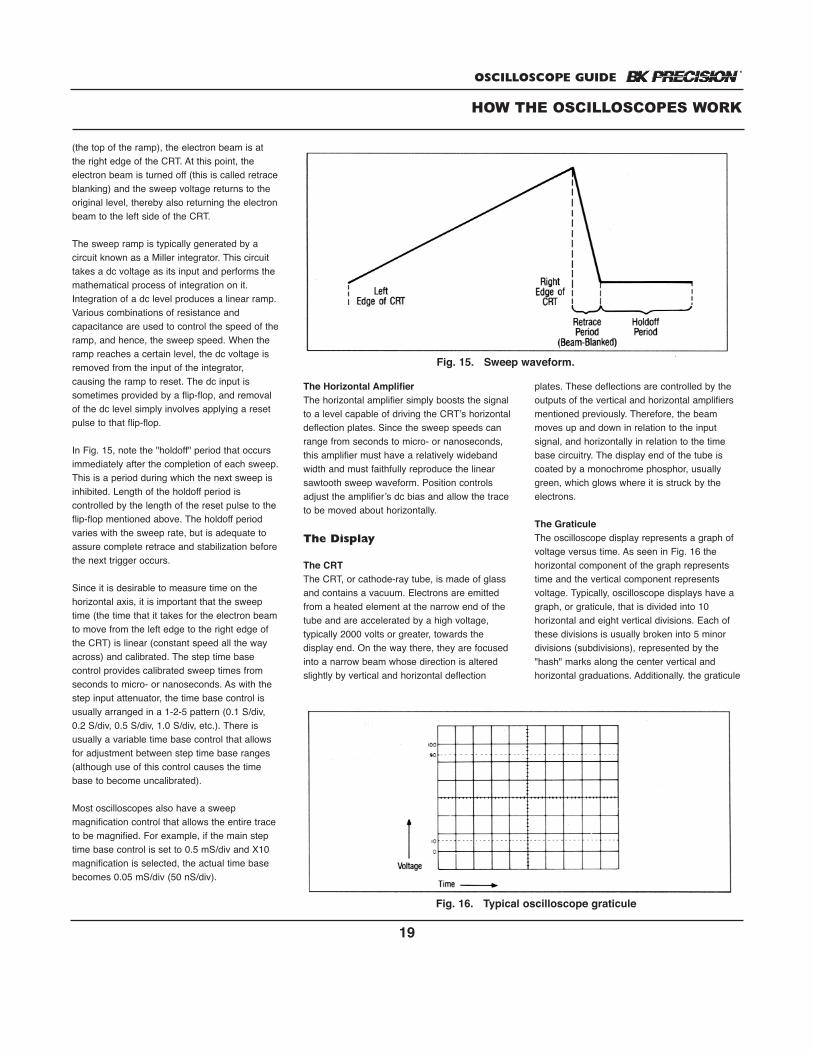
OSCILLOSCOPE GUIDE

19

(the top of the ramp), the electron beam is atthe right edge of the CRT. At this point, the electron beam is turned off (this is called retraceblanking) and the sweep voltage returns to theoriginal level, thereby also returning the electronbeam to the left side of the CRT.

The sweep ramp is typically generated by a circuit known as a Miller integrator. This circuittakes a dc voltage as its input and performs themathematical process of integration on it.Integration of a dc level produces a linear ramp.Various combinations of resistance and capacitance are used to control the speed of theramp, and hence, the sweep speed. When theramp reaches a certain level, the dc voltage isremoved from the input of the integrator, causing the ramp to reset. The dc input is sometimes provided by a flip-flop, and removalof the dc level simply involves applying a resetpulse to that flip-flop.

In Fig. 15, note the "holdoff" period that occursimmediately after the completion of each sweep.This is a period during which the next sweep isinhibited. Length of the holdoff period is controlled by the length of the reset pulse to theflip-flop mentioned above. The holdoff periodvaries with the sweep rate, but is adequate toassure complete retrace and stabilization beforethe next trigger occurs.

Since it is desirable to measure time on the horizontal axis, it is important that the sweeptime (the time that it takes for the electron beamto move from the left edge to the right edge ofthe CRT) is linear (constant speed all the wayacross) and calibrated. The step time base control provides calibrated sweep times fromseconds to micro- or nanoseconds. As with thestep input attenuator, the time base control isusually arranged in a 1-2-5 pattern (0.1 S/div,0.2 S/div, 0.5 S/div, 1.0 S/div, etc.). There isusually a variable time base control that allowsfor adjustment between step time base ranges(although use of this control causes the timebase to become uncalibrated).

Most oscilloscopes also have a sweep magnification control that allows the entire traceto be magnified. For example, if the main steptime base control is set to 0.5 mS/div and X10magnification is selected, the actual time basebecomes 0.05 mS/div (50 nS/div).

The Horizontal AmplifierThe horizontal amplifier simply boosts the signalto a level capable of driving the CRT’s horizontaldeflection plates. Since the sweep speeds canrange from seconds to micro- or nanoseconds,this amplifier must have a relatively widebandwidth and must faithfully reproduce the linearsawtooth sweep waveform. Position controlsadjust the amplifier’s dc bias and allow the traceto be moved about horizontally.

The Display

The CRTThe CRT, or cathode-ray tube, is made of glassand contains a vacuum. Electrons are emittedfrom a heated element at the narrow end of thetube and are accelerated by a high voltage, typically 2000 volts or greater, towards the display end. On the way there, they are focusedinto a narrow beam whose direction is alteredslightly by vertical and horizontal deflection

plates. These deflections are controlled by theoutputs of the vertical and horizontal amplifiersmentioned previously. Therefore, the beammoves up and down in relation to the input signal, and horizontally in relation to the timebase circuitry. The display end of the tube iscoated by a monochrome phosphor, usuallygreen, which glows where it is struck by theelectrons.

The GraticuleThe oscilloscope display represents a graph ofvoltage versus time. As seen in Fig. 16 the horizontal component of the graph representstime and the vertical component represents voltage. Typically, oscilloscope displays have agraph, or graticule, that is divided into 10 horizontal and eight vertical divisions. Each ofthese divisions is usually broken into 5 minordivisions (subdivisions), represented by the"hash" marks along the center vertical and horizontal graduations. Additionally. the graticule


Fig. 15. Sweep waveform.

Fig. 16. Typical oscilloscope graticule

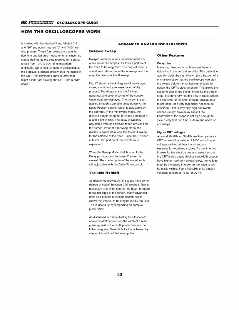
OSCILLOSCOPE GUIDE

20

is marked with two dashed lines, labeled "10"and "90" and points marked "0" and "100" arealso present. These four points are useful forrise time and fall time measurements, since risetime is defined as the time required for a signalto rise from 10% to 90% of its maximum amplitude. On almost all modern oscilloscopes,the graticule is etched directly onto the inside ofthe CRT. This eliminates parallax error thatmight occur from viewing the CRT from a slightangle.

Delayed Sweep

Delayed sweep is a very important feature ofmany advanced scopes. It allows a portion ofthe trace to be magnified. The original trace issometimes referred to as the A sweep, and themagnified trace as the B sweep.

Fig. 17 shows a block diagram of the delayedsweep circuit and a representation of theprocess. The trigger starts the A sweep generator and several cycles of the squarewave input are displayed. The trigger is alsoapplied through a variable delay network, theDelay Position control, which is adjustable bythe operator. In the Mix sweep mode, thedelayed trigger starts the B sweep generator ata later point in time. The delay is typicallyadjustable from one division to ten divisions onthe screen. When the B sweep starts, the display is switched to view the faster B sweepfor the balance of the trace. Since the B sweepis faster, that portion of the waveform is expanded.

When the Sweep Mode Switch is set to theDelay position, only the faster B sweep isviewed. The starting point of the waveform isstill adjustable with the Delay Time control.

Variable Holdoff

As mentioned previously, all scopes have somedegree of holdoff between CRT sweeps. This isnecessary to provide time for the beam to returnto the left edge of the screen. Many advancedunits also provide a variable holdoff, whichallows this interval to be lengthened by the user.This is useful for synchronizing on complexpulse trains.

As discussed in "Basic Analog Oscilloscopes"above, holdoff depends on the width of a resetpulse applied to the flip-flop, which drives theMiller integrator. Variable holdoff is achieved byvarying the width of that reset pulse.

Other Features

Delay LineMany high bandwidth oscilloscopes have adelay line in the vertical amplifier. This delay lineactually slows the signal down (by a fraction of amicrosecond) so that the oscilloscope can startthe sweep before the vertical signal starts todeflect the CRT’s electron beam. This allows thescope to display the signal, including the triggeredge. It is generally needed only in cases wherethe rise time (or fall time, if trigger occurs on afalling edge) of a very fast signal needs to beobserved. That is why only high bandwidthscopes usually have delay lines; if the bandwidth of the scope is not high enough toview a very fast rise time, a delay line offers noadvantage.

Higher CRT VoltagesA typical 20 MHz or 30 MHz oscilloscope has aCRT acceleration voltage of 2000 volts. Highervoltages deliver brighter traces and are essential for wideband scopes. As the time thatit takes for the electron beam to sweep acrossthe CRT is decreased (higher bandwidth scopeshave higher maximum sweep rates), the voltagemust be increased in order for the trace to stillbe easily visible. Some 100 MHz units employvoltages as high as 15 kV or 20 kV.



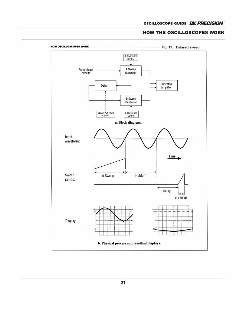
OSCILLOSCOPE GUIDE

21


Fig. 17. Delayed sweep.

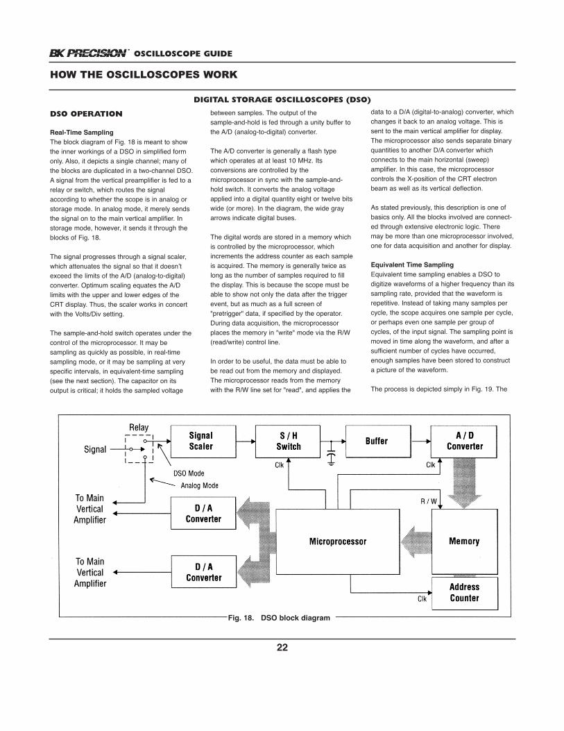
OSCILLOSCOPE GUIDE

22

DSO OPERATION

Real-Time SamplingThe block diagram of Fig. 18 is meant to showthe inner workings of a DSO in simplified formonly. Also, it depicts a single channel; many ofthe blocks are duplicated in a two-channel DSO.A signal from the vertical preamplifier is fed to arelay or switch, which routes the signal according to whether the scope is in analog orstorage mode. In analog mode, it merely sendsthe signal on to the main vertical amplifier. Instorage mode, however, it sends it through theblocks of Fig. 18.

The signal progresses through a signal scaler,which attenuates the signal so that it doesn’texceed the limits of the A/D (analog-to-digital)converter. Optimum scaling equates the A/D limits with the upper and lower edges of theCRT display. Thus, the scaler works in concertwith the Volts/Div setting.

The sample-and-hold switch operates under thecontrol of the microprocessor. It may be sampling as quickly as possible, in real-timesampling mode, or it may be sampling at veryspecific intervals, in equivalent-time sampling(see the next section). The capacitor on its output is critical; it holds the sampled voltage

between samples. The output of the sample-and-hold is fed through a unity buffer tothe A/D (analog-to-digital) converter.

The A/D converter is generally a flash typewhich operates at at least 10 MHz. Its conversions are controlled by the microprocessor in sync with the sample-and-hold switch. It converts the analog voltageapplied into a digital quantity eight or twelve bitswide (or more). In the diagram, the wide grayarrows indicate digital buses.

The digital words are stored in a memory whichis controlled by the microprocessor, which increments the address counter as each sampleis acquired. The memory is generally twice aslong as the number of samples required to fillthe display. This is because the scope must beable to show not only the data after the triggerevent, but as much as a full screen of "pretrigger" data, if specified by the operator.During data acquisition, the microprocessorplaces the memory in "write" mode via the R/W(read/write) control line.

In order to be useful, the data must be able tobe read out from the memory and displayed.The microprocessor reads from the memorywith the R/W line set for "read", and applies the

data to a D/A (digital-to-analog) converter, whichchanges it back to an analog voltage. This issent to the main vertical amplifier for display.The microprocessor also sends separate binaryquantities to another D/A converter which connects to the main horizontal (sweep) amplifier. In this case, the microprocessor controls the X-position of the CRT electronbeam as well as its vertical deflection.

As stated previously, this description is one ofbasics only. All the blocks involved are connect-ed through extensive electronic logic. Theremay be more than one microprocessor involved,one for data acquisition and another for display.

Equivalent Time SamplingEquivalent time sampling enables a DSO to digitize waveforms of a higher frequency than itssampling rate, provided that the waveform isrepetitive. Instead of taking many samples percycle, the scope acquires one sample per cycle,or perhaps even one sample per group ofcycles, of the input signal. The sampling point ismoved in time along the waveform, and after asufficient number of cycles have occurred,enough samples have been stored to constructa picture of the waveform.

The process is depicted simply in Fig. 19. The



Fig. 18. DSO block diagram

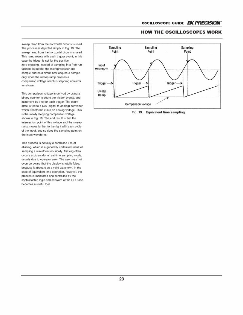
OSCILLOSCOPE GUIDE

23

sweep ramp from the horizontal circuits is used. The process is depicted simply in Fig. 19. Thesweep ramp from the horizontal circuits is used.This ramp resets with each trigger event; in thiscase the trigger is set for the positive zero-crossing. Instead of sampling in a free-runfashion as before, the microprocessor and sample-and-hold circuit now acquire a sampleonly when the sweep ramp crosses a comparison voltage which is stepping upwardsas shown.

This comparison voltage is derived by using abinary counter to count the trigger events, andincrement by one for each trigger. The countstate is fed to a D/A (digital-to-analog) converterwhich transforms it into an analog voltage. Thisis the slowly stepping comparison voltageshown in Fig. 19. The end result is that theintersection point of this voltage and the sweepramp moves further to the right with each cycleof the input, and so does the sampling point onthe input waveform.

This process is actually a controlled use ofaliasing, which is a generally undesired result ofsampling a waveform too slowly. Aliasing oftenoccurs accidentally in real-time sampling mode,usually due to operator error. The user may noteven be aware that the display is totally false,because it appears as a valid waveform. In thecase of equivalent-time operation, however, theprocess is monitored and controlled by thesophisticated logic and software of the DSO andbecomes a useful tool.


Fig. 19. Equivalent time sampling.

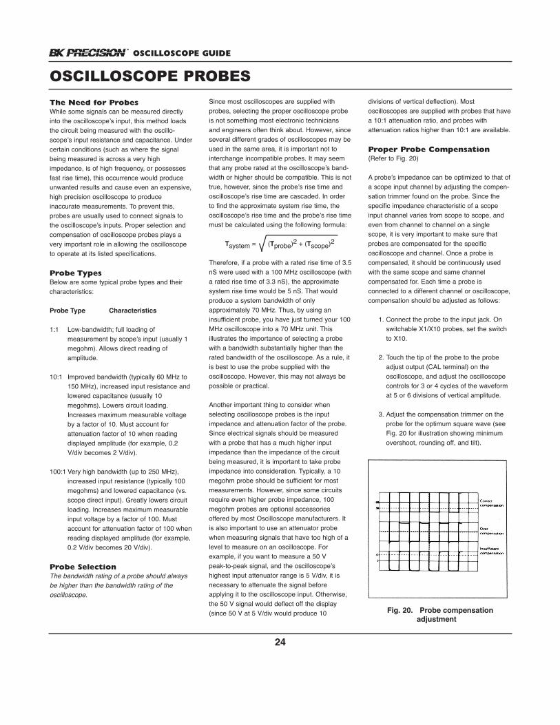
OSCILLOSCOPE GUIDE

24

The Need for ProbesWhile some signals can be measured directlyinto the oscilloscope’s input, this method loadsthe circuit being measured with the oscillo-scope’s input resistance and capacitance. Undercertain conditions (such as where the signalbeing measured is across a very high impedance, is of high frequency, or possessesfast rise time), this occurrence would produceunwanted results and cause even an expensive,high precision oscilloscope to produce inaccurate measurements. To prevent this,probes are usually used to connect signals tothe oscilloscope’s inputs. Proper selection andcompensation of oscilloscope probes plays avery important role in allowing the oscilloscopeto operate at its listed specifications.

Probe TypesBelow are some typical probe types and theircharacteristics:

Probe Type Characteristics

1:1 Low-bandwidth; full loading of measurement by scope’s input (usually 1 megohm). Allows direct reading of amplitude.

10:1 Improved bandwidth (typically 60 MHz to 150 MHz), increased input resistance and lowered capacitance (usually 10 megohms). Lowers circuit loading. Increases maximum measurable voltage by a factor of 10. Must account for attenuation factor of 10 when reading displayed amplitude (for example, 0.2 V/div becomes 2 V/div).

100:1 Very high bandwidth (up to 250 MHz), increased input resistance (typically 100 megohms) and lowered capacitance (vs. scope direct input). Greatly lowers circuit loading. Increases maximum measurable input voltage by a factor of 100. Must account for attenuation factor of 100 whenreading displayed amplitude (for example,0.2 V/div becomes 20 V/div).

Probe SelectionThe bandwidth rating of a probe should alwaysbe higher than the bandwidth rating of the oscilloscope.

Since most oscilloscopes are supplied withprobes, selecting the proper oscilloscope probeis not something most electronic techniciansand engineers often think about. However, sinceseveral different grades of oscilloscopes may beused in the same area, it is important not tointerchange incompatible probes. It may seemthat any probe rated at the oscilloscope’s band-width or higher should be compatible. This is nottrue, however, since the probe’s rise time andoscilloscope’s rise time are cascaded. In orderto find the approximate system rise time, theoscilloscope’s rise time and the probe’s rise timemust be calculated using the following formula:

Tsystem = (Tprobe)2 + (Tscope)2

Therefore, if a probe with a rated rise time of 3.5nS were used with a 100 MHz oscilloscope (witha rated rise time of 3.3 nS), the approximatesystem rise time would be 5 nS. That would produce a system bandwidth of only approximately 70 MHz. Thus, by using an insufficient probe, you have just turned your 100MHz oscilloscope into a 70 MHz unit. This illustrates the importance of selecting a probewith a bandwidth substantially higher than therated bandwidth of the oscilloscope. As a rule, itis best to use the probe supplied with the oscilloscope. However, this may not always bepossible or practical.

Another important thing to consider when selecting oscilloscope probes is the input impedance and attenuation factor of the probe.Since electrical signals should be measuredwith a probe that has a much higher inputimpedance than the impedance of the circuitbeing measured, it is important to take probeimpedance into consideration. Typically, a 10megohm probe should be sufficient for mostmeasurements. However, since some circuitsrequire even higher probe impedance, 100megohm probes are optional accessoriesoffered by most Oscilloscope manufacturers. Itis also important to use an attenuator probewhen measuring signals that have too high of alevel to measure on an oscilloscope. For example, if you want to measure a 50 V peak-to-peak signal, and the oscilloscope’shighest input attenuator range is 5 V/div, it isnecessary to attenuate the signal before applying it to the oscilloscope input. Otherwise,the 50 V signal would deflect off the display(since 50 V at 5 V/div would produce 10

divisions of vertical deflection). Most oscilloscopes are supplied with probes that havea 10:1 attenuation ratio, and probes with attenuation ratios higher than 10:1 are available.

Proper Probe Compensation(Refer to Fig. 20)

A probe’s impedance can be optimized to that ofa scope input channel by adjusting the compen-sation trimmer found on the probe. Since thespecific impedance characteristic of a scopeinput channel varies from scope to scope, andeven from channel to channel on a singlescope, it is very important to make sure thatprobes are compensated for the specific oscilloscope and channel. Once a probe is compensated, it should be continuously usedwith the same scope and same channel compensated for. Each time a probe is connected to a different channel or oscilloscope,compensation should be adjusted as follows:

1. Connect the probe to the input jack. On switchable X1/X10 probes, set the switch to X10.

2. Touch the tip of the probe to the probe adjust output (CAL terminal) on the oscilloscope, and adjust the oscilloscope controls for 3 or 4 cycles of the waveform at 5 or 6 divisions of vertical amplitude.

3. Adjust the compensation trimmer on the probe for the optimum square wave (see Fig. 20 for illustration showing minimum overshoot, rounding off, and tilt).

OSCILLOSCOPE PROBES

Fig. 20. Probe compensationadjustment

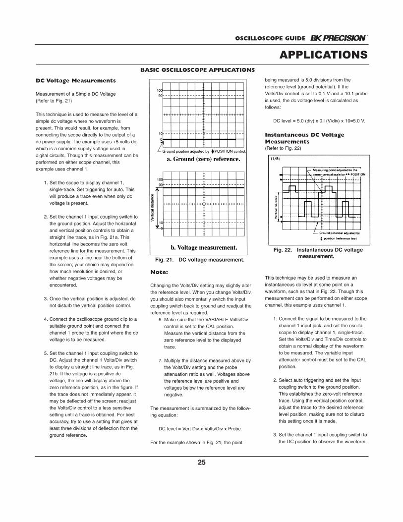
OSCILLOSCOPE GUIDE

25

DC Voltage Measurements

Measurement of a Simple DC Voltage(Refer to Fig. 21)

This technique is used to measure the level of asimple dc voltage where no waveform is present. This would result, for example, fromconnecting the scope directly to the output of adc power supply. The example uses +5 volts dc,which is a common supply voltage used in digital circuits. Though this measurement can beperformed on either scope channel, this example uses channel 1.

1. Set the scope to display channel 1, single-trace. Set triggering for auto. This will produce a trace even when only dc voltage is present.

2. Set the channel 1 input coupling switch tothe ground position. Adjust the horizontal and vertical position controls to obtain a straight line trace, as in Fig. 21a. This horizontal line becomes the zero volt reference line for the measurement. This example uses a line near the bottom of the screen; your choice may depend on how much resolution is desired, or whether negative voltages may be encountered.

3. Once the vertical position is adjusted, do not disturb the vertical position control.

4. Connect the oscilloscope ground clip to a suitable ground point and connect the channel 1 probe to the point where the dcvoltage is to be measured.

5. Set the channel 1 input coupling switch toDC. Adjust the channel 1 Volts/Div switch to display a straight line trace, as in Fig. 21b. If the voltage is a positive dc voltage, the line will display above the zero reference position, as in the figure. Ifthe trace does not immediately appear. it may be deflected off the screen; readjust the Volts/Div control to a less sensitive setting until a trace is obtained. For best accuracy, try to use a setting that gives atleast three divisions of deflection from theground reference.

Note:

Changing the Volts/Div setting may slightly alterthe reference level. When you change Volts/Div,you should also momentarily switch the inputcoupling switch back to ground and readjust thereference level as required.

6. Make sure that the VARIABLE Volts/Div control is set to the CAL position. Measure the vertical distance from the zero reference level to the displayed trace.

7. Multiply the distance measured above by the Volts/Div setting and the probe attenuation ratio as well. Voltages above the reference level are positive and voltages below the reference level are negative.

The measurement is summarized by the follow-ing equation:

DC level = Vert Div x Volts/Div x Probe.

For the example shown in Fig. 21, the point

being measured is 5.0 divisions from the reference level (ground potential). If theVolts/Div control is set to 0.1 V and a 10:1 probeis used, the dc voltage level is calculated as follows:

DC level = 5.0 (div) x 0.l (V/div) x 10=5.0 V.

Instantaneous DC VoltageMeasurements(Refer to Fig. 22)

This technique may be used to measure aninstantaneous dc level at some point on a waveform, such as that in Fig. 22. Though thismeasurement can be performed on either scopechannel, this example uses channel 1.

1. Connect the signal to be measured to thechannel 1 input jack, and set the oscilloscope to display channel 1, single-trace. Set the Volts/Div and Time/Div controls toobtain a normal display of the waveform to be measured. The variable input attenuator control must be set to the CALposition.

2. Select auto triggering and set the input coupling switch to the ground position. This establishes the zero-volt reference trace. Using the vertical position control, adjust the trace to the desired reference level position, making sure not to disturb this setting once it is made.

3. Set the channel 1 input coupling switch tothe DC position to observe the waveform,

APPLICATIONSBASIC OSCILLOSCOPE APPLICATIONS

Fig. 21. DC voltage measurement.

Fig. 22. Instantaneous DC voltagemeasurement.

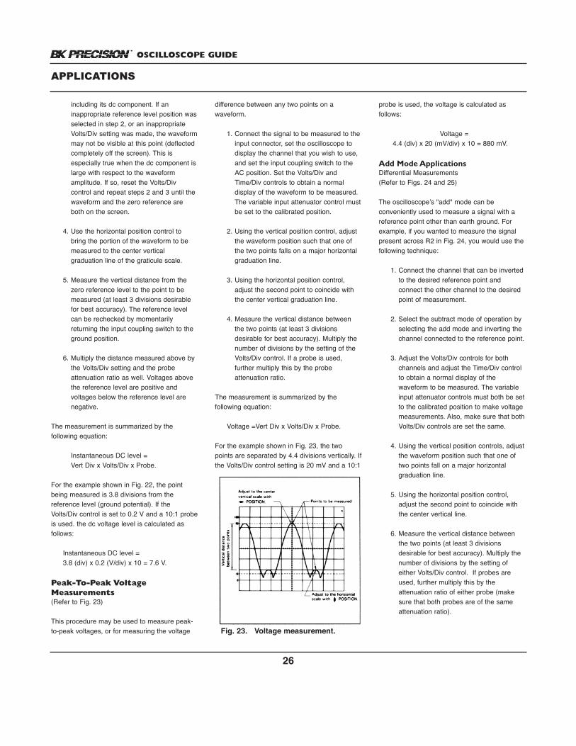
OSCILLOSCOPE GUIDE

26

including its dc component. If an inappropriate reference level position wasselected in step 2, or an inappropriate Volts/Div setting was made, the waveformmay not be visible at this point (deflected completely off the screen). This is especially true when the dc component islarge with respect to the waveform amplitude. If so, reset the Volts/Div control and repeat steps 2 and 3 until the waveform and the zero reference are both on the screen.

4. Use the horizontal position control to bring the portion of the waveform to be measured to the center vertical graduation line of the graticule scale.

5. Measure the vertical distance from the zero reference level to the point to be measured (at least 3 divisions desirable for best accuracy). The reference level can be rechecked by momentarily returning the input coupling switch to the ground position.

6. Multiply the distance measured above by the Volts/Div setting and the probe attenuation ratio as well. Voltages above the reference level are positive and voltages below the reference level are negative.

The measurement is summarized by the following equation:

Instantaneous DC level = Vert Div x Volts/Div x Probe.

For the example shown in Fig. 22, the pointbeing measured is 3.8 divisions from the reference level (ground potential). If theVolts/Div control is set to 0.2 V and a 10:1 probeis used. the dc voltage level is calculated as follows:

Instantaneous DC level = 3.8 (div) x 0.2 (V/div) x 10 = 7.6 V.

Peak-To-Peak VoltageMeasurements(Refer to Fig. 23)

This procedure may be used to measure peak-to-peak voltages, or for measuring the voltage

difference between any two points on a waveform.

1. Connect the signal to be measured to theinput connector, set the oscilloscope to display the channel that you wish to use, and set the input coupling switch to the AC position. Set the Volts/Div and Time/Div controls to obtain a normal display of the waveform to be measured. The variable input attenuator control mustbe set to the calibrated position.

2. Using the vertical position control, adjust the waveform position such that one of the two points falls on a major horizontal graduation line.

3. Using the horizontal position control, adjust the second point to coincide with the center vertical graduation line.

4. Measure the vertical distance between the two points (at least 3 divisions desirable for best accuracy). Multiply the number of divisions by the setting of the Volts/Div control. If a probe is used, further multiply this by the probe attenuation ratio.


Voltage =Vert Div x Volts/Div x Probe.

For the example shown in Fig. 23, the twopoints are separated by 4.4 divisions vertically. Ifthe Volts/Div control setting is 20 mV and a 10:1

probe is used, the voltage is calculated as follows:

Voltage =4.4 (div) x 20 (mV/div) x 10 = 880 mV.

Add Mode ApplicationsDifferential Measurements(Refer to Figs. 24 and 25)

The oscilloscope’s "add" mode can be conveniently used to measure a signal with areference point other than earth ground. For example, if you wanted to measure the signalpresent across R2 in Fig. 24, you would use thefollowing technique:

1. Connect the channel that can be inverted to the desired reference point and connect the other channel to the desired point of measurement.

2. Select the subtract mode of operation by selecting the add mode and inverting the channel connected to the reference point.

3. Adjust the Volts/Div controls for both channels and adjust the Time/Div control to obtain a normal display of the waveform to be measured. The variable input attenuator controls must both be setto the calibrated position to make voltage measurements. Also, make sure that bothVolts/Div controls are set the same.

4. Using the vertical position controls, adjustthe waveform position such that one of two points fall on a major horizontal graduation line.

5. Using the horizontal position control, adjust the second point to coincide with the center vertical line.

6. Measure the vertical distance between the two points (at least 3 divisions desirable for best accuracy). Multiply the number of divisions by the setting of either Volts/Div control. If probes are used, further multiply this by the attenuation ratio of either probe (make sure that both probes are of the same attenuation ratio).

APPLICATIONS

Fig. 23. Voltage measurement.

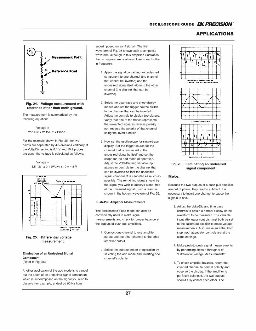
OSCILLOSCOPE GUIDE

27


Voltage = Vert Div x Volts/Div x Probe.

For the example shown in Fig. 25, the twopoints are separated by 4.5 divisions vertically. Ifthe Volts/Div setting is 0.1 V and 10:1 probesare used, the voltage is calculated as follows:

Voltage = 4.5 (div) x 0.1 (V/div) x 10 = 4.5 V

Elimination of an Undesired SignalComponent(Refer to Fig. 26)

Another application of the add mode is to cancelout the effect of an undesired signal componentwhich is superimposed on the signal you wish toobserve (for example, undesired 60 Hz hum

superimposed on an rf signal). The first waveform of Fig. 26 shows such a compositewaveform, although in this simplified illustrationthe two signals are relatively close to each otherin frequency.

1. Apply the signal containing an undesired component to one channel (the channel that cannot be inverted) and the undesired signal itself alone to the other channel (the channel that can be inverted).

2. Select the dual-trace and chop display modes and set the trigger source switch to the channel that can be inverted. Adjust the controls to display two signals. Verify that one of the traces represents the unwanted signal in reverse polarity. If not, reverse the polarity of that channel using the invert function.

3. Now set the oscilloscope for single-trace display: Set the trigger source for the channel that is connected to the undesired signal by itself and set the scope for the add mode of operation. Adjust the Volts/Div and variable input attenuator controls for the channel that can be inverted so that the undesired signal component is canceled as much aspossible. The remaining signal should be the signal you wish to observe alone, freeof the unwanted signal. Such a result is shown in the bottom waveform of Fig. 26.

Push-Pull Amplifier Measurements

The oscilloscope’s add mode can also be conveniently used to make signal measurements and check for proper balance atthe outputs of push-pull amplifiers.

1. Connect one channel to one amplifier output and the other channel to the other amplifier output.

2. Select the subtract mode of operation by selecting the add mode and inverting onechannel’s polarity.

Note:

Because the two outputs of a push-pull amplifierare out of phase, they tend to subtract. It is necessary to invert one channel to cause thesignals to add.

3. Adjust the Volts/Div and time base controls to obtain a normal display of the waveform to be measured. The variable input attenuator controls must both be setto the calibrated position to make voltage measurements. Also, make sure that bothstep input attenuator controls are at the same settings.

4. Make peak-to-peak signal measurements by performing steps 4 through 6 of "Differential Voltage Measurements".

5. To check amplifier balance, return the inverted channel to normal polarity and observe the display. If the amplifier is per fectly balanced, the two outputs should fully cancel each other. The

APPLICATIONS

Fig. 24. Voltage measurement withreference other than earth ground.

Fig. 25. Differential voltage measurement.

Fig. 26. Eliminating an undesiredsignal component

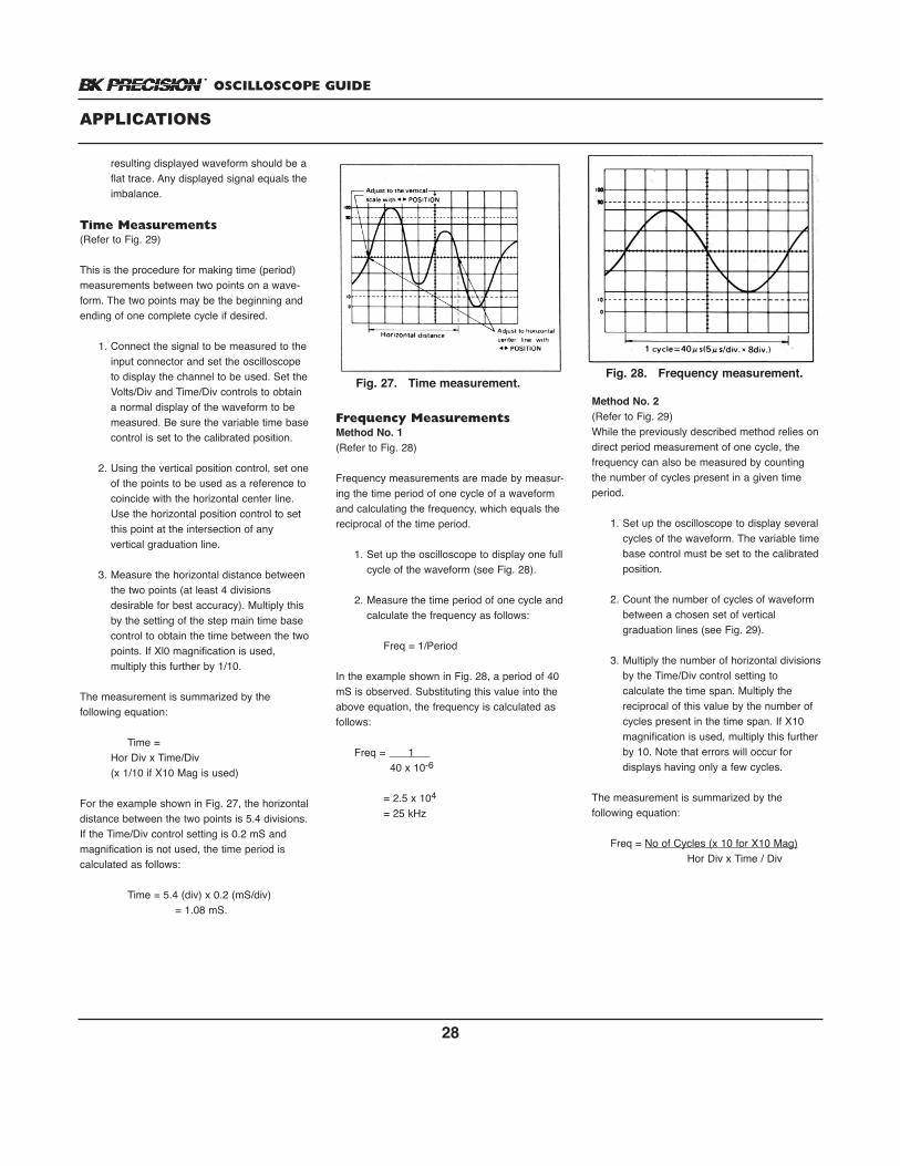
OSCILLOSCOPE GUIDE

28

resulting displayed waveform should be aflat trace. Any displayed signal equals theimbalance.

Time Measurements(Refer to Fig. 29)

This is the procedure for making time (period)measurements between two points on a wave-form. The two points may be the beginning andending of one complete cycle if desired.

1. Connect the signal to be measured to theinput connector and set the oscilloscope to display the channel to be used. Set theVolts/Div and Time/Div controls to obtain a normal display of the waveform to be measured. Be sure the variable time basecontrol is set to the calibrated position.

2. Using the vertical position control, set oneof the points to be used as a reference to coincide with the horizontal center line. Use the horizontal position control to set this point at the intersection of any vertical graduation line.

3. Measure the horizontal distance between the two points (at least 4 divisions desirable for best accuracy). Multiply this by the setting of the step main time base control to obtain the time between the twopoints. If Xl0 magnification is used, multiply this further by 1/10.


Time = Hor Div x Time/Div (x 1/10 if X10 Mag is used)

For the example shown in Fig. 27, the horizontaldistance between the two points is 5.4 divisions.If the Time/Div control setting is 0.2 mS andmagnification is not used, the time period is calculated as follows:

Time = 5.4 (div) x 0.2 (mS/div) = 1.08 mS.

Frequency MeasurementsMethod No. 1(Refer to Fig. 28)

Frequency measurements are made by measur-ing the time period of one cycle of a waveformand calculating the frequency, which equals thereciprocal of the time period.

1. Set up the oscilloscope to display one fullcycle of the waveform (see Fig. 28).

2. Measure the time period of one cycle andcalculate the frequency as follows:

Freq = 1/Period

In the example shown in Fig. 28, a period of 40mS is observed. Substituting this value into theabove equation, the frequency is calculated asfollows:

Freq = 1 40 x 10-6

= 2.5 x 104

= 25 kHz

Method No. 2(Refer to Fig. 29)While the previously described method relies ondirect period measurement of one cycle, the frequency can also be measured by countingthe number of cycles present in a given timeperiod.

1. Set up the oscilloscope to display severalcycles of the waveform. The variable timebase control must be set to the calibratedposition.

2. Count the number of cycles of waveform between a chosen set of vertical graduation lines (see Fig. 29).

3. Multiply the number of horizontal divisionsby the Time/Div control setting to calculate the time span. Multiply the reciprocal of this value by the number of cycles present in the time span. If X10 magnification is used, multiply this further by 10. Note that errors will occur for displays having only a few cycles.


Freq = No of Cycles (x 10 for X10 Mag)Hor Div x Time / Div

APPLICATIONS

Fig. 27. Time measurement.Fig. 28. Frequency measurement.

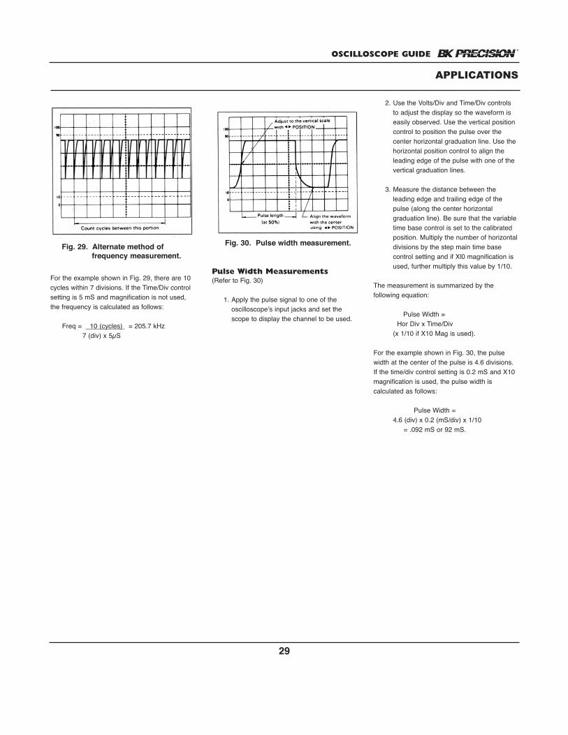
OSCILLOSCOPE GUIDE

29

For the example shown in Fig. 29, there are 10cycles within 7 divisions. If the Time/Div controlsetting is 5 mS and magnification is not used,the frequency is calculated as follows:

Freq = 10 (cycles) = 205.7 kHz7 (div) x 5µS

Pulse Width Measurements(Refer to Fig. 30)

1. Apply the pulse signal to one of the oscilloscope’s input jacks and set the scope to display the channel to be used.

2. Use the Volts/Div and Time/Div controls to adjust the display so the waveform is easily observed. Use the vertical position control to position the pulse over the center horizontal graduation line. Use the horizontal position control to align the leading edge of the pulse with one of the vertical graduation lines.

3. Measure the distance between the leading edge and trailing edge of the pulse (along the center horizontal graduation line). Be sure that the variabletime base control is set to the calibrated position. Multiply the number of horizontaldivisions by the step main time base control setting and if Xl0 magnification is used, further multiply this value by 1/10.


Pulse Width = Hor Div x Time/Div

(x 1/10 if X10 Mag is used).

For the example shown in Fig. 30, the pulsewidth at the center of the pulse is 4.6 divisions.If the time/div control setting is 0.2 mS and X10magnification is used, the pulse width is calculated as follows:

Pulse Width =4.6 (div) x 0.2 (mS/div) x 1/10

= .092 mS or 92 mS.

APPLICATIONS

Fig. 29. Alternate method of frequency measurement.

Fig. 30. Pulse width measurement.

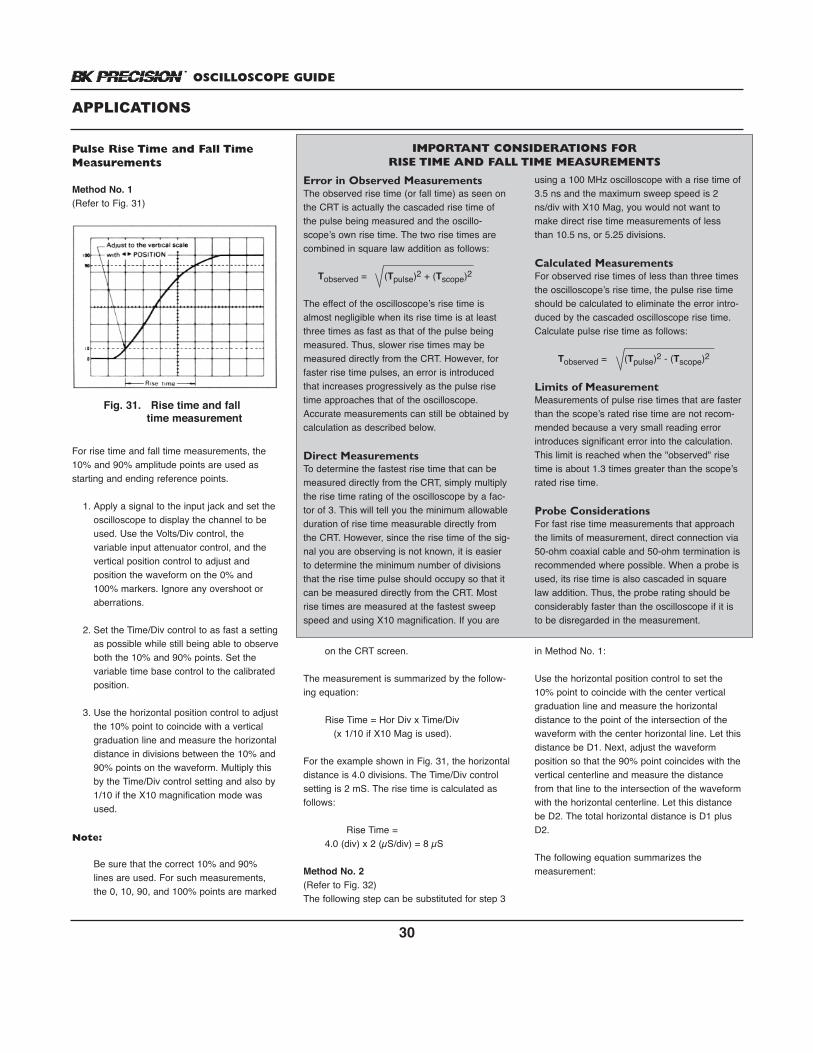
in Method No. 1:

Use the horizontal position control to set the10% point to coincide with the center verticalgraduation line and measure the horizontal distance to the point of the intersection of thewaveform with the center horizontal line. Let thisdistance be D1. Next, adjust the waveform position so that the 90% point coincides with thevertical centerline and measure the distancefrom that line to the intersection of the waveformwith the horizontal centerline. Let this distancebe D2. The total horizontal distance is D1 plusD2.

The following equation summarizes the measurement:

OSCILLOSCOPE GUIDE

30

Pulse Rise Time and Fall TimeMeasurements

Method No. 1(Refer to Fig. 31)

For rise time and fall time measurements, the10% and 90% amplitude points are used asstarting and ending reference points.

1. Apply a signal to the input jack and set the oscilloscope to display the channel to be used. Use the Volts/Div control, the variable input attenuator control, and the vertical position control to adjust and position the waveform on the 0% and 100% markers. Ignore any overshoot or aberrations.

2. Set the Time/Div control to as fast a settingas possible while still being able to observeboth the 10% and 90% points. Set the variable time base control to the calibrated position.

3. Use the horizontal position control to adjustthe 10% point to coincide with a vertical graduation line and measure the horizontal distance in divisions between the 10% and 90% points on the waveform. Multiply this by the Time/Div control setting and also by 1/10 if the X10 magnification mode was used.

Note:

Be sure that the correct 10% and 90% lines are used. For such measurements, the 0, 10, 90, and 100% points are marked

on the CRT screen.


Rise Time = Hor Div x Time/Div (x 1/10 if X10 Mag is used).

For the example shown in Fig. 31, the horizontaldistance is 4.0 divisions. The Time/Div controlsetting is 2 mS. The rise time is calculated asfollows:

Rise Time = 4.0 (div) x 2 (µS/div) = 8 µS

Method No. 2(Refer to Fig. 32)The following step can be substituted for step 3

APPLICATIONS

Fig. 31. Rise time and falltime measurement

Error in Observed MeasurementsThe observed rise time (or fall time) as seen onthe CRT is actually the cascaded rise time ofthe pulse being measured and the oscillo-scope’s own rise time. The two rise times arecombined in square law addition as follows:

Tobserved = (Tpulse)2 + (Tscope)2

The effect of the oscilloscope’s rise time isalmost negligible when its rise time is at leastthree times as fast as that of the pulse beingmeasured. Thus, slower rise times may bemeasured directly from the CRT. However, forfaster rise time pulses, an error is introducedthat increases progressively as the pulse risetime approaches that of the oscilloscope.Accurate measurements can still be obtained bycalculation as described below.

Direct MeasurementsTo determine the fastest rise time that can bemeasured directly from the CRT, simply multiplythe rise time rating of the oscilloscope by a fac-tor of 3. This will tell you the minimum allowableduration of rise time measurable directly fromthe CRT. However, since the rise time of the sig-nal you are observing is not known, it is easierto determine the minimum number of divisionsthat the rise time pulse should occupy so that itcan be measured directly from the CRT. Mostrise times are measured at the fastest sweepspeed and using X10 magnification. If you are

IMPORTANT CONSIDERATIONS FOR RISE TIME AND FALL TIME MEASUREMENTS

using a 100 MHz oscilloscope with a rise time of3.5 ns and the maximum sweep speed is 2ns/div with X10 Mag, you would not want tomake direct rise time measurements of lessthan 10.5 ns, or 5.25 divisions.

Calculated MeasurementsFor observed rise times of less than three timesthe oscilloscope’s rise time, the pulse rise timeshould be calculated to eliminate the error intro-duced by the cascaded oscilloscope rise time.Calculate pulse rise time as follows:

Tobserved = (Tpulse)2 - (Tscope)2

Limits of MeasurementMeasurements of pulse rise times that are fasterthan the scope’s rated rise time are not recom-mended because a very small reading errorintroduces significant error into the calculation.This limit is reached when the "observed" risetime is about 1.3 times greater than the scope’srated rise time.

Probe ConsiderationsFor fast rise time measurements that approachthe limits of measurement, direct connection via50-ohm coaxial cable and 50-ohm termination isrecommended where possible. When a probe isused, its rise time is also cascaded in squarelaw addition. Thus, the probe rating should beconsiderably faster than the oscilloscope if it isto be disregarded in the measurement.

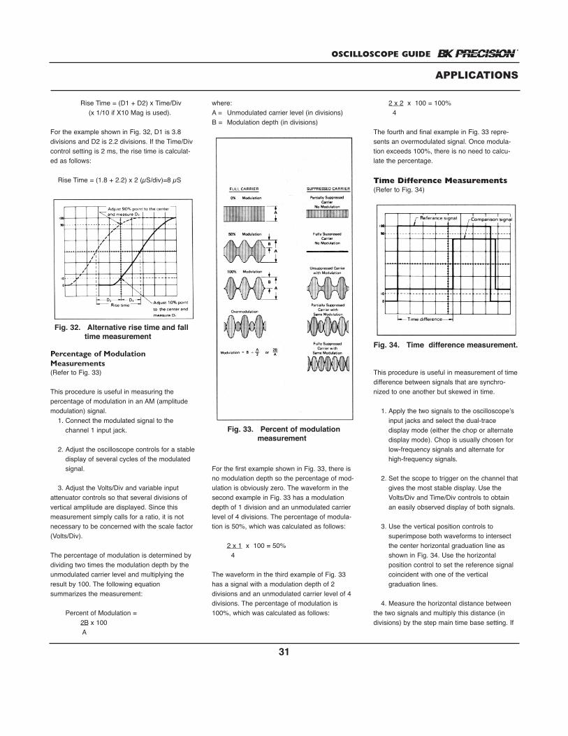
OSCILLOSCOPE GUIDE

31

Rise Time = (D1 + D2) x Time/Div (x 1/10 if X10 Mag is used).

For the example shown in Fig. 32, D1 is 3.8divisions and D2 is 2.2 divisions. If the Time/Divcontrol setting is 2 ms, the rise time is calculat-ed as follows:

Rise Time = (1.8 + 2.2) x 2 (µS/div)=8 µS

Percentage of ModulationMeasurements(Refer to Fig. 33)

This procedure is useful in measuring the percentage of modulation in an AM (amplitudemodulation) signal.

1. Connect the modulated signal to the channel 1 input jack.

2. Adjust the oscilloscope controls for a stabledisplay of several cycles of the modulated signal.

3. Adjust the Volts/Div and variable inputattenuator controls so that several divisions ofvertical amplitude are displayed. Since thismeasurement simply calls for a ratio, it is notnecessary to be concerned with the scale factor(Volts/Div).

The percentage of modulation is determined bydividing two times the modulation depth by theunmodulated carrier level and multiplying theresult by 100. The following equation summarizes the measurement:

Percent of Modulation =2B x 100A

where:A = Unmodulated carrier level (in divisions)B = Modulation depth (in divisions)

For the first example shown in Fig. 33, there isno modulation depth so the percentage of mod-ulation is obviously zero. The waveform in thesecond example in Fig. 33 has a modulationdepth of 1 division and an unmodulated carrierlevel of 4 divisions. The percentage of modula-tion is 50%, which was calculated as follows:

2 x 1 x 100 = 50%4

The waveform in the third example of Fig. 33has a signal with a modulation depth of 2 divisions and an unmodulated carrier level of 4divisions. The percentage of modulation is100%, which was calculated as follows:

2 x 2 x 100 = 100%4

The fourth and final example in Fig. 33 repre-sents an overmodulated signal. Once modula-tion exceeds 100%, there is no need to calcu-late the percentage.

Time Difference Measurements(Refer to Fig. 34)

This procedure is useful in measurement of timedifference between signals that are synchro-nized to one another but skewed in time.

1. Apply the two signals to the oscilloscope’s input jacks and select the dual-trace display mode (either the chop or alternate display mode). Chop is usually chosen for low-frequency signals and alternate for high-frequency signals.

2. Set the scope to trigger on the channel thatgives the most stable display. Use the Volts/Div and Time/Div controls to obtain an easily observed display of both signals.

3. Use the vertical position controls to superimpose both waveforms to intersect the center horizontal graduation line as shown in Fig. 34. Use the horizontal position control to set the reference signal coincident with one of the vertical graduation lines.

4. Measure the horizontal distance betweenthe two signals and multiply this distance (indivisions) by the step main time base setting. If

APPLICATIONS

Fig. 32. Alternative rise time and falltime measurement

Fig. 33. Percent of modulationmeasurement

Fig. 34. Time difference measurement.

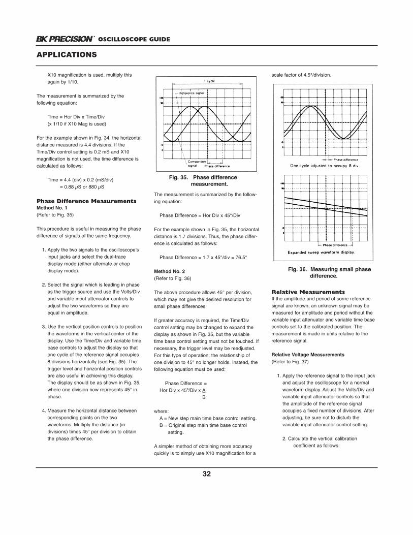
OSCILLOSCOPE GUIDE

32

X10 magnification is used, multiply this again by 1/10.


Time = Hor Div x Time/Div (x 1/10 if X10 Mag is used)

For the example shown in Fig. 34, the horizontaldistance measured is 4.4 divisions. If theTime/Div control setting is 0.2 mS and X10 magnification is not used, the time difference iscalculated as follows:

Time = 4.4 (div) x 0.2 (mS/div) = 0.88 µS or 880 µS

Phase Difference MeasurementsMethod No. 1(Refer to Fig. 35)

This procedure is useful in measuring the phasedifference of signals of the same frequency.

1. Apply the two signals to the oscilloscope’s input jacks and select the dual-trace display mode (either alternate or chop display mode).

2. Select the signal which is leading in phase as the trigger source and use the Volts/Div and variable input attenuator controls to adjust the two waveforms so they are equal in amplitude.

3. Use the vertical position controls to positionthe waveforms in the vertical center of the display. Use the Time/Div and variable timebase controls to adjust the display so that one cycle of the reference signal occupies 8 divisions horizontally (see Fig. 35). The trigger level and horizontal position controlsare also useful in achieving this display. The display should be as shown in Fig. 35,where one division now represents 45° in phase.

4. Measure the horizontal distance between corresponding points on the two waveforms. Multiply the distance (in divisions) times 45° per division to obtain the phase difference.


Phase Difference = Hor Div x 45°/Div

For the example shown in Fig. 35, the horizontaldistance is 1.7 divisions. Thus, the phase differ-ence is calculated as follows:

Phase Difference = 1.7 x 45°/div = 76.5°

Method No. 2(Refer to Fig. 36)

The above procedure allows 45° per division,which may not give the desired resolution forsmall phase differences.

If greater accuracy is required, the Time/Divcontrol setting may be changed to expand thedisplay as shown in Fig. 35, but the variabletime base control setting must not be touched. Ifnecessary, the trigger level may be readjusted.For this type of operation, the relationship ofone division to 45° no longer holds. Instead, thefollowing equation must be used:

Phase Difference =Hor Div x 45º/Div x A

B

where:A = New step main time base control setting.B = Original step main time base control

setting.

A simpler method of obtaining more accuracyquickly is to simply use X10 magnification for a

scale factor of 4.5°/division.

Relative MeasurementsIf the amplitude and period of some referencesignal are known, an unknown signal may bemeasured for amplitude and period without thevariable input attenuator and variable time basecontrols set to the calibrated position. Themeasurement is made in units relative to the reference signal.

Relative Voltage Measurements(Refer to Fig. 37)

1. Apply the reference signal to the input jack and adjust the oscilloscope for a normal waveform display. Adjust the Volts/Div and variable input attenuator controls so that the amplitude of the reference signal occupies a fixed number of divisions. After adjusting, be sure not to disturb the variable input attenuator control setting.

2. Calculate the vertical calibration coefficient as follows:

APPLICATIONS

Fig. 35. Phase differencemeasurement.

Fig. 36. Measuring small phasedifference.

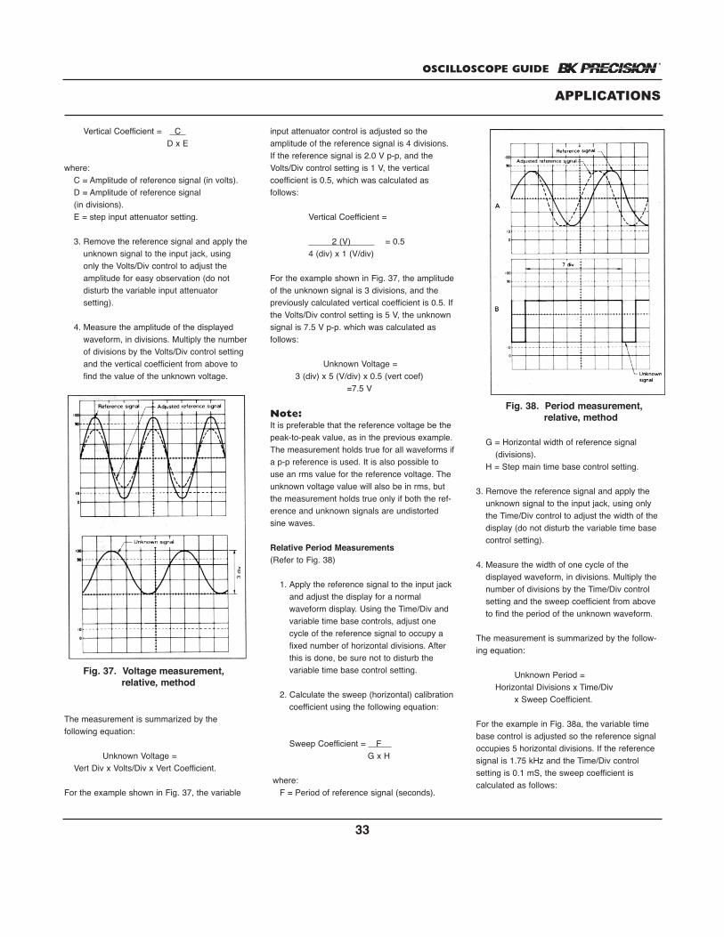
OSCILLOSCOPE GUIDE

33

Vertical Coefficient = C D x E

where:C = Amplitude of reference signal (in volts).D = Amplitude of reference signal (in divisions).E = step input attenuator setting.

3. Remove the reference signal and apply theunknown signal to the input jack, using only the Volts/Div control to adjust the amplitude for easy observation (do not disturb the variable input attenuator setting).

4. Measure the amplitude of the displayed waveform, in divisions. Multiply the numberof divisions by the Volts/Div control setting and the vertical coefficient from above to find the value of the unknown voltage.


Unknown Voltage = Vert Div x Volts/Div x Vert Coefficient.

For the example shown in Fig. 37, the variable

input attenuator control is adjusted so the amplitude of the reference signal is 4 divisions.If the reference signal is 2.0 V p-p, and theVolts/Div control setting is 1 V, the vertical coefficient is 0.5, which was calculated as follows:

Vertical Coefficient =

2 (V) = 0.54 (div) x 1 (V/div)

For the example shown in Fig. 37, the amplitudeof the unknown signal is 3 divisions, and thepreviously calculated vertical coefficient is 0.5. Ifthe Volts/Div control setting is 5 V, the unknownsignal is 7.5 V p-p. which was calculated as follows:

Unknown Voltage = 3 (div) x 5 (V/div) x 0.5 (vert coef)

=7.5 V

Note:It is preferable that the reference voltage be thepeak-to-peak value, as in the previous example.The measurement holds true for all waveforms ifa p-p reference is used. It is also possible touse an rms value for the reference voltage. Theunknown voltage value will also be in rms, butthe measurement holds true only if both the ref-erence and unknown signals are undistortedsine waves.

Relative Period Measurements(Refer to Fig. 38)

1. Apply the reference signal to the input jack and adjust the display for a normal waveform display. Using the Time/Div and variable time base controls, adjust one cycle of the reference signal to occupy a fixed number of horizontal divisions. After this is done, be sure not to disturb the variable time base control setting.

2. Calculate the sweep (horizontal) calibrationcoefficient using the following equation:

Sweep Coefficient = F G x H

where:F = Period of reference signal (seconds).

G = Horizontal width of reference signal (divisions).

H = Step main time base control setting.

3. Remove the reference signal and apply the unknown signal to the input jack, using only the Time/Div control to adjust the width of the display (do not disturb the variable time base control setting).

4. Measure the width of one cycle of the displayed waveform, in divisions. Multiply the number of divisions by the Time/Div control setting and the sweep coefficient from above to find the period of the unknown waveform.


Unknown Period = Horizontal Divisions x Time/Div

x Sweep Coefficient.

For the example in Fig. 38a, the variable timebase control is adjusted so the reference signaloccupies 5 horizontal divisions. If the referencesignal is 1.75 kHz and the Time/Div control setting is 0.1 mS, the sweep coefficient is calculated as follows:

APPLICATIONS

Fig. 37. Voltage measurement,relative, method

Fig. 38. Period measurement,relative, method

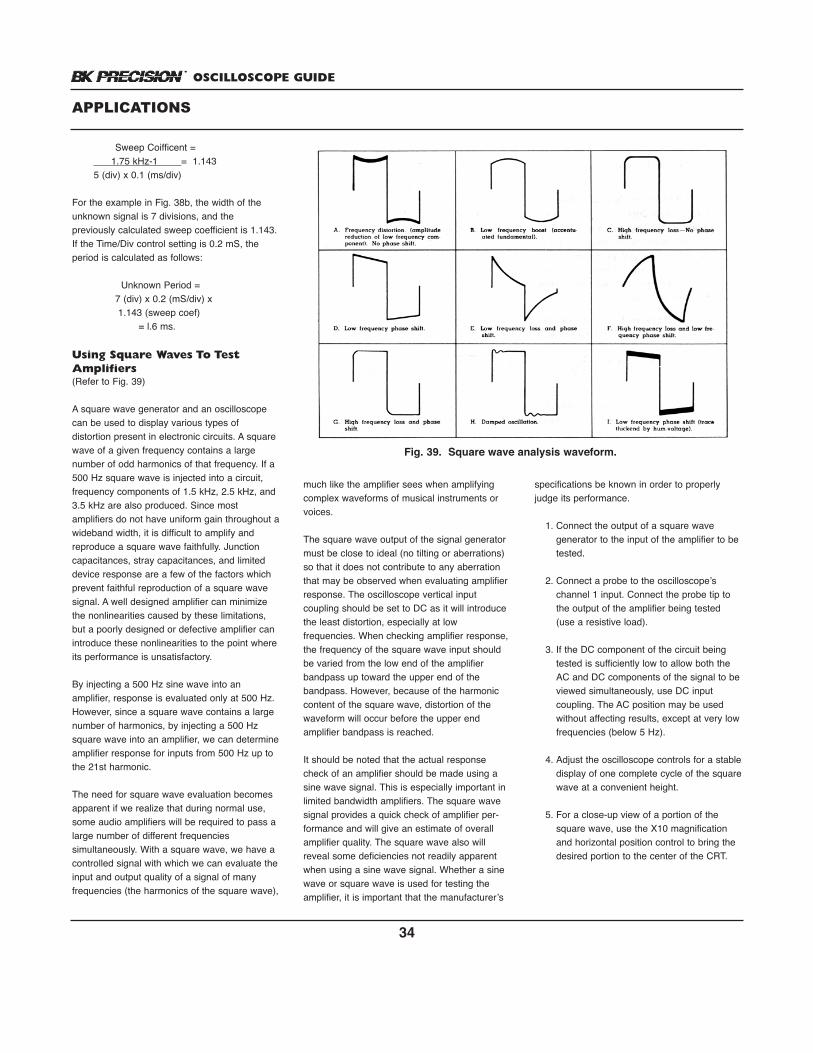
OSCILLOSCOPE GUIDE

34

Sweep Coifficent = 1.75 kHz-1 = 1.1435 (div) x 0.1 (ms/div)

For the example in Fig. 38b, the width of theunknown signal is 7 divisions, and the previously calculated sweep coefficient is 1.143.If the Time/Div control setting is 0.2 mS, theperiod is calculated as follows:

Unknown Period = 7 (div) x 0.2 (mS/div) x1.143 (sweep coef)

= l.6 ms.

Using Square Waves To TestAmplifiers(Refer to Fig. 39)

A square wave generator and an oscilloscopecan be used to display various types of distortion present in electronic circuits. A squarewave of a given frequency contains a largenumber of odd harmonics of that frequency. If a500 Hz square wave is injected into a circuit,frequency components of 1.5 kHz, 2.5 kHz, and3.5 kHz are also produced. Since most amplifiers do not have uniform gain throughout awideband width, it is difficult to amplify andreproduce a square wave faithfully. Junctioncapacitances, stray capacitances, and limiteddevice response are a few of the factors whichprevent faithful reproduction of a square wavesignal. A well designed amplifier can minimizethe nonlinearities caused by these limitations,but a poorly designed or defective amplifier can introduce these nonlinearities to the point whereits performance is unsatisfactory.

By injecting a 500 Hz sine wave into an amplifier, response is evaluated only at 500 Hz.However, since a square wave contains a largenumber of harmonics, by injecting a 500 Hzsquare wave into an amplifier, we can determineamplifier response for inputs from 500 Hz up tothe 21st harmonic.

The need for square wave evaluation becomesapparent if we realize that during normal use,some audio amplifiers will be required to pass alarge number of different frequencies simultaneously. With a square wave, we have acontrolled signal with which we can evaluate theinput and output quality of a signal of many frequencies (the harmonics of the square wave),

much like the amplifier sees when amplifyingcomplex waveforms of musical instruments orvoices.

The square wave output of the signal generatormust be close to ideal (no tilting or aberrations)so that it does not contribute to any aberrationthat may be observed when evaluating amplifierresponse. The oscilloscope vertical input coupling should be set to DC as it will introducethe least distortion, especially at low frequencies. When checking amplifier response,the frequency of the square wave input shouldbe varied from the low end of the amplifier bandpass up toward the upper end of the bandpass. However, because of the harmoniccontent of the square wave, distortion of thewaveform will occur before the upper end amplifier bandpass is reached.

It should be noted that the actual responsecheck of an amplifier should be made using asine wave signal. This is especially important inlimited bandwidth amplifiers. The square wavesignal provides a quick check of amplifier per-formance and will give an estimate of overallamplifier quality. The square wave also willreveal some deficiencies not readily apparentwhen using a sine wave signal. Whether a sinewave or square wave is used for testing theamplifier, it is important that the manufacturer’s

specifications be known in order to properlyjudge its performance.

1. Connect the output of a square wave generator to the input of the amplifier to be tested.

2. Connect a probe to the oscilloscope’s channel 1 input. Connect the probe tip to the output of the amplifier being tested (use a resistive load).

3. If the DC component of the circuit being tested is sufficiently low to allow both the AC and DC components of the signal to beviewed simultaneously, use DC input coupling. The AC position may be used without affecting results, except at very lowfrequencies (below 5 Hz).

4. Adjust the oscilloscope controls for a stabledisplay of one complete cycle of the squarewave at a convenient height.

5. For a close-up view of a portion of the square wave, use the X10 magnification and horizontal position control to bring the desired portion to the center of the CRT.

APPLICATIONS

Fig. 39. Square wave analysis waveform.

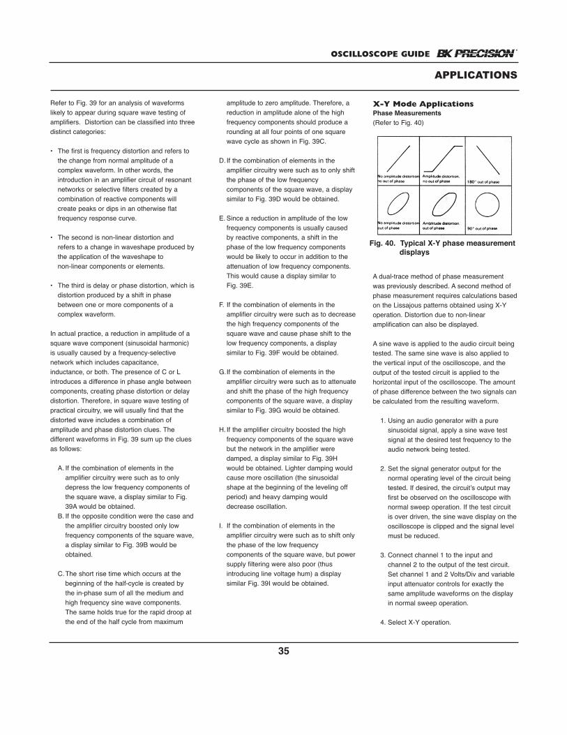
OSCILLOSCOPE GUIDE

35

Refer to Fig. 39 for an analysis of waveformslikely to appear during square wave testing ofamplifiers. Distortion can be classified into threedistinct categories:

• The first is frequency distortion and refers to the change from normal amplitude of a complex waveform. In other words, the introduction in an amplifier circuit of resonant networks or selective filters created by a combination of reactive components will create peaks or dips in an otherwise flat frequency response curve.

• The second is non-linear distortion and refers to a change in waveshape produced bythe application of the waveshape to non-linear components or elements.

• The third is delay or phase distortion, which is distortion produced by a shift in phase between one or more components of a complex waveform.

In actual practice, a reduction in amplitude of asquare wave component (sinusoidal harmonic)is usually caused by a frequency-selective network which includes capacitance, inductance, or both. The presence of C or Lintroduces a difference in phase angle betweencomponents, creating phase distortion or delaydistortion. Therefore, in square wave testing ofpractical circuitry, we will usually find that thedistorted wave includes a combination of amplitude and phase distortion clues. The different waveforms in Fig. 39 sum up the cluesas follows:

A. If the combination of elements in the amplifier circuitry were such as to only depress the low frequency components of the square wave, a display similar to Fig. 39A would be obtained.

B. If the opposite condition were the case andthe amplifier circuitry boosted only low frequency components of the square wave,a display similar to Fig. 39B would be obtained.

C.The short rise time which occurs at the beginning of the half-cycle is created by the in-phase sum of all the medium and high frequency sine wave components. The same holds true for the rapid droop at the end of the half cycle from maximum

amplitude to zero amplitude. Therefore, a reduction in amplitude alone of the high frequency components should produce a rounding at all four points of one square wave cycle as shown in Fig. 39C.

D. If the combination of elements in the amplifier circuitry were such as to only shift the phase of the low frequency components of the square wave, a display similar to Fig. 39D would be obtained.

E. Since a reduction in amplitude of the low frequency components is usually caused by reactive components, a shift in the phase of the low frequency components would be likely to occur in addition to the attenuation of low frequency components. This would cause a display similar to Fig. 39E.

F. If the combination of elements in the amplifier circuitry were such as to decreasethe high frequency components of the square wave and cause phase shift to the low frequency components, a display similar to Fig. 39F would be obtained.

G.If the combination of elements in the amplifier circuitry were such as to attenuateand shift the phase of the high frequency components of the square wave, a display similar to Fig. 39G would be obtained.

H. If the amplifier circuitry boosted the high frequency components of the square wave but the network in the amplifier were damped, a display similar to Fig. 39H would be obtained. Lighter damping would cause more oscillation (the sinusoidal shape at the beginning of the leveling off period) and heavy damping would decrease oscillation.

I. If the combination of elements in the amplifier circuitry were such as to shift only the phase of the low frequency components of the square wave, but power supply filtering were also poor (thus introducing line voltage hum) a display similar Fig. 39I would be obtained.

X-Y Mode ApplicationsPhase Measurements(Refer to Fig. 40)

A dual-trace method of phase measurementwas previously described. A second method ofphase measurement requires calculations basedon the Lissajous patterns obtained using X-Yoperation. Distortion due to non-linear amplification can also be displayed.

A sine wave is applied to the audio circuit beingtested. The same sine wave is also applied tothe vertical input of the oscilloscope, and theoutput of the tested circuit is applied to the horizontal input of the oscilloscope. The amountof phase difference between the two signals canbe calculated from the resulting waveform.

1. Using an audio generator with a pure sinusoidal signal, apply a sine wave test signal at the desired test frequency to the audio network being tested.

2. Set the signal generator output for the normal operating level of the circuit being tested. If desired, the circuit’s output may first be observed on the oscilloscope with normal sweep operation. If the test circuit is over driven, the sine wave display on theoscilloscope is clipped and the signal level must be reduced.

3. Connect channel 1 to the input and channel 2 to the output of the test circuit. Set channel 1 and 2 Volts/Div and variable input attenuator controls for exactly the same amplitude waveforms on the display in normal sweep operation.

4. Select X-Y operation.

APPLICATIONS

Fig. 40. Typical X-Y phase measurementdisplays

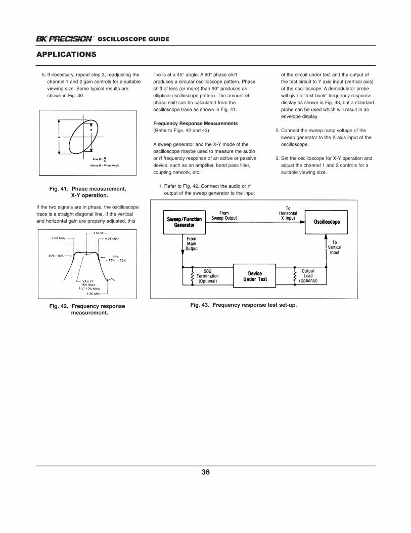
OSCILLOSCOPE GUIDE

36

5. If necessary, repeat step 3, readjusting the channel 1 and 2 gain controls for a suitableviewing size. Some typical results are shown in Fig. 40.

If the two signals are in phase, the oscilloscopetrace is a straight diagonal line. If the verticaland horizontal gain are properly adjusted, this

line is at a 45° angle. A 90° phase shift produces a circular oscilloscope pattern. Phaseshift of less (or more) than 90° produces anelliptical oscilloscope pattern. The amount ofphase shift can be calculated from the oscilloscope trace as shown in Fig. 41.

Frequency Response Measurements(Refer to Figs. 42 and 43)

A sweep generator and the X-Y mode of theoscilloscope maybe used to measure the audioor rf frequency response of an active or passivedevice, such as an amplifier, band pass filter,coupling network, etc.

1. Refer to Fig. 42. Connect the audio or rf output of the sweep generator to the input

of the circuit under test and the output of the test circuit to Y axis input (vertical axis) of the oscilloscope. A demodulator probe will give a "text book" frequency response display as shown in Fig. 43, but a standardprobe can be used which will result in an envelope display.

2. Connect the sweep ramp voltage of the sweep generator to the X axis input of the oscilloscope.

3. Set the oscilloscope for X-Y operation and adjust the channel 1 and 2 controls for a suitable viewing size.

APPLICATIONS

Fig. 43. Frequency response test set-up.

Fig. 41. Phase measurement,X-Y operation.

Fig. 42. Frequency responsemeasurement.

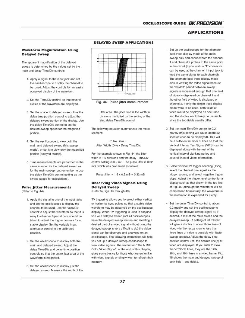
OSCILLOSCOPE GUIDE

37

Waveform Magnification UsingDelayed Sweep

The apparent magnification of the delayedsweep is determined by the values set by themain and delay Time/Div controls.

1. Apply a signal to the input jack and set the oscilloscope to display the channel to be used. Adjust the controls for an easily observed display of the waveform.

2. Set the Time/Div control so that several cycles of the waveform are displayed.

3. Set the scope to delayed sweep. Use the delay time position control to adjust the delayed sweep portion of the display. Usethe delay Time/Div control to set the desired sweep speed for the magnified portion.

4. Set the oscilloscope to view both the main and delayed sweep (Mix sweep mode), or set it to view only the magnifiedportion (delayed sweep).

5. Time measurements are performed in thesame manner for the delayed sweep as for the main sweep (but remember to usethe delay Time/Div control setting as the sweep speed for calculations).

Pulse Jitter Measurements(Refer to Fig. 44)

1. Apply the signal to one of the input jacks and set the oscilloscope to display the channel to be used. Use the Volts/Div control to adjust the waveform so that it iseasy to observe. Special care should be taken to adjust the trigger controls for a stable display. Set the variable input attenuator control to the calibrated position.

2. Set the oscilloscope to display both the main and delayed sweep. Adjust the delay Time/Div and delay time position controls so that the entire jitter area of thewaveform is magnified.

3. Set the oscilloscope to display just the delayed sweep. Measure the width of the

jitter area. The jitter time is the width in divisions multiplied by the setting of the step delay Time/Div control.

The following equation summarizes the meas-urement:

Pulse Jitter = Jitter Width (Div) x Delay Time/Div.

For the example shown in Fig. 44, the jitterwidth is 1.6 divisions and the delay Time/Divcontrol setting is 0.2 mS. The pulse jitter is 0.32mS, which was calculated as follows:

Pulse Jitter = 1.6 x 0.2 mS = 0.32 mS

Observing Video Signals UsingDelayed Sweep(Refer to Figs. 45 through 49)

TV triggering allows you to select either verticalor horizontal sync pulses so that a stable videowaveform may be observed on the oscilloscopedisplay. When TV triggering is used in conjunc-tion with delayed sweep (not all oscilloscopeshave the delayed sweep feature and isolating adesired part of a video signal without using thedelayed sweep is very difficult to do) the videosignal can be observed and analyzed on anoscilloscope. The following instructions will helpyou set up a delayed sweep oscilloscope toview video signals. The section on "The NTSCColor Video Signal", at the end of this chapter,gives some basics for those who are unfamiliarwith video signals or simply wish to refresh theirmemory.

1. Set up the oscilloscope for the alternate dual-trace display mode of the main sweep only and connect both the channel1 and channel 2 probes to the same pointin the circuit (if you wish, a "T" connector can be used at the channel 1 input jack tofeed the same signal to each channel). The alternate dual-trace display mode aids in viewing the video signal because the "holdoff" period between sweep signals is increased enough that one fieldof video is displayed on channel 1 and the other field of video is displayed on channel 2. If only the single trace display mode were to be used, both fields of video would be displayed on one trace and the display would likely be unusable since the two fields usually differ.

2. Set the main Time/Div control to 0.2 mS/div (this setting will cause about 32 lines of video to be displayed). This will be a sufficient number of lines so that the Vertical Interval Test Signal (VITS) can bedisplayed along with the rest of the vertical interval blanking period and several lines of video information.

3. Select vertical TV trigger coupling (TVV), select the channel one signal as the trigger source, and select negative triggerslope. Adjust the trigger level control for adisplay such as that shown in the top line of Fig. 45 (although the waveform will be compressed horizontally, the waveform in the illustration is expanded for clarity).

4. Set the delay Time/Div control to about 0.2 ms/div and set the oscilloscope to display the delayed sweep signal or, if desired, a mix of the main sweep and thedelayed sweep. (A setting of 20 mS/div will give a display of about three lines of video—further expansion to less than three lines of video is possible with faster sweep speeds.) Adjust the delay time position control until the desired line(s) of video are displayed. If you wish to view the VITS/VIR lines, they are the 17th, 18th, and 19th lines in a video frame. Fig.45 shows the main and delayed sweep ofboth field 1 and field 2.

APPLICATIONS

DELAYED SWEEP APPLICATIONS

Fig. 44. Pulse jitter measurement

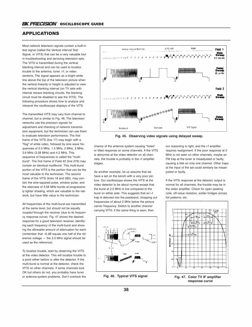
OSCILLOSCOPE GUIDE

38

Most network television signals contain a built-intest signal (called the Vertical Interval TestSignal, or VITS) that can be a very valuable toolin troubleshooting and servicing television sets.The VITS is transmitted during the verticalblanking interval and can be used to localizetrouble to the antenna, tuner, i-f, or video sections. The signal appears as a bright whiteline above the top of the television picture whenthe vertical linearity or height is adjusted to viewthe vertical blanking interval (on TV sets withinternal retrace blanking circuits, the blankingcircuit must be disabled to see the VITS). Thefollowing procedure shows how to analyze andinterpret the oscilloscope displays of the VITS.

The transmitted VITS may vary from channel tochannel, but is similar to Fig. 46. The televisionnetworks use the precision signals for adjustment and checking of network transmis-sion equipment, but the technician can use themto evaluate television performance. The firstframe of the VITS (line 17) may begin with a"flag" of white video, followed by sine wave fre-quencies of 0.5 MHz, 1.5 MHz, 2 MHz, 3 MHz,3.6 MHz (3.58 MHz) and 4.2 MHz. Thissequence of frequencies is called the "multi-burst". The first frame of Field #2 (line 279) maycontain an identical multiburst. This multi-burstportion of the VITS is the portion that can be themost valuable to the technician. The secondframe of the VITS (lines 18 and 280), may con-tain the sine-squared pulse, window pulse, andthe staircase of 3.58 MHz bursts at progressive-ly lighter shading, which are valuable to the net-work, but have little value to the technician.

All frequencies of the multi-burst are transmittedat the same level, but should not be equallycoupled through the receiver (due to its frequen-cy response curve). Fig. 47 shows the desiredresponse for a good television receiver, identify-ing each frequency of the multi-burst and show-ing the allowable amount of attenuation for each(remember that –6 dB equals one half of the ref-erence voltage — the 2.0 MHz signal should beused as the reference).

To localize trouble, start by observing the VITSat the video detector. This will localize trouble toa point either before or after the detector. If themulti-burst is normal at the detector, check theVITS on other channels. If some channels lookOK but others do not, you probably have tuneror antenna-system problems. Don’t overlook the

chance of the antenna system causing "holes"or tilted response on some channels. If the VITSis abnormal at the video detector on all chan-nels, the trouble is probably in the i-f amplifierstages.

As another example, let us assume that wehave a set on the bench with a very poor pic-ture. Our oscilloscope shows the VITS at thevideo detector to be about normal except thatthe burst at 2.0 MHz is low compared to theburst on either side. This suggests that an i-ftrap is detuned into the passband, chopping outfrequencies of about 2 MHz below the picturecarrier frequency. Switch to another channelcarrying VITS; if the same thing is seen, then

our reasoning is right, and the i-f amplifierrequires realignment. If the poor response at 2MHz is not seen on other channels, maybe anFM trap at the tuner is misadjusted or faulty,causing a bite on only one channel. Other trapsat the input of the set could similarly be misad-justed or faulty.

If the VITS response at the detector output isnormal for all channels, the trouble may be inthe video amplifier. Check for open peakingcoils, off-value resistors, solder bridges acrossfoil patterns, etc.

APPLICATIONS

Fig. 45. Observing video signals using delayed sweep.

Fig. 46. Typical VITS signal Fig. 47. Color TV IF amplifier response curve

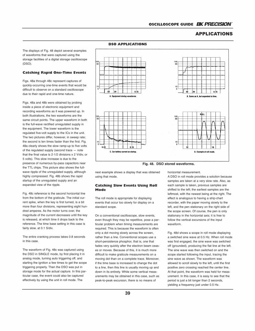
OSCILLOSCOPE GUIDE

39

The displays of Fig. 48 depict several examplesof waveforms that were captured using the storage facilities of a digital storage oscilloscope(DSO).

Catching Rapid One-Time Events

Figs. 48a through 48c represent captures ofquickly-occurring one-time events that would bedifficult to observe on a standard oscilloscopedue to their rapid and one-time nature.

Figs. 48a and 48b were obtained by probinginside a piece of electronic equipment andrecording waveforms as it was powered up. Inboth illustrations, the two waveforms are thesame circuit points. The upper waveform in bothis the full-wave rectified unregulated supply inthe equipment. The lower waveform is the regulated five-volt supply to the ICs in the unit.The two pictures differ, however, in sweep rate;the second is ten times faster than the first. Fig.48a clearly shows the slow ramp-up to five voltsof the regulated supply (second trace — notethat the final value is 2-1/2 divisions x 2 V/div, or5 volts). This slow increase is due to the presence of numerous by-pass capacitors nearthe TTL chips. This picture also shows the full-wave ripple of the unregulated supply, althoughhighly compressed. Fig. 48b shows the rapidstartup of the unregulated supply and anexpanded view of the ripple.

Fig. 48c reference is the second horizontal linefrom the bottom of the graticule. The initial cur-rent spike, when the key is first turned, is a bitmore than four divisions, representing eight hun-dred amperes. As the motor turns over, themagnitude of the current decreases until the keyis released, at which time it drops back to thereference. The time base setting in this case isfairly slow, at 0.1 S/div.

The entire cranking process takes 0.8 secondsin this case.

The waveform of Fig. 48c was captured usingthe DSO in SINGLE mode, by first placing it inanalog mode, turning auto triggering off, andstarting the ignition a few times to get the scopetriggering properly. Then the DSO was put instorage mode for the actual capture. In this par-ticular case, the event could also be capturedeffectively by using the unit in roll mode. The

next example shows a display that was obtainedusing that mode.

Catching Slow Events Using RollMode

The roll mode is appropriate for displayingevents that occur too slowly for display on astandard scope.

On a conventional oscilloscope, slow events,even though they may be repetitive, pose a par-ticular problem when timing measurements arerequired. This is because the waveform is oftenonly a dot moving slowly across the screen,rather than a line. Conventional scopes use ashort-persistence phosphor, that is, one thatfades very quickly after the electron beam ceas-es or moves. Because of this, it is much moredifficult to make graticule measurements on amoving dot than on a complete trace. Moreover,if the time base is increased to change the dotto a line, then this line is usually moving up anddown in its entirety. While some vertical meas-urements may be obtained in this case, such aspeak-to-peak excursion, there is no means of

horizontal measurement.A DSO in roll mode provides a solution becausesamples are taken at a very slow rate. Also, aseach sample is taken, previous samples areshifted to the left; the earliest samples are theleftmost, with the newest being at the right. Theeffect is analogous to having a strip-chartrecorder, with the paper moving slowly to theleft, and the pen stationary on the right side ofthe scope screen. Of course, the pen is onlystationary in the horizontal axis; it is free to follow the vertical excursions of the input waveform.

Fig. 48d shows a scope in roll mode displayinga switched sine wave at 0.5 Hz. When roll modewas first engaged, the sine wave was switchedoff (grounded), producing the flat line at the left.The sine wave was then switched on and thescope started following the input, tracing thesine wave as shown. The waveform wasallowed to scroll slowly to the left, until the firstpositive zero crossing reached the center line.At that point, the waveform was held for meas-urement. In this case, it is easy to see that theperiod is just a bit longer than 2 seconds, yielding a frequency just under 0.5 Hz.

APPLICATIONS

DSO APPLICATIONS

Fig. 48. DSO stored waveforms.

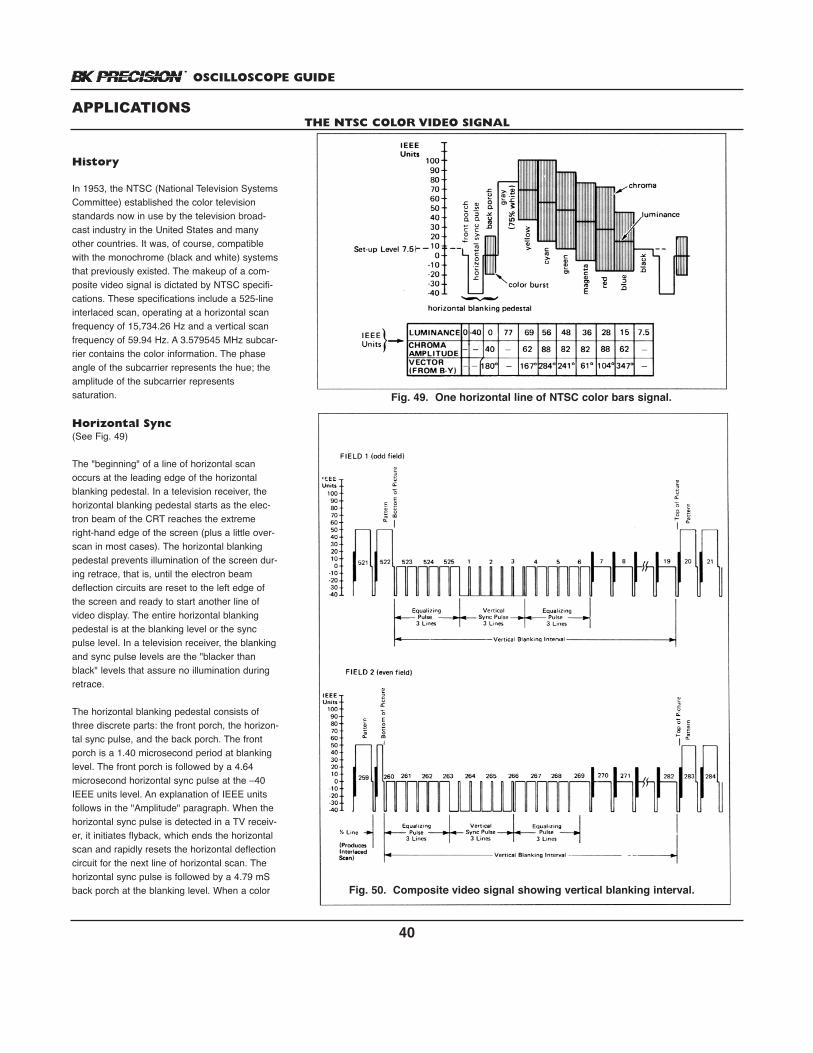
OSCILLOSCOPE GUIDE

40

History

In 1953, the NTSC (National Television SystemsCommittee) established the color televisionstandards now in use by the television broad-cast industry in the United States and manyother countries. It was, of course, compatiblewith the monochrome (black and white) systemsthat previously existed. The makeup of a com-posite video signal is dictated by NTSC specifi-cations. These specifications include a 525-lineinterlaced scan, operating at a horizontal scanfrequency of 15,734.26 Hz and a vertical scanfrequency of 59.94 Hz. A 3.579545 MHz subcar-rier contains the color information. The phaseangle of the subcarrier represents the hue; theamplitude of the subcarrier represents saturation.

Horizontal Sync(See Fig. 49)

The "beginning" of a line of horizontal scanoccurs at the leading edge of the horizontalblanking pedestal. In a television receiver, thehorizontal blanking pedestal starts as the elec-tron beam of the CRT reaches the extremeright-hand edge of the screen (plus a little over-scan in most cases). The horizontal blankingpedestal prevents illumination of the screen dur-ing retrace, that is, until the electron beamdeflection circuits are reset to the left edge ofthe screen and ready to start another line ofvideo display. The entire horizontal blankingpedestal is at the blanking level or the syncpulse level. In a television receiver, the blankingand sync pulse levels are the "blacker thanblack" levels that assure no illumination duringretrace.

The horizontal blanking pedestal consists ofthree discrete parts: the front porch, the horizon-tal sync pulse, and the back porch. The frontporch is a 1.40 microsecond period at blankinglevel. The front porch is followed by a 4.64microsecond horizontal sync pulse at the –40IEEE units level. An explanation of IEEE unitsfollows in the "Amplitude" paragraph. When thehorizontal sync pulse is detected in a TV receiv-er, it initiates flyback, which ends the horizontalscan and rapidly resets the horizontal deflectioncircuit for the next line of horizontal scan. Thehorizontal sync pulse is followed by a 4.79 mSback porch at the blanking level. When a color

APPLICATIONSTHE NTSC COLOR VIDEO SIGNAL

Fig. 49. One horizontal line of NTSC color bars signal.

Fig. 50. Composite video signal showing vertical blanking interval.

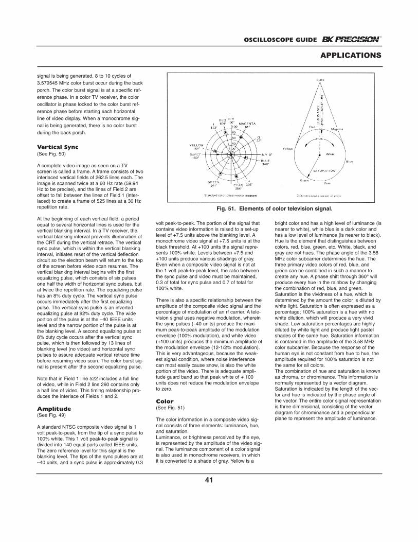
OSCILLOSCOPE GUIDE

41

signal is being generated, 8 to 10 cycles of3.579545 MHz color burst occur during the backporch. The color burst signal is at a specific ref-erence phase. In a color TV receiver, the coloroscillator is phase locked to the color burst ref-erence phase before starting each horizontalline of video display. When a monochrome sig-nal is being generated, there is no color burstduring the back porch.

Vertical Sync(See Fig. 50)

A complete video image as seen on a TVscreen is called a frame. A frame consists of twointerlaced vertical fields of 262.5 lines each. Theimage is scanned twice at a 60 Hz rate (59.94Hz to be precise), and the lines of Field 2 areoffset to fall between the lines of Field 1 (inter-laced) to create a frame of 525 lines at a 30 Hzrepetition rate.

At the beginning of each vertical field, a periodequal to several horizontal lines is used for thevertical blanking interval. In a TV receiver, thevertical blanking interval prevents illumination ofthe CRT during the vertical retrace. The verticalsync pulse, which is within the vertical blankinginterval, initiates reset of the vertical deflectioncircuit so the electron beam will return to the topof the screen before video scan resumes. Thevertical blanking interval begins with the firstequalizing pulse, which consists of six pulsesone half the width of horizontal sync pulses, butat twice the repetition rate. The equalizing pulsehas an 8% duty cycle. The vertical sync pulseoccurs immediately after the first equalizingpulse. The vertical sync pulse is an invertedequalizing pulse at 92% duty cycle. The wideportion of the pulse is at the –40 IEEE unitslevel and the narrow portion of the pulse is atthe blanking level. A second equalizing pulse at8% duty cycle occurs after the vertical syncpulse, which is then followed by 13 lines ofblanking level (no video) and horizontal syncpulses to assure adequate vertical retrace timebefore resuming video scan. The color burst sig-nal is present after the second equalizing pulse.

Note that in Field 1 line 522 includes a full lineof video, while in Field 2 line 260 contains onlya half line of video. This timing relationship pro-duces the interlace of Fields 1 and 2.

Amplitude(See Fig. 49)

A standard NTSC composite video signal is 1volt peak-to-peak, from the tip of a sync pulse to100% white. This 1 volt peak-to-peak signal isdivided into 140 equal parts called IEEE units.The zero reference level for this signal is theblanking level. The tips of the sync pulses are at–40 units, and a sync pulse is approximately 0.3

volt peak-to-peak. The portion of the signal thatcontains video information is raised to a set-uplevel of +7.5 units above the blanking level. Amonochrome video signal at +7.5 units is at theblack threshold. At +100 units the signal repre-sents 100% white. Levels between +7.5 and+100 units produce various shadings of gray.Even when a composite video signal is not atthe 1 volt peak-to-peak level, the ratio betweenthe sync pulse and video must be maintained,0.3 of total for sync pulse and 0.7 of total for100% white.

There is also a specific relationship between theamplitude of the composite video signal and thepercentage of modulation of an rf carrier. A tele-vision signal uses negative modulation, whereinthe sync pulses (–40 units) produce the maxi-mum peak-to-peak amplitude of the modulationenvelope (100% modulation), and white video(+100 units) produces the minimum amplitude ofthe modulation envelope (12-1/2% modulation).This is very advantageous, because the weak-est signal condition, where noise interferencecan most easily cause snow, is also the whiteportion of the video. There is adequate ampli-tude guard band so that peak white of + 100units does not reduce the modulation envelopeto zero.

Color(See Fig. 51)

The color information in a composite video sig-nal consists of three elements: luminance, hue,and saturation.Luminance, or brightness perceived by the eye,is represented by the amplitude of the video sig-nal. The luminance component of a color signalis also used in monochrome receivers, in whichit is converted to a shade of gray. Yellow is a

bright color and has a high level of luminance (isnearer to white), while blue is a dark color andhas a low level of luminance (is nearer to black).Hue is the element that distinguishes betweencolors, red, blue, green, etc. White, black, andgray are not hues. The phase angle of the 3.58MHz color subcarrier determines the hue. Thethree primary video colors of red, blue, andgreen can be combined in such a manner tocreate any hue. A phase shift through 360° willproduce every hue in the rainbow by changingthe combination of red, blue, and green.Saturation is the vividness of a hue, which isdetermined by the amount the color is diluted bywhite light. Saturation is often expressed as apercentage; 100% saturation is a hue with nowhite dilution, which will produce a very vividshade. Low saturation percentages are highlydiluted by white light and produce light pastelshades of the same hue. Saturation informationis contained in the amplitude of the 3.58 MHzcolor subcarrier. Because the response of thehuman eye is not constant from hue to hue, theamplitude required for 100% saturation is notthe same for all colors.The combination of hue and saturation is knownas chroma, or chrominance. This information isnormally represented by a vector diagram.Saturation is indicated by the length of the vec-tor and hue is indicated by the phase angle ofthe vector. The entire color signal representationis three dimensional, consisting of the vectordiagram for chrominance and a perpendicularplane to represent the amplitude of luminance.

APPLICATIONS

Fig. 51. Elements of color television signal.

oscilloscope applications guidebook - pedro … · alternate trigger — a dual-trace ... when the...

Documents