Mechanics of LaminatedMechanics of Laminated Composite Structuresp

Nachiketa TiwariNachiketa Tiwari

Indian Institute of Technology Kanpur

Lecture 22

Analysis of an Orthotropic Ply

Introduction

• Most of the composite materials are neither homogeneous nor isotropichomogeneous nor isotropic.– A homogeneousmaterial is one where properties are in the body, i.e. they do not depend on position in body.y, y p p y

– An isotropicmaterial is one where properties are direction independent. 

• Composites are inhomogeneous (or heterogeneous) as well as non‐isotropic materials.– In an inhomogeneous (or heterogeneous) material 

ti f t i l f i t t i tproperties of material vary from point‐to‐point.– A non‐isotropic material is one, where material properties depends on direction of observation. Thus, a material’sdepends on direction of observation. Thus, a material s modulus may be different in x, y, and z directions.

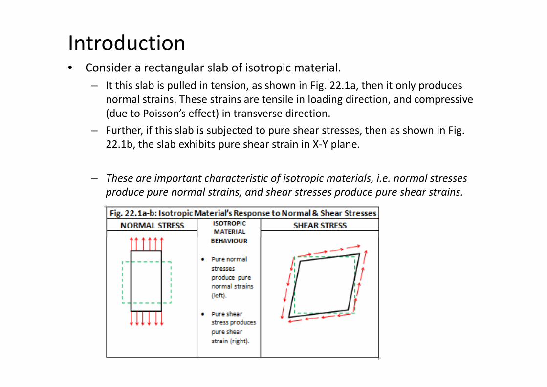
Introduction• Consider a rectangular slab of isotropic material. 

– It this slab is pulled in tension, as shown in Fig. 22.1a, then it only produces normal strains. These strains are tensile in loading direction, and compressive (due to Poisson’s effect) in transverse direction. 

– Further, if this slab is subjected to pure shear stresses, then as shown in Fig. 22.1b, the slab exhibits pure shear strain in X‐Y plane.p p

– These are important characteristic of isotropic materials, i.e. normal stresses produce pure normal strains and shear stresses produce pure shear strainsproduce pure normal strains, and shear stresses produce pure shear strains.

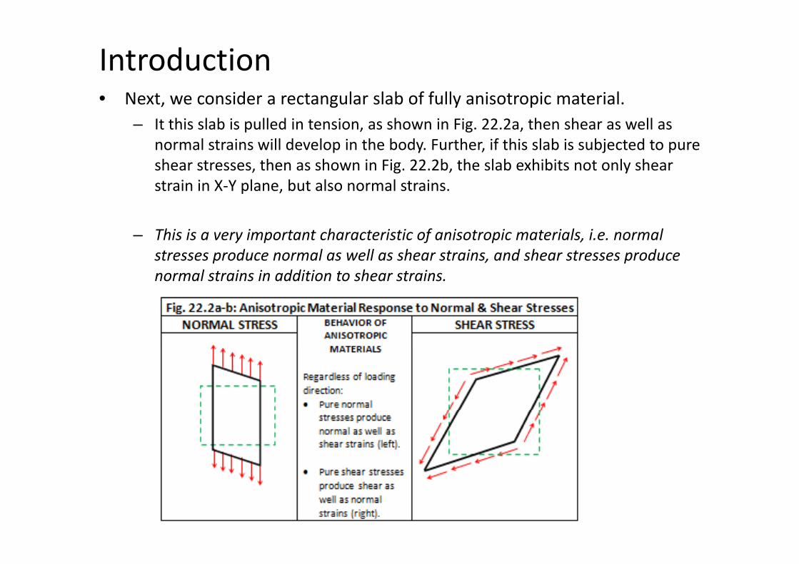
Introduction• Next, we consider a rectangular slab of fully anisotropic material. 

– It this slab is pulled in tension, as shown in Fig. 22.2a, then shear as well as normal strains will develop in the body. Further, if this slab is subjected to pure shear stresses, then as shown in Fig. 22.2b, the slab exhibits not only shear strain in X‐Y plane, but also normal strains.

– This is a very important characteristic of anisotropic materials, i.e. normal stresses produce normal as well as shear strains, and shear stresses produce normal strains in addition to shear strains.

Introduction• Finally, we consider a rectangular slab of orthotropic material. 

– In general this material behaves in ways very similar to anisotropic materialsIn general, this material behaves in ways very similar to anisotropic materials. Thus, when subjected to normal stresses, it will not only exhibit normal strains, but also shear strains.

– However, the response of these materials mimics that of isotropic material, if the edges of slab are parallel to a special set of three mutually perpendicular axesaxes. 

– The exact orientation of these three mutually perpendicular axes depends on h i l i l d i f idi i l ithe internal material structure, and in case of unidirectional composites, on the direction of fibers.

– These axes are known as natural material axes. Also, the planes for which these axes act as normals are known as planes of material symmetry. In case of unidirectional composites the direction of fiber is one such material axis, and is called longitudinal axis. The direction normal to the longitudinal axis is termed transverse axis.

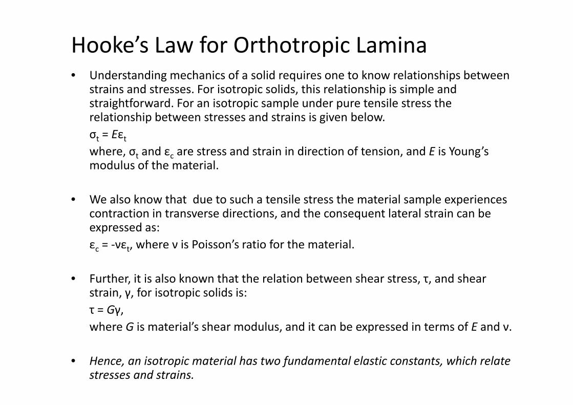
Hooke’s Law for Orthotropic Lamina• Understanding mechanics of a solid requires one to know relationships between 

strains and stresses. For isotropic solids, this relationship is simple and straightforward. For an isotropic sample under pure tensile stress the relationship between stresses and strains is given below.σt = Eεtwhere, σt and εc are stress and strain in direction of tension, and E is Young’s , t c , gmodulus of the material.

• We also know that due to such a tensile stress the material sample experiencesWe also know that  due to such a tensile stress the material sample experiences contraction in transverse directions, and the consequent lateral strain can be expressed as:εc = ‐νεt, where ν is Poisson’s ratio for the material. c t,

• Further, it is also known that the relation between shear stress, τ, and shear strain γ for isotropic solids is:strain, γ, for isotropic solids is: τ = Gγ, where G is material’s shear modulus, and it can be expressed in terms of E and ν. 

• Hence, an isotropic material has two fundamental elastic constants, which relate stresses and strains.

Hooke’s Law for Orthotropic Lamina

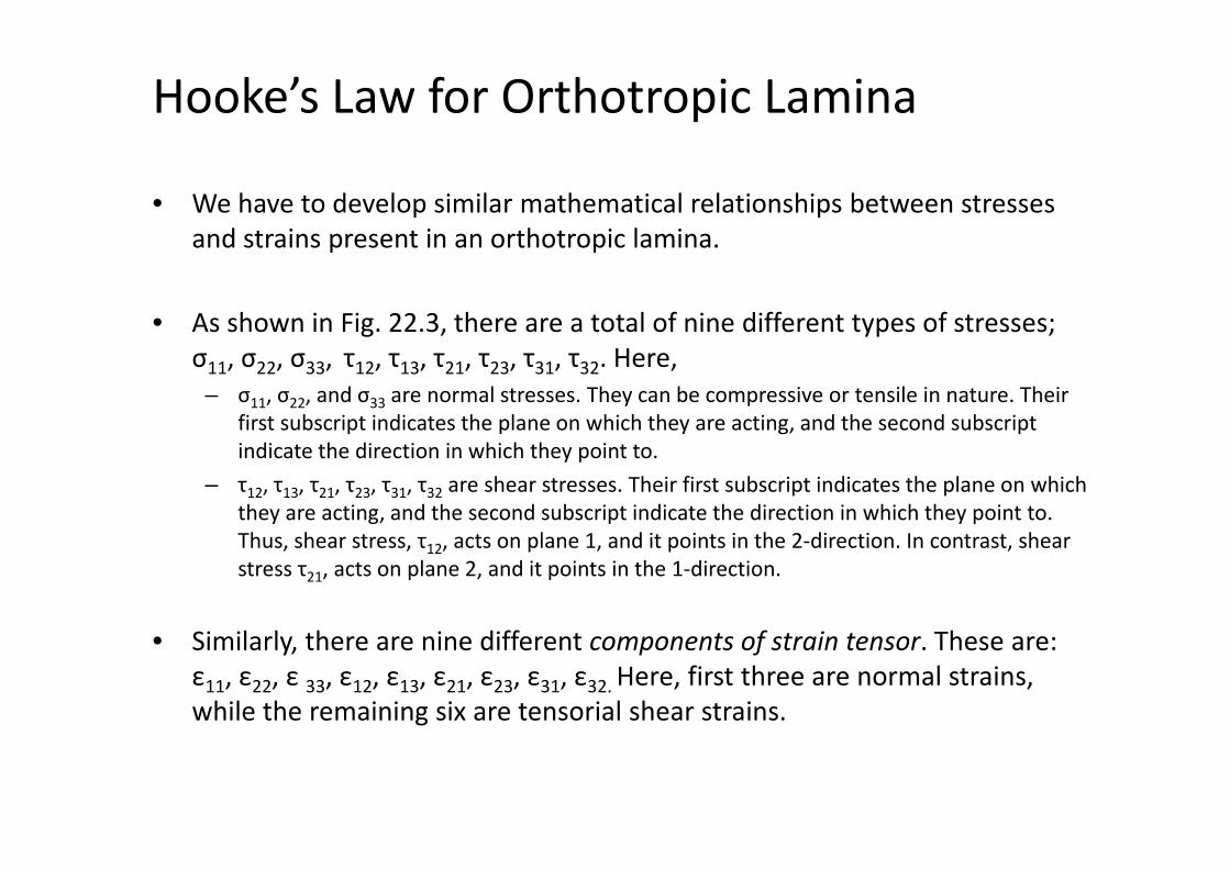
• We have to develop similar mathematical relationships between stresses and strains present in an orthotropic laminaand strains present in an orthotropic lamina.

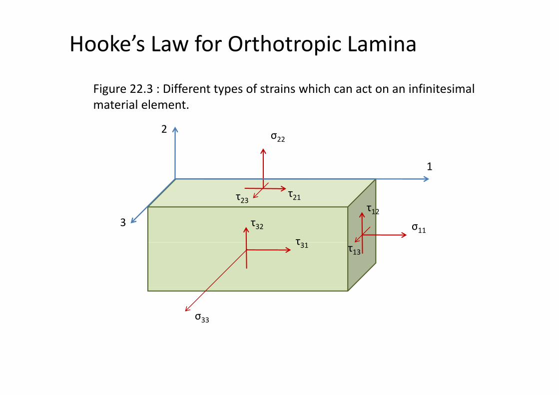
• As shown in Fig. 22.3, there are a total of nine different types of stresses; g ypσ11, σ22, σ33,  τ12, τ13, τ21, τ23, τ31, τ32. Here,

– σ11, σ22, and σ33 are normal stresses. They can be compressive or tensile in nature. Their first subscript indicates the plane on which they are acting, and the second subscript indicate the direction in which they point to.

– τ12, τ13, τ21, τ23, τ31, τ32 are shear stresses. Their first subscript indicates the plane on which they are acting, and the second subscript indicate the direction in which they point to. Th h l 1 d i i i h 2 di i I hThus, shear stress, τ12, acts on plane 1, and it points in the 2‐direction. In contrast, shear stress τ21, acts on plane 2, and it points in the 1‐direction. 

Si il l h i diff f i Th• Similarly, there are nine different components of strain tensor. These are: ε11, ε22, ε 33, ε12, ε13, ε21, ε23, ε31, ε32. Here, first three are normal strains, while the remaining six are tensorial shear strains.

Hooke’s Law for Orthotropic Lamina

Figure 22.3 : Different types of strains which can act on an infinitesimal material element.material element. 

σ222

τ21

1

τ

σ11

τ1221

3

τ23

τ

τ32

τ13τ31

σ33

Hooke’s Law for Orthotropic Lamina• The nine stress tensor components are related in a most general sense with 

nine strain components through the following equations.

• These are nine equations overall. Indices i, j, k, and l can assume values of 1, ese a e e equat o s o e a . d ces , j, , a d ca assu e a ues o ,2 or 3. Eijkl is the generalized stiffness tensor. The summation on left side is on indices k, and l. Thus, there are a total of 81 elastic constants for a fully anisotropic materialanisotropic material.

• Now, we can show from principal of equilibrium, that the values of cross shear stresses are equal. Thus, 

τ12 =  τ21 , τ23 =  τ32 , τ31 =  τ13. 

• This implies that values of Eijkl and Ejikl are same. This reduces the number of stiffness constants to 54. Further, we can also show through principles of geometry, the equality of cross‐shear strains. This further reduces the number of elastic constants to 36.

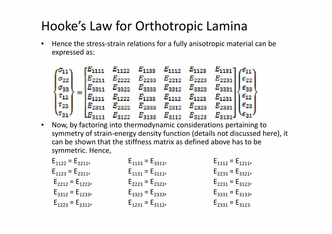
Hooke’s Law for Orthotropic Lamina• Hence the stress‐strain relations for a fully anisotropic material can be 

expressed as:

• Now, by factoring into thermodynamic considerations pertaining to symmetry of strain‐energy density function (details not discussed here), it can be shown that the stiffness matrix as defined above has to becan be shown that the stiffness matrix as defined above has to be symmetric. Hence,E1122 = E2211, E1133 = E3311, E1112 = E1211,E E E E E EE1123 = E2311, E1131 = E3111, E2233 = E3321,E2212 = E1222, E2223 = E2322, E2231 = E3122,E3312 = E1233, E3323 = E2333, E3331 = E3133,E1223 = E2312, E1231 = E3112, E2331 = E3123.

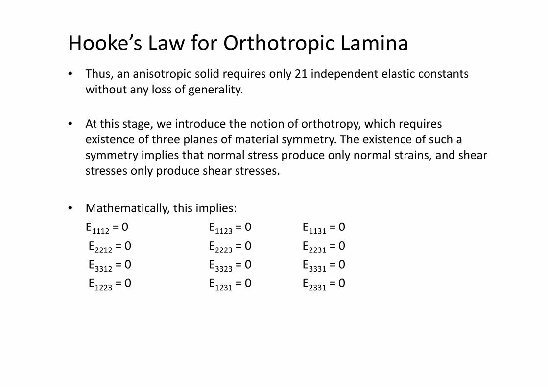
Hooke’s Law for Orthotropic Lamina• Thus, an anisotropic solid requires only 21 independent elastic constants 

without any loss of generality.

• At this stage, we introduce the notion of orthotropy, which requires existence of three planes of material symmetry. The existence of such a symmetry implies that normal stress produce only normal strains, and shear stresses only produce shear stresses.

• Mathematically, this implies:

E1112 = 0 E1123 = 0 E1131 = 0

E2212 = 0 E2223 = 0 E2231 = 0

E3312 = 0 E3323 = 0 E3331 = 0 

E 0 E 0 E 0E1223 = 0 E1231 = 0 E2331 = 0

Hooke’s Law for Orthotropic Lamina

• Thus, for an orthotropic material, the total number of elastic constants is 9. Using these constants, we can write the stress strain relation as:Using these constants, we can write the stress strain relation as:

σi = Qij∙εj i, j = 1, 2, 3, 4, 5, 6. (Eq. 22.1)

where,  

Qij is the stiffness matrix, σi represents six different stress components, and ε represents engineering strain vectorεj represents engineering strain vector. 

• Equation 22.1 is a generalized Hooke’s Law for orthotropic solids.

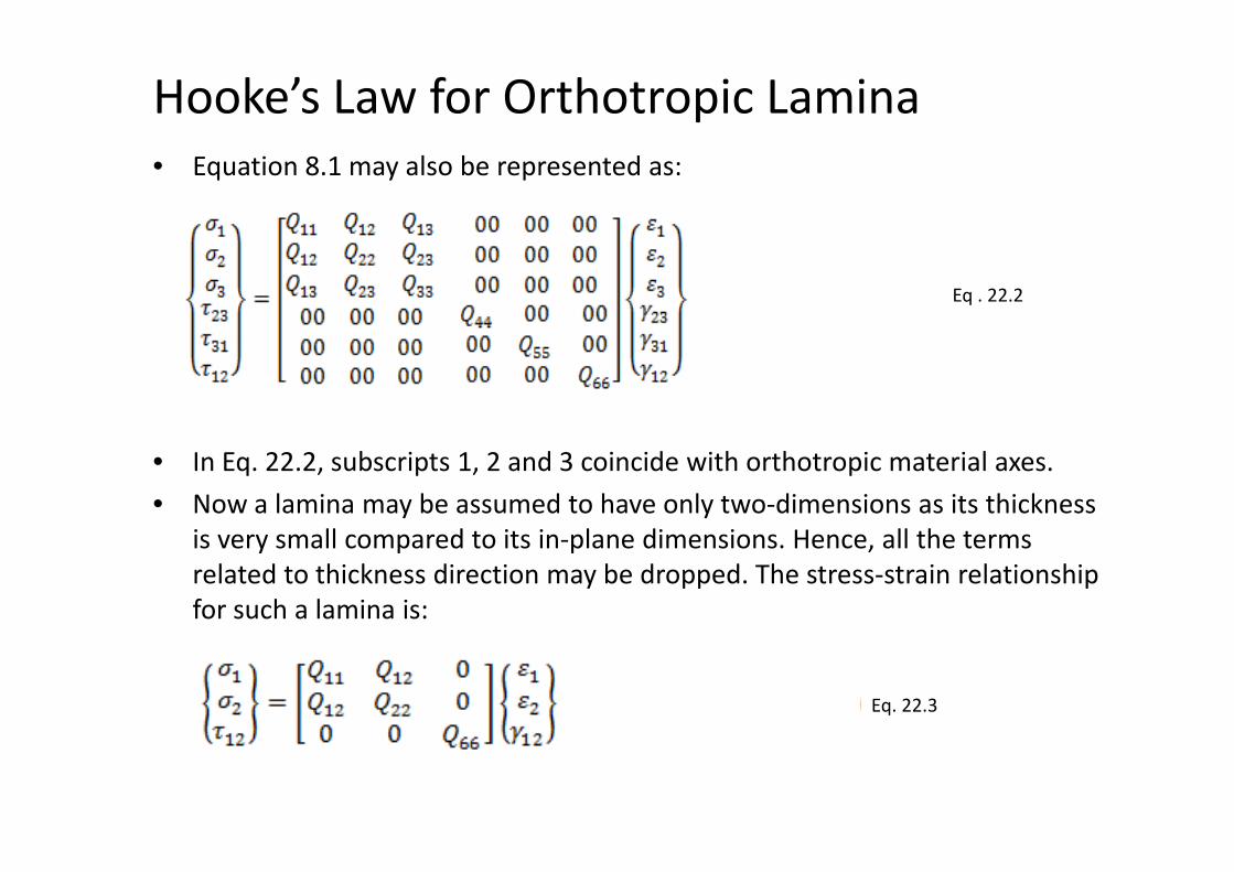
Hooke’s Law for Orthotropic Lamina• Equation 8.1 may also be represented as:

Eq . 22.2

• In Eq. 22.2, subscripts 1, 2 and 3 coincide with orthotropic material axes.

• Now a lamina may be assumed to have only two‐dimensions as its thickness is very small compared to its in plane dimensions Hence all the termsis very small compared to its in‐plane dimensions. Hence, all the terms related to thickness direction may be dropped. The stress‐strain relationship for such a lamina is:

Eq. 22.3

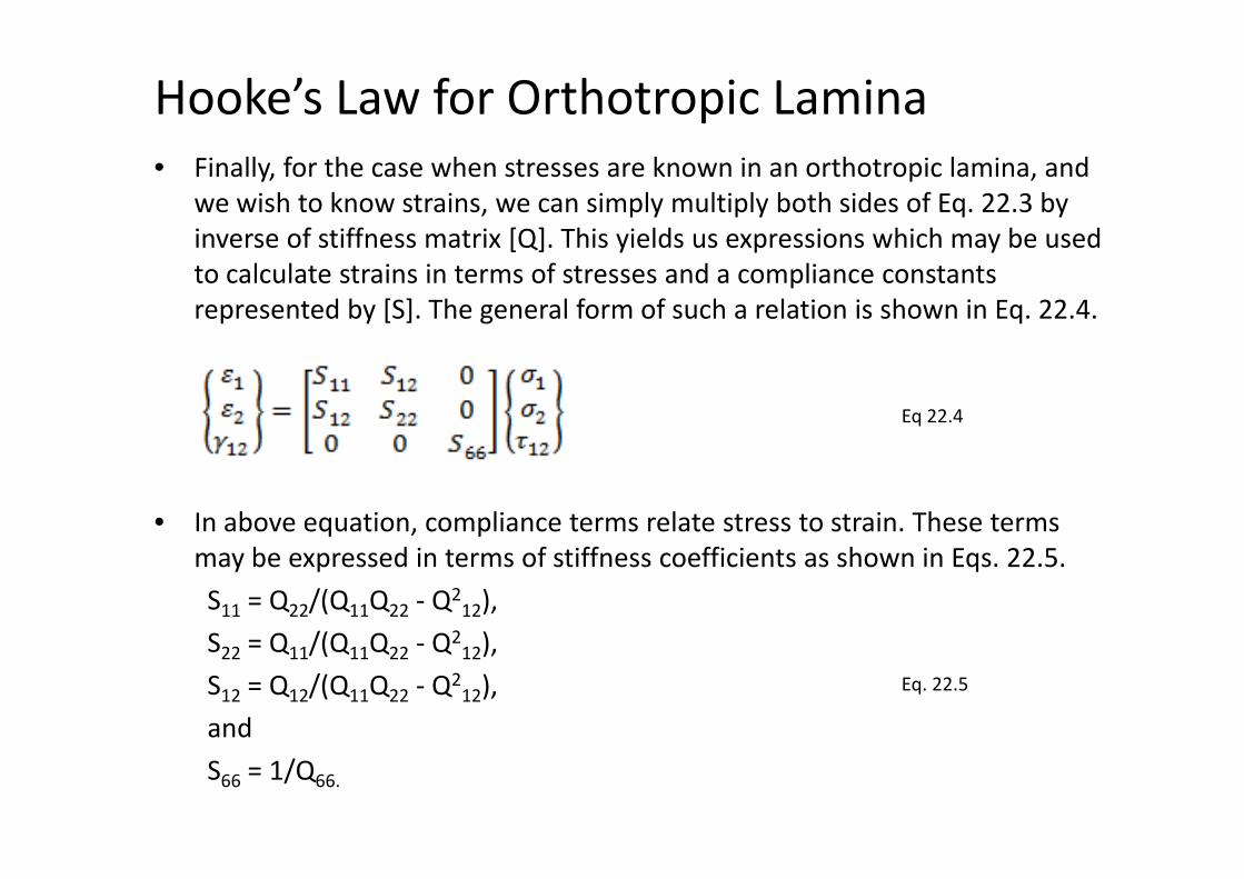
Hooke’s Law for Orthotropic Lamina• Finally, for the case when stresses are known in an orthotropic lamina, and 

we wish to know strains, we can simply multiply both sides of Eq. 22.3 by inverse of stiffness matrix [Q] This yields us expressions which may be usedinverse of stiffness matrix [Q]. This yields us expressions which may be used to calculate strains in terms of stresses and a compliance constants represented by [S]. The general form of such a relation is shown in Eq. 22.4.

Eq 22.4

• In above equation, compliance terms relate stress to strain. These terms may be expressed in terms of stiffness coefficients as shown in Eqs. 22.5. 

S11 = Q22/(Q11Q22 ‐ Q212), 

S Q /(Q Q Q2 )S22 = Q11/(Q11Q22 ‐ Q212),

S12 = Q12/(Q11Q22 ‐ Q212), (Eq. 8.5)

and

Eq. 22.5

S66 = 1/Q66.

Hooke’s Law for Orthotropic Lamina• Similarly, following equation may be used to find out stiffness constants of 

an orthotropic lamina, if its compliance coefficients were known. 

Q S /(S S S2 )Q11 = S22/(S11S22 ‐ S212), 

Q22 = S11/(S11S22 ‐ S212),

Q12 = S12/(S11S22 ‐ S212), (Eq. 8.6)Eq. 22.6Q12 S12/(S11S22 S 12), ( q. 8.6)

and

Q66 = 1/S66.

• It needs to be reiterated here that Eqs. 22.3 to 22.6 are only applicable for a two‐dimensional orthotropic lamina Such materials require only fourtwo dimensional orthotropic lamina. Such materials require only four independent elastic constants. For a three‐dimensional orthotropic lamina, nine elastic constants are needed. 

• Thus, understanding of three‐dimensional orthotropy involves more complexity compared to that of isotropy or two‐dimensional orthotropy.p y p py py